Sullivan 1

Borrowing During Unemployment: Unsecured Debt as a Safety Net

James X. Sullivan†

Abstract: This paper examines whether unsecured credit markets help disadvantaged households

supplement temporary shortfalls in earnings by investigating how unsecured debt responds to

unemployment-induced earnings losses. Results indicate that very low asset households—those

in the bottom decile of total assets—do not borrow in response to these shortfalls. However,

other low asset households do borrow, increasing unsecured debt by more than 11 cents per

dollar of earnings lost. In contrast, wealthy households do not increase unsecured debt during

unemployment. The evidence suggests that very low asset households do not have sufficient

access to unsecured credit to smooth consumption over transitory unemployment spells.

† James X. Sullivan is an Assistant Professor in the Department of Economics and Econometrics

at the University of Notre Dame. The author thanks Joseph Altonji, Bruce Meyer, Christopher

Taber, and two anonymous referees for their helpful comments and suggestions and Jonathan

Gruber for sharing his unemployment insurance benefit simulation model. The Joint Center for

Poverty Research (JCPR) provided generous support for this work. The author also benefited

from the comments of Gadi Barlevy, Kerwin Charles, Ulrich Doraszelski, Greg Duncan, Gary

Engelhardt, Charles Grant, Luojia Hu, Brett Nelson, Marianne Page, Henry Siu, Robert

Vigfusson, Thomas Wiseman, and seminar participants at the Board of Governors of the Federal

Reserve System, the Bureau of Labor Statistics, the European University Institute, the Federal

Reserve Bank of Chicago, the Federal Reserve Bank of St. Louis, the College of the Holy Cross,

the JCPR, Northwestern University, the University of Connecticut, the University of Notre

Dame, the University of Western Michigan, and the U.S. Census Bureau. The data used in this

Sullivan 2

article can be obtained beginning [date six months after publication] through [three years hence]

from James X. Sullivan, University of Notre Dame, 447 Flanner Hall, Notre Dame, IN, 46556,

sullivan.197@nd.edu.

Sullivan 3

I. Introduction

An extensive and growing literature examines how households smooth consumption in

response to idiosyncratic income shocks. Many of these studies focus on the role played by

government programs such as unemployment insurance (Gruber 1997; Browning and Crossley

2001), welfare (Gruber 2000), or food stamps (Blundell and Pistaferri 2003). Other studies have

considered how households insure via private transfers (Bentolila and Ichino Forthcoming), or

self-insure against income shocks through the earnings of other household members (Cullen and

Gruber 2000), by postponing purchases of durable goods (Browning and Crossley 2001), or by

refinancing mortgage debt (Hurst and Stafford 2004).

This paper contributes to this literature by considering another mechanism by which

families can maintain consumption during an income shortfall—borrowing through unsecured

credit markets.1 There are important reasons to focus on unsecured credit markets in this context.

First, unlike other components of net worth, unsecured debt is potentially available to families

that have no assets to liquidate or to collateralize loans. Thus, these credit markets provide low

asset households with a unique mechanism for transferring their own income intertemporally.

Second, with recent expansions in these markets, unsecured credit is potentially available to a

substantial fraction of U.S. households. More than three-quarters of all U.S. households have a

credit card, and outstanding balances on revolving credit exceed $750 billion (Federal Reserve

2005). Recent research suggests that unsecured debt has become easier to obtain: limits on credit

cards have become increasingly more generous; unsecured debt as a percentage of household

income has grown; and the risk-composition of credit card loan portfolios has deteriorated

(Evans and Schmalensee 1999; Lupton and Stafford 2000; Gross and Souleles 2002; Lyons

2003).2 Moreover, growth in credit card debt has been most striking among households below

Sullivan 4

the poverty line. From 1983 to 1995, the share of poor households with at least one credit card

more than doubled, from 17 percent to 36 percent, while average balances among poor

households grew by a factor of 3.8, as compared to a factor of 2.9 for all households.3

This expansion of unsecured credit could have particularly important implications for

these low income households. Bird, Hagstrom, and Wild (1999) shows that average credit card

debt for low income households fell during the economic expansion of the mid to late 1980s, but

that outstanding credit card balances grew during the recession of 1990-1991. Observing this

countercyclical trend in credit cards balances, the authors speculate that poor households may

use credit cards to smooth consumption, implying that these credit markets effectively serve as a

safety net. The possibility that credit markets help households smooth consumption has very

important policy implications—if families can self-insure against transitory earnings variation,

then this diminishes the need for public transfers. Nevertheless, little is known about the degree

to which households use unsecured credit markets in response to income shocks.

The first part of this paper investigates whether unsecured debt plays an instrumental role

in a household's ability to smooth consumption by examining how borrowing responds to

unanticipated, temporary unemployment-induced earnings variation, and how this response

varies with asset holdings. The results show that very low asset households—those in the bottom

decile of the asset distribution—do not borrow from unsecured credit markets in response to

these idiosyncratic shocks. Thus, these credit markets are not serving as an important safety net

for these households. This finding is robust to a variety of different tests of sensitivity. In

contrast, other low asset households—those in the second and third deciles of the asset

distribution—increase unsecured debt on average by 11.5 to 13.4 cents for each dollar of

earnings lost due to unemployment. Among this group with assets, borrowing is particularly

Sullivan 5

responsive to these shocks for less educated households. There is little evidence that wealthier

households borrow during unemployment.

The second part of this paper considers several possible explanations for why very low

asset households do not borrow. The evidence presented here indicates that these households are

not relying on alternative sources in lieu of credit markets. I show that these households are not

able to fully smooth consumption over these temporary income shocks. I also present evidence

that these households tend to have very low credit limits and their applications for credit are

frequently denied. While I cannot rule out other possible explanations, such as precautionary

motives, the evidence presented here points to the fact that, despite recent expansions in

unsecured credit markets, very low asset households do not have sufficient access to these

markets to help smooth consumption in response to a large idiosyncratic shock.

The following section discusses the empirical literature examining how households insure

against income shocks as well as studies examining the sensitivity of consumption to known

income variation. I present a description of the empirical methodology in Section III and

describe the data in Section IV. The results are presented in Section V. Section VI examines

why very low asset households do not borrow. Sensitivity analyses are discussed in Section VII,

and conclusions are presented in Section VIII.

II. Related Literature

Several studies that examine consumption behavior in response to unanticipated income

shocks have shown that while many households are not fully insured against these shortfalls,

there is significant evidence of some smoothing in response to these shocks (Dynarski and

Gruber 1997). How do households smooth? For some households, government programs are

clearly an important source of consumption insurance. A few studies have shown that in the case

Sullivan 6

of unemployment-induced earnings shocks, unemployment insurance (UI) plays an important

role (Gruber 1997), particularly for low asset households (Browning and Crossley 2001). Other

research has shown that cash welfare helps women transitioning into single motherhood smooth

consumption; consumption for this group increases by 28 cents for each additional dollar of

potential benefits (Gruber 2000). Among a low income population, the response of food

consumption to a permanent income shock is dampened by a third after accounting for food

stamps (Blundell and Pistaferri 2003). Empirical studies have also shown that the consumption

smoothing role of private transfers from friends and family is small in the U.S. (Bentolila and

Ichino Forthcoming), particularly relative to the role of government transfers (Dynarski and

Gruber 1997).

Households may also self-insure against idiosyncratic income shocks by changing the

work effort of other family members, postponing expenditures on durable goods, or dissaving.

Research suggests that additional income from other family members does not play a significant

role (Dynarski and Gruber 1997), although some of the added worker effect is crowded out by

UI (Cullen and Gruber 2000). There is evidence that some households smooth non-durable

consumption by delaying purchases on durables (Browning and Crossley 2004), and these

durables are more responsive to income shocks for less educated households (Dynarski and

Gruber 1997). Households can self-insure against lost earnings by maintaining a buffer stock of

liquid assets, but evidence suggests that household saving is often not sufficient to insure against

larger shortfalls such as an unemployment spell. The median 25-64 year old worker only has

enough financial assets to cover 3 weeks of pre-separation earnings. This falls far short of the

average unemployment spell, which lasts about 13 weeks (Engen and Gruber 2001; Gruber

2001).

Sullivan 7

Alternatively, households with access to credit markets may borrow from future income

to supplement current shortfalls. These markets allow households to transfer income

intertemporally and provide some insurance against idiosyncratic shocks through default. To

date, the empirical research in this area has focused on secured debt. Hurst and Stafford (2004)

present evidence that secured credit markets help households smooth consumption. They show

that homeowners borrow against the equity in their home in order to smooth consumption. This

is especially true for households without a significant stock of liquid assets. They conclude that

homeowners with low levels of liquid assets who experience an unemployment shock were 19

percent more likely to refinance their mortgage.

Beyond Hurst and Stafford (2004), which only looks at homeowners, little is known

about the role that household saving or borrowing plays in smoothing consumption in response

to idiosyncratic shocks.4 However, there is a related empirical literature that tests the permanent

income hypothesis by examining consumption, saving, and borrowing behavior in response to

known or predictable variation in income. Attanasio (1999), Browning and Lusardi (1996), and

Carroll (1997) provide surveys of this literature. A few of these studies look directly at saving

and its components. For example, Flavin (1991) considers how several components of net worth

respond to predictable changes in income. Flavin considers changes in liquid assets as well as

changes in total debt including mortgages, but she does not examine components of debt. Her

results, which concentrate on “truly wealthy” households, show that 30 percent of an anticipated

increase in income is saved in liquid assets, 6 percent in purchases of durables, and 20 percent in

reductions in total debt. Similarly, for a subsample of high income households, Alessie and

Lusardi (1997) report that between 10 and 20 percent of an expected income change goes

towards reducing debt. Neither of these papers report results for unsecured debt or for non-

Sullivan 8

wealthy households. A closely related literature explores possible explanations for the excess

sensitivity of consumption to predictable changes in income including heterogeneity in

preferences or liquidity constraints (Zeldes 1989). Evidence from this literature suggests that

access to credit markets does affect consumption behavior. For example, Jappelli, Pischke, and

Souleles (1998) shows that consumption growth is sensitive to known income for households

that report being turned down for a loan.

This study contributes to the empirical literature in several ways. This is the first study to

test empirically the extent to which households borrow from unsecured credit markets in

response to earnings shocks.5 While previous research within the literature examining excess

sensitivity has looked at household borrowing behavior, my study is unique in that I examine

how borrowing responds to large idiosyncratic shocks, rather than predictable variation. These

shocks are arguably more difficult to insure against. Unlike earlier studies, I focus on low asset

households rather than the wealthy, and I examine unsecured debt. Unsecured credit markets are

a unique source of consumption smoothing for low asset households because they do not have a

buffer of savings to supplement income shortfalls. These credit markets are also interesting to

examine given the significant growth in non-collateralized debt over the past two decades—

growth which has been strongest among disadvantaged households. Additionally, this paper

provides further evidence on the importance of borrowing constraints. While previous research

in this literature has focused on differences in consumption behavior across different types of

households, this paper directly examines differences in borrowing behavior across different types

of households facing strong incentives to borrow. Lastly, this study presents estimates for the

responsiveness of consumption and other components of net worth that support findings from

previous research.

Sullivan 9

III. Methodology

In the absence of borrowing constraints, the permanent income hypothesis suggests that a

household facing a transitory income shortfall will dissave in order to smooth consumption. For

households with low initial assets, this implies that borrowing will respond to transitory income

variation.6 Measured changes in labor income for the head of household i, ∆Yi, can be

decomposed into a transitory (∆Yiτ ) and a permanent (∆µi) component: ∆Yi =∆Yi

τ + ∆µi. Then, to

examine how household borrowing responds to changes in transitory income, one could estimate

the following:

where ∆Di = Dit - Dit-1, and Dit represents the level of unsecured debt for household i at the end of

year t, ∆Yiτ = Yit

τ - Yit−1τ represents the change in transitory income, ∆µi = µit - µit-1 represents

adjustments to permanent income, and Xi is a vector of observable demographics that are

indicative of permanent income and preferences. Using Equation 1 to estimate the

responsiveness of borrowing to exogenous earnings changes presents several problems. First, in

survey data we observe ∆Yi, not ∆Yiτ and ∆µi, and it is difficult to distinguish between transitory

and permanent changes in income. Second, the labor supply decision, and therefore income, is

endogenous to the household borrowing decision. For example, households that face an

expenditure shock, such as a major house repair, that results in an increase in debt may respond

by working more. Third, the change in labor income in national surveys is likely to be measured

with error.

Addressing these concerns, I exploit the panel nature of the data to identify transitory and

exogenous changes in income resulting from an unemployment spell of the head of household i

iiiii XYD ξαµααα τ ++∆+∆+=∆ 3210(1)

Sullivan 10

that occurs at some point during year t as a result of: a layoff, illness or injury to the worker,

being discharged or fired, employer bankruptcy, or the employer selling the business. This

excludes quits and other voluntary separations that are less likely to be exogenous to borrowing

or consumption decisions. I also restrict attention to spells that last at least one month, as these

longer spells are less likely to be voluntary and more likely to have a significant impact on total

household income.7 To focus on unanticipated spells, I restrict the sample to households whose

heads are employed at the beginning of year t and have no spells of unemployment in year t-1.

This excludes the chronically unemployed as well as those that experience seasonal layoffs. To

restrict attention to transitory variation, I limit my sample to households whose heads are

employed in year t+1 and do not experience an unemployment spell in that year. This restriction

excludes spells that are likely to have a more permanent effect on expected future lifetime

earnings.

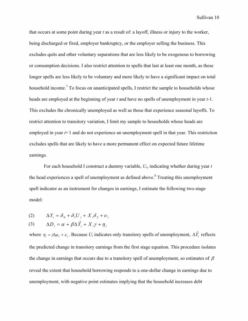
For each household I construct a dummy variable, Ui, indicating whether during year t

the head experiences a spell of unemployment as defined above.8 Treating this unemployment

spell indicator as an instrument for changes in earnings, I estimate the following two-stage

model:

where η γ µ εi i i= +∆ . Because Ui indicates only transitory spells of unemployment, iY∆ reflects

the predicted change in transitory earnings from the first stage equation. This procedure isolates

the change in earnings that occurs due to a transitory spell of unemployment, so estimates of β

reveal the extent that household borrowing responds to a one-dollar change in earnings due to

unemployment, with negative point estimates implying that the household increases debt

iiii

iiii

XYD

XUY

ηγβα

υδδδ

++∆+=∆

+++=∆ˆ

210(2)

(3)

Sullivan 11

holdings in response to a drop in earnings. Another approach would be to estimate directly the

effect of an unemployment spell on borrowing in a reduced form equation by regressing changes

in debt on the spell indicator. The main drawback of this approach is that by treating all spells

the same it ignores heterogeneity in the severity of spells across households. I verify that these

reduced form results are qualitatively consistent with the two-stage estimates.

The vector Xi includes a variety of characteristics of the household that influence saving

and borrowing decisions or that are indicative of permanent income, preferences, or consumption

needs. These include characteristics of the head in period t-1 such as educational attainment,

race, a cubic in age, and marital status, flexible controls for family size, changes in family size,

and an indicator for changes in marital status. The vector Xi also includes an indicator for

whether the level of unsecured debt at the end of year t-1 exceeds the annual earnings of the head

in that year to capture the fact that borrowing behavior may respond differently for households

that carry a substantial amount of unsecured debt initially. For example, these households may be

at or close to their borrowing limits, and therefore are more likely to be constrained than other

households. Data from the Survey of Consumer Finances (SCF) suggest that substantial existing

debt is an important reason for individuals being denied credit.

I also control for state-level characteristics that may affect the borrowing decision. The

current UI program, for example, provides supplemental income during unemployment spells,

and this transfer income is likely to affect the demand for liabilities to supplement earnings

shortfalls. To control for this, I include a measure of potential UI benefits in the vector Xi. I do

not include actual transfer income because take-up decisions are endogenous. I calculate

potential UI benefits as a function of state tax and benefit policies in year t-1, initial earnings,

total household income, marital status, and family size.9 The decision to borrow may also be

Sullivan 12

affected by the cost of bankruptcy, which varies across states. Accumulating debt and remaining

unemployed, for example, may be a more attractive option in states with generous bankruptcy

laws. Thus, I include in Xi an indicator for whether the state has a homestead exemption, the

value of this exemption, and the value of the personal property exemption in that year.10

This two-stage approach has several advantages. First, it isolates a transitory component

of labor income. Second, by capturing exogenous variation in earnings, this approach avoids the

biases that result from the endogeneity of labor supply. Third, this approach addresses concerns

with attenuation bias given the reasonable assumption that measurement error in this

unemployment indicator is uncorrelated with measurement error in changes in earnings.

Furthermore, these spells often result in significant earnings losses, providing a strong incentive

for the household to borrow.

Are these unemployment spells an appropriate instrument? To be a valid instrument these

spells must be sufficiently correlated with the changes in the earnings of the head, and they must

be uncorrelated withη i . These unemployment spells, which by construction last at least one

month, do have a significant impact on the earnings of the head. The estimates of δ1 in the first-

stage equation are large and very significant.11 Also, the rich set of demographic variables

available in both datasets allow me, in part, to control for household characteristics and other

components of income that are likely to be correlated with both the unemployment spell and

borrowing behavior. The data also allow me to identify spells that are arguably transitory and

unanticipated and therefore less likely to be correlated withη i .12 Although these spells are likely

to have both a permanent and a temporary component, others have argued that spells that are not

followed by subsequent displacements do not result in long term losses (Stevens 1997).13

Nevertheless, an important concern is that Ui may be correlated with unobservable household

Sullivan 13

characteristics or future expectations about earnings that affect the borrowing decision. This is

particularly problematic if the effect of Ui on future expectations is systematically different for

the different groups of households that I examine.

In the empirical analyses that follow, I examine the response of unsecured debt to income

shortfalls for households at different points in the ex ante asset distribution.14 The response for

low asset households is interesting because these households are potentially the most relevant

group to consider for questions concerning whether unsecured credit markets serve as a safety

net. Households with sizable asset holdings have the option of depleting these assets rather than

borrowing during unemployment spells. Thus, any borrowing for these households may in part

substitute for other sources of consumption smoothing such as dissaving. Households without

significant asset holdings, however, have few alternatives for supplementing lost earnings. They

do not have assets that they can liquidate or borrow against in secured credit markets. Thus,

unsecured credit markets are the only mechanism by which they can transfer their own income

intertemporally.15 If borrowing behavior for these low asset households responds to temporary

spells of unemployment then this would provide evidence that unsecured credit markets provide

an important source of supplemental income during earnings shortfalls. I also examine the

borrowing response at other points in the asset distribution to determine whether unsecured

credit markets are important for supplementing lost earnings for other households. I will use

several different measures of asset holdings including total gross assets, total financial assets,

and asset-to-earnings ratios.16 I also present evidence on how the responsiveness of consumption

varies across the asset distribution in order to determine the degree to which these households are

able to maintain well-being during unemployment.

IV. Data and Descriptive Results

Sullivan 14

The empirical analysis uses two independent surveys to examine household borrowing

and consumption behavior: the Survey of Income and Program Participation (SIPP) and the

Panel Study of Income Dynamics (PSID). The 1996 and 2001 Panels of the SIPP are used to

examine borrowing behavior. The SIPP provides demographic and economic information on a

random sample of households interviewed every 4 months from April 1996 to March 2000 (1996

Panel) and from February 2001 to January 2004 (2001 Panel). Information on the stock of assets

and liabilities, including unsecured debt, is provided annually in both panels of the SIPP.

Unsecured debt includes credit card debt, unsecured loans from financial institutions,

outstanding bills including medical bills, loans from individuals, and educational loans. For the

analysis that follows, I restrict attention to households that are interviewed in each of the first

nine waves of the panel (thus providing two observations on assets and liabilities for each

household), and whose heads in the third wave work full time and have positive earnings in each

of the first three waves and do not experience an unemployment spell during these first three

waves. To avoid confounding the borrowing decision with that of retirement, this initial sample

only includes households whose heads are between the ages of 20 and 63.17 Given these

restrictions, the results that follow are representative of working age households with strong

attachment to the labor force. The resulting sample includes 11,283 households from the 1996

Panel and 8,958 from the 2001 Panel.

In the SIPP, the first observation for debt is at the 3rd interview, prior to the observed

unemployment spells which are taken from the 4th through 6th waves of the panel. The second

debt observation is from the 6th interview, one year after the initial reported level of debt. To

avoid spells that are likely to have a more permanent effect on expected future lifetime earnings,

I also condition on the head being employed after the 6th wave.

Sullivan 15

The PSID is a longitudinal survey that has followed a nationally representative random

sample of families and their extensions since 1968. Waves are available annually through 1997

and biennially thereafter. Unlike the SIPP, the PSID provides information on food and housing

consumption.18 These data are used to examine how consumption responds to unemployment

induced earnings variation. I do not use all of the recent waves of the PSID because in some

waves I cannot identify unemployment spells that are more likely to be exogenous; from 1994

through 1997 the PSID did not include information on the reason why the head left a job, so

quits are not observed. Thus, to construct a sample that most closely overlaps with the SIPP

sample, I use data from the 1993, 1999, 2001, and 2003 waves of the PSID. Wealth supplement

data are available in 1989, 1994, 1999, 2001, and 2003.19 I determine the initial wealth holdings

for each household using the wealth reported at the most recent wealth supplement prior to the

current wave. I impose the same sample restrictions as those for the SIPP sample. In addition, I

exclude observations reporting zero food consumption. These restrictions yield a sample of

11,518.

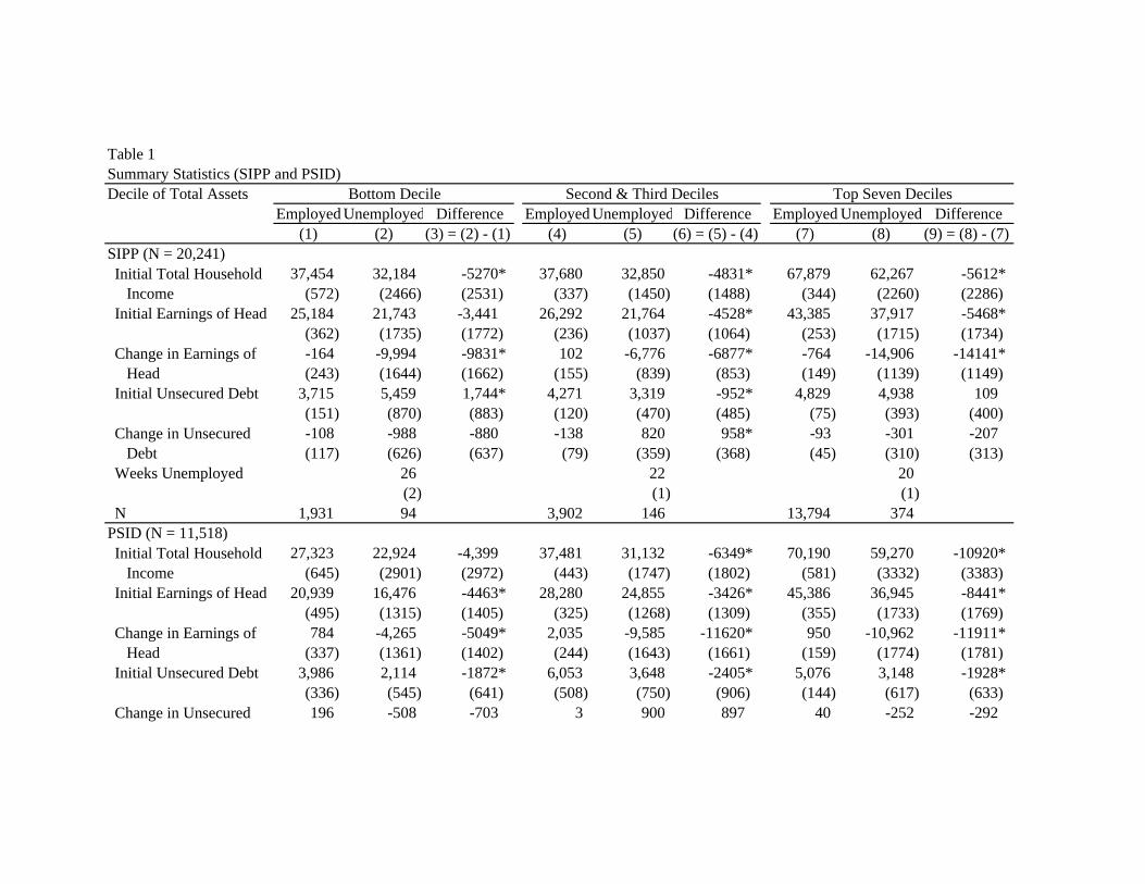
Descriptive statistics by asset holdings for the samples from the SIPP and the PSID are

presented in Table 1. As explained in the previous section, my identification strategy effectively

compares the borrowing behavior of those that do not experience an unemployment spell in a

given year (Columns 1, 4, and 7) to those that do become unemployed (Columns 2, 5, and 8).

The earnings shocks are not small—those that become unemployed experience a significant drop

in earnings both in absolute and relative terms. For households in the SIPP with very low

assets—those in the bottom decile of the distribution of total assets (Columns 1-3)—earnings fall

by nearly 50 percent. Comparing changes in debt across employment status for these low asset

households provides a preliminary look at how these households respond to exogenous

Sullivan 16

unemployment spells. Unsecured debt falls for the unemployed subsample in the SIPP both in

absolute terms (-988) and relative to those that do not experience an unemployment spell (-880),

although these changes are not statistically significant. Thus, there is little evidence from the

summary statistics that these very low asset households are borrowing to supplement lost

earnings during unemployment. On the other hand, there is some evidence that consumption falls

in response to the unemployment spell for this group. Those whose heads become unemployed

lower food and housing consumption by $1,531 more than households whose heads do not

experience an unemployment spell, and this difference is significant. Comparing these reductions

in relative consumption to the relative fall in earnings for the PSID sample suggests that

consumption falls by about 30 cents per dollar of lost earnings.

Table 1 also reports summary statistics for households at higher points in the asset

distribution. For example, those in the second and third deciles (Columns 4-6) are somewhat

more likely to borrow than those in the bottom decile. In the SIPP, the unemployed subsample

increases unsecured debt by $958 more than the employed subsample, and this difference is

statistically significant. This relative increase in borrowing for unemployed households may

suggest that households with assets are borrowing to supplement lost income. A relative drop in

earnings of $6,877 for this group implies that on average borrowing increases by about 14 cents

for each dollar of earnings lost. There is also evidence that food and housing consumption falls

for these unemployed households relative to those that do not lose their jobs, but this drop, as a

percentage of lost earnings, is less than half as large as the decrease for the very low asset group.

Relative changes in borrowing and consumption are much less noticeable for higher asset

households that become unemployed (Columns 7-9).

Sullivan 17

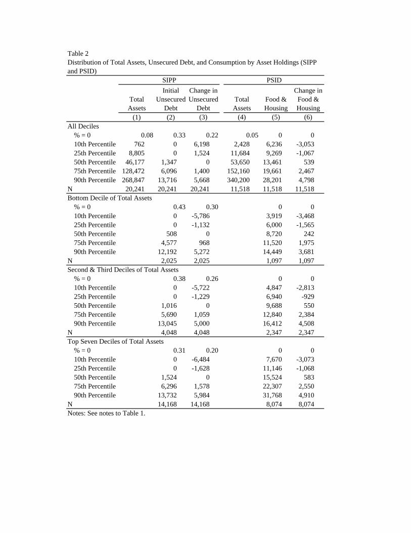
Table 2 shows the distributions of total assets, unsecured debt, and consumption for the

full samples, as well as for households at different points in the asset distribution. Eight percent

of all households have no assets. The distribution of unsecured debt is skewed. The median level

of initial debt for SIPP households is $1,347, but 33 percent of the households do not carry any

unsecured debt. A sizeable number of households also have no change in unsecured debt over

time—most of which carry zero debt in both periods. Potential complications with this non-

linearity are discussed in Section VII. Households at the bottom of the asset distribution are less

likely to borrow. 43 percent have no outstanding unsecured debt initially. Households at higher

points in the assets distribution hold more ex ante unsecured debt.20 They also spend more on

both food and housing, but the distributions of changes in consumption are fairly similar across

asset holdings.

As explained in Section III, the analyses focus on transitory changes in income that result

from temporary unemployment spells. To examine whether these unemployment spells have a

transitory effect on income, I exploit the panel nature of the SIPP to examine the long-term

impact of these spells on earnings and total household income. To this end, I regress these

outcomes on leads and lags of the unemployment spell in a model including demographic

controls and a household fixed effect:

itiitj

jitjit XUY υηγβ +++= ∑−=

+

3

2ln

where lnYit represents the log of earnings of the head (or total income) of household i in wave t,

Uit+j is an indicator of whether an unemployment spell occurs in wave t+j, Xit is a vector of the

same household demographics included in Equations 2 and 3, andη i is a household-specific

effect. Estimates of βj represent the effect of an unemployment spell in period t+j on an outcome

(4)

Sullivan 18

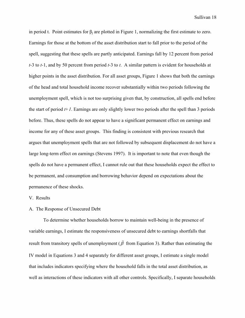
in period t. Point estimates for βj are plotted in Figure 1, normalizing the first estimate to zero.

Earnings for those at the bottom of the asset distribution start to fall prior to the period of the

spell, suggesting that these spells are partly anticipated. Earnings fall by 12 percent from period

t-3 to t-1, and by 50 percent from period t-3 to t. A similar pattern is evident for households at

higher points in the asset distribution. For all asset groups, Figure 1 shows that both the earnings

of the head and total household income recover substantially within two periods following the

unemployment spell, which is not too surprising given that, by construction, all spells end before

the start of period t+1. Earnings are only slightly lower two periods after the spell than 3 periods

before. Thus, these spells do not appear to have a significant permanent effect on earnings and

income for any of these asset groups. This finding is consistent with previous research that

argues that unemployment spells that are not followed by subsequent displacement do not have a

large long-term effect on earnings (Stevens 1997). It is important to note that even though the

spells do not have a permanent effect, I cannot rule out that these households expect the effect to

be permanent, and consumption and borrowing behavior depend on expectations about the

permanence of these shocks.

V. Results

A. The Response of Unsecured Debt

To determine whether households borrow to maintain well-being in the presence of

variable earnings, I estimate the responsiveness of unsecured debt to earnings shortfalls that

result from transitory spells of unemployment (β)

from Equation 3). Rather than estimating the

IV model in Equations 3 and 4 separately for different asset groups, I estimate a single model

that includes indicators specifying where the household falls in the total asset distribution, as

well as interactions of these indicators with all other controls. Specifically, I separate households

Sullivan 19

into four separate asset groups: those in the bottom decile (the baseline group), those in the

second and third deciles, those in the fourth and fifth deciles, and those in the top half of the

asset distribution.21 Alternative specifications examine households at different points in the

distribution of financial assets or asset-to-earnings ratios.

Table 3 reports IV estimates for the effect of unemployment-induced earnings variation

on borrowing (using SIPP data) and consumption (using PSID data). The results in Column 1

provide evidence on the responsiveness of unsecured debt for households at different points in

the distribution of total assets. The response of unsecured debt for households in the bottom

decile, β1, is positive, suggesting that unsecured borrowing decreases with unemployment-

induced earnings losses, although the point estimate is small and insignificant.22 This estimate

provides virtually no evidence that these very low asset households—those with less than $762

in total assets (Table 2)—borrow during unemployment spells. In fact, I reject a one-sided test

that borrowing increases by more than 3.2 cents for each dollar lost. The estimates of β1 for those

at the bottom of the distribution of financial assets (Column 4) or asset-to-earnings ratios

(Column 7) provide very similar evidence. These credit markets do not appear to be a safety net

for those at the very bottom of the asset distribution.23

For other low asset households—those in the second and third deciles of total assets

(Column 1)—unsecured debt responds significantly to a job loss, increasing by 13.4 cents

(β1+β2) for each dollar of earnings lost due to unemployment (p-value = 0.033). The results are

very similar for households in these same deciles of the distribution of financial assets (11.5

cents) or asset-to-earnings ratios (13.0 cents). The magnitude of this response is comparable to

other common sources for supplementing earnings losses. For example, Dynarski and Gruber

(1997) estimate that unemployment insurance supplements 7 to 22 cents of each dollar of lost

Sullivan 20

earnings due to unemployment. They estimate additional earnings of the spouse (the added

worker effect) to respond by 2 to 12 cents for each dollar lost.

In each case, the borrowing behavior for those in the second and third deciles is

significantly different from that of the lowest asset group (β2). Moreover, in nearly all cases, I

can reject the hypothesis that the borrowing behavior for this group is the same as any of the

other asset groups. For example, the estimates indicate that these households borrow 15.4 cents

(β4-β2) more per dollar lost than those in the top half of the total asset distribution (p-value =

0.020). There is little evidence that higher asset households borrow in response to an

unemployment-induced earnings loss.

B. Consumption and Components of Net Worth

The fact that borrowing does not change in response to unemployment spells for some

households indicates that these households are either supplementing income via other sources or

reducing consumption. Table 3 also presents estimates of the responsiveness of consumption to

unemployment-induced earnings for two measures of consumption that are observable in the

PSID—food and food plus housing.24 The point estimates for those in the bottom decile suggest

that food consumption falls by between 8 and 9 cents for each dollar of lost earnings, but these

estimates are not statistically significant. For the combined measure of food plus housing

consumption, the IV estimates show a larger response.25 For those in the bottom decile of

financial assets (Column 6), food plus housing consumption falls by 31.3 cents for each dollar of

earnings lost, and this estimates is significant.

For households with higher assets there is evidence that the consumption response is

smaller—β2, β3, and β4 are all negative—and some of these differences are significant (Column

6). There is some evidence that food and housing consumption falls during unemployment for

Sullivan 21

those in the second and third deciles, but the magnitude of this response is just over a third of

that for those in the bottom decile of total assets. In all cases the response of both food and food

plus housing consumption is small (less than 3.3 cents per dollar lost) and insignificant for

households in the top half of the asset distribution (β1+β4). Similar results are evident for those

in the fourth or fifth deciles, except when grouped by financial assets (Columns 5 and 6).

These results for consumption are consistent with a number of previous studies that have

examined the responsiveness of consumption to unemployment. For example, Dynarski and

Gruber (1997) also find that unemployment spells result in a reduction in consumption for some

households, although they do not focus on very low asset households. For a sample of

households in the bottom 75 percent of the financial assets distribution, they find that food and

housing consumption falls by 25.5 cents for each dollar of earnings lost. Browning and Crossley

(2001) also report drops in expenditures during unemployment for a low asset sample. Stephens

(2001) shows that job displacements result in persistent drops in consumption.

As additional evidence on how households supplement unemployment-induced earnings

shocks, I also examine the responsiveness of other components of net worth to these earnings

shortfalls. In Table 4, Columns 1-3, I present IV estimates for three different components:

unsecured debt, secured debt, and financial assets. As an alternative specification, Columns 4-6

report estimates from a reduced form equation regressing changes in these outcomes on the

unemployment spell indicator as well as the other controls that are included in the IV models.

Total secured debt (Columns 2 and 5) is not noticeably responsive to unemployment-induced

earnings variation for households above the bottom decile of the asset-to-earnings distribution,

and it decreases (insignificantly) for low asset households. Secured debt could decrease in

response to a negative earnings shock if a household liquidates a secured asset rather than

Sullivan 22

borrowing against it. For example, a household may sell their car to supplement lost earnings,

resulting in a reduction in vehicle debt.

The results reported in Table 4 indicate that financial assets may play an important role

for supplementing lost earnings for households in the top half of the asset-to-earnings

distribution. The point estimates suggest that these households liquidate 18.8 cents worth of

assets for each dollar drop in earnings, although this estimate is only marginally significant (p-

value = 0.099). Other studies have provided evidence of dissaving among the wealthy in

response to anticipated variation in income. Flavin (1991) finds that 30 percent of an anticipated

increase in income is saved in financial assets for wealthy households. Alessie and Lusardi

(1997), who provide similar estimates for a high income sample, suggest that 30 to 50 percent

goes into financial assets. The results in Table 4 show little evidence that financial assets respond

to these income shocks for households in the bottom half of the asset-to-earnings distribution.

The OLS estimates are consistent with the IV estimates. Again we see that unsecured

debt (Column 4) does not respond to these unemployment spells for those in the bottom decile of

the asset-to-earnings distribution. For those in the second and third deciles, an unemployment

spell results in an increase in unsecured debt of $1,114 (p-value 0.014), and this response is

significantly different from that of both very low asset and higher asset households. As with the

IV estimates, the OLS estimates provide little evidence that households are using secured debt in

response to these unemployment spells, but there is some evidence that wealthy households

liquidate assets during unemployment.

VI. Why Very Low Asset Households Do Not Borrow

There are a number of potential reasons why very low asset households do not borrow.

For example, these households may not have an incentive to borrow if they supplement the

Sullivan 23

shortfall via other income sources such as public or private transfers. Previous research,

however, shows that this is unlikely in the case of unemployment shocks. Results from Dynarski

and Gruber (1997) suggest that government transfers, other than UI, play a very small role in

supplementing unemployment-induced earnings losses, and they argue that for many households

UI does not provide enough liquidity to maintain consumption during unemployment. In

addition, transfers such as public assistance are not likely to play an important role in my

analysis, because all household heads in my sample have a strong attachment to the labor force.

Also, Bentolila and Ichino (Forthcoming) provide evidence that family transfers are not an

important source of insurance for U.S. households. Moreover, if very low asset households are

fully able to supplement lost earnings via other sources of income, such as public or private

transfers, then we would not expect consumption to fall. The results in Table 3, however,

indicate that consumption is sensitive to these transitory earnings shocks, suggesting that these

households do not have sufficient access to public and private transfers to smooth consumption

fully over transitory earnings variation.

That these very low asset households do not borrow and that consumption falls during a

transitory income shortfall is consistent with a model where these households face frictions in

credit markets. Descriptive evidence on access to credit card debt—a major component of

unsecured debt—from the SCF indicates that very low asset households have limited access to

these markets. Fewer than one in five of these households have a credit card. Moreover, the

average total credit limit for those households with cards is only $1,958, and net of outstanding

balances, their available credit is less than $800.26 Thus, few very low asset households have

access to enough liquidity via credit cards to offset even a small fraction of the average earnings

shortfall from unemployment of about $10,000 (Table 1). Half of all very low asset households

Sullivan 24

that have applied for credit have been denied within the past five years, and nearly a third report

that they did not apply for credit because they expected to be turned down. Moreover, from

Table 2 we see that 43 percent have no unsecured debt at all. Other studies have shown evidence

of frictions in unsecured credit markets. Gross and Souleles (2002) draw from evidence that

households respond to changes in the credit limit on credit cards to conclude that many

households are constrained from borrowing with credit cards.27

Even if these households have access to credit, it may not be optimal for them to borrow

to smooth transitory shocks if the borrowing rate is too high. In other words, the utility loss that

results from a drop in consumption may not be sufficient to justify borrowing at high rates.

Those that do maintain balances on their credit cards pay interest rates of about 15 percent.

These households may face constraints in unsecured credit markets in that they can only borrow

at prohibitively high rates. Davis, Kubler, and Willen (2006) demonstrate that high borrowing

costs discourage consumption smoothing through credit markets.

While the evidence presented thus far suggests that very low asset households do not

borrow due to constraints in unsecured credit markets, several other possible explanations cannot

be ruled out. If these households experience unemployment spells that have a permanent effect

on earnings, then these households have an incentive to reduce consumption rather than borrow

to maintain well-being. Thus, the assumption that the earnings shocks identified in the data are

temporary is critical for determining why, in response to these shocks, very low asset households

do not borrow, and why consumption falls. To some extent, I mitigate complications with more

permanent spells of unemployment by focusing on households that work again and do not

experience an unemployment spell the year following the initial job loss. This restricts attention

to unemployment spells that are observed to be temporary, and the evidence in Figure 1 suggests

Sullivan 25

that the spells have a temporary effect on earnings. However, households may expect these

temporary spells to be permanent, and consumption and borrowing behavior depend on

expectations about the permanence of these shocks.

Precautionary motives might also affect the estimates presented earlier if households are

risk averse and unemployment shocks generate greater uncertainty about future earnings. Carroll

and Samwick (1998) find strong evidence that some households save for precautionary reasons.

For these motives to explain the findings in this study, however, the unemployment shocks need

to generate greater uncertainty for very low asset households than for other households.28

However, evidence from Carroll, Dynan, and Krane (2003) suggests that the role of

precautionary motives is small for very low asset households.29

VII. Other Samples and Robustness

I also examine whether borrowing behavior is different for certain subgroups, such as

young or less educated households. The results in Table 5 show evidence that for these groups

the response is somewhat larger than those reported earlier. However, there is evidence of

heterogeneity in the responsiveness of borrowing across asset holdings. Among households in

the second and third deciles of the asset distribution with heads that do not have a high school

degree, unsecured borrowing increases by 46.6 cents for each dollar of earnings lost due to

unemployment. The response is larger (53.8) and statistically significant when looking at these

deciles of the distribution of asset-to-earnings ratios, but the response is much smaller for those

in these deciles of the distribution of financial assets. High school dropouts with very low assets

show no evidence of borrowing in response to an earnings shock, and in some cases (Column 7),

I can reject that the responsiveness of borrowing is the same across asset holdings. The results

for a sample of young households are similar, although less precise. I also verify that the results

Sullivan 26

for a sample of only married families (not reported) do not differ noticeably from those reported

in Table 3.

The data suggest that one-third of all households do not maintain any unsecured debt

(Table 2). These households may be systematically different from households with non-zero

unsecured debt for several reasons including unobserved borrowing constraints, risk aversion, or

low discount rates. To examine the degree to which these households without any initial

unsecured debt influence the results, I examine the borrowing behavior for households with

positive debt initially. The results in Columns 3, 6, and 9 of Table 5 are consistent with those

reported in Table 3. Very low asset households with positive ex ante debt do not borrow in

response to the earnings shock, but there is evidence that other low asset households do borrow.

In some cases (Columns 3 and 9) the responses for households in the second and third deciles of

the asset distribution are noticeably larger than those reported in Table 3. Again we see no

evidence that higher asset households borrow during unemployment. For the sample of

households with zero initial unsecured debt (not reported), there is little evidence that borrowing

responds to the earnings shortfalls regardless of the household’s asset holdings. This suggests

that ex ante debt may be a proxy for access to these markets.

Other specifications are estimated to determine whether the results are sensitive to

assumptions about the functional form of the borrowing equation, such as non-linearities in the

distribution of changes in borrowing; ∆Di = 0 for more than a fifth of all households (Table 2).

Results for a sample of households that have non-zero changes in debt (∆Di > 0) also yield

similar results to those reported in Table 3. In addition, results from an ordered probit model

estimating the effect of unemployment spells on borrowing are consistent with the findings

reported in Table 3.30

Sullivan 27

VIII. Conclusions

This study examines whether households use unsecured debt to supplement temporary

income shortfalls. In the absence of borrowing constraints, the permanent income hypothesis

suggests that a household facing a transitory income shortfall will dissave in order to smooth

consumption. For households with low initial assets, this implies that borrowing will respond to

the transitory variation. The empirical evidence does not support this theoretical prediction. For

very low asset households—those in the bottom decile of the asset distribution—I find no

evidence that unsecured debt is responsive to unemployment-induced earnings losses, suggesting

that, despite recent expansions in unsecured credit markets, very low asset households do not

have sufficient access to these markets to help smooth consumption in response to large

idiosyncratic shocks. This casts considerable doubt on the viability of current credit markets as a

safety net for these households. In contrast, households in the second and third deciles of the

asset distribution do borrow during unemployment spells, increasing unsecured debt by 11.5 to

13.4 cents for each dollar of earnings lost. Among this group with assets, borrowing is

particularly responsive to these idiosyncratic shocks for less educated households. There is no

evidence that wealthier households borrow during unemployment.

This paper also sheds light on why very low asset households do not borrow. I show that

consumption falls in response to these earnings losses, suggesting that these households do not

fully maintain well-being via other income sources. In addition, descriptive evidence of access to

these credit markets shows that these households face low credit limits and are frequently denied

additional credit. While this evidence suggests that very low asset households do not borrow due

to constraints in unsecured credit markets, several other possible explanations cannot be ruled

out.

Sullivan 28

These findings indicate that recent expansions in unsecured credit markets have not

enabled very low asset households to maintain well-being. If credit market frictions explain why

these households do not borrow, then efforts to expand private credit markets, or to provide

publicly insured credit for the unemployed, could enable some households to self-insure against

unemployment. Previous studies have proposed policies designed to help households self-insure

against earnings losses (Flemming 1978; Feldstein and Altman 1998). However, concerns with

moral hazard are likely to confound any policy aimed at providing credit to unemployed workers

who are constrained from private credit markets. In addition, studies have argued that

indebtedness has contributed to several adverse outcomes including poor health, a rise in divorce

rates, and drug use (see Manning 2000). The design of a policy to extend credit to the

unemployed would benefit from further research addressing the potential adverse effects of

expanding access to credit.

References

Alessie, Rob and Annamaria Lusardi. 1997. “Saving and Income Smoothing: Evidence from

Panel Data.” European Economic Review 41(7):1251-79.

Athreya, Kartik. 2002. “Welfare Implications of the Bankruptcy Reform Act of 1999.” Journal

of Monetary Economics 49(8):1567-95.

Attanasio, Orazio P. 1999. “Consumption.” In Handbook of Macroeconomics, eds. John B.

Taylor and Michael Woodford, edition 1, volume 1, 741-812. Elsevier.

Bentolila, Samuel, and Andrea Ichino. Forthcoming. “Unemployment and Consumption Near

and Far Away from the Mediterranean.” Journal of Population Economics.

Sullivan 29

Berkowitz, Jeremy and Michelle White. 2004. “Bankruptcy and Small Firms’ Access to

Credit.” RAND Journal of Economics 35(1):69–84.

Bloemen, Hans and Elena Stancanelli. 2005. “Financial Wealth, Consumption Smoothing and

Income Shocks Arising from Job Loss.” Economica 72(287):431-52.

Bird, Edward J., Paul A. Hagstrom, and Robert Wild. 1999. “Credit Card Debts of the Poor:

High and Rising.” Journal of Policy Analysis and Management 18(1):125-33.

Blundell, Richard and Luigi Pistaferri. 2003. “Income Volatility and Household Consumption:

The Impact of Food Assistance Programs.” Journal of Human Resources 38(S):1032-50.

Brito, Dagobert L. and Peter R. Hartley. 1995. “Consumer Rationality and Credit Cards.”

Journal of Political Economy 103(2):400-33.

Browning, Martin and Thomas F. Crossley. 2001. “Unemployment Insurance Benefit Levels

and Consumption Changes.” Journal of Public Economics 80(1):1-23.

__________. 2004. “Shocks, Stocks and Socks: Smoothing Consumption Over a Temporary

Income Loss.” Centre for Applied Microeconometrics, University of Copenhagen working

paper 2004-05.

Browning, Martin and Annamaria Lusardi. 1996. “Household Saving: Micro Theories and

Micro Facts.” Journal of Economic Literature 34(4):1797-1855.

Carroll, Christopher. 1997. “Buffer-Stock Saving and the Life Cycle/Permanent Income

Hypothesis.” Quarterly Journal of Economics 92(1):1-56.

Carroll, Christopher D., Karen E. Dynan, and Spencer D. Krane. 2003. “Unemployment Risk

and Precautionary Wealth: Evidence from Households’ Balance Sheets.” Review of

Economics and Statistics 85(3):586-604.

Sullivan 30

Carroll, Christopher D., and Andrew A. Samwick. 1998. “How Important is Precautionary

Saving?” Review of Economics and Statistics 80(3):410-19.

Chatterjee, Satyajit, Dean Corbae, Makoto Nakajima, and Jose-Victor Rios-Rull. 2005. “A

Quantitative Theory of Unsecured Consumer Credit with Risk of Default.” Federal

Reserve Bank of Philadelphia working paper 05-18.

Cullen, Julie Berry, and Jonathan Gruber. 2000. “Does Unemployment Insurance Crowd Out

Spousal Labor Supply?” Journal of Labor Economics 18(3):546-72.

Cox, D. and T. Jappelli. 1993. “The Effects of Borrowing Constraints on Consumer Liabilities.”

Journal of Money, Credit, and Banking 25(2):197-213.

Davis, Steven, Felix Kubler, and Paul Willen. 2006. “Borrowing Costs and the Demand for

Equity over the Life Cycle.” Review of Economics and Statistics 88(2):348-62.

Dynarski, Susan and Jonathan Gruber. 1997. “Can Families Smooth Variable Earnings?”

Brookings Papers on Economic Activity 1997(1):229-303.

Edelberg, Wendy. 2006. “Risk-based Pricing of Interest Rates for Consumer Loans.” Journal

of Monetary Economics 53(8):2283-98.

Engelhardt, Gary V. 1996. “Consumption, Down Payments, and Liquidity Constraints.”

Journal of Money, Credit, and Banking 28(2):255-71.

Engen, Eric M. and Jonathan Gruber. 2001. “Unemployment Insurance and Precautionary

Saving.” Journal of Monetary Economics 47(3):545-79.

Evans, David S. and Richard Schmalensee. 1999. Paying with Plastic: The Digital Revolution

in Buying and Borrowing. Cambridge: MIT Press.

Federal Reserve System. 2005. “Consumer Credit.” Federal Reserve Statistical Release G19.

Washington D.C.: Board of Governors of the Federal Reserve System.

Sullivan 31

Feldstein, Martin and Daniel Altman. 1998. “Unemployment Insurance Savings Accounts.”

NBER Working paper 6860. Cambridge, Mass.: National Bureau of Economic Research.

Flavin, Marjorie. 1991. “The Joint Consumption/Asset Demand Decision: A Case Study in

Robust Estimation.” NBER Working paper 3802. Cambridge, Mass.: National Bureau of

Economic Research.

Flemming, J. S. 1978. “Aspects of Optimal Unemployment Insurance: Search, Leisure, Savings

and Capital Market Imperfections.” Journal of Public Economics 70(3):403-25.

Garcia, René, Annamaria Lusardi, and Serena Ng. 1997. “Excess Sensitivity and Asymmetries

in Consumption: An Empirical Investigation.” Journal of Money, Credit, and Banking

29(2):154-76.

Gross, David B. and Nicholas S. Souleles. 2002. “Do Liquidity Constraints and Interest Rates

Matter for Consumer Behavior? Evidence from Credit Card Data.” Quarterly Journal of

Economics 117(1):149-85.

Gruber, Jonathan. 2001. “The Wealth of the Unemployed.” Industrial and Labor Relations

Review 55(1):79-94.

__________. 2000. “Cash Welfare as a Consumption Smoothing Mechanism for Divorced

Mothers.” Journal of Public Economics 75(2):157-82.

__________. 1997. “The Consumption Smoothing Benefits of Unemployment Insurance.”

American Economic Review 87(1):192-205.

Hurst, Erik and Frank Stafford. 2004. “Home is Where the Equity Is: Liquidity Constraints,

Refinancing and Consumption.” Journal of Money, Credit and Banking 36(6):985-1014.

Jappelli, Tullio. 1990. “Who is Credit Constrained in the US Economy?” Quarterly Journal of

Economics 105(1):219-34.

Sullivan 32

Jappelli, Tullio, Jorn Steffen Pischke, and Nicholas S. Souleles. 1998. “Testing for Liquidity

Constraints in Euler Equations with Complementary Data Sources.” Review of Economics

and Statistics 80(2):251-62.

Laibson, David, Andrea Repetto, and Jeremy Tobacman. 2003. “A Debt Puzzle.” In

Knowledge, Information, and Expectations in Modern Economics: In Honor of Edmund S.

Phelps, eds. Philippe Aghion, Roman Frydman, Joseph Stiglitz, and Michael Woodford,

228-266. Princeton: Princeton University Press.

Lupton, Joseph and Frank Stafford. 2000. “Five Years Older: Much Richer or Deeper in Debt?”

University of Michigan working paper.

Lyons, Angela. 2003. “How Credit Access Has Changed Over Time for U.S. Households.”

Journal of Consumer Affairs 37(2):231-55.

Manning, Robert D. 2000. Credit Card Nation: The Consequences of America’s Addiction to

Credit. New York: Basic Books.

Meyer, Bruce D. and James X. Sullivan. 2003. “Measuring the Well-Being of the Poor Using

Income and Consumption.” Journal of Human Resources 38(S):1180-1220.

Posner, Eric A., Hynes, Richard M. and Malani, Anup. 2001. “The Political Economy of

Property Exemption Laws.” University of Chicago Law and Economics, Olin Working

Paper 136.

Souleles, Nicholas S. 1999. “The Response of Household Consumption to Income Tax

Refunds.” American Economic Review 89(4):947-58.

Stephens, Melvin Jr. 2001. “The Long-Run Consumption Effects of Earnings Shocks.” Review

of Economics and Statistics 83(1):28-36.

Sullivan 33

Stevens, Ann Huff. 1997. “Persistent Effects of Job Displacement: The Importance of Multiple

Job Losses.” Journal of Labor Economics 15(1):165-88.

Sullivan, James X. 2006. “Borrowing During Unemployment: Unsecured Debt as a Safety

Net.” University of Notre Dame working paper.

Telyukova, Irina. 2006. “Household Need for Liquidity and the Credit Card Debt Puzzle.”

Department of Economics, University of California, San Diego working paper.

White, Michelle. 2006. “Bankruptcy and Consumer Behavior: Theory and U.S. Evidence.” In

The Economics of Consumer Credit, eds. Giuseppe Bertola, Richard Disney, and Charles

Grant, 239-74. Cambridge: MIT Press.

Zeldes, Stephen P. 1989. “Consumption and Liquidity Constraints: an Empirical Investigation.”

Journal of Political Economy 97(2):305-46.

1 Unsecured, or non-collateralized, debt generally includes revolving debt or debt with a flexible

repayment schedule such as credit card loans and overdraft provisions on checking accounts,

other non-collateralized loans from financial institutions, education loans, deferred payments on

bills, and loans from individuals. Based on data from the 1996 and 2001 Panels of the SIPP,

credit card loans account for about half of all unsecured debt, and other unsecured loans from

financial institutions account for another 30 percent. The remaining fraction includes unpaid

bills and education loans.

2 Edelberg (2006) shows that the default risk premium on credit card loans increased

significantly after 1995.

Sullivan 34

3 Statistics for unsecured debt are based on the author’s calculations from the Panel Study of

Income Dynamics (PSID). The figures for credit card use are based on calculations using the

Survey of Consumer Finances (SCF).

4 Using data from 1983-1984 in the UK, Bloemen and Stancanelli (2005) find that for some

households that experience a job loss there is a negative relationship between unemployment

insurance replacement rates and household debt.

5 This study also complements a theoretical literature that incorporates unsecured credit markets

and default into the consumption smoothing decision (Athreya 2002; Chatterjee et al 2005).

6 See Sullivan (2006) for more details.

7 Those who report being unemployed for less than a month or are unemployed for voluntary

reasons are coded as not having an unemployment spell. The results do not change noticeably if

I exclude these observations from the analyses.

8 I focus on changes in the earnings of the head because, as others have argued, these income

changes are more likely to be exogenous (Dynarski and Gruber 1997).

9 I am indebted to Jonathan Gruber for providing me with state tax and UI benefit simulation

models.

10 When filing for bankruptcy, individuals can retain home equity up to the homestead

exemption level. Similarly, a personal property exemption provides some protection for other

assets. I assign the federal exemption levels to a state if the federal exemption exceeds that of the

state and the state allows residents to choose between the state or federal exemption level, which

follows Berkowitz and White (2004). The exemption data come from a number of different

sources including Posner, Hynes, and Anup (2001) and White (2006).

Sullivan 35

11 Adding the Ui dummy to Equation 2 increases the R2 of this first-stage equation by 20 to 50

percent depending on the subsample. The R2 for Equation 2 ranges from 0.05 to 0.12.

12 These spells may be correlated with the error term if being unemployed affects an

individual’s access to credit independent from its effect on income.

13 Stevens (1997) shows that workers who do not have any additional displacements after an

initial job loss have earnings losses of only 1 percent 6 or more years after the displacement.

14 I condition on initial asset holdings because this measure of wealth is less likely to be

endogenous to unemployment spells. However, if unemployment spells are correlated over time

then ex ante asset holdings may be endogenous to these spells. I mitigate this problem somewhat

by excluding those who experience a spell of unemployment in the year prior to my first

observation on household assets.

15 These households may smooth nondurable consumption by postponing the purchase of

durable goods. Alternatively, households may sell durables to smooth consumption.

Unfortunately, the datasets used in this study do not include information on the use of pawn

shops or the sale of durables.

16 Financial assets include checking accounts, savings accounts, money market accounts,

certificates of deposit, and other financial assets such as stocks, bonds, the cash value in a life

insurance policy, and mutual fund shares. Gross assets include all financial assets as well as

rental property, mortgages held for sale of real estate, amount due from sale of business or

property, real estate, IRA and Keogh accounts, equity in a business or profession, and motor

vehicles.

17 To address outliers, the sample is truncated at the top and bottom 2.5 percent of the

distributions for changes in unsecured debt, changes in assets, and changes in income.

Sullivan 36

18 For renters, housing consumption is measured as reported rental payments unless the

respondent receives free public housing, in which case the reported rental equivalent is used. For

homeowners housing consumption is imputed based on the current resale value of the house

using an annuity formula. See Meyer and Sullivan (2003).

19 The wealth supplements also include information on unsecured debt. However, data on

liabilities are not available in 1993, and for the 1999 wave, changes in unsecured debt are over a

five-year period. Because of these limitations, I focus on borrowing results from the SIPP.

20 There are several potential explanations for why households with assets also hold unsecured

debt, including transaction costs and hyperbolic discounting (Brito and Hartley 1995; Gross and

Souleles 2002; Laibson, Repetto, and Tobacman 2003; Telyukova 2006).

21 This model has four endogenous variables—the earnings change and this change interacted

with indicators for each of the top three asset groups—and four instruments—the unemployment

indicator and this indicator interacted with indicators for each of the top three asset groups. This

approach yields precisely the same point estimates as running separate regressions for each asset

subgroup.

22 This might be the case if, for example, households file for bankruptcy during unemployment

to reduce debt.

23 The point estimate for state UI generosity is positive and significant, but only for households

in the second and third decile of the asset distribution. Among the bankruptcy controls only the

coefficient on the indicator for whether a state has a homestead exemption is significant, and

only for households in the second and third deciles. This point estimate indicates that these

households that live in states with a homestead exemption increase their unsecured borrowing by

more than those in states with an unlimited exemption.

Sullivan 37

24 Other than housing, the PSID consumption measures do not include durable goods, which are

likely to be the most elastic component of expenditures. Dynarski and Gruber (1997) show that

the response of durable goods to an unemployment spell is greater than that of food and housing.

25 Although housing consumption, which for this group is mostly rent, is likely to be inelastic in

the short run due to rental contracts and the fixed costs of moving, data from the PSID show that

households that experience an unemployment spell are 1.5 times more likely to move than

households that do not experience a spell. Data on reasons for moving show that unemployed

households are also more likely to move for the purpose of reducing rent than other households.

26 These statistics are based on the author’s calculations using the 1995 SCF.

27 The literature on liquidity constraints is somewhat in agreement that at least some households

face binding constraints, but there is little consensus on how to identify which households are

constrained. Several studies have used the initial level of wealth to identify constrained

households (Zeldes 1989; Dynarski and Gruber 1997; Souleles 1999; Browning and Crossley

2001; Hurst and Stafford 2004). Other studies use self-reports of constraints (Jappelli 1990; Cox

and Jappelli 1993; Jappelli, Pischke, and Souleles 1998). Engelhardt (1996) notes that

households transitioning from renting to owning face a down payment constraint. Also, Garcia,

Lusardi, and Ng (1997) model the probability that a household is constrained as a function of

social and economic factors beyond just income and assets.

28 Precautionary motives may also affect the results presented here if the ability to borrow

affects these motives as suggested by Davis, Kubler, and Willen (2006). For example, access to

credit markets could substitute for precautionary wealth, suggesting that unconstrained

households have less incentive to maintain a buffer of assets to smooth transitory income shocks

Sullivan 38

than constrained households. Thus, if precautionary motives are strong, very low asset

households may be less constrained than other households.

29 Other factors, such as differences in non-separability across asset holdings, may explain the

findings in Section V. For example, there may be differences across these groups with respect to

work related expenses, risk aversion, or preferences for leisure. Also, unobserved factors that are

correlated with having few assets may also explain why these households do not borrow. For

example, these very low asset households may exhibit hyperbolic discounting which may lead

them to borrow up to their limits prior to an earnings shock (Laibson, Repetto, and Tobacman

2003).

30 The ordered probit model estimates the effect of the unemployment spell indicator on a

dependent variable that takes on three separate values indicating whether unsecured debt

decreases, remains unchanged, or increases. The marginal effects from this model suggest that

becoming unemployed has no effect on the probability of changing unsecured debt for very low

asset households, while the probability of increasing unsecured debt increases by 11 percent for

households in the second and third deciles of the asset distribution.

Decile of Total Assets Bottom Decile Second & Third Deciles Top Seven DecilesEmployed Unemployed Difference Employed Unemployed Difference Employed Unemployed Difference

(1) (2) (3) = (2) - (1) (4) (5) (6) = (5) - (4) (7) (8) (9) = (8) - (7) SIPP (N = 20,241)

37,454 32,184 -5270* 37,680 32,850 -4831* 67,879 62,267 -5612*(572) (2466) (2531) (337) (1450) (1488) (344) (2260) (2286)

Initial Earnings of Head 25,184 21,743 -3,441 26,292 21,764 -4528* 43,385 37,917 -5468*(362) (1735) (1772) (236) (1037) (1064) (253) (1715) (1734)-164 -9,994 -9831* 102 -6,776 -6877* -764 -14,906 -14141*(243) (1644) (1662) (155) (839) (853) (149) (1139) (1149)

Initial Unsecured Debt 3,715 5,459 1,744* 4,271 3,319 -952* 4,829 4,938 109(151) (870) (883) (120) (470) (485) (75) (393) (400)-108 -988 -880 -138 820 958* -93 -301 -207(117) (626) (637) (79) (359) (368) (45) (310) (313)

Weeks Unemployed 26 22 20(2) (1) (1)

N 1,931 94 3,902 146 13,794 374PSID (N = 11,518)

27,323 22,924 -4,399 37,481 31,132 -6349* 70,190 59,270 -10920*(645) (2901) (2972) (443) (1747) (1802) (581) (3332) (3383)

Initial Earnings of Head 20,939 16,476 -4463* 28,280 24,855 -3426* 45,386 36,945 -8441*(495) (1315) (1405) (325) (1268) (1309) (355) (1733) (1769)784 -4,265 -5049* 2,035 -9,585 -11620* 950 -10,962 -11911*

(337) (1361) (1402) (244) (1643) (1661) (159) (1774) (1781)Initial Unsecured Debt 3,986 2,114 -1872* 6,053 3,648 -2405* 5,076 3,148 -1928*

(336) (545) (641) (508) (750) (906) (144) (617) (633)196 -508 -703 3 900 897 40 -252 -292

Table 1Summary Statistics (SIPP and PSID)

Initial Total Household Income

Initial Total Household Income

Change in Earnings of Head

Change in Earnings of Head

Change in Unsecured Debt

Change in Unsecured

(97) (506) (515) (88) (495) (503) (44) (352) (355)9,200 8,470 -731 10,266 10,049 -216 18,246 16,265 -1,981(144) (573) (590) (98) (649) (657) (129) (1105) (1112)242 -1,289 -1531* 711 -767 -1479* 757 311 -445(89) (432) (441) (61) (452) (457) (35) (310) (312)

Weeks Unemployed 17 21 20(2) (2) (1)

N 1,054 43 2,295 52 7,979 95

Initial Food & Housing ConsumptionChange in Food & Housing Consumption

Notes: Data are from the 1996 and 2001 Panels of the SIPP and the 1993, 1999, 2001, and 2003 waves of the PSID. Monetary figures are

expressed in 2002 dollars. Standard errors are in parentheses. * denotes the difference is significant at the 0.05 level. All results are weighted.

Assets refer to gross total household assets at baseline. See text for more details.

Debt

SIPP PSID

Total Assets

Initial Unsecured

Debt

Change in Unsecured

DebtTotal Assets

Food & Housing

Change in Food & Housing

(1) (2) (3) (4) (5) (6)All Deciles

% = 0 0.08 0.33 0.22 0.05 0 010th Percentile 762 0 6,198 2,428 6,236 -3,05325th Percentile 8,805 0 1,524 11,684 9,269 -1,06750th Percentile 46,177 1,347 0 53,650 13,461 53975th Percentile 128,472 6,096 1,400 152,160 19,661 2,46790th Percentile 268,847 13,716 5,668 340,200 28,201 4,798

N 20,241 20,241 20,241 11,518 11,518 11,518Bottom Decile of Total Assets

% = 0 0.43 0.30 0 010th Percentile 0 -5,786 3,919 -3,46825th Percentile 0 -1,132 6,000 -1,56550th Percentile 508 0 8,720 24275th Percentile 4,577 968 11,520 1,97590th Percentile 12,192 5,272 14,449 3,681

N 2,025 2,025 1,097 1,097Second & Third Deciles of Total Assets

% = 0 0.38 0.26 0 010th Percentile 0 -5,722 4,847 -2,81325th Percentile 0 -1,229 6,940 -92950th Percentile 1,016 0 9,688 55075th Percentile 5,690 1,059 12,840 2,38490th Percentile 13,045 5,000 16,412 4,508

N 4,048 4,048 2,347 2,347Top Seven Deciles of Total Assets

% = 0 0.31 0.20 0 010th Percentile 0 -6,484 7,670 -3,07325th Percentile 0 -1,628 11,146 -1,06850th Percentile 1,524 0 15,524 58375th Percentile 6,296 1,578 22,307 2,55090th Percentile 13,732 5,984 31,768 4,910

N 14,168 14,168 8,074 8,074Notes: See notes to Table 1.

Table 2Distribution of Total Assets, Unsecured Debt, and Consumption by Asset Holdings (SIPP and PSID)

Asset Distribution: Total Assets Asset Distribution: Asset-to-

Earnings RatioUnsecured

Debt FoodFood & Housing

Unsecured Debt Food

Food & Housing

Unsecured Debt Food

Food & Housing

SIPP PSID PSID SIPP PSID PSID SIPP PSID PSID(1) (2) (3) (4) (5) (6) (7) (8) (9)

Earnings Change (β1) 0.051 0.091 0.319 0.058 0.079 0.313* 0.043 0.078 0.345(0.050) (0.074) (0.195) (0.050) (0.064) (0.134) (0.051) (0.078) (0.226)-0.185* -0.024 -0.203 -0.172* -0.097 -0.291 -0.173* -0.016 -0.235(0.081) (0.080) (0.201) (0.077) (0.074) (0.156) (0.074) (0.082) (0.230)-0.042 -0.084 -0.291 -0.070 -0.009 -0.175 -0.028 -0.060 -0.269(0.064) (0.077) (0.201) (0.067) (0.074) (0.150) (0.060) (0.081) (0.231)-0.031 -0.075 -0.286 -0.041 -0.059 -0.303* -0.023 -0.065 -0.325(0.054) (0.078) (0.198) (0.054) (0.067) (0.137) (0.056) (0.082) (0.229)

N 20,241 11,518 11,518 20,241 11,518 11,518 20,241 11,518 11,518β1 + β2 -0.134 0.067 0.116 -0.115 -0.018 0.022 -0.130 0.062 0.110β1 + β3 0.008 0.007 0.027 -0.012 0.071 0.138 0.015 0.018 0.076β1 + β4 0.019 0.016 0.032 0.017 0.020 0.010 0.020 0.014 0.020β3 - β2 0.143 -0.060 -0.089 0.103 0.089 0.116 0.145 -0.044 -0.034β4 - β2 0.154 -0.052 -0.084 0.131 0.038 -0.012 0.150 -0.049 -0.090

P-values from tests of linear restrictions:H0: β1 + β2 = 0 0.033 0.030 0.019 0.048 0.619 0.785 0.015 0.023 0.014H0: β1 + β3 = 0 0.831 0.736 0.572 0.789 0.052 0.041 0.636 0.466 0.120H0: β1 + β4 = 0 0.338 0.536 0.368 0.397 0.328 0.735 0.392 0.616 0.605H0: β3 - β2 = 0 0.055 0.112 0.203 0.158 0.092 0.269 0.020 0.238 0.612H0: β4 - β2 = 0 0.020 0.199 0.169 0.032 0.364 0.887 0.010 0.208 0.130

Table 3 The Response of Unsecured Debt and Consumption to an Unemployment-Induced Earnings Loss (SIPP and PSID)

Asset Distribution: Financial Assets

Dependent Variable, Change in

Earnings Change x 2nd & 3rd Deciles of Asset Distribution (β2)Earnings Change x 4th & 5th Deciles of Asset Distribution (β3)Earnings Change x Top Half of Asset Distribution (β4)

Notes: The baseline group includes households in the bottom decile of the asst distribution. For the PSID results, the standard errors in

parentheses are corrected for within household dependence. All results are weighted. * denotes significance at the 0.05 level. All of the

models include a cubic in age, a second order polynomial in family size and number of children, indicators for educational attainment,

race, change in family size, and change in marital status, an indicator for having high initial debt, controls for state-level unemployment

insurance and bankruptcy laws, and year dummies. All models also include asset group indicators as well as these indicators fully

interacted with all covariates. See text for more details.

Asset Distribution: Asset-to-Earnings RatioIV Estimates OLS Estimates

Unsecured Debt

Secured Debt

Financial Assets

Unsecured Debt

Secured Debt

Financial Assets

(1) (2) (3) (4) (5) (6)Earnings Change (β1) 0.043 0.599 0.006

(0.051) (0.446) (0.249)-0.173* -0.488 0.042(0.074) (0.647) (0.362)-0.028 -0.705 0.053(0.060) (0.528) (0.296)-0.023 -0.676 0.183(0.056) (0.490) (0.274)

Unemployment Indicator (β1) -454 -6,321 -61(532) (4,699) (2,632)

1,568* 5,376 -347(699) (6,180) (3,461)228 7,892 -804

(711) (6,283) (3,519)167 7,431 -2,652

(626) (5,538) (3,101)N 20,241 20,241 20,241 20,241 20,241 20,241β1 + β2 -0.130 0.110 0.048 1,114 -945 -408β1 + β3 0.015 -0.107 0.059 -226 1,571 -865β1 + β4 0.020 -0.077 0.188 -287 1,110 -2,713β3 - β2 0.145 -0.217 0.011 -1,340 2,516 -457

Table 4The Response of Components of Net Worth to an Unemployment-Induced Earnings Loss (SIPP)

Unemployment Indicator x 4th & 5th Deciles of Asset Distribution (β3)Unemployment Indicator x Top Half of Asset Distribution (β4)

Dependent Variable, Change in

Earnings Change x 2nd & 3rd Deciles of Asset Distribution (β2)Earnings Change x 4th & 5th Deciles of Asset Distribution (β3)Earnings Change x Top Half of Asset Distribution (β4)

Unemployment Indicator x 2nd & 3rd Deciles of Asset Distribution (β2)

β4 - β2 0.150 -0.187 0.141 -1,401 2,055 -2,305P-values from tests of linear restrictions:

H0: β1 + β2 = 0 0.015 0.814 0.856 0.014 0.814 0.856H0: β1 + β3 = 0 0.636 0.707 0.711 0.632 0.707 0.711H0: β1 + β4 = 0 0.392 0.705 0.099 0.386 0.705 0.098H0: β3 - β2 = 0 0.020 0.693 0.971 0.041 0.664 0.888H0: β4 - β2 = 0 0.010 0.714 0.623 0.013 0.679 0.408

Notes: The unsecured debt results in Column 1 are from Column 7 of Table 3. Secured debt includes auto loans,

mortgage debt, and other asset-backed loans. See the notes to Table 3 for a list of additional controls included in

these models. * denotes significance at the 0.05 level.

Asset Distribution: Total Assets Asset Distribution: Financial

Assets Asset Distribution: Asset-to-

Earnings RatioLess Than HS Degree

25 and Younger

Initial Debt > 0

Less Than HS Degree

25 and Younger

Initial Debt > 0

Less Than HS Degree

25 and Younger

Initial Debt > 0

(1) (2) (3) (4) (5) (6) (7) (8) (9)Earnings Change (β1) 0.090 0.014 0.037 -0.086 0.086 0.055 0.108 0.132 0.052

(0.110) (0.922) (0.079) (0.101) (0.222) (0.095) (0.119) (0.298) (0.078)-0.556 -0.352 -0.250* 0.015 -0.278 -0.175 -0.646* -0.360 -0.287*(0.309) (1.007) (0.108) (0.164) (0.354) (0.121) (0.251) (0.332) (0.122)-0.223 3.982 -0.015 0.057 -0.311 -0.093 -0.064 -0.294 -0.062(0.164) (5.575) (0.089) (0.164) (0.255) (0.107) (0.222) (0.387) (0.093)-0.045 -0.065 0.004 0.023 0.038 -0.025 -0.090 -0.080 -0.011(0.161) (1.058) (0.087) (0.224) (0.519) (0.099) (0.166) (0.447) (0.084)

N 1,894 1,365 13,525 1,894 1,365 13,525 1,894 1,365 13,525β1 + β2 -0.466 -0.338 -0.213 -0.071 -0.192 -0.120 -0.538 -0.228 -0.235β1 + β3 -0.134 3.996 0.022 -0.029 -0.225 -0.038 0.044 -0.162 -0.010β1 + β4 0.045 -0.051 0.041 -0.063 0.124 0.030 0.018 0.052 0.041β3 - β2 0.333 4.334 0.235 0.042 -0.033 0.083 0.581 0.066 0.225β4 - β2 0.511 0.287 0.254 0.008 0.316 0.150 0.555 0.280 0.276

P-values from tests of linear restrictions:H0: β1 + β2 = 0 0.106 0.408 0.004 0.583 0.482 0.112 0.015 0.114 0.012H0: β1 + β3 = 0 0.272 0.467 0.603 0.821 0.077 0.461 0.816 0.502 0.844H0: β1 + β4 = 0 0.699 0.920 0.269 0.752 0.793 0.323 0.880 0.866 0.184H0: β3 - β2 = 0 0.288 0.431 0.006 0.818 0.914 0.366 0.045 0.815 0.034H0: β4 - β2 = 0 0.101 0.661 0.002 0.972 0.560 0.066 0.026 0.410 0.005

Table 5The Response of Unsecured Debt for Other Samples (SIPP)

Earnings Change x Top Half of Asset Distribution (β4)

Sample Restriction

Earnings Change x 2nd & 3rd Deciles of Asset Distribution (β2)Earnings Change x 4th & 5th Deciles of Asset Distribution (β3)

Notes: In each model, the dependent variable is the change in unsecured debt. Deciles are based on the overall asset distribution, so the decile

cutoffs are the same as those used in Table 3. All models include the same controls as those listed in the notes to Table 3. * denotes

significance at the 0.05 level.

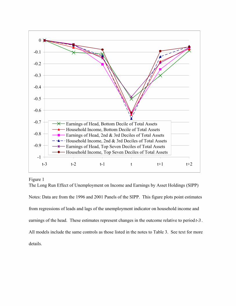
Figure 1The Long Run Effect of Unemployment on Income and Earnings by Asset Holdings (SIPP)

Notes: Data are from the 1996 and 2001 Panels of the SIPP. This figure plots point estimates

from regressions of leads and lags of the unemployment indicator on household income and

earnings of the head. These estimates represent changes in the outcome relative to period t-3 .

All models include the same controls as those listed in the notes to Table 3. See text for more

details.

-1

-0.9

-0.8

-0.7

-0.6

-0.5

-0.4

-0.3

-0.2

-0.1

0

t-3 t-2 t-1 t t+1 t+2

Earnings of Head, Bottom Decile of Total AssetsHousehold Income, Bottom Decile of Total AssetsEarnings of Head, 2nd & 3rd Deciles of Total AssetsHousehold Income, 2nd & 3rd Deciles of Total AssetsEarnings of Head, Top Seven Deciles of Total AssetsHousehold Income, Top Seven Deciles of Total Assets