SUMMABILITY METHODS, SEQUENCE SPACES

AND APPLICATIONS

By

Thomas Emmett Ikard r<

Bachelor of Arts Panhandle State College

Goodwell, Oklahoma 1961

Master of Science Oklahoma State University

Still water, Oklahoma 1963

Submitted to the Faculty of the Graduate College of the Oklahoma State University

in partial fulfillment of the requirements for the Degree of

DOCTOR OF EDUCATION May 1970

"'\,~. -........ ': ....

SUMMABILITY METHODS, SEQUENCE SPACE;-,,,",,

AND APP LI CATIONS

Thesis Approved:

-~Vl J/l~~ Dea-rfcl the Graduate College

11

'•-, .. ....._

"'\,. ~,_,_

PREFACE

Several recent texts which would be appropriate for the three

semester-hour course in real analysis recommended for the General

Curriculum in Mathematics for Colleges by the Committee on the

Undergraduate Program in Mathematics of the Mathematical Ass ocia­

tion of America contain an introduction to the topics of divergent

sequences and summability methods.

This collection of results on summability methods, sequence

spaces, and applications is intended for those students who show an

interest in investigating methods which are more general than conver­

gence by which a number can be assigned to a sequence.

The writer acknowledges his indebtedness to Professors L.

Wayne Johnson and John Jewett, and to each member of the mathematics

faculty for the assistance and encouragement they have given. Pro:.:.

fess or Jeanne L. Agnew deserves whatever credit this work is due.

Her patience and tolerance do not seem to have an upper bound. My

family has lent me the moral support necessary to persevere 1n this

effort, and my wife, Phyllis, has been my greatest help.

111

TABLE OF CONTENTS

Chapter

I. INTRODUCTION.

II. SUMMABILITY METHODS

Sequence -to -function Summability Method Sequence -to -sequence Summability Method K-sequence K-·matrix T-sequence T-m.atrix ~-sequence. '{-sequence.

III. SEQUENCE SPACES

Linear Space Norm ... Metric. . . Linear Metric Space Frechet Space FK-space . . . . . Equivalence . . . . Absolute Equivalence Mean Value Property

IV. APP LI CA TIO NS .

Taylor Series Fourier Series

A SELECTED BIBLIOGRAPHY

APPENDIX

Selected T-Matrices Selected T-Sequences of Mittag-Leffler Type Selected T-Sequences ....... .

lV

Page

1

11

11 14 29 37 40 44 49 55

59

60 63

• 65 70 72 75 83 83 90

93

95 102

l l l

112

113 114 114

CHAPTER I

INTRODUCTION

The topics of infinite sequences, convergence, and infinite

series are introduced in elementary calculus. In most instances diver-

gent sequences and series are not given much attention, Once a

sequence or series is shown to be divergent, it is not usually regarded

as an object of compelling interest, One of the simplest examples of 00

a divergent series is the alternating series Z:: (-1 )n which seems at n=O

first glance to sum nicely to zero if it is written as

00

z:; (-l)n = [ I +(-1)] + [1 +( 9 1)] + ...... :1

n=O

but the sequence of partial sums 1s an oscillating sequence of zeros and

ones and does not converge. This is an excellent example of the fact

that parentheses cannot be inserted or removed with impunity in the

case of a divergent series.

Since the definitions of convergence of a sequence and of the sum

of an infinite series are a way of assigning a number to a sequence,

1;1ome students must wonder if there could be a number between zero

oo n and one which might be assigned to Z:: (-1) in some other natural way.

n=O Some students may discover that the sequence of arithmetic means of

oo n the sequence of partial sums of Z:: ( -1) converges to 1 /2, which is

n=O the arithmetic mean of O and 1.

1

2

In any case, the concept of the limit of a sequence can be

extended for students who wonder about divergent series by an intro-

duction to methods of summability, to the structure of the set of

sequences, and to some applications of methods of summability.

Some of the more prominent mathematicians who have contri-

buted to the theory of divergent sequences and series are Niels Henrik

Abel (1802-1829), Emile Borel (1871-1956), Augustin Louis Cauchy

(1789-1857), Ernesto Cesaro (1859-1906), Peter Dirichlet (1805-1859),

Leonhard Euler (1707-1783), Leopold Fej~r (1880-1959), Jean Baptiste

Joseph Baron de Fourier (1768-1830), David Hilbert (1862-1943), Otto

Holder (1859-1937), Gottfried Wilhelm van Leibniz (1646-1716), Gosta

Mittag-Leffler (1846-1927), and Simeon Denis Poisson (1781-1840).

Comprehensive collections of the theory and applications of divergent

series were written by K. Knopp in 1928 and G. H. Hardy in 1949.

Leibniz and Euler used divergent series in some of their works in

analysis although Abel is reported to have written, "Divergent series

are an invention of the devil, and it is shameful to base any demons tra-

tion on them whatsoever." Perhaps his remark stimulated mathemati-

cians into efforts to make divergent series respectable.

The usual definitions and some theorems which follow readily

from them are listed below for reference or for comparison with

similar theorems concerning summability methods.

Definition 1. 1. A sequence x + = {xn}, n E I of complex numbers

1s a function from I+ into E.

It is Gustomary to write {x } for the sequence rather than n

{ (n, x )} where x = f(n), since the domain of a sequence is always the n n

positive or the nonnegative integers.

Definition 1. 2. Let {a } and {b } be two sequences. These n n

sequences are the same if and only if a n

+ = b for every n E I . n

Definition I. 3, A sequence {a } in E, the set of complex n

numbers, converges to a complex number a if and only if, given any

real number e > 0, there exists an integer N such that n > N implies

/ a - an/ < e. a is called the Emit of the sequence {an}, written

lim a = a. n

Theorem 1. 4. lim a = a and lim a = b implies a = b and n n

a = a for every n implies lim a = a. n n

Theorem 1. 5. Let lim a = a and let limb = b. Then

i) lim ( a + b ) = a + b , n n

ii) lim a b = ab , n n

iii) if c E E then lim ca = ca. n

n n

From the first theorem one can observe that the concept of

3

convergence corresponds to the idea of a function defined on the set of

convergent sequences. The second theorem states that the limit

function is additive, multiplicative, and homogeneous.

The notion of a subsequence is frequently a useful tool.

Definition 1. 6. A subsequence y of the sequence {~}, n E I+ is

a function from I+ into I+ such that y(i) < y(j) if i < j for i, j in I+.

Definition I. 7. If x = {x } is a sequence of complex numbers n ,

and y = {n.} is a subsequence of 1+, then x(y) = {xnJ is called a sub~ 1 1

sequence of~_.

4

Boundedness and monotonicity are also properties which will be

us ef:lJ)!l. in what follows. ;1 .,~

Definition 1. 8. The sequence { a } in E is bounded if and only n

if there exists a nonnegative number M such that /an/ < M for every

+ n E I .

The following theorem is a direct result of the last two defini-

tions.

Theorem 1. 9. Every subsequence of a bounded sequence in E

is bounded.

Since a sequence is a function it can be characterized as mono-

tone increasing or monotone decreasing if it is a sequence of real

numbers.

Definition 1.10. A sequence {a} in R is monotone nondecreas­n

ing if and only if a < a +l for all n e I+ A sequence is monotone non­n - n

increasing if and only if an+l .:::.. an for all n E I+. A sequence is mono-

tone if and only if it is monotone nondecreasing or monotone nonincreas-

ing. A sequence {a } is monotone increasing if and only if a < a +l n n n

+ for all n E I . A sequence { a } is monotone decreasing if and only if n

+ an> an+l for all n E I A sequence is strictly monotone if and only if

it is monotone increasing or monotone decreasing.

The relationships of subsequences and monotonicity is clear

from the following theorem.

Theorem 1. 11. Every subsequence of a monotone nonincreasing

(nondecreasing) sequence is monotone nonincreas ing (nondecreasing).

5

Every subsequence of a monotone increasing (decreasing) sequence is

monotone increasing (decreasing).

Sequences in R have the following important property.

Theorem l. 12. Every sequence of real numbers has a mono-

tone subsequence.

The supremum or least upper bound and the infimum or greatest

lower bound of a set of real numbers are defined next.

Definition l. 13. If AC R then b is the supremum of A, written

b = sup A, if and only if for all a E A, a < b and for any x such that, for

all a E A, a < x then b < x.

Definition I. I:4. If AC R then c is the infimum of A, written

c = inf A, if and only if for all a E A, c < a and for any y such that for ;~i:

all a e A, y .:::_ a then y 2. c.

The completeness of Rand E can be stated in terms of Cauchy

sequences.

Definition 1. 15. ",}

A sequence { an} in E is called i1 Cauchy

sequence (or a fundamental sequence) if and only if for every real

+ number e > 0 the re exists N E I such that / a - a / < e whenever m n

m,n > N.

Theorem L 16. If {a } is Cauchy-in E or in R then lim a n n

exists and is an element of E or R respectively.

Theorem I. 17. The sequence {a} in Eis convergent if and n

only if { a } is a Cauchy sequence in E. n

6

Theorem 1. 18. Every convergent sequence in E is bounded.

Theorem 1. 19. A monotone sequence in R converges if and

only if it is bounded.

There are, of course, sequences in R which are bounded which

are not convergent. Consider the sequence {a } = { 1, 0, 1, 0, 1, 0, ... } n

+ where a 2n = 0 and aZn-l = 1, n e I . It can be seen that the subse- · ~ ,::

quences { a 2n} and { a 2n_ 1} are convergent sequences. This obs erva-

tion is included in the Balzano-Weierstrass Theorem for sequences.

Theorem 1. 20. Every bounded sequence 1n R has a convergent

subsequence.

The concepts of limit superior and limit inferior for sequences

m R are defined next.

that

Definition 1. 21. Let { a }be a sequence in R and let u e R such n

i) for every e > 0 there exists N e I+ such that n > N implies a < u + e, n

ii) for every e > 0 and for every m > 0 there exists n e 1+, n > m such

that a > u - e .. n

Then u is the limit superior of {a } , written u = lim a . The n n

limit inferior of {an}, written lim an' is defined to be -lim bn where

+ b = -a for all n E I . n n

Thus the sequence {a } = {l, 0, 1, 0, 1, 0, ... } has lim a = 1, n n

lim a = 0. The following theorem lists some of the more important n

properties of lim a and lima and their connection with convergence. n -- n

Theorem 1. 22. Let {an} be a sequence m R. Then:

7

i) lim a < lim a • n - n•

ii) { a } converges if and only if lim a , lim a e R and lim a = lim a . n n--n n n

In this case lim a = lim a = lim a . n n n

Infinite series are defined in terms of their sequences of

partial sums and the results for sequences are directly applicable.

Definition 1. 23. Let {a } be a sequence m E, and define n

n

+ 2::: ak' n e I ,

k= 1

The sequence {s } is called an infinite series. The number a 1s n n

called the .!1ih term of the series. The series converges if and only if

{s } converges. n

00 Write 2::: ak for { s } , and if lim s = s, write

k=l n n

00

2::: ak = s. k=l

A series may sometimes be written more conveniently as

00 2::: a and

n=O n

n s = ao + al + 0"" + a = 2::: ak, n n

k=O

Theorem l. 24. Let

00 00

a = 2::: a and b = 2::: b n=l

n n=l

n

1n E, Then for any a,(3 E E,

00 00 00

2::: (aa + f3 b ) = n=l n n

a2:::a +(3 2:::b. n= 1 n n= I n

Theorem 1. 25. Let a > 0 for all n E I+. n-

verges if and only if {s } is bounded above. n

00

Then l: a con­n= l n

8

Theorem 1. 26. Let {a } and {b } be sequences in E such that n n

+ 00 a = bn+l - bn for all n E I . Then l: a converges if and only if

n n= 1 n

limb = b e E. In this case, n

00

l: a n

n=l

co

=limb n

Theorem L 2 7. l: a converges if and only if for every e > 0 n=l n

there exists NE I+ such that n > N implies I a +l + ... + a I < e for n n+p

+ each p e I .

Definition 1. 28. If a > 0 for all n E I+, the series n

1s called an alternating series.

Theorem I. 29. If {a } is a decreasing sequence converging to n

0, the alternating series

converges.

Notice that in the case of the series

co l: (-It+l 1/n

n=l

the sequence of partial sums is the sequence {s } = {l, -1/2, 1/3, ... } n

and

9

(X)

I: (-lt+l 1/n n:: 1

converges by Theorem l. 29. However

(X)

I: /(-l)n+l 1/n/ n::: l

is the harmonic series which diverges. This concept is formalized in

the next definition.

00 if I:

n== l

Definition 1, 3 0.

/a / converges. n

(X)

converges but I: / a / n:: l n

Theorem l. 31.

vergence.

(X)

A series I: a is called absolutely donvergent n:: 1 n

(X)

It is called conditionally convergent if I: a n== 1 n

diverges.

(X)

Absolute convergence of I: a implies con­n== 1 n

The following topics will be used m Chapter IV.

Definition 1. 32. Let z0

e E and let an e E for n e I+ U { O}.

Then the infinite series

or more briefly

is called a power series 1n z - z0

,

Theorem 1. 3 3. Let

n be a power series and let \ = lim ~' r = 1 /\, (where r = O if

n

10

\ = + oo and r = + oo if\= 0). Then the series converges absolutely if

jz - z0

j <rand diverges if jz - z0

/ > r.

The material included in this section is not exhaustive of the

topics to be considered concerning convergence of sequences and series,

but should suffice as a background for what is to follow. Additional

material and proofs of theorems included here may be found in many

books, for example [2 ], [7 ], and [ 10].

CHAPTER II

S UMMABlLlIDxf' 1ME1'ilJHODS: '

The objective of this chapter is to consider methods of assigning

a number to sequences which are divergent. One method, which would

c;ertainly make this investigation a short one, would be to assign each

sequence in E the number 0. This would not produce many interesting

results. One consideration to be kept in mind is that a worthwhile

method of assigning a number to a sequence should not cause a conver-

gent sequence to diverge. In other words, a desirable method should

preserve the property of convergence when applied to convergent

sequences. { l 2.n

If it has become customary to assign the sequence 1+2 }

the number 1, it might be desirable to continue the custom. Thus a

desirable summability method might be required to assign convergent

sequences their usual limits. Some definitions and the ore ms to formal-

ize these concepts and some examples of summability methods follow.

Again let E represent the set of complex numbers, R the set of

real numbers. Let s represent the set of sequences in E, c the set of

convergent sequences in E, and F [(O, oo)] the set of complex functions

defined on (0, oo) C R.

Definition 2. 1. Let {f (x)} be a sequence of functions rn n

F[(O, oo)] and let {z } be a sequence of complex numbers. If n

00

g(x) = 2::: f (i:)z n=l n n

11

12

belongs to F[(O, oo)] and if lim g(x) = t ,:f. oo, then {f (x)} will be called X-> (X) n

a sequence -to-function,;i;um.mabHii:ty: method (or transformation), and

{ z } will be said to be in the domain of {f (x)}. n n

The sequence-to-function transformation {f (x)} operates on the n .

sequence { z } in a way suggested by the inner product of vectors. One n

would define an inner product of vectors in an infinite dimensional

vector space to be the infinite series used to define g(x). For example,

let{z} = {1,0,1,0,1,0,, .. } and let n

{ } { x n} fn(x) = ( 3x+l ) '

Example 2. 2.

{ix~! ' 2

(3x: 1) ' 3

(3x:l) '

x x . x 3 ( )2n-l g(x) = 3x+ 1 + ( 3x+ 1) + · ' · + 3x+ 1 +

(X)

= ~ n=l

= g(x).

(_x ) 2n-l 3x+l

The formula for the sum of a geometric series can be used to write

this in closed form as

g(x) x

= 3x+l

Hence

g(x) = 2

3x +x 2 ' 8x +6x + 1

and { z } is as signed the number lim g(x) = 3 / 8. If { f (x)} = {l /2n}, n x->oo n

13

a sequence of constant functions in F[(O, oo)], then

Example 2. 3.

1 0 1

{t, 1 1 :n , ... } 0 00 21 - 2n

4 ' 8' .. 0 .. j 1 = g(x) = ~

0 n=l

In this instance

g(x) = 1/2 C-~ 14 ) = 1/2(4/3) = 2/3,

and {z } is assigned the number lim g(x) = n 2 /3. Notice that the

x->oo

sequence

{(3x:r} and the sequence {z~} assign the divergent sequence { !, 0, !, 0, !, 0, ... )

two different limits, 3/8 and 2/3 respectively. This is an indication

of the variety which exists when different summability methods are

applied.

It is quite possible that a particular sequence {f (x)} will not n

transform a sequence to a function g(x) e F[(O, oo)] . Consider the

sequence

{f (x)} = {(x~~r} n

Here

00 ( ~) 2n-l g(x) = ~

n= 1 x+l

2x and for x > 1, x+l > 1 so that

00

1:: n=l

14

(~) Zn~l x+l

diverges and g(x) is not defined. Thus in Definition 2. 1 the statement

that g(x) belongs to F[(O, oo)] is not satisfied. In general it is necessary

to assume, whenever the expression

00

g(x) = 1:: f (x)z n=l n n

appears, that {z } is in the domain of {f (x)} and that g(x) is a function n n

in F[(O, oo)J. Care must therefore be exercised in the application of

the definitions and theorems in each particular case.

A case of particular importance arises when the functions

{fk(x)} in Definition 2. 1 are step functions. That is, when fk(x) is

constant on each interval (n-1, n]. Consider the function values at the

right-hand endpoints n. Since the sequence {n} = { 1, 2, 3, ... , n, ... }

is an element of s, the symbol {fk(n)} represents a sequence of

sequences. That is, the continuous variable x is replaced by the

discrete variable n and the set of function values

can be arranged in the rectangular array of an infinite matrix. As

usual, n denotes the row subscript and k denotes the column subscript.

Definition 2. 4. Let (ank) be an infinite matrix of complex

· numbers and let {z } be a sequence of complex numbers. If n

{z' } = n

15

belongs to s, then (a k) will be called a sequence -to -sequence summa ~ n - -~~-- ----

bility method (or transformation), and {zn} will be said to be in the

domain of (ank),

A summability matrix transforms sequences in the same way

matrices transform vectors in a linear space. For example, let

{z} = {l,0,1,0,1,0, ... } and let (a k) = (1/(n+l)k) so that n n

Example 2. 5.

1/2

1 /3

1/4

(a k){z } = n n

1/n+l

1/4

1/9

1 /16

1/8

l/27

1/64

l/(n+l)2

l/(n+l)3

00 co

k 1/(n+l) ...

co

l

0

1

0

1

0

{]] 1 l l 1 = 2k~l'

:z:; Zk~l'

:z:; 4

2k- l '· • ·' :z:; · Zk-1 2 k= I 3 k= 1 k=l (n+l)

2 3 4 n+l ... } = { 3' 8 'Ts'' Q Q O j) n(n+2) 9

= { z' } and lim z 1 = 0. n n

If (a k) is the infinite matrix where a 2 1

= I and a .. = 0 n n, n - lJ

otherwise, and if {zn} = { 1., 0, 1, 0, 1, 0, ... }, then

00}

16

Example 20 6,

1 0 0 0 0 1

0 0 I 0 0 0

0 0 0 0 1 1

(a k)(z ) = n n 0

1

0

so that {z~} = { 1, 1, 1, 0 •• } and lim z'n = L Notice that these matrices

respectively assign the limits O and 1 to {l, 0, 1, 0, 1, 0, 0 0.}, so that

variety is still possible when infinite matrices instead of sequences of

functions are used to transform diver gent sequences.

There are situations where a particular infinite matrix cannot 00

transform a particular sequence since ~ a kz may be a divergent k=l n n

series. Consider the matrix (ank) where ank = 1 for n, k e I+ and the

sequence {z } 1 {l, 0, 1, 0, l, 0, 0 0. }. In this case each series n , 00

~ ankzn is divergenL Again it wiH be necessary to assume whenever k=l { z i } is written as

n

{z } are such that n

00

{ ~ a kz } that the matrix (a k) and the k= 1 n n oo n

each series ~ a kz is convergent, and k=l n n

sequence

to use

caution in applying definitions and theorems to particular sequences

and matrices.

The lemmas which follow are required for the proof of a f~nda-

mental theorem concerning summability methods. It will become

evident that the proof is not short or easy. Shorter proofs using the

methods of functional analysis are given in [11] and [13].

17

Lemma 2. 7, Let {f (x)} be a sequence of functions in F[(O, oo)] n

+ such that lim f (x) = a f. oo for every n e I , ,: Then if there exists an x-+oo n n

x0

E (0, oo) and there exists Me (0, oo) such that

00

00

;[;

n=l !f(x)i<M

n

for all x > x0

> 0, then ;[; a is absolutely conve rgenL n= 1 n

Proof: lim f (x) = a -f. oo for all n e I+ implies that for every x-+oo n n

positive number e and each integer p e I+ there exists x, depending on

n, written x(n) > 0 such that if x > x(n) then / a - f (x) / < e/p, Since n n

la I - /f (x)I < /a -f (x)/ <e/p, it follows that la I< /f (x)I +e/p n n - n n n n

whenever x > x(n),

Now

00

;[;

n=l /f(x)l<M n

for all x > x0

> 0 implies that

p ;[;

n=l 1£ (x) / < M n

+ + for every integer p e I whenever x > x0

. Given any p e I ,

p p 2: /a I< 2: (/£ (x)/ + e/p)

n= l n n= l n

for x > max {x(l).,,, ,x(p)}. or

p 2: la /<M+e

n= I n

for x > max {x0

, x( l ). , , , , x(p)}, Thus for each p e r+, p 2: /an/ :::_ M + e'

n=l

18

00

and the sequence of partial sums of ~ n=l

/a I n is bounded. This proves

the lemma.

The next lemma concerns the behavior of a divergent sequence.

00 Lemma 2. 8. If ~ / u / is divergent, then there exists a

n= 1 n

sequence { z } in E where lim z = 0 and n n

1s not bounded.

since

ic/>

Proof: Let un :::: / un I e n and choose a real number r > l. Then

00 + ~ / u / is divergent there exists p

0 e I such that

n= l n

Po ~

n= l /u I > r. n

2 + Now r > l implies r > r > l and there exists p

1 E I such that

lu I> n

2 r .

3 2 + Similarl.y we have r > r > r > 1 and there exists Pz e I such that

lu I> n 3

r '

Let -ir.Dn z = e for l .'.'.::. n .'.'.::. Po, n

~ir,6 e n for :::: Po < n .'.'.::. P1 • r

-ic/> e n

= -2- for P1 < n .::_ Pz, ... r

Note that lim z = 0 and that n

oo Po ~ u z = ~

n= 1 n n n= l

>r+r+r+

and the lemma is proved.

.... '

lu I+ l/r2 n lu I + 0 •• n

The following lemma discuss es the pr ope rtie s of an infinite

matrix whose rows and columns obey certain conditions.

Lemma 20 9. Let (snk), n, k e I+ be an infinite matrix of real

numbers and let lim s k = bk for all k E I+ 0 If n ..... oo n

+ for every n e I , then the sequence

s n

{ ~ Is kl} k=l n

+ is bounded £or each fixed p E I .

Proof: The matrix is exhibited in Figure 2. IO

s 11 812 s 13 ·C;

~lp ~ Is rk ! 8

21 8 22 8

23 s2p ~ ls2kl 8

31 8

32 8

33 s3p ~ I s3k I s s

n2 s

n3 s ~ /snk! nl np

t b

p

Figure 2 0 l.

= s l

= sz

= s3

= s n

19

The hypothesis that lim s k = bk justifies the appearance of n-->oo n

20

column limits in the diagram. Further, lim s k = bk implies that for n ... m n

+ every positive number e and for each fixed integer p e I there exists

N(p) e I+ such that if n > N(p) then I snk ~ bk I < e/p. Hence

I snk I < lbk I + e /p and

In Figure 2. l this states that partial sums along the nth row are

,bounded by partial sums of the column limits for rows sufficiently far

down in the array.

Now let us consider the rows above the (N+l)st row and the

columns through the pth column. In this rectangular array in the

upper left-hand corner of the diagram,

so that

~ Is I< ~ p . ( p

k= 1 nk k= l

N ~

n=l

where l is added to insure strict inequality. Therefore the partial

row sums above the (N+l )st row are still bounded by the sum of the

elements in then Xp rectangular array in the upper left-hand corner

of the diagram plus one.

Suppose that

+ is not bounded for some fixed p E I , then for each M > 0 there exists

j e I+ such that

Let

p ~ jsJ.k! > M.

k=l

Mc max h /bk/ G=l

+ e, N ~

n=l

Now if j > N, then

and if 1 ~j ~N, then

p

< ( ~ N

/snk/) + I :',M ~ is.kl ~

k=l J k=l n= l

which is a contradiction. Hence for each fixed p E I+ there exists

M > 0 such that p

+ for all n E I .

In the case that

{ ; is kll k=l n J

is not a bounded sequence, the next lemma exhibits a convergent

sequence {xk} such that the transform of {xk} by (snk) diverges.

Lemma 2. l 0, If

21

for all n e I+ and {sn} is not bounded, then there exists a sequence {xk}

such that lxkl ~ 1 fork.er\ Um xk = 0, and

{x'} = [; s x } n l k= 1 nk k

has a subsequence {x'n_.} which diverges. 1

22

Proof: If {s } is not bounded then for every r > I there exists n

n1

and q1

in I+ such that

Otherwise,

q I ~

k=l

2 r .

2 < r

for every q1

and n1

E I+ would imply that sn1

< r2

for all n1

E I+, so

that { s } is bounded, contrary to hypothesis. n

Let e > 0, then there exists N E I+ such that

whenever m > N. Hence

whenever m > N. Now

implies that

I sn ~ 1;? / s k I I < e k=r n I

m s

n - ~ /s kl < e k=l n

00

~

k=l

00

s n

~ I snk I < e k=m+l

whenever m > N. Thus there exists an integer p1 ~ q

1 such that

co ~ Is k/<eo

k=p1 +l n 1

Now the first p1

terms of {xk} may be defined as follows,

=

=

x = P1

Notice that

and that

/snlpl/

rs nlpl

if s l -/:- 0, x I = 0 if nl

if s 2

i 0, nl

if s nlpl

j 0, x = 0 P1

/sulk/

=L if s k>O

nl s

n1

k if s k < 0

nl

if s nlpl

/ snl k / for l~k~p 1o s x = n

1k k r

= Oo

Now consider the transform of the first p1

terms of {xk} by the n 1st

row of (snk),

Also

P1 I

~ /s k/>ro r k= l nl

23

if sn1

k-/:. 0 and lxk/ = 0 ifsn1

k = 0 so that /xk/ < 1 for l .:::_k.:::_pl"

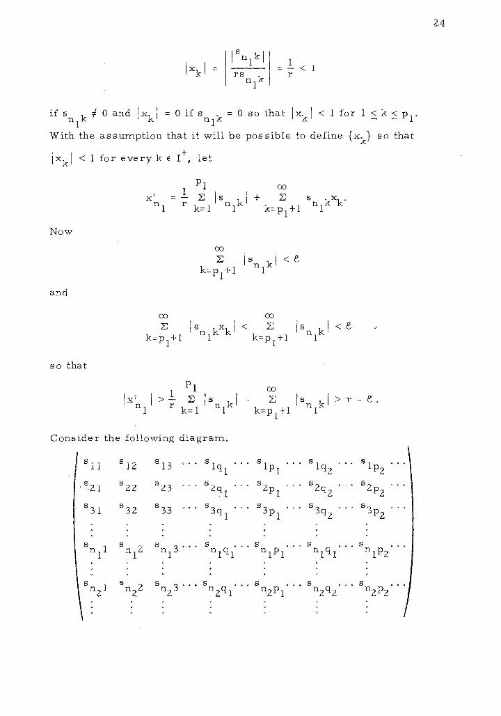
With the assumption that it will be possible to define {xk} so that

jxkj < 1 for every k e r\ let

Now

00

~ Is kl < e k=p

1 + 1 n 1

and

so that

Consider the following diagram.

8 11

812 813 8

lql s

lpl s

Iq2 s

Ipz

'8 21 8

22 8

23 82 s 8 s ql 2pl 2q2 2p2

831

832

833

s s s s3 3ql 3pl 3q2 Pz

8 n

11

s n?

s n1

3 · · · s ... s s s nlql nlpl nlql nlp2

s nzl

8 n

22 s n

23 · · · s s s s

n2ql n2P1 n2q2 n2Pz

2.4

25

The subscripts n1

and p1

have been used to define the first p1

terms of

{xk} and the first term x' of a subsequence of nl

Now choose the distinguished subscripts n2

> n1

and q_2

> q1

such that

q2

_!_2 ~ I s k I > M + r2' k 1 n2 P 1 r =pl+

where M is the upper bound for P1

which is provided for in Lemma 2. 9. Next choose the subscript

Pz ::::_ q 2 such that

00

~ Is kl<e k=pz+l n2

Now define xk for p 1 < k .:::_ Pz as follows:

x = Pz

Again notiGe that

if s t- 0, nzPz

x = 0 if Pz

s = 0 • nzPz

for p 1

< k ~ p 2

, and that

= _l_ < 1 2

r

for p 1 < k ~ Pz· The transform of the first Pz terms of {xk} by the

n 2 th row of (snk) is

Again assume that lxkl < 1 for all k EI+ and define

Now

P1 Pz .!.. "" + l ""

£..../ snzkxk -2 £..../

r k=l r · k=p1

+1

> Pz

_l_ ~ 2

r k=p 1+1 Is k I n2

Thus since /xkl < l for l ~k~p 1 ,

and

2 orlx' l>r -e.

nz

P1 l ~ s x < M r k= l n 2k k p 1

- e

- e,

- e.

26

27

Continuing in this fashion, for each k e I+ there exists n e I+

such that I xk I < r -n and lim xk = 0. In addition for each i and each k

in I+ there exists n. in I+ such that /x1n I > rk. Thus {x 1 } diverges

i i - ni

and the lemma is proved.

To illustrate Lemma 2 1 10, consider the infinite matrix (snk)

k where s lk = l /2 and

- (n-l)k-1 snk - n

for n > l, as in the diagram below.

l /2

1

1

1

l

l / 4

1/2

2/3

n-1 n

1

1/8

1/4

4/9

1

l/2k L Is ik I

l/2k-l L I s2k I (2/3)k-l L I s3k I

~ )

k-1 n-1

n

1

Let r = 2 so that integers n1

and q1

must be found so that

ql

If n 1

= 8 and q 1

= 6 then

6 L (7 /8t-l =

k=l

L Is k I > 4. k= 1 nl

l -(7 /8)6

= 1-7/8 (

'144, 495) 8 262, 144 > 4 · 4 ,

= 1

= 2

= 3

00

28

using the formula for the sum of n terms of a geometric progression.

Following the pattern of Lemma 2. 10, let e =l so there must be an

integer p1

:::._ q1

= 6 so that

00

~ (7 /St-I < 1. k=p1+1

If p 1 = 20 then

~ (7/st-i= s -7 >7.4 20 ( 20 20)

k=l s 19

and

00

~ (7 /8)k-l < . 6 < L k=21

This means that xk = 1 /2 for 1 .:::_ k .:::_ 2 0, and that

x 1 =l/2(7.4)+.6=4.3>r-e=2-l=l. nl

In the next part of the lemma, n2

and q2

must be chosen so

that n2

> 8 and q2

> 20 and at the same time

or q2 (n -1 )k- l ~ 2

> 4 M 2 O + 16 . k=2 l n2

Note that M20

, which is the maximum term of

is less than or equal to 20. Hen,_ce n2

and q2

must be such that

Jtz:/ rl > 96.

Now

20 (l 24)k- l ~ 125 < 20 ,

k= 1

so let n 2 = 125 and let q2

= 340. Thus

\~ 0 ( 12 4) k - 1 - 1 0 0 k=21 125

and p2

::_ 340 can be chosen so that

00 (124)k-l ~ \125 < 1.

k=p2+1

This gives xk = 1 /4, 20 < k :::_ p2

and

/x' />20+4-20-1 n2

2 =2 -e=3.

Continuing in this fashion, lim xk = 0 and { / x~. /} is not bounded. 1

Now the conditions under which a summability transformation

29

will transform convergent sequences into convergent sequences can be

examined.

Definition 2. 11. Let f (x) be a sequence-to-function summa­n

bility method. If

00

g(x) = ~ f (x)z n=l n n

belongs to F[(O, oo)] and if lim g(x) = t f. oo for every convergent x-100

30

sequence {z } in E, then {f (x)} is a conservative sequence-to-function n n

s umma b ili ty method. In this case {f (x)} will also be called a Kojima n

sequence or a K-sequence.

The following theorem 1 which gives necessary and sufficient

conditions that a sequence {f (x)} should be conservative, was proved n

by Kojima in 1917 and extended by Schur in 1918. Its present form is

the result of further extension and refinement by Agnew, Cooke, Hardy,

and others.

Theorem 2. 12. (Kojima~Schur) Let{£ (x)} be a sequence-to­n

function summability method. Then { f (x)} is a K ~sequence if and only n

if:

i) there exists x0

e (0, oo) and there exists Me (0, oo) such that

00

ii)

2:: /fn(x)/ .:::_M, forallx>x0

>0, n=l

lim f (x) n x-+oo

00

= a I- oo for all n e 1+, n

iii) 2:: f (x) = f(x) and lim f(x) = a I- oo. n= l n x -+oo

In this case

lim x-oo

where lim z = z. n

g(x) = lim x-oo

00

2:: f (x)z n=l n n

00

= az + 2:: a (z - z) n=l n n

Proof: a) The three conditions are sufficient.

Let {z } be a convergent sequence, that is, let lim z = z. This n n

means that for all positive real numbers Mand e, there exists N 1

e I+

such that / zn - z I < e/3M whenever n > N 1

. Let

31

k = max { j zn - z j : 1 :::_ n :::_ N 1},

00

From conditions i and ii, and Lemma 2. 7, ~ a 1s absolutely n=l n

convergent, Hence, there exists an integer N2

such that

/a I :::_M, n

for every positive number M.

Choose N = max {N 1, N2 } and consider / fn (x)- an j, where

1 < n < N. + From condition ii, there exists x 1 e R such that

whenever x > x 1• Hence

for x > x 1 •

These bounds for I zn - z /, 1 :::_ n :::_ N 1

; for

and for

N ~

n=l If (x) - a I, n n

x > x 1 will be used to show that

00

lim ~ f (x)( z - z) = n=l n n X--+ 00

Condition i implies that

co ~ a (z ~ z).

n=l n n

co ~

n=N+l If (x) I < M

n

whenever x > x0

> 0. Now let x = max {x0

, x 1} and write

co ~ (£ (x)-a }(z -z)

n=l n n n

N oo = ~ (£ (x)-a }(z -z) + ~ (£ (x)-a )(z - z)

n=l n n n n=N+l n n n

<

+

N co ~ jf (x)-a llz -zl+ ~ jf (x}llz -zl

n=l n n n n=N+l n n

co ~

n=N+l ja llz - zj. n n

With N chosen, and with x > x,

32

co ~ (£ (x)-a )(z - z)

n= 1 n n n < 3 (k+ 1) (k+l}+M · 3~ +M· 3~ =e.

Hence

co co lim ~ f (x)(z -~ z) = ~ a (z - z),

n= 1 n n n=l n n X-, 00

and

co co co lim ~ f (x)z - z

n=l n n lim ~ f (x) = ~ a (z - z).

n= 1 n n= 1 n n x- co x--, co

Condition iii implies that

lim x-co

since

co co ~ f (x)z - za = ~ a (z - z),

n= 1 n n n= 1 n n

lim x --,co

co ~

n=l f (x) = a. n

Now if

converges, then

00

L a (z - z) n=l n n

00

lim L f (x)z n=l n n x-+oo

will exist as a finite number in E. Now

00

co L

n=l Ja l=t-loo n

33

since L a is absolutely convergent and J z J < r -I oo since lim z = z, n=l n n n

Also I zn - z I .:::_ j zn J + I z J < r + J z J, and therefore,

so thc1,t

00

L n=l

I a 11 z - z I n n

00

< L n=l

la j(r+ lzl) = (r+ lzf)t, n

00

L n=l

a (z - z) n n

is absolutely convergent, Thus

is convergent and

00

lirrt L f (x)z n= 1 n n x-+m

a finite number in E,

00

L n= 1

a (z ~ z) n n

= lim g(x) = x--+oo

00

az + L a (z - z ), n=l n n

This proves that 1, ii, and 111 are sufficienL

b) The three conditions are necessary,

34

Lemma 2. 10 will help to show that condition i is necessary.

Suppose condition i is not satisfied. That is, suppose that given

x e (0, oo) and given Me (0, oo) there. exists x0

> x such that

00

:E I fn(xo) I > M. n=l

Let.£ (x) = u (x) + iv (x), where u (x) and v (x) are re.al. Then there n n n n n

exists a sequence { y } such that limy = x0

and there exist sequences . n n

{ s } = ) ; I uk ( y ) IL and n lk=l n j { t } = f; I vk(y ) 1}

n lk=l n

such that for every M > 0, either lim s > Mor lim t > M. Suppose n n

that for every M > 0, lim sn >Mand write snk = uk(yn), so that

s n

Lemma 2. 10 shows that there exists a sequence {xk} which converges

to zero, but the sequence

has a subsequence {x'n.} which diverges. This means that if condition 1

i is not satisfied then there is at least one convergent sequence which

is transformed by {f (x)} into a divergent sequence. Thus condition i n

is necessary.

For the second condition, let z = 0, n f. p and let z = 1 if n = p. n n

Then lim z · = 0 and g(x) = f (x) $0 that lim i (x) = a f. oo for all n p x .... 00 n n

·+ n E I is necessary for lim g(x) = z0

f. oo. x-+oo

35

In the case of condition iii, let z = 1, n e I+ so that lim z = 1. n n

Then

CD g(x) = ~ f (x),

n=l n

and therefore,

CD ~ f (x) = f(x),

n=l n

where lim f(x) = a I- oo, is necessary for lim g(x) = z0

I- CD. x-oo x-CD

This proves the the or em.

Example 2. 13: An example of a K-sequence is the sequence

{ { [ -x 2 2] -1 f(x)}= (e +l) +n }. n

Here

and it can be shown that

CD ~

n=l /£ (x)/ = 'IT -x 1

coth rr(e +l) -n

Thus,

and

for x e (0, CD). Also

CD ~

n=l If (x) / < ~ c oth 2,r -

1 n - 2 8'

00

~

n=l / f (x) / < M

n

[ -x 2 2] -1 lim f (x) = lim ( e + l) + n

n x-CD x-CD

for all n e I+.

2(e-x+l) 2

Last,

lim ~ f (x) = lim 'TT coth [ ,r( e -x + 1)]

x ..... oo n= 1 n x ..... oo 2 ( e -x + 1)

1

'TT 1 = z coth 'IT - z

This means that if lim z = z then n

lim g(x) = lim r ¥- coth 'TT - -}] z x .... oo x-100L

Let

so that lim z = 0 and n

2 {z } = { .!±~}

n Zn

lim g(x) = X_,00

00 ~

1

n= 1 Zn = 1.

00 z -z + ~ n

n= 1 1 +n2 .

36

Example 2. 14, AK-sequence which transforms every conver-

gent sequence into a sequence which has the limit zero is the sequence

Here

(X)

~

n=l I£ (x) I n

{fn (x)} = { 2 1

2 2} · x +4n n

00 = ~

n=l

1 2+4 2 2 x n 'TT

from results in the theory of functions of a complex variable, and

whenever x > 10 > 0.

00 I ( 4 I ) ~ / fn (x) / ~ 20 To + IO

n= 1 e - I

In this example, lim f (x) X_,00 n

+ = 0 for all n e I and

q:> lim ·~ f (x) = 0.

n=l n

Hence

x ..... (X)

(X)

lim g(x) = lim [Oz + ~ x->oo x-+oo n=l

for every convergent sequence {z }. n

O(z - z)] = 0 n

37

Now that the notion of K-sequence has been characterized, the

same scrutiny can be applied to infinite matrices. The next definition

and theorem will do this.

Definition 2. 15. Let (ank) be a sequence-to-sequence summa-

bility method. If every convergent sequence { z } in E is in the domain n

of (ank), and if

lim z 1 = n

lim n ..... oo

t =f. (X)'

then (a nk) is a conservative sequence -to -sequence summability method.

In this case (ank) will also be called a Kojima matrix or a K-matrix.

Theorem 2. 16. Let (ank) be a sequence-to-sequence summa-

bility method. Then (ank) is a K-matrix if and only if:

i) there exists n0

1: I+ and there exists Me (0, oo) such that

ii)

00 ' + n:l Jank/< M for every n > n 0 > 0, ne I,

lim a k = bk =f. oo for every fixed k e I+, n->oo n

00

iii) ~ a k = r k=l n n

and lim r = a =f. oo. n

In this case

lim z 1 = lim n n ..... oo

00 00

~ ankzk = az + ~ bk(zk - z) k= I k= 1

where lim z = z. n

Proof: Let n, k e I+ and for n - 1 < x ~ n define fk(x) = ank"

This means that the rows of (ank) correspond to a sequence of step

functions in F[(O, oo)J. Thus condition i holds if and only if

for every x > n0

. Next, condition ii holds if and only if

x-> (X) n ->oo

+ for every k e I . Lastly, condition iii holds if and only if

(X)

~

k= I a = r

nk n

and lim r = a f: oo. Thus Theorem 2, 16 is a special case of the n

Kojima- Schur theorem. This means that

(X)

lim ~ fk(x)zk = lim x _, oo k= 1 n ..... oo

(X)

~ a , zk k= 1 UK

00

= az + ~ bk(zk- z) k=l

= lim z 1

n

whenever lim z = z, and the theorem is proved. n

Example 2. 17. The matrix

(a ) = (~) nk nZk

is an example of a K-matrix, since

38

39

3n-l <4

n

+ for all n e I and since lim (3n-l)/n = 3. Also,

lim 3n-l 3

= n2k 2k n-'>OO

for all n E I+. Here the characteristic numbers are ak = 3 /2k and

a= 3. In this case the transform of a constant sequence will converge

to three times the constant. The sequence {z} = {l,O,l,0,1,0, . .,} n

2(3n-l) . is transformed by (ank) into the sequence { 3n } which converges

to 2.

Example 2. 18. The matrix (ank) = 2-k is a K-matrix because

00

~ 2 -k = 1 k=l

for all n e I+, and lim 1 = 1. Here lim 2-k = 2-k, and the character­n .... oo

-k istic numbers of (ank) are ak = 2 and a= 1. The sequence

{z} ={l,O,l,0,1,0, ... } is transformed into the sequence n

{2/3, 2/3, 2/3, .. ,}, a constant sequence with limit 2/3.

Notice that Theorem 2. 16 and Theorem 2. 12 not only charac -

terize K-matrices and K-sequences, but they also state the relation-

ship between lim z if { z } e c and lim z 1 where {z 1 } is the transform

n n n n

of { z } . The numbers a and a in Theorem 2. 12 and the numbers a n n

and bk in Theorem 2. 16 are called respectively the characteristic

numbers of the K-sequence {f (x)} or the characteristic numbers of n

the K··matrix (ank) because of their role in determining the value of

the transformed sequence.

40

The next definitions and theorems are concerned with sequences

{fn(x)} and matrices (ank) which assign convergent sequences their

usual limits.

Definition 2. 19. Let {f (x)} be a sequence-to-function summa­n

bility method. If every convergent sequence {z } in E is the domain n

of {f (x)} and if n

00

lim g(x) = lim X ... CD X ... 00

L f (x)z = z n=l n n

whenever lim z = z, then {f (x)} is a regular sequence-to-function n n

summability method. In this case {fn (x)} will also be called a Toeplitz

sequence or a T-sequence.

The following theorem concerning T-s equences was first proved

by Toeplitz in 1911, extended by Silverman in 1913 and by Schur in

1920.

Theorem 2, 20. (Toeplitz-Silverman) Let {f (x)} be a sequence­n

to-function summability method. Then { f (x)} is a T-s equence if and n

only if:

i.) there exists x0

E (0, oo) and there exists M E (0, oo) such that 00

n:l ifn(x) I .:::, M, for all x > x 0 > O,

ii) lim f (x) = 0 for all n E I+, X ... 00 n

00

iii) L f (x) = f(x) and lim f (x) = 1. n=l n x ... oo

In this case 00

lim g(x) = lim X_,CD X--,00

L f (x)z = z n=l n n

whenever lim z = z I: oo. n

41

P:i;oof: a) i, ii, and 111 are sufficient. Let a = 1 and a = 0 m n

Theorem 2. 12 so that

00

lim g(x) = lz + ~ O(z - z) = z. n=l n X->OO

b) i, ii, and iii are necessary. Since every T-sequence is a

K-sequence, and condition i is necessary for {£ (x)} to be a K­n

sequence, then condition i is necessary for {f (x)} to be a T~sequence. n

Let z = 0 ifn I: p and let z = 2. In this case lim z = 0 and n p n

00

~ f (x)z = 2£ (x), n= 1 n n p

This will. be zero only if lim f (x) = 0. Hence condition ii is necessary. X->00 p

Let z = 1 for all n e I+. In this case lim z = 1 and n n

00 00

~ f (x)z n=l n n

= ~ f (x). n=l n

This will be one only if condition iii is satisfied, This proves the

theorem.

Example 2. 21. The Mittag .,Leffler sequences are a collection

of T-sequences where

{£ (x)} = {g(n) xn-llI n E(x)

such that g(n) ~ 0, g(n) > 0 for infinitely many integers n e /, and

E(z) 00

n·· I = ~ g(n)z n=l

is an entire function. That is, E(z) is analytic rn the finite complex

plane. Now

so that

Also

Now

so

1im x-+.~

00

z:: n=l

If (x) I = n

00

z:: n=l

n-1 g(n)x

E(x)

lim x->oo

lim f (x) n

x ->oo

= 1

E(x)

00 n-1 Z:: g(n)x

n=l

1 = E(x) · E(x) = 1,

00

Z:: f (x) = 1. n=l n

n·-1 x = g(n), lim E(x) . x->oo

= ( ; g(k)xk-n k=l

n +-x­

n-1 x

00 k-1)-1 Z:: g(n+k)x k=l

n-1 x . E(x)

= (M + lim x: ~ g(n+k)xk·-l)-\ O x _, oo k= 1

since g(n) > 0 for infinitely many n E I+.

Example 2. 22. A particular Mittag-Leffler sequence is the

Borel sequence,

{f (x)} n

For the Borel sequence,

42

(X)

~ £ (x) n=l n

Now

lim £ (x) n x ->(X)

Hence

(X)

= ~ n-1

x x

n= 1 e (n-1) !

= 1

lim (X) _(n-1) ! x ->(X) ~

lim x ..... (X)

(X)

~

n=l

k=l

£ (x) = 1 n

1 k-n+l =

x (k-1 )!

+ and lim £ (x) = 0 for all n e I . Consider the sequence X->(X) n

{ z } = { 1, 0, 1, 0, 1, 0, ... } . Then n

and

(X)

~

n=l

(X)

£ (x)z = ~ n n n= 1 ex(2n- l) !

= e -x sinh x

lim -x

e sinh x = 1/2. x .... (X)

o.

so that { 1, 0, 1, 0, 1, 0,.,.} is assigned the limit 1 /2 by the Borel

sequence.

Example 2. 23. If g(n) = (2n-2)! when n = 2k-l, and g(n) = 0

when n = 2:k then

Thus,

oo 2n-2 E(z) = ~ -,--,z=-----=-c~

n= 1 (2n-2 )! = cosh z.

n-1

{fn(x)} = { coshxx (2n-2)!}

and if {u } = { 1, -(2), 4/2, -6/3, ... } then n

43

(X)

Z: f (x)u n= I n n

= I cosh x

O'.)

z: n=l

(-xt- l = (n-1)!

1 cosh x

I x

e

44

so that lim g(x) = 0. Note that, for this choice of g(n), the sequence x ..... O'.)

{f (x)} is quite powerful! n

The next definition and theorem characterize T-matrices.

Definition 2. 24. Let (ank) be a sequence-to-sequence summa-

bility method. If every convergent sequence {z } in E is in the domain n

of (ank)' and if

O'.)

lim z 1 = lim Z: a kzk = z n n ...., oo k= 1 n

whenever lim zn = z /. oo, then (ank) is a regular sequence-to-sequence

summability method. In this case (ank) will be called a Toeplitz

matrix or a T-matrix.

Theorem 2. 25, Let (ank) be a sequence-to-sequence summa­

bility method. Then (ank) is a T-matrix if and only if:

i) there exists n0

E I+ and there exists ME (0, m) such that

~ /ankj .:::,Mforeveryn>n0 >0, ne 1+, n=l

ii) lim ank = 0 for every fixed k E 1+, n .... oo

(X)

iii) Z: a k = r k=l n n

and lim r = 1. n

In this case

lim z 1 = n

where lim z = z. n

lim n...., m

(X) CQ

Z: a kzk = 1 z + Z: 0 ( zk- z) = z k= I n k= 1

45

Proof: a) i, ii, and iii are sufficient. Let a = 1 and bk = 0 in

Theorem 2. 16 so that

lim z 1

n

co = 1 z + ~ O(zk - z) = z.

k= 1

b) i, ii, and iii are nec;essary. Since every T~matrix

is a K-matrix, and condition i is necessary for (ank) to be a K-matrix,

then condition i is necessary for (ank) to be a T-matrix.

Let zk = 0 if k "f p and let zp = 'TT. Then

Here lim z = 0 and n

co ~ a kzk = 7ra

k=l n np

co ~ a kzk = 7ra

k= 1 n np

Now lim na np

= 0 only if lim a n .... co np

= 0. This means that condition ii n .... co

is necessary.

Now

Let z = I for all n e I+ so that lim z = 1 and n n

00

~ a kzk = k=l n

lim n .... co

00

~ a k' k= 1 n

will be one only if condition 111 is satisfied, and the theorem is proved.

Exam:ele 2. 26. An example of a T-matrix is the matrix (ank)

where ank = 1 /n if k .:::_ n and ank = 0 if n < k. This matrix is called

the matrix of arithmetic means. For this matrix,

46

n 1 = 1

for all n E I+ and lim a k = n-+oo n n-+oo n

lim 1

= 0 for all k e I+. Hence its

characteristic numbers are ak = 0 and a = 1. This matrix transforms

{z } = {l, 0, l, 0, 1, 0, ... } into the sequence n

1 2 1 2 1 {l, 2' 3' 2' · .. ' 2k-l '2' · "}

which has the limit 1 / 2.

Example 2. 27. The matrices of Cesaro means of order r > 0

are a family of T-matrices where

a = nk

if k < n and a k = 0 if n < k. - n

rr(n+l)r(r+n-k) r (n-k+ 1 )r ( r+n+ 1)

Here

r (x)

and r(n) + =(n-l)!forneI. Note that rr(r) = r(r+l). Thus

00 n rr(n+l)

n r (r+n-k)

lank! '.\'\

~ = ~ a = E k=O k=O .

Consider

1

(l··Z)j+l

and

I

(1-z)m+l

nk r(rt.1'.i+J) k=O

= ~ r(j+n+l) n=O r(j+l)r(n+l)

r(n-k+l)

n z '

= ~ r(m+n+l) zn n=O r(m+l) r(n+l)

whenever j z I < 1. Then

(1-z)j+l (1-z)m+l =

CX) ~ f'(m+j+n+2) zn

n=O f'(m+j+2)f'(n+l) 1 1

h · f h ff' · f n - k k so t at 1 t e coe 1c1ents o z · z = n

z are equated,

n ( r(j+n-k+l) f'(m+k+l) ) f'(m+j+n+2) k:o f'(j+l)f'(n-k+l) · f'(m+l)f'(k+l) = r(m+j+2)f'(n+l)

Now let m = 0 and let j = r-1, then for r > 0,

n ~ f'(r+n-k) f'(r+n+l)

= k=O f'(r)f'(n-k+l) f'(r+l)f'(n+l)

Hence,

n r f'(n+l )f'(r+n-k)

k:o f'(r+n+l)f'(n-k+l)

and ak = 1 for all k E I+. It can be shown that

= 1,

n+ -ik: -n .J..2 q(n) f'(n+l)=n "'e 2rr e

where lim nq(n) = 0. This means that n _., oo

1. f'(r+l)f'(n+l)f'(r+n-k) im f'(r)r(n-·k+l)f'(r+n+l)

n ->oo

= r lim ll""'OO

r(n+l)f'(r+n-k) r (n-k+ 1 )f'( r+n+ 1)

47

= r lim n...., oo

n+i -n2 i q(n)( + k l)r+n-k-! -r-n+k+l 2 1a; q(r+n-k-1) n e rr e r n - - e 'IT"' e

= re lim n...., oo

( k)n-k+ ! -n+k 2 ! q(n-k) ( + )r+n+! -r-n2 ! q( r+n) n- e rr e r n e rr e

= re lim n ->co

= re lim n -+co

= 0

48

(~)n+! (r+n-k-l)n-k+i (r+n-k-1) r ( 1 ) r+n n-k r+n r+n-k-1

(~ ~ )n+! (1 + E.:...!-) n-k+! (1 - k+l )r ( 1 )

1 n-k r+n r+n-k-1

n

for all k < n and for all r > 0, so that a= 0 and the Cesaro matrices of

all orders r > 0 are T-matrices. If r = 1, then ank = 1/(n+l) if k ~ n

and ank = 0 if n < k so that the sequence {zn} = {l, 0, 1, 0, 1, 0, ... } is

transformed into the sequence { 1 /2, 1 /3, 1 /2, ... , 1 /2, k/(2k-l), ... }

whose limit is 1 /2.

For every sequence {x } in E there.is an associated infinite n

co series k~l ck where c 1 = x 1 and ck= xk- xk-l if k > 1. Thus n co L ck = x , and { x } is the sequence of partial sums of L ck. This

k= 1 n n k= 1

means that the results on sequence -to -function transformations can be

extended to theorems on series -to -function transformations.

Definition 2. 28. + Let hk(x) e F[ (0, co)] for all k E I , and let

co L ck be an infinite series of complex numbers such that

k=l

co g(x) = L hk(x)ck

k= l

belongs to F [(O, co)]. If lim g(x) = t f:. co, then {hk(x)} will be called x-+co oo

a series -to-function summability method, and L ck will be said to be k= 1

in the domain of {hk(x)}.

Just as before, care must be exercised in the application of this

definition to particular sequences {hk(x)} and to particular series

49

00 00

~ ck since ~ hk(x)ck may not converge to a function in F [(O, oo)J. k= 1 k= 1

Conservative and regular series -to -function transformations

are defined in a manner analogous to that for conservative and regular

sequence-to-function transformations.

Definition 2.29. Let {hk(x)} be a series-to-function summa­

bility method. If

00

g(x) = ~ hk(x)ck k= 1

belongs to F [(O, oo)] and if lim g(x) = t f. oo for every convergent series 00

x-->oo

~ ck in E, then {hk(x)} is a conservative series -to-function summa­k= 1 bility method. In this case {hk(x)} will also be called a @ -sequence.

Definition 2. 30. Let {hk(x)} be a series-to-function summa-

bility method, If

00

g(x) = ~ hk(x)ck k= 1

00

belongs to F[ (0, oo)] for every convergent series ~ ck = t m E 1, and k= 1

if

lim x-->oo

00

g(x) = ~ ck = t, k=l

then {hk(x)} is a regular series -to-function summability method. In

this case {hk(x)} will also be called a -y-sequence.

The following lemma, first proved by R. Henstock, will be used

in the proof of a theorem for series -to·-function transformations which

is the analogue of Theorem 2. 12.

Lemma 2.31. Let {gk(x)} be a sequence of functions in 00

F[ (0, oo)] such that for every convergent series ~ ck in E, there

50

k=l exists x 0 e R + such that ]

1 gk(x)ck converges for every fixed x > x

0 > 0.

Then there exists a real number M(x) for each fixed x > x0

> 0 such

that I gk(x) I ~ M(x) whenever k e r+.

Proof: Suppose the lemma is false, that is, suppose that for

every r E I+ there is an x > x0

s.uch that {gk(x)} has a subsequence

{gk (x)} where /gk (x)/ > r2

. Let ck= 0 if k f. kr; let r r

= 2 r gk (x)

r

if gk (x) f. O; and let ck = 0 if gk (x) = 0. r r r

Now

00 00

~ lckl < ~ k=l k=l

00

-2 r

which is a convergent series. Thus, 00

~ ck is absolutely convergent. k= 1

Hence ~ ck is convergent, and k=l

00 00 00 00 2 ~ g (x)c = ~ I gk(x) I > ~ I gk (x) I > ~ r

k=l k k k=l r=l r r=l

00 Thus, ~ gk(x)ck is a divergent series. This contradicts the hypo­

k= l thesis, so the lemma is proved.

The next theorem was proved by Bosanquet in 1931. Cooke's

modification of the proof is based upon the lemma of R. Hens tock.

Theorem 2. 32. Let {hk(x)} be a series -to-function summability

method. Then {hk(x)} is a f3 -sequence if and only if:

i) there exists x0

e (0, co) and there exists Me (0, oo) such that

co

ii)

for all x > x0

> 0,

~ lhk(x) - ~+1(x)I <.M k= 1

+ lim hk(x) = ak /. oo for every k e I . x~oo

In this case

lim g(x) = lim x ... co X-> CO

co = a 1 t + ~ (ak- ak+l,)(tk- t)

k= 1 '

k where tk = ~ c and lim tk = t /. oo.

n=l n

00

51

Proof: a) Conditions i and ii are sufficient. Let ~ ck = t be k=l

a convergent series in E and write

CO 00

~ hk(x)ck = h 1 (x)t + ~ (hk(x) - hk+l (x))(tk - t). k=l k=l

00 The task at hand is to prove that k~

1 hk(x)ck converges if {hk(x)}

satisfies i and ii above. If it can be shown that i and ii imply that

converges, the task will be accompHshed.

00

~ I fk(x) I ~ M k=l

for all x > x0

> 0 if and only if

for all x > x0

> 0.

Lastly,

and

00

~ / hk ( x) - hk + l ( x) I < M k= 1

Next, lim fk(x) = a 'k if and only if x-+oo

00

~ fk(x) = h 1 (x) k=l

00

lim ~ fk(x) = a 1 -:/: oo x -+oo k= 1

if and only if lim h1

(x) = a1

. Now lim (tk- t) = 0, so that Theorem X---,00

2. 12 applies, and

converges for all x > x0

> 0.

Now let M be the constant from condition i. Since lim tk = t,

52

it is possible to choose N so that / tk- t I < e /M whenever k > N. Hence

= h1

(x)t + HN(x) + H(x) .

Condition ii implies that

N lim HN(x) = ~ (ak- ak+l) (tk- t),

x -+oo k= I

53

and condition i implies that

/ H(x) / =

<

< M · e;M = e

for each fixed x > x0

> 0. From condition ii, lim h1

(x) = a1

so that X->OO

00

lim g(x) = a 1t + ~ (ak- ak+l) (tk~ t). X-> 00 k= 1

This proves that the conditions are sufficient.

b) The conditions are necessary. Now suppose that

lim g(x) = lim x-+oo x -+oo

CD

exists whenever ~ ck converges, let ck= 0, k =f:. N, and let cN = 1. k=l

This means that g(x) = ~(x). Thus condition ii, lim hk(x) = ak for x-+oo

all k EI+ is necessary. Next write

n-1 = k:'.

1 (hk(x) - hk+ 1 (x) (tk - t)) + h 1 (x)t + (tn - t)hn (x).

From Lemma 2. 31, /hn(x) / .:::_ M(x) for each fixed x > x 0 > 0 and for

54

+ all n e I . Hence

lim (t - t) h (x) = 0, n n

n-> oo

and since

n lim ~ hk(x)ck = g(x) 1

n _, oo k= 1

then

n-1 lim ~ (hk(x) - hk+l(x)) (tk- t) +h 1(x)t = g(x)

n _, oo k= 1

for all fixed x > x0

> 0. Since lim g(x) exists by hypothesis, we can X-> 00

apply Theorem 2. 12 to the sequence of functions

{f (x)} = {h (x) - h +l(x)} n n n

and to the sequence {t }. Thus, the conditions are necessary and the n

theorem is proved. Note that the Kojima-Schur Theorem is the key-

stone of the results which characterize summability methods for

sequences and series.

Example 2. 33. A (3 ~sequence can be constructed from the K-

sequence

by letting

h (x) n

Here a1

= 0 and ak- ak+l = 0 for all k e I+ so lim g(x) = 0 and {h (x)} X->OO n

transforms every convergent series into a function which has limit

zero.

55

The next theorem is the analogue of Theorem 2. 16 for infinite

series.

Theorem 2. 34. Let {hk(x)} be a series -to-function summability

method. Then {hk(x)} is a '{ -sequence if and only if:

i) There exists x0

E (0, oo), and there exists ME (O,oo)' such that

ii)

for all x > x0

> 0,

00

~ jhk(x) - ~+l (x) I < M k=l

+ lim hk(x) = 1 for all k E I . X-,00

In this case

whenever

00

lim g(x) = lim ~ hk(x)ck = t =/:. oo x ..... 00 x--, 00 k= 1

00

~ c = t is a convergent series in E. k= 1 k

Proof: a) Conditions i and 11 are sufficient. Let ak = 1 m

Theorem 2, 32 so that:

00

lim g(x) = 1 t + ~ O(tk ~ t) = t. X--> CD k=}

b) Conditions i and ii are necessary. Since a'{-

sequence must be a ~-sequence, and condition i is necessary for{hk(x~

to be a ~ -sequence, then condition i is necessary for{hk(x}to be a

'{-sequence. Let ck = 0, k =/:. N, and cN = 1. Then g(x) :;: hN(x) and

t = 1 so that condition ii is necessary. This proves the theorem.

Example 2. 3 5. The Borel exponential sequence

. { 1 J' x -t k } { hk(x)} = k! 0

e t dt ,

is a \'-sequence. Here integration by parts can be used to give

Thus

and

-:x: k+ 1 e x (k+lH + hk+l (x).

-x k+l e x

(k+ 1 )!

oo k+ 1 -x = e ~ x =

k= 1 (k+l )!

-x x e (e -1-x) < 1

for all x > 1 > 0. Also

lim ;x _, 00

so that the Borel exponential sequence is indeed a 'I-sequence. Let

so that

O'.) 00

~ c = ~ (-1 t- 1

k= 1 k k= 1

oo oo (-1t'"'"l f x e-ttkdt ~ h c :::: ~

k= 1 k k k= 1 k! 0

oo 2k-l -x x -x x

= e (e ·- 1)-e ~ -(2-k---1-)! k=l

x -x -x x = e (e - 1 -

e - e 2 )

1 = 1 - 2 - 1 1 + e2x ·

56

Hence lim g(x) X-, 00

00 k-1 = 1/2, and ~ (-1) is assigned 1/2 for its limit. k=l

It should now be apparent that the ways in which a divergent

57

sequence can be assigned a number are many and varied. The concept

of convergence can be viewed as a special case of more general methods

which assign numbers to sequences. The divergence of a sequence or

a series is no longer a cause for alarm, or for discarding it as totally

useless. The re may well be a summability method, which is applicable

in a particular model of a physical siti,lation, that can assign a number

to the sequence. Aside from applications, there is ample opportunity

to experiment with devising new summability methods.

The matrix of arithmetic means and the Cesaro matrices have

special applications in dealing with divergent Fourier series, and the

Borel and Mittag-Leffler sequences have applications concerning

Taylor series of function,s outside thei,r circle of convergence. These

applications will be examined in Chapter IV.

Many areas of interest concerning summability methods are

now within view. The structure of the sets of K-sequences and T-

sequences, of K-matrices and T-matrices have been examined by

Agnew, Cooke, and others. K-sequences and K-matrices form an

algebra, but the 11nice" sequences and matrices, the T-sequences and

matrices, are not so fortunate. The ele:rp.ent-wise sum of two T-

matrices may not yield a T-matrix. Hill, Cooke, Dienes and others

have considered whether one value assigned to a divergent sequence

is better, or more natured, than other values.

There is a considerable amount written on whether one summa-

bility method is stronger than another. Wilansky has given necessary

and sufficient conditions for a summability method to be stronger than

58

convergence. Zeller has given a criterion for testing the relative

strengths of summability methods which belong to certain families,

These and other topics are referred to in the books and articles listed

in the bibliography.

Mazur, Ohrlich, Wlodarski, and most recently, Wilansky have

examined the structure of the set of sequences itself. The use of the

theory of linear spaces can lead to answers to questions about the size

of the domain of a summability method and the relation

of the domains of two summability methods to each other. This and

other related topics will be the subject of the next chapter.

CHAPTER III

SEQUENCE SPACES

The notion of a linear space, or a vector space, in which there

is defined a distance -like function has led to a branch of analysis called

functional analysis. Examples of linear spaces, which should be

familiar, are the spac;es of n-tuples of real numbers or of complex

numbers. In particular, the spaces of ordered pairs or ordered triples

of real numbers from analytic geometry are indispensable to analysis

of functions of several variables. Since sequences are a natural

generalization of an ordered n-tuple, it should be expected that certain

sets of sequences form linear spaces and that the domains of infinite

matrices and distinguished subsets of their domains can be examined

by the methods of functional analysis.

Some of the sets of sequences under consideration will be the

sets of all sequences of complex numbers, the set m of all bounded

sequences of complex numbers, the set c of all convergent sequences

of complex numbers, and the set c0

of all sequences of complex

numbers which converge to zero. Sequences which converge to zero

will be called null sequences, thus c0

is the set of null sequences.

The study of the properties of sets of functions using the concept

of a linear space was pioneered by Banach. Studies in the application

of the methods of functional analysis to sequence spaces and infinite

matrices are an area of recent research concerning summability

59

60

methods. An introduction to sequence spaces is given in this chapter

to demonstrate some of the types of problems concerning summability

methods which are being examined using methods of functional analysis.

The next definition is that of a linear space.

Definition 3. 1. A linear space~. over a field G of scalars, is

a set for which an additional operation is defined making X a commuta-

tive group, and a multiplication by scalars is defi.:rted satisfying the

following conditions:

i) t(a+b) = ta + tb,

ii) (r+t)a = ra + ta,

iii) (rt)a = r(ta),

iv) la= a,

where a, b e X and r, t, 1 e 13.

One exc;tmple of a linear space is given by letting X = 13 = R, the

set of real numbers. Another example of the same sort is given by

letting X = 13 = E, the set of complex numbers. Since conditions i

through iv do not require anything not already present in a field, it can

be seen that any field can be considered to be a l.inear space over itself.

An example of a linear space, which is basic to the study of sequence

spaces, is a set M of functions whose range .is a subset of a field 13.

Define (f+g)(x) = f(x) + g(x) and define (tf)(x) = t(f(x)). Then M is a

linear space over 13. In the next theorem this fact is demonstrated for

the particular case in which M is s, the set of all functions from I+ to

E.

Theorem 3. 2. The sets is a linear space over the field E

where x + y = { z + w } and tx = { tz } for x = { z } and y = { w } in s and n n n n n

61

t in E.

Proof: Let x = {z } and let y = {w } belong to s, and let r, t n n

belong to E. Then s_ is a commutative group under the addition defined

above since E is a commutative group under addition.

Now

t(x+y) = {t(z + w )} = {tz + tw ·} = {tz } + {tw } = tx+ty, n n n n n n

from the field properties in E and the definitions of addition and scalar

multiplication. Thus i is satisfied. Also

(r+t)x = {(r+t)z } = {rz + tz } = {rz } + {tz -} = rx+tx, n n n n n

for the same reasons, and ii is siatisfied. ',

From the definition of scalar multiplication, (rt)x = { (rt)z } . n

From associativity of multiplication in E, { (rt)z } = { r(tz )} . Using n n

the definition of scalar multiplication again, { r(tz )} = r(tx) so that iii . n

is satisfied.

Lastly, lx = { lz } = {z } = x from the definition of scalar n n

multiplication, and the identity for multiplication in E. This means

that iv is satisfied, and the theorem is proved.

Theorem 3. 3. The sets c, c0

, and mare linear spaces over

thefieldE.

Proof: Let addition and scalar multiplication be defined as in

Theorem 3.2. Then c, c0

, and mare commutative subgroups of s

under addition, as is,.shown below.

Ifx = {z} and y = {w} belong ·n n

to m, then there exist M and x

My in (0, oo) such that I zn I < Mx and I wn I + < M for all n e I . Hence y

62

/ z + w / < /z / + /w / < M + M for all n Er+, and x+y belongs tom. n n- n n x y

Since / z / = / -z /, each element of m has an additive inverse in m. n n

Thus x + (-y) belongs tom for all x and yin m. Addition is commuta-

tive in m since addition is commutative in E. This means that mis a

commutative subgroup of s.

If x = {z } and y = {w ·} belong to c or c0

, then Theorem 1. 5 n n

implies that x + y belongs to c or c0

respectively. Again, Theorem

1. 5 implies that if x belongs to c or c0

, then -x belongs to c or c0

,

Thus x + ( -y) belongs to c or c0

whenever x and y belong to c or c0

.

Addition is commutative inc and c0

since addition is commutative in

E. This means that c and c0

are commutative subgroups of s.

Properties i, ii, iii, and iv are inherited by m, c, and c0

from

s. This proves the theorem,

Now that the sets and its subsets m, c, and c0

have been shown

to be linear spaces, the notion of distance in m, c, and c0

will be

explored. To appreciate the usefulness of a distance function, consider

the linear space of Rover itself. Here the distance from any point x

of the real line to the origin has the handy representation, /x /. Note

that I tx / = / t / /x / in R 1 and that / x-y / is the distance from x to y or

from y to x. The set {x: /x - y / < r, r e (0, ro)} is an open interval

with midpoint y and length Zr. Recall that convergence of a sequence

{x } in R to the limit b requires that, for an arbitrarily small interval n

with b as midpoint, there exists an index N such that x is in the n

interval about b for all n > N.

In the linear space formed by taking E over itself, things look

very similar to the situation in R. The distance from any point z of

the complex plane to the origin is still written / z /, but recall that

63

I 2 2 / z / = 'Yx + y where z = x + iy. Again / tz / = / t / I z / and I z - w / is the

distance from z tow or from w to z. However, the set

{z: lz -wl < r, r E (0, oo)} is an open disc with center w. Here the

convergence of a sequence { z } in E to the limit u requires that, for n

an arbitrarily small disc with u as center, the re exists an index N

such that z is in the disc about u for all n > N. n

The pe rt:inent properties of Ix I in R or / z I in E are collected

to define the notion of a norm for a linear space X over E in the follow-

ing definition.

Definition 3. 4. A norm for a linear space X over E is a func-

tion (i} from X to [O, oo), 0: X .... [O, oo), which satisfies the following

requirements:

i) Ql(x) = 0 if and only if x is the additive identity in X,

ii) (/J(x) > 0, for all x e X,

iii) 0(-x) = 0(x), for all x e X,

iv) (i}(x+y) ~ 0(x) + 0 (y} for all x, y E X,

v) (i}(tx) = It/ 0(x) for all t E E and all x E X.

If X is a linear space over E with a norm defined on it, then X

is called a normed linear space. It is customary to write llx II for (i}(x).

Since it is relatively easy to define a norm form, c, and c0

, it

will be desirable to concentrate on these spaces for much of what is to

follow. It is pas sible to define a distance -like function in s. Wilansky

discusses this topic and many others concerning sequence spaces in

[ l l].

The following theorem yields the norm for m, c, and c0

which

was promised.

64

Theorem 3. 5. /Ix// = sup { /z 1 :x = {z } } is a norm form. n n

Proof: Note that 11 x 11 = sup {/z I : x = { z } } is well defined for n ,n

all x in m since every bounded set of real numbers has a unique

supremum.

Now sup { I z 1 : x = { z } } = 0 if and only if I z 1 = 0 for all n n n

n EI+. Further, /z 1 = 0 if and only if z = 0. Hence llx/j = 0 if and n n

only if x = {O, O~ 0, ... }, and i of Definition 3. 4 is satisfied.

Next, since /z I:::_ 0 for all z in E, then I/xii= sup { /zn/ :x= {zJ}

> 0 in m so that ii is satisfied.

In E, j -z j = j z /, so that 11 -x II = j/x 11, and iii is satisfied.

Now let A = sup { / z + w /: x = { z }, y = { w } }, let n n n n

B=sup{/z /:x={z }}, and let C=sup{/w /:y={w }}. Then for n n n n

all n e r+, B + C > I z I + / w 1 > / z + w I. Further, for every e > 0 - n n - n n

there exists an, integer N such that A ~ e < / zN + wN I. This means

that for every e > 0 there exists an integer N such that

and B + C + e > A. Hence B + C > A or //x/1 + /jyj/ > llx+yll for all

x, yin m so that iv is satisfied.

Since /t//z / = /tz /, /t/l!x/1 = l!tx/1 so that vis satisfied. n n

Thus 11 x II is a norm for m and the theorem is proved.

Corollary 3. 6. /!xii = sup { I z I: x = { z } } is a norm for c and n n

Proof: c and c0

are linear subspaces of m, so that each state -

ment of Theorem 3. 5 applies to them as well as to m, and the corollary

65

is proved.

Since the generalization of the properties of Ix I in R and I z I in

E gave the concept of a norm for a linear space over E, it would seem

reasonable that a generalization of /x-y I in R or lz-w I in E would lead

to the concept of a distance measuring function which could be applied

tom, c,- and c0

.

Definition 3. 7. A metric for a nonempty set X is a real function

d of two variables satisfying for all x, y, z in X,

i) d(x, y) ~ 0,

ii) d(x, y) = O if and only if x = y,

iii) d(x, y) = d(y, x),

iv) d(x, y) ~ d(x, z) + d(z, y).

The next theorem shows that II x-y II is a metric for m, c, and

Theorem 3. 8. If(/) is a norm for a linear space X then

d(x, y) = QJ(x-y) is a metric for X.

Proof: Property ii of Definition 3. 4 insures that d(x, y) > 0,

and i of Definition 3. 4 implies that d(x, y) = 0 if and only if x-y is the

additive identity in X, which is true if and only if x = y. d(x, y) = d(y, x)

since r/J(x-y) = r/J(y-x) from iii of Definition 3. 4. Now x-y = (x-z) + (z-y)

so that d(x, y) < d(x, z) + d(z, y) from iv of Definition 3. 4. This proves

the theorem.

Corollary 3. 9. llx-y II is a metric for m, c, and c0

.

Example 3. 10. The metric just given will now be illustrated

as it applies to some sequences in m. The sequences

x= {1,0,1,0,1,0, ... },

y = { 1, 1 I 2, 1 I 4, ... , 2 1 -n, ... } ,

and

v = {0,3/2, 2/3, .. ,, (n+(-lt)/n, ... }

belong tom, and so do the constant sequences O = {O, 0, 0, ... } and

T' ::: { 1, 1, 1, ... } . Now

llxJ! = /IYII = J/TI! = 1,

IJvll -3/2, and !loll= 0. Also,

1/x-y// = llx-T// = JJy-vll = !Ix-Oil = i!Y-01!

::: IIY-TII = !IT-oil = !Iv-Tl! = 1.

Finally,

1/x-v/l ::: llv-oll ::: 3/2.

Note that xis not an element of c, limy= 0, lim v = 1, lim O ::: 0, n n n

and Um l ::: 1. This should point out that the metric just defined for n

m, c, and c0

does not have much relation to limit points and the

distances between them in E with the metric d(z, w) ::: / z-w /.

Definition 3. 7 defines a metric on a general nonempty set X,

and thus in particular for a linear space. It is clear that the concept

66

of a metric requires no linear space structure on the set for which the

metric is defined. Indeed, some of the properties of sequence spaces

to be examined in this chapter depend only on metric concepts, while

67

some depend only on linear space concepts. The combination of the

two yields even more information as will be seen.

Now that a metric is at hand for the spaces m, c, and c0

,

sequences in these spaces and convergence of sequences in these

spaces can be explored. Consider a sequence {:x: } in m. n

This is a

sequence {x 1, x 2 , x 3 ,.,., xn' ... } where xn is an element of m. That

is,

where z k' the kth term of the sequence x , is an element of E, This n n

situation corresponds to an infinite matrix (znk)' whose rows are the

elements x of a sequence {x }, (see Figure 3. l, p. 73 ). With the n n

diagram in mind, consider the following definition of convergence of

a sequence in a metric space.

Definition 3. 11. Let {:x: } be a sequence in a metric space X n

with metric d(x, y). Then lim x = :x: e X if and only if for every e > 0 n

+ there exists NE I such that d(:x: ,:x:) < e whenever n > N. n

In the metric spaces m, c, and c0

, the definition would read

lim xn = x Em, c, or c0

, if and only if for every e > 0 there exists

NE I+ such that !Ix -:x:/1 < e whenever n > N. Note that n

/Ix - xi/ = sup { /z k- zk/ :x = {znk}, x = {zk}}. n k n n

From the diagram, this means that given e> 0, one must be able to

find a row in the array such that for all rows further down in the array,

+ In other words, each column { znk}, n E I ,

must converge uniformly with respect to k, in the usual sense in E, to

68

the corresponding zk.

Convergence of a sequence {x ·} to a limit x in a metric space n

is equivalent to lim d(x , x) = 0 in R. From Theorem 1. 4, limits of n

sequences m Rand E are unique. The next theorem shows that this is

also true in a metric space.

Theorem 3. 12. Let {x .} be a sequence in a metric space X n

with metric d(x, y). Then lim x = x e X and lim x = y e X implies n n

that x = y.

Proof: From Definition 3, 7,

d(x, y) < d(x, x ) + d(x , y) - n n

so that

lim d(x, y) < lim d(x, x ) + lim d(x , y). - n n

Hence, d(x, y) .:':.. 0, but d(x, y) :::_ 0 by Definition 3. 7, so that d(x, y) = 0

and x = y by Definition 3. 7. This proves the theorem.

Now consider a metric space X with metric d1

(x, u) and another

metric space Y with perhaps a different metric d2

(y, v). Continuity of

a function f from X to Y, f: X .... Y is the subject of the next definition.

Definition 3. 13. Let X and Y be metric spaces with metrics

d1

(x, u) and d2

(y, v), respectively. Then a function f: X .... Y is

continuous if and only if for every sequence {xn} in X such that

l~ 1

x = x n '

lim f(x ) = f(x) in Y. dz n

Some functions connected with the linear structure of a space

are addition, scalar multiplication, and the projection or coordinate

69

functions. Addition as a function on a linear space is a function of two

variables whose range is the linear space. That is, if Lis a linear

space, then addition is a function Gl from L X L to L; EB : L X L --. L.

Scalar multiplication is again a function of two variables whose range

is the linear space. Here ®is a function from EX L to L, ®:EX L-L,

where Lis a linear space over E. In a sequence space, the coordinate

functions P (x) are functions such that if x = { z } , then P (x) = z . n n n n

Thus P is a function from m to E, P : m -E. An important character-n n

is tic of m, c, and c0

is that addition, scalar multiplication, and the

coordinate functions are continuous. This is the topic of the next

theorem.

Theorem 3. 14. Addition, scalar multiplication, and the coor-

dinate functions are continuous on m, c, and c0

.

Proof: Let lim (x , y ) = (x, y) in m X m. That is, let lim x = x n n n

and let limy = y. Then since EB({x}, {y }) = {x + y} and n n n n n

EB(x, y) = x+y, it must be shown that lim (x + y ) = x+y. Now n n

lim II x -x II = 0 and lim II y - y II = 0 implies that for every e > 0 there n n

exists an integer N 1

such that II xn - x II < e /2 whenever n > N 1

, and

there exists an integer N2

such that II yn - y II < e /2 whenever n > N 2 .

Let N = max {N 1,N2 } so that llxn-xll + IIYn-YII < e whenever n > N.

Then

II x - x + y - y 11 = 11 x + y - (x + y) 11 < e n n n n

whenever n > N, and addition is continuous on m.

Next let lim (t, x ) = (t, x) where tis a scalar in E and {x } is a n n

sequence in m such that lim x = x in m. Now ®(t, {x }) = {tx} and n n n

®(t,x) = tx so it must be shown that lim tx = tx. Suppose ti- 0. Now n

70

lim //xn - xi/ = 0 implies that for every e > 0 there exists anA~nteger N

such that 1/xn-xl/<e//t/ whenevern>N. Hence /t///xn-x// <e, and

I/ tx - tx II < e by Corollary 3. 6 whenever n > N. If t = 0, then n

t~h = {tznk} = {O, 0, 0, ... } for every n e I+ and tx = {O, 0, 0, ..• } so

that lim tx = tx. This proves that scalar multiplication is continuous n

in m.

Now let {x } be a sequence in m such that lim x = x in m. n n

Then Pk(xn) = znk and Pk(x) = zk. Hence it must be shown that

lim znk = zk. Now for every e> 0 there exists an integer N such that

/Ix - xi/< e whenever n > N, and since n

/Ix - x JI = sup { / z k- zk / : x = { znk}, x = { zk}}, n k n n

it must also be true that /znk- zk/ < e for all ke I+. This shows that

lim znk = zk for all k et and that the coordinate functions are contin-

uous.

Since c and c0

are linear subspaces of m, the arguments pre­

sented above also apply to c and c0

, so that the theorem is proved.

Nov.l the interaction between linear and metric concepts can be

seen quite clearly. The metric has been used in m 1 c, and c0

to refine

the linear structure by showing addition, scalar multiplication, and the

coordinate functions to be continuous functions. Spaces in which the

linear structure and the metric interact in this fashion are character-

ized in the next definition.

Definition 3. 15. A space Xis a linear metric space if and only

if it is a linear space whose metric is such that addition and scalar

multiplication are continuous.

71

Corollary 3. 16. m, c, and c0

are linear metric spaces,

Proof: Definition 3. 15 and Theorem 3. 14.

From Theorem 1. 17, it is seen that a convergent sequence and

a Cauchy sequence are equivalent in Rand in E. Cauchy sequences

can be defined in a general metric space, and a convergent sequence

is a Cauchy sequence. It is not true for a general metric space that a

Cauchy sequence is always convergent.

Definition 3. 17. Let {x } be a sequence in a metric space X n

with metric d(x, y). Then {xn} is a Cauchy sequence in X if and only if

for every e > 0 there exists an integer N such that d(x , x ) < e when­n m

ever m, n >N.

Theorem 3, 18. Let {x } be a convergent sequence in a metric n

space X with metric d(x, y). If lim x = x e X, then {x } is a Cauchy n n

sequence in X.

Proof: For every e > 0 there exists an integer N such that

d(x , x) < e/2 and d(x, x ) < e/2 whenever n, m > N. Hence n m

d(x , x ) < d(x , x) + d(x, x ) < e/2 + e/2 = e n m - n m

whenever m, n > N and the theorem is proved.

The completeness property of R states that every Cauchy

sequence in R converges to an element of R. E is also complete so

that every Cauchy sequence of complex numbers converges to a com-

plex number. The next definition states this concept for a general

metric space.

72

Definition 3. 19. A metric space X is a complete metric space

if and only if every Cauchy sequence in X converges to an element of X.

The set of rational numbers is the usual example of a metric

space which is not complete.

Since Unear metric spaces are the subject at hand, it is natural

to consider complete linear metric spaces.

Definition 3. 20. A complete linear metric space is called a

Fr~chet space.

If m, c, and c0

are complete, then they are Frechet spaces.

The next theorern states that such is the case.

Theorem 3. 21. m, c, and c0

are Frechet spaces.

Proof: Let {x } be a Cauchy sequence in m. Then for every n

e > 0 there exists an integer N such that Jlx - x JI< e whenever p, q>N. p q

Now jz k-z kl< Jjx -x II forallke I+sothateachcolumnof{x} = p q - p q n

(znk) is a Cauchy sequence in E. This means that each column of (znk)

must converge to an element zk in E, as in Figure 3. 1, and that the

convergence is uniform with respect to k. It remains to be shown that

I/xi/

so that x belongs to m. Let n0

> N so that

and

+ for all k E I . Hence

sup { I zk I: x = { zk}} ~ sup { I z k I: x = { z k}} + e = M + e. k k no no no no

Therefore II x II < co, and x is an element of m.

=

x = n

x =

Figure 3. I

z np

z p

z nq

z q

Let {xn} be a Cauchy sequence inc. Then each row of (znk)'

+ k e I , in Figure 3. 1 is a convergence sequence with limit wk in E.

73

Again, llx -x ll<ewheneverm,n>Nimpliesthat/z k-zk/<e m n m n

whenever m, n > N so that each column of (znk) is a Cauchy sequence in . -,, E. Hence the column limits are justified in''Figure 3. I. Now this

means that for every e > 0 there exists an integer N 1

such that

74

I z - z I < e/3 whenever n > Nl and I z - z I < e/3 whenever n > Nl. p np q nq

Let n0

be a fixed integer greater than N1

. Now since each row of (znk)

is a convergent sequence, for every e > 0 there exists an integer K

which depends on n 0 such that I zn0p- zn

0q I < e/3 whenever p, q > K.

Hence

< e/3 + e/3 + e/3 = e

whenever p, q > K. This proves that {zk} is a Cauchy sequence in E,

and therefore {zk} is an element of c, so that c is a Frechet space.

Since lim znk = zk, lim zk = z, and lim z k = wn' one n ->oo k ..... oo k ..... oo n

would suspect that lim w exists and is equal to lim zk. Such is the n->oo n k->oo

case, and the uniform convergence of the columns of (znk) is the key

to proving this statement. First it will be shown that

i:um znk = z. n-100 k->oo

For every e > 0, there exists an integer N 1 such that I znk- zk I < e;2 + whenever n > N

1 for every k E I Given e > 0, choose an integer N

2

such that if k > N2

, lzk- z/ < e;z. This can always be done since

lim z = z. k ..... oo k

Let N = max {N 1

, N2

} so that

whenever n > N and k > N. Next it will be shown that lim w = z. n->oo n

From what has just been done, for every e > 0 there exists an integer

N3

so that /znk- zl < e;z whenever n > N 3 and k > N 3 . Given e > 0,

for each n E r+, there exists an integer N4

(n), which depends on n, suc::h

75

that /wn - znk I < e/2 whenever k > N4

(n). Now for each n > N3

choose

N4

(n) and choose a fixed integer k0

> N = max {N3

, N4

(n)}. This means

that

whenever n > N. Thus, lim w = z. n .... oo n

To repeat, this is possible only

be<:;ause of the.uniform convergence of the columns of (znk) which was

used to show that

Now let {xn} be a sequence m c0

. As before, each c;olumn of

(znk) ::: {xn} is a Cauchy sequence so that lim xn = x = {zk} and each

row of (znk) = {xn} converges to zero so {wn} = { 0, 0, 0, ... }. Hence

lim zk = 0 and c0

is complete. k ->co

Thus, m, c, and c0

are Frechet spaces, and the theorem is

proved.

Frechet sequence spaces with continuous coordinate functions

are a distinguished callee tion of sequence spaces. The next definition

gives the name of these spaces.

Definition 3. 22. A Frechet sequence space with continuous

coordinate functions is an FK-space.

Theorem 3. 23. m, c, and c0

are FK-spaces.

Proof: Corollary 3. 16, Theorem 3. 21, and Definition 3. 22

prove the theorem.

76

Another result from the application of functional analysis to

summability methods is that the set of sequences which is the domain

of an infinite matrix is an FK-space. That is, if A is an infinite

matrixthendA = {x:Axe s} is an FK-space. Note that this state­

ment does not require the matrix to be a summability matrix, nor

does it require the transformed sequence to be convergent. The proof

that d A is an FK --space is not included here. Some of the concepts

used in the proof require more background than the reader for whom

this paper is intended may have. A proof that dA is an FK-space for

an arbitrary infinite matrix A can be found in [11 ].

Another set of sequences associated with an infinite matrix are

those sequences which are transformed by the matrix into convergent

sequences.

Definition 3. 24. Let A be an infinite matrix. Then the set

c A = {x: Ax e c} is called the convergence domain of A.

The next theorem shows that if A is a K ~matrix or a T-matrix,

then CA rim is an FK·-space.

Theorem 3. 25, If A is a K-matrix or a +-matrix, then

cAr1 mis an FK~space.

Proof: Let x, y e c An m. Since A(tx) = tAx, and since

A(x+y) = Ax+Ay, it is clear that rx+ ty belongs to cA r'i m for all x, y

in CA nm and all r, tin E. Thus, CA nm is a linear space.

Since cAn m Cm, the metric 1/x-y/l on m applies to cAr'i m

and c An m is a metric space. Similarly, the properties of m assure

that CA nm is a linear metric space.

77

Now let {xn} be a Cauchy sequence inc An m. It must be

shown that lim xn exists and is an element of c An m. From Theorem

3. 22, lim x = x e m, so it must be shown that Ax exists and is conver­n

gent. Since {xn} is a Cauchy sequence inc An m, Axn exists and is

+ convergent for all n e I . That is,

Ax = {~ a z } = m k=l nk mk

and

lim w = t /. oo n ..... oo mn m

+ 00 for all m e I • In order for Ax to e.xist it must be shown that !: a kzk

k=l n + exists and is finite for each n e I . Since A is a K-matr~x, Theorem

2. 16 implies that

sup {~I [ank[:n E !+} 0 M < oo,

and since x belongs tom, sup { / zk /: x = {zk}} = J < oo. Thus,

00

so that: !: a kzk is absolutely convergent for all n e I+ and Ax exists. k=l n

Now it must be shown that Ax belongs to c. If A is a K-matrix, then

00 !: a k = r for each integer n and lim r = a/. oo, by Theorem 2. 16.

k=l n n n 00

Thus, { L: a k} is a Cauchy sequence in E, and for every e > 0 there k=l n

exists an integer N such that

00 00

I L: a k - L: a k I < e; J k= 1 n k=l m

78

whenever m, n > N. Recall that

sup { I zk I : x = { zk}} = J < oo

so that

(X) (X) (X) (X)

/ L a kzk -, L a kzk / < / L a k - L a k j • J < e, k= 1 n k= 1 m k= 1 n k= 1 m

Hence Ax is a Cauchy sequence in E, and this means that Ax belongs to

c. This proves the theorem.

In the above theorem it was necessary to consider only those

sequences in c An m so that the metric for m could be used to full

advantage. This result can be extended to c A in the case that A is a

K-matrix for which ank = 0 whenever k > n. In this situation, another

metric exists in terms of which cA itself is an FK-space.

Definition 3. 26. If A is an infinite matrix such that a f. 0 for , nn

all n e I+ and ank = 0 whenever k > n then A is called a triangle.

A property of triangles which will be useful later is the fact

that a triangle A maps cA one-to-one and onto c.

Theorem 3. 2 7. If A is a triangle and x, y belong to c A' then

Ax= Ay implies x = y and w = Ax has a unique solution for all we c.

Proof: SupposeAx=Ayinc. Then Ax-Ay=A(x-y)={0,0,0, .. J

and this implies that

n L a k (xk ~ yk) = 0

k=l n

for all n. Now a 11 (x1 - y1

) = 0 implies x1

""' y 1 since a 11 f. 0.

+ Continuing in this fashion, xk= yk for all k E I so that x = y.

Next consider w = Ax where w is a fixed sequence inc. Then

wl = allxl,

where

Similarly

and x1

= w1/a

11 since a

11-/: 0.

w2 x2 = --

a22

b21 =

(

a21 wl or X2

alla22

-a21 and b22

alla22

n x

n = ~ b kwk k=l n

Next,

2 = ~ b2kwk

k= 1

1 =

a22

for each fixed n E I+. Let bnk = 0 for k > n so that B = (bnk) is a

triangle. Note that: if Ax= w then Bw = x and B is a left inverse for

79

A. Thus w = Ax has a unique solution for all win c, and the theorem

is proved.

The metric for cA when A is a conservative triangle is the

subject of the next theorem.

Theorem 3. 28. If A is a conservative triangle then

is a norm for cA, and Ix -yl is a metric for cA. Note that lxl = IIAxll

and Ix -yl = II Ax -Ayll.

(X)

Proof: Since A is conservative, { I kfl ankzk I} is a convergent

sequence of nonnegative real numbers so that /x/ exists, is finite, and . .

80

is nonnegative. The fact that the supremum of a bounded set of real

numbers ~s unique insures that Ix I is well defined for x in cA. . . Each sum is actually a finite sum because ank = 0 for k > n,

+ for all n e I so that !xi = 0 if and only if

for all n E I+. Now a11

z 1 = 0 implies a22z2 = 0, .. '' implies a z = 0 nn n

for every n E I+. Since a nn :f. O for all n, this implies that z = O for n

all n. Hence Ix! = 0 if and only if x = {O, 0, 0, ... } .

for all n implies that Ix I = / -x /. Also

for all n implies that /x+yl .:::_ Ix/ + /y/. Last

for all n implies that I tx I = It 11 x I, and this proves that Ix I is a norm . . for cA. From Theorem 3. 8, Ix -y/ is a metric for cA' and the

theorem is proved.

Theorem 3. 29. If A is a conservative triangle, then c A is an

FK-space.

81

Proof: The same arguments used in Theorem 3. 25 can be used

to show that c A is a linear space.

Let {xn} and { yn} be sequences m c A such that lim xn = xi~ c A

and lim yn =yin cA. Also let t be an element of E. It must be shown

that lim (x + y ) = x + y and that lim (tx ) = tx. Now lim xn = x in cA n n n

implies that for every e > 0 there exists an. integer N 1

such that

Ix - x I < e/2 whenever n > N 1 and lim y = y in cA implies that there . n . n

exists an integer N2

such that IY - Yi< E',/2 whenever n > N 2 . Let , n •

N = max { N 1

, N 2

} so that

ix -x+y -yl = ix +y -(x+y)I <ix-xi+ IY -yl <e12+e12=e ,n n .n n , .n, .n,

whenever n > N. This means that addition 1s continuous inc A' Since

I tx - tx I = I t I I x - x I ' . n , . n .

if t =/= 0, then for every e > 0 there exists an integer N such that

[xn- xi< e/ltl, and [txn- tx[ < e whenever n > N. Now let t = 0 so

. I + that tx = tx = {0,0, 0, ... } and /tx - tx < e for all n EI. Thus n . n .

scalar multiplication is continuous in c A. Now let {x } be a Cauchy m

sequence in cA. Since xm is an element of cA for all me I+, it is

clear that Ax = w = {wm} is inc for all m E I+. Since {x } is m m n m

Cauchy in c A' for every e > 0 there exists n E I+ such that

Ix - x I = II Ax - Ax II < e . p q. p q

whenever p, q > N. Thus llw - w II < e whenever p, q > N and {w } is p q m

a Cauchy sequence 1n c. This means that there exists win c such that

lim w = win c. Let x be the unique pre -image of w guaranteed by m-+oo m

Theorem 3. 2 7. It will be shown that lim x = x in cA. Now m .... oo m

Ix - x I = II Ax - Ax !I = II w - w Jj . , m • m m.

Hence for every e > 0 there exists an integer N such that

llzw - w 11 = Ix - x I < e m . m ,

whenever m > N. This proves that c A is complete.

82

Now it must be shown that the coordinate functions, P (x). are q

continuous on CA. Let {x } be a sequence in cA such that lim x = x n n-oo n

Then if w = Ax and w = Ax, lim w = w in c, from what m m m--.oo m

was shown earlier. By the definition of P (x), q

jP (x ) q m

. .,_ p (x)j q = I z - z I mq q

= l i; b k(Ax - Ax) l k=l q m

where B = (bnk) is the left inverse of A given by Theorem 3, 27. Since

Ax -- Ax is an element of c, m

sup {1 ~ a k z k -k=l n m

and thus

q

00

2:: a kzk k=l n

2:: b k(Ax - Ax) k=l q m

< //Axm - Axjj

j/Ax - Axjj, m

q 2:: b

k=l qk

+ Hence for every e > 0 and for each fixed q E I there exists an integer

N(q) such that

83

//Ax ,- Ax!/ m = /lw - w/1 < e m 1ib

k=l qk

whenever m > N(q). This means that j P (x ) - P (x) j < e whenever q m q

m > N( q), and the coordinate functions are continuous on c A' Thus c A

is an FK-s pace, and the theorem is proved.

A natural question to consider when two or more summability

matrices are at hand is the question of whether they have the same

convergence domains, whether the convergence domain of one contains

the convergence domain of another, or whether there are any sequences

that are in the intersection of the convergence domains of the matrices.

At least a partial answer is available for the first part of this question.

Definition 3. 30. Let A and B be K-matrices. Then A is

equivalent to B if and only if cA = cB.

In a paper published in 1963, Wilansky stated the opinion that

no really satisfactory characterization of convergence domains among

FK-spaces exists. Note in particular that Definition 3. 30 does not

require that lim Ax = lim Bx when x e c A = cB' or that lim Ax == lim x

if x E c. All that is required is that Ax and Bx belong to c for all x in

c A = cB. If the convergence domains of T-matrices are the object of

interest, Cooke has defined a more restricted equivalence which is

given in the next definition.

Definition 3. 31. Let A and B be T-matrices. Then A is

absolutely equivalent to B if and only if lim (Ax - Bx) = 0 for all x m

84

Note that this definition requires that Ax and Bx have the same

limit for all x in c An cB n m. It should be pointed out that it is

possible for lim (Ax - Bx) to be zero when neither of Ax or Bx are

convergent sequences. However, one would certainly have

lim (Ax - Bx) = O for all x in cA n cB n m if A and B were absolutely

equivalent. The following theorem of Cooke's, published in 1936,

gives a necessary and sufficient condition for two T-matrices to be

absolutely equivalent.

Theorem 3. 32. If A= (ank) and B = (bnk) are T-matrices, then

A is absolutely equivalent to B if and only if

Proof: a) The condition is sufficient. Since x e m,

so that

CD

Ax-Bx=(A-B)x = ~ (a k- b k)zk. k= l n. n

Hence for every E',, > 0 there exists an integer N such that

whenever n > N. This means that

00 00 00

~ l ankzk - /~ 1 bnkzk < k: l I ank - bnk I I zk j < e,

whenever n > N, and this proves that the condition is sufficient.

85

b) The condition is necessary. The proof of necessity

is similar to the proof of Lemma 2. 10. It will be assumed that

or that

has at least one finite limit point a f. 0. Then a sequence x = {zk} will

be constructed with /zk/ .:::_ 1 for all k e I+, and it will be shown that

for this x~ lim (Ax- Bx) f. 0.

The assumption that

has at least one finite limit point a f. 0 is valid since if A and B are

T-matrices then Theorem 2. 25 implies that

. + for all n E I . Hence

for all n E I+, and Theorem 1. 12 implies that

has at least one finite limit point a 1 which is different from zero.

Now let

s = n

86

O'.) O'.)

~ I a k- b k I = ~ I c k I k=l n n k= 1 n

and let { sn } be a subsequence such that lim s = a. Note that a is r r""'m nr

a real number. There exists an integer n such that sn > 3a/4 rl rl

whenever n > nr , since lim sn = a. Now choose an integer m 1 so r- 1 r .... m r

that

(X)

~ !en kl < a/24, k=m 1+1 r 1

and define the first m1

terms of {zk} as follows. Let

c n kl

1 rl z - if c k - c

k n

n rl

and let zk = 0 if cnr k = 0 for 1 ~ k ~ m 1. 1

k-/: 0

rl

Then

> 3a/4 °" a/12 = 2a/3.

+ Since A and B are T-matrices, lim c k = 0 for all k e I . This

n .... m n

means that there exists an integer nr > nr so that 2 1

ml

~ /en kl < a/6, k= 1 r 2

and there exists an integer m2

> m1

such that

Now define zk = O for m1 < k 2- m 2

so that

00 ml 00 zt = ,~ c kl < ~ I c -

kl + ~ jc kl n k=l

n k=l

n n r2 r2 r2 k=mz+l r2

< a I 6 + a/ 6 = a/ 3.

If this process is continued, then each zk will be zero, one or minus

one and each term of { z ~ } , a subsequence of j Ax - Bx I, is either r

87

greater than 2a /3 or less than a/3. Hence / Ax - Bx/ cannot converge

to zero. This proves that the condition is necessary, and the theorem

is proved.

Example 3. 33. As an application of this theorem, it will be

shown that the matrix A of arithmetic means and the matrix c1

of

Cesaro means of order one are absolutely equivalent. Recall from

Chapter II that for A, ank = 1 /n if k < n and ank = 0 if n < k. Also for

c1,

c = nk

l(r(n+l)r(n+l-k)) n! 1 = = r(n-k+l)r(n+2) (n+l)! n+l

if k < n and cnk = 0 if n < k. Here

= j 1 / n - 1/(n + ~ j = -n (-~-+-1 )

O if n < k. Hence

n ~ __ l_

k=l n(n+l) 1

= n+l '

and lim 1/(n+l) = 0. n->oo

Thus A and C 1

are absolutely equivalent.

88

When it is possible to show that two summability matrices have

the same convergence domain, some mathematicians have considered

certain distinguished subsets of the convergence domains. If a

distinguished subset of the convergence domain. of two equivalent

matrices depends only on the set which is the convergence domain,

and not on the matrices, then the subs et is said to be invariant.

There has been a considerable amount of investigation into the invar-

iance of some of the distinguished subsets. The distinguished subset

which will be considered is defined next.

Definition 3. 34. Let A be a K-matrix with convergence domain

Then

BA= {xe cA: There exists M(x} m (O,ro} such that

m I k:_

1 ankxk I < M(x) for all m, n in I+}.

Note that BA is the subset of c A for which the sequence of

partial row sums is uniformly bounded for every row of A = (ank).

The notation M(x) is intended to indicate that the number M is not

necessarily the same for all x in BA"

This set is used to define what is called the "mean value prop-

erty" of a K-matrix. A theorem for real triangles concerning a

property similar to the property defined by BA is next.

Theorem 3. 35. Let A= (auk) be a triangle where auk is real

for all n, k in I+, and let x = {xk} belong to the domain of A. If

and

ii)

then for each n < m

a mk-1

a nk-1

n

( 1 .:::_ k .:::_ n < m)

, Proof: The sum ~ a x can be written as k=l mk k

n amk ~ ankxk

k=l ank

since ank f. 0 for all n .:::_ m by i. Now ii implies that aml /anl is the

largest of the nonnegative ratioslamk/a,.nk for 1 < k < n < m. Hence

and i implies that

This proves the theorem.

n

j ~ a kxk j' k=l n

Example 3. 3 6. As an example of a matrix which has this

89

property, consider the matrix A of arithmetic means. Here ank= 1 /n f.

O for 1 .:::_ k .:::_ n, and if n < m then a k/a k = n/m so that O < n/m < 1 - m n

when n < m. Also

a mk-1

ank-1 = n/m =

for 1 < k < n < m. Since J = 1, it is clear that

n r

l/::1 amkxk/ < l~~\ /k~l arkxk/

for the matrix of arithmetic means. The matrix c1

of Cesaro means

of order one is an entirely analogous example of a matrix with the

property of Theorem 3.35.

90

To return to the set BA and the mean value property for

summability matrices I note that if it is required that x belong to c A in

Theorem 3. 35, then

n

/k~/mkxk/ < /x/

+ for all m, n e I . This means that if A satisfies the hypothesis of

Theo:i,-em 3, 35, then cA = BA. The next definition gives a formal

statement of the mean value property,

Definition 3. 37. Let A be a conservative triangle. Then A

has the mean value property if and only if cA = BA.

The following theorem shows that the set BA depends only on

the set c A' and not on the matrix A.

Theorem 3. 38. Let A1

, A2

be conservative triangles such that

c A = c A and let A 1 have the mean value property. Then A 2 has the 1 2

mean value property. That is, BA· is invariant. 1

Proof: Since BA C c A by definition, it must be shown that 2 2

that c A = BA . Now let x belong to c A so that 2 2 2

Then there exists a unique y in c A 1

= c A such that 2

n

IL k=l

a(2) x I mk k =

n

IL k=l

and since A1

has the mean value property,

a ( i) Y I mk k

+ forallm,ne I. Hencexe BA andcA C BA. This shows that 2 2 2

c A = BA , and this proves the theorem. 2 2

91

This theorem justifies writing B without the subscript identifying

a particular matrix. It must be remembered however, that the set B

is invariant in the sense that it depends only on the convergence domain

of a set of equivalent matrices. The convergence domain must still

be identified by one of the equivalent matrices.

Example 3. 39. An example of a conservative triangle which

does not have the mean value property is the matrix

1 0 0 0

-1 1 0 0

A= 0 -1 1 0

0 0 -1 1

Consider the sequence x = {l,2,3,4, ... }. In this case Ax={l, 1, 1, ... }

so that x belongs to c A. The sequence of partial row sums

{l, -1, ·-2, -3, ... } is not bounded, however, so that BA is a proper

subset of c A. Thus A cannot have the mean value property.

Several subsets of the convergence domain of a conservative

92

matrix are known to be invariant. Others are still under investigation.

Another topic involved in characterizing convergence domains

is that of determining the sequences which are a bas is for the conver­

gence domain. [11] and [12] contain more information concerning this

topic.

The introduction to sequence spaces, to FK-spaces in particular,

which is given here is only a beginning for many of the results which

have come from the application of functional analysis. The reader can

verify this easily in Chapters XI and XII of [ 11 ].

The next chapter will contain some of the applications of

summability methods which were mentioned in Chapter IL

CHAPTER IV

APPLICATIONS

Under certain conditions, functions from E to E can be repre-

s ented by an infinite series. Some exampks of power series which

should be familiar are

z e =

and

00 k ~

z vr ' k=O

00

sin z = ~

k=O

cos z

2k+l z (2k+l)!

These series representations are particular cases of the theory of

representing functions by Taylor series. There are also series

representations for certain functions from ["rf, rr] to R by infinite series

of trigonometric functions called Fourier series.

Taylor series are fundamental to the study of the class of

analytic functions in the theory of functions of a complex variable.

In fact, a function is analytic in a domain in E if and only if at each

point of the domain it has a Taylor series representation valid in a

neighborhood of the point, On the other hand, a power series with

radius of convergence r > 0 represents a function which is analytic at

every point within the circle of convergence.

Fourier series representations of real functions have wide

application in the solution of differential equations. The differential

93

94

equations which rep:i;-esent the motion of a vibrating string or a vibrating

membrane are two standard applications. This is not too surprising,

when the periodicity of a vibrating string or membrane and the periodi-

city of the trigonometric functions are considered. Since the solution

of a differential equation with boundary conditions or initial conditions

involves integration and the choice of a particular integral, it is clear

that Fourier s.eries representations allow evaluation of difficult

integrals. Thus a differential equation may describe the motion of a

physical object and Fourier series can be used to find the function

which gives the posit ion of the object at a given time.

Two

considered.

types of applications of summability methods will be

00 k By div is ion, 1/ ( 1-·z) has the formal representation ~ z

k=O It can be shown that

1 1-z

00

= ~ k=O

k z

for all z such that lzl < 1. Now 1/(1-z) is defined for all z f:- 1, but

the series ~ zk is convergent only for j z j < 1. By analytic continua­k=O

tion, 1 / ( 1-z) can be represented by Taylor series at other points.

This process requires that 1 / ( 1 -z) be represented by a family of

Taylor series.

It will be shown that there is a T-sequence which transforms

the sequence of partial sums of ~ zk into a function g(x) such that k=O

lim g(x) = 1 / ( 1 -z) for all z in E\ [ l, oo). Thus the Taylor series for x-oo

1/(1-z) can be transformed into a function g(x) whose limit as x-oo is

1/(1-z) in a larger subset of Ethan the set U = {z: lzl < l}. When

Fourier series representations of functions are used, they may not

converge, or they may converge to a value different from the value

95

of the function at a given real number in the domain of the function.

There are restrictions on the function which will be shown to

guarantee that the transform of the sequence of partial sums of the

Fourier series by the Cesaro matrix of order one will converge to the

value of the function. Since the Cesaro matrix of order one is a T-

matrix, convergence and limits of convergent sequences are preserved.

To summarize, summability methods will be applied to the

problems of analytic continuation of Taylor series and convergence of

Fourier series. Taylor series will be considered first.

Definition 4. 1. Let

and let f(z) be a function from E to E such that in)(a) exists for all

+ n e I . Then

00

z:: k=O

k (z -a)

is called the Taylor series of f(z) at a.

It should be pointed out that the series may diverge for all z

except z = a. However, if it converges at a point z0

# a, then it

converges in the interior of some circle with a as center. From

Theorem 1. 33, if

a n

then the radius of convergence is

n = 0, 1, 2, ... ,

1 r =

lim ~ n

A Taylor series will be said to be convergent only if r > 0.

The star domain of a function will now be defined.

Definition 4, 2. Let P be the set of finite singular points off,

and let c be a regular point of f. Then

D,~ = E \ U {;u : u ;::: z + t( z :.. c), t ~ 0} Z E p

is the star domain off with respect to the point c,

Note that {u: u = z + t(z - c)} is the ray with endpoint z which

96

has the direction of the segment from c toward z. In other words, the

star domain of f(z) with respect to c is the complex plane with the rays

determined by c and the singular points of f(z) deleted from z on out-

ward. Figure 4. li may be helpful.

.i =O

Figure 4. 1

Thus D>:< for f(z) = l/(z4 +4) with respect to c = 0 is E with the

rays depicted-deleted. As another example, D>:< for f(z) = 1/(1-z)

with respect to z = 0 is E with the ray [ 1, oo) deleted.

97

Dienes has proved the following theorem concerning the rep re -

sentation of a function f(z) by a power series in the star domain of f(z)

with respect to the origin.

Theorem 4. 3. Let

00

E(z) = ~ h(k)zk k=O

be an entire function with h(k) > 0 for every k = 0, 1, 2,... . If for

every e > 0 E(z) converges uniformly to zero in e ~ 0 < 2,r - e as j z j

increases without bound, z = re i 0, then Mittag-Leffler 's representation

OO k+l ~ sk(z)h(k+l)x

f(z) = lim g(x) = lim k=O

X .... 00 X .... 00 00

~ h(k)xk k=O

is valid in the star domain of f(z) with respect to z = 0. Here

k = ~

n=O

is the kth partial sum of the Maclaurin series of f(z).

..

The proof of this theorem can be found in [SJ, p. 309.

A theorem of LeRoy and Lindelof shows that the functions

L()=~ ( z t z k= 0 log (k+t)

t > 1,

98

satisfy the requirement that for every e > 0, Lt(z) converges uniformly

to zero in e < 0 < 21r - e as / z / increases without bound, z = rei0.

This theorem can be found in [5], pp. 340-345. It is straight forward

to show that Lt(z) satisfies the other hypotheses of Theorem 4. 3.

Theorem 4. 4. If

h(k)

then

1 = ------[log (k+t) t ' t > 1,

~

k=O h(k)zk ,·,,

is an entire function with h(k) :::_ 0 for every k;:: 0, 1, 2, ....

Proof: The radius of convergence of

00

~ h(k)zk k=O

1s infinite since

X. = 1 im ( / h ( k) / 1 / k) = 0 .

Thus Lt(z) is an entire function. Since

log (k+t) :::_ log t > log 1 = 0,

h(k) is positive for all k = 0, 1, 2,.,. , This proves the theorem.

Now it is clear that the Lindelof function, Lt(z), can be used to

define a subset of the set of T-sequences of Mittag-Leffler type which

were mentioned in Chapter II. Thus if

f( z) = 1 1-z

00 k = ~ z

k=O

a sequence

transforms the sequence

n x

n log (n+t)

~o ( log t'~+t)) k

t > 1,

into a function g(x) such that lim g(x) = f(z) = 1/(1-z) for all z in x-+ CXl

99

E \ [l, oo). This then is the application of T-sequences to the represen-

tation of a function by its Taylor series.

To summarize, a Lindelof sequence will transform the sequence

of partial sums of the Taylor series of f(z) into a function g(x) such

that lim g(x) = f(z) for all z in the star domain of f(z) with respect to X ..... 00

a regular point of f(z).

This means that f(z) can be represented in its star domain with

respect to the origin by its Taylor series at z = 0 and by the Lindelof

sequence. Thus the collection of Taylor series required by analytic

continuation is reduced to two formulas.

Another method of representing a function f in a domain larger

than the circle of convergence was developed by Borel.

Definition 4. 5. If

f(z)

for /z/ < r, 0 < r < m, then

00

= ~ a zn n=O n

co F(zx) = ~

n=O

n n a z x n

n!

where x ER is the entire function associated with f(z).

The next two theorems concern improper integrals of F(zx)

and its derivatives, Proofs may be found in [5],

Theorem 4, 6. Let

andi:let

I (z) m

= J co

0

-x e

.. ~x F( )d e'i zx x,

100

If these integrals are absolutely convergent for z0

= q;i 0ei

8 o, they are

absolutely convergent for all u such that u = tz0

, 0 2. t 2. 1, and r0

(z)

represents the analytic continuation of f(z) in the disc

Theorem 4, 7, If f(z) is analytic for / z - z0

/z / 2.]z0

/2 /, then

· Borel's integrals are convergent for u = tz0

, 0 2. t 2. L

In the proof of Theorem 4, 7 it is shown that Borel's integrals

are convergent for all z such that Re(z/z0

) < 1. Now {z: Re(z/z0

) < l}

is the half plane containing the origin whose edge is the line through z0

perpendicular to the seg:lruent from the origin to z0

. Let U = {u: u is a

singular point off}, Then both theorems apply to all z in the set

P = 11 {z: Re(z/u) < l}, ueU

101

If U is finite, Pis the intersection of a finite collection of half-planes.

In other words, Pis a polygon. The diagram below illustrates the

Borel polygon for f(z):::: 1/(z4 +4).

Figure 4. 2

Here U:::: {l+i, -l+i, -1-i, 1-i}, and Pis the shaded portion of

the diagram, not including the boundary, which contains the circle of

4 convergence of the Taylor series of l /(z + 4).

It can be shown that

where

loco e -x F(zx)dx = lim g(x) = lim x--+oo x-+oo

s (z) n

n = :E a zn

k=O n

-x e

(X)

:E n=O

n s (z)x

n n!

is the nth partial sum of the Taylor series for f. From Chapter II,

g(x) is the transform of {sk(z)} by the Borel T-sequence,

Again note that f can be represented m P by two formulas,

-x k { e x }

k! .

102

The representation of real functions by Fourier series will now

be considered. The results included here will contain the restriction

that a function f(x) defined on [-TI, 1T] with function values in R be

Lebesgue integrable on [-TI, rr], written f e L[-TI, TI].

Definition 4. 8. If f e L[-rr, TI]. then the Fourier series for f is

the series

where

and

ao (X)

2 + :E (ak cos kx + bk sin kx)(-rr .::_ x .::_ TI) k=l

1 a =

k 1T

1

f 1T f(x) cos kxdx, k= 0, 1,2, ... -1T

J 1T f(x) sin kx dx, -TI

k = 1, 2, 3, ...

103

The numbers ak and bk are called the Fourier coefficients for £.

Example 4. 9. As an example of a Fourier series representa-

tion of a function, let f(x) = 1 if -TT < x < 0 and let f(x) = 0 if O < x < TT.

Here

SO that ao = ( 1 /TT)(TT) =

J TT f(x) cos kx dx = -TT

1, and

1 TT J

o cox kx dx

-fl'

1 ( si: kx I O 0 ak = = TT -TT

fork= 1,2, .... Next,

and

TT bk = ~ f f(x) sin kx dx =

-TT

1 ( -cos kx bk = TT k ' I O =

-TT

TT

l f O sin kx dx, -TT

COS kTT - 1 kTT

fork= 1,2, ... This means tha,t bk= 0 if k = 2, 4, 6 ... and bk= -2/kTT

if k = 1 , 3 , 5, . . .

1 2

Thus the Fourier series representation for f(x) is

2 [s in1

x + s i~ 3x +. s in5

5x + ... ] . TT

To illustrate the fact that Fourier series may converge to a value

other than the function value, note that f(O) = 0, but the series con-

verges to 1 /2 at x = 0.

Example 4. 10. A further example is the Fourier series

representation for f(x) = !xi on [-TT, TT],

iT

2

and x = 0, f( 0) = Io I = o, and the Fourier series for

iT 4 [1 + 2 -

iT

It can be shown that

1 + 1 + ... 1

9 25 (2k+l)2

(X) 1 2: ----

k=O (2k+l)2

2 iT =s

Jx J at x = 0.

+ .. J.

so that the Fourier series for J x J at x = 0 has the value

which is the same as f(O).

104

is

In the examples just given, the Fourier series representations

both converge at x = 0, in one case to the function value, and in the

other case to a value different from the function value. It is not so

apparent whether or not they converge to f(x) at x 1- 0 in [-1r, iT ].

The next two theorems give some information regarding the

Fourier series representations of functions. Detailed proof of these

can be found in [7].

Theorem 4. 11. Let f e L[-1r, 1r ], let

ao n s ( t) = 2 + 2: (ak cos kt + bk sin kt) n

k=l

for -iT < t < iT, then

ao (X)

f(x) = 2 + 2: (ak cos kx + bk sin kx) k=l

if and only if

where

t :/:- 0 ± 2k;r,

lim ! Ia ;r ~(x+t) ~ f(x-t)

n-co

D (t) n

l = z + ~ cos kt = k=l

n

D (0 ± 2k;r) = n + l /2. n

sin [(2n+ 1 )t/2] 2 sin (t/2)

105

Since c1

summability of Fourier series is the topic of immed­

iate concern, the next theorem gives necessary and sufficient conditions

for the transform { C 1 sn} of the sequence { sn} to converge to the

function f(x),

Theorem 4. 12. Let f e L[-;r, ;r ], let

ao n s (b) = z+ ~ (ak cos kt+ bk sin kt),

n \ k= 1

and let

for -'lT < t < ;r. Then

if and only if

where

lim n ..... co

f(x) = lim o- (x) n ..... co n

! ~ iT [ f ( x+t) ; f ( x - t)

n-1 2 1

Kn(t) = 2n sin (t/2) ~ sin (k + l/2)t = ~in (~t/ 2 ) , k=O 2nsin (t/2)

t i- 0 ± 2kir, K (0 ± 2k1r) = n. n

106

Proof: Now lim a- (x) = f(x) if and only if lim (a- (x) - f(x)) = 0, n ..... oo n n ..... cn n

and the theorem will be proved if it can be shown that

( ) f. ( ) 2 rrr [f(x+t) + f(x-t) O"n x - x = -:; Jo 2

Since

s ( x) = l ( rr [ f ( x+t) - f ( x - t ) ]D ( t) d t n Tr Jo n

from Theorem 4, 9,

a- (x) = 1 n n

n2~;1 (; f0

rr [f(x+t) + f(x-t) ]°iz(t)dt) k=O

and

1 rr ( n-1 ) <T (x) = f

0 [ f(x+t) + f(x-t)] ¢; 2:: Dk (t) dt .

n rr k=O

Now

1 n-1

1 n-1

n 2:: Dk(t) = 2n sin t/2 2:: k=O k=O

sin [(2k+l)t/2] = K (t) = n

sin2

(nt/2) 2 . '

2n sin (t/2)

so

1 f Tr a- (x) = - [ f(x+t) + f(x-t)] K (t)dt. n rr

O n

If g(x) = 1, thens 0 (x) = s 1 (x) = ... = sn_ 1(x) = 1 so thato-n(x) = 1

and g(x+t) = g(x-t) = 1. This means that

~ f rr K (t) dt = 1 rr O n

107

and-that

f(x) = ~ f TI f(x)K (t)dt, TI O n

Thus

from which the theorem readily follows.

A sufficient condition which applies directly to the function f is

given in the next theorem which shows that if f(x) is continuous and

Lebesgue integrable on [-TI, TI], then lim CJ" (x) = f(x) for -TI< x < TI. n -oo n - -

Here continuity of f(x) on [-TI, TI] means that the extension of f(x) by

f(u) = f(u+2TI) is continuous on R. This requires that f(-TI) = f(-TI+2TI) =

f (TI).

Theorem 4. 13. If f e L [-TI, TI] and f(x) is continuous on [-TI, TI],

then lim CJ" (x) = f(x) for -TI< x < TI. n--+oon - -

Proof: Let e be a positive real number. It must be shown that

there exists an integer N such that jO" (x) - f(x) j < e whenever n > N. n

The continuity off implies that there exists a number 6 where

0 < 6 < TI such that j f(y) - f(x) j < e/2 whenever / y-x / < 6. Now if

0 < t < 6, then jx+t-x/ = /x-t-x/ < 6, and

I f(x+t) + f(~-t) - 2f(x) l < 1 / f(x+t) - f(x) / + / f(x-t) - f(x) /

< -} (e/2 + e/2) = e;2.

This means that

6 6 I~ ~ [ f(x+t) ; f(x-t) - f(x) J Kn (t)dt I < f ( ~ ~ Kn (t)dt) .

Now K (t) > 0 so that if O < 6< TT then n

Thus,

~ f OK (t)dt < ~ (TT K (t)dt = 1. TT Q n TT J0 n

I~ 16 [f(x+t) + f(x-t) - f(x)J K (t)dt I < f TT Q 2 n 2

for O < 6 < TT. For t ~ 6,

so that

K (t) < n - 2

1

6/2)

,~ {TT [ f(x+t) + f(x-t) TT ., O 2

< 2nTT sin

2 6/2

1

e( TT - 0) <

4nTT sin2

6/2

2n(s in

!TT ( I f(x+t) - f(x) I + I f(x-t) - f(x} I )dt 6

Thus for a given e and corresponding 6, choose N so that

TT-0 < ..!_

4NTT sin2

(6/2) 2

That is, chaos e

108

Thus

I a- (x) - f(x) I = I~ f rr [f(x+t) + f(x-t) - f(x)J Kn (t)dt I n rr O 2

6 - f(x) J Kn (t)dt / < / ~ L [f(x+t) + f(x-t)

rr O 2

+ ;j,;~ f 5

rr [f(x+t) ; f(x-t) - f(x) J Kn (t)dt /

< e + e e 2 2 =

whenever n > N. This proves the theorem.

Continuity is a rather strong condition to impose in order to

guarantee that lim a- (x) = f(x). Actually it can be shown that n .... oo n

lim <T (x) = f(x) for all x in the set n .... oo n

H = {x e [-rr,rr] :f(x) = dF(x) where F(x) =Jx f(t)dt} dx

O

109

Now if f is Lebesgue integrable on [-rr, rr] then the measure of [-rr, rr ]\H

is zero, Thus it can be said that for f E L[-rr, rr ],

11 almost all 11 x in [-rr, rr].

lim <T x = f(x) for n .... oo n

It must be pointed out that continuity is not sufficient to insure

that lim s (x) = f(x) on [-rr, rr ]. There exists a function which is n .... oo n

continuous on [-rr, rr] but { s (x)} diverges on a dense subset of [-rr, ,r ]. n

Worse yet, there exists a Lebesgue integrable function whose Fourier

series diverges everywhere in [-rr, rr]. However, if a function is

Lebesgue integrable on [-rr, rr] its Fourier series must be summable to

the function by the c1

:matrix almost everywhere in [-rr, rr].

110

Further information concerning Fourier series can be found in

[3], [6], [10], and [15].

A SELECTED BIBLIOGRAPHY

1. Agnew, R. P. "Properties of Generalized Definitions of Limit. 11

Bulletin of the American Mathematical Society, 45 (1939), 689-730. .

2. Apostol, Tom M. Mathematical Analysis. Reading, Mass.: Addison Wesley, 1957.

3. Bary, N. K. A Treatise on Trigonometric Series, Vol. I. New York: Macmillan, 1964,

4. Cooke, R. G. Infinite Matrices and Sequence Spaces. New York:

5.

Dover Publications, Inc., 1955.

Dienes, P. Inc.,

The Taylor Series. 1957.

New York: Dover Publi,cations,

6. Edwards, R. E. Fourier Series, A Modern Introduction, Vol. I. New York: Holt, Rinehart andWinston, Inc., 1967.

7. Goldberg, R. R, Methods of Real Analysis. New York: Blaisdell, 1964.

8. Hardy, G. H. Divergent Series. Lon~on: Oxford University Press, 1949.

9. Knopp, Konrad. Theory and Application of Infinite Series. London: Blackie and Son, 1928.

l 0. Widder, David V. Advanced Calculus. Englewood Cliffs, New Jersey: Prentice Hall, 1961.

11. Wilansky, A. Functional Analysis. New York: Blaisdell, 1964.

12. Wilansky, A. 11I)is tinguished Subsets and Summability Invariants. 11

Journal Analyse Mathematique, 12 (1964), 327-350.

13. Wlodarski, L. 11Sur les Methodes Continues de Limitation (I), 11

Studia Mathematica, XIV (1955), 161-187.

14. Zeller, K. Theorie der Limitierungsverfahren. Berlin: Springer­Verlag, 1958.

15. Zygmund, A. Trigonometric Series, Vol. I. Cambridge: Univer­sity Press, 1959.

111

Name

Arithmetic means

Cesaro matrix of order one, cl

Cesaro matrix of order r > 0, C

r

Abel

Borel

Borel triangle, B , r > 1

r

Euler -Knopp, E,O<r<l

r

Norlund

II Almost none II

Raff.

TABLE I

SELECTED T-MATRICES

1 /n, k < n 0, k > n

1/(n+l), k<n 0, k > n -

rr(n+l) r(r+n-k) k < n r(n-k+l) r(r +n+l) '

0, k > n

k n

(n+lt+l

-n k e n

k!

e -n/r (n/r)k

k! k<n

0, k > n

0, k > n

0, k > n n

k··<:··n

k < n (p. > 0, i e I+) 1

[P = ~ p., lim(p}VP )= o] n i= 1 1 n n

1 /2, k = n or k = n + 1 0, k -f. n and k -f. n + 1

1, n = k = 1 or n = k + 1 0, otherwise

113

Reference

[4, p. 68]

[4, p. 69]

[4, p. 69]

[4, p. 73]

[4, p. 70]

'{4, p. 200]

[4, p. 200]

[4, p. 73]

[4, p .. 22~] ' 'r'.

[4, p. 178]

114

TABLE II

SELECTED T-SEQUENCES OF MITTAG-LEFFLER TYPE

Name

Borel

Lindelof

Mittag-Leffler

Malmquist

Name

Abel

Bessel of order r

Riesz of order r

h(k)

1 /k !

[log (k+t)rk, t > 1

[r(l +ak)r 1 , 0 < a < 2

( r [ 1 + (lo:kf ])-!, 0 <a< 1

(k ~ 2)

TABLE III

SELECTED T-SEQUENCES

k x

(x+l)k+l

2 2 J k+r (x)

( 1 - ~) r - (1 - k:l )(, k+ 1 < x

0, k+l ~ x.

kx --+l x+l ·· (k+ 1) .-

(k+ 1 )x + 1 x+l (k+2)

Reference

[4, p. 182]

[4, p. 182]

[ 4, p. 182]

[4, p. 182]

Reference

[4, p. 218]

[4, p. 71]

[4, p. 72]

[4, p. 92]

VITA

THOMAS EMMETT IKARD

Candidate for the Degree of

Doctor of Education

Thesis: SUMMABILITY METHODS, SEQUENCE SPACES AND APPLICATIONS

Major Field: Higher Education

Biographical:

Personal Data: Born in Clayton, New Mexico, August 4, 193 5, the son of A. Erma and Robert Burton Ikard.

Education: Graduated from: Felt High School, Felt, Oklahoma, in 1953; Panhandle State College, Goodwell, Oklahoma, 1953 -5 5, 1956-57, 1960-61; Soufl1ern Methodist University, Dallas, Texq.S, 1955-56; Oklahoma State University, 1960-63, 1964-69. Received the Bachelor of Arts degree in July 1961, Panhandle State College; received the Master of Science degree in August 1963, Oklahoma State University; completed the requirements for the Doctor of Education degree in May 1970, Oklahoma State University.

Professional Experience: Joined the mathematics department at Northwestern State College, Alva, Oklahoma, in 1963. Promoted to the rank of assistant professor in 1967,

Professional Organizations: Pi Mu Epsilon, Mathematical As soc­iation of America, American Association of University Professors, American Association fcfr Hitg:her Education, National Council of Teachers of MathemaHcs, Oklahoma Council of Teachers of Mathematics, Oklahoma Education Association