summary motivation. objectives. measured savings.web.mit.edu/parmstr/www/pubs/npi-ltg12.pdf ·...

1 FORSCOM/Ft.Drum/NPLtgVerif

CASE STUDY OF 1996 FORT DRUM INTERIOR LIGHTING RETROFIT SAVINGS PR Armstrong, DR Dixon, EE Richman and JR Schmelzer June 1997 Pacific Northwest National Laboratory SUMMARY Motivation. Cost-effective retrofit project design can best be ensured and continually improved by measuring project savings. At Fort Drum the potential investment in energy efficiency is on the order of $100M. Of this, retrofit and fuel switching measures worth about $30M were identified as cost effective and ranked by savings-to-investment ratio (SIR) in a 1991-92 integrated resource planning (IRP) study (Dixon et al 1992a,b; Dixon et al 1993). At least half the IRP-identified measures can be implemented with high confidence of positive payback. The balance of the measures, most of which have marginal SIRs, are susceptible to uncertainties in one or more of the parameters used to calculate SIR. Uncer-tainties in the characteristics of existing equipment, use intensity, and operation of existing and proposed energy using equipment, and uncertainties in the technical characteristics, installation quality, operation and maintenance (O&M) quality, and useful life of retrofits all contribute to the SIR uncertainties. Objectives. One of the main objectives of energy performance contracting is to shift the risk of achieving an acceptable project SIR from the owner, whose decision-making and O&M capabilities are geared to conventional infrastructure, to a provider with specialized knowledge and capabilities in the analysis, implementation, operation and maintenance of energy efficient technologies. Measurement of energy savings achieved and the associated savings uncertainty are crucial to a successful performance contracting arrangement. The measurement of savings from a lighting retrofit project implemented between April and September 1996, in twenty-six New-Post barracks, six dining halls, twenty-three vehicle maintenance shops, and twenty-two headquarters buildings was a main focus of the Fort Drum verification activity. Special attention has been given to the assessment of different measurement and verification (M&V) methods. Measured Savings. The New-Post lighting project replaced or upgraded over twenty-nine thousand lighting fixtures at a cost of $1.2M. The reduction in typical daily energy use was monitored at the lighting panel of one barracks and at the building service entrances of several prototypical buildings. Hours of operation were monitored at 42 locations and exact counts of the retrofits, by fixture type in each building, were used in the analysis. The reduction in daily energy use was modeled based on eighteen months of pre-retrofit and eight months of post retrofit end-use metering of a prototypical barracks building. Savings were also estimated from daily loads measured over the same period on the four feeders that serve all 77 buildings in the project. The estimates obtained by the different measurement and analysis methods are in general agreement. The uncertainties associated with any one of the methods used in this project, however, are quite large compared to the uncertainties obtained for buildings with more routine occupancy schedules (Halverson et al 1993 & 1994; Chvala et al 1995). The savings generated by the Fort Drum prototypical buildings lighting project is estimated to fall between 1610 MWh/yr (adjusted feeder model) and 2045 MWh/yr (stipulated-loads estimate). Savings estimates obtained by whole-building-level and feeder-level metering appear to be less reliable than the end-use metering estimates because independent indicators of occupant activity and operational changes were not generally available at the building or higher level.


M&V Issues. Although a large number of lighting loggers were deployed, the sampling of operational hours for the stipulated-loads measurement is still far less than optimal. M&V techniques require further development to be reduced to a set of procedures that can be fully understood by owners and routinely and cost-effectively applied by contractors. The metering and analysis activities at Fort Drum showed that verification protocols and interpretations thereof can give widely varying results. The savings estimates are affected by variations in end-use technology, building type, site mission, specific occupant activity, weather, operational changes, and many other factors. The retrofits for which savings cannot be measured with reasonable accuracy at reasonable cost are not good candidates for performance contracting. Even when the savings are amenable to measurement, the owner, as well as the performance contractor, must understand the strengths and weaknesses of alternative verification methods. Ideally, the owner should be able to check the savings measurements, either with in-house staff or by retaining an independent M&V specialist. These issues are an important part of the implementation strategy. A substantially better SIR could have been achieved for the Fort Drum lighting project by eliminating certain existing lighting applications in which the combination of efficiency improvement, hours of use, and retrofit cost result in low SIR potential. The benefit of identifying these poor prospects prior to retrofit is often sufficient to justify thorough baselining for 6 to 12 months before retrofit work begins. The scope of M&V or performance contractor services, if used, should include such baselining. M&V Costs. The cost to measure and verify energy savings for this project (~15% of retrofit cost) is only a rough indicator of the cost that can be expected. The practice of savings verification and the forces affecting the verification business are in flux as the market grows and matures. Savings measurement accuracies need to be improved and contracting and oversight methods standardized to reduce M&V costs. The facility owner needs to become more proactive in managing the verification process and leveraging metering and energy tracking resources. Preliminary baseline energy monitoring using a variety of methods should begin at least one year prior to retrofit. For lighting projects, the monitoring may have to include additional variables such as daily hours of sunshine, albedo, and sol-air temperature, and sky temperature, as well as carefully selected measures of occupant activity such as hot water consumption. Analysis of the preliminary baseline must be completed far enough in advance of retrofit activity to determine the type(s), extent, and duration of full baseline measurements needed to obtain a given level of verification accuracy. Relatively large samples of equipment operating hours are needed in buildings where occupant activity levels are not simply a function of daytype. Significant cost reductions can be anticipated through prudent use of contractors, standard protocols and emerging M&V technologies, and by careful planning and oversight of all M&V activities. INTRODUCTION Three standard M&V methods and one non-standard method have been applied to a large-scale lighting retrofit in order to assess the M&V methods at a typical FORSCOM site. Objectives. The immediate objective of this case study is to measure savings actually achieved and compare it to the predicted savings. A second objective, and one of more general and longer-term value, is to assess some of the cost-to-accuracy tradeoffs and the suitability of the methods as a basis for perfor-mance contracting. A third objective is to present the results in a way that will help FORSCOM energy managers better understand how M&V methods work, as well as their general merits and limitations. Retrofit Project Scope. Extensive interior lighting retrofits were implemented in FY-1996 at Fort Drum. Lighting retrofits were grouped into several contracts with one or more delivery orders in a given


contract. Results of two delivery orders completed early in FY96 were reported in the May 1996 FORSCOM Executive Summary: Energy Savings Verification at Fort Drum (Appendix A). The largest single delivery order in FY96 was for New-Post interior lighting retrofits in prototypical buildings of over two million ft2 aggregate floor area. Retrofit work was completed between April and September 1996. The retrofit buildings included barracks (BRK), dining halls (DH), vehicle maintenance shops (VMS), headquarters buildings (HQ), and a large vehicle rebuilding facility (VRF). The buildings are listed by type in Table 1. The lighting retrofit design was completed by the Public Works Department (PWD) at Fort Drum and involved selection of retrofits for 22 existing fixture types, including incandescent exit signs and a variety of common incandescent and fluorescent fixtures. The replacement fixture or retrofit and the cost per fixture are indicated for each pre-retrofit fixture type listed in Table 2. The connected load per fixture, based on published ANSI bulb and ballast ratings and manufacturers' data for post-retrofit ballasts, is also given for each fluorescent fixture. TABLE 1. New-Post Prototypical Buildings With Interior Lighting Retrofits in 1996 Building Type Building List Area (ft2) Feeder Barracks 4412, 4414, 4422, 4432,

10112,10114,10122,10124,10132,10134, 10212,10214,10222,10224,10232,10234, 10412,10414,10422 10512,10514,10522,10524, 10612,10614,10622,10632,10642,10644

1,427,166 A3 A2 A2 B3 B3 B3

Headquarters (Offices)

4400, 4410, 4420, 4430, 10100,10110,10120,10130, 10200,10210,10220,10230, 10400,10410,10420, 10500,10510,10520, 10610,10620,10630,10640

271,930 A3 B2 B2 A3 B3 B3

Dining Hall 4450, 10150,10250, 10450,10550,10650

87,367 A3 A2 B3

Vehicle Maintenance Shops

4475, 4485, 4486 10170,10279 10470,10480,10570,10580, 10660,10670,10680

443,672 A2 B3 B3 B3

Vehicle Rebuild Facility

4530 195,670 A3

Total 2,425,811


TABLE 2. Lighting Fixture Characteristics Including Pre- and Post-Retrofit Stipulated Loads Pre-Retrofit Retrofit Fixture Type (code)

Load (W)

Fixture Description Load (W)

Action/Parts Cost ($)

01A-D 75 1-lamp int. incandescent 18 CF bulb; screw-in ballast 20 01E 120 2-lamp incandescent 26 2-bulb CF fixture 49 01F,G 75 weather-tight incandescent 18 CF bulb; screw-in ballast 20 02A,B,G,J,M,P,Q 81.8 2-lamp T12 61 T8 lamp(2); 2x ballast 39 02C,N 122.7 3-lamp T12 86 T8 lamp(3); 3x ballast 47 02D,L 122.7 3-lamp 2-switch T12 92 T8 lamp(3); 1x & 2x ballasts 57 02E,K 163.6 4-lamp T12 112 T8 lamp(4); 4x ballast 54 02F 163.6 4-lamp 2-switch T12 122 T8 lamp(4); 2x ballast(2) 64 02H 40.9 1-lamp T12 31 T8 lamp(1); 1x ballast 35 03A 30 1-face inc. exit sign 1.8 1-face LED kit 44 03B 30 2-face inc. exit sign 3.6 2-face LED kit 51 APPROACH Verification was approached by four different methods, three of which are defined in the National Energy Measurement and Verification Protocol (DOE/FEMP NEMVP 1996) promulgated by the Department of Energy in 1996 (see also ASHRAE GPC-135, BPA 1992, NAESCO 1994, NJBRC 1993). We did not apply all four methods to the entire population of affected buildings or fixtures. However, it was possible to compare the savings estimates obtained by the different methods for a typical barracks, the building type responsible for about 50% of the project savings. The lighting savings are offset, to some extent, by increased heating loads. However, this interaction could not be credibly analyzed because heating load time-series data were available for only one building. Heating interactions are, in general, significant and cost-effective ways to obtain the necessary heating load data are therefore an important unfulfilled M&V need. The prototypical buildings involved in the lighting retrofit project do not have air conditioning systems. Load-Hours Products Method (NEMVP Method A). The load-hours method, sometimes called the "stipulated loads" method, is similar to the method used in the IRP estimate of savings potential (Dixon et al 1992b). Fixtures of each type are counted, the pre- and post-retrofit loads per fixture determined from nameplate data or by measurement, and the annual operating hours estimated or measured. In cases (such as the 1996 New-Post lighting project) where there is no change in the number of fixtures on a given circuit, load reduction is given by burnout-adjusted pre-retrofit fixture wattage minus post-retrofit wattage and savings is given by the product of fixture count, per-fixture load reduction, and annual operating hours. Forty-seven lighting loggers were installed in eleven New-Post buildings, including two clinics (10205, 10506), two barracks (10514, 10522), two vehicle maintenance shops (10570, 10580), one battalion HQ building (10520), one dining hall (10550), one division HQ building (10000), and two social services (4330, 10745), and the largest of the Old-Post barracks (P175). The loggers were installed Thursday and Friday, September 5 and 6, 1996, and retrieved Monday, October 7, after recording for over four weeks. The PWD contract monitor recounted retrofits of each type as work at each building in the contract was


completed. The fixture counts are summarized by building type in Table 3. The fraction of pre-retrofit lamps that were burned out or otherwise inoperative were counted in Buildings 4330, 10000, 10205, 10506, 10520, 10514, 10710, and 10745. Hallways with burnout fractions as high as 17 of 33 lamps were counted. The average burnout fraction was 16% for incandescent lamps and 8.6% for fluorescent lamps. Fluorescent lamp burnout rates were found to vary with space function. The fraction of lamps not operating was found to be 23% for highly daylit and overlit spaces, 10% for hallways and waiting rooms, 5% for offices, and 2% for conference-, class- and break-rooms. TABLE 3. Fixture Counts by Fixture and Building Type ---------------BUILDING TYPE-------------- Fixture Type

Battalion Head-

quarters

Barracks with CS&A

Wing

Dining

Hall

Vehicle Maintenance

Shop

Vehicle Rebuilding

Facility

Total %

01A-D 205 3655 24 23 2 3,909 13.201E 0 2256 0 0 0 2,256 7.601G 74 138 0 0 0 212 0.702A,B,G,J,M,P,Q 801 10637 563 1898 584 14,483 49.002C,N 579 762 139 840 152 2,472 8.402D,L 1343 2069 142 9 0 3,563 12.102E,K 22 224 3 594 26 869 2.902F 210 4 24 7 34 279 0.902H 0 0 0 73 0 73 0.203A 173 851 52 290 0 1,366 4.603B 2 28 2 46 0 78 0.3 End-Use Metering Method (NEMVP Method B). Direct measurement of loads is feasible in some buildings. Buildings with 277-volt lighting circuits are particularly suited to this approach and much of the lighting in the prototypical New-Post buildings is of this type. Pre- and post-retrofit models must generally be fit to the monitored time-series data to normalize for changes in daily lighting use with daylight hours and occupancy. End-use metering equipment was installed in Building 10522--a prototypical barracks. This building prototype represents 60% of the retrofit contract cost. In addition to the 277-volt lighting, the metered end uses included laundry equipment, fan and pump motors, refrigerators, vending machines, exterior lighting, and mixed 120-volt light and plug loads. Salient details of the end-use metering (reported fully in Savings Verification at Fort Drum--Interim Report: Detailed Energy Use Baseline, 2/96) pertaining to NEMVP method B are given in Appendix F. Whole-Building Metering Method (NEMVP Method C). For projects in which a large fraction of the existing lighting is retrofit, it should be possible to infer savings with reasonable accuracy from the change in the building load. However, a well-designed normalization model, such as described for the end-use metering method, is generally even more crucial to the success of the whole-building method. Weather station instruments, including fan-aspirated outdoor temperature, sky-air temperature, and downward facing solar (albedo) sensors were added in May, 1994, to the weather station installed at substation #2 in June 1990. A water supply temperature sensor was installed at the main water tower in


March 1996, and a weather station was installed at substation #1, which is at a lower elevation and three miles southeast of substation #2, in September 1996. Whole building loggers were connected to existing pulse initiating kWh meters in Buildings 10450, 10506, 10512, 10514, 10524, 10570, and 10580 in December 1994. Loggers were installed in 10502, 10520, and 10550 during 1995. Baseline data from these loggers were reported earlier (Armstrong et al 1994; Armstrong 1996). Data files were collected manually (i.e., by directly connecting a PC) from these loggers until March 1996, when phone lines and modems were installed. Feeder Metering Method (extension of Method C). The lighting retrofits of the New-Post prototypical building delivery order affected most of the buildings on feeders A2, A3, B2, and B3. It should be possible, as in the case of whole building monitoring, to infer savings with reasonable accuracy from the change in the feeder load with the help of a well-designed normalization model. The time-series data on feeder loads, which have been monitored on 15-minute intervals since June 1990, provide an extensive baseline as well as the post-retrofit load history necessary for this analysis. RESULTS Method A--Load-Hours Products. The pre- and post-retrofit fixture loads presented in Table 3 are used in the savings calculations. The weekly hours of operation measured by 42 lighting loggers, and summarized for thirteen occupied-space categories in Table 4, are also used. TABLE 4. Hours of Operation for Thirteen Occupied-Space Categories Occupied-Space Category Na Hr/wk Percent Unswitched hall, Exit sign 12 168 100 Switched vestibule, Stairway 16 156 93 Dining hall 8 99 59 Switched hall 32 91 54 Daycare/preschool classroom 8 86 51 Supply/Warehouse/Dock 4 69 41 Waiting room 12 66 39 Office 60 57 34 Briefing/training room 16 39 23 Living quarters 0 20 13 Private or 2-person shared bath 0 17 10 Mail room, Storeroom 0 8 5 Electrical/mechanical/phone room 0 2 1 aN is the number of logger-weeks (i.e., 4 times the number of loggers); where N=0, the hours of operation (hr/wk and corresponding percent) are estimated. The burnout fractions for four types of spaces served by fluorescents are given in Table 5 along with burnout fractions for all incandescent lamps other than exit signs. The exit sign burnout rate is reported by the site energy engineer to be close to 50%. Burnout rates in living quarters were not sampled. Because they are less accessible than other spaces and because reliable measurement was expected to require high sampling rates, the deployment of loggers and counting of burnouts in living quarters was not considered feasible. Operating duty time was assumed to be 13%, and the burnout rate was assumed to average 2% for living quarters.


TABLE 5. Inoperative Lamp Count Data Occupied Space Category

Lighting Type

FixturesTotal

Total

Lamps #Out

%Out

All incandescent 102 102 16 15.7 Multi-user (dine, conf, util, class, toilet) fluorescent 75 182 2 1.1 Commons (hall, vestibule, stairway) fluorescent 333 485 47 9.7 Restricted use (office, lab, whse, dock) fluorescent 608 1919 94 4.9 Overlit (daylit vestibule, other daylit) fluorescent 136 536 127 23.7 The application of stipulated pre- and post-retrofit loads, sampled hours of operation, and sampled burnout rates to a typical barracks/administration building (10522) is documented in Appendix B. The savings estimate obtained by the stipulated loads method is seen to be 14.0 - 10.7 = 3.3 average kW for 277-volt (mostly fluorescent) and 2.2 - 0.5 = 1.7 average kW for 120-volt (incandescent) lighting. This translates to an energy savings of 142 - 98 = 44 MWh/yr for Building 10522. Assuming similar fixture and hours-of-operation and burnout distributions, the lighting savings in all buildings of the barracks/administration type affected by the project is 1,420 MWh/yr. Application of Method A to project buildings of all four types is documented in Appendix C. The results of this stipulated loads analysis shows an overall project savings of 6845 - 4801 = 2045 MWh/yr. The accuracy of this number is difficult to characterize because the hours-of-use (lighting logger) and burnout count samples for each space type are very small. Method B--End-use Metering. The daily average lighting loads obtained by end-use metering in a typical barracks/administration building (10522) are shown by the upper traces (points and smooth line) in Figures 1 through 3. The points represent daily average load and the smooth line is the seven-day moving average load. The upper traces in Figure 1 include all 277-volt lighting inside of the building. Exterior lighting is also powered from the lighting panel, but it was metered separately and subtracted from the total panel load. The traces in Figure 2 represent the mixed-panel (120-volt lighting & plug) loads, and the traces in Figure 3 represent the combined lighting- and mixed-panel loads. A 22-term regression model was fit to each of the daily average load (akW) time series for the period January 16, 1995 to July 4, 1996 (N=508 days after accounting for data gaps). The general form of the model for daily lighting load, PL, is: PL= C0+ SUM(CAiAi) + SUM(CDiDi) + SUM(CLiLi) where the independent (aka explanatory or predictor) variable groups are defined as follows:

Ai= occupant activity factor (e.g., water heating, non-lighting circuits), Di= daytype flag1 or adder2, Li= daylight factor (e.g., sunrise-set time or time above a radiation threshold), and the associated regression coefficients are CAi, CDi, and CLi.

The lighting panel model gave a standard error of 1.11 kW and a regression coefficient of r2= 0.77 (where

1 exactly one of the daytype flags takes a value of 1; all others are 0. 2 any one of the daytype adders may take a value of 1; or all may be 0.


1.0 is a perfect regression). The model residuals are shown by the lower trace of Figure 1. The daily and weekly average mixed light and plug panel loads are shown by the upper traces of Figure 2. The mixed-panel model has a standard error of 1.24 kW and a regression coefficient of r2=0.78; the model residuals are shown by the lower traces of Figure 2. The combined loads and corresponding model residuals are shown in Figure 3. Complete descriptions and regression results pertaining to the independent variables of the independent and combined lighting load models are documented in Tables D.2 and D.3 of Appendix D. The end-use-metered savings estimate is obtained by using the pre-retrofit models to estimate the panel energy that would have been used during the post-retrofit period of 24 July to 26 March 1997 had the lighting efficiency measures not been implemented. The divergence of actual use from use predicted by the pre-retrofit model is shown by the lower traces in Figures 1 and 2. The savings averaged 1.95 kW from a pre-retrofit mixed-circuits load of 13.1 average kW and 1.80 kW from a pre-retrofit lighting panel load (after subtracting submetered exterior lighting loads) of 10.1 average kW. The coefficients and outputs of the two panel load models are additive because they are linear, have the same independent variables and same type (daily average kW) of dependent variable. The fit statistics, however, are not additive. Regression of combined interior lighting loads gives a standard error of 1.81, a regression coefficient of r2=0.80 and a savings estimate of 3.75 average kW. Complete model descriptions and regression results pertaining to the independent variables are given in Appendix D.

-6-4-202468

10121416

01-Jan-95

11-Apr-95

20-Jul-95 28-Oct-95

05-Feb-96

15-May-96

23-Aug-96

01-Dec-96

11-Mar-97

1995-1997 tick every 14 days

LPA

- xL

PA

(dai

ly &

7-d

ay a

vera

ge k

W)

Daily Average Load Daily Model Error

Figure 1. Building 10522 Daily 277-Volt Lighting Loads and Model Residuals. Weekly (Moving Average) Loads are shown by the Heavy Lines


-5

0

5

10

15

20

01-Jan-95 11-Apr-95 20-Jul-95 28-Oct-95 05-Feb-96

15-May-96

23-Aug-96

01-Dec-96

11-Mar-97


SP

A+C

+G+J

(dai

ly &

7-d

ay a

vera

ge k

W)


Figure 2. Building 10522 Daily Mixed (Light and Plug) Panel Loads and Model Residuals. Weekly (moving average) loads and residuals are shown by the heavy lines.

-505

101520253035

01-Jan-95

11-Apr-95 20-Jul-95 28-Oct-95 05-Feb-96

15-May-96

23-Aug-96

01-Dec-96

11-Mar-97


iLP

A+S

PA

CG

J (d

aily

& 7

-day

ave

rage

kW

)


Figure 3. Building 10522 Sum of Daily 277-Volt Lighting Panel and 120-Volt Mixed Panel Loads and Model Residuals. Weekly (moving average) loads and residuals are shown by the heavy lines.


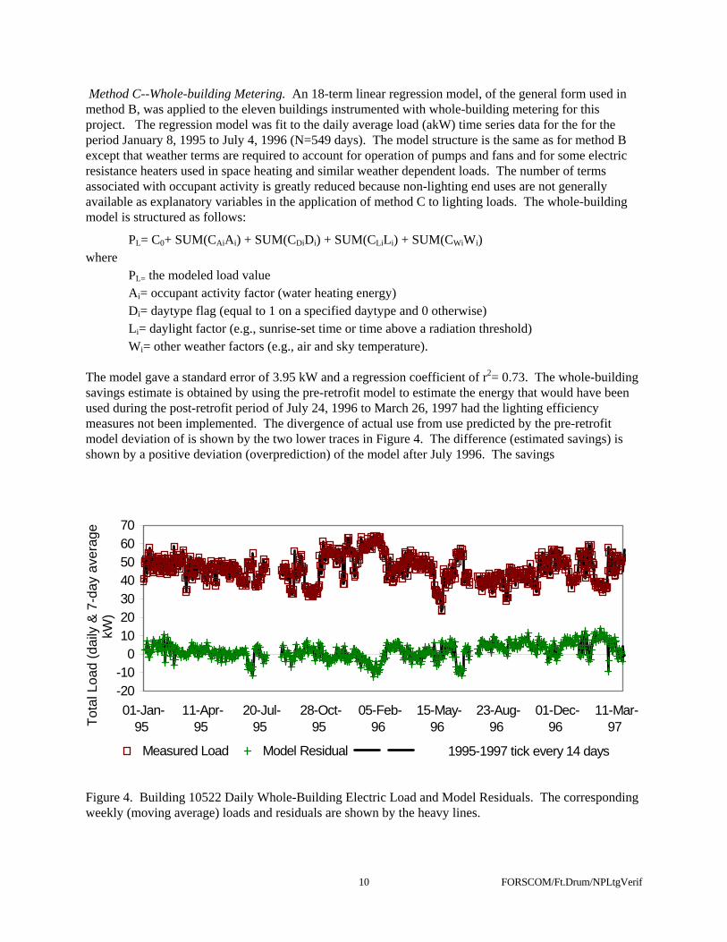
Method C--Whole-building Metering. An 18-term linear regression model, of the general form used in method B, was applied to the eleven buildings instrumented with whole-building metering for this project. The regression model was fit to the daily average load (akW) time series data for the for the period January 8, 1995 to July 4, 1996 (N=549 days). The model structure is the same as for method B except that weather terms are required to account for operation of pumps and fans and for some electric resistance heaters used in space heating and similar weather dependent loads. The number of terms associated with occupant activity is greatly reduced because non-lighting end uses are not generally available as explanatory variables in the application of method C to lighting loads. The whole-building model is structured as follows:

PL= C0+ SUM(CAiAi) + SUM(CDiDi) + SUM(CLiLi) + SUM(CWiWi) where PL= the modeled load value Ai= occupant activity factor (water heating energy) Di= daytype flag (equal to 1 on a specified daytype and 0 otherwise) Li= daylight factor (e.g., sunrise-set time or time above a radiation threshold) Wi= other weather factors (e.g., air and sky temperature). The model gave a standard error of 3.95 kW and a regression coefficient of r2= 0.73. The whole-building savings estimate is obtained by using the pre-retrofit model to estimate the energy that would have been used during the post-retrofit period of July 24, 1996 to March 26, 1997 had the lighting efficiency measures not been implemented. The divergence of actual use from use predicted by the pre-retrofit model deviation of is shown by the two lower traces in Figure 4. The difference (estimated savings) is shown by a positive deviation (overprediction) of the model after July 1996. The savings

-20-10

010203040506070

01-Jan-95

11-Apr-95

20-Jul-95

28-Oct-95

05-Feb-96

15-May-96

23-Aug-96

01-Dec-96

11-Mar-97


Tota

l Loa

d (d

aily

& 7

-day

ave

rage

kW

)

Measured Load Model Residual

Figure 4. Building 10522 Daily Whole-Building Electric Load and Model Residuals. The corresponding weekly (moving average) loads and residuals are shown by the heavy lines.


averaged 4.95 kW from a pre-retrofit average load of 47.4 average kW. Model details are documented in Appendix D. None of the daily load models of the other ten buildings with monitored electric service meters gave regression coefficients of better than 0.6, indicating that little of the daily load variability could be explained by the variables. Method C Extended to Feeder Metering. Nineteen- and twenty-term regression models were fit to the daily average feeder load (akW) time series for the period January 16, 1995 to April 19, 1996. N=394 days after accounting for gaps and inadmissible data. Operational disturbances limited the post-retrofit analysis period to October 2, 1996 through January 16, 1997. Two other major retrofits occurred during the analysis period. New-Post street delamping, which occurred during the pre-retrofit baseline period, is fairly easy to model because the street lamps are controlled by astronomical clocks. Interior lighting was also retrofit in non-prototypical New-Post buildings (division headquarters, clinics, social services and recreational buildings) during September 1996. These actions were not modeled and therefore appear as additional savings. The general form of the feeder level model is: PFDR= C0+ SUM(CAiAi) + SUM(CDiDi) + SUM(CLiLi) + SUM(CWiWi) + SUM(CSiSi) where PFDR= modeled feeder load (akW) Ai= occupant activity factor (based on 10522 water heating) Di= daytype flag3 or adder4 Li= daylight factor (e.g., sunrise-set time or time above a radiation threshold) Wi= weather factor (e.g., air temperature, sky-air temperature difference) Si= street light delamping factor. New-Post street delamping of about 100 kW of connected load (~50 akW) between November 1995 and January 1996 was modeled using an approximate delamping schedule. The value of the street delamping term, S1, for a given day is the product of the "delamping completed" factor and the sunrise-sunset time for that day. The savings range from 5.0 to 8.6% of the average pre-retrofit load. The savings are larger in magnitude than the standard error of the regression from which the savings is estimated in three cases (A2, A3, and B2) and less in one case (B3). The post-retrofit deviations of the model are very close to the models' standard errors except in the case of B3, where it is more than double. These results indicate that the chosen regression model is suitable for feeders A2, A3, and B2, but is not suitable for B3. The plot of the load on B3 supports postulated growth in electrical resistance heater use. Indeed, the load does increase more in cold weather on B3 than it does on the other three feeders, and it appears especially to increase more in response to the cold of late 1996 (the post-retrofit period) than in previous years. The street delamping term was significant for feeders B2 and B3. The connected load reduction from the delamping project implied by the CS1 coefficients in these two feeder models is 30.6 kW. This represents an annual savings of 15 akW or 131 MWh/year, about 30% of the savings expected on all seven New-Post feeders. The implied savings from interior lighting retrofits on the four feeders together is 218 akW, which

3 exactly one of the daytype flags takes a value of 1; all others are 0. 4 any one of the daytype adders may take a value of 1; or all may be 0.


translates to 1915 MWh/year. This includes savings for the non-prototypical building retrofit delivery order as well as the savings for the delivery order of interest. Complete regression modeling results are presented in Appendix E. METHODS AND RESULTS COMPARED All three NEMVP methods have been applied to Building 10522. It is possible to compare Methods A and B for the two common end-use metering cases: pure (all 277-volt interior lighting served by lighting panel LPA) and mixed (subpanels A,B,C,D,G,H,J and K). The results of methods A and C and of methods B and C can only be compared for the aggregate lighting retrofits. Comparison with savings based on operating hours and fixture wattage estimates used in the 1992 IRP study are also of interest. The protocols have been applied to all buildings in the project to obtain aggregate savings estimates. Method A, the extension of method C to feeders, and the original IRP results can be compared at this level. These comparisons are presented in Table 6. TABLE 6. Lighting Savings Comparison by Verification Method Building 10522 Pre-Retrofit

(MWh/year)Post-Retrofit(MWh/year)

Savings(MWh/year)

wrt Pre-Ret Load(%)

IRP 98.0 61.2 36.8 37.6 Method A 154.6 108.4 46.2 27.9 Method B 202.8 170.0 32.8 16.2 Method Ca 415.2 371.7 43.5 10.5

All Barracks Pre-Retrofit Post-Retrofit Savings …as%Pre-Ret IRP 3580 2229 1352 37.8 Method A 4358 2937 1420 32.6 All Buildings Pre-Retrofit Post-Retrofit Savings …as%Pre-Ret IRP 5539 3679 1860 33.6 Method A 6845 4800 2045 29.9 Method C extendeda 29820 28003 1915 b

6.4

Method C adjustedc 1610 5.4aPre- and post-retrofit energy numbers for methods C and C-extended involve all loads whereas the corresponding numbers for other methods include only, or predominately, lighting loads. bThe extended method C savings estimate includes the effect of 9/96 lighting retrofits in New-Post DivHQ, Clinics, Chapels, & Recreation buildings. cMethod C extended has been adjusted by subtracting the 9/96 lighting retrofit savings (estimated).

The main outcome seen in comparing the savings estimates is that method A gave a larger savings estimate than B or C at all aggregation levels. The large discrepancy for method B with respect to methods A and C (which are quite close for Building P-10522) is somewhat misleading. Method B is generally considered the most accurate and there is nothing in its application to Building


10522 that would lead us to believe otherwise. Our conclusion is that both methods A and C over-estimate the savings--but for different reasons. This particular application of method A is unreliable because the hours of operation in soldiers' quarters, which represent the bulk of the connected load, were not sampled. A small additional error may be associated with the nominal, as opposed to measured, values used for pre- and post-retrofit fixture loads. Method C modeling statistics show that the confidence interval is more than wide enough to explain the discrepancy with respect to the method B estimate. The error may be caused by unexplained changes in operation of building electrical equipment, in electrical use tied to occupant activity, or both. Note, incidentally, that the IRP estimate is much closer to the method B estimate than either the method A or method C estimates. The results of applying methods A and C-extended to all buildings in the project tend to confirm the conclusion that the method A estimate is high. In this case, method C-extended includes additional effects of a 9/96 retrofit project. It gives a lower savings estimate even with the benefit of the additional savings. One may be tempted to apply the Building P-10522 ratio of method B/method A savings to correct the method A estimate for all buildings. This cannot be generally recommended without a more definite understanding of the sources of error, and then only for bias, not random, error. For example, the hours of operation measured and assumed for Building P-10522 do not necessarily apply to other buildings of different, or even the same, type. However, the ratio adjusted savings estimate does give a qualitatively useful bracketing point of 1610 MWh/yr for the whole project. The discrepancies are large relative to the savings measured. This is not surprising given the large operating hours variances and burnout variances, the small sampling rates, the large apparent changes in occupant activity and the lack of pre- and post-retrofit connected loads measurements. Because we started well below the point of diminishing returns, there is little doubt that larger sampling rates would have high value, i.e., would improve the savings estimates substantially at low marginal cost. CONCLUSIONS AND RECOMMENDATIONS The objectives of the project were, for the most part, successfully achieved. The uncertainties in savings estimates obtained by the different methods have been documented to serve as an example for FORSCOM sites who may, in future, rely on M&V methods to determine ESCO payments. While it is not possible to reach general conclusions about the relative accuracies of the M&V methods, a strategy that will help any FORSCOM site approach the achievable accuracy limits for a given cost has been developed. In addition, a great deal of practical M&V experience was gained during the project. Many details of the practical lessons learned are compiled in Appendix G. Measured Savings Results. The savings measured by standard and modified protocols were found to differ considerably but generally confirmed the predicted savings. In the case of soldiers' quarters, the method-B results show that actual operating hours were significantly overestimated in the IRP. The savings generated by the lighting retrofit project is estimated to fall between 1610 MWh/yr (adjusted feeder model) and 2045 MWh/yr (stipulated-loads estimate). The savings estimated by the stipulated loads method is unreliable (clearly an overestimate) because of insufficient sample size. Savings estimates obtained by whole-building-level and feeder-level metering also were less reliable than the end-use metering estimates because independent indicators of occupant activity and operational changes were not generally available at the building or higher level. Also, the feeder-level method was confounded by multiple retrofit projects taking place shortly before and after the modeled project on the same feeders. Although a large number of lighting loggers were deployed, the sampling of operational hours for the


stipulated-loads measurement is still far less than optimal. A substantially better SIR could have been achieved for the Fort Drum lighting project by eliminating certain existing lighting applications in which the combination of efficiency improvement, hours of use, and retrofit cost result in low SIR potential. The benefit of identifying these poor prospects prior to retrofit is often sufficient to justify thorough baselining for 6 to 12 months before retrofit work begins. This should be included in the contract if M&V or performance contractor services are to be used. M&V Method Comparison. The choice of a verification method will depend on various factors including the availability and/or ease of obtaining data and desired accuracy of the results. For most simple lighting retrofits, it is likely that method A, B, or a combination of both, will provide the best and most cost-effective results. Table 7, which provides a summary of the characteristics, applications and relative cost efficiency of the different methods, can be used as an aid to method selection. TABLE 7. Method Characteristics Compared Method/Description Advantages Disadvantages Applications Relative Cost A Load-Hours: • Lighting counts • Nameplate or

measured loads • Estimated or

measured operating hours

Provides accurate determination of hours of use, actual in-use fixture load, and fixture count

Requires deployment of many op-time loggers for one to several weeks for each space type; also requires walk-through audit– could be labor intensive

Well suited to lighting retrofits. Works well when occupancy and hours of operation are stable and well defined

Can be least expensive per unit savings if limited monitoring is done. More monitoring and multiple different space types will increase costs.

B End-Use Metering • Measures

energy use by end-use type

Can provide direct clean measurement of energy by end-use before and after retrofit(s)

May not be clean access to lighting circuits. Requires installation of electrical monitoring equipment, data acquisition, and analysis or modeling

Well suited to 277-volt lighting retrofits, motor retrofits, and all other electrical end uses with dedicated circuits

Considered the most expensive per unit savings because of metering installation complexity. Cheaper metering equipment will lower cost.

C Building • Measurement of

whole building energy use

• Modeling using other variables such as weather and occupancy

Easy to monitor building total loads and this type of data may already be available

Usually requires advanced modeling to isolate retrofit effect; ALL time-varying energy-use factors must be monitored. Usually gives only building-aggregate savings

Suited to retrofit projects where ALL variable energy use factors such as weather, activity schedule, and occupancy can be measured--often not the case

Generally lower cost per unit savings than A or B because of simplistic installation. Some metered data may already be available but setting up the model may require different monitoring.

C Feeder • Measurement of

feeder level energy use

• Modeling using variables such as weather, occupancy, and feeder building mix

Monitoring equipment can be economical and easy to install. In conjunction with method C, can verify special retrofits like street lighting.

Usually requires advanced modeling to isolate retrofit effect; ALL time-varying energy-use factors must be measured. Gives only aggregate savings and project phases that overlap complicate modeling.

Is best suited to larger projects where difference in energy use is expected to be large and appears across many buildings. Also attractive for long-term load tracking.

Can be lowest cost per unit savings because of simple, centralized, “set-it-and-forget-it” metering


For lighting retrofits, method A is frequently best when use patterns are repeatable or when the number of fixtures per switch is uniformly large. Method B is generally best when dedicated lighting panels exist. Method C is best when whole-building load profiles are quite repeatable and lighting represents a large fraction of the whole-building load. Careful weather normalization is required. The accuracy of the savings estimates cannot be estimated a priori for any of the methods. Rather, small-scale monitoring may be used in the initial baseline activity to get a preliminary indication of the uncertainties. The full verification plan can then be developed based on the preliminary cost-accuracy trade-offs established. The most important lesson learned from this work is that a close approach to the best accuracy achievable for a given cost can be ensured only by a stepwise procedure where information from early results is used to guide sample size and method selection in later, progressively larger-scale measurement activities. Understanding M&V and its relation to other phases of DSM. The Fort Drum experience has shown that verification protocols and interpretations thereof can give widely varying results. Obtaining sufficiently long and clean (free from load and occupancy changes) pre- and post-retrofit load time-series has been a recurring difficulty. A facility owner should therefore begin preliminary baseline monitoring using a variety of methods at least one year before retrofit activity. Full baseline monitoring should begin at least six months prior to retrofit (including summer periods when cooling interactions are expected and winter when net savings will involve heating interactions). For lighting projects, the monitoring may have to include variables such as daily hours of sunshine, albedo, and sol-air temperature and sky temperature, as well as carefully selected measures of occupant activity such as hot water consumption. Analysis of the preliminary energy-use baseline must be completed far enough in advance of retrofit activity to determine the type(s), extent, and duration of full baseline measurements needed to obtain a given level of verification accuracy. Relatively large samples of equipment operating hours are needed in buildings where occupant activity levels are not simply a function of daytype. This activity has also shown some unexpected attributes of the verification methods. For example, end-use metering (method B) in the barracks showed that hours of operation of lighting in soldiers’ quarters had been overestimated in the IRP. We usually expect to get this kind of information from method A but the problems of access for deploying and retrieving loggers and the large sample needed made method A unattractive. We also found that the confounding effects of overlapping retrofit activities occurring during a data analysis period could be handled successfully by use of models designed to extract separate savings estimates for two projects. Other Recommendations. Fort Drum has been proactive in developing and implementing energy-efficiency projects, yet has not been able to demonstrate savings at the main meter. This is not surprising given the multiple DSM projects, building expansion projects, and a continuous flux of personnel and equipment related to mission objectives. The results of this project show that, even though the load changes attributed to DSM can be tracked better at the building level, it is possible, by applying models that properly account for weather and other effects, to measure them at the feeder or higher level. However, since Fort Drum already has pulse-output meters in place in over half of its floor area and also has two suitable communications networks in place (a building automation network and a water system telemetry network) there is a perfect opportunity to begin tracking energy use at the building level. It would also be relatively easy to extend this concept to basic end-use metering in a sample of the prototypical buildings by monitoring the motor control center and main lighting panels in these buildings. A good baseline for the motor projects identified in the IRP would thus be established and a baseline for “other” (e.g., laundry equipment, refrigerators, computers, vending machines) loads, which have potential future DSM resource, would also be established.


It is a good idea to consider metering improvements when developing a site energy plan. Large sites need a strategic plan for managing energy use. The strategic plan should address the overall goals, planning at all levels, involvement of users and key players, and feedback of energy management actions and results to all stakeholders. A key element of any strategic energy management plan is the tracking of energy use. A good energy tracking system will provide much of the basic data needed for both project design and savings verification. Another key element of the strategic plan is the funding of energy projects. Many energy managers have, in recent years, considered the performance contracting approach (DoD 1991; Executive Order 12902, 1992). Verification methods that measure savings with reasonable accuracy at reasonable cost are a critical part of the performance contracting implementation strategy. The owner, as well as the performance contractor, must understand the strengths and weaknesses of alternative verification methods. And, ideally, the owner should be able check the savings measurements, either with in-house staff or by retaining an independent M&V specialist. One of the main objectives of performance contracting is to shift the risk from the owner, whose decision-making and O&M capability is geared to conventional infrastructure, to a provider with specialized knowledge and capabilities in the analysis, implementation, and operation and maintenance of energy efficient-technologies. Reporting of the energy savings measured and the associated savings uncertainty are crucial to a successful performance contracting arrangement. Few, if any, of the Federal programs that fund energy-efficiency projects at DoD sites have called for a rigorous verification of savings. The funds are typically awarded competitively based on the life-cycle costs of projects as estimated by competing proposers from each DoD site. The omission of verification has led to a culture in which optimistic estimates are necessary for survival. The quality of project designs will not improve as quickly as it would if future design were based on the performance of past designs. This could be corrected by basing future awards on past measured performance. Similar reasoning suggests that measurement and reporting of energy use in new construction should be encouraged or required so that the selection and integration of energy-efficient technologies can be continuously improved. ACKNOWLEDGMENT Dave Carr, Gordon Greene, John Mattingly, George Reynolds, and Steve Rowley of Fort Drum’s Center for Public Works provided invaluable data and other assistance. Lighting loggers were loaned to the project by Niagara Mohawk Power Corporation. PNNL’s Annet Dittmer maintained the polling computer and processed the lighting logger data. REFERENCES Anon. 1996. FORSCOM Executive Summary: Energy Savings Verification at Ft. Drum; see Appendix A Armstrong, P. R., E. E. Richman, D. R. Dixon, and S. Rowley. 1994. "DSM Implementation and Verification at Fort Drum, New York." Proceedings of the 15th World Energy Engineering Conference. Association of Energy Engineers, Atlanta, Georgia. Armstrong, P.R. 1996. Savings Verification at Fort Drum--Interim Report: Detailed Energy Use Baseline, PNNL letter report.


ASHRAE. January 1996. DRAFT ASHRAE Guideline 135P: Measurement of Energy and Demand Savings. American Society of Heating, Refrigeration, and Air-conditioning Engineers, Atlanta, Georgia. BPA. May 1992. Guidelines for Site-Specific Verification. Bonneville Power Administration, Portland, Oregon. Chvala, W. D. Jr., R. R. Wahlstrom, and M. A. Halverson. 1995. Persistence of Energy Savings of Lighting Retrofit Technologies at the Forrestal Building. PNL-10543. Pacific Northwest Laboratory, Richland, Washington. Dixon, D. R., P. R. Armstrong, and K. K. Daellenbach. 1993. Fort Drum Integrated Resource Assessment - Volume 1: Executive Summary. PNL-8424 Vol. 1, Pacific Northwest Laboratory, Richland, Washington. Dixon, D. R., P. R. Armstrong, J. R. Brodrick, K. K. Daellenbach, F. V. DiMassa, J. M. Keller, E. E. Richman, G. P. Sullivan, and R. R. Wahlstrom. 1992a. Fort Drum Integrated Resource Assessment - Volume 2: Baseline Detail. PNL-8424 Vol. 2, Pacific Northwest Laboratory, Richland, Washington. Dixon, D. R., P. R. Armstrong, K. K. Daellenbach, J. E. Dagle, F. V. DiMassa, D. B. Elliott, J. M. Keller, E. E. Richman, S. A. Shankle, G. P. Sullivan, and R. R. Wahlstrom. 1992b. Fort Drum Integrated Resource Assessment - Volume 3: Resource Assessment. PNL-8424 Vol. 3, Pacific Northwest Laboratory, Richland, Washington. DoD Office of the Assistant Secretary of Defense. March 19, 1991. "Implementing Defense Energy Management Goals." Defense Energy Program Policy Memorandum DEPPM-91-2, U.S. Department of Defense, Washington, D.C. Executive Order 12902. March 8, 1994. "Energy Efficiency and Water Conservation at Federal Facilities." Federal Register Vol. 59, No. 047. DOE/FEMP. February 1996. National Energy Measurement and Verification Protocol. U.S. Dept. of Energy NEMVP Subcommittee. Halverson, M.A., J.R. Schmelzer, and G.B. Parker. 1993. Forrestal Building Lighting Retrofit Second Live Test Demonstration (LTD). PNL-8540. Pacific Northwest Laboratory, Richland Washington. Halverson, M.A., J.L. Stoops, J.R. Schmelzer, W.D. Chvala, J.M. Keller, and L. Harris. 1994. Lighting Retrofit Monitoring for the Federal Sector - Strategies and Results at the DOE Forrestal Building. In Proceedings of the American Council for an Energy Efficient Economy 1994 Summer Study on Energy Efficiency in Buildings, Vol.2, pp. 2.137-2.144, August 28 - September 3, 1994, Pacific Grove, California. ACEEE, Washington, D.C. NAESCO. January 1994. Verification Protocols for Commercial, Industrial and Residential Facilities. National Association of Energy Service Companies. NJBRC. April 1993. Measurement Protocol for Commercial, Industrial and Residential Facilities. NJ DSM Rules, New Jersey Board of Regulatory Commissioners.


APPENDIX A. FORSCOM Executive Summary: Energy Savings Verification at Fort Drum (May 1996)

Energy Savings Verification at Fort Drum A pilot program to quantify energy savings at Fort Drum shows that detailed engineering estimates and careful metering and monitoring of actual energy use and energy use factors are critical to accurately verify savings. As Forces Command moves to establish a broad Energy Savings Performance initiative, accurate verification will ensure that Forces Command can offer terms that attract competent ESP contractors but not overpay them because of inaccurate measurements.

The pilot program, conducted by the Pacific Northwest National Laboratory, provided engineering estimates of savings from six energy conservation projects at Fort Drum. PNNL is in the process of measuring the actual savings from each project; three are reported here and additional data is being collected on the other three.

Overall, engineering analyses predicted savings of 230 kilowatts. Energy use measurements indicated a range of savings from 227 kilowatts in some weeks to an increase of 663 kilowatts in others. In general, engineering estimates of savings were higher than the measured savings, as shown in Table 1. More importantly, confounding factors, which were not anticipated when the verification metering was planned and installed, hindered analyses and prevented accurate verification of savings for two of the three projects. More accurate and accessible records about changes in building use, population, and work orders for installation of energy-using equipment might have led to more accurate analyses. Using application-specific verification protocols immediately before and after retrofit activities would have given a much clearer picture of actual savings. Savings information is shown in Table 1.

In early 1995 Fort Drum used FEMP funding to replace incandescent lights with efficient fixtures in entry halls on New-Post. Sixty-eight buildings were retrofitted with 648 compact fluorescent lights. In preliminary studies, project staff estimated that the new lights would reduce the electric load by 39 kilowatts. Measurements indicate the savings were less--about 27 kilowatts. Staff postulate that many of the incandescent lamps were burned out and that the actual load was less than the value in original estimates of potential savings.

A second project, which began in December 1995 and ended in January 1996, retrofitted six buildings at the new airfield with more energy-efficient lighting technologies. The engineering estimate of project savings was 187 megawatt-hours per year. Measurements indicate the project saves only about 56 megawatt-hours per year. Staff speculate that airfield offices are getting only about 25 percent of the use they originally anticipated; leading to a discrepancy between the estimated and measured savings.

A third project removed every other lamp from the New-Post streetlights. De-lamping eliminates 190 kW of connected load, or about 2% of the site’s baseload. A reduction of this magnitude should be very visible at the substation meter. The reduction in electric load was measured at 5 of the 7 feeders that serve 97% of the affected street lights. A constrained regression model of the measured data showed a statistically significant savings of 101 akW or 880 MWh per year.

This Executive Summary is provided by the FORSCOM Energy Branch. For more information, contact Adrian H. Gillespie, Program Manager, (404) 669-7268.

Project Engineering

Analysis Analysis of

Measured Energy Use fixture

quantity load (W) reduction

kW % Use

MWh/yr akW MWh/yr

Replace New-Post Entry Lights with Compact Fluorescent Lights

684 57 39 100 342 27 240

Replace Airfield Lights with T8

202 685 102 730 250

16 32 35 48 64

80 27 187 10 56

De-Lamp New-Post Street Lights

644 295 190 52

867 101 880


APPENDIX B.

SAVINGS IN 10522 BARRACKS/CS&A BASED ON SAMPLED HOURS AND NAMEPLATE LOADS Room

Fixture

Quantity by panel

Fixture Load (W)a

Operating timea

Burned out

Energy Use (kWh/yr)

Area type type Codea LPA SPx Pre- Post- (%) (%) Pre- Post- Change 2nd hall 1x4 rec 2A 10 81.8 61 100 10 6,434 5,331 1,103 2nd exit exit 3A 7 30 1.8 100 50 918 110 808 2nd hall 2x4 rec 2B 4 81.8 61 100 10 2,574 2,133 441 2nd hall 2x4 rec 2E 2 163.6 112 100 10 2,574 1,958 616 2nd tv room 2x4 rec 2D 2 122.7 92 34 2 715 547 168 2nd day room 2x4 rec 2D 5 122.7 92 34 2 1,787 1,367 420 2nd laundry 2x4 rec 2C 2 122.7 86 34 2 715 511 204 2nd mail 2x4 rec 2B 1 81.8 61 5 0 36 27 9 2nd elec/mech 1x4 ind 2P 4 81.8 61 2 0 57 43 15 2nd stair 1x4 wall 2M 1 81.8 61 93 10 598 496 103 2nd vestibule 2x4 rec 2E 4 163.6 112 93 10 4,787 3,641 1,146 2nd janitor ceil mnt 1A 1 75 18 2 0 13 3 10 2nd restroom ceil mnt 1D 1 75 18 34 0 223 53 169 2nd hall ceil can * 5 * * * 10 0 0 0 1st hall 1x4 rec 2A 10 81.8 61 100 10 6,434 5,331 1,103 1st exit exit 3A 13 30 1.8 100 50 1,704 205 1,500 1st hall 2x4 rec 2B 5 81.8 61 100 10 3,217 2,666 551 1st hall 2x4 rec 2E 2 163.6 112 100 10 2,574 1,958 616 1st tv room 2x4 rec 2D 2 122.7 92 34 2 715 547 168 1st day room 2x4 rec 2D 4 122.7 92 34 2 1,429 1,094 336 1st laundry 2x4 rec 2C 2 122.7 86 34 2 715 511 204 1st mail 2x4 rec 2B 1 81.8 61 5 0 36 27 9 1st elec/mech 1x4 ind 2P 4 81.8 61 2 0 57 43 15 1st stair 1x4 wall 2M 3 81.8 61 93 10 1,795 1,487 308 1st janitor ceil mnt 1A 1 75 18 2 0 13 3 10 1st restroom ceil mnt 1D 1 75 18 34 0 223 53 169 1st hall ceil can * 5 * * * 10 0 0 0 HQ hall 2x4 rec 2B 23 81.8 61 54 10 7,992 6,622 1,370 HQ hall 1x4 rec 2Q 2 81.8 61 54 10 695 576 119 HQ hall 2x4 rec 2C 2 122.7 92 54 10 1,042 812 231 HQ hall 2x4 rec 2D 12 122.7 92 54 10 6,254 5,219 1,044 HQ exit exit-dbl 3B 1 30 3.6 100 50 131 31 100 HQ exit exit 3A 13 30 1.8 100 50 1,704 205 1,500 HQ storage 1x4 rec 2Q 46 81.8 61 41 5 12,809 10,055 2,754 HQ storage 1x4 rec 2P 6 81.8 61 41 5 1,671 1,312 359 HQ storage ceil mnt 1D 1 75 18 2 0 13 3 10 HQ classroom 2x4 rec 2D 27 122.7 92 23 2 6,526 4,993 1,533 HQ office 2x4 rec 2C 24 122.7 86 34 5 8,313 6,133 2,180 HQ office 2x4 rec 2D 39 122.7 92 34 5 13,509 9,967 2,847 HQ storage 2x4 rec 2B 3 81.8 61 5 10 97 80 17 HQ restroom 2x4 rec 2B 6 81.8 61 34 0 1,458 1,088 371 HQ restroom 1x4 wall 2M 6 81.8 61 34 0 1,458 1,088 371 HQ elec/mech 1x4 ind 2P 1 81.8 61 2 0 14 11 4 HQ restroom ceil mnt 1G 6 75 18 34 0 1,337 321 1,016 HQ janitor closet porcelin 1A 3 75 18 2 0 39 9 30 HQ catwalk ceil mnt * 11 * * * 0 0 0 Ext exterior wall mnt * 13 * * * 0 0 0 Qtrs restrooms ceil mnt 1D 102 75 18 13 2 8,518 2,086 6,432 Qtrs vanity wall mnt 1E 68 120 26 13 2 13,978 3,090 7,077 Qtrs room 1x4 wall 2M 204 81.8 61 13 2 18,581 14,139 4,442

afixtures not in the project are indicated by * Total LPA (kWh/yr) 122,126 93,046 39,080 bSPx includes SPA,B,C,D and SPG,H,J,K Total SPx (kWh/yr) 19,465 4,542 14,923

Total Annual kWh 141,591 97,588 44,003 Average LPA (kW) 13.97 11.65 3.33

Average SPx (kW) 2.23 0.52 1.71 All project ltg (kW) 16.20 11.17 5.03


APPENDIX C. SAVINGS BY BUILDING TYPE BASED ON SAMPLED HOURS AND NAMEPLATE LOADS

Fixture type 1A 1C 1D 1E 1G 2A 2B 2C 2D 2E 2F 2G 2J 2K 2L 2M 2N 2P 2Q 3A 3B Total Wattage - PRE 75 75 75 120 75 82 82 123 123 164 164 82 82 164 123 82 123 82 82 30 30 avg Wattage -POST 18 18 18 26 18 61 61 86 92 112 122 61 61 112 92 61 86 61 61 1.8 3.6 kW HQ fixt count 58 102 45 0 74 2 609 579 1343 22 210 0 0 0 0 15 0 119 56 173 2 Hr/wk (%) 2 2 2 0 34 2 39 34 34 100 34 0 0 0 0 34 0 36 41 100 100 Burnout(%) 0 0 0 0 0 0 6.3 5 5 10 5 0 0 0 0 0 0 4 5 50 50 Avg Kw - PRE 0 0.2 0 0 1.9 0 18 23 53 3.2 11 0 0 0 0 0.4 0 3.4 1.8 2.6 0 119 Avg Kw -POST 0 0 0 0 0.5 0 14 17 42 2.5 8.7 0 0 0 0 0.3 0 2.6 1.4 0.3 0 90 BRK fixt count 199 3 3851 2496 152 725 967 851 2273 248 4 0 0 0 0 7829 0 615 1595 943 32 Hr/wk (%) 2 2 13 13 34 100 67 34 34 97 34 0 0 0 0 13 0 17 41 100 100 Burnout(%) 0 0 2 2 0 10 5 5 5 10 5 0 0 0 0 2 0 3 5 50 50 Avg Kw - PRE 0.3 0 37 38 3.9 53 50 34 90 35 0.2 0 0 0 0 82 0 8.3 51 14 0.5 497 Avg Kw -POST 0 0 9 8.4 0.9 44 40 25 71 27 0.2 0 0 0 0 62 0 6.4 40 1.7 0.1 335 DH fixt count 2 0 22 0 0 56 90 139 142 3 24 1 0 0 0 1 0 38 377 52 2 Hr/wk (%) 2 0 34 0 0 100 59 59 34 93 34 2 0 0 0 34 0 2 59 100 100 Burnout(%) 0 0 0 0 0 10 1.1 1.1 5 10 5 0 0 0 0 0 0 0 1.1 50 50 Avg Kw - PRE 0 0 0.6 0 0 4.1 4.3 10 5.6 0.4 1.3 0 0 0 0 0 0 0 18 0.8 0 45 Avg Kw -POST 0 0 0.1 0 0 3.4 3.2 7.1 4.4 0.3 1 0 0 0 0 0 0 0 14 0 0 33 VMS fixt count 25 0 0 0 0 0 172 417 9 40 0 320 203 53 240 110 91 876 0 240 37 Hr/wk (%) 2 0 0 0 0 0 54 34 34 100 34 34 34 34 34 34 34 36 0 100 100 Burnout(%) 0 0 0 0 0 0 10 5 5 10 5 5 5 5 5 0 5 4 0 50 50 Avg Kw - PRE 0 0 0 0 0 0 6.8 17 0.4 5.9 0 8.5 5.4 2.8 9.5 3.1 3.6 25 0 3.6 0.6 91 Avg Kw -POST 0 0 0 0 0 0 5.7 12 0.3 4.5 0 6.6 4.2 2 7.5 2.3 2.7 19 0 0.4 0.1 68 VRF fixt count 2 0 0 0 0 0 188 152 0 26 34 45 0 0 0 4 0 347 0 0 0 VRF hours 2 0 0 0 0 0 39 34 0 100 34 34 0 0 0 34 0 36 0 100 100 VRF burnout 0 0 0 0 0 0 6.3 5 0 10 5 5 0 0 0 0 0 4 0 50 50 Avg Kw - PRE 0 0 0 0 0 0 5.6 6 0 3.8 1.8 1.2 0 0 0 0.1 0 9.8 0 0 0 28 Avg Kw -POST 0 0 0 0 0 0 4.5 4.4 0 2.9 1.4 0.9 0 0 0 0 0 7.6 0 0 0 22 Total fixt count 286 105 3918 2496 226 783 2026 2138 3767 339 272 366 203 53 240 7959 91 1995 2028 1408 73 Avg kW - PRE 0.4 0.2 37 38 5.8 58 85 89 149 49 14 9.6 5.4 2.8 9.5 85 3.6 46 71 21 1.1 781 Avg kW -POST 0.1 0 9.2 8.4 1.4 48 67 66 118 37 11 7.6 4.2 2 7.5 65 2.7 36 55 2.5 0.3 548 avgkW decrease 0.3 0.1 28 30 4.4 9.9 18 24 31 12 3.1 2.1 1.2 0.8 2 20 0.9 10 16 19 0.8 233


APPENDIX D REGRESSION MODELS FOR DETERMINING THE RETROFIT SAVINGS IN

P-10555 BARRACKS BY METHODS "B" AND "C" Savings from P-10522 Barracks retrofits have been measured using NEMVP Methods B (end-use metering) and C (building meter). Both methods require a weather- and occupancy-normalization model. The regression modeling results are summarized in Table D.1. The coefficient values, standard errors and t-ratios associated with the independent variables are detailed for each regression model in Tables D.2-D.4. Note that the coefficients of D.2 add to give the coefficients of D.3. The savings also add exactly. However, the standard errors of the coefficients are generally lower for model D.3. Also the regression coefficient (r2) for model D.3 is higher than for either model in D.2. These regression statistics show that the combined savings can be estimated with greater confidence than either of the savings subparts modeled alone. TABLE D.1. Estimated Savings and Regression Statistics from the Four Daily Average Electric Load Models Developed for P-10522 Barracks/CS&A Building.

Modeled Load Whole-Building Lighting + Mixed 277-V Lighting Mixed LPA+DBP+SP* iLPA+SPACGJ iLPA SPACGJ

Savings (akW) 4.9678 3.7487 1.7971 1.9516 Constant 41.731 1.5103 7.9251 -6.415 Standard Error of PL estimate 3.9517 1.8064 1.1134 1.2354 Regression Coefficient (r2) 0.7286 0.8012 0.7661 0.775 Number of Observations 508 508 508 508 Degrees of Freedom 490 486 486 486 Number of Coefficients 18 22 22 22

A 22-term regression model was fit to the daily average load (akW) time series for the period 16 January 1995 to 4 July 1996. Data lost when logger telephone links failed made some days unusable including a weather station gap on 19 February 1996 and barracks logger gaps on July 15, July 29-31, August 1-21 and August 23 in 1995 and February 19, 1996. N=508 days after accounting for these data gaps. The general form of the model is: PL= C0+ SUM(CAiAi) + SUM(CDiDi) + SUM(CLiLi) where Ai= occupant activity factor (water heating, non-lighting circuits., etc.) Di= daytype flag5 or adder6, 5 exactly one of the daytype flags takes a value of 1; all others are 0 6 any one of the daytype adders may take a value of 1; or all may be 0


Li= daylight factor (e.g. sunrise-set time or time above a radiation threshold). The mixed-panel model gave a standard error of 1.24 kW and a regression coefficient of r2=0.78 (where 1.0 is a perfect regression). The lighting panel model gave a standard error of 1.11 kW and a regression coefficient of r2= 0.77. Regression results pertaining to the independent variables are shown in Table D.2. TABLE D.2. Model Coefficients from Regression of P-10522 Interior Lighting Panel and Mixed-Panel Load Data. Subpanel (SPx) loads are further documented in Appendix F. Independent (predictor) Variables Lighting Panel Model Mixed Circuits Model Name Description Units Value StdErr tRatio Value StdErr tRatio C0 Constant akW 7.9251 1.1134 7.1177 -6.415 1.2354 5.1926 CA1 SPE(C1 common area light & plug) akW/kW 0.131 0.7172 0.1826 3.534 0.7958 4.4408 CA2 SPE(C1 vending machines) akW/kW -3.562 0.8067 4.4164 6.4345 0.895 7.1894 CA3 SPE(C1 laundry equipment) akW/kW -0.153 0.0583 2.6211 -0.067 0.0647 1.0351 CA4 SPCR(L1 refrigerators) akW/kW 0.7794 0.6168 1.2636 0.7348 0.6844 1.0736 CA5 SPL(C2 common & utility areas) akW/kW -0.003 0.0686 0.0449 0.5314 0.0762 6.9772 CA6 SPF(Admin plug loads) akW/kW 0.2123 0.0399 5.3253 0.1518 0.0442 3.4321 CA7 DPB(Fan & Pump motors) akW/kW -0.004 0.0218 0.1675 0.1694 0.0242 6.9937 CA8 Service Hot Water(SHW) energy akW/Therm -1.1 12.529 0.0878 -51.36 13.901 3.6945 CA9 B3(SHW) akW/Therm -13.4 11.493 1.1656 -26 12.752 2.0388 CA10 SQRT(SHW) akW/Therm.5 16.044 5.3832 2.9803 34.814 5.9728 5.8289 CA11 B3(SQRT(SHW)) akW/Therm.5 4.0924 4.6348 0.883 11.486 5.1424 2.2335 CA12 F1(SQRT(SHW)) akW/Therm.5 8.1072 1.6788 4.829 8.7548 1.8627 4.7 CD1 Training holiday adder akW -1.285 0.3725 3.4503 -0.071 0.4133 0.1729CD2 Holiday adder akW -2.347 0.2679 8.761 0.4923 0.2973 1.6562 CD3 Christmas adder akW -0.774 0.4063 1.9046 -1.475 0.4508 3.2718 CD4 Friday daytype flag akW -0.758 0.1563 4.8513 0.4092 0.1735 2.3587 CD5 Saturday daytype flag akW -2.688 0.1653 16.257 0.5231 0.1835 2.8515 CD6 Sunday daytype flag akW -2.779 0.1777 15.644 0.4379 0.1971 2.2215 CL1 DL Savings Time flag akW 0.9175 0.1927 4.7614 0.298 0.2138 1.3938 CL2 Albedo akW/(W/m2) -0.016 0.0031 5.1547 0.0066 0.0034 1.9088 CL3 time (fraction) above 9 W/m2 akW -2.476 0.9305 2.6608 -3.171 1.0324 3.0714

Note the importance (high value of the t-statistic or ratio of a coefficient's magnitude to its standard error) of the non-lighting/non-motor loads (a measure of occupant activity) in predicting lighting loads. Also note the importance of the daylight terms showing that occupants use fewer lights or use lights for shorter periods when there is more available daylight. To account for such effects using the stipulated loads method, use of expensive lighting loggers must be increased by an order of magnitude. On the other hand, the t-ratios are rather low for all of the daylight terms, indicating that we cannot place as much confidence in the daylight availability effects as we have for the occupant activity (as measured by other loads) and daytype effects.


The coefficients and outputs of the two models are additive because they are linear, have the same independent variables and same type (daily average kW) of dependent variable. The fit statistics, however, are not additive. Regression of combined interior lighting loads gave a standard error of 1.81, a regression coefficient of r2=0.80 and a savings estimate of 3.75 average kW. Regression results pertaining to the independent variables are shown in Table D.3. TABLE D.3. Combined Model Coefficients from Regression of Aggregate P-10522 Loads for All Panels that Serve Retrofit Lighting. Independent (predictor) Variables Combined Model Name Description Units Value StdErr tRatio C0 Constant akW 1.5103 1.8064 0.8361 CA1 SPE(C1 common area light & plug) akW/kW 3.665 1.1636 3.1496 CA2 SPE(C1 vending machines) akW/kW 2.8721 1.3087 2.1946 CA3 SPE(C1 laundry equipment) akW/kW -0.22 0.0945 2.3235 CA4 SPCR(L1 refrigerators) akW/kW 1.5141 1.0007 1.5131 CA5 SPL(C2 common & utility areas) akW/kW 0.5284 0.1114 4.744 CA6 SPF(Admin plug loads) akW/kW 0.3641 0.0647 5.6296 CA7 DPB(Fan & Pump motors) akW/kW 0.1657 0.0354 4.6798 CA8 Service Hot Water(SHW) energy akW/Therm -52.46 20.327 2.5808 CA9 B3(SHW) akW/Therm -39.39 18.645 2.1127 CA10 SQRT(SHW) akW/Therm.5 50.858 8.7335 5.8234 CA11 B3(SQRT(SHW)) akW/Therm.5 15.578 7.5193 2.0717 CA12 F1(SQRT(SHW)) akW/Therm.5 16.862 2.7237 6.1909 CD1 Training holiday adder akW -1.357 0.6043 2.2449 CD2 Holiday adder akW -1.855 0.4347 4.2674 CD3 Christmas adder akW -2.249 0.6592 3.4116 CD4 Friday daytype flag akW -0.349 0.2537 1.3772 CD5 Saturday daytype flag akW -2.165 0.2682 8.0705 CD6 Sunday daytype flag akW -2.341 0.2882 8.1235 CL1 DL Savings Time flag akW 1.2155 0.3126 3.8881 CL2 Albedo akW/(W/m2) -0.009 0.005 1.8719 CL3 time (fraction) above 9 W/m2 akW -5.647 1.5096 3.7406

Notice that all of the daytype adder and flag coefficients have the expected negative sign, i.e., lighting use is less on Fridays, weekends, and holidays than on regular workdays. The coefficients associated with non-lighting electrical use have the expected positive sign, i.e., non-lighting use is a good predictor of lighting use. One exception is clothes washer and dryer electrical loads. It is possible that higher than normal laundry activity occurs when soldiers return after a day of strenuous outdoor activity during which indoor lighting use is relatively low.


An 18-term linear regression model, of the general form used in method B, was fit to the daily average whole-building load (akW) time series for the period 8 January 1995 to 4 July 1996 (N=549 days). The model structure is the same as for method B except that weather terms are required to account for operation of pumps and fans and some electric resistance heaters used in space heating and similar weather dependent loads. The number of terms associated with occupant activity is greatly reduced because non-lighting end uses are not generally available as explanatory variables in the application of Method-C to lighting loads. The whole-building model is structured as follows: PL= C0+ SUM(CAiAi) + SUM(CDiDi) + SUM(CLiLi) + SUM(CWiWi) where Ai= occupant activity factor (water heating energy) Di= daytype flag (equal to 1 on a specified daytype and 0 otherwise), Li= daylight factor (e.g. sunrise-set time or time above a radiation threshold). Wi= other weather factors (air and sky temperature). The model gave a standard error of 3.95 kW and a regression coefficient of r2= 0.73. Regression results pertaining to the independent variables are shown in Table D.4. TABLE D.4. Model Coefficients from Regression of P-10522 Whole-Building Load Data. Name Description Units Value StdErr TRatio CA1 Constant akW 41.731 3.9517 10.56 CA1 SQRT(SHW) akW/Therm.5 7.509 7.206 10.42 CA2 B3(SQRT(SHW)) akW/Therm.5 1.7103 6.2959 2.7165 CA3 B1(SQRT(SHW)) akW/Therm.5 6.7091 17.876 3.7532 CA4 F1(SQRT(SHW)) akW/Therm.5 1.5032 6.9621 2.1592 CA5 F3(SQRT(SHW)) akW/Therm.5 5.6386 17.161 3.2857 CA6 B1(SHW) akW/Therm -0.718 41.632 1.7243 CA7 F3(SHW) akW/Therm -1.22 41.983 2.9048 CA8 MA41 (41-day movAvg) akW/Therm -2.561 51.399 4.9819 CA8 MA7(SHW)/MA41(SHW) akW -0.056 2.2794 2.4722 CD4 Friday daytype flag akW -0.75 0.5314 1.4111 CD5 Saturday daytype flag akW -1.779 0.5314 3.3485 CD6 Sunday daytype flag akW -0.715 0.525 1.3622 CL1 Sunrise-sunset day fraction akW -18.9 3.2175 5.8752 CL2 Daily solar radiation kW/(W/m2) -0.02 0.0046 4.3621 CW1 Albedo kW/(W/m2) 0.0371 0.0161 2.3044 CW2 Sky-air temperature kW/V -5.308 1.5635 3.3946 CW3 Outdoor temperature kW/V -1.158 0.5346 2.1653


APPENDIX E. REGRESSION MODELS FOR DETERMINING THE RETROFIT SAVINGS ON

FEEDERS BY EXTENSION OF METHOD "C" Nineteen- and twenty-term regression models were fit to the daily average feeder load (akW) time series for the period 16 January 1995 to 19 April 1996. Data lost when logger telephone links failed made 19 February 1996 unusable. Days when non-standard feeder switch positions resulted in non-standard building-feeder mapping, including 22 June - 28 July 1996, 22-24 August 1995, and 25 September - 2 October 1996, were also unusable. A change in switch positions that affected only feeders A3 and B2 eliminated 12-13 September 1995. Thus N=394 days after accounting for the inadmissible data. In the post-retrofit period we observed operational disturbances 17 January and 24-28 February 1997. The post-retrofit analysis period was therefore limited to 2 October 1996 - 16 January 1997. Two other major retrofits occurred during the analysis period. New-Post street delamping, which occurred during the pre-retrofit baseline period, is fairly easy to model because the street lamps are controlled by astronomical clocks. Interior light fixtures in non-prototypical New-Post buildings (division headquarters, clinics, social services and recreational buildings) were retrofit in September 1996. These interior lighting retrofits were not modeled and therefore appear as additional savings. The general form of the model is: PL= C0+ SUM(CAiAi) + SUM(CDiDi) + SUM(CLiLi) + SUM(CWiWi) + SUM(CSiSi) where Ai= occupant activity factor (based on 10522 water heating), Di= daytype flag7 or adder8, Li= daylight factor (e.g. sunrise-set time or time above a radiation threshold), Wi= weather factor (e.g. air temperature, sky-air temperature difference), Si= street light delamping factor. New-Post street lighting was affected by delamping of about 100 kW of connected load (~50 akW) between November 1995 and January 1996. This effect was modeled using an assumed delamping schedule of -6% per workday from 29 October to 10 November 1995, -4%/workday from 10-15 December 1995 and -1%/workday from 7 January to 10 February 1996. The "delamping completed" schedule thus has a value of 1 on and before 29 October 1995 and a value of 0 on and after 11 February 1996. The value of the street delamping term, S1, for a given day is the product of the "delamping completed" factor and the sunrise-sunset time for that day. The regression modeling results are summarized in Table E.1. The coefficient values, standard errors and t-ratios associated with the independent variables are detailed for each regression model in Table E.2.

7 exactly one of the daytype flags takes a value of 1; all others are 0 8 any one of the daytype adders may take a value of 1; or all may be 0


TABLE E.1. Modeled Savings and Associated Regression Parameters and Statistics for Four Daily Feeder Load Models.

Feeder Name: A2 A3 B2 B3 Average load (kW) 1040.185 834.4147 273.7206 1255.847 Constant (kW) 1114.191 884.8467 236.6093 1336.363 Std Err of Y Estimate (kW) 58.73155 56.76305 15.01826 40.54821 R Squared 0.558434 0.679966 0.88215 0.844687 No. of Observations 394 394 539 394 Degrees of Freedom 374 374 520 374 No. of Coefficients 20 20 19 20 savings(akW) 67.80921 72.07996 16.08198 62.5242 rms deviation 59.6882 47.99204 15.07775 84.64314 savings/pre-retrofit load 6.5% 8.6% 5.9% 5.0% TABLE E.2. Model Coefficients from Regression of Feeder Loads.

A2 A3 B2 B3 Name Description Units Value tRatio Value TRatio Value tRatio Value tRatioC0 Constant akW 1114.2 18.97 884.8 15.59 236.6 15.75 1336.4 32.96 CA1 SQRT(SHW) akW/Therm.5 103.33 1.11 173.29 1.92 -7.48 0.35 207.48 3.22 CA2 F3(SHW) akW/Therm 2593.4 3.70 -1002 1.48 60.9 0.41 1191.3 2.46 CA3 SQRT(F3(SHW)) akW/Therm.5 -1099 3.71 672.72 2.35 2.0775 0.03 -502.5 2.46 CA4 MA41(SHW) akW/Therm 259.13 1.21 7.22 0.03 31.42 0.63 340.41 2.30 CA5 MA7(SHW)/MA41(SHW) akW 46.69 2.82 -40.71 2.55 4.74 1.25 27.51 2.41 CD1 Training holiday adder akW -54.38 2.91 -84.23 4.67 -22.97 5.10 -84.64 6.57 CD2 Holiday adder akW -102.1 5.93 -154.4 9.28 -48.98 13.69 -148.1 12.46 CD3 Friday daytype flag akW -40.26 4.20 -40.14 4.33 -6.29 3.05 -44.70 6.75 CD4 Saturday daytype flag akW -144.1 15.76 -155.5 17.59 -52.59 26.36 -189.7 30.04 CD5 Sunday daytype flag akW -126.6 13.64 -149.0 16.61 -62.13 30.86 -176.6 27.57 CD6 Monday daytype flag akW -21.60 2.27 -10.55 1.15 -11.17 5.49 -16.12 2.46 CL1 Daily solar radiation akW/(W/m2) -0.127 1.63 -0.018 0.24 -0.031 2.68 -0.131 2.45 CL2 Sunup day fraction(SSDF) akW -308.3 2.27 -374.2 2.85 -28.6 0.99 -345.8 3.68 CL3 Time(fraction)above 9W/m2 akW 410.9 3.01 165.6 1.26 41.6 1.38 231.3 2.45 CL4 Time(fraction)above 81W/m2 akW -38.6 0.63 -5.8 0.10 -69.0 1.63 CS1 Street delamp factor*SSDF akW -8.4 0.47 -10.8 0.63 11.0 3.93 19.6 1.59 CW1 Sky-air temperature rise akW/(W/m2) -40.80 1.39 17.40 0.61 1.02 0.16 -36.66 1.81 CW2 HDD wrt 12.5°C akW/K -0.233 0.31 1.549 2.15 2.187 4.26 CW3 CDD wrt 9.3°C akW/K -4.886 0.20 8.257 0.35 26.676 1.59 CW4 HDD wrt 30°C akW/K 0.331 1.49 CW5 CDD wrt -9.4°C akW/K 5.362 17.48


The savings range from 5.0 to 8.6% of the average pre-retrofit load. The savings are larger in magnitude than the standard error of the regression from which the savings is estimated in three cases (A2, A3, and B2) and less in one case (B3). The post-retrofit deviations of the model are very close to the models' standard errors except in the case of B3, where it is more than double. These results indicate that the chosen regression model is suitable for feeders A2, A3, and B2, but is not suitable for B3. The plot of the load on B3 supports the explanation, given by the site utility and energy managers, which is growth in electrical resistance heater use for engine block heaters and supplemental space heating. Indeed, the load does increase more in cold weather on B3 than it does on the other three feeders and it appears especially to increase more in response to the cold of late 1996 (the post-retrofit period) than in previous years. Note that the street delamping term is significant (high value of the t-statistic or ratio of a coefficient's magnitude to its standard error) for feeders B2 and B3. The connected load reduction from the delamping project implied by the CS1 coefficients in these two feeder models is 30.6 kW. This represents an annual savings of 15 akW or 131 MWh/year. An additional daylight-availability term, time-fraction above 81 W/m2, is significant in two of the feeder models. Each of the occupant activity terms is significant in at least two of the four models and most are significant in all models. The daytype coefficients all have the expected sign and relative magnitudes in all four models. The implied savings for the four feeders together is 207 akW, which translates to 1820 MWh/year. This includes savings for the non-prototypical building retrofit delivery order as well as the savings for the delivery order of interest.


APPENDIX F. END-USE METERING IN P-10522 BARRACKS/CS&A BUILDING End-use metering equipment was installed in Building P-10522 in May 1994. This is a 2-story building with two barracks wings (30,263 ft2) and an administrative wing (13,623 ft2). The two-story barracks section has a nominal occupancy of 136 residents. The first- and second-floor plans are identical with 9 left-wing and 8 right-wing modules per floor. Each module, consisting of a bathroom and two dorm rooms, accommodates four soldiers. There are 10 common-area rooms per floor including one each for mail, storage, TV/game room, dayroom, vending machines, laundry, toilet, janitorial, electrical, and mechanical equipment rooms, which are arranged around a central foyer. The right and left corridors, set at right angles, extend from the foyer to the soldiers' quarters in each barracks wing. The company administrative and supply (CS&A) wing contains offices, communications, meeting rooms, and storage rooms. Fans and pumps are powered from the same motor control panel as the barracks fans and pumps and 277-volt lighting shares LPA with barracks circuits. Other CS&A end uses receive their power from two panels that are dedicated to CS&A wing circuits. The connected loads, derived from as-built drawings, are listed in Table F.1 by end use. Complete separation of end uses was not possible (as it rarely is) because of mixed circuits and the existence of subpanels at more than one location. The need to contain verification costs prompted some end-use sampling, even in cases where complete coverage was technically feasible. Thus, while the table shows that end uses have been disaggregated at the subpanel level for several important end-use categories, such disaggregation was typically implemented in only one of several similar load distribution panels. Note, for example, that the connected load mix is nearly identical on subpanels A/B, C/D, G/H, and J/K. Separate sampling of refrigerator loads was therefore undertaken only on subpanel A, while subpanels C, G and J were monitored as a single load. The load mixes on panels E and L are also nearly identical; laundry and vending machine loads were therefore monitored only on panel E. With this scheme, separate accounting of end-use loads is effectively accomplished for 96% of the connected load using two data loggers with ten 3-phase and two 1-phase channels between them.


TABLE F.1. Connected Loads (W) by Subpanel (across) and Circuit (down) *wing R1 L1 C1 R2 L2 C2 Adm Adm all "pure" Major small panel SPA SPC SPE SPG SPJ SPL SPF LPA DPB distinct Load misc.

brkr Amps 45 70 70 45 70 45 45 125 150loads Groups loads

refrig 6300 9000 6300 9000 30600 plug 19400 27560 19400 27560 93920

plug & ltg 13650 19500 13650 19500 66300 fire alarm 400 400

pump 200 200 400

W&D 22800 17100 39900 vending 6000 6000 12000

rec can ltg 660 660 1320fan,pmp,UH 2650 2960 5610

plug 3840 3840 7680 water clr 600 600 1200

CATV system 4200 4200 8400exterior ltg 700 700

plug 26460 26460 fluoresc. ltg 1200 1200

plug & ltg 1740 1740 humidifier 3600 3600fan & pmp 5760 5760

class TV 4200 4200

incand. ltg 300 300277v Brk 31800 31800

277v Adm 23150 23150 ext & site ltg 4882 4882

Brk fan&pmp 59945 59945 Adm fan&pmp 46010 46010

Total 39750 56060 41450 39550 56260 35360 42960 60132105955 142332 314625 20520*Rn=right barracks wing, Ln=left barracks wing, Cn=barracks core, Adm=supply & admin wing, n=1 for 1st floor, n=2 for 2nd floor


APPENDIX G M&V LESSONS LEARNED We encountered a number of problems and learned some important lessons in the Fort Drum verification effort. Our observations specific to each method and to verification in general are summarized below. Method A: - Increased sample size and duration are needed to obtain good hours-of-operation data. A minimum of

five lighting circuits should be monitored for spaces that are occupied on a very routine schedule (e.g. dining hall service lines) and it may be necessary to monitor 20 or more circuits when space usage does not follow a known schedule (e.g. soldiers' quarters). Multiple samples are needed even for circuits switched at the breaker panel, which are often erroneously assumed to operate 24 hours/day.

- Connected loads should be based on measured, rather than ANSI or nameplate, data. A relatively small sample of pre- and post-retrofit loads is needed for each fixture type. Sample size is a somewhat logarithmic function of the total number of fixtures of a type. For example, 10 of 200 fixtures of a given type might be sampled in a small project and perhaps 50 of 10,000 in a large project. Accurate volt, amp, and power factor records are needed of each sampled pre- and post-retrofit fixture.

- A detailed verification plan, including the responsibilities of contract administrators and job monitors, must be established as soon after project inception as possible. Elements of the plan should include pre-retrofit burnout counts and operating hours measurements as well as pre- and post-retrofit fixture counts and connected load measurements.

- Method A is probably not the lowest cost way to measure savings in barracks. End-use metering (method B) at a few circuits in 2 or 3 barracks would probably get a much better measure of savings for soldiers' quarters than method A even with a very large lighting logger sample.

Method B: - Larger samples (e.g. monitor multiple buildings) can be justified in a project the size of Fort Drum's

New-Post prototypical building lighting retrofit. - Method B is traditionally considered the most expensive; to obtain larger samples, therefore, the

industry needs lower-cost monitoring systems (hardware, software, method of installation and operation). Fort Drum and other FORSCOM sites need to periodically re-evaluate the costs and capabilities of available tools.

- When there are, as at Fort Drum, multiple buildings representing each of several prototypes, the prudent energy manager will perform end-use metering on at least one of each of the prototypes.

Method C: - Better models are needed. Regression models with physically meaningful variables and parameters

are preferred. Non-linear models in which the parameters are grouped into direct, interactive and non-interactive--with a meta-parameter for each group accounting for ALL of the change between the pre- and post-retrofit period--are probably the most robust and widely applicable across sites and building types. Better software analysis environments are needed to use these models effectively. The multiple linear regression capability of standard current spreadsheet software is not adequate for the intensive verification analysis demanded by large projects such as Fort Drum's.

- Great care is needed in selecting and monitoring the independent (explanatory) variables. It is


important to observe as many potentially significant independent variables as possible, especially measures of general occupant activity, end-use-specific activity, and per capita load growth. The measurement of albedo and domestic water heating, which were included in this spirit, turned out to be crucial to the lighting load models: albedo as a predictor of need to supplement natural lighting, and domestic water heating as a surrogate for general occupant activity.

- Better indicators of occupant activity are needed. Daily domestic hot- and cold-water flows, as well as water heating energy, should be measured.

- Pulse recorders that are much smaller and lower cost than those used in the Fort Drum work are now available. This makes monitoring of all permanent buildings that do not get some other form of automated meter reading (telemetry, EMCS or other) network very feasible.

Method C Extended (Feeder Metering): - The owner must be committed to metering a subset of buildings. All new buildings and

additions, and at least one of each prevalent building type on each feeder, should be metered to account for the effects of new buildings and buildings with load growth.

All Methods: - Start complete monitoring at least six months in advance and review the need for additional high- and

low-level monitoring after 3, 6 and 9 months of data have been analyzed; - Find better ways to track and account for occupancy and occupant/operator behavior, - Reduce costs by using qualified M&V contractors, including the retrofit contractor when

appropriate, for selected tasks, - When using the current NEMVP protocols, always try to use the most rigorous method(s) and

the most rigorous options offered within any given method, - When using multiple methods, plan for at least one subsample of each retrofit class (lighting,

motors, etc.) that is covered by all the methods; compare and diagnose the baseline energy use and adjust sampling rates and the method mix well before retrofit activity begins.

Diagnosing Fort Drum M&V problems. A number of problems appeared specific to the Fort Drum verification measurements and analysis. A modest effort would likely discover most of the root causes of the discrepancies and excessive confidence intervals (statistical uncertainty) noted in this report. The recommended diagnostic tests and metering include: - Connected load measurements of all pre- and post-retrofit fixture types, - A check of 10522 connected lighting loads by panel, - A check of 10500 building-level meter calibrations, - Addition of end-use channels to disaggregate Building 10522 LPA loads into office, briefing room,

utility room, CS&A hall, barracks hall, and living quarters loads, - Connection of the existing 10522 DHW flow meter to one of the existing logger pulse-input channels, - Addition of DHW consumption meters at barracks and dining halls, and - Analysis of 10500-area buildings after additional post-retrofit records have been collected.

summary motivation. objectives. measured savings.web.mit.edu/parmstr/www/pubs/npi-ltg12.pdf ·...

Documents