1

American Institute of Aeronautics and Astronautics

Summary of Data from the Fifth AIAA

CFD Drag Prediction Workshop

David W. Levy1 and Kelly R. Laflin

2

Cessna Aircraft Company, Wichita, KS 67215, USA

Edward N. Tinoco3, John C. Vassberg

4, Mori Mani

5, and Ben Rider

6

The Boeing Company, Seattle, WA, 98124, Huntington Beach, CA 92647, St. Louis, MO, 63301, USA

Chris Rumsey7, Richard A. Wahls

8 and Joseph H. Morrison

9

NASA Langley Research Center, Hampton, VA 23681, USA

Olaf P. Brodersen10

and Simone Crippa10

DLR Institute of Aerodynamics and Flow Technology, 38108 Braunschweig, Germany

Dimitri J. Mavriplis11

University of Wyoming, Laramie, WY 82071, USA

and

Mitsuhiro Murayama10

Japan Aerospace Exploration Agency, Chofu, Tokyo 182-8522, Japan

Results from the Fifth AIAA CFD Drag Prediction Workshop (DPW-V) are presented.

As with past workshops, numerical calculations are performed using industry-relevant

geometry, methodology, and test cases. This workshop focused on force/moment predictions

for the NASA Common Research Model wing-body configuration, including a grid

refinement study and an optional buffet study. The grid refinement study used a common

grid sequence derived from a multiblock topology structured grid. Six levels of refinement

were created resulting in grids ranging from 0.64x106 to 138x10

6 hexahedra – a much larger

range than is typically seen. The grids were then transformed into structured overset and

hexahedral, prismatic, tetrahedral, and hybrid unstructured formats all using the same

basic cloud of points. This unique collection of grids was designed to isolate the effects of

grid type and solution algorithm by using identical point distributions. This study showed

reduced scatter and standard deviation from previous workshops. The second test case

studied buffet onset at M=0.85 using the Medium grid (5.1x106 nodes) from the above

described sequence. The prescribed alpha sweep used finely spaced intervals through the

zone where wing separation was expected to begin. Some solutions exhibited a large side of

body separation bubble that was not observed in the wind tunnel results. An optional third

case used three sets of geometry, grids, and conditions from the Turbulence Model Resource

website prepared by the Turbulence Model Benchmarking Working Group. These simple

cases were intended to help identify potential differences in turbulence model

implementation. Although a few outliers and issues affecting consistency were identified, the

majority of participants produced consistent results.

1 Principal Engineer, AIAA Associate Fellow 2 Engineer Specialist, Sr., AIAA Associate Fellow 3 Boeing Technical Fellow (Retired), AIAA Associate Fellow 4 Boeing Technical Fellow, AIAA Fellow 5 Boeing Sr. Technical Fellow, AIAA Associate Fellow 6 Sr. Engineer, AIAA Member 7 Senior Research Scientist, AIAA Fellow 8 Assistant Head, Configuration Aerodynamics Branch, AIAA Associate Fellow 9 Head, Computational AeroSciences Branch, AIAA Associate Fellow 10 Research Engineer, AIAA Member 11 Professor Mechanical Engineering, AIAA Associate Fellow

https://ntrs.nasa.gov/search.jsp?R=20130003313 2018-05-27T14:27:34+00:00Z

2

American Institute of Aeronautics and Astronautics

I. Nomenclature

AR Wing Aspect Ratio

b Wing Span

BL Butt Line Coordinate

CD Drag Coefficient (CD_TOT)

CDP Idealized Profile Drag = CD −CL2/AR

CDpr Pressure Drag Coefficient (CD_PR)

CDsf Skin-Friction Drag Coefficient (CD_SF)

CL Lift Coefficient

CM Pitching Moment Coefficient (CM_TOT)

CP Pressure Coefficient = (P−P∞)/q∞

Cref Wing Reference Chord ~ MAC

Cf Local Coefficient of Skin Friction

FS Fuselage Station Coordinate

LE Wing Leading Edge

MAC Mean Aerodynamic Chord

N Number of unknowns (GRIDSIZE)

RANS Reynolds-Averaged Navier-Stokes

RE Reynolds Number

Sref Reference Area

SOB Side-of-Body

TE Wing Trailing Edge

WL Water Line Coordinate

y+ Normalized Wall Distance

Angle of Attack (ALPHA)

Fraction of Wing Semi-Span

II. Introduction

The AIAA CFD Drag Prediction Workshop (DPW) Series was initiated by a working group of members from

the Applied Aerodynamics Technical Committee of the American Institute of Aeronautics and Astronautics. The

primary goal of the workshop series is to assess the state-of-the-art of modern computational fluid dynamics

methods using geometries and conditions relevant to commercial aircraft. From the onset, the DPW organizing

committee has adhered to a primary set of guidelines and objectives for the DPW series:

Assess state-of-the-art Computational Fluid Dynamics (CFD) methods as practical aerodynamic tools for

the prediction of forces and moments on industry-relevant geometries, with a focus on absolute drag.

Provide an impartial international forum for evaluating the effectiveness of CFD Navier-Stokes solvers.

Promote balanced participation across academia, government labs, and industry.

Use common public-domain subject geometries, simple enough to permit high-fidelity computations.

Provide baseline grids to encourage participation and help reduce variability of CFD results.

Openly discuss and identify areas needing additional research and development.

Conduct rigorous statistical analyses of CFD results to establish confidence levels in predictions.

Schedule open-forum sessions to further engage interaction among all interested parties.

Maintain a public-domain accessible database of geometries, grids, and results.

Document workshop findings; disseminate this information through publications and presentations.

Four previous workshops have been held prior to the present study, all held in conjunction with the AIAA

Applied Aerodynamics Conference for that year:

Year Location Configuration Case Descriptions

2001 Anaheim, CA DLR-F4 Wing-Body Single Point Grid Refinement Study

Drag Polar

Drag Rise Curves at Constant CL*

2003 Orlando, FL DLR-F6 Wing-Body

Wing-Body-Nacelle

Single Point Grid Refinement Study

Drag Polar

Boundary Layer Trip Study*

Drag Rise Curves at Constant CL*

2006 San Francisco, CA DLR-F6 Wing-Body with

and without FX2B fairing;

W1/W2 Wing Alone

Single Point Grid Refinement Study

Drag Polar

Grid Convergence Study

Drag Polar

2009 San Antonio, TX Common Research Model

Wing-Body and Wing-Body-Tail

Grid Convergence Study

Downwash Study

Mach Sweep Study*

Reynolds Number Study*

*Optional Cases

3

American Institute of Aeronautics and Astronautics

While there have been some variations, the workshops have typically used subjects based on commercial

transport wing-body configurations - a consensus of the organizing committee based on a reasonable compromise

between simplicity and industry relevance. The vast majority of the participants submit results generated with

Reynolds Averaged Navier-Stokes (RANS) codes, although the organizing committee does not restrict the

methodology.

The first Drag Prediction Workshop1 used the DLR-F4 geometry for the above reasons and due to the

availability of publically released geometry and wind tunnel results2. The focus of the workshop was to compare

absolute drag predictions, including the variation due to grid type and turbulence model type. The results were also

compared directly to the available wind tunnel data. The workshop committee provided a standard set of multi-

block structured, overset, and unstructured grids for the DLR-F4 geometry to encourage participation in the

workshop and reduce variability in the CFD results. However, participants were also encouraged to construct their

own grids using their best practices so that learned knowledge concerning grid generation and drag prediction might

be shared among workshop attendees. The test cases were chosen to reflect the interests of industry and included a

fixed-CL single point solution, drag polar, and constant-CL drag rise data sets. To help encourage wide participation,

a formal paper documenting results was not required at the workshop. Eighteen participants submitted results, using

14 different CFD codes; many submitted multiple sets of data exercising different options in their codes, e.g.,

turbulence models and/or different grids. A summary of these results was documented by the DPW-I organizing

committee3. Because of strong participation, DPW-I successfully amassed a CFD data set suitable for statistical

analysis4. However, the results of that analysis were rather disappointing, showing a 270-drag-count spread in the

fixed-CL data, with a 100:1 confidence interval of more than ±50 drag counts.

Despite the somewhat disappointing results, the consensus of the participants and organizers was that DPW-I

was a definitive success. First and foremost it was initiated as a “grass roots” effort by CFD developers, researchers,

and practitioners to focus on a common problem of interest to the aerospace industry. There was open and honest

exchange of common practices and issues which identified areas for further research and scrutiny. The workshop

framework was tested successfully on high fidelity 3D RANS methods using a common geometry, grids, and test

cases. Finally, it reminded the CFD community that CFD is not a fully mature discipline.

The interest generated from the workshop was continued and resulted in several individual efforts documenting

results more formally5-8

, presented at a special session of the 2002 AIAA Aerospace Sciences Meeting and Exhibit

in Reno, NV. The interest generated by DPW-I naturally led to the planning and organization of the 2nd AIAA

Drag Prediction Workshop, DPW-II. The DPW-II organizing committee, recognizing the success of DPW-I,

maintained the format and objectives for DPW-II.

The second workshop9 used the DLR-F6 as the subject geometry in both wing-body (WB, similar to DLF-F4)

and wing-body-nacelle-pylon (WBNP) form. The DPW-II organizing committee worked with DLR and ONERA to

make pertinent experimental data available to the public domain. One specific objective of DPW-II was the

prediction of the incremental drag associated with nacelle/pylon installation. The F6 geometry contained pockets of

flow separation more severe than the F4; occurring predominantly at the wing/body and wing/pylon juncture

regions. The results from the workshop were documented with a summary paper,10

a statistical analysis,11

an invited

reflections paper12

on the workshop series, and numerous participant papers13-21

in two special sessions of the 2004

AIAA Aerospace Sciences Meeting in Reno, NV. A conclusion of DPW-II was that the separated flow regions

made it difficult to draw meaningful conclusions with respect to grid convergence and drag prediction. During the

follow-up open-forum discussions, the CFD community voiced the desire for the organizing committee to include in

the third workshop: a) Blind Test Cases, and b) Simpler Geometries. The request for blind test cases is motivated by

an earnest attempt to better establish a measure of the CFD community’s capability to predict absolute drag, rather

than match it after-the-fact. The request for simpler geometries allows more extensive research in studies of

asymptotic grid convergence.

The third workshop22

retained the DLR-F6 WB from DPW-II as a baseline configuration to provide a bridge to

the previous workshop. However, to test the hypothesis that the grid-convergence issues of DPW-II were the direct

result of the large pockets of flow separation, a new wing-body fairing was designed to eliminate the side-of-body

separation. Details of the FX2B fairing design are documented by Vassberg23

. In addition, to help reduce the wing

upper-surface trailing-edge flow separation, a higher Reynolds number was introduced for the WB test cases. These

changes in both geometry and flow condition also provided the DPW-III participants a blind test since no test data

would be available prior to the workshop. Furthermore, two wing-alone geometries were created to provide

workshop participants with simpler configurations on which more extensive grid-convergence studies could be

conducted; these wings were designed to exhibit no appreciable separation at their design conditions. The DPW-III

was heavily documented with summary papers24,25

, a statistical analysis paper26

, participant papers27-30

, and a special

section of the AIAA Journal of Aircraft, edited by Vassberg31–36

. After three workshops, the organizing committee

4

American Institute of Aeronautics and Astronautics

recognized that a recurring theme of the workshop series was related to grid quality and resolution – see Mavriplis et

al.37

.

For the fourth workshop38

a completely new geometry was developed, called the Common Research Model

(CRM). The CRM was developed by NASA’s Subsonic Fixed Wing (SFW) Aerodynamics Technical Working

Group (TWG), in collaboration with the DPW Organizing Committee. This wing-body-horizontal (with and

without nacelle-pylons) configuration is representative of a contemporary high-performance transonic transport. A

detailed description of its development is given by Vassberg et al.39

.

One aspect of DPW-IV different from the first three workshops was in the timing of the availability of wind-

tunnel test data on the subject geometries. In DPW-IV, the workshop was held before any experimental data were

collected and is a set of blind tests. Another advantageous outcome of this collaborative endeavor is that the CRM

has been tested in two facilities thus far, and the data from these tests is publicly available. The National Transonic

Facility (NTF) at NASA Langley tested the CRM during Jan-Feb 2010, and then it was evaluated at the Ames 11-ft

wind-tunnel during Mar-Apr 2010. Data from the NTF and Ames tests have been released to the public domain by

Rivers and Dittberner40-42

.

Due to past observations of grid dependence on the solutions, a greater emphasis was placed on establishing

meshing guidelines for the generation of baseline grid families. With these guidelines in place, grids were requested

from several organizations for structured multiblock, overset, and unstructured types. Each grid family was required

to include a Coarse (C), Medium (M), and Fine (F) grid; adding an optional Extra-Fine (X) grid was also

encouraged. Target sizes for these grids were 3.5, 10, 35, and 100 million unknowns, respectively. The Medium

mesh was intended to be representative of current engineering applications of CFD being used to estimate absolute

drag levels on similar configurations. A total of 74 meshes of 18 families were provided and made available to

participants for use.

The fourth workshop requested grid convergence and Mach sweep computations as in the previous workshops,

plus downwash and Reynolds Number studies. Data were submitted from 19 organizations totaling 29 individual

datasets. For the grid refinement study, a Richardson Extrapolation methodology was employed to estimate a

continuum value for the total drag coefficient. The range for the total drag coefficient spanned 152 counts, which is

a definite improvement over DPW-I. (Excluding a single outlier, the scatter band reduces dramatically to 41

counts.) While this improvement is quite significant, the confidence level is not down to a low enough level to

compete with experimental methods. Documentation for these results can be found in summary papers43-44

and in

individual contributing papers45-58

from two special sessions held at the 28th

Applied Aerodynamics Conference in

June 2010.

Despite the emphasis placed on grid generation with the intent of reducing the associated errors, the variation in

the results was still disappointing. For the fifth workshop59

, a new approach was taken with the intent of reducing

grid-related errors even further. As with the fourth workshop, the NASA Common Research Model wing body

configuration was used for the geometry. For the grids, a unified baseline60

family of Multiblock Structured meshes

were developed with six different levels ranging in size from 136x106 (Superfine) to 0.64x10

6 (Tiny). Each

successive coarse level was derived directly from the finest mesh. Only five blocks were used. Once the cloud of

points was defined for this series of grids, then Overset and Unstructured grids were derived. The unstructured grids

were defined in Hexahedral, and Prismatic elements, plus a hybrid grid with Prismatic boundary layer and

Tetrahedral field elements was defined.

The test cases included a grid refinement study using the common grids or user-supplied custom grids if desired.

The second case focused on buffet prediction, with a finely spaced alpha sweep spanning the range where flow

separation on the wing was observed in the wind tunnel data and the results in DPW-IV. This is a change from

previous workshops, where angle-of-attack sweeps from 0 to 4° were calculated for the purpose of determining

trimmed drag polars. The high-speed lines development is less than 25% of the total Aerodynamics related airplane

development effort. Significant effort must also be paid to Loads and Stability and Control concerns. Many of these

high-speed flight concerns occur at the edges of the flight envelope, which are characterized by large regions of

separated flows. For the Fifth Drag Prediction Workshop the buffet study has been included to assess CFD

prediction in this regime. The optional third test case used geometries, grids, and conditions from the Turbulence

Model Resource website61

prepared by the Turbulence Model Benchmarking Working Group. Three cases were

selected: 1) 2D Zero Pressure Gradient Flat Plate, 2) 2D Bump-in-channel, and 3) 2D NACA 0012 Airfoil. These

test cases were designed to discriminate between turbulence model implementations through rigorous grid

convergence studies.

This paper presents an overview of the geometry and grid definitions used for the fifth Drag Prediction

Workshop. The participant data for the Case 1 grid refinement study are analyzed, including Force/Moment

predictions, wing pressure distributions, and flow separation at the wing/body trailing edge juncture. A Richardson

5

American Institute of Aeronautics and Astronautics

Extrapolation is performed to estimate the continuum force levels. Comparisons are made to force, moment, and

pressure data from the NTF and Ames wind tunnel tests. Analysis of the Case 2 buffet study is presented, including

force/moment and pressure predictions with comparisons to wind tunnel data. Flow separation predictions at the

wing/body trailing edge juncture and wing trailing edge are shown. Detailed grid convergence studies for drag and

skin friction coefficient for the Case 3 Turbulence Modeling results are also discussed.

II. Geometry Description

The subject geometry for DPW-V Cases 1 and 2 is the Common Research Model39

(CRM) developed jointly by

NASA’s Subsonic Fixed Wing (SFW) Aerodynamics Technical Working Group (TWG) and the DPW Organizing

Committee. The CRM is representative of a modern transonic commercial transport airplane, and was designed in

the full configuration with a low wing, body, horizontal tail, and engine nacelles mounted below the wing. For this

workshop, only the wing-body configuration was used. A rendering of the geometry is shown in Figure 1, along

with a photo of the wind tunnel model installed in the NASA Ames 11ft Transonic Wind Tunnel (with horizontal

tail). The CRM was also the subject geometry for DPW-IV.

The wing was designed for a nominal conditions of Mach=0.85, CL=0.50, and Reynolds Number 40x106 based

on cref. Pertinent geometric parameters are listed in Table 1. The wing is a supercritical design, and the Boeing

Company took the lead on the aerodynamic design. Certain features were designed in to the wing profile for the

purposes of research and development. The upper-surface pressure recovery over the outboard wing is intentionally

made aggressively adverse over the last 10-15% local chord to promote separation of the upper-surface boundary

layer in close proximity to the wing trailing edge (TE) at lift conditions slightly above the design point. The strong

adverse pressure gradient will likely amplify the differences in various turbulence models that may be employed by

DPW participants. The span loading was designed to be very nearly elliptical as compared to a more practical

design which will find a compromise distribution due to structural constraints. This feature is included to provide a

challenge for possible future workshops on aerodynamic shape optimization.

III. Gridding Guidelines and Description of Common Grids

As mentioned above, a common theme and discussion topic in the DPW series is the effect of the computational

grid on the results. A substantial effort was made in DPW-IV to address this, yet there was still significant variation

in the results among the different grid types. The Organizing Committee recognized that a relatively simple

Multiblock Structured (MB) grid could be created for the CRM wing-body geometry that conformed to the desired

gridding guidelines. These gridding guidelines have been developed over the course of the DPW series and are

listed in Table 2. The grid topology for the MB grid is shown in Figure 2.

The finest grid (L6) was generated first and is sized to extend well into the asymptotic range of grid

convergence, while the coarsest grid (L1) would still be “multigrid friendly” for up to 3 levels. The next coarser

level (L5) was obtained by replacing every three cells in each of the I, J, & K directions with two cells. The L4 grid

was created from L6 by removing every other point in each of the (I, J, & K) directions, and L3 by doing the same

starting from the L5 grid. The process is repeated with the L4 and L3 grids to complete the sequence at L2 and L1.

By interleaving the even and odd levels a complete family of six grids is constructed. See Vassberg60

for detailed

information.

Once the MB series was developed, then a set of unified grids for other types were derived. The Overset series

was created by extending each block using data from neighboring blocks to define four patch grids to bridge each

block. The patch grids overlap each block by three cells as shown in Figure 3, and are point matched to minimize

interpolation errors. One issue was found on the K=1 plane for the mid-body block, where the J line had mixed

symmetry plane and block boundary conditions. This issue caused difficulty for some participants.

Three types of unstructured grids were created from the MB grids: Hexahedral, Prismatic, and Hybrid

Tetrahedral (Prismatic in the boundary layer and Tetrahedral in the field). The hexahedral format preserves the

individual cell structure of MB grids, but converts the file into finite element form with no IJK structure.

Subdivision of hexahedral elements into prismatic and tetrahedral elements follows the sequence shown in Figure

4a. Each hex cell subdivides into 2 prism cells, and then each prism is split into 3 tetrahedra. A usable fully

tetrahedral grid could not be created due to issues at the trailing edge of the wing. Groups of cells inside the

boundary layer were distorted such that when subdivided into a negative volume would result (Figure 4b). The

prisms did not have this issue, so only the hybrid grids were created. Negative volumes were also encountered for

the prism subdivision on the Super Fine grid, so only Hex meshes are available at that level.

A summary comparison of the grid sizes for all levels and types is listed in Table 3. Note that suitable grid

refinement sequences are available for unstructured cell- or node-based schemes.

6

American Institute of Aeronautics and Astronautics

IV. Test Case Descriptions

It is recognized that many of the DPW participants are derived from industry and may have limited time and

resources to devote to this type of study. The test case specifications, as with the grid definitions, are set to

encourage participation by restricting the number of cases to a manageable number while also providing a challenge

to test the state of the art in CFD prediction capabilities. The DPW-V test cases contain a set of required and

optional conditions:

Case 1 – NASA Common Research Model (CRM) Wing-Body Common Grid Study:

1. Grid Convergence study at Mach = 0.85, CL = 0.500 (±0.001)

- Grid refinement series from the Common Grid Sequence consisting of at least four grid levels

=> Target grids should range from 3 to 50 million unknowns.

- Chord Reynolds Number RE = 5x106 based on CREF = 275.80 in

- Reference Temperature = 100F

- Moment reference center is XREF = 1325.90 in, ZREF = 177.95 in

2. Optional Grid Convergence study using participant developed grids:

- All participants are encouraged to build their own grids using ‘best practice’ techniques

Case 2 – (Required) NASA Common Research Model (CRM) Wing-Body Buffet Study:

- Mach = 0.85

- Drag Polar for alpha = 2.50, 2.75, 3.00, 3.25, 3.50, 3.75, 4.00

- Medium Grid used in Case 1 from the Common Grid Sequence or participant developed grids

- Chord Reynolds Number Rn = 5x106 based on cREF = 275.80 in

- Reference Temperature = 100F

Case 3 (Optional) – Turbulence Model Verification:

1. 2D Zero Pressure Gradient Flat Plate: M = 0.20; REL = 5x106; Tref = 540 R

2. 2D Bump-in-channel: M = 0.20; REL = 3x106; Tref = 540 R

3. 2D NACA 0012 Airfoil: M = 0.15; REC = 6x106; Tref = 540 R

All CRM simulations are to be “free air” with no wind tunnel walls or support system. The boundary layer is to

be modeled as “fully turbulent” for all cases. No free or fixed laminar to turbulent transition is to be specified.

To collect a consistent set of data from each participant, template datasets were supplied. These templates

request lift, drag (broken down by mechanical component), pitching moment, pressure distributions at specified span

stations, trailing-edge separation locations, dimensions of the side-of-body separation bubble, grid family and sizes,

turbulence model, computing platform and code performance, number of processors used, number of iterations

required, etc. These workshops capture an extensive amount of information that serve as a snapshot of the industry

capabilities of the time. For example, in the four workshops held thus far, one obvious trend is that the grid size has

grown dramatically. The average size of the medium WB meshes in DPW-I through DPW-IV have been 3.2, 5.4,

7.8 and 10.9 million, respectively. This represents a growth rate of ~17% per year during the eight years between

DPW-I and DPW-IV. For DPW-V this trend was not continued in that the “Medium” mesh is approximately 5.1M

nodes.

V. Results

The level of participation in DPW-V was excellent by many counts. Users submitted data from a wide variety of

sources, code types, grid types, and turbulence models. Many performed studies which specifically addressed the

effects of gridding and/or turbulence modeling with the same code. As mentioned above, the geometry, test cases,

and data format were all uniformly controlled to facilitate the analysis.

A. Participant Descriptions

The Drag Prediction Workshop is open to any individual, group or organization that wishes to perform the

calculations according to the specifications set out by the organizing committee. The response for DPW-V has

increased somewhat from the previous workshop, following a trend of gradually increasing participation.

A total of 57 datasets were submitted from 22 different teams or organizations. Of these teams, they are broken

down by location and type as follows:

7

American Institute of Aeronautics and Astronautics

10 North America, 5 Europe, 6 Asia, 1 South America

9 Government, 5 Industry, 6 Academia, 2 Commercial

Note that one team submitted data for the turbulence modeling Case 3 only. For Case 1 and 2, the grid type and

turbulence model breakdown includes:

Grid Types: 5 Common Overset (4 Teams)

7 Common Structured Multiblock (5 Teams)

25 Common Unstructured (13 teams; 14 Hex, 7 Hybrid, 4 Prism)

20 Custom User Generated (all types)

Turbulence Models: 38 SA (all types)

13 SST

4 Goldberg RT

1 EARSM

1 Lag-RST

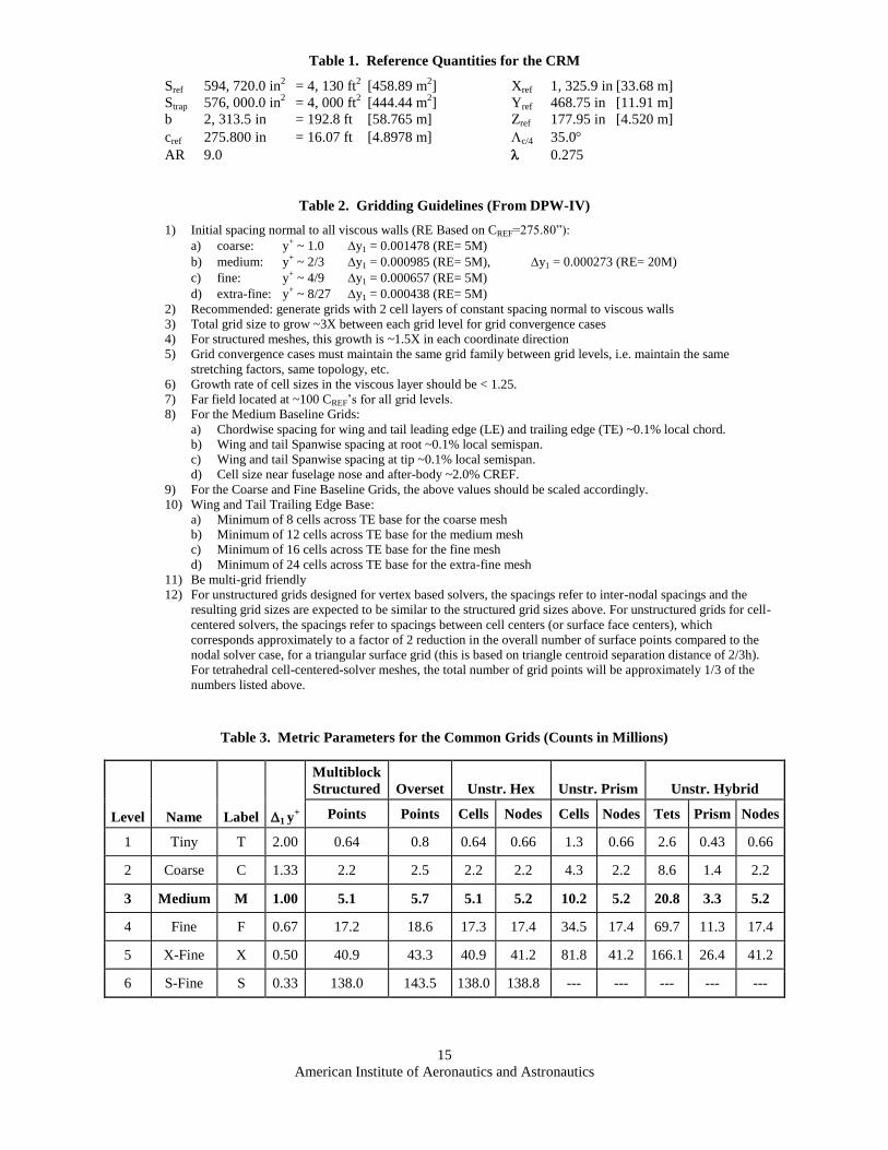
All participants were asked to submit force/moment, pressure, and separation data in a standard format. The

large number of datasets poses a challenge in the presentation of the data. Each dataset is assigned an Alphanumeric

(including Greek) symbol type while colors and line types are used to denote grid or turbulence model type

depending on context. All of the force/moment and pressure plots below follow the scheme listed in Table 4.

B. Case 1: CRM at Cruise Mach

The first test case is focused on the grid refinement study for the CRM Wing-Body at M=0.85 and CL=0.500.

The trends with grid size for total drag are shown in Figure 5, broken out by grid type and turbulence model.

Overall, the scatterband reduces considerably as the grid is refined, and the bulk of the results converge to a band

about 10-15 counts wide. The relatively poor agreement for the Tiny and Coarse grid levels is to be expected, as

they are below typical industry standards for grid resolution. There is no clear advantage of any one grid type in

terms of a reduced scatter. With one exception, similar trends can be observed for the turbulence models. The

Goldberg RT model (Datasets M, O, Q, and S) clearly predicts the drag to be higher, although some of the SST

results (T and P) with the same code are high as well. The two other sets from this team (N and P) which use the

SST model compare well with the other SST results. Most of the SST results have a shallower trend with grid size

and agree with each other very well even though they represent the results of six different codes and multiple grid

types. Similar trends are seen in the Skin Friction and Pressure drag components, Figure 6 and Figure 7. The skin

friction does not vary significantly with grid resolution, confirming that grid refinement beyond a certain level is not

needed to resolve the boundary layer for most of the grids and turbulence models. Alpha for CL=0.500 and pitching

moment are shown in Figure 8. Other than a few outliers, the trends are very flat with grid size. Alpha falls

generally in the range from 2.1-2.3, and the spread in pitching moment is ~0.02. The latter represents a stabilizer

incidence range of about 0.5 for typical tail configurations.

A standard technique in grid convergence studies is to use the Richardson Extrapolation. As implemented here,

a standard least squares curve fit is used with grid factor, N-2/3

, where N is the number of unknowns. For second

order codes the error should linearly decrease as long as the refinement extends into the asymptotic region. The Y-

intercept then estimates the theoretical infinite resolution (continuum) result. The extrapolations are shown in

Figure 9. It is clear that some nonlinearity is still present in the curves, which would indicate that the asymptotic

region has not yet been reached for the coarse grid levels because there are still changes in some flow features with

grid refinement. At finer levels the behavior is more linear.

Also shown here for the first time are wind tunnel results from the NASA NTF and Ames tests, which warrants

some discussion. Differences in the “test” set-up between Wind Tunnel and CFD are well known, and a few are

listed below:

Wind Tunnel CFD

Walls Free Air

Support System (Sting) Free Air

Laminar/Turbulent (Tripped) “Fully” Turbulent (usually)

Aeroelastic Deformation Rigid 1g Shape

Measurement Uncertainty Numerical Uncertainty and Error

Corrections for known effects No Corrections

8

American Institute of Aeronautics and Astronautics

Clearly there are potentially significant differences between what Wind Tunnel and CFD are measuring/computing.

It is important to assess differences in magnitude between wind tunnel and CFD, but until the above variables are

better addressed we should consider that the wind tunnel data are included for reference only.

As described above, the common grid study is a key feature of DPW-V. Figure 9a shows total drag coefficient

results for all grids, while Figure 9b shows only the Common Grids which use the exact same node distributions. A

quite significant variation in the solutions remains, which may be due to the cell subdivisions into prisms and

tetrahedra. So the data are further reduced to only hex-based grids – Structured, Unstructured, and Overset – in

Figure 9c. Any remaining variation must be due to specifics of the CFD method coding, including turbulence

model.

Figure 10a shows the angle of attack for CL=0.500, while Figure 10b shows the pitching moment. All the

methods predict alpha to be too low compared to the wind tunnel – a result that has been present in all previous

workshops. Part of the reason for this is wing aeroelastic bending, but it is likely not the entire reason. Pitching

moment is also too negative, also at least partly from wing bending.

The continuum drag estimates are shown in Figure 11. The spread in the drag coefficient is 27.9 counts, while

the standard deviation is 5.3 counts. These represent a small improvement from DPW-IV, which were 40.9 and 8.1

counts, respectively. Average and median CD are 0.02516 and 0.02496, the difference reflecting the skewed nature

of the distribution shown in the inset figure. The median solution is within about 4 counts of the wind tunnel data.

Although the exact magnitude of the differences between wind tunnel and CFD described above are not known, it is

still a good sign that the data agree reasonably well.

Pressure coefficients at six stations along the wing span are shown in Figure 12 for the Level 3 grid submissions.

The level of scatter and agreement with wind tunnel data are generally very good although both tend to deteriorate

as the span station progresses to the wing tip. The tunnel data tend to have lower leading edge suction peaks than

the CFD results. This trend may be the result of aeroelastic deformation of the wing on the wind tunnel model,

which would lower the tip incidence on a swept wing. Effects of grid refinement are shown in Figure 13 for Station

10 ( =.5024). Note that fewer pressure datasets were provided for Levels 1, 5, and 6, and that should be taken into

account as it magnifies the decrease in scatterband at higher grid resolutions. There is no fundamental change in

shock location with the finer grids. There are no observable trends with grid type or turbulence model in the pressure

distributions.

C. Case 2: CRM Buffet Study

The second mandatory case is based on a buffet study to investigate the CFD predictions in an angle-of-attack

range where significant flow separation is expected. This flight regime is of particular importance to determining

aerodynamic loads and stability and control characteristics. Seven angles-of-attack were specified between 2.5 and

4.0° at 0.25° increments. Computed results of lift, drag, pitching moment, wing section pressure and skin friction

coefficients at specified spanwise locations, and locations of flow separation on the wing and side of body were

requested at each angle-of-attack. Over 50 data sets were provided by the Workshop participants for Case 2.

In assessing the quality of computed results it is desirable to have corresponding experimental data available for

comparison. Unfortunately, the initial comparisons with experimental results from both the National Transonic

Facility and the NASA Ames 11 Foot Wind Tunnel were disappointing. Studies reported in Refs. 62 and 63 have

identified the primary causes for the disagreement between the computed and measured results. These included the

effects of the swept-strut mounting system and most importantly the geometry of the wing used in the computational

analysis. The CRM wing geometry used for both the Fourth and Fifth Drag Prediction Workshops was defined prior

to the building and testing of the CRM wind tunnel model. Ideally the computational geometry should include the

aeroelastic deformation of the experimental subject under the actual test conditions. This is not generally done at

each test condition, but should be if the best possible correlation is desired. Typically the wind tunnel model is

designed to deflect to the desired design shape at a single cruise point in terms of lift, Mach number, and dynamic

pressure. Most, if not all CFD is done on that shape. The current CRM wind tunnel model was built to the design

shape. The CRM geometry and grids represent the design shape, which in this case is the wind-off shape. During

actual test conditions the model will deform under load.

To provide some measure for comparison a set of “pseudo” wind tunnel data was created. These “pseudo” data

are based on NTF data for the wing-body configuration and computational results from Ref. 63 for a wing-body-tail

configuration. The Ref. 63 results were for solutions using the Workshop geometry and solutions using a wing

shape derived from the model deformation data from the NTF at the “cruise” conditions. NTF test data, “pseudo”

test data, and computational results for the original geometry and the geometry with the measured twist are shown in

Figure 14. The difference between the two computational solutions was applied to the NTF experimental results to

generate the “pseudo” test data. For lift, the computational results with the measured twist are in reasonable

9

American Institute of Aeronautics and Astronautics

agreement with the NTF data while the computational results using the Workshop geometry agrees well with the

“pseudo” test data. The pitching moment data is significantly different in that the available computational results

were for a wing-body-tail configuration while the test data is for a wing-body configuration. Nevertheless, to first

order, the pitching moment increment due to twist should be applicable. Based results from Reference 63, it is

anticipated that corrections for the effect of the wind tunnel model mounting system (if they have been available for

the wing-body configuration) would have further increased the lift slightly and made the pitching moment more

negative in the “pseudo” data. These “pseudo” data should somewhat represent what would have been measured if

the wind tunnel model had assumed the “design” shape at the “cruise” condition. For purposes of the buffet study

the drag differences were too small to warrant creating “pseudo” drag data.

Lift and pitching moment results from all the Workshop submittals, along with the “pseudo”, NTF, and Ames

test data are shown in Figure 15. Most of the solutions are clustered within a “fan” that gets progressively wider

with increasing angle-of-attack. The exceptions are a group of solutions based on the Goldberg RT turbulence

model, and those other solutions that also suffered an early massive flow separation.

All the solutions were examined to determine outliers, and if there was some defining characteristic that

determined the quality of the solution. The outliers were defined as solutions that exhibited a break in lift prior to 4°

angle-of-attack, or exhibited drag considerably outside the norm of the other solutions. Outliers were seen in

solutions from all grid families, and from SA, SST, and Goldberg RT turbulence models. Lift break, which is

indicative of a large increase in flow separation, occurred as early as 3° angle-of-attack in five solutions. Seven

solutions exhibited a lift break between 3.25 and 3.5°, and a further nine solutions at 3.75° angle-of-attack.

The source of the early break can be found by examining the separation data requested by the DPW organizing

committee and provided by most participants. There is a tendency for some codes to predict a large separation

bubble at the wing root trailing edge by the side of body (SOB), shown in Figure 16, while others preserved smooth

flow virtually all of the way to the trailing edge. The predicted SOB separation bubble in these cases is large

enough to be seen in the force and moment results, however the wind tunnel data do not exhibit any evidence of

flow separation at the first row of pressures located at BL=151, nor does it show an early lift break. All of the

solutions identified with a separation bubble size greater than BL=151 also exhibited a lift break below 4 angle of

attack and have been identified as outliers. This type of 3D corner flow separation continues to need more attention

in turbulence model development.

Eliminating all the outliers as defined above, we have 26 solutions with lift and pitching moment characteristics

shown in Figure 17. Even with all the outliers removed there is still an increasing spread of the lift and pitching

moment with increasing angle-of-attack. At 4° angle-of-attack the value of lift coefficient varies by 0.055 and the

spread in pitching moment coefficient is 0.042! Note that for lift the solutions based on the SST turbulence model

tend to be clustered at the lower half of the group and are closest to the “pseudo” test data. These solutions are also

characterized by a slightly more forward shock position compared to the SA solutions. The SA solutions, which

encompass several different flavors of the SA turbulence model, span the spread although most tend to be in the

higher portion of the group. The solutions based on the EARSM and LagRST turbulence model are somewhere in

the middle. Each one of these solutions on its own is a valid solution, yet as angle-of-attack increases and the

resulting degree of flow separation increases, the variation between solutions increases. Which, if any, is most

correct? Further inspection could identify and remove more outliers, but the spread is likely to remain.

The drag characteristics of the remaining solutions are shown in Figure 18. Also shown are test results from

three repeat runs at both the NTF and Ames wind tunnels. Details of these tests and a description of the corrections

applied to the experimental data can be found in Ref. 47. “Pseudo” drag is not shown in that the twist corrections

are of the same order as the spread between repeat runs and would add nothing to the comparison. The drag

characteristics are plotted in terms of the idealized profile drag defined as:

CDP = CD – CL2/ ( AR)

Plotting CDP instead of CD can be very useful as its variation with CL is significantly diminished, and therefore,

the scale of the plot can be greatly increased. The spread of the drag values is largely driven by the increasing

spread of lift with increasing angle-of-attack. Note that the spread of the drag values at low lift coefficients is of the

same order as the spread of the test data between the two tunnels.

The significant variations in lift and pitching moment seen in the various solutions at each angle-of-attack are

driven largely by shock location and by the amount of trailing edge separation. The pressure distributions shown in

Figure 19 give some insight into these characteristics. At 2.75° angle-of-attack, except for solutions based on the

Goldberg RT turbulence model, very little trailing edge separation, less than 2% chord, exists. The lift and pitching

moment variation here is driven mainly by differences in shock location. By 3.0° angle-of-attack, as seen in Figure

10

American Institute of Aeronautics and Astronautics

20, there is a significant amount of trailing edge separation for most solutions except for the one based on the

EARSM turbulence model - somewhat more separation for the SST solutions, more variation among the various

versions of the SA turbulence model. By 4.0° angle-of-attack, as seen in Figure 20, there is a massive amount of

trailing edge separation with significantly different patterns between solutions. There does not appear to be any

single clear pattern.

The chaotic situation at these high angles-of-attack may be physical as well as computational. One must ask if

steady Reynolds Averaged Navier-Stokes is adequate for modeling this flow regime. Will URANS (Unsteady

Reynolds Averaged Navier-Stokes) be adequate, or must one go to an eddy-resolving method such as DES

(Detached Eddy Simulation) to accurately simulate this flow regime? In addition to further CFD research in this

area, detailed experimental measurements that adequately capture the flow separation and unsteadiness on these type

configurations must also be acquired.

C. Case 3: Turbulence Model Verification Study

A unique feature of this drag prediction workshop was the addition of an optional set of simple test cases from

the online Turbulence Model Resource website61

. These test cases were designed to discriminate between

turbulence models and their coding implementations through rigorous grid convergence studies. In other words,

different CFD codes that have implemented a given turbulence model as intended should produce nearly the same

result as the grid is refined for these cases. This same type of rigorous verification testing is currently not possible

for complex configurations such as the CRM.

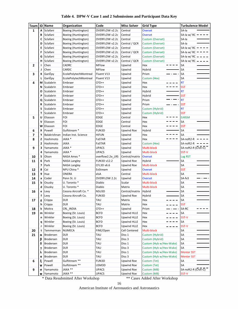
In this study, designated as Case 3, three 2-D cases were selected: flat plate, bump, and NACA 0012 airfoil.

Ten participants - representing 8 of the 21 teams who participated in cases 1 and 2 – submitted results, which were

compared with reference solutions from the online resource (using CFL3D). Table 5 summarizes the entries. For

convenience, a unique ID was assigned for these “turbulence modeling” cases. The table shows the linkage between

this ID and the corresponding ID(s) used in the CRM part of the workshop. One dataset (indicated by a *) was

corrected after the workshop, and two datasets (indicated by a **) were added after the workshop. Unfortunately,

several of the participants submitted the requested information on only a single grid level, so it is not clear where

their solutions were heading as the grids were refined. All participants used a version of either the SA or SST

turbulence models. Note that SST uses strain-based production terms, and SST-V uses vorticity-based approximate

production terms. In the table, the model(s) used are indicated, along with the grid levels employed (f=finest,

m=medium, c=coarse). All grids (except those used by T7) were the same structured / hexahedral grids, which were

successively coarsened by removing every other point in each coordinate direction.

Case 3.1 Flat Plate: The zero-pressure-gradient flat plate case was computed using M=0.2, ReL=5 million,

where L=1 nondimensional unit and the total plate length was 2L. Figure 21 shows wall skin friction coefficient

using SA at location x=0.97, as a function of h, a measure of average grid spacing. (The online website notes that

quantities of interest rarely converge consistently at second order in practice, even for a nominally second-order

code on these simple problems, so h is chosen here for convenience.) Although T1 and T3 only used a single grid

size, their results were clearly inconsistent with the majority of the results. T4 also only used a single grid size, but

its results agreed well with the collective. Although not shown here, Cf results at other locations followed a similar

trend.

Using SST, four different participants agreed well with each other as the grid was refined, Figure 22. (Note that

when computing the flat plate, SST and SST-V are indistinguishable because strain and vorticity are the same.) T1

was again noticeably different than the collective. T3 was not run using an SST model.

Case 3.2 Bump: The bump case was useful because it tested more features than the simple flat plate, including

the use of non-Cartesian geometry and grid topology, as well as non-zero pressure gradient. The bump itself (with

maximum nondimensional height of 0.05) extended from 0.3 < x < 1.2. The solid wall extended from 0 < x < 1.5.

Flow conditions were M=0.2 and Re=3 million per unit length.

Again, wall skin friction coefficient at particular locations were a useful metric for evaluating the expected

solution for a given turbulence model. Figure 23 shows Cf as a function of h for the SA model at x=0.6322. Results

at other locations yielded similar conclusions. Once again, T1 and T3 were outliers compared to the majority of

results. In addition, for this case T5, T6, and the original T2 submissions produced a noticeably different trend from

the collective. Subsequently, the reason for the discrepancy was discovered to be the method used to compute

minimum distance function (distance to the nearest wall). The T5, T6, and early T2 results used an approximate

method. For example, T2 summed the distance by following along grid lines. When grid lines are not exactly

normal to the surface, this procedure introduces errors. Subsequently using a more accurate computation of

minimum distance function, T2’s corrected result aligned well with the collective.

11

American Institute of Aeronautics and Astronautics

Figure 24 shows a close-up of skin friction coefficient over the bump (near its peak) for SA. All results except

T3 used the fine (f) grid. Although relatively small, the level of disagreement between participant results is clearly

visible. The Cf curves predicted by participants T2, T4, T10, and T11 are nearly indistinguishable.

For the bump case, the particular version of SST made a difference in results, as shown in Figure 25. Although

not significantly different, SST-V yielded slightly lower values of Cf at this location than SST. All participants

except for T1 were consistent with each other.

Case 3.3 Airfoil: The NACA 0012 case was computed at M=0.15, Re=6 million per unit chord, and three

different angles of attack: 0, 10, and 15 deg. Although this case represented a more aerodynamically realistic

configuration than the other two cases, it turned out to be more difficult to draw firm conclusions. It may be

necessary to include even finer grids than 1793x513 in future studies. Selected results are only shown here for

AoA=15 deg. General conclusions from other angles of attack were similar.

As shown in Figure 26, for the NACA 0012, all participant results – including T1 and T3 – appeared to be

consistent using the SA model, in spite of uncertainties in the particular results that did not include grid studies.

(Note that T7 used a custom grid with anisotropic h-adaptation and a discontinuous Galerkin algorithm. Thus, its

results are not straightforward to plot along with other results; it is not of the same family and its point count was not

provided. Currently, it is arbitrarily plotted using h of approximately 0.002.) For the SST and SST-V models in

Figure 27, the drag coefficient was consistent among the participants, but the lift coefficient exhibited larger

variation. However, the lift coefficient was also changing significantly with grid refinement, even on the finest grid,

so it is difficult to draw firm conclusions without a grid study that includes even finer grids. At this level of detail, it

was also impossible to detect different trends between SST and SST-V.

Although not shown, submitted results for NACA 0012 surface pressure coefficient and surface skin friction

coefficient were generally consistent among participants for a given turbulence model, with the exception of

participants T3 and T7. It is possible that these particular results were post-processed incorrectly for the workshop.

In summary, the turbulence model verification study was a very useful exercise. Using simple well-defined test

cases (flat plate and bump) along with grid convergence studies, potential differences in turbulence modeling

implementations were quickly uncovered. Use of a NACA 0012 airfoil test case was less enlightening, and may

require the use of finer grids in future studies. For the flat plate and bump cases, T1 and T3 were consistently

different from the collective. However, these participants did not perform grid studies, so it is not clear whether the

inconsistencies were due to modeling differences, discretization errors, or a combination of both. The study also

helped to isolate differences due to a particular cause: the use of an approximate minimum distance function. This

was shown to introduce errors that could be an important factor when using complex grids on realistic

configurations. The study further demonstrated that small but quantifiable differences can be expected between two

commonly used forms of the SST model. Using simple problems to isolate and identify these levels of disparities

may eventually help to explain why different codes yield different results when using ostensibly the same turbulence

model on complex problems like the CRM.

VI. Conclusions

The fifth AIAA CFD Drag Prediction Workshop was held in conjunction with the 30th AIAA Applied

Aerodynamics conference in June, 2012. The event was well attended by a diverse group of expert CFD

practitioners from four continents representing government, industry, academia, and commercial code development

institutions. This workshop focused on a common grid study for the NASA Common Research Model wing-body

configuration, including single point grid convergence and high-alpha buffet conditions. An optional turbulence

model verification study was also included.

A total of 57 Reynolds Average Navier Stokes datasets were provided on structured, overset, and unstructured

grids. Of these, 37 used common grids all derived from the identical field of points regardless of grid type. For the

Case 1 grid convergence study, a Richardson Extrapolation was performed to estimate continuum results. Total

scatter and standard deviation were reduced from DPW-IV. Comparison to wind tunnel data is reasonable, within

about 4 counts to the median solution. However, since the wind tunnel test and CFD problem setups are inherently

different, there is some question as to how well they should agree. There are no clear breakouts with grid type or

turbulence model, with the exception of the Goldberg RT model which predicted higher drag than the bulk of the

other solutions – especially for the coarser grids.

For the Case 2 buffet study, a set of outliers were observed that had uncharacteristically large wing trailing edge

separation at the side of body which contributed to an early lift break. This break is definitely not present in the

wind tunnel data. For the solutions minus the outliers, the grouping of forces was relatively tight at α=2.5. In

general, CM was predicted to be too negative, partly due to known geometry differences including steady aeroelastic

12

American Institute of Aeronautics and Astronautics

effects. The later effect is observed in the wing pressure distributions which agree well over the inboard wing but

deteriorate outboard. Variations in the forces spread significantly at α=4.0 due to differences in shock induced

separation predicted on the wing. It is not known whether the flow is steady for those conditions and whether steady

RANS methods are adequate. Studies with unsteady RANS or DES may be needed to confirm these effects, as well

as experiments designed to measure unsteady flows. The SOB separation bubble characteristic of the outlier

solutions needs further study and development of turbulence models for corner flow geometries.

The Case 3 turbulence model verification study showed generally consistent results for a given turbulence

model, although potential differences in the implementation of some models were uncovered. An approximate

minimum distance function was shown to cause differences that could be significant when computing on realistic

configurations. Using this type of simple problem can help to explain conflicting results when using the same

turbulence model in different codes.

VII. References

1. 1st AIAA CFD Drag Prediction Workshop, Anaheim, CA, June 2001, http://aaac.larc.nasa.gov/tsab/cfdlarc/aiaa-

dpw/Workshop1/workshop1.html, accessed 11 November 2012.

2. Redeker, G., “DLR-F4 Wing-Body Configuration,” A Selection of Experimental Test Cases for the Validation of CFD

Codes, number AR-303, pages B4.1–B4.21. AGARD, August 1994.

3. Levy, D. W., Vassberg, J. C., Wahls, R. A., Zickuhr, T., Agrawal, S., Pirzadeh, S., and Hemsch, M. J., “Summary of data

from the first AIAA CFD Drag Prediction Workshop,” AIAA Journal of Aircraft, 40(5):875–882, Sep–Oct 2003.

4. Hemsch, M. J., “Statistical Analysis of CFD Solutions from the Drag Prediction Workshop,” AIAA paper 2002-0842, 40th

AIAA Aerospace Sciences Meeting & Exhibit, Reno, NV, January 2002.

5. Rakowitz, M., Eisfeld, B., Schwamborn, D., and Sutcliffe, M., “Structured and Unstructured Computations on the DLR-F4

Wing-Body Configuration,” AIAA Journal of Aircraft, 40(2):256–264, 2003.

6. Mavriplis, D. J. and Levy, D. W., “Transonic Drag Predictions Using an Unstructured Multigrid Solver,” AIAA Journal of

Aircraft, 42(4):887–893, 2005.

7. Pirzadeh, S. Z. and Frink, N. T., “Assessment of the Unstructured Grid Software TetrUSS for Drag Prediction of the DLR-

F4 Configuration,” AIAA paper 2002-0839, 40th AIAA Aerospace Sciences Meeting & Exhibit, Reno, NV, January 2002.

8. Vassberg, J. C., Buning, P. G., and Rumsey, C. L., “Drag Prediction for the DLR-F4 Wing/Body Using OVERFLOW and

CFL3D on an Overset Mesh,” AIAA Paper 2002-0840, 40th AIAA Aerospace Sciences Meeting & Exhibit, Reno, NV,

January 2002.

9. 2nd AIAA CFD Drag Prediction Workshop, Orlando, FL, June 2003, http://aaac.larc.nasa.gov/tsab/cfdlarc/aiaa-

dpw/Workshop2/workshop2.html, accessed 11 November 2012.

10. Laflin, K. R., Vassberg, J. C., Wahls, R. A., Morrison, J. H., Brodersen, O., Rakowitz, M., Tinoco, E. N., and Godard, J.,

“Summary of Data from the Second AIAA CFD Drag Prediction Workshop,” AIAA Journal of Aircraft, 42(5):1165–1178,

2005.

11. Hemsch, M. and Morrison, J., “Statistical analysis of CFD solutions from 2nd Drag Prediction Workshop,” AIAA Paper

2004-0556, 42nd AIAA Aerospace Sciences Meeting and Exhibit, Reno, NV, January 2004.

12. Pfeiffer, N., “Reflections on the Second Drag Prediction Workshop,” AIAA Paper 2004-0557, 42nd AIAA Aerospace

Sciences Meeting and Exhibit, Reno, NV, January 2004.

13. Brodersen, O. P., Rakowitz, M., Amant, S., Larrieu, P., Destarac, D., and Suttcliffe, M., “Airbus, ONERA and DLR Results

from the Second AIAA Drag Prediction Workshop,” AIAA Journal of Aircraft, 42(4):932–940, 2005.

14. Langtry, R. B., Kuntz, M., and Menter, F., “Drag Prediction of Engine-Airframe Interference Effects with CFX-5,” AIAA

Journal of Aircraft, 42(6):1523–1529, 2005.

15. Sclafani, J., DeHaan, M. A., and Vassberg, J. C., “OVERFLOW Drag Predictions for the DLR-F6 Transport Configuration:

A DPW-II Case study,” AIAA Paper 2004-0393, 42nd AIAA Aerospace Sciences Meeting and Exhibit, Reno, NV, January

2004.

16. Rumsey, C. Rivers, M., and Morrison, J., “Study of CFD Variations on Transport Configurations from the 2nd AIAA Drag

Prediction Workshop,” AIAA Paper 2004-0394, 42nd AIAA Aerospace Sciences Meeting and Exhibit, Reno, NV, January

2004.

17. Wutzler, K., “Aircraft Drag Prediction using Cobalt,” AIAA Paper 2004-0395, 42nd AIAA Aerospace Sciences Meeting

and Exhibit, Reno, NV, January 2004.

18. May, G., Van derWeide, E., Jameson, A., and Shankaran, S., “Drag Prediction of the DLR-F6 Configuration,” AIAA Paper

2004-0396, 42nd AIAA Aerospace Sciences Meeting and Exhibit, Reno, NV, January 2004.

19. Kim, Y., Park, S., and Kwon, J., “Drag prediction of DLR-F6 using the turbulent Navier-Stokes calculations with

multigrid,” AIAA Paper 2004-0397, 42nd AIAA Aerospace Sciences Meeting and Exhibit, Reno, NV, January 2004.

20. Yamamoto, K., Ochi, A., Shima, E., and Takaki, R., “CFD Sensitivity to Drag prediction on DLR-F6 Configuration by

Structured Method and Unstructured Method,” AIAA Paper 2004-0398, 42nd AIAA Aerospace Sciences Meeting and

Exhibit, Reno, NV, January 2004.

21. Tinoco, E. and Su, T., “Drag Prediction with the Zeus/CFL3D System,” AIAA Paper 2004-0552, 42nd AIAA Aerospace

Sciences Meeting and Exhibit, Reno, NV, January 2004.

13

American Institute of Aeronautics and Astronautics

22. 3rd AIAA CFD Drag Prediction Workshop, San Francisco, CA, June 2006, http://aaac.larc.nasa.gov/tsab/cfdlarc/aiaa-

dpw/Workshop3/workshop3.html, accessed 11 November 2012.

23. Vassberg, J. C., Sclafani, A. J., and DeHaan, M. A., “A Wing-Body Fairing Design for the DLR-F6 Model: A DPW-III Case

Study,” AIAA Paper 2005-4730, AIAA 23rd Applied Aerodynamics Conference, Toronto, Canada, June 2005.

24. Vassberg, J. C., Tinoco, E. N., Mani, M., Brodersen, O. P., Eisfeld, B., Wahls, R. A., Morrison, J. H., Zickuhr, T., Laflin, K.

R., and Mavriplis, D. J., “Abridged Summary of the Third AIAA CFD Drag Prediction Workshop,” AIAA Journal of

Aircraft, 45(3):781–798, May–June 2008.

25. Vassberg, J. C., Tinoco, E. N., Mani, M., Brodersen, O. P., Eisfeld, B., Wahls, R. A., Morrison, J. H., Zickuhr, T., Laflin, K.

R., and Mavriplis, D. J., “Summary of DLR-F6 Wing-Body Data from the Third AIAA CFD Drag Prediction Workshop,”

RTO AVT-147 Paper 57, RTO AVT-147 Symposium, Athens, Greece, December 2007.

26. Morrison, J. H. and Hemsch, M. J., “Statistical Analysis of CFD Solutions from the Third AIAA Drag Prediction

Workshop,” AIAA Paper 2007-0254, 45th AIAA Aerospace Sciences Meeting and Exhibit, Reno, NV, January 2007.

27. Tinoco, E. Winkler, N., C., Mani, M., and Venkatakrishnan, V., “Structured and Unstructured Solvers for the 3rd CFD Drag

Prediction Workshop,” AIAA Paper 2007-0255, 45th AIAA Aerospace Sciences Meeting and Exhibit, Reno, NV, January

2007.

28. Mavriplis, D. J., “Results from the 3rd Drag Prediction Workshop Using the NSU3D Unstructured Mesh Solver,” AIAA

Paper 2007-0256, 45th AIAA Aerospace Sciences Meeting and Exhibit, Reno, NV, January 2007.

29. Sclafani, A. J., Vassberg, J. C., Harrison, N. A., DeHaan, M. A., Rumsey, C. L., Rivers, S. M., and Morrison, J. H., “Drag

Predictions for the DLR-F6 Wing/Body and DPW Wings Using CFL3D and OVERFLOW on an Overset Mesh,” AIAA

Paper 2007-0257, 45th AIAA Aerospace Sciences Meeting and Exhibit, Reno, NV, January 2007.

30. Brodersen, O., Eisfeld, B., Raddatz, J., and Frohnapfel, P., “DLR Results from the Third AIAA CFD Drag Prediction

Workshop,” AIAA Paper 2007-0259, 45th AIAA Aerospace Sciences Meeting and Exhibit, Reno, NV, January 2007.

31. Tinoco, E. N., Venkatakrishnan, V., Winkler, C., and Mani M., “Structured and Unstructured Solvers for the Third AIAA

CFD Drag Prediction Workshop,” AIAA Journal of Aircraft, 45(3):738–749, May–June 2008.

32. Mavriplis, D. J., “Third Drag Prediction Workshop Results Using NSU3D Unstructured Mesh Solver,” AIAA Journal of

Aircraft, 45(3):750–761, May–June 2008.

33. Sclafani, A. J., Vassberg, J. C., Harrison, N. A., Rumsey, C. L., Rivers, S. M., and Morrison, J. H., “CFL3D / OVERFLOW

Results for DLR-F6 Wing/Body and Drag Prediction Workshop Wing,” AIAA Journal of Aircraft, 45(3):762–780, May–

June 2008.

34. Murayama, M. and Yamamoto, K., “Comparison Study of Drag Prediction by Structured and Unstructured Mesh Method,”

AIAA Journal of Aircraft, 45(3):799–822, May–June 2008.

35. Brodersen, O., Eisfeld, B., Raddatz, J., and Frohnapfel, P., “DLR results from the third AIAA Computational Fluid

Dynamics Drag Prediction Workshop,” AIAA Journal of Aircraft, 45(3):823–836, May–June 2008.

36. Eliasson, P. and Peng, S.-H., “Drag Prediction for the DLR-F6 Wing-Body Configuration Using the Edge Solver,” AIAA

Journal of Aircraft, 45(3):837–847, May–June 2008.

37. Mavriplis, D. J., Vassberg, J. C., Tinoco, E. N., Mani, M., Brodersen, O. P., Eisfeld, B., Wahls, R. H., Morrison, J., Zickuhr,

T., Levy, D., and Murayama, M., “Grid quality and Resolution Issues from the Drag Prediction Workshop Series,” AIAA

Journal of Aircraft, 46(3):935–950, 2009.

38. 4th AIAA CFD Drag Prediction Workshop, San Antonio, TX, June 2009. http://aaac.larc.nasa.gov/tsab/cfdlarc/aiaa-

dpw/Workshop4/workshop4.html, aiaadpw@gmail.com, accessed 11 November 2012.

39. Vassberg, J. C., DeHaan, M. A., Rivers, S. M., and Wahls, R. A., “Development of a Common Research Model for Applied

CFD Validation Studies,” AIAA Paper 2008-6919, 26th AIAA Applied Aerodynamics Conference, Hawaii, HI, August

2008.

40. Rivers, M. and Dittberner, A., “Experimental Investigations of the NASA Common Research Model,” AIAA Paper 2010-

4218, 28th AIAA Applied Aerodynamics Conference, Chicago, IL, June 2010.

41. Rivers, M. and Dittberner, A., “Experimental Investigations of the NASA Common Research Model in the NASA Langley

National Transonic Facility and NASA Ames 11-Ft Transonic Wind Tunnel (Invited),” AIAA Paper 2011-1126, presented

at the 49th Aerospace Sciences Meeting, Orlando, FL, Jan 2011.

42. Common Research Model, http://commonresearchmodel.larc.nasa.gov/, Accessed 11 November 2012.

43. Vassberg, J., Tinoco, E., Mani, M., Rider, B., Zickuhr, T., Levy, D., Broderson, O., Eisfeld, B., Crippa, S., Wahls, R.,

Morrison, J., Mavriplis, D., Murayama, M., “Summary of the Fourth AIAA CFD Drag Prediction Workshop,” AIAA 2010-

4547, 28th AIAA Applied Aerodynamics Conference, Chicago, IL, June 2010.

44. Morrison, J., “Statistical Analysis of CFD Solutions from the Fourth Drag Prediction Workshop,” AIAA 2010-4673, 28th

AIAA Applied Aerodynamics Conference, Chicago, IL, June 2010.

45. Sclafani, A. J., Vassberg, J. C., Rumsey, C., DeHaan, M. A., and Pulliam, T. H., “Drag Prediction for the NASA CRM

Wing/Body/Tail Using CFL3D and OVERFLOW on an Overset Mesh,” AIAA Paper 2010-4219, 28th AIAA Applied

Aerodynamics Conference, Chicago, IL, June 2010.

46. Hue, D., Gazaix, M., and Esquieu, S., “Computational Drag and Moment Prediction of the DPW4 Configuration with elsA,”

AIAA Paper 2010-4220, 28th AIAA Applied Aerodynamics Conference, Chicago, IL, June 2010.

47. Mani, M., Rider, B. J., Sclafani, A. J., Winkler, C., Vassberg, J. C., Dorgan, A. J., Cary, A., and Tinoco, E. N., “RANS

Technology for Transonic Drag Prediction; a Boeing Perspective of the 4th Drag Prediction Workshop,” AIAA Paper 2010-

4221, 28th AIAA Applied Aerodynamics Conference, Chicago, IL, June 2010.

14

American Institute of Aeronautics and Astronautics

48. Yamamoto, K., Tanaka, K., and Murayama, M., “Comparison Study of Drag Prediction for the 4th CFD Drag Prediction

Workshop Using Structured and Unstructured Mesh Methods,” AIAA Paper 2010-4222, 28th AIAA Applied Aerodynamics

Conference, Chicago, IL, June 2010.

49. Brodersen, O., Crippa, S., Eisfeld, B., Keye, S., and Geisbauer, S., “DLR Results for the Fourth AIAA CFD Drag Prediction

Workshop,” AIAA Paper 2010-4223, 28th AIAA Applied Aerodynamics Conference, Chicago, IL, June 2010.

50. Eliasson, P., Peng, S., and Tysell, L., “Computations from the 4th Drag Prediction Workshop Using the Edge solver,” AIAA

Paper 2010-4548, 28th AIAA Applied Aerodynamics Conference, Chicago, IL, June 2010.

51. Li, G. and Zhou, Z., “Validation of a Multigrid-Based Navier-Stokes Solver for Transonic Flows,” AIAA Paper 2010-4549,

28th AIAA Applied Aerodynamics Conference, Chicago, IL, June 2010.

52. Mavriplis, D. J. and Long, M., “NSU3D Results for the Fourth AIAA Drag Prediction Workshop,” AIAA Paper 2010-4550,

28th AIAA Applied Aerodynamics Conference, Chicago, IL, June 2010.

53. Lee-Rausch, E., Hammond, E., Nielsen, E., Pirzadeh, S., and Rumsey C., “Application of the FUN3D Unstructured-Grid

Navier-Stokes Solver to the 4th AIAA Drag Prediction Workshop Cases,” AIAA Paper 2010-4551, 28th AIAA Applied

Aerodynamics Conference, Chicago, IL, June 2010.

54. Vos, J., Sanchi, S., Gehri, A., and Stephani, P., “DPW4 Results Using Different Grids, Including Near-Field/Far-Field Drag

Analysis,” AIAA Paper 2010-4552, 28th AIAA Applied Aerodynamics Conference, Chicago, IL, June 2010.

55. Hashimoto, A., Lahur, P., Murakami, K., and Aoyama, T., “Validation of Fully Automatic Grid Generation Method on

Aircraft Drag Prediction,” AIAA Paper 2010-4669, 28th AIAA Applied Aerodynamics Conference, Chicago, IL, June 2010.

56. Temmerman, L. and Hirsch, C., “Simulations of the CRM Configuration on Unstructured Hexahedral Grids: Lessons

Learned from the DPW-4 Workshop,” AIAA Paper 2010-4670, 28th AIAA Applied Aerodynamics Conference, Chicago,

IL, June 2010.

57. Chaffin, M. and Levy, D., “Comparison of Viscous Grid Layer Growth Rate of Unstructured Grids on CFD Drag Prediction

Workshop Results,” AIAA Paper 2010-4671, 28th AIAA Applied Aerodynamics Conference, Chicago, IL, June 2010.

58. Crippa, S., “Application of Novel Hybrid Mesh Generation Methodologies for Improved Unstructured CFD Simulations,”

AIAA Paper 2010-4672, 28th AIAA Applied Aerodynamics Conference, Chicago, IL, June 2010.

59. 5th AIAA CFD Drag Prediction Workshop, http://aaac.larc.nasa.gov/tsab/cfdlarc/aiaa-dpw/, aiaadpw@gmail.com, accessed

11 November 2012.

60. Vassberg, J. C., “A Unified Baseline Grid about the Common Research Model Wing-Body for the Fifth AIAA CFD Drag

Prediction Workshop,” AIAA Paper 2011-3508, 29th AIAA Applied Aerodynamics Conference, Honolulu, HI, June 2011.

61. Rumsey, C., “Langley Research Center Turbulence Modeling Resource”, http://turbmodels.larc.nasa.gov/, accessed 23 June

2012.

62. Rivers, M. and Hunter, C., “Support System Effects on the NASA Common Research Model,” AIAA Paper 2012-707,

January 2012.

63. Rivers, M., Hunter, C., and Campbell, R., “Further Investigation of the Support System Effects and Wing Twist on the

NASA Common Research Model,” AIAA Paper 2012-3209, June 2012.

15

American Institute of Aeronautics and Astronautics

Table 1. Reference Quantities for the CRM

Sref 594, 720.0 in2 = 4, 130 ft

2 [458.89 m

2] Xref 1, 325.9 in [33.68 m]

Strap 576, 000.0 in2 = 4, 000 ft

2 [444.44 m

2] Yref 468.75 in [11.91 m]

b 2, 313.5 in = 192.8 ft [58.765 m] Zref 177.95 in [4.520 m]

cref 275.800 in = 16.07 ft [4.8978 m] c/4 35.0

AR 9.0 0.275

Table 2. Gridding Guidelines (From DPW-IV)

1) Initial spacing normal to all viscous walls (RE Based on CREF=275.80”):

a) coarse: y+ ~ 1.0 y1 = 0.001478 (RE= 5M)

b) medium: y+ ~ 2/3 y1 = 0.000985 (RE= 5M), y1 = 0.000273 (RE= 20M)

c) fine: y+ ~ 4/9 y1 = 0.000657 (RE= 5M)

d) extra-fine: y+ ~ 8/27 y1 = 0.000438 (RE= 5M)

2) Recommended: generate grids with 2 cell layers of constant spacing normal to viscous walls

3) Total grid size to grow ~3X between each grid level for grid convergence cases

4) For structured meshes, this growth is ~1.5X in each coordinate direction

5) Grid convergence cases must maintain the same grid family between grid levels, i.e. maintain the same

stretching factors, same topology, etc.

6) Growth rate of cell sizes in the viscous layer should be < 1.25.

7) Far field located at ~100 CREF’s for all grid levels.

8) For the Medium Baseline Grids:

a) Chordwise spacing for wing and tail leading edge (LE) and trailing edge (TE) ~0.1% local chord.

b) Wing and tail Spanwise spacing at root ~0.1% local semispan.

c) Wing and tail Spanwise spacing at tip ~0.1% local semispan.

d) Cell size near fuselage nose and after-body ~2.0% CREF.

9) For the Coarse and Fine Baseline Grids, the above values should be scaled accordingly.

10) Wing and Tail Trailing Edge Base:

a) Minimum of 8 cells across TE base for the coarse mesh

b) Minimum of 12 cells across TE base for the medium mesh

c) Minimum of 16 cells across TE base for the fine mesh

d) Minimum of 24 cells across TE base for the extra-fine mesh

11) Be multi-grid friendly

12) For unstructured grids designed for vertex based solvers, the spacings refer to inter-nodal spacings and the

resulting grid sizes are expected to be similar to the structured grid sizes above. For unstructured grids for cell-

centered solvers, the spacings refer to spacings between cell centers (or surface face centers), which

corresponds approximately to a factor of 2 reduction in the overall number of surface points compared to the

nodal solver case, for a triangular surface grid (this is based on triangle centroid separation distance of 2/3h).

For tetrahedral cell-centered-solver meshes, the total number of grid points will be approximately 1/3 of the

numbers listed above.

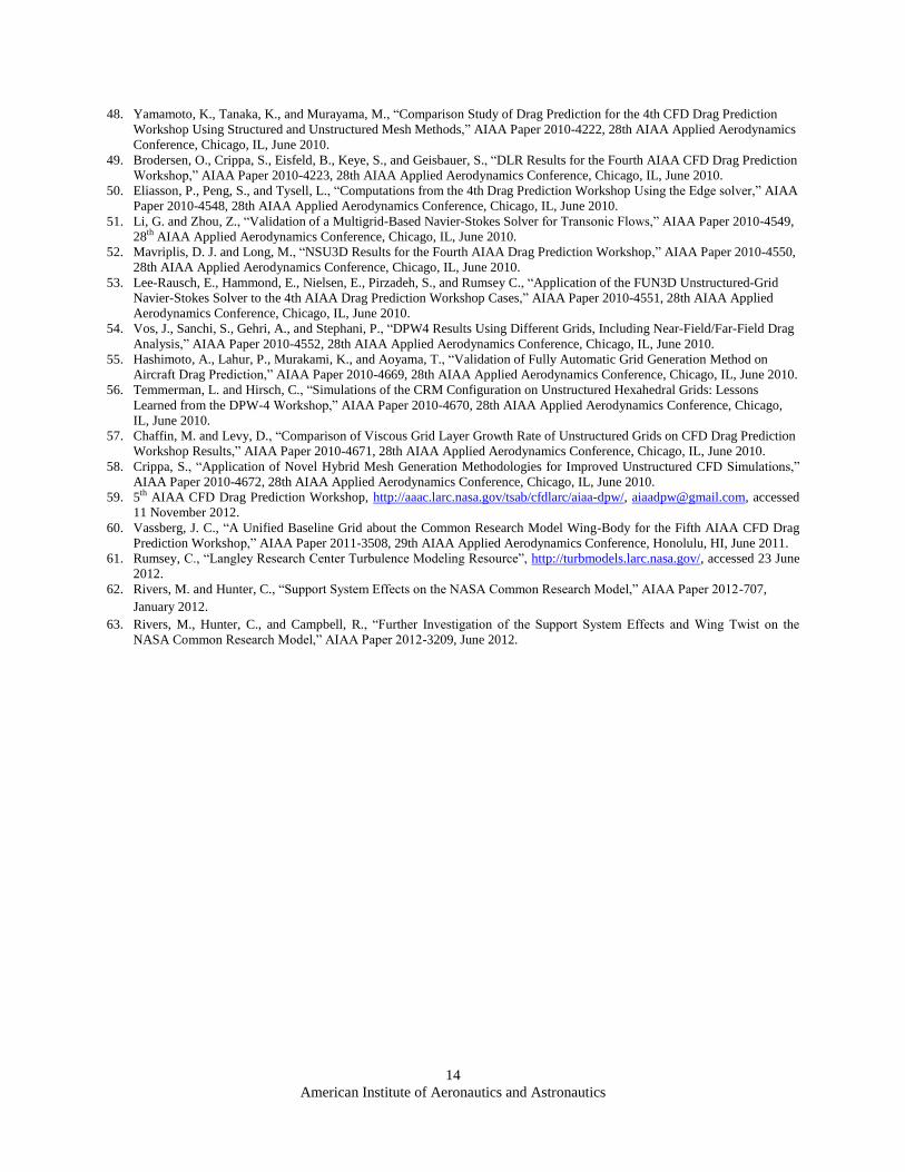
Table 3. Metric Parameters for the Common Grids (Counts in Millions)

Level Name Label 1 y+

Multiblock

Structured Overset Unstr. Hex Unstr. Prism Unstr. Hybrid

Points Points Cells Nodes Cells Nodes Tets Prism Nodes

1 Tiny T 2.00 0.64 0.8 0.64 0.66 1.3 0.66 2.6 0.43 0.66

2 Coarse C 1.33 2.2 2.5 2.2 2.2 4.3 2.2 8.6 1.4 2.2

3 Medium M 1.00 5.1 5.7 5.1 5.2 10.2 5.2 20.8 3.3 5.2

4 Fine F 0.67 17.2 18.6 17.3 17.4 34.5 17.4 69.7 11.3 17.4

5 X-Fine X 0.50 40.9 43.3 40.9 41.2 81.8 41.2 166.1 26.4 41.2

6 S-Fine S 0.33 138.0 143.5 138.0 138.8 --- --- --- --- ---

16

American Institute of Aeronautics and Astronautics

Table 4. DPW-V Case 1 and 2 Submissions and Participant Data Key

* Data Resubmitted After Workshop ** Cases Added After Workshop

Team ID Name Organization Code Misc Solver Grid Type Turbulence Model

A Sclafani Boeing (Huntington) OVERFLOW v2.2c Central Overset SA-Ia

B Sclafani Boeing (Huntington) OVERFLOW v2.2c Central Overset SA-Ia w/ RC

C Sclafani Boeing (Huntington) OVERFLOW v2.2c Central Custom (Overset) SA-Ia

D Sclafani Boeing (Huntington) OVERFLOW v2.2c Central / QCR Custom (Overset) SA-Ia

E Sclafani Boeing (Huntington) OVERFLOW v2.2c Central Custom (Overset) SA-Ia w/ RC

F Sclafani Boeing (Huntington) OVERFLOW v2.2c Central / QCR Custom (Overset) SA-Ia w/ RC

G Sclafani Boeing (Huntington) OVERFLOW v2.2c Central Custom (Overset) SA-Ia w/ RC

H Sclafani Boeing (Huntington) OVERFLOW v2.2c Central / QCR Custom (Overset) SA-Ia w/ RC

I Chen CADRC MFlow Upwind Hex SA

J Chen CARDC MFlow Upwind Hybrid SA

K GariÈpy EcolePolytechMontreal Fluent V13 Upwind Prism SA

L GariÈpy EcolePolytechMontreal Fluent V13 Upwind Custom (Hex) SA

M Scalabrin Embraer CFD++ Upwind Hex RT

N Scalabrin Embraer CFD++ Upwind Hex SST

O Scalabrin Embraer CFD++ Upwind Hybrid RT

P Scalabrin Embraer CFD++ Upwind Hybrid SST

Q Scalabrin Embraer CFD++ Upwind Prism RT

R Scalabrin Embraer CFD++ Upwind Prism SST

S Scalabrin Embraer CFD++ Upwind Custom (Hybrid) RT

T Scalabrin Embraer CFD++ Upwind Custom (Hybrid) SST

U Eliasson FOI EDGE Central Hex EARSM

V Eliasson FOI EDGE Central Hex SA

W Eliasson FOI EDGE Central Hex SST

6 X Powell Gulfstream * FUN3D Upwind Roe Hybrid SA

7 Y Balakrishnan Indian Inst. Science HiFUN Upwind Hex SA

Z Hashimoto JAXA * FaSTAR Upwind Hex SA-noft2-R

2 Hashimoto JAXA FaSTAR Upwind Custom (Hex) SA-noft2-R

3 Yamamoto JAXA * UPACS Upwind Multi-block SA-noft2-R (Crot=1)

4 Yamamoto JAXA * UPACS Upwind Multi-block SST-V

10 5 Olson NASA Ames * overflow2.2e_LRS Central/matrix Overset Lag RST

6 Park NASA Langley FUN3D v12.2 Upwind Roe Hybrid SA

7 Park NASA Langley CFL3D v6.6 Upwind Roe Multi-block SA

12 8 Cai NPU China * ExStream Upwind Overset SST

13 9 Hue ONERA elsA Central Multi-block SA

14 a Coder Penn St. U OVERFLOW 2.2c Upwind Overset SA-fv3

b Osusky U. Toronto * Diablo Scalar Multi-block SA

d Osusky U. Toronto * Diablo Matrix Multi-block SA

e Levy Cessna Aircraft Co. * NSU3D Central/matrix Hybrid SA

f Levy Cessna Aircraft Co. FUN3D Upwind Roe Hybrid SA

g Crippa DLR TAU Matrix Hex SA

h Crippa DLR TAU Matrix Hex SST

18 k Moitra CRL_INDIA CFD++ Upwind Prism SA-RC

m Winkler Boeing (St. Louis) BCFD Upwind HLLE Hex SA

n Winkler Boeing (St. Louis) BCFD Upwind HLLE Hex SST-V

q Winkler Boeing (St. Louis) BCFD Upwind HLLE Hex SA

r Winkler Boeing (St. Louis) BCFD Upwind HLLE Hex SST-V

20 t Temmerman NUMECA FINE/Open Cell Centered Multi-block SA

Brodersen DLR TAU Diss 1 Custom (Hybrid) SA

b Brodersen DLR TAU Diss 3 Custom (Hybrid) SA

d Brodersen DLR TAU Diss 1 Custom (Hyb w/Hex-Wake) SA

g Brodersen DLR TAU Diss 3 Custom (Hyb w/Hex-Wake) SA

Brodersen DLR TAU Diss 1 Custom (Hyb w/Hex-Wake) Menter SST

Brodersen DLR TAU Diss 3 Custom (Hyb w/Hex-Wake) Menter SST

x Powell Gulfstream ** FUN3D Upwind Roe Custom (Tet) SA

y Powell Gulfstream ** USM3D Upwind Roe Custom (Tet) SA

s Yamamoto JAXA ** UPACS Upwind Roe Custom (MB) SA-noft2-R (Crot=1)

v Yamamoto JAXA ** UPACS Upwind Roe Custom (MB) SST-V

17

19

21

6

9

16

1

2

3

4

5

8

9

11

15

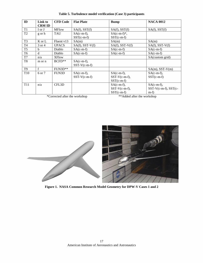
17

American Institute of Aeronautics and Astronautics

Table 5. Turbulence model verification (Case 3) participants

ID Link to

CRM ID

CFD Code Flat Plate Bump NACA 0012

T1 I or J MFlow SA(f), SST(f) SA(f), SST(f) SA(f), SST(f)

T2 g or h TAU SA(c-m-f),

SST(c-m-f)

SA(c-m-f)*,

SST(c-m-f)

T3 K or L Fluent v13 SA(m) SA(m) SA(m)

T4 3 or 4 UPACS SA(f), SST-V(f) SA(f), SST-V(f) SA(f), SST-V(f)

T5 b Diablo SA(c-m-f) SA(c-m-f) SA(c-m-f)

T6 d Diablo SA(c-m-f) SA(c-m-f) SA(c-m-f)

T7 n/a XFlow SA(custom grid)

T8 m or n BCFD** SA(c-m-f),

SST-V(c-m-f)

T9 f FUN3D** SA(m), SST-V(m)

T10 6 or 7 FUN3D SA(c-m-f),

SST-V(c-m-f)

SA(c-m-f),

SST-V(c-m-f),

SST(c-m-f)

SA(c-m-f),

SST(c-m-f)

T11 n/a CFL3D SA(c-m-f),

SST-V(c-m-f),

SST(c-m-f)

SA(c-m-f),

SST-V(c-m-f), SST(c-

m-f)

*Corrected after the workshop **Added after the workshop

Figure 1. NASA Common Research Model Geometry for DPW-V Cases 1 and 2

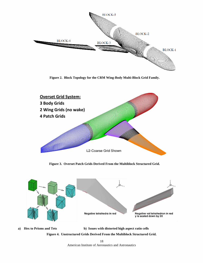
18

American Institute of Aeronautics and Astronautics

Figure 2. Block Topology for the CRM Wing-Body Multi-Block Grid Family.

Figure 3. Overset Patch Grids Derived From the Multiblock Structured Grid.

a) Hex to Prisms and Tets b) Issues with distorted high aspect ratio cells

Figure 4. Unstructured Grids Derived From the Multiblock Structured Grid.

Overset Grid System:

3 Body Grids

2 Wing Grids (no wake)

4 Patch Grids

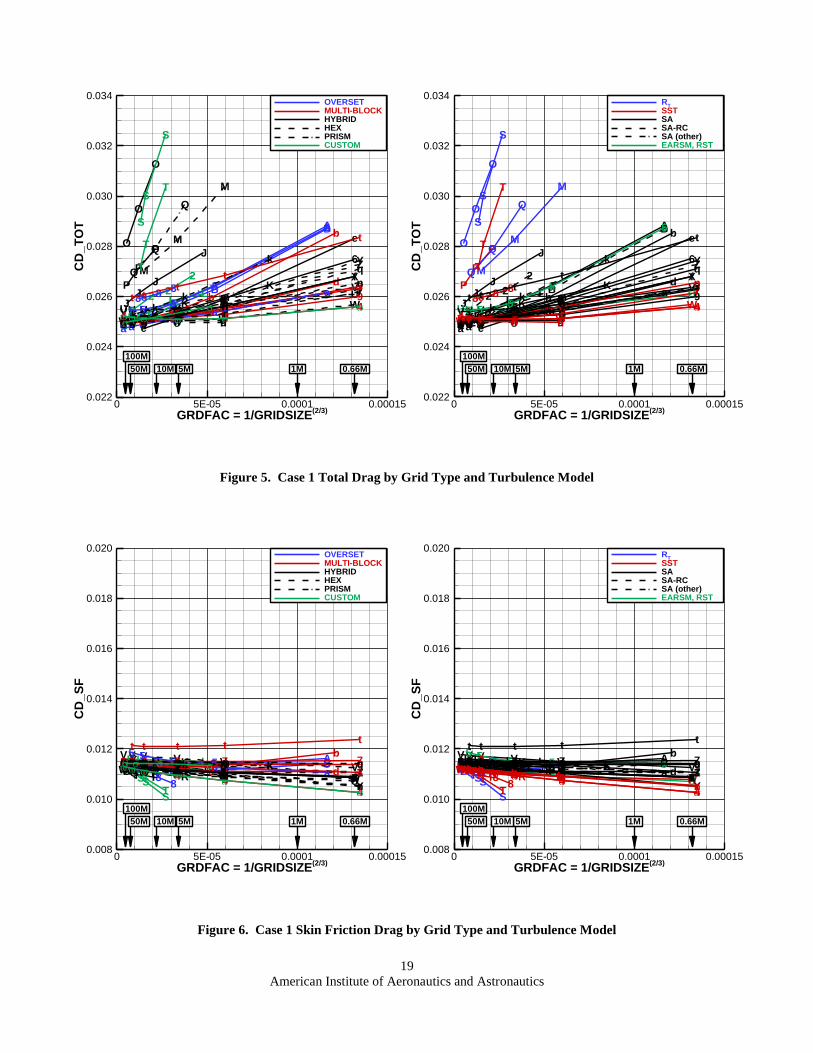
19

American Institute of Aeronautics and Astronautics

Figure 5. Case 1 Total Drag by Grid Type and Turbulence Model

Figure 6. Case 1 Skin Friction Drag by Grid Type and Turbulence Model

A

A

AA

B

B

BBBB

EE

EE

I

IIII

J

JJ

J

K

KKK

LL

LL

M

M

M

NNN

O

O

OP

P

P

Q

Q

Q

RRR

S

S

S

T

T

T

U

UUUUU

V

VVVVVW

WWWWW

X

XXXX

Y

YY

YY

Z

ZZ

ZZZ

2

22

2

3

33333

444444

5

5

555

6

6

666

7

7777

8888 9

99999

a

aa

aaa

b

b

bbbb

d

ddddd

e

e

ee

f

ffff ggggg hhhhh

k

kk

k

mm

mm

n

nnnn

q

qq

qq

r

rrrr

t

tt

tts

sss

vvvvvv

0.66M1M5M10M50M

100M

GRDFAC = 1/GRIDSIZE(2/3)

CD

_T

OT

0 5E-05 0.0001 0.000150.022

0.024

0.026

0.028

0.030

0.032

0.034OVERSETMULTI-BLOCKHYBRIDHEXPRISMCUSTOM

A

A

AA

B

B

BBBB

EE

EE

I

IIII

J

JJ

J

K

KKK

LL

LL

M

M

M

NNN

O

O

OP

P

P

Q

Q

Q

RRR

S

S

S

T

T

T

U

UUUUU

V

VVVVVW

WWWWW

X

XXXX

Y

YY

YY

Z

ZZ

ZZZ

2

22

2

3

33333

444444

5

5

555

6

6

666

7

7777

8888 9

99999

a

aa

aaa

b

b

bbbb

d

ddddd

e

e

ee

f

ffff ggggg hhhhh

k

kk

k

mm

mm

n

nnnn

q

qq

qq

r

rrrr

t

tt

tts

sss

vvvvvv

0.66M1M5M10M50M

100M

GRDFAC = 1/GRIDSIZE(2/3)

CD

_T

OT

0 5E-05 0.0001 0.000150.022

0.024

0.026

0.028

0.030

0.032

0.034R

T

SSTSASA-RCSA (other)EARSM, RST

AAAA BBBBBB EEEE I

IIIIJJJJ KKKK LLLL

MMM NNNO

OOPPP

QQQ RRR

S

SS

TTT

UUUUUU VVVVVV

WWWWWWX

XXXX

YY

YYYZZZZZZ 2222333333

44

4444 55555

66666 77777

88

88 999999

aaaaaa

b

bbbbbdddddd

eeeef

ffff ggggg

hhhhh kkkk mmmm

nnnnn qqqqq

rrrrr

ttttt

ssss

vv

vvvv

0.66M1M5M10M50M

100M

GRDFAC = 1/GRIDSIZE(2/3)

CD

_S

F

0 5E-05 0.0001 0.000150.008

0.010

0.012

0.014

0.016

0.018

0.020OVERSETMULTI-BLOCKHYBRIDHEXPRISMCUSTOM

AAAA BBBBBB EEEE I

IIIIJJJJ KKKK LLLL

MMM NNNO

OOPPP

QQQ RRR

S

SS

TTT

UUUUUU VVVVVV

WWWWWWX

XXXX

YY

YYYZZZZZZ 2222333333

44

4444 55555

66666 77777

88

88 999999

aaaaaa

b

bbbbbdddddd

eeeef

ffff ggggg

hhhhh kkkk mmmm

nnnnn qqqqq

rrrrr

ttttt

ssss

vv

vvvv

0.66M1M5M10M50M

100M

GRDFAC = 1/GRIDSIZE(2/3)

CD

_S

F

0 5E-05 0.0001 0.000150.008

0.010

0.012

0.014

0.016

0.018

0.020R

T

SSTSASA-RCSA (other)EARSM, RST

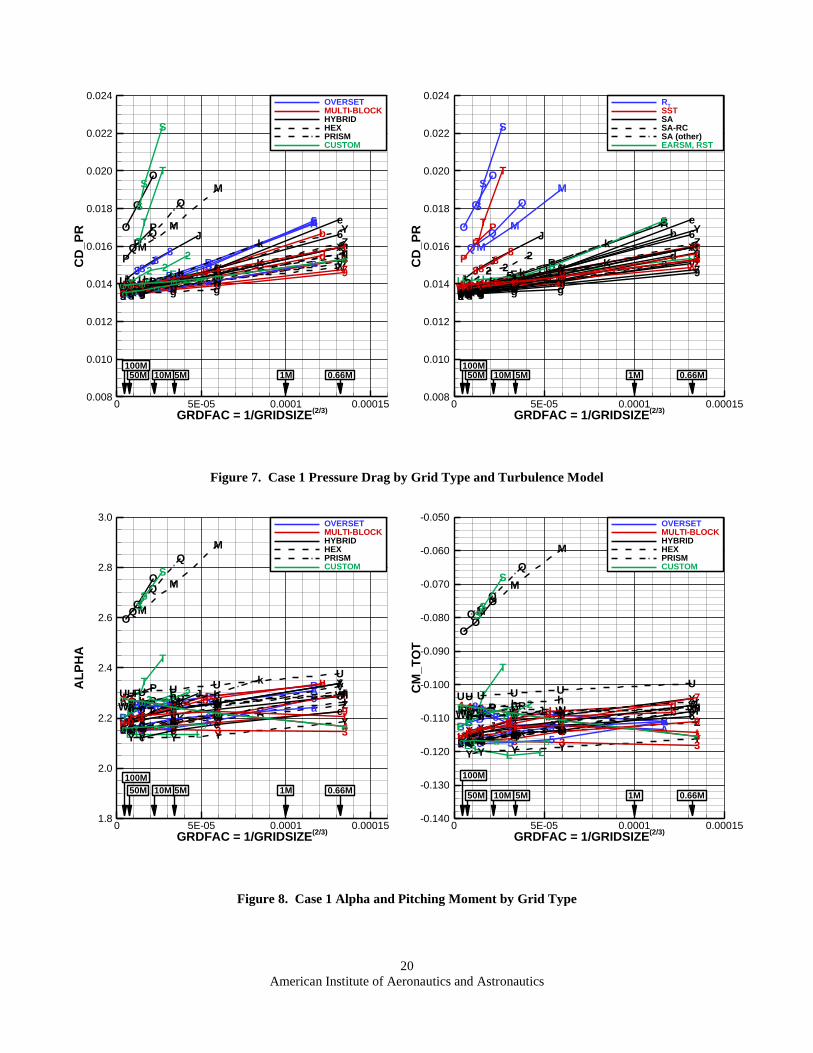
20

American Institute of Aeronautics and Astronautics

Figure 7. Case 1 Pressure Drag by Grid Type and Turbulence Model

Figure 8. Case 1 Alpha and Pitching Moment by Grid Type

A

A

AA

B

B

BBBB

EE

EE

I

IIII

J

JJ

J

K

KKK

LL

LL

M

M

M

NNN

O

O

O P

P

P

Q

Q

Q

RRR

S

S

S

T

T

T

U

UUUUU

V

VVVVV

WWWWWW

X

XX

XX

Y

Y

YYY

Z

ZZ

ZZZ

222

2

3

33333

4

44444

5

5

555

6

66

66

7

7777

88

88 9

99999

a

aaaaa

b

bb

bbb

d

ddddd

e

e

ee

f

ff

ff ggggghhhhh

k

kk

k

mm

mm

n

nnnn

q

qq

qq

r

rrrr

t

tt

tts

sss

v

vvvvv

0.66M1M5M10M50M100M

GRDFAC = 1/GRIDSIZE(2/3)

CD

_P

R

0 5E-05 0.0001 0.000150.008

0.010

0.012

0.014

0.016

0.018

0.020

0.022

0.024OVERSETMULTI-BLOCKHYBRIDHEXPRISMCUSTOM

A

A

AA

B

B

BBBB

EE

EE

I

IIII

J

JJ

J

K

KKK

LL

LL

M

M

M

NNN

O

O

O P

P

P

Q

Q

Q

RRR

S

S

S

T

T

T

U

UUUUU

V

VVVVV

WWWWWW

X

XX

XX

Y

Y

YYY

Z

ZZ

ZZZ

222

2

3

33333

4

44444

5

5

555

6

66

66

7

7777

88

88 9

99999

a

aaaaa

b

bb

bbb

d

ddddd

e

e

ee

f

ff

ff ggggghhhhh

k

kk

k

mm

mm

n

nnnn

q

qq

qq

r

rrrr

t

tt

tts

sss

v

vvvvv

0.66M1M5M10M50M100M

GRDFAC = 1/GRIDSIZE(2/3)

CD

_P

R0 5E-05 0.0001 0.00015

0.008

0.010

0.012

0.014

0.016

0.018

0.020

0.022

0.024R

T

SSTSASA-RCSA (other)EARSM, RST

AA

AA

BB

BBBB

EE

EE

I

IIII

J

JJJ

KKKK

LLLL

M

M

M

NNN

O

O

O

PPP

Q

Q

Q

RRR

S

SS

T

T

T

UUUUUU

V

VV

VVV

WWWWWW

X

XX

XX Y

YYYY

Z

ZZZZZ

222

2

333333 4

44

444 5

5555

6

6666

7

77

77

88889

99999

aaa

aaa

b

bb

bbb

d

dd

ddde

ee

e

f

ff

ff ggggg

hhhhh

k

kk

k mm

mm

nnnnn

q

qqqq

r

rrrrttttt

ssss v

vv

vvv

0.66M1M5M10M50M

100M

GRDFAC = 1/GRIDSIZE(2/3)

AL

PH

A

0 5E-05 0.0001 0.000151.8

2.0

2.2

2.4

2.6

2.8

3.0OVERSETMULTI-BLOCKHYBRIDHEXPRISMCUSTOM

AAAAB

BBBBB

EE

EE

I

IIII

J

JJJ

KKKK

LLLL

M

M

M

NNN

O

OO

PPP

Q

Q

Q

RRR

S

SS

T

T

T

UUUUUU

V

VV

VVV

WWWWWW

X

XX

XXY

YYYY

ZZZZZZ

222

2

333333 4

44

444

5

5555

66666

7

77

77

88

88

99

9999

aaa

aaa

bbb

bbb

dd

dddd

e

eee

f

ff

ffg

gggg

hhhhh

mm

mm

nnnnn

q

qq

qq

rrrrr

ttttt

ssssv

vv

vvv

0.66M1M5M10M50M

100M

GRDFAC = 1/GRIDSIZE(2/3)

CM

_T

OT

0 5E-05 0.0001 0.00015-0.140

-0.130

-0.120

-0.110

-0.100

-0.090

-0.080

-0.070

-0.060

-0.050OVERSETMULTI-BLOCKHYBRIDHEXPRISMCUSTOM

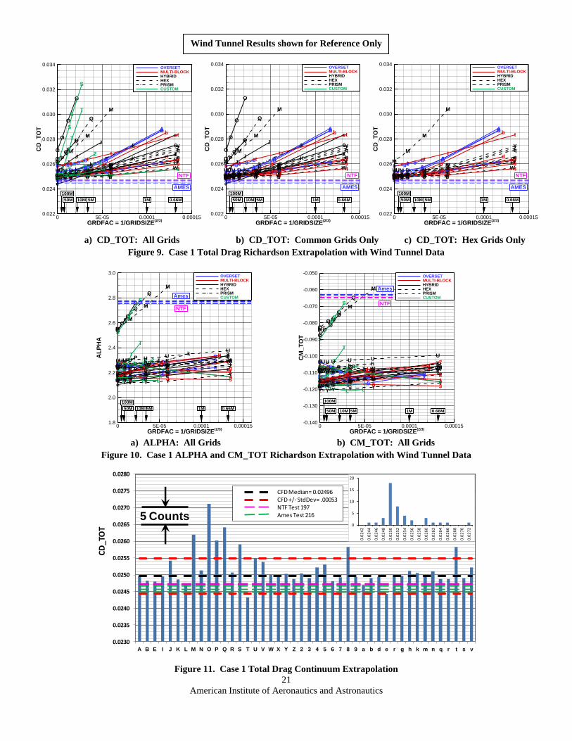
21

American Institute of Aeronautics and Astronautics

a) CD_TOT: All Grids b) CD_TOT: Common Grids Only c) CD_TOT: Hex Grids Only

Figure 9. Case 1 Total Drag Richardson Extrapolation with Wind Tunnel Data

a) ALPHA: All Grids b) CM_TOT: All Grids

Figure 10. Case 1 ALPHA and CM_TOT Richardson Extrapolation with Wind Tunnel Data

Figure 11. Case 1 Total Drag Continuum Extrapolation

A

A

AA

A

B

B

BBBBB

EE

EEE

I

IIIII

J

JJ

JJ

K

KKK

K

LL

LLL

M

M

M

M

NNNN

O

O

O

O

P

P

PP

Q

Q

Q

Q

RRRR

S

S

S

S

T

T

T

T

U

UUUUUU

V

VVVVVVW

WWWWWW

X

XXXXX

Y

YY

YYY

Z

ZZ

ZZZZ

2

22

22

3

333333

4444444

5

5

5555

6

6

6666

7

77777

88888 9

999999

a

aa

aaaa

b

b

bbbbb

d

dddddd

e

e

ee

e

f

fffff gggggg hhhhhh

k

kk

kk

mm

mmm

n

nnnnn

q

qq

qqq

r

rrrrr

t

tt

ttts

ssss

vvvvvvv

0.66M1M5M10M50M

100M

NTF

AMES

GRDFAC = 1/GRIDSIZE(2/3)

CD

_T

OT

0 5E-05 0.0001 0.000150.022

0.024

0.026

0.028

0.030

0.032

0.034OVERSETMULTI-BLOCKHYBRIDHEXPRISMCUSTOM

A

A

AA

A

B

B

BBBBB

I

IIIII

J

JJ

JJ

K

KKK

K

M

M

M

M

NNNN

O

O

O

O

P

P

PP

Q

Q

Q

Q

RRRR

U

UUUUUU

V

VVVVVVW

WWWWWW

X

XXXXX

Y

YY

YYY

Z

ZZ

ZZZZ

3

333333

4444444

5

5

5555

6

6

6666

7

77777

88888 9

999999

a

aa

aaaa

b

b

bbbbb

d

dddddd

e

e

ee

e

f

fffff gggggg hhhhhh

k

kk

kk

mm

mmm

n

nnnnn

q

qq

qqq

r

rrrrr

t

tt

ttt

0.66M1M5M10M50M

100M

NTF

AMES

GRDFAC = 1/GRIDSIZE(2/3)

CD

_T

OT

0 5E-05 0.0001 0.000150.022

0.024

0.026

0.028

0.030

0.032

0.034OVERSETMULTI-BLOCKHYBRIDHEXPRISMCUSTOM

A

A

AA

A

B

B

BBBBB

I

IIIII

M

M

M

M

NNNN

U

UUUUUU

V

VVVVVVW

WWWWWW

Y

YY

YYY

Z

ZZ

ZZZZ

3

333333

4444444

5

5

5555

7

77777

88888 9

999999

a

aa

aaaa

b

b

bbbbb

d

dddddd gggggg hhhhhh

mm

mmm

n

nnnnn

q

qq

qqq

r

rrrrr

t

tt

ttt

0.66M1M5M10M50M

100M

NTF

AMES

GRDFAC = 1/GRIDSIZE(2/3)

CD

_T

OT

0 5E-05 0.0001 0.000150.022

0.024

0.026

0.028

0.030

0.032

0.034OVERSETMULTI-BLOCKHYBRIDHEXPRISMCUSTOM

AA

AA

A

BB

BBBBB

EE

EEE

I

IIIII

J

JJJJ

KKKK

K LLLLL

M

M

M

M

NNNN

O

O

O

O

PPPP

Q

Q

Q

Q

RRRR

S

SS

S

T

T

T

T

UUUUUUU

V

VV

VVVV

WWWWWWW

X

XX

XXX Y

YYYYY

Z

ZZZZZZ

222

22

3333333 4

44

4444 5

55555

6

66666

7

77

777

888889

999999

aaa

aaaa

b

bb

bbbb

d

dd

dddd

e

ee

ee

f

ff

fffgg

gggg

hhhhhh

k

kk

kkm

mmmm

nnnnnn

q

qqqqq

r

rrrrrtttttt

sssss v

vv

vvvv

0.66M1M5M10M50M

100M

Ames

NTF

GRDFAC = 1/GRIDSIZE(2/3)

AL

PH

A

0 5E-05 0.0001 0.000151.8

2.0

2.2

2.4

2.6

2.8

3.0OVERSETMULTI-BLOCKHYBRIDHEXPRISMCUSTOM

AAAAAB

BBBBBB

EE

EEE

I

IIIII

J

JJJJ

KKKKK

LLLL

L

M

M

M

M

NNNN

O

OO

O

PPPP

Q

Q

QQ

RRRR

S

SS

S

T

T

T

T

UUUUUUU

V

VV

VVVV

WWWWWWW

X

XX

XXXY

YYYYY

ZZZZZZZ

222

22

3333333 4

44

4444

5

55555

666666

7

77

777

88

888

99

99999

aaa

aaaa

bbb

bbbb

dd

ddddd

e

eeee

f

ff

fffg

ggggg

hhhhhh

mm

mmm

nnnnnn

q

qq

qqq

rrrrrr

tttttt

sssssv

vv

vvvv

0.66M1M5M10M50M

100M

Ames

NTF

GRDFAC = 1/GRIDSIZE(2/3)

CM

_T

OT

0 5E-05 0.0001 0.00015-0.140

-0.130

-0.120

-0.110

-0.100

-0.090

-0.080

-0.070

-0.060

-0.050OVERSETMULTI-BLOCKHYBRIDHEXPRISMCUSTOM

0.0230

0.0235

0.0240

0.0245

0.0250

0.0255

0.0260

0.0265

0.0270

0.0275

0.0280

A B E I J K L M N O P Q R S T U V W X Y Z 2 3 4 5 6 7 8 9 a b d e r g h k m n q r t s v

CD

_TO

T

CFD Median= 0.02496CFD +/- StdDev= .00053NTF Test 197Ames Test 2165 Counts

Wind Tunnel Results shown for Reference Only

0

5

10

15

20

0.0

24

2

0.0

24

4

0.0

24

6

0.0

24

8

0.0

25

0

0.0

25

2

0.0

25

4

0.0

25

6

0.0

25

8

0.0

26

0

0.0

26

2

0.0

26

4

0.0

26

6

0.0

26

8

0.0

27

0

0.0

27

2

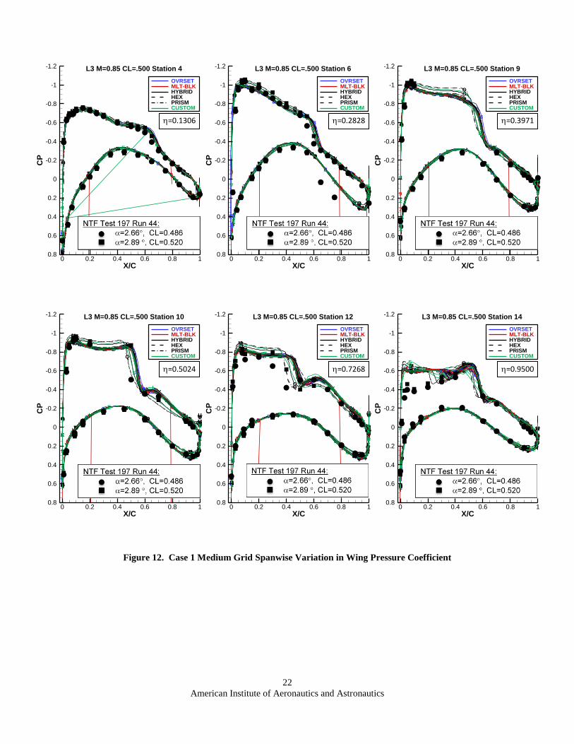
22

American Institute of Aeronautics and Astronautics

Figure 12. Case 1 Medium Grid Spanwise Variation in Wing Pressure Coefficient

B

B

B

B

BBBB

B

B

B

E

E

E

E

E

E

E

EE

E

EE

E

E

E

E

E

EEEEI

I

I

I

I

IJJ

J

J

J

JJ

J

J

JJ

K

K

K

KKK

K

K

K

K

K

L

L

L

L

MM

M

M

M

MNN

N

N

N

NOOO

O

O

O

O

O

O

OOPPP

P

P

P

P

P

P

P

PQQQ

Q

Q

Q

Q

Q

Q

QQRRR

R

R

R

R

R

R

R

RS

S

S

S

S

ST

T

T

T

T

TU

U

U

U

U

UVV

V

V

V

VWW

W

W

W

WXXX

X

X

X

X

X

X

X

X

Y

Y

Y

YY

Y

Z

ZZ

Z

Z

Z2

2

2

22

2

2

22

2

2

33

3

3

3

344

4

4

4

455

5

5

5

5666

6

6

6

6

6

6

6

677

7

7

778

8

8

8

8

9

9

9

9

9

9

aa a

a

a

a

bb

b

b

b

bdd

d

d

d

deee

e

e

e

e

e

e

e

efff

f

f

f

f

f

f

f

fgg

g

g

g

ghh

h

h

h

hkkk

k

k

k

k

k

k

kk

m

m

mm

m

m

n

n

nn

n

n

q

q

qq

q

q

r

r

rr

r

r

t

t

t

t

t

ts

s

s

s

sv

v

v

v

v

X/C

CP

0 0.2 0.4 0.6 0.8 1

-1.2

-1

-0.8

-0.6

-0.4

-0.2

0

0.2

0.4

0.6

0.8

L3 M=0.85 CL=.500 Station 4

OVRSETMLT-BLKHYBRIDHEXPRISMCUSTOM

B

B

B

B

BB

BB

BB

B

EE

E

EE

E

E

EE

E

EE

E

E

E

E

E

EEE

E

I

I

I

I II

JJ

J

J

J

J

J

J

JJ

JK

K

K

K

K

KK

KK

K

K

L

L

L

L

M

M

M

M

M

MN

N

N

N

N

NO

OO

O

O

O

O

O

O

OOP

PP

P

P

P

P

P

P

PPQ

QQ

Q

Q

Q

Q

Q

Q

QQR

RR

R

R

R

R

R

R

RR

S

S

S

S

ST

T

T

T

TU

U

U

U

U

UV

V

V

V

V

VW

W

W

W

W

WX

XX

X

X

X

X

X

X

XX

Y

Y

Y

Y

Y

Y

Z

Z

Z

Z

Z

Z

22

2

2

2

2

2

2

3

3

3

3

3

34

4

4

4

4

45

5

5

5

5

56

66

6

6

6

6

6

6

66

7

7

7

7 77

8

8

8

8

8

8

9

9

9

9

9

9

a

a

a

a

a

a

b

b

b

b

b

bd

d

d

d

d

de

ee

e

e

e

e

e

e

eef

ff

f

f

f

f

f

f

ffg

g

g

g

g

gh

h

h

h

h

hk

kk

k

k

k

k

k

k

kk

m

m

m

m

m

m

n

n

n

n

n

n

q

q

q

q

q

q

r

r

r

r

r

r

t

t

t

t tts

s

s

s

sv

v

v

v

v

X/C

CP

0 0.2 0.4 0.6 0.8 1

-1.2

-1

-0.8

-0.6

-0.4

-0.2

0

0.2

0.4

0.6

0.8

L3 M=0.85 CL=.500 Station 6

OVRSETMLT-BLKHYBRIDHEXPRISMCUSTOM

B

B

B

B

BB

B

B

BB

B

EE

E

EE

E

E

E

E

E

EE

E

E

E

E

EEEE

E

I

I

I

I

I

I

JJ

J

J

J

J

J

J

J J

JK

K

K

K

K

K

K

K

K

KK

L

L

L

L

M

M

M

M

M

MN

N

N

N

N

N

O

O

O

O

O

O

O

O

O

OOP

PP

P

P

P

P

P

P

PPQ

QQ

Q

Q

Q

Q

Q

Q

QQR

RR

R

R

R

R

R

R

RR

S

S

S

S

T

T

T

T

U

U

U

U

U

UV

V

V

V

V

VW

W

W

W

W

WX

XX

X

X

X

X

X

X

XX

Y

Y

Y

Y

Y

Y

Z

Z

Z

Z

Z

2

2

2

2

2

223

3

3

3

3

34

4

4

4

4

45

5

5

5

5

56

66

6

6

6

6

6

6

667

7

7

7

77

8

8

8

8

8

8

99

9

9

9

9

a

a

a

a

a

ab

b

b

b

b

bd

d

d

d

d

de

ee

e

e

e

e

e

e

eef

ff

f

f

f

f

f

f

ffg

g

g

g

g

gh

h

h

h

h

hk

kk

k

k

k

k

k

k

kk

m

m

m

m

m

m

n

n

n

n

n

n

q

q

q

q

q

q

r

r

r

r

r

r

t

t

t

t

t

ts

s

s

s

sv

v

v

v

v

X/C

CP

0 0.2 0.4 0.6 0.8 1

-1.2

-1

-0.8

-0.6

-0.4

-0.2

0

0.2

0.4

0.6

0.8

L3 M=0.85 CL=.500 Station 9

OVRSETMLT-BLKHYBRIDHEXPRISMCUSTOM

B

B

B

B

BB

B

B

B

B

B

EE

E

E

E

E

E

E

E

E

EE

E

E

E

E

EEEE

E

I

I

I

I

I

I

J

JJ

J

J

J

J

J

J

JJK

KK

K

KK

K

K

K

KK

L

L

L

L

M

M

M

M

MM

N

N

N

N

N

N

O

O

O

OO

O

OO

OOO

P

P

P

PP

P

PP

P

PP

Q

Q

Q

QQ

Q

Q

Q

QQQ

R

R

R

RR

R

RR

R

RR

S

S

S S

T

T

TT

U

U

U

U

U

U

V

V

V

V

V

V

W

W

W

W

W

WX

X

X

XX

X

XX

X

XX

Y Y

Y

Y

Y

Y

Z

Z

Z

Z

Z

2

2

2

2

2

2

2

3

3

3

3

3

34

4

4

4

4

45

5

5

5

5

56

6

6

66

6

66

6

66

7

7

7

7

7

7

8

8

8

8

8

8

99

9

9

9

9

a

a

a

a

a

ab

b

b

b

b

bd

d

d

d

d

de

e

e

ee

e

ee

e

eef

f

f

ff

f

ff

f

ffg

g

g

g

g

gh

h

h

h

h

hk

k

k

kk

k

kk

k

kk

m

m

m

m

m

m

n

n

n

n

n

n

q

q

q

q

q

q

r

r

r

r

r

r

t

t

t

t

t

ts

s

s

s

sv

v

v

v

v

X/C

CP

0 0.2 0.4 0.6 0.8 1

-1.2

-1

-0.8

-0.6

-0.4

-0.2

0

0.2

0.4

0.6

0.8

L3 M=0.85 CL=.500 Station 10

OVRSETMLT-BLKHYBRIDHEXPRISMCUSTOM

B

B

B

B

BB

B

B

B

B

BEE

E

EE

E

E

E

E

E

EE E

E

E

E

EEEE

E

I

I

I

I

I

I

JJ

J

J

J

J

J

J

J J

JKK

K

K

K

K

K

K

K

K

K

L

L

L

L

M

M

M

M

M

MN

N

N

N

N

NO

O

O

OO

O

O

O

O

OOP

P

P

PP

P

P

P

P

PPQ

Q

Q

QQ

Q

Q

Q

Q

QQR

R

R

RR

R

R

R

R

RRS

S

S

S

T

T

T

T

U

U

U

U

U

U

V

V

V

V

V

V

W

W

W

W

W

WX

X

X

XX

X

X

X

X

XX

Y

Y

Y

Y

Y

Y

Z

Z

Z

Z

Z

2

2

2

2

2

3

3

3

3

3

34

4

4

4

4

45

5

5

5

5

56

6

6

66

6

6

6

6

667

7

7

7

7

7

8

8

8

8

8

8

9

99

9

9

9

a

a

a

a

a

a

b

b

b

b

b

bd

d

d

d

d

de

e

e

ee

e

e

e

e

eef

f

f

ff

f

f

f

f

ffg

g

g

g

g

gh

h

h

h

h

hk

k

k

kk

k

k

k

k

kk

m

m

m

m

m

m

n

n

n

n

n

n

q

q

q

q

q

q

r

r

r

r

r

r

t

t

t

t

t

t

s

s

s

s

sv

v

v

v

v

X/C

CP

0 0.2 0.4 0.6 0.8 1

-1.2

-1

-0.8

-0.6

-0.4

-0.2

0

0.2

0.4

0.6

0.8

L3 M=0.85 CL=.500 Station 12

OVRSETMLT-BLKHYBRIDHEXPRISMCUSTOM

B

BB

B

BB

BB

B

B

B

EE

E

E

E

E

E

E

E

E E E

E E

E

E

EEEE

E

I

I

I

I

I

IJJ

J

J

J

J

J

J

J J

JK

KK

K

K

K

K K

K

KK

L

L

L

L

M

M

M

M

M

MN

N

N

N

N

NO

OO

OO

O

OO

O

OOP

PP

PP

P

PP

P

PPQ

QQ

QQ

Q

QQ

Q

QQR

RR

RR

R

RR

R

RRS

S

S

T

T

T

U

U

U

U

U

U

V

V

V

V

V

V

W

W

W

W

W

WX

XX

XX

X

XX

X

XX

Y

Y

Y

Y

Y

Y

Z

Z

Z

Z

Z

2

2

2

23

3

3

3

3

34

4

4

4

4

45

5

5

5

5

56

66

66

6

66

6

667

7

7

7

7

7

8

88

8

8

8

9

9

9

9

9

9

a

a

a

a

a

ab

b

b

b

b

bd

d

d

d

d

de

ee

ee

e

e e

e

eef

ff

ff

f

ff

f

ffg

g

g

g

g

gh

h

h

h

h

hk

kk

kk

k

k

k

k

kk

m

m

m

m

m

m

n

n

n

n

n

n

q

q

q

q

q

q

r

r

r

r

r

r

t

t

t

t

tts

s

s

s

sv

v

v

v

v

X/C

CP

0 0.2 0.4 0.6 0.8 1

-1.2

-1

-0.8

-0.6

-0.4

-0.2

0

0.2

0.4

0.6

0.8

L3 M=0.85 CL=.500 Station 14

OVRSETMLT-BLKHYBRIDHEXPRISMCUSTOM

=0.1306

=0.7268 =0.5024

=0.3971 =0.2828

=0.9500

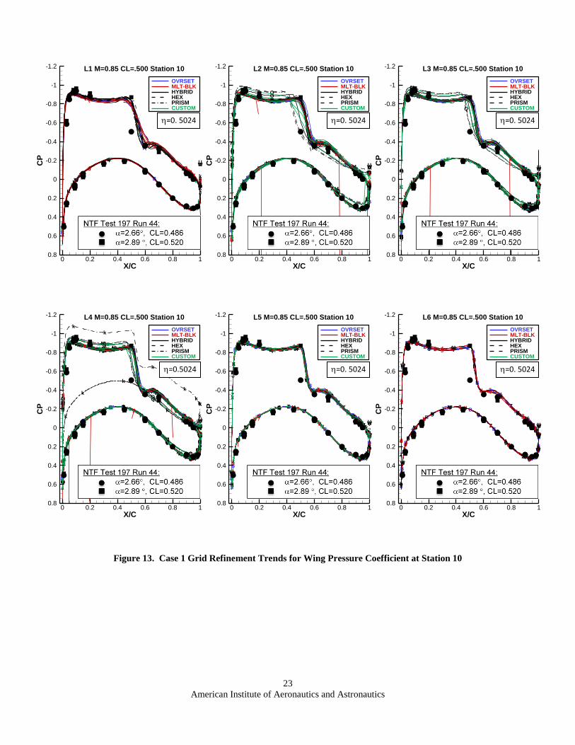
23

American Institute of Aeronautics and Astronautics

Figure 13. Case 1 Grid Refinement Trends for Wing Pressure Coefficient at Station 10

B

B

B

B

B

B

E

E

E

E

E

E

E

E

EE

E

I

I

I

J

J

J

J

J

JK

K

K

K

K

K

U

U

U

V

V

V

W

W

W

X

X

X

X

X

X

Y

Y

Y

Z

ZZ

33

3

44

4

a

aa

b

b

b

d

d

d

e

e

e

e

e

ef

f

f

f

f

f

k

k

k

k

k

k

m

m

m

q

q

q

r

r

r

t

t

X/C

CP

0 0.2 0.4 0.6 0.8 1

-1.2

-1

-0.8

-0.6

-0.4

-0.2

0

0.2

0.4

0.6

0.8

L1 M=0.85 CL=.500 Station 10

OVRSETMLT-BLKHYBRIDHEXPRISMCUSTOM

B

B

B

B

B

B

BB

E

E

EE

E

E

E

EE

E

E

EE

E

I

I

I

I

J

J

J

J

J

J

J

J

K

K

K

K

K

KK

K

L

L

L

M

M

M

M

N

N

N

NO

O

O

O

O

O

OO

P

P

P

P

P

P

P

P

Q

Q

Q

Q

Q

Q

QQ

R

R

R

R

R

R

R

R

S

S

S

T

T

T

U

U

U

UV

V

V

VW

W

W

W

X

X

X

X

X

X

X

XY

Y

Y

Y

ZZ

Z

Z22

2

3

3

33

4

4

4

4

5

5

5

5

6

6

6

66

6

6

67

7

7

7

8

88

8

8

89

9

9

9

a

a

a

a

b

b

b

b

bd

d

d

d

de

e

e

e

e

e

e

ef

f

f

f

f

f

f

fg

g

g

g

h

h

h

h

k

k

k

k

k

k

k

km

m

m

m

n

n

n

n

q

q

q

q

r

r

r

r

t

t

t

t

ss

s

vv

v

X/C

CP

0 0.2 0.4 0.6 0.8 1

-1.2

-1

-0.8

-0.6

-0.4

-0.2

0

0.2

0.4

0.6

0.8

L2 M=0.85 CL=.500 Station 10

OVRSETMLT-BLKHYBRIDHEXPRISMCUSTOM

B

B

B

B

BB

B

B

B

B

B

EE

E

E

E

E

E

E

E

E

EE

E

E

E

E

EEEE

E

I

I

I

I

I

I

J

JJ

J

J

J

J

J

J

JJK

KK

K

KK

K

K

K

KK

L

L

L

L

M

M

M

M

MM

N

N

N

N

N

N

O

O

O

OO

O

OO

OOO

P

P

P

PP

P

PP

P

PP

Q

Q

Q

QQ

Q

Q

Q

QQQ

R

R

R

RR

R

RR

R

RR

S

S

S S

T

T

TT

U

U

U

U

U

U

V

V

V

V

V

V

W

W

W

W

W

WX

X

X

XX

X

XX

X

XX

Y Y

Y

Y

Y

Y

Z

Z

Z

Z

Z

2

2

2

2

2

2

2

3

3

3

3

3

34

4

4

4

4

45

5

5

5

5

56

6

6

66

6

66

6

66

7

7

7

7

7

7

8

8

8

8

8

8

99

9

9

9

9

a

a

a

a

a

ab

b

b

b

b

bd

d

d

d

d

de

e

e

ee

e

ee

e

eef

f

f

ff

f

ff

f

ffg

g

g

g

g

gh

h

h

h

h

hk

k

k

kk

k

kk

k

kk

m

m

m

m

m

m

n

n

n

n

n

n

q

q

q

q

q

q

r

r

r

r

r

r

t

t

t

t

t

ts

s

s

s

sv

v

v

v

v

X/C

CP

0 0.2 0.4 0.6 0.8 1

-1.2

-1

-0.8

-0.6

-0.4

-0.2

0

0.2

0.4

0.6

0.8

L3 M=0.85 CL=.500 Station 10

OVRSETMLT-BLKHYBRIDHEXPRISMCUSTOM

B

BB

B

B

B

BB

BB

BB

B

B

B

B

EEE

E

E

EE

E

E

E

E

E

E

E

EE E

E EE

E

E

E

E

EEEEE

E

E

II

I

I

I

I

I I

JJJ

J

J

JJ

J

J

J

J

J

J J

J

JK

KK

K

KK

K

KK

K

K

K

K

K

K

K

L

L

L

L

L

L

M

M

M

M

M

M

MM

N

N

N

N

N

N

N

N

O

O

OO

O

O

O

O

O

O

O

O

OOOO

P

P

PP

P

P

P

P

P

P

P

P

P

PPP

Q

Q

QQ

Q

Q

Q

Q

Q

Q

Q

Q

QQQQ

R

R

RR

R

R

R

R

R

R

R

R

R

RRR

SS

S

S

S

T

T

T

T

T

U

U

UU

U

U

U

U

V

V

VV

V

V

V

V

W

W

WW

W

W

W

WX

X

XX

X

X

X

X

X

X

X

X

X

X

XX

Y

Y

YY

Y

YY

Y

Z

Z

Z

Z

Z2

2

2

2

2

2

22

2

3

3

3

3

3

3

3

34

4

4

4

4

4

4

45

5

5

5

5

5

5

56

6

66

6

6

6

6

6

6

6

6

6

6

667

7

7

77

7

7

7

8

8

8

8

8

8

9

9

9

9

9

9

9

9

9a

a

a

a

a

a

a

a

b

b

b

b

b

b

b

bd

d

d

d

d

d

d

de

e

ee

e

e

e

e

e

e

e

e

e

e

eef

f

ff

f

f

f

f

f

f

f

f

f

f

ffg

g

g

g

g

g

g

gh

h

h

h

h

h

h

h

k

k

kk

k

k

k

k

k

k

k

k

k

kkk

m

m

m m

m

m

m

m

n

n

n n

nn

n

n

q

q

q q

q

q

q

q

r

r

r r

rr

r

r

tt

t

t

t

t

t t

s

s

s

s

s

s

sv

v

v

v

v

v

v

X/C

CP

0 0.2 0.4 0.6 0.8 1

-1.2

-1

-0.8

-0.6

-0.4

-0.2

0

0.2

0.4

0.6

0.8

L4 M=0.85 CL=.500 Station 10

OVRSETMLT-BLKHYBRIDHEXPRISMCUSTOM

B

B

BB

B

B

B

BBBB

B

BB

BB

B

B

B

B

B

II

I

I

I

II

I

I I

I

L

L

L

L

L

L

L

U

UU

U

U

U

U

U

U

UU

V

VV

V

V

V

V

V

V

VV

W

WW

W

W

W

W

W

W

WWX

X

XXX

X

X

X

X

X

X

X

XX X

X

X

X

XXX

Y

Y

Y

Y

Y

Y

Y

Y

YY

Y

Z

Z

Z

Z

Z

ZZ

Z

Z

Z

Z

2

2

2

2

22

2

2

2

22

2

2

2

2

2

3

33

33

3

33

3

334

4

4

44

4

44

4

445

5

5

55

5

55

5

556

6

666

6

6

6

6

6

6

6

6

6 6

6

6

6

66677

7

7

7

7

7

7

7 7

7

8

88

8

8

8

8

8

9

9

9

9

9

9

9

9

99

9

a

a

a

a

a

a

aaa

a

a

b

b

b

bb

b

b

b

b

bbd

d

d

dd

d

d

d

d

ddf

f

fff

f

f

f

f

f

f

f

ff f

f

f

f

fffg

g

g

gg

g

gg

g

ggh

h

h

hh

h

hh

h

hh

m

m

m

m

m

m

mm

m

mm

n

n

n

n

n

n

nn

n

nn

q

q

q

q

q

q

qq

q

qq

r

r

r

r

r

r

rr

r

rr

tt

t

t

t

t

t

t

t t

ts

s

ss

s

s s

s

ssv

v

vv

v

v v

v

vv

X/C

CP

0 0.2 0.4 0.6 0.8 1

-1.2

-1

-0.8

-0.6

-0.4

-0.2

0

0.2

0.4

0.6

0.8

L5 M=0.85 CL=.500 Station 10

OVRSETMLT-BLKHYBRIDHEXPRISMCUSTOM

B

B

B BB B

B

B

B

BB

BBBBBB

BBB

BBB

B

B

BB

B

B

B

B

U

U

UU

U

U

U

U

U

UU

U

U

UUU

V

V

VV

V

V

V

V

V

VV

V

V

VVV

W

W

WW

W

W

W

W

W

WW

W

W

WWW

Z

Z Z

Z

Z

Z

Z

Z

Z3

3

33

3

3

3

3

3

3

3

3

3

3

334

4

44

4

4

4

4

4

4

4

4

4

444a

a

aa

a

a

a

aa

aa

a

a

aa

a

b

b

bb

b

b

b

bb

b

b

b

b

b

bbd

d

dd

d

d

d

dd

d

d

d

d

d

ddg

g

gg

g

g

g

gg

gg

g

g

gg

g

h

h

hh

h

h

h

hh

hh

h

h

hh

h

X/C

CP

0 0.2 0.4 0.6 0.8 1

-1.2

-1

-0.8

-0.6

-0.4

-0.2

0

0.2

0.4

0.6

0.8

L6 M=0.85 CL=.500 Station 10

OVRSETMLT-BLKHYBRIDHEXPRISMCUSTOM

=0. 5024 =0.5024 =0. 5024

=0. 5024 =0. 5024 =0. 5024

24

American Institute of Aeronautics and Astronautics

Figure 14. “Pseudo” Test Data

Figure 15. Lift and Pitching Moment for All Solutions

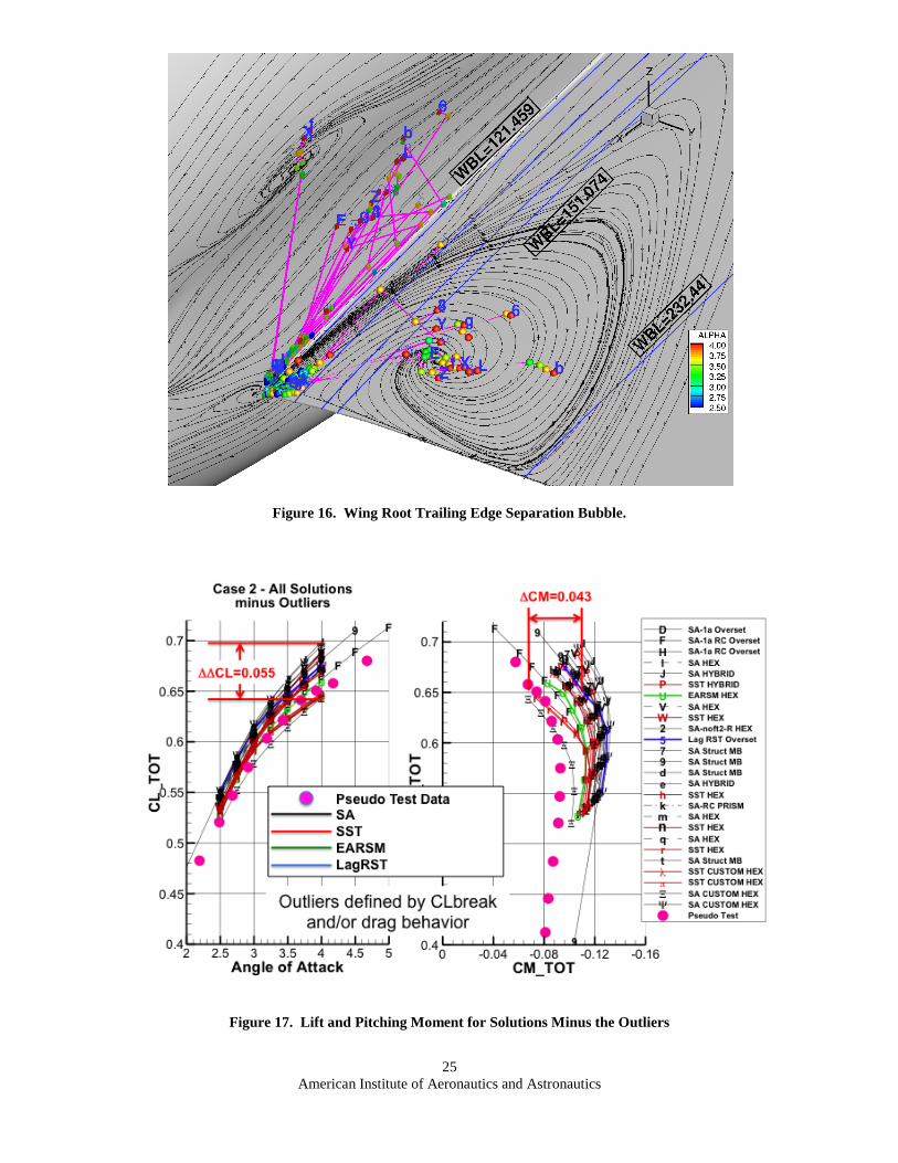
25

American Institute of Aeronautics and Astronautics

Figure 16. Wing Root Trailing Edge Separation Bubble.

Figure 17. Lift and Pitching Moment for Solutions Minus the Outliers

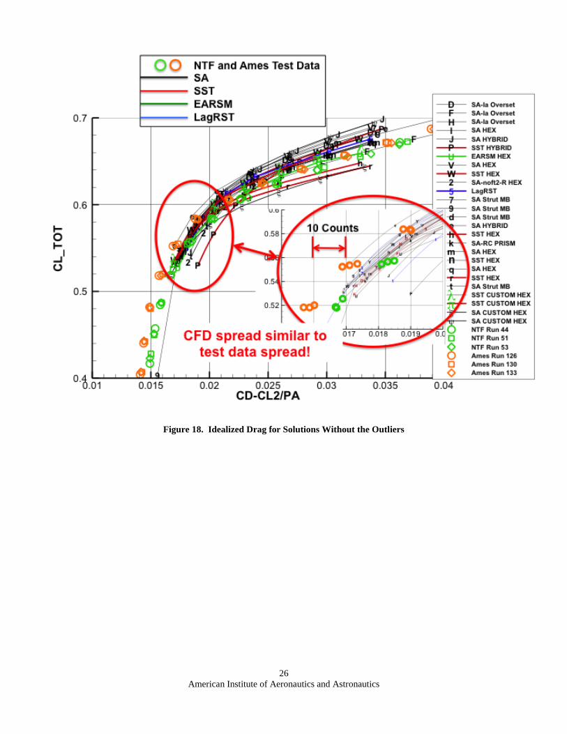
26

American Institute of Aeronautics and Astronautics

Figure 18. Idealized Drag for Solutions Without the Outliers

27

American Institute of Aeronautics and Astronautics

Figure 19. Case 2 Buffet Study Trends for Wing Pressure Coefficient at Station 10

I I I I I I I I I I I I I I I IJ J J J J J J J J J J J J J J J

M

M

M MM

M

MM

M

MM

M MM

M MN

N N N N N N N

N

NN

N N N

N

N

O

OO O

O

O

OO

O

OO

O OO

O O

P

P P P P P P P

P

P PP

P

P

P

P

Q

QQ Q

Q

Q

QQ

Q

QQ

Q QQ

Q Q

R

R R R R R R R

R

R R

R R

R

R

RS S S S

S

S

S S

S

SS

S SS

S ST T T T T T T T T

T

T T TT T TU U U U U U U U U U U U U U U UV V V V V V V V V

V

V V V V V VW W W W W W W W W

W

W W W W W WX X X X X X X X X X XX X X X XY Y Y Y Y Y Y Y Y

Y YY Y Y Y YZ Z Z Z Z Z Z Z Z

Z ZZ Z Z Z Z2 2 2 2 2 2 2 2 2 2 2 2 2 2 2 23 3 3 3 3 3 3 3 3

33 3 3 3 3 34 4 4 4 4 4 4 4 4

44

4 4 4 4 46

6 6 6 6 6 6 66 6 6 6 6 6 6 67 7 7 7 7 7 7 7

7

7 7 7 7 7 7 79

9 9 9 9 9 9 9 9

99

9 9 9 9 9

b

b

b

b

b b b b b b b b b b b bg g g g g g g g gg g

g g g g gh h h h h h h h h h h h h h h hk

k k k k k k

kk

k kk

k

k

k

km m m m m m m m m m m m m m m mq q q q q q q q q q q q q q q qr r r r r r r r r r

r

r r r r rt t t t t t t t t

t

t t t t t tX X X X X X X XX

X

X

X XX X Xz z z z z z z z z

z zz z z z zs s s s s s s s s

s s s s s s s

b

b b b b b b b b

b

b b b b b b

Section

Tra

ilin

gE

dg

eS

ep

ara

tio

n%

*10

0

1 2 3 4 5 6 7 8 9 10 11 12 13 14 15 160

0.1

0.2

0.3

0.4

0.5

0.6

0.7

0.8

0.9

1

RTSST

SAEARSM, RST

Overset, MB, Hyb., Cust.

Hex.

Prism

Trailing Edge Separation, Alpha = 3.0o

I I I I I I I I I I I I I I I IJ J J J J J J J J J J JJ

J J J

M

M

M M

M

M

MM

M

M

M

M

M

MM M

N

N N N N

N

N

N

N

N

NN

N

N

N

N

O

O

O O

O

O

O O

O

O

OO

O O

O

O

P

P P P P

PP

P

P

P

PP

P

P

P

P

Q

QQ Q

Q

Q

Q Q

Q

Q

Q

Q

Q

Q

Q

Q

R

R R R R

R

R

R

R

R

R RR

R

R

R

S

SS S

S

S

SS

S

S

S S

S

SS

S

TT T T T

T

T

TT

T

T T

TT T TU U U U U U U

UU

U

U

U U

U

U

UV V V V V V V

V

V

V V VV

V

V

VW W W W W W W

WW

W

W

W W

W

W

WX X X X X X X XX X

X

X

XX X XY Y Y Y Y Y Y Y Y Y Y Y Y Y Y YZ Z Z Z Z Z Z Z Z Z Z

Z

ZZ Z Z2 2 2 2 2 2 2 2 2 2 2 2 2 2 2 23 3 3 3 3 3 3 3 3 3 3 3

33 3 34 4 4 4 4 4 4 4 4 4 4

44 4 4 4

6

6

6

6

6 6 6 6

6

6

6

6

6

6 6 67 7 7 7 7 7 7 7 7

7

7

7

7 7 7 7

9

9 9 9 9 9

99

9

9

9

9

9

9

9

9

bb

b

b

b b b b b b b b b b

b

bg g g g g g g g g g g gg

g g gh h h h h h h h h h h h h h h h

k

k k k

kk

k

kk

k

kk

k k

k

k

m m m m m m m m m m m m m

m

m mq q q q q q q q q q q q q q

q

qr r r r r r r r

r

r r r r

r

r

r

t

t t t t t

t

t

t

t

t

t t

t

t

tX X X X X X X X X X X XX

X X Xz z z z z z z z z z z

z

zz z zs s s s s s s s s s s s

ss s s

bb

b

b

bb b b b b

bb b

b

b

b

Section

Tra

ilin

gE

dg

eS

ep

ara

tio

n%

*10

0

1 2 3 4 5 6 7 8 9 10 11 12 13 14 15 160

0.1

0.2

0.3

0.4

0.5

0.6

0.7

0.8

0.9

1

RTSST

SAEARSM, RST

Overset, MB, Hyb., Cust.

Hex.

Prism

Trailing Edge Separation, Alpha = 4.0o

Figure 20. Trailing Edge Separation at 3.0 and 4.0 Angle-of-Attack

E

E

EE

E

E

E

EE

E

E

EE

E

F

F

FF

F

F

F

FF

F

F

FF

F

I

I

I

I

I

I

J

JJ

J

J

J

J J

J

JJ

L

L

L

L M

M

M

M

MM

N

N

N

N

N

N

O

O

O

OO

O

O

O

OOOP

P

P

PP

P

PP

P

PP

Q

Q

Q

QQ

Q

Q

Q

QQQ

R

R

R

RR

R

RR

R

RRS

S

S S

T

T

T T

U

U

U

U

U

U

V

V

V

V

V

V

W

W

W

W

W

WX

X

X

XX

X

X X

X

XX

YY

Y

Y

Y

Y

Z

Z

Z

Z

Z

2

2

2

2

2

2

2

3

3

3

3

3

34

4

4

4

4

45

5

5

5

5

56

6

6

66

6

6 6

6

6677

7

7

7

7

8

8

8

8

8

8

99

9

9

9

9

a

a

a

a

a

ab

b

b

b

b

be

e

e

ee

e

e e

e

eef

f

f

ff

f

f f

f

ffg

g

g

g

g

gh

h

h

h

h

hk

k

k

kk

k

k k

k

kk

m

m

m

m

m

m

n

n

n

n

n

n

q

q

q

q

q

q

r

r

r

r

r

r

tt

t

t

t

t

b

b

b b

b

b

b

b

b

b

b

b

d

d

d d

d

d

d

d

dd

d

d

g

g

g g

g

g

g

g

gg

g

g

x

x

x

xx

x

x

x

x

xx

yy

yy

y

y

y

yy

y

y y

s

s

s

s

sv

v

v

v

v

X/C

CP

0 0.2 0.4 0.6 0.8 1

-1.2

-1

-0.8

-0.6

-0.4

-0.2

0

0.2

0.4

0.6

0.8

L3 M=0.85 ALPHA=2.75 Station 10

OVRSETMLT-BLKHYBRIDHEXPRISMCUSTOM

EE

EE

E

E

E

EE

E

E

EE

E

FF

FF

F

F

F

FF

F

F

FF

F

II

I

I

I

I

J

J

J

J

J

J

J J

J

JJ

L

L

L

LM

M

M

M

MM

N

N

N

N

N

NO

O

O

OO

O

O

O

O

OOP

P

P

PP

P

P P

P

PP

Q

Q

Q

QQ

Q

Q

Q

QQQ

R

R

R

RR

R

R R

R

RRS

S

SS

T

T

T T

U

U

U

U

UU

V

V

V

V

V

V

W

W

W

W

W

WX

X

X

XX

X

X X

X

XX

Y

Y

Y

Y

Y

Y

Z

Z

Z

Z

Z

2

2

2

2

2

2

2

3

3

3

3

3

34

4

4

4

4

45

5

5

5

5

56

6

6

66

6

6 6

6

6677

7

77

7

8

8

8

8

8

8

99

9

9

9

9

a

a

a

a

a

ab

b

b

b

b

be

e

e

ee

e

e e

e

eef

f

f

ff

f

f f

f

ffg

g

g

g

g

gh

h

h

h

h

hk

k

k

kk

k

k k

k

kk

m

m

m

m

m

m

n

n

n

n

n

n

q

q

q

q

q

q

r

r

r

r

r

r

tt

t

t

t

t

b

b

b b

b

b

b

b

b

b

b

b

d

d

d d

d

d

d

d

d

d

d

d

g

g

g g

g

g

g

g

g

g

g

g

x

x

x

xx

x

x

x

x

xx

yy

yy

y

y

y

yy

y

y y

s

s

s

s

sv

v

v

v

v

X/C

CP

0 0.2 0.4 0.6 0.8 1

-1.2

-1

-0.8

-0.6

-0.4

-0.2

0

0.2

0.4

0.6

0.8

L3 M=0.85 ALPHA=3.00 Station 10

OVRSETMLT-BLKHYBRIDHEXPRISMCUSTOM

EE

EE

E

E

E

EE

E

E

EE

E

FF

FF

F

F

F

FF

F

F

FF

F

II

I

I

I

I

J

J

J

J

J

J

J J

J

JJ

L

L

L

L

M

M

M

M

MMN

N

N

N

N

NO

O

O

O

O

O

O

O

O

OOP

P

P

PP

P

P P

P

PP

Q

Q

Q

Q

Q

Q

Q

Q

QQQR

R

R

RR

R

RR

R

RRS

S

S

S

T

T

TT

U

U

U

U

U

U

V

V

V

V

VV

W

W

W

W

WW

X

X

X

XX

X

X X

X

XX

Y

Y

Y

Y

Y

Y

Z

Z

Z

Z

Z

2

2

2

2

2

2

2

3

3

3

3

3

34

4

4

4

4

45

5

5

5

5

56

6

6

66

6

6 6

6

667

7

7 7 7

7

8

8

8

8

8

8

99

9

9

9

9

a

a

a

a

a

ab

b

b

b

b

be

e

e

ee

e

e e

e

ee

f

f

f

ff

f

f f

f

ff

g

g

g

g

g

gh

h

h

h

hhk

k

k

kk

k

k k

k

kk

m

m

m

m

m

m

n

n

n

n

n

n

q

q

q

q

q

q

r

r

r

r

r

r

tt

t

t

t

t

b

b

bb

b

b

b

b

bb

b

b

d

d

dd

d

d

d

d

dd

d

d

g

g

gg

g

g

g

g

gg

g

g

x

x

x

xx

x

x

x

x

xx

yy

yy

y

y

y

yy

y

y y

s

s

s

s

sv

v

v

v

v

X/C

CP

0 0.2 0.4 0.6 0.8 1

-1.2

-1

-0.8

-0.6

-0.4

-0.2

0

0.2

0.4

0.6

0.8

L3 M=0.85 ALPHA=3.25 Station 10

OVRSETMLT-BLKHYBRIDHEXPRISMCUSTOM

EE

EE

E

E

E

EE

E

E

EE

E

FF

FF

F

F

F

FF

F

F

FF

F

II

I

I

I

I

J

J

J

J

J

J

J J

J

JJ

L

L

L

L

M

M

M

M

MMN

N

N

N

N

NO

O

O

O

O

O

O

O

O

OOP

P

P

P

P

P

P P

P

PP

Q

Q

Q

Q

Q

Q

Q

Q

QQQR

R

R

R

R

R

R

R

R

RRS

S

S

S

T

T

T

T

U

U

U

U

U U

V

V

V

V

VV

W

W

W

W

WW

X

X

X

XX

X

X X

X

XX

Y

Y

Y

Y

Y

Y

Z

Z

Z

Z

Z2

2

2

2

2

2

23

3

3

3

3

34

4

4

4

4

45

5

5

5

5

56

6

6

6

6

6

6 6

6

66

77

77

7

7

8

8

8

8

8

8

9

9

9

9

9

9

a

a

a

a

a

ab

b

b

b

b

b

e

e

e

e

e

e

e e

e

ee

f

f

f

ff

f

f f

f

ff

g

g

g

g

g

gh

h

h

h

hhk

k

k

k

k

k

k k

k

kk

m

m

m

m

m

m

n

nn

n

n

n

q

qq

q

q

q

r

rr

r

r

r

tt

t

t

t

t

b

b

bb

b

b

b

b

b

b

b

b

d

d

dd

d

d

d

d

d

d

d

d

g

g

gg

g

g

g

g

g

g

g

g

x

x

x

xx

x

x

x

x

x xyy

yy

y

y

y

yy

y

y y

s

ss

s

sv

vv

v

v

X/C

CP

0 0.2 0.4 0.6 0.8 1

-1.2

-1

-0.8

-0.6

-0.4

-0.2

0

0.2

0.4

0.6

0.8

L3 M=0.85 ALPHA=3.50 Station 10

OVRSETMLT-BLKHYBRIDHEXPRISMCUSTOM

EE

EE

E

E

E

EE

E

E

EE

E

FF

FF

F

F

F

FF

F

F

FF

F

II

I

I

I

I

J

J

J

J

J

J

J

J

J

JJ

L

L

L

L

M

M

M

M

MMN

N

N

N

N

NO

O

O

O

O

O

O

O

O

OOP

P

P

P

P

P

PP

P

PP

Q

Q

Q

Q

Q

Q

Q

Q

QQQR

R

R

R

R

R

R

R

RRRS

S

S

S

T

T

T

T

U

U

U

U

U U

V

V

V

V

VV

W

W

W

W

WW

X

X

X

XX

X

X X

X

XX

Y

Y

Y

Y

Y

Y

Z

Z

Z

Z

Z2

2

2

2

2

2

2 3

3

3

3

3

34

4

4

4

4

4

5

5

5

5

5

5

6

6

6

6

6

6

6 6

6

66

77

7

7

7

7

8

8

8

8

8

8

9

9

9

9

9

9

a

a

a

a

a

a

b

b

b

b

b

b

e

e

e

e

e

e

e e

e

ee

f

f

f

ff

f

f f

f

ff

g

g

g

g

g

gk

k

k

k

k

k

kk

k

kk

m

mm

m

m

m

n

nn

n

n

n

q

qq

q

q

q

r

rr

r

r

r

tt

t

t

t

t

d

d

dd

d

d

d

d

d

d

d

d

g

g

gg

g

g

g

g

g

g

g

g

x

x

x

xx

x

x

x

x

x xyy

yy

y

y

y

y

y

y

y y

s

ss

s

sv

vv

v

v

X/C

CP

0 0.2 0.4 0.6 0.8 1

-1.2

-1

-0.8

-0.6

-0.4

-0.2

0

0.2

0.4

0.6

0.8

L3 M=0.85 ALPHA=3.75 Station 10

OVRSETMLT-BLKHYBRIDHEXPRISMCUSTOM

EE

EE

E

E

E

EE

E

E

EE

E

FF

FF

F

F

F

FF

F

F

FF

F

II

I

II

I

J

J

J

J

J

J

J

J

J

JJ

M

M

M

M

MMN

N

N

N

N

NO

O

O

O

O

O

O

O

O

OOP

P

P

P

P

P

P

P

P

PP

Q

Q

Q

Q

Q

Q

Q

Q

QQQR

R

R

R

R

R

R

R

R

RRS

S

S

S

T

T

T

T

U

U

U

U

U U

V

V

V

V

VV

W

W

W

W

WW

X

X

X

X

X

X

X X

X

XX

Y

Y

Y

Y

Y

Y

Z

Z

Z

Z

Z2

2

2

2

2

2

23

3

3

3

3

34

4

4

4

4

45

5

5

5

55

6

6

6

6

6

6

6 6

6

66

77

7

7

7

7

8

8

8

8

8

8

9

9

9

9

9

9

a

a

a

a

a

a

b

b

b

b

b

b

e

e

e

e

e

e

e e

e

e

e

f

f

f

f

f

f

f f

f

ff

g

g

g

g

g

g

h

h

h

h

h hk

k

k

k

k

k

k

k

k

kk

m

mm

m

m

m

n

n n

n

n

n

q

q q

q

q

q

r

r r

r

r

r

tt

t

tt

t

b

b

bb

b

b

b

b

b

b

b

b

d

d

d

d

d

d

d

d

d

d

d

d

g

g

gg

g

g

g

g

g

g

g

g

x

x

x

xx

x

x

x

x

x x

yyy

y

y

y

y

y

y

y

yy

s

ss

s

sv

vv

v

v

X/C

CP

0 0.2 0.4 0.6 0.8 1

-1.2

-1

-0.8

-0.6

-0.4

-0.2

0

0.2

0.4

0.6

0.8

L3 M=0.85 ALPHA=4.00 Station 10

OVRSETMLT-BLKHYBRIDHEXPRISMCUSTOM

=0. 5024 =0.5024 =0. 5024

=0. 5024 =0. 5024 =0. 5024

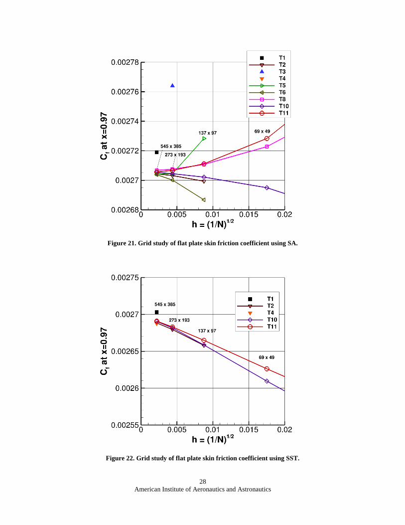
28

American Institute of Aeronautics and Astronautics

Figure 21. Grid study of flat plate skin friction coefficient using SA.

Figure 22. Grid study of flat plate skin friction coefficient using SST.

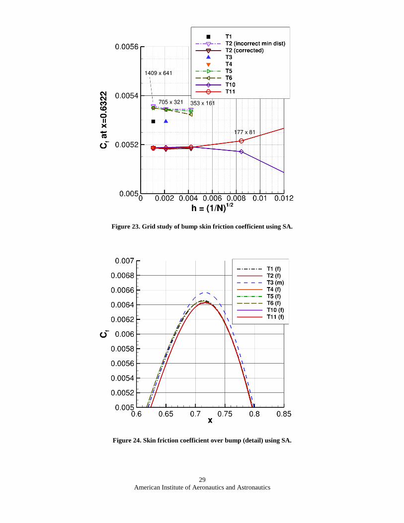
29

American Institute of Aeronautics and Astronautics

Figure 23. Grid study of bump skin friction coefficient using SA.

Figure 24. Skin friction coefficient over bump (detail) using SA.

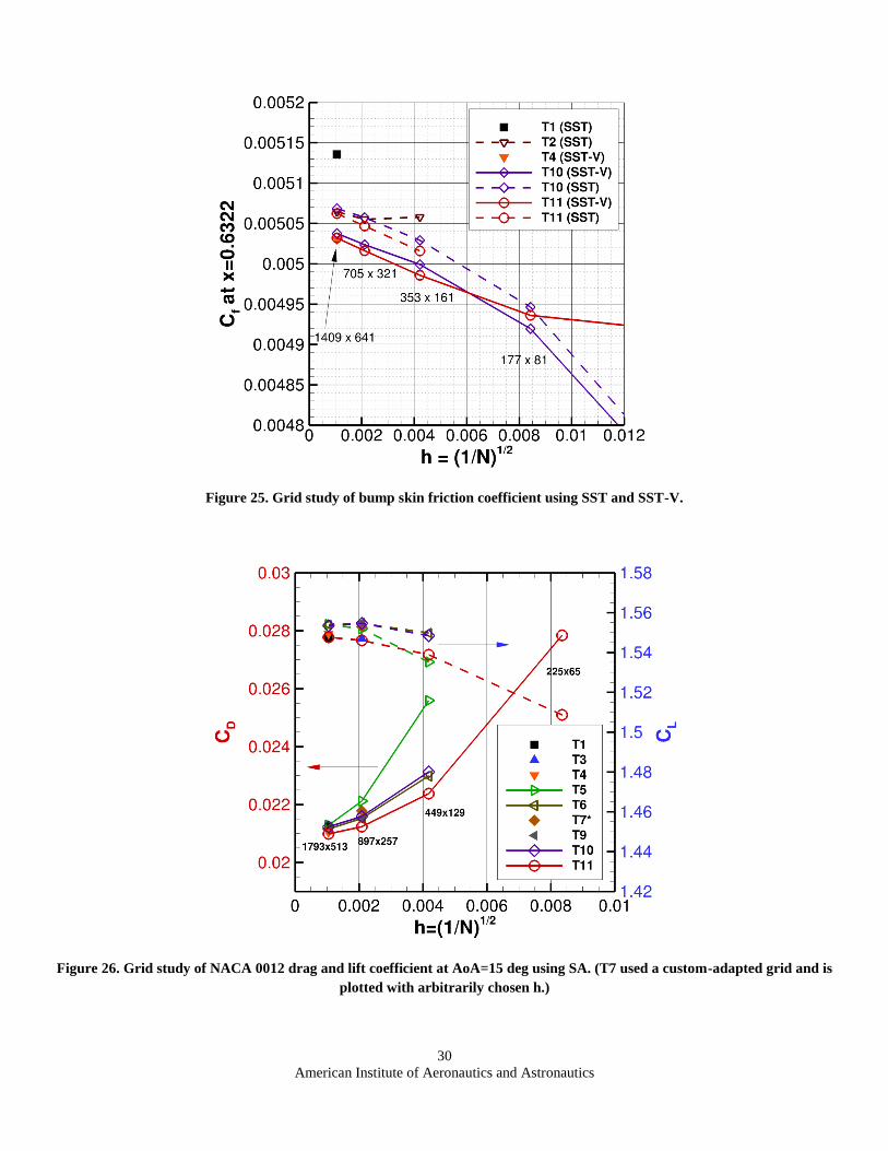
30

American Institute of Aeronautics and Astronautics

Figure 25. Grid study of bump skin friction coefficient using SST and SST-V.

Figure 26. Grid study of NACA 0012 drag and lift coefficient at AoA=15 deg using SA. (T7 used a custom-adapted grid and is

plotted with arbitrarily chosen h.)

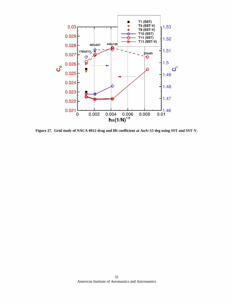
31

American Institute of Aeronautics and Astronautics

Figure 27. Grid study of NACA 0012 drag and lift coefficient at AoA=15 deg using SST and SST-V.