summation by parts, projections, and stability. i · summation by parts, projections, and...

mathematics of computationvolume 64, number 211july 1995, pages 1035-1065

SUMMATION BY PARTS, PROJECTIONS, AND STABILITY. I

PELLE OLSSON

Abstract. We have derived stability results for high-order finite difference ap-

proximations of mixed hyperbolic-parabolic initial-boundary value problems

(IBVP). The results are obtained using summation by parts and a new way

of representing general linear boundary conditions as an orthogonal projection.

By rearranging the analytic equations slightly, we can prove strict stability for

hyperbolic-parabolic IBVP. Furthermore, we generalize our technique so as to

yield stability on nonsmooth domains in two space dimensions. Using the same

procedure, one can prove stability in higher dimensions as well.

1. Introduction

When solving a partial differential equation numerically it is necessary to

have some bound of the growth rate of the solution, since otherwise roundoff

errors could grow arbitrarily fast. This upper bound can be established by ensur-

ing some kind of stability. We have elected to use the energy method, because

it can be applied to the continuous as well as the discrete model. Furthermore,

it can be applied to general domains, which is important when studying multi-

dimensional problems.Stability of the continuous problem is established by means of an integration-

by-parts procedure introducing boundary terms, some of which must be elimi-

nated to ensure stability. For the finite difference model integration by parts is

replaced by summation by parts. This amounts to designing the discrete differ-

ence operator ensuring that, in addition to the accuracy requirements, certain

conditions of antisymmetry are met. As a consequence, the common problemof finding proper "numerical" boundary conditions will be eliminated; they will

be built in the discrete difference operator.

The analytic boundary conditions are yet to be incorporated. We propose a

certain projection operator, which interacts with the difference operator so as

to generate boundary terms that are completely analogous to those of the con-

tinuous problem. This can be done for any type of linear boundary conditions.

Thus, an energy estimate is obtained for the discrete problem, provided there

is one for the analytic model. This conclusion remains true for domains in sev-

eral space dimensions, even if the boundary is nonsmooth. Furthermore, using

this projection operator allows us to derive stability results for a larger class offinite difference operators than those considered in [5]. Stability will be proved

Received by the editor January 19, 1994 and, in revised form, August 5, 1994.

1991 Mathematics Subject Classification. Primary 65M06, 65M12.This work has been sponsored by NASA under contract No. NAS 2-13721.

©1995 American Mathematical Society

1035

License or copyright restrictions may apply to redistribution; see https://www.ams.org/journal-terms-of-use

1036 PELLE OLSSON

• 1

uvdx

for high-order finite difference approximations of mixed hyperbolic-parabolic

variable-coefficient systems subject to general boundary conditions.

1.1. An introductory example. To illustrate the underlying principles of the en-

ergy method, we consider the convection-diffusion equation

Ui = uxx + ux, x 6 (0, 1) , í >0 ,

u(x,0) = f(x),w(0,o = o,ux(l, t) = g(t).

In the sequel we shall use the standard L2-scalar product

(u, v) =Jo

with the corresponding norm defined as ||u||2 = (u, u).

We can obtain an a priori estimate for this example using the following tools.

(i) Integration by parts:

^||«||2 = 2(u, uxx) + 2(u, ux) = -2\\ux\\2 + 2(u, ux) + 2uux\x0.

(ii) Boundary conditions:

^||M||2 = -2\\ux\\2 + 2(u, ux) + 2u(l, t)g(l, t).

(iii) Cauchy-Schwarz inequality:

^||w||2 < -2\\ux\\2 + 2\\u\\\\ux\\ + 2u(l, t)g(l, t).

(iv) Algebraic inequality:

2\xy\ < ex2 + e~xy2

implies ( e = 1 )

^IMI2<-||"*ll2 + IMI2 + "(i,02 + ar(i,02-

(v) Sobolev inequality:

\u\200<e\\ux\\2 + (e-x + \)\\u\\2

is used to eliminate u(\, t) ( e = 1)

^ll"ll2<3|MI2 + g(i,02,

which can be solved analytically to yield

\\u(-,t)\\2<e"(\\f\\2 + j\(r)2dr^ .

If we are to obtain such an estimate for a system of equations we will also need

(vi) The adjoint of A :

(u, Av) = (A1 u, <;).


SUMMATION BY PARTS, PROJECTIONS, AND STABILITY. I 1037

Summing up, the energy method boils down to the six basic "tools" above. In

the subsequent sections we shall see how these principles can be modified so as

to give an energy estimate for the semidiscrete system.

2. General principles for the semidiscrete case

In this section the basic principles of the energy method will be transferred to

the semidiscrete case. Furthermore, a number of lemmas, which will be needed

later, will be stated. Throughout this section grid vectors will be denoted by

vT = (v?... vT), Vj £ Rd . Difference operators approximating d/dx will be

designated by

/dool ... d0vI\

\d„oI • • • dvvI)

where D is written as a square matrix for convenience; in reality D will be a

banded matrix, where the bandwidth is independent of the mesh size h = 1/v .

2.1. Summation by parts. In the semidiscrete case we employ summation by

parts instead of integration by parts. The basic idea is to use difference operators

satisfying

(2.1) (u, Dv)h = uTvl/-uTv0-(Du,v)h

with respect to a weighted scalar product

V

(u,v)h = hJ2 Oijufvj.ij=0

It should be remarked that the usual Euclidean scalar product cannot be used.

To prove the existence of summation by parts, it suffices to consider scalar

products of the form

/Id) \(2.2) i= ; , x<" e R<"+')«/*(r,+i)rf > i = iy2,

V Wwhere the blocks of I are given by I,7 = o¡¡T, I e Rdxd ; r¡ and the elements

of I(/), / = 1, 2, are independent of h . The following existence proof can be

found in [5].

Proposition 2.1. There exist scalar products (2.2) and difference operators D of

accuracy 2p - 1 at the boundaries and 2p in the interior, p > 0, such that the

summation-by-parts property (2.1) holds.

Confining ourselves to the case where Z(1) and S(2) are diagonal, we have

the following existence theorem [4].

Proposition 2.2. There exist diagonal scalar products (2.2) and difference opera-

tors D of accuracy p at the boundaries and 2p in the interior, 1 < p < 4, such

that the summation-by-parts property (2.1) holds.


1038 PELLE OLSSON

Remark 2.0. If one omits the requirement that the boundary stencils be at least

accurate of order p for a given interior accuracy 2p, it is possible to prove

summation by parts for diagonal scalar products and difference operators D of

arbitrary order of accuracy [8]. For a given boundary accuracy p, however, it

may be necessary to resort to interior stencils of accuracy q » 2p, which may

render these operators useless in practice.

The actual computation of the operators above is ill-conditioned, since it

involves the solution of a rank-deficient problem. Using a symbolic language,

one can solve for D exactly, the elements of which in general will depend on

one or more parameters. Explicit examples can be found in [6]. For details on

the algorithms we refer to [9]. The simplest example is furnished by

/0.5 \1

'•.

1

V 0.5;Summation by parts can be generalized to several space dimensions if we

restrict ourselves to diagonal norms. To simplify the notation, we consider only

the two-dimensional case. A general proof is given in [6]. The grid function m,;

is partitioned as uT = (uT...«£), uj = (uL ...uTA , j - 0, ... ,v2. Define

the weighted scalar product as

1/, V2

(2.4) (u,v)h = h^2Ylaia)ulvij >;=0 7=0

where h — hxh2 is the cell area. Let Dx and D2 denote the difference operators

approximating d/dxx and d/dx2 . Define

(2.5) (Dxu)u = yJ2dikUkJ ' (D2u)u = ylHdikU* '1 fe=o 2 k=0

where it is assumed that the rr's and if s satisfy (2.1). Hence

(u, Dxv)h = A2 J ff; ( S CT/Mí ZIdikVkJj=0 V ¡=0 k=0

and a similar expression holds for (u, D2v)h . The parenthetical expression

satisfies (2.1) for each j . We thus arrive at

Proposition 2.3. Let the discrete difference operators Dx and D2 be defined by

(2.5). Summation by parts then holds in both dimensions,

v2 v2

(u,Dxv)h = fa^OjuljVvj - h2J2ojuZjV0j -(Dxu, v)h ,;=0 j=0

(u, D2v)h = hx^2 o-iuJV2vlVl -hx^2 GíuJqVm - (D2u ,v)h,(=0 ¡=o

(2.3)

D

( -1 1-0.5 0 0.5

-0.5 0 0.5

-1 1 /

where (•, -)h is defined by (2.4).



Remark 2.1. This is the discrete counterpart of the two-dimensional divergence

theorem. With a general domain Si we assume that there is a smooth map

¿; = Ç(x) taking Si onto the unit cube where Proposition 2.3 can be applied.

The assumption of such a map £ is necessary in order for finite difference

methods to apply to curvilinear domains. Consequently, integration by parts

can always be replaced with summation by parts in the discrete case. It is

presently unknown if it is possible to obtain the summation-by-parts property

in more than one dimension using nondiagonal norms.

2.2. Projections. Suppose that the model equation of §1.1 were discretized as

(2.6) vt = D2v + Dv,v ' v(0) = f,

where we have assumed homogeneous Neumann data for convenience; in Part

II [7] it will be shown how to treat inhomogeneous boundary conditions. For

every fixed h the problem above is a constant-coefficient ODE system with a

unique analytic solution. Consequently, there is little hope that the discretized

boundary conditions vo(t) = (Dv)v(t) = 0 are fulfilled, since they have not

been accounted for so far.

Denote by V c R"+1 the vector space where v$(t) - (Dv)v(t) — 0, and let

P be a projection of v onto V . Multiplying (2.6) by P yields

(Pv), = P (D2v + Dv\ .

Any solution of (2.6) satisfying the boundary conditions must obey v = Pv,

whence

(2.7) vt = P (D2v + Dv) .

Conversely, we have

Proposition 2.4. Let P G Rsxs be a given projection independent of t, and sup-

pose that v(t) G Rs is a solution of the nonlinear ODE system

(28) v, = PR(t,v) + (I-P)gt,v(0) = f ,

where f satisfies f = Pf+(I- P)g(0). Then

v(t) = Pv(t) + (I-P)g(t), t>0.

Proof. Since P is independent of /, premultiplication of (2.8) gives (P2 — P)

(Pv), = PR(t,v).

Using this equality in (2.8) implies

v, = (Pv + (I - P)g),.

Hence, by integration,

(I - p)(v(t) - g(t)) = (i - P)(f - g(0)),

which proves the proposition. □


1040 PELLE OLSSON

Remark 2.2. The function g(t) represents the boundary data, and (I - P) •

(v - g) = 0 is the extension of (/ - P)v = 0 to inhomogeneous boundary data.

Proposition 2.4 thus tells us that any solution to (2.8) will satisfy the boundary

conditions if the initial data do.

In general, P is not uniquely defined. Consider the vector space V = {v g

Rv+l\v0 = 0,vu=vv-l}. Then

¿> =

/o

V

\

o)

p =

/o

V

\

0 1

1/

both imply Pv g V. To shed some light on how to choose P, we apply the

energy method to (2.7):

d_dti-t\\v\\2h = 2(v,P(D2v + Dv))h.

If P were selfadjoint with respect to (•, •)„ , then

ddt

\v\\2h = 2(Pv , D2v + Dv)h = 2(v , D2v + Dv)h

where the last equality follows from Proposition 2.4. The crucial condition to

obtain this equality is expressed by

(2.9) (u,Pv)h = (Pu,v)h ,

which states that P is an orthogonal projection (using the weighted scalar prod-

uct (•, -)h).

Suppose that u(x, t) GRd, x e R" , is a solution to

ut = F(x, t, d)u , x G Si ,L(x, d)u = 0 , x G T ,

where d denotes the «-dimensional gradient; Y is the boundary of Si. This

system is discretized in space, possibly requiring a coordinate mapping onto theunit cube,

vt = PG(t, D)v .

The projection P should be such that v fulfills

LTv = 0 ,

where L now represents a discretization of the analytic boundary conditions.

Let V = {v e Rm\LTv = 0}. According to the preceding discussion, P is taken

to be the orthogonal projection onto V (with respect to (•, -)n). The boundaryconditions can be written as

QTZv - 0,

where Q = YrxL. Hence, the boundary conditions are fulfilled for all vectors

v that are orthogonal to the column space of Q, the orthogonal projection onto

which reads Q(QTZQ)~XQT2Z. In case 1 = 7, this is the standard projection.



The desired boundary projection is thus given by

P = I-Q(QT2ZQ)-XQT2Z,

or

(2.10) P = I-1-XL(LTI.-XL)-XLT.

Remark 2.3. In order for the projection to be well defined, the inverse of

LTYrxL must exist, which follows if and only if L has full column rank.

The latter will follow from assumptions on the analytic boundary conditions

(consistency arguments).

Proposition 2.5. Suppose that L has full column rank, and let P be defined by

(2.10). Then

(i) P2 = P,

(ii) ZP = PTI,,(iii) v = Pv <=> LTv = 0.

Proof. All statements are immediate consequences of (2.10). D

Remark 2.4. The second statement of Proposition 2.5 is equivalent to (2.9).

2.3. Some technical lemmas. In this subsection we have gathered some technical

results that will be needed in the subsequent presentation. Their proofs have

been deferred to the Supplement. As seen in §1.1, it is necessary to have a

Sobolev inequality. The following proposition shows that there is a discrete

Sobolev inequality for the norms that we are interested in. We present it in a

form suitable for proving strict stability.

Proposition 2.6. Let || • \\n and D be defined by (2.2) and (2.1), respectively.

Then|v|2X)<e||JDi;||2 + (e-1 + l+^(«))||t;|

2A '

where e > 0.

Let

(2.11)

¡A*A Aj = A(jh) , j = 0, ... , v , hv = 1 ,

Aj

,dxddenote the grid matrix representation of A(x¡) g R , x¡■ = hj e [0, 1].

Smoothness will be assumed as needed.

Lemma 2.1. Let I and A be defined by (2.2) and (2.11), respectively. Then

\(u,Av)h-(ATu,v)h\<cf(h)\\u\\h\\v\\h.

Remark 2.5. According to Lemma 2.1, the transpose of A is an approximate

adjoint with respect to (•, •)/, ; the perturbation consists of lower-order terms.

The following assumption will be crucial when proving strict stability for

hyperbolic systems.


1042 PELLE OLSSON

Assumption 2.1. Let A and X be given by (2.11) and (2.2). Then one of theconditions below is assumed to hold:

(i) X is diagonal diag(ero^ • • • OvI) ',

(ii) The blocks of A satisfy Aq = ■■• = Ar¡ and A„-fl — ■■ ■ = Av , where rx

and r2, rx > 0, 0 < r2 < v - rx , are defined by equation (2.2).

Corollary 2.1. If Assumption 2.1 holds, then (u, Av)„ = (ATu, v)„ .

Proof. In both cases, X and A commute. The corollary follows immedi-

ately. □

Remark 2.6. The latter criterion is satisfied if there is a ô > 0 such that A(x) =const for 0 < x < ô and 1 - ô < x < 1, and if h is chosen such that hr <5 ,

where r = max(rj, r2).

Lemma 2.2. Let X and A be defined by (2.2) and (2.11). Then

\(u,Av)h\<\A\(X(l+cf(h))\\u\\h\\v\\h,

where \A\oo = sup \A(x)\.

Corollary 2.2. If, in addition to the hypotheses of Lemma 2.2, Assumption 2.1 is

fulfilled, then\(u, Av)h\ < lAl^WuWhWvWh .

Remark 2.7. Lemma 2.2 states that the growth rate induced by low-order terms

is the same (modulo cf(tf)-terms) in the continuous and the semidiscrete case.

Denote by [D, A] the commutator of D and A. It is well known that

(u, [D, A]v)„ <\\[D, A]\\h\\u\\h\\v\\h , where \\[D, A]\\n can be bounded inde-pendently of h . This result can be sharpened under certain circumstances.

Lemma 2.3. Let D be a difference approximation satisfying the summation-by-

parts rule (2.1) with respect to a weighted norm (2.2), and define A by (2.11).

Suppose that Assumption 2.1 holds. If A is symmetric, then

(k,[D,^]ü)a</,([D,^])||«||ä||u||a,

where p([D, A]) is the spectral radius of [D, A], i.e., p([D, A]) = sup \Xk \, Xkan eigenvalue of [D, A].

3. One-dimensional problems

We shall successively consider hyperbolic, parabolic and mixed hyperbolic-

parabolic systems. Variable-coefficient matrices will be allowed. To simplify

the presentation, we shall only deal with the lower boundary x = 0, which is

justified if we take the solution to have compact support. In general, the upper

boundary x = 1 is treated in a fashion similar to the procedure at the lower

boundary.

3.1. Hyperbolic systems. Consider the hyperbolic system

(3.1)u, = Aux + Bu + F, jte(O.l), . xu(x,0) = f(x), A(x,t)=(A-{X'n ,

u.(0,t) = Lu+(0,t), LgR'1**, V A+(X>0J



where u eRd , dx + d2 = d ; A_ , A+ is the partitioning of A into negative

and positive eigenvalues. It is assumed that the elements of the diagonal matrix

A never change sign at the boundaries x = 0 and x = 1, and that there is

a constant y > 0 such that A-(j, t) < -y and A+(j, t) > y, j = 0, 1 .This implies that the rank of L is constant. Furthermore, L is assumed to be

"small".The discrete boundary conditions are written as LTv = 0, where

(3.2) LT=(LT 0 ... 0)eRd,x{l/+i)d.

Here, LT = (I -L) g RdlXd , the latter L being the analytic boundary oper-

ator. It follows immediately that rank(L) = rank(Z) = dx . The hypothesis of

Proposition 2.5 is thus satisfied, and we have the semidiscrete system

(3.3) vt = P(ADv + Bv + F),v ; v(0) = f,

/A(0,0

V A(1,0

Proposition 3.1. Let (•, •)* be given by (2.2) and suppose that D satisfies the

conclusion of Proposition 2.1. If P is defined by (2.10) and (3.2), then thesolution of (3.3) satisfies an energy estimate

\\v(t)\\l + f (lô(T)|2 + Mt)|2) dx < Ke("'+^)' (||/||2 + ¡' \\F(x)\\2d:

Proof. The energy method yields (using Propositions 2.5, 2.4)

^-t\\v\\2h = 2(v , t;,)* = 2(v , P(ADv + Bv + F))h

= 2(v , ADv)h + 2(v , Bv)h + 2(v , F)h .

Summation by parts implies (vv = 0)

(v, ADv)h = -VjfArjVo- (Dv, Av)„ - (v, [D, A]v)h.

Hence, by Lemma 2.1,

(v , ADv)h < -l^vTA0Vo + \ (K0\\v\\h\\hDv\\h + \\[D, A]\\h\\v\\2) ,

where hD is a bounded operator, i.e.,

(v , ADv)h < -Âoô + i (Kx + \\[D, A]||A) \\v\\2.

Now, according to Propositions 2.4, 2.5 we have LTv = 0, which is equivalent

to V- = Lv+ (the latter L denoting the analytic boundary operator). Thus,

v?A0v0 = vlA-V- + vlA+v+ = vi (A+ + LrA_L) v+ > -\v0\2 ,

where the last inequality follows from the boundary conditions and the assump-

tions on L and A. Note that the analytic problem would result in exactly the


1044 PELLE OLSSON

same inequality. Hence,

(t;, ADv)h < -]\v0\2 + \(KX + \\[D, A]\\n) \\v\\2

Lemma 2.2 shows that

(w,£t;)A<(|£U+ *(*)) ||«|ß.

Consequently,

i< [[(\\[D, A]|U + 2|5|oc + 1 + Kx+cf(h))\\v\\2 + \\F\\2)

min(l, y/2)

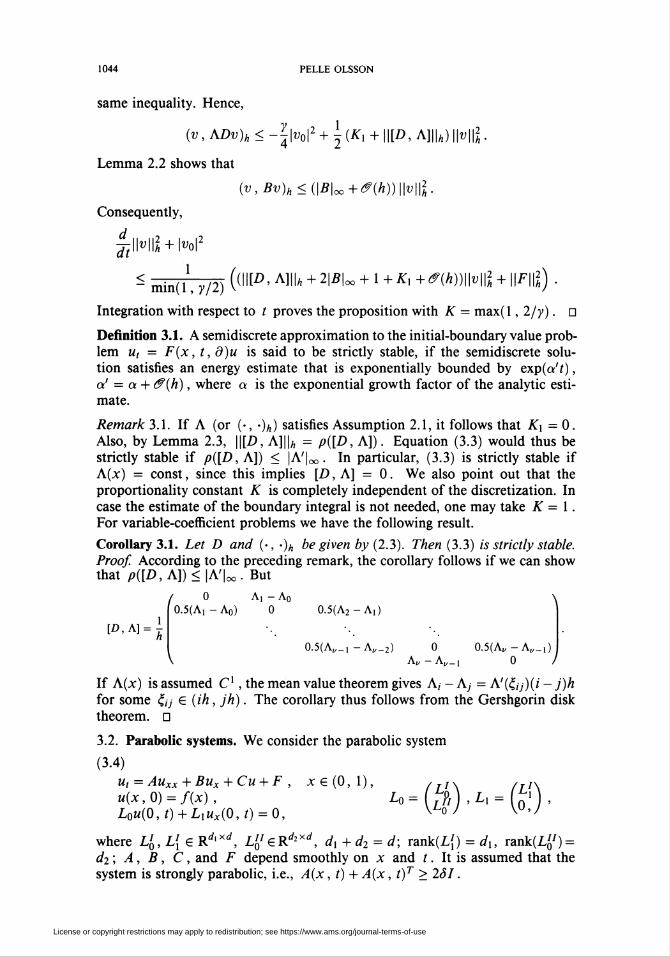
Integration with respect to t proves the proposition with K = max( 1, 2/y). D

Definition 3.1. A semidiscrete approximation to the initial-boundary value prob-

lem ut — F(x, t,d)u is said to be strictly stable, if the semidiscrete solu-tion satisfies an energy estimate that is exponentially bounded by exp(a'i),

a' = a + cf(h), where a is the exponential growth factor of the analytic esti-

mate.

Remark 3.1. If A (or (•, -)n) satisfies Assumption 2.1, it follows that Kx - 0.

Also, by Lemma 2.3, ||[Z>, A]\\„ = p([D, A]). Equation (3.3) would thus bestrictly stable if p([D, A]) < |A'|oo. In particular, (3.3) is strictly stable ifA(x) = const, since this implies [D, A] = 0. We also point out that the

proportionality constant K is completely independent of the discretization. In

case the estimate of the boundary integral is not needed, one may take K — 1.

For variable-coefficient problems we have the following result.

Corollary 3.1. Let D and (•, •)/, be given by (2.3). Then (3.3) is strictly stable.Proof. According to the preceding remark, the corollary follows if we can showthat p([D,A])< lA'loo. But

[Z>,A] = I

/ 0 A, - A0

0.5(A,-Ao) 0 0.5(A2-A,)

O^A^, -A„_2) 0 0.5(A^-A^_!)V A„-A„_, 0 /

If A(x) is assumed C1, the mean value theorem gives A, - A; = A'(Çjj)(i - j)h

for some £y G (ih, jh). The corollary thus follows from the Gershgorin disk

theorem. D

3.2. Parabolic systems. We consider the parabolic system

(3.4)u, = Auxx + Bux + Cu + F , xg(0,1), /7./x (jl

u{x,0) = f(x), L0= L7/ ,Li= ¿T1L0u(0,t) + Lxux(0,t) = 0, VjLo/ VU'

where L'0, L\ e Rd>xd, L1^eRdlXd, dx+d2 = d; rank(L{) = dx, rank(L¿7) =

d2 ; A , B, C, and F depend smoothly on x and /. It is assumed that the

system is strongly parabolic, i.e., A(x, t) + A(x, t)T > 261.



The following lemma, a proof of which can be found in [3, Lemma 7. 2. 1,

p. 215], will be crucial when proving an energy estimate for the solution of (3.4)

and its semidiscrete counterpart.

Lemma 3.1. Let A g Rdxd be arbitrary and let L0,LX e Rdxd be of the form

(3.4). The following conditions are equivalent:

(i) There exists a constant c > 0 such that

\uTAux\ < c|w|2

for all u, ux e Rd that satisfy

Lqu + Lxux = 0.

(ii) If a, b G Rd are vectors such that

L[b = 0, L'0'a = 0 ,

then

aTAb = 0.

Assumption 3.1. Given the boundary matrices L0, Lx , the matrix A(x, t) is

supposed to be such that the second condition of Lemma 3.1 holds for x = 0, 1.

Remark 3.2. Except for Dirichlet and Neumann conditions, Assumption 3.1

imposes severe restrictions on A . Lemma 3.1 states that the assumption above

is necessary in order to obtain an energy estimate. The computations that follow

will show how the second condition, which holds by assumption, implies thefirst.

Before deriving the energy estimates, one more lemma is needed [3, Lemma7. 2. 3, p. 217].

Lemma 3.2. Suppose that Assumption 3.1 holds and that A(x, t) + A(x, t)T >

281. Then the d x d matrix

is nonsingular.

As usual, the boundary conditions are written as LTv = 0, where

(3.5) Lt=(lo + lx ?fLx ■■■ d-fLx 0 -oJêR^^,

and where doj/h are the nonzero elements of the first row of D, which is a

difference operator satisfying the conclusion of Proposition 2.1 or 2.2. We have

Thus, Lemma 3.2 implies that L0 + (dm/h)Lx is nonsingular for h > 0 suffi-

ciently small. From (3.5) it follows immediately that rank(L) = d . Accordingto Proposition 2.5, the corresponding projection operator is well defined, and


1046 PELLE OLSSON

we obtain

/A(0,t),-„v, = P(AD2v + BDv + Cv + F),

(3-6Mo) = /, A-

with similar expressions for B, C, F

\ A(l,t),

Proposition 3.2. Let (•, •)„ be given by (2.2) and suppose that D satisfies the


\\v(t)\\2h + f (l^o(t)l2 + \vv(x)\2) dx < *<«'-^<*»' (\\f\\2 + I' ||F(t)||2¿t) .

Proof. By Propositions 2.5, 2.4, 2.1 we have (Aq = A(0, t))

(v, PAD2v)h = (v , AD2v)h = -vTa0(Dv)o - (Dv , ADv)h -(v,[D, A]Dv)h ,

where we have assumed homogeneous Dirichlet conditions at the upper bound-

ary for convenience. From Proposition 2.5 it follows that

(3.7) L0v0 + LXj^Y^ düjVj = L0v0 + L, (Dv)0 = 0.

j=0

Partition v¡ - v'¡ + v" , v'j G kerL{, v'j G (kerL{)x . Equation (3.7) implies

Lq'vq = 0 and by construction L\(Dv')q = 0. Hence, according to Assumption

3.1,-vTa0(Dv)o = -vTAo(Dv")0.

Equation (3.7) can be rewritten as

'Lj){Dv")o = -LoVo.

Since (Dv")0 G (kerL{)± , we get

(L'\sT

Lx(Dv")0 = -L0v0 , L, = .

UJwhere {sj} is a basis in kerL{. Thus, L, is nonsingular, and one obtains

-vçJa0(Dv)o = vTAoL^Lqvo < y\v0\2, y = IAqL^LqIoo .

This is exactly the same expression as one would get in the analytic case ( Aq =

¿(0,/)). Thus,

(3.8) (v , PAD2v)h < y\v0\2 - S\\Dv\\2 + \\[D, A]\\h\\v\\h\\Dv\\h .

Furthermore,

(3.9) (v, PBDv)h (IBU+cfmWvMDvWt, ,

(v^cvhKucu+smwvwi.



Finally, Proposition 2.6 and the algebraic inequality yield

^\\v\\l + \v0\2<(a' + cf(h))\\v\\2 + \\F\\2.

Integration with respect to time proves the proposition. D

Remark 3.3. All coefficients, except \\[D, A]\\„, appearing in (3.8) and (3.9)

are identical (modulo cf(h)-terms) to those of the analytic estimate. Since the

discrete Sobolev inequality 2.6 introduces the same growth rate as the analytic

Sobolev inequality, it follows that (3.6) is strictly stable if we have the estimate

||[D, A]\\h < \A'\oo , which is true if A(x) = const.For variable coefficients one can prove

Corollary 3.2. Let D and (•, •)/, be given by (2.3). Then (3.6) is strictly stableif A is symmetric.

Proof. Same as for Corollary 3.1. □

3.3. Hyperbolic-parabolic systems. Consider the mixed hyperbolic-parabolic

system

u, = Auxx + Bxxux + Bx2vx + Cxxu + CX2v + F, x G (0, 1),

vt = Avx + B2Xux + C2xu + C22v + G,

(3.10)Lxux(0,t) + L0u(0,t) + M0v(0,t) = 0,v.(0,t) = S0v+(0,t) + R0u(0,t),

u(x,0) = f(x),v(x,0) = 4>(x),

where u G Rdl , v £Rd2, V- e Rd*, v+ G R^', and

0

As usual, we assume u — v = 0 in a neighborhood of x = 1 for convenience;

Lq, Lx are as in §3.2, and Sq satisfies the hypotheses of the boundary operator

in §3.1. The coefficient matrices and the forcing functions of the differential

equations may depend on x and t.

The discretized boundary conditions are written as LTw = 0, where LT G

Rd'x(»+i)d ) d = dl+d2> d' = dx+d2, is given by

Mo=lMn°

(3.11)

TLl ° 1 3 ... 0

0 0,

We want to show that LT has full rank. The first block of LT can be rewritten

as

{D(h) 0k 0 I

L 0 0\ ((h/drjo)L (h/doo)Moo (h/d00)Mox'-R0 I 0j + \ 0 0 -So ,


1048 PELLE OLSSON

where

((doo/h)!' jn[L» = W

Since L is invertible, it follows that

L 0\ í(h/doo)L (h/doo)Moo

-Ro I) \ 0 0

is invertible, i.e., has full rank for h > 0 sufficiently small. The expression

enclosed by the square brackets thus has linearly independent rows, which in

turn implies that the first block of LT has full rank. Hence, L has full rank,

and the corresponding projection is well defined.

The semidiscrete system is formulated as

(3.12)

= P (äD2w + ADw + Cw + P\w,

io(0) = y/ ,

where

Ä = diag

A = diag

C = diag

U), j = 0,

(A(jh,t) 00 0IV

Bn(jh,t) Bl2(jh,t]

B2l(jh,t) A(jh,t); = 0,... ,v.

'Cxx(jh,t) Cx2(jh,t)KC2x(jh,t) C22(jh,t)/

The forcing function F and the initial data ip are defined analogously.

Proposition 3.3. Let (•, •)/, be given by (2.2) and suppose that D satisfies the


\W)\\2h + \\v(t)\\2h+ Y, f {\Uj(r)\2 + \Vj(x)\2)dx;=0 and v J°

< Kel"'+"V>»' (||/|ß + \\4>\\i + j' ([\\F(x)\\l + \\G(x)\\í) di

Proof. The energy method applied to (3.12) yields

ddt

\w\\lh = 2(w , P(AD¿w + ADw + Cw + F))n

= 2{w , (ÄD2w + ADw + Cw + F))h.

Now

(w,ÄD2w)h = h ¿ OiMJvJ) ttj J)¿¿ djkdk! ("')

v . 1/

= h Y^ OijUjAjTÏ Yl djkdklul = («. A°lu)h ,1.7=0 k.l=0



where D is the difference operator of (3.6). The remaining terms are handled

in a similar manner. One has

(i) (w,ÄD2w)h = (u,AD2u)h,

(ii) (w,ADw)h = (u,BxxDu)h + (u,Bx2Dv)h + (v, B2xDu)h + (v , ADv)h ,

(iii) (w ,Cw)n = (u,C[Xu)h + (u, Cx2v)h + (v , C2xu)h + (v , C22v)h ,

(iv) (w,F)h = (u,F)h + (v,G)h .

For convenience we use the same symbol D to denote the difference operators

acting on u and v . As far as the energy estimate is concerned, the hyperbolic-

parabolic system has now been reduced to the previously treated hyperbolic and

parabolic systems.

Items (iii) and (iv) consist only of lower-order terms, and can be estimated

using Lemma 2.2. Thus, the coefficients of the estimates are identical to the cor-

responding analytic estimate (modulo cf(h)-terms). In item (ii) the potentially

"dangerous" terms are those containing Dv . Using exactly the same technique

as in the proof of Proposition 3.1, we get

(v , ADv)h < -^\v0\2 + \STA^R0Uv0\\u0\ + i|/?07A_.RrJ|oo|Mo|2

+ l-(Kx + \\[D,A]\\h)\\v\\2,

i.e., by means of the algebraic inequality

(v , ADv)h < -7-\v0\2 + yx\u0\2 + ^(KX + \\[D,A]\\h) \\v\\2.

Furthermore,

(u,BX2Dv)h < ^|£i2|oo(eiM2 + er'|wo|2)

+ \\[D,Bx2\\\h\\u\\h\\v\\h-(Du,Bx2v)h.

Finally, in item (i) the term (u, AD2u)h is treated as in the proof of Proposition3.2, the only difference being that

-uTA0(Du)o = uTA0L7lL0u0 + uIAqL7xM0vq

< 72 e2N|2+(e2-' + l)N|2

We point out that the coefficients of the boundary terms in the inequalities above

are identical to those of the analytic estimate. Choosing cx and e2 sufficiently

small, we thus arrive at

^IMI*+ \ (l"o|2 + N2) < («' + 0(h)) \\w\\2 + \\F\\2 + \\G\\2 ,

where we have used \\w\\2h - \\u\\l + \\v\\l ; in the right member we have used

Proposition 2.6 and the algebraic inequality to eliminate |«o|2 and ||Z)m|U •

Integration proves the proposition with A^ = max(l, 4/y). o

Remark 3.4. In case no estimate of |i>o|2 is needed, one may take K — 1 . Also,

only the coefficients ||[D, ¿]||A, ||[D,A]||Ä, ||[£>, Bx2\\\„ and Kx will be larger

than their analytic counterparts. If either of the conditions of Assumption 2.1 is


1050 PELLE OLSSON

met, then Kx =0 and the operator norms can be replaced by the corresponding

spectral radii (cf. Lemma 2.3). In particular, if A, A, Bx2 are constant, then

(3.12) is strictly stable.

As before, for variable coefficients we have

Corollary 3.3. Let D and (•, -)h be given by (2.3). Then (3.12) is strictly stableif A and Bx2 are symmetric.

Proof. Same as for Corollary 3.1. D

3.4. Strict stability. So far we have obtained strict stability under special cir-

cumstances, such as constant-coefficient problems or second-order methods.

The crux of the matter lies in estimating the commutator [D, A]. Only in

the previous cases were we able to prove that ||[D, A]\\n < |¿'|oo . In fact, nu-

merical experiments show that \\[D, A]\\h > p([D, A]) = KlA'l^ , K > 1, forhigh-order methods. Typical values for D's corresponding to diagonal norms

are K — 1.67, K = 2.55 , and K = 35.8 , where the operator accuracy increases

from three to five. One would still obtain K > 1 even if one considered only

the interior operator. This indicates that the commutator should be avoided,

which can be achieved if the analytic problem is reformulated.

The hyperbolic system (3.1) can be rewritten in skew-symmetric form as

u, = ^(Au)x + ^Aux +(b- -A'J u + F , x G (0, 1) ,

u(x,0) = f(x) ,U-(0, t) = Lu+(0, t) , LgR^2.

The corresponding semidiscrete system becomes

(3.13) V> = P {lDAv + l2ADv + (* - H V + F) '

v(0) = f.

Proposition 3.4. Let (•, -)a be given by (2.2) and suppose that D satisfies the

conclusion of Proposition 2.1. Define P by (2.10) and (3.2). If either A or Xfulfills Assumption 2.1, then (3.13) is strictly stable.

Proof. The energy method implies

d¡\\v\\l = -v0TA0v0-(Dv,Av)h + (v,ADv)h-(v,A'v)h

+2(v,Bv)h + 2(v,F)h.

The boundary terms are treated exactly as in the proof of Proposition 3.1.

Because of Corollary 2.1 we have (Dv , Av)n = (v , ADv)h . Thus, by Lemma

2.2,

^¡\\v\\\ + INI2 < (|A'U + 2I5U + 1 +cf(h))\\v\\2 + \\F\\2 ,

which is identical (neglecting cf(h)-terms) to the analytic estimate. D

Remark 3.5. If X is diagonal, then the cf(h)-terms vanish identically (Corollary

2.2).



The parabolic system (3.4) is altered in a slightly different manner. The

modified system reads

u, = (Aux)x + (B - A')ux + Cu + F , x G (0, 1 ) ,

u(x, 0) = f(x) ,L0u(0,t) + Lxux(0,t) = 0,

which is discretized as

,. . vt = P (DADv + (B- A') Dv + Cv + F) ,

(iA*> v(0) = f.

Proposition 3.5. Let (•, •)/, be given by (2.2) and suppose that D satisfies the

conclusion of Proposition 2.1. If P is defined by (2.10) and (3.5), then (3.14) isstrictly stable.

Proof. Left to the reader, d

Finally, the mixed hyperbolic-parabolic system is reformulated as

u, = (Aux)x + (BXX- A')ux + (Bx2v)x + Cxxu + (Cx2 - B'x2)v + F,

v, = -(Av)x + ^Avx + B2xux + C2xu + (C22-^A')v + G , xg (0, 1),

where the initial data and the boundary conditions are identical to those of

(3.10). In semidiscrete form we have

Í3 15) w, = P (pÄDw + DAw + ÊDw + (C - A')w + /") ,

w(0) = y ,

where A and B are block-diagonal matrices of the form

Â = diag

B = diag

0 BX2(jh,t)

0 A(jh,t)/2

Bxx(jh,t)-A'(jh,t) 0B2x(jh,t) A(jh,t)/2,

Proposition 3.6. Let (•, -)n be given by (2.2) and suppose that D satisfies the

conclusion of Proposition 2.1. Define P by (2.10) and (3.11). If either A or Xfulfills Assumption 2.1, then (3.15) is strictly stable.

Proof. Left to the reader. □

4. Two-dimensional problems

The results of §3 will now be generalized to two space dimensions. If the

boundary is smooth, the original problem can be decomposed into two problems

via a partition of unity, one of which is a Cauchy problem. The second problem

is an initial-boundary value problem that is periodic in one space dimension,

see figure below.


1052 PELLE OLSSON

II +

Consequently, summation by parts is needed only in one dimension, and the

generalization of Propositions 3.1, 3.2, 3.3 to two dimensions follows immedi-

ately. For details on the decomposition we refer to [3, sec. 8. 1. 4 and sec. 8. 2. 6].

The situation is different if the boundary is nonsmooth, which is the case in the

presence of corners. As mentioned at the end of §2.1, it is not known how to

extend norms of type (2.2) so as to obtain summation by parts in several space

dimensions. We thus limit ourselves to diagonal norms, in which case we have

Proposition 2.3.All boundary conditions considered so far are local. In case of characteristic

and Dirichlet conditions no new difficulties are presented in two dimensions,

because each boundary point can be treated individually. Boundary conditions

involving derivatives increase the complexity significantly. Therefore, we shall

only allow normal derivatives in the boundary operator. This is no serious

restriction from the application point of view. Thus, away from the corners

these boundary conditions are locally one-dimensional. For each such bound-

ary point we obtain a projection operator of the previous section. In particular,

these operators commute since they affect disjoint sets of grid points. At cor-ners the situation is more complicated, because there are two different normal

derivatives, which implies that the corresponding projection no longer is locally

one-dimensional.

i ♦

rc *

P\, P2, Pc commute

Throughout this section we shall focus our interest on the origin, and assume

that the solutions are supported only in a neighborhood of (0,0). The re-

maining boundary conditions will be accounted for by applying the projection



operators corresponding to the boundary point in question. Since these opera-

tors commute, the resulting product is the uniquely defined boundary projection.

The domain of definition is taken to be Si = (0, 1) x (0, 1) with boundary Y.

It will be shown in Part II how to extend the results to curvilinear domains. In

order to simplify the presentation, all lower-order terms will be omitted.

4.1. Symmetric hyperbolic systems. Consider

2

ut = J2Aiux- + F , xeSi = (0, 1) x (0, 1), ueRd ,

(4.1) ,=iu(x,0) = f(x), x = (xx,x2),<Pi(x, t) = S(x)<pn(x, t) , xeY,

where cp¡, <p¡¡ denote the locally ingoing and outgoing characteristic variables;

A¡ = A¡(x, t), i = 1, 2, are symmetric and S(x) is assumed to be "small".

It should be noted that <p¡ e Rd,{x), <p¡¡ e Rd2{x), where dx(x) + d2(x) = d,

x G r. The matrix

2

(4.2) A(x,t) = Yni(x)Ai(x,t)i=\

can be diagonalized for every x G Y; n(x) = (nx(x), n2(x)) is the outward

unit normal of Y. Hence,

(4.3) A(x,t) = QT(x)A(x,t)Q(x), xeY.

Note that we allow the eigenvalues to be time-dependent, whereas the eigen-

vectors are assumed to be time-independent to make the resulting projection

operator independent of time. It will be shown in a future paper how this

technicality can be overcome. The characteristic variables are only needed at

the boundary, and they are defined as tp(x, t) = QT(x)u(x, t). It will be as-

sumed that A(x, t) is uniformly nonsingular for x G I", i.e., the eigenvalues arebounded away from zero. However, the number of positive and negative eigen-

values may differ from one boundary point to another. The analytic boundary

conditions can thus be expressed as

(4.4) L(x)u(x, /) = 0 , L(x) = Qf(x) - S(x)Qf,(x).

Clearly, L(x) has full rank for every xeT. Strictly speaking, L(0, 0) is not

defined so far, because the normal «(0, 0) is not well defined. It will soon be

shown how to define L(0, 0), and we can formally consider L(x) as being

defined for every x G Y.

Let v¡j, i = 0,... , vx, j = 0,... , u2 be a grid function. Define vT =

(vT... v7,), vj = (vL... vTj). The discretized boundary conditions are

written as

(4.5) LfjVj = 0

for / = 0 , ux , j = 1, ... , u2- 1 and j - 0 , u2 , i = 0,... ,vx, where

Lfj = (0 ... 0 L(ihx,jh2) 0 ... o)6R</l(''7)x("l+1)</)


1054 PELLE OLSSON

with the nonzero element being the z'th entry. At the origin we define

(4.6) L(0, 0) = Qf(0, 0) -5(0, 0)Qf,(0, 0) ,

where ß(0, 0) fulfills

2

"* n.AJf] D A n, — —h h

QTAooQ = A00, A00 = Yn>A>(°>0> 0 > "1=_T'"2 = ~T'7=1

where /z = J«2 + h\ . The motive for defining L(0, 0) this way will be evident

later. Furthermore, A00 is supposed to be nonsingular. Let

L0 =(Loo ... £„,„) ER^+l)dxs°, s0 = JTdx(i,0),

Lj =(Loj LVlj) 6RM)^,Sj= Y *M¡=0 and fi

LV1 = (LQvi ... Lvm) G R^+»Vx*s , ^ = ¿ ¿i(i, z>2),

i=0

where j = 1, ... , 1/2 - 1. The boundary conditions may thus be expressed as

(4.7) LTv = 0, L=\ eRh+i)h+iy») s = f>;=0

Obviously, rank(L) = s , i.e., L has full rank. Hence, the corresponding bound-

ary projection is well defined, and is given by

where

/oïjXi

V

P = I - X-1L(LrX-1L)-'Lr ,

faQI

X, = 7gR dxd

avJ<\, OvJJ

It is possible to simplify the expression for P in this case. We have

fY.x L0/Orj

I~XL =

X¡ xLVl/avJ

But X, Lj - LjHj, where

Hi

Hj =

I/°o

'I/a*I/o,

6RW, j=l,... ,v2-l,

eRs'xs', j = 0,u2.

I/°J



Hence/tfo/ffo \

1-XL = LH , H= •.. GRÎXÎ.

\ HVl/ovJ

Clearly, H is invertible. We therefore arrive at

P = I- LH(LTLH)~XLT = 1- L(LTL)-XLT ,

i.e., P is independent of X.The semidiscrete system can now be defined as

Vt = plYA'D>v + F) >(4.8)

v(0) = f.

It will next be shown that the solution to the system above satisfies an energy

estimate.

Proposition 4.1. Let (•, •)/, be given by (2.4) and suppose that Dx and D2 sat-

isfy the conclusion of Proposition 2.3. // P is defined by (2.10) and (4.7), then

the solution of (4.8) satisfies an energy estimate

\\v(t)\\l + JÍ' \\v(r)\\2rdx < Ke°'< (||/||2 + jf \\F(x)\\2dx^ ,

where the boundary energy || • ||r is given by (u\ = i/2 = v for convenience)

llwWIIr = h2 Y ai (lôyl2 + |ty,-|2) +hxY a> (l^'ol2 + I«/" I2) •7=0 1=0

Proof From Propositions 2.5 and 2.4 we obtain

j 2

7-(\\v\\2 = 2Y(v,AlDlv)h + 2(v,F)h.;'=1

From Proposition 2.3 and Corollary 2.1 it follows that ( v is only supported in

a neighborhood of (0,0))

(v, AxDxv)h = -- h2Yajvoj(Aiv)oj + (v, [Dx, Ax]v)h ,

> J:° J(v,A2D2v)h = -- ¡hxYff>vIo(A2v)io + (v, [D2, A2]v)h\ .

Thus, by Lemma 2.3 we have

■ v v

-j^Wl < -hiYôi^îo - h2YaJvoj(A\v)oj1=0 7=0

/ 2 \|2+ [Yp([D1,A,])+\]\\v\\2 + \\F\

k/=i


1056 PELLE OLSSON

In the first sum the outward unit normal is n = (0,-1), and in the second

« = (-1,0). Except for the origin, the boundary terms are of exactly the same

form as in the one-dimensional case. Eqs. (4.2), (4.3) thus imply that

-vl(A2v)i0 = <pf0Aio<Pio < - y\<Poí\2 = - y Kl2 , i > 1.

A similar inequality holds for the other terms. At the origin we get

-h2o0v£0(Axv)m - hxo0Voo(A2v)00 = /zowoVWoo < -ho0^j-|ç?oo|2 •

But h>(hx+ h2)/\f2 . Hence,

-h2o0VrJ0(Axv)oo - «i0-0^0(^)00 < -hxo0^=\v00\2 - «20o:^=No|2.

Since A(x) is uniformly nonsingular it follows that y = inf(y0r,/V2, yi0, y0j) >

0. Because of 700, the constant y will in general be smaller than the corre-

sponding constant of the analytic energy estimate. We thus arrive at

\v\\2n + ~\\v\\r<(¿pm,Añ) + iy\v\\2k +

which proves the proposition ( K = max(l, 2/y)). o

4.2. The heat equation. The analysis of homogeneous Dirichlet conditions is

straightforward, even if the domain of definition Si is nontrivial. The prob-

lem lies in discretizing the Neumann conditions properly. This was clear in

one space dimension. In two dimensions the occurrence of corners certainly

complicates the analysis. To gain insight, we shall begin by looking at a simple

model problem.The two-dimensional heat equation reads

ut = uXlXl + uXlXl , xefl = (0, 1) x (0, 1) ,

u„(x, 0 = 0, x g r,u(x, 0) = f(x),

where un is the normal derivative of u. Again, we focus our attention to a

neighborhood of (0,0). The boundary conditions are discretized as

(4.9)1 * 1 r

jrYldMVkJ= 0' ; = 0,...,r, Y^2dokVik = °' l = °»••• 'r'1 k=0 2 k=Q

or, equivalently,

(4.10) (At>)0; = 0, j = 0,...,r, (D2v)i0 = 0, i = 0,...,r,

where Dx and D2 are defined by Proposition 2.3. The conditions above im-

ply that two boundary conditions are prescribed at the origin for the discrete

problem. This approach is natural from the intuitive point of view, in that

gradients at the origin may be interpreted as one-sided limits from the interior.

For the time being we ignore this technicality. It will later be shown how it can

be overcome. When deriving the projection operator it is convenient to cast the



boundary conditions into yet another form. Define the boundary operators LXj

and L2¡ through

(4.11) Lfjv = (Dxv)0j = 0 , Llv = (D2v)i0 = 0

for 1,7 = 0,... , r, where

LfJ=(o ... 0 YxYdQkeTk 0 ... o) gRixCH-Uta+i),

Ll=(d-^eJ ... d-^eJ 0 ... o) 6 R1*«"^*» ,V «2 «2 /

where i, j = 0, ... , r; {e,} is the canonical basis in RVl+l. The boundary

conditions can thus be written in standard form LTv = 0, where

(4.12) L=(LX0 ... LXr L20 ... L2r)GR(i/'+1)(,/2+,)x2(r+1).

We know that the corresponding projection operator is well defined if and only

if rank(L) = 2(r+l).

Lemma 4.1. The columns of L (4.12) are linearly dependent. Thus, rank(L) <2r+l.

Proof. To investigate linear dependence, we study

r r

7=0 7=0

which is equivalent to

r

Y (aJn2dok + ßkhidoj) ek = 0 , j = 0, ... ,r.k=0

Since {ek} is an orthonormal system, it follows that

ajh2dok + ßkhxd0j = 0 , j,k = 0, ... ,r ,

which obviously has the nontrivial solution

«2oij = d0j , ßj = -^^07 » J = 0,... , r.

The lemma is proved. D

As a consequence of Lemma 4.1, the projection formulation breaks down.

If, however, we change the boundary condition at the origin to

(4.13) L%xv={(l-x)Lf0 + xL2rQ)v = 0, 0 < * < 1 ,

and leave the boundary conditions at the remaining points unchanged, we get a

well-defined projection operator, since

(4.14) L=(LXX ... LXr L0x L2X ... L2r) G R""+1)"í+1)x2'+1

has full rank.


1058 PELLE OLSSON

Lemma 4.2. The columns of L (4.14) are linearly independent. In particular,

rank(L) = 2r + 1.

Proof. Again we study

r r

Y<*jLij + yLox + YfoL2J = °>7=1 7=1

which is the same as

-f- Yßkek + ajjr'52dokek + yx~h~eQ= ° ' ./ = 1 »... . '■2 fc=l ' t=o 2

The first component of the first equation yields y(h2(l - x) + hxx)doo = 0.Since ¿no ^ 0 for any operator satisfying Proposition 2.3, and since h¡ > 0,

0 < x < 1 > necessarily y = 0. From the remaining components of the first

equation we then obtain ßj = 0,j=l,...,r, which in turn implies a, = 0,

j — 1, ... , r. The columns of L are thus linearly independent, i.e., L has

full rank. D

Before proceeding with the energy estimate, one more lemma is needed. Let

L0Xi and L0x2 be defined by (4.13), and define L e R("i+»("2+i)x2(r+i) by

(4.15) L=(LU ... LXr L0xt L0X2 L2l ... L2r) .

Lemma 4.3. The columns of L (4.15) are linearly dependent. Thus, rank(L) <2r+ 1.

Proof. Consider

r r

Y <*jL\s + 7i LoXt + y2L0x2 + Y ßjL2j = 0.7=1 7=1

Obviously, the lemma is true for xi — X2 ■ 1° the following we thus assume

X\ # X2 ■ The equation above can be rewritten as

r r

(4.16) 5>7Lo + £/?7L2,=0,7=0 7=0

where

'1-Xi l-X2\(yi\ = (no

X\ Xi ) W \ßo

According to Lemma 4.1, equation (4.16) has the nontrivial solution

haj = d0j , ßj = --r-doj , j = 0,... ,r ,

«i

whence



h2?l = ¿00 (X2 + ^-(l -Xi) \/{X2-X\),

h\ \ aj = d0j, ßj = ~d{j!,hx

\ "7 — "U7 ' HJ - L

72= -doo[Xi + 'ir(i-X7))/(X2-Xi),hx

solves the original equation. The lemma is proved. D

Proposition 4.2. Let P be given by Proposition 2.5, where L is defined by (4.14).

Then L{0P = l7L\p = 0.

Proof. Clearly, LTP = 0. Furthermore, Lio, L20 = Lo* f°r X = 0, 1 > respec-tively. But then, by Lemma 4.3,

Lio = Lax , L2q = La2 ,

for some vectors ax, a2 G R2r+1 . This proves the proposition. D

Remark 4.1. Suppose that v is a vector such that v = Pv , where P is as in

the previous proposition. Then Lxov = L2qV = 0, i.e., (Dxv)0o = (D2v)oo = 0.

In other words, by requiring that the boundary condition at the origin hold for

a specific convex combination, we actually get the stronger result (Dxv)qq =

(D2v)oo = 0. Thus, we need not overspecify at the corners, cf. equation (4.9).

In the Supplement we give a direct proof that Lj^P = 0 for Lr,x with x = 0.5.

The semidiscrete heat equation is given by

i4171 vt = P(D2 + D2)v,

[A) v(0) = f.

Proposition 4.3. Let (•, •)„ be given by (2.4) and suppose that Dx and D2 sat-

isfy the conclusion of Proposition 2.3. If P is defined by (2.10) and (4.14), thenthe solution of (4.17) satisfies an energy estimate

IK/)||*< 11/11*.Proof. The energy method gives

£-\\v\\2 = 2(v,D2v)h + 2(v,D2v)h.

By Proposition 2.3 ( v is supported only in a neighborhood of the origin),

r

(v , D2xv)h = -h2 Y OjV0j(Dxv)0j - \\Dxv\\2h .

7=0

According to Propositions 2.4, 2.5 and 4.2 we have

(D1v)oj=L{Jv = 0, j = 0,...,r.

The remaining term (v, D\v)h is treated similarly, and the proposition fol-lows. D


1060 PELLE OLSSON

4.3. Parabolic systems. Consider

(4.18)2

u,= Y Auux¡Xj+F, xgQ = (0, 1)x(0, 1), ueRd ,1.7=1

u(x,0) = f(x), x = (xx,x2),Lq(x)u(x, t) + Lx(x)u„(x, t) = 0, x G T.

The assumptions on Lo, Lx in (3.4) are supposed to hold pointwise for each

x G T. Furthermore, we require that Assumption 3.1 with A = An be valid on

x,■ = 0, i = 1, 2. In particular, the conclusion of Lemma 3.2 holds for each

boundary point. It will be assumed that (4.18) is strongly parabolic, i.e., for all

vectors u¡(x, t) G Rd , i — 1, 2, one has

2 2

Y Ui(x, t)TAu(x, t)Uj(x, t) > 2âY\u-(x, t)\21.7=1 1=1

for all x e Si, t > 0. If the matrices A¡j ^ 0, i ^ j, then the assumptions

must be strengthened. The energy method applied to one of the cross terms

yields ( u is supported only at the origin, AX2 = const for simplicity, Si is the

unit square)

(U , Ax2UXlX2) = - UTAX2UX2dx2 - (Uxx , ^i2M;t2) •A,=o

In general we cannot get an estimate of uXl (0, x2, t) in the boundary integral.

It is therefore natural to require

Assumption 4.1. ÀL = Ai}-, i ^ j .

Remark 4.2. Neglecting scaling factors, we have

l12 =A2X = -P

/0 0 0 0\0 0 100 10 0

\0 0 0 0/

(u, Ax2uXlX2) = -uTAX2(0,0, t)u - (uXl, Ax2uX2).

for the Navier-Stokes equations ( p denotes the density). Clearly, Assumption

4.1 is fulfilled.If Assumption 4.1 holds, one can integrate by parts once more to obtain

1

2'

In two dimensions we cannot eliminate the boundary terms by means of Sobolev

inequalities, since they would involve L2-norms of ux¡x¡ and so forth. This

motivates

Assumption 4.2. Let u(x, t) satisfy

L0(0,0)« + L,(0,0)m„ = 0

at the origin. ThenuTA¡j(0,0,t)u = 0, ijij.



Remark 4.3. This assumption ensures an energy estimate for the continuous

problem in case of a nonsmooth boundary, and couples the cross terms of the

differential operator to the boundary conditions at the origin. In case of the

Navier-Stokes equations one has zero velocity at the origin. Hence, the state

vector becomes uT = (p 0 0 p), which implies Assumption 4.2.

The discrete boundary conditions are formulated as ( Dx and D2 are defined

by Proposition 2.3)

LfjV = L0(0, jh2)v0j + LX(0, jh2) (Dxv)0j = 0 , ; = 0,... , r ,

(4.19)L^v = L0(ihx, 0)vi0 + Lx(ihx, 0)(D2v)i0 = 0 , z' = 0, ... , r ,

where

Lfj=(o ... 0 L0(0,jh2)eï + Lx(0,jh2)±Yd°kek ° - ° ] >V ' k=0 J

LTi=(^(ihl,0) + Lx(ihx,0)^ef ... Lx(ihx,0)^-e[ 0 ... o),

and ej = (0 ... 0 / 0 ... 0) G Rdx(l/'+1¥. The boundary conditions

can be expressed in the usual form LTv = 0, where L e R<"i+i)ta+i)«fx(2r+i)rf

is given by

(4.20) L=(LXX ... LXr L0x L2X ... L2r) ,

and

L0/ = (l-^)L10 + ^L2o, 0<*<1.

Lemma 4.4. The columns of L (4.20) are linearly independent for sufficiently

small step lengths hx and h2. In particular, rank(L) — (2r + l)d.

Proof. Imitating the proof of Lemma 4.2 gives

X~hxA h2)= 0.

By Lemma 3.2 the expression inside the brackets is nonsingular for hx, h2 suffi-

ciently small. Hence, y = 0, which in turn implies a, = ß}■ = 0, j: = 1, ... , r.

Since the columns of each block Lx¡ , L2j and Lo^ are linearly independent,

the lemma follows. □

The semidiscrete parabolic system reads

v> = P ( E ¿ijDiDjV + F

v(0) = f',^

(4.21)\',7 = 1

where P is defined by Proposition 2.5 and by (4.20). Unfortunately, Assump-

tion 4.2 is not sufficient for the semidiscrete problem. We need


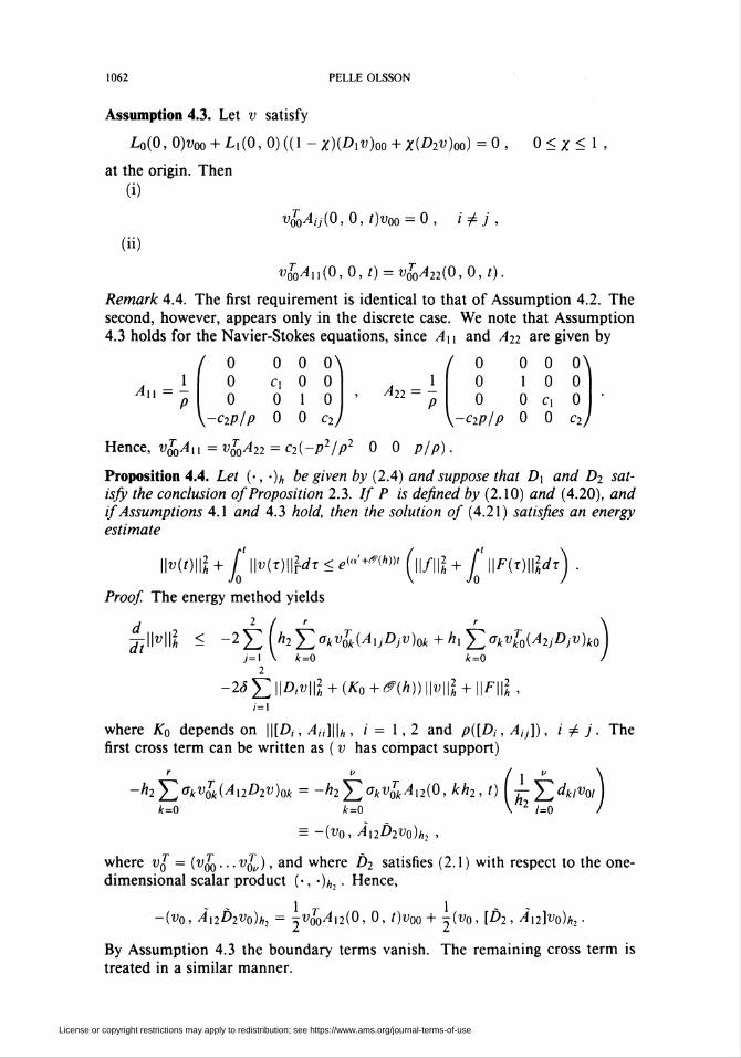
1062 PELLE OLSSON

Assumption 4.3. Let v satisfy

L0(0,0)voo + Lx(0,0)((l-x)(Dxv)oo + x(D2v)oo) = 0, 0<x< 1 ,

at the origin. Then

(i)

(ü)

v&AijiO, 0, t)vao = 0 , i¿j,

v&Axx(0,0,t) = v&A22(0,0,t).

Remark 4.4. The first requirement is identical to that of Assumption 4,2. The

second, however, appears only in the discrete case. We note that Assumption

4.3 holds for the Navier-Stokes equations, since Axx and A22 are given by

/

A 1^22 = T

0 0 0 0\0 c, 0 00 0 10

\-c2p/p 0 0 c2J

Hence, v$QAxx = v^A22 = c2(-p2/p2 0 0 p/p).

0 0 0 0\0 10 00 0 cx 0

\-c2p/p 0 0 c2)

Proposition 4.4. Let (•, •)„ be given by (2.4) and suppose that Dx and D2 sat-

isfy the conclusion of Proposition 2.3. // P is defined by (2.10) and (4.20), andif Assumptions 4.1 and 4.3 hold, then the solution of (4.21) satisfies an energyestimate

\\v(t)\\l + f \\v(x)\\2rdx < e(»'^(*))' (\\f\\2 + j*

Proof. The energy method yields

\mw\dx

n^ < ~2 Ï2 ( hl Y. akvlk(A\jDjV)ok + h\Y akVk(i(A2jDjV)k07=1 *=0 k=0

-là Y iiAuii2 + (Ko+em mil + \\n\l.i=\

where K0 depends on \\[D¡, Ait]\\h, i = 1, 2 and p([D¡, A¡j]), i ^ j . Thefirst cross term can be written as ( v has compact support)

r u / j i/ \

-h2YakVçJk(AnD2v)ok = -h2Yakv£kA\2(0, kh2, t) yYdk>vwk=0 k=0 1=0

= -(vq, Àx2D2v0)h2 ,

where v~ = (v7^...Vqv), and where D2 satisfies (2.1 ) with respect to the one-

dimensional scalar product )„,. Hence,

- . 1 T 1-(v0,Ai2D2v0)h2 = -v^Ai2(0,0, t)voo + -(v0, [D2, An]v0)h2

By Assumption 4.3 the boundary terms vanish. The remaining cross term is

treated in a similar manner.



Next, we take care of the boundary terms corresponding to the pure second

differences. Only the origin needs to be analyzed, since the other boundary

points are treated exactly as in the proof of Proposition 3.2. At the origin we

get (Au = Aii(0,0,t)) '

- h2o0VoQAxx(Dxv)oo - hxo0vl0A22(D2v)00

= -(hx+h2)o0v^((l-x)Axx(Dxv)oo + xA22(D2v)m) , x = h 'h ,

and, by Assumption 4.3,

- h2o0vl0Axx(Dxv)0o - hxo0v£0A22(D2v)oo

= -(h\ +h2)o()vl)Axx((l-x)(Dxv)m + x(D2v)c)o) .

But v = Pv implies Loxv = 0, i.e., by (4.19),

L0(0, 0)v00 + LX(0, 0) ((1 - x)(Dxv)oo + x(D2v)00) = 0.

In particular, LIlvm = 0. Partition vtj = v'^ + v'-j, where v7 G ker(L{),

v"j G ker(L{)-L. Assumption 3.1 then gives

- h2o0VooAxx(Dxv)oo - hxo0VmA22(D2v)oo

= -(/z, +h2)o0v¿0Axx {(l-x)(Dxv")oo + x(D2v")00) .

By construction,

L0(0, 0)^0 + ^,(0, 0) ((1 -x)(Dxv")00 + X(D2v")oo) =0 ,

which can be solved in exactly the same way as the corresponding equation in

the proof of Proposition 3.2. Hence,

- h2or,v£0Axx(Dxv)qo - hxo0v£0A22(D2v)oo

= h2o0vc]0AxxLxxLoVo0 + hxoovl0A22L~lL0Voo ,

where we again have invoked Assumption 4.3. We thus arrive at

i r

¡/¿IN* + INr ^ (2\AxxLxiL0\2,oo + p([D2,Äx2\) + l) h2 Yok\v0k\2k=0

r

+ (2\A22L7lL0\XrOO + p([Dx, Ä2X]) + l) hxY°k\vko\2k=0

-2ôY\\DiV\\2h + (K0+cf(h))\\v\\2 + \\F\\2,;'=1

where \v\Xt00 = sup(|nfc0|) and |v|2,oo = sup(|%t|). Replacing p([D¡,Aji])by |^,,|;,oo , i í } , one obtains the coefficients of the boundary terms of the

analytic energy estimate. They are thus identical if the coefficient matrices are

constant or if we use the standard second-order method. Finally, the bound-

ary terms of the right hand are eliminated by applying the one-dimensional

Sobolev inequality 2.6 in the xx- and x2-directions, respectively. This proves

the proposition, o


1064 PELLE OLSSON

Remark 4.5. It is clear from the proof that (4.21) is strictly stable if the coef-

ficient matrices are constant, or if Af¡ = A¡¡, í = 1,2, and the second-order

method (2.3) is used.

5. Summary and conclusions

We have demonstrated that for a given finite-dimensional scalar product

(•, -)h any linear discretized boundary condition can be written as an orthogonal

projection operator P that satisfies (u, Pv)h = (Pu, v)n . It should be noted

that the projection is well defined if the corresponding analytic problem is well

posed. For general boundary conditions one may also have to require that the

discretization parameter h be small enough (consistency). The projections P ,

the summation-by-parts property, and Proposition 2.4 constitute the main tools

needed to obtain an energy estimate for the semidiscrete case. For a large class

of problems it has been established that existence of an energy estimate for the

continuous problem implies the same for the semidiscrete system.

In one space dimension we are no longer required to consider restricted full

norms

fl \SO

£= i

v ■••/which were used in [4] to prove stability for symmetric hyperbolic systems sub-

ject to homogeneous boundary conditions. The main result is the stability proof

for mixed hyperbolic-parabolic systems subject to general linear boundary con-

ditions. Reformulating the analytic problem makes it possible to obtain strictstability, i.e., we have a time stable semidiscrete approximation that is bounded

by the same exponential growth rate (modulo cf(h)) as the analytic problem.

For the parabolic part the excess growth rate is induced by the discrete Sobolev

inequality. Furthermore, for the hyperbolic part we have used Assumption

2.1. In particular, strict stability is obtained for diagonal norms and variable-

coefficient problems, and for general norms and constant-coefficient problems.

The stability results hold for finite difference approximations of arbitrary order.

In two space dimensions we are forced to consider diagonal norms in order to

have summation by parts in both dimensions. Stability of high-order schemes

is obtained for general hyperbolic and parabolic initial-boundary value prob-

lems. All results obtained for two dimensions generalize to higher dimensions.

Furthermore, the stability results are valid even if there are corners present.

Although there are no general existence proofs for hyperbolic-parabolic prob-

lems on nonsmooth domains, it may still be useful to have stability results that

allow for corners since they appear in most multi-dimensional finite difference

implementations.The methods presented in this paper are similar to finite element methods

in that stability for the semidiscrete system follows more or less directly from

the corresponding continuous one. There is, however, one major difference:

The FEM technique often results in implicit space discretization, whereas the

discretized space operators reported in this paper always are explicit.



There are other ways of imposing boundary conditions so as to ensure time

stability (strict stability) when using difference operators satisfying a summation-

by-parts property. An elegant technique is proposed in [2]. A so-called Simulta-

neous Approximation Term, SAT for short, is added to the semidiscrete scheme.

The SAT will act as a penalty function to enforce an approximation of the dis-

crete boundary conditions. In [2] this approach is used to prove time stability

for high-order finite difference approximations of one-dimensional constant-

coefficient hyperbolic systems. Also, it is not necessary to consider identical

difference stencils in the interior. A new and interesting class of such difference

operators can be found in [1].

Acknowledgment

The author wishes to thank Professor Joseph Öliger for many stimulating

discussions on the topics of this paper.

Bibliography

1. M. Carpenter and J. Otto, High-order cyclo-difference techniques: A new methodology for finite

differences, Tech. report, ICASE, NASA Langley Research Center, Hampton, VA 23681-0001,1993.

2. D. Gottlieb, M. Carpenter, and S. Abarbanel, Time-stable boundary conditions for finite-

difference schemes solving hyperbolic systems: Methodology and application to high-order

compact schemes, Tech. Report 93-21, ICASE, NASA Langley Research Center, Hampton,

VA 23681-0001, 1993.

3. H.-O. Kreiss and J. Lorenz, Initial-boundary value problems and the Navier-Stokes equations,

Pure and Appl. Math., vol. 136, Academic Press, San Diego, CA, 1989.

4. H.-O. Kreiss and G. Scherer, Finite element and finite difference methods for hyperbolic

partial differential equations, Mathematical Aspects of Finite Elements in Partial Differential

Equations (C. de Boor, ed.), Academic Press, New York, 1974, pp. 195-212.

5. _, On the existence of energy estimates for difference approximations for hyperbolic

systems, Tech. Report, Dept. of Scientific Computing, Uppsala University, 1977.

6. P. Olsson, Stable approximation of symmetric hyperbolic and parabolic equations in several

space dimensions, Tech. Report 138, Dept. of Scientific Computing, Uppsala Univ., Uppsala,Sweden, December 1991.

7. _, Summation by parts, projections, and stability. II, Math. Comp., to appear.

8. G. Scherer, Numerical computations with energy estimates schemes, Tech. report, Dept. of

Scientific Computing, Uppsala Univ., Uppsala, Sweden, April 1977. In PhD thesis by G.

Scherer, 1977.

9. B. Strand, Summation by parts for finite difference approximations for d/dx, J. Comput. Phys.

110(1994), 47-67.

RIACS, Mail Stop T20G-5, NASA Ames Research Center, Moffett Field, California

94035-1000E-mail address: pelleariacs.edu


mathematics of computationvolume 64, number 211july 1995. pages s23-s26

Supplement to

SUMMATION BY PARTS, PROJECTIONS, AND STABILITY. I

PELLE OLSSON

Let F = /-E-,¿(¿TS-1L)-1¿T where L =( ¿„ ... ¿lr L0x L2i ... L2r ) rep-

resents homogeneous Neumann conditions (localized to the origin), cf. section on the

heat equation. For convenience we have v = 0.5 and h\ - h2 = 1. We shall show

that LJ0P = 0, which will follow if we can prove that ¿[„S"1 ¿(¿TE"' L)~xl7 = l7w.

Straightforward computations show that

where

¿rs-'z.

/ 1

IT,

Dm Du onDj2 D22 D23

D\3 D23 D33

D.i = D, , DU = D

*r )

( 1 \

and

Dx: r2DV2D23, DM = lfjL + &), * = ±dlk 2(T0

The inverse is given by

2 V^o

7.1 '12 '13

I TJ2 T22 T23

.3 '23 '33

<Tk

vitl.

Tu = r33 = ü-' +

Tn = Tl

1 — pa

/( — <tt4

D-,Di2Dl2Du7

(1 -/«r)(l-

7^22

13 (l-/«7)(l -<„->) "

(/t -JT4)(1 ^OTl)

(I -/«t)(1 -ar!) '

(T = Dj2Du'Du.

ß = trT* + -(\-<rTi)

^)0.|ö|2.

DU'DUD23D33\

© 1995 American Mathematical Society

S23


S24 SUPPLEMENT

kW! 4i

>WI

h- =

e •-

s 6,

S3 S -o

. . +o o c^

111I I

I

o o o o

o o o o

o » o o

O Tf "# O- I

o o o o

O O C! o

-12

lit7 O M)w -a "

II '0.

5.-=0 II

cew

ii ;s;s MZ s -

hw

~ -> o ^'

[2 S

v. as

Ce t/a

II

II

II+

ii

+

+

+

+

+

SIW

o -s Q


SUPPLEMENT S25

i iOv;

T■À

S-

W

W

II

w

I •■«:° I 5_

VI

+

VI

ià +

Il II

% 7

H II

h

o+

3 ^ N ii

5 ' I•W»

II

5

I

o+

G

II

s. "* »

v„S

.J c

il "E

«S E = y= — =

VI

«8VI

t. S


S26 SUPPLEMENT

nei

3 ^

> II

It

M

c

— ^

a ce

fes 05t 5 feii i U C

3 ^

id. Si

3 ""= '— ;r-

3 'C

Il I

S h

+

C5

aV

II


summation by parts, projections, and stability. i · summation by parts, projections, and...

Documents