Summer Number Theory Seminar 2001

Algebraic and Transcendental Numbers

Eric Patterson and Vladislav Shchogolev ∗

∗Research was supported by Columbia University VIGRE Fellowship and advised by grad-uate John Zuehlke.

1

Contents

1 Unique Factorization 3

2 Gaussian Integers 4

3 Groups, Rings, and Fields 5

4 Rational and Gaussian Primes 8

5 Congruences 8

6 Polynomials Over a Field 9

7 The Eisenstein Irreducibility Criterion 10

8 Symmetric Polynomials 10

9 Numbers Algebraic over a Field 12

10 Extensions of a Field 12

11 Algebraic and Transcendental Numbers 13

12 The Real Numbers are not Countable 14

13 The Sufficiency of Q 15

14 Decimal Expansions 16

15 Simple Irrationalities 16

16 Bases, Finite Extensions, Conjugates and Discriminants 20

17 Algebraic Integers and Integral Bases 22

18 Liouville Inequality and Transcendental Sums 24

19 The Generalized Lindemann Theorem 25

20 Units and Primes in Algebraic Number Fields 30

21 Cauchy’s Theorem 31

22 The Gelfond-Schneider Theorem 38

23 The Riemann Zeta-Function 40

24 Examples 40

2

Abstract

This paper reviews the topics covered in the 2001 Summer NumberTheory Seminar. All definitions and theorems will receive attention, butmost proofs will be excluded or abbreviated. Examples will be givenwhere the authors think necessary or interesting. This paper will focus onalgebraic and transcendental number theory, but many detours into otherareas of math will be made.

1 Unique Factorization

We begin by defining prime numbers.

Definition 1.1. The prime numbers are those numbers m which are differentfrom 0 and ±1 and which possess no factors other than ±1 and ±m.

With this definition, we can now state our goal for this section: establishthat every integer can be factored in one and only one way, apart from orderand sign, as the product of prime numbers (i.e., the Fundamental Theorem ofArithmetic). In the following discussion, we will assume that every collection,finite or infinite, of non-negative integers contains a smallest element.

Theorem 1.2. If a, b ∈ Z, b > 0, then ∃ integers q and r such that

a = bq + r 0 ≤ r < b.

The integers q and r are unique.

The proof follows from choosing q such that q ≤ a

band q + 1 >

a

b. The

result is shown to be unique by assuming two different solutions, which leadsto a contradiction of our choice of r. For instance, if a = 12 and b = 5, then wewould choose q = 2, which gives r = 2.

12 = 5 · 2 + 2

Definition 1.3. Two integers a and b are relatively prime if they share nofactors except ±1. We express this as (a, b) = 1.

For example, (12, 5) = 1.

Theorem 1.4. If (a, b) = 1, then ∃ s, t ∈ Z for which as + bt = 1.

Continuing with the same values of a and b, we can satisfy the above theoremwith s = −2 and t = 5:

12 · −2 + 5 · 5 = 1.

We get the same result for s = 7 and t = 17, so the theorem clearly does notclaim a unique result. The proof follows from a creative use of the divisibilitytheorem and the assumption about the existence of a smallest integer in a setof non-negative integers.

3

Definition 1.5. An integer m divides an integer n, written m | n, if there existsan integer q such that n = qm. Equivalently, m is a factor of n. Otherwise, mdoes not divide and is not a factor of n, written m - n.

Theorem 1.6. If p is a prime number and p | ab, then p | a or p | b.Proof. We choose to include the proof because it shows an interesting use ofTheorem 1.4. If p | a, we are done, so consider instead that p - a ⇒ (p, a) = 1.Thus, we can apply the previous theorem using integers l and m.

lp + ma = 1lbp + mab = b

p | ab ⇒ ab = pq

lbp + mpq = b

p(lb + mq) = b

p | b.

For instance, if a = 12 and b = 5, ab = 60. The primes 2, 3, 5 | 60, and eachone also divides a or b. A repeated application of this theorem gives a usefulcorollary.

Corollary 1.7. If a prime number p divides a product a1a2 · · · an of integers,then it divides at least one ai.

We will provide a formal definition of units in Section 20. For now, by aunit we mean an element that divides 1; for the rational integers, the units are±1. Finally, we arrive at our goal:

Theorem 1.8 (Fundamental Theorem of Arithmetic). Each integer notzero or a unit can be factored into the product of primes which are uniquelydetermined to within order and multiplication by units.

We will provide a brief sketch of the proof because this theorem is rathersignificant. If our integer is prime, we are done. If it is not prime, we must beable to factor it into two integers, not units. If these factors are primes, we aredone. Otherwise, continue the process. This process must terminate because afinite integer cannot be the product of an arbitrarily large number of integersall greater than one. If there are two such factorizations, we can conclude thateach factor must appear in each factorization to within multiplication by unitsbecause the factors are prime.

2 Gaussian Integers

We now define a new class of integers and ask the same questions we have askedabout integers. Consider the class G of Gaussian integers defined as:

G = {α = a + bi | a, b ∈ Z}.

4

For this class of numbers, we say that α divides β if there is a number γ ∈ Gsuch that β = αγ. An element of G is a unit if it divides 1, and therefore everyelement of G. A number π in G is prime if it is not zero or a unit and if everyfactorization π = αβ means that α or β is a unit.

With this terminology we can ask, do Gaussian integers have a unique fac-torization? To answer this question, we must first define the norm:

Definition 2.1. The norm N(α) of a Gaussian integer α = a+ bi is defined as:

Nα = αα = |α|2 = a2 + b2

We identify five important properties of the norm:

1. If α is in Z as well as in G, then Nα = α2

2. N(αβ) = Nα Nβ

3. Nα = 1 if and only if α is a unit.

4.

Nα =

0 if α = 0,1 if α = ±1 or ±i,> 1 otherwise.

5. If Nα is prime in Z, then α is prime in G.

Theorem 2.2. If α and β are Gaussian integers, β 6= 0, then ∃ integers π andρ such that

α = πβ + ρ, Nρ < Nβ

In proving this theorem we choose integers s and t such that

|A− s| ≤ 12, |B − t| ≤ 1

2where α/β = A + Bi

Then π = s + ti, ρ = α− πβ satisfies the theorem.

Theorem 2.3. If π is a prime and π|αβ, then π|α or π|β.

To prove this theorem we can proceed much as in the case of rational in-tegers. By the same analog, the Gaussian version of the fundamental theoremof arithmetic follows from this theorem. In other words, Gaussian integers dohave a unique factorization, within order and units.

3 Groups, Rings, and Fields

Before we address the topic of algebraic numbers, it will be useful to define theterms group, ring, and field.

5

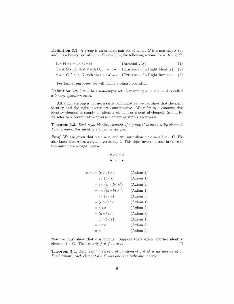
Definition 3.1. A group is an ordered pair 〈G, ◦〉 where G is a non-empty setand ◦ is a binary operation on G satisfying the following axioms for a, b, c ∈ G:

(a ◦ b) ◦ c = a ◦ (b ◦ c) (Associativity) (1)∃ e ∈ G such that ∀ a ∈ G, a ◦ e = a (Existence of a Right Identity) (2)∀ a ∈ G ∃ a′ ∈ G such that a ◦ a′ = e (Existence of a Right Inverse) (3)

For formal purposes, we will define a binary operation.

Definition 3.2. Let A be a non-empty set. A mapping ρ : A×A → A is calleda binary operation on A.

Although a group is not necessarily commutative, we can show that the rightidentity and the right inverse are commutative. We refer to a commutativeidentity element as simply an identity element or a neutral element. Similarly,we refer to a commutative inverse element as simply an inverse.

Theorem 3.3. Each right identity element of a group G is an identity element.Furthermore, this identity element is unique.

Proof. We are given that a ◦ e = a, and we must show e ◦ a = a ∀ a ∈ G. Wealso know that a has a right inverse, say b. This right inverse is also in G, so ittoo must have a right inverse.

a ◦ b = e

b ◦ c = e

e ◦ a = (e ◦ a) ◦ e (Axiom 2)= e ◦ (a ◦ e) (Axiom 1)

= e ◦ (a ◦ (b ◦ c)

)(Axiom 3)

= e ◦ ((a ◦ b) ◦ c

)(Axiom 1)

= e ◦ (e ◦ c) (Axiom 3)= (e ◦ e) ◦ c (Axiom 1)= e ◦ c (Axiom 2)= (a ◦ b) ◦ c (Axiom 3)= a ◦ (b ◦ c) (Axiom 1)= a ◦ e (Axiom 3)= a (Axiom 2)

Now we must show that e is unique. Suppose there exists another identityelement f ∈ G. Then clearly f = f ◦ e = e.

Theorem 3.4. Each right inverse b of an element a ∈ G is an inverse of a.Furthermore, each element a ∈ G has one and only one inverse.

6

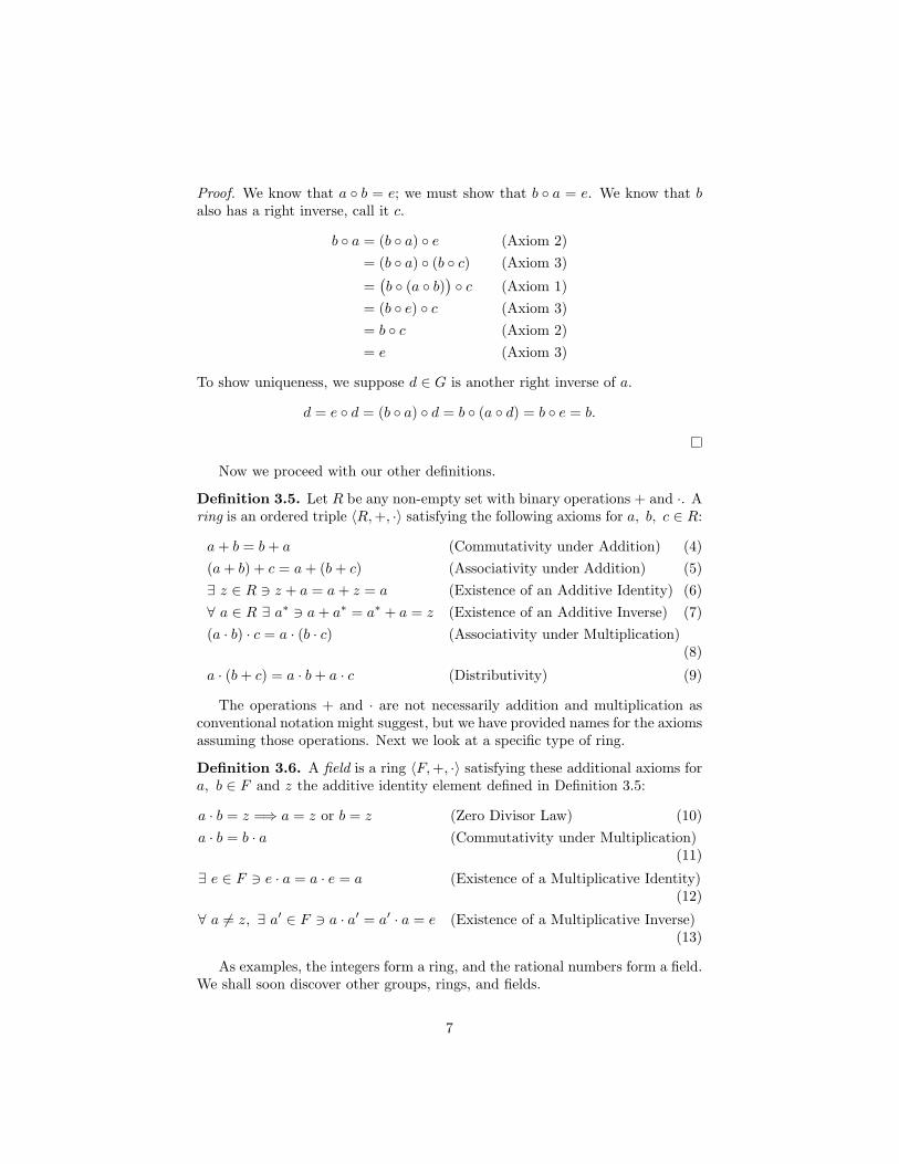
Proof. We know that a ◦ b = e; we must show that b ◦ a = e. We know that balso has a right inverse, call it c.

b ◦ a = (b ◦ a) ◦ e (Axiom 2)= (b ◦ a) ◦ (b ◦ c) (Axiom 3)

=(b ◦ (a ◦ b)

) ◦ c (Axiom 1)= (b ◦ e) ◦ c (Axiom 3)= b ◦ c (Axiom 2)= e (Axiom 3)

To show uniqueness, we suppose d ∈ G is another right inverse of a.

d = e ◦ d = (b ◦ a) ◦ d = b ◦ (a ◦ d) = b ◦ e = b.

Now we proceed with our other definitions.

Definition 3.5. Let R be any non-empty set with binary operations + and ·. Aring is an ordered triple 〈R, +, ·〉 satisfying the following axioms for a, b, c ∈ R:

a + b = b + a (Commutativity under Addition) (4)(a + b) + c = a + (b + c) (Associativity under Addition) (5)∃ z ∈ R 3 z + a = a + z = a (Existence of an Additive Identity) (6)∀ a ∈ R ∃ a∗ 3 a + a∗ = a∗ + a = z (Existence of an Additive Inverse) (7)(a · b) · c = a · (b · c) (Associativity under Multiplication)

(8)

a · (b + c) = a · b + a · c (Distributivity) (9)

The operations + and · are not necessarily addition and multiplication asconventional notation might suggest, but we have provided names for the axiomsassuming those operations. Next we look at a specific type of ring.

Definition 3.6. A field is a ring 〈F, +, ·〉 satisfying these additional axioms fora, b ∈ F and z the additive identity element defined in Definition 3.5:

a · b = z =⇒ a = z or b = z (Zero Divisor Law) (10)a · b = b · a (Commutativity under Multiplication)

(11)

∃ e ∈ F 3 e · a = a · e = a (Existence of a Multiplicative Identity)(12)

∀ a 6= z, ∃ a′ ∈ F 3 a · a′ = a′ · a = e (Existence of a Multiplicative Inverse)(13)

As examples, the integers form a ring, and the rational numbers form a field.We shall soon discover other groups, rings, and fields.

7

4 Rational and Gaussian Primes

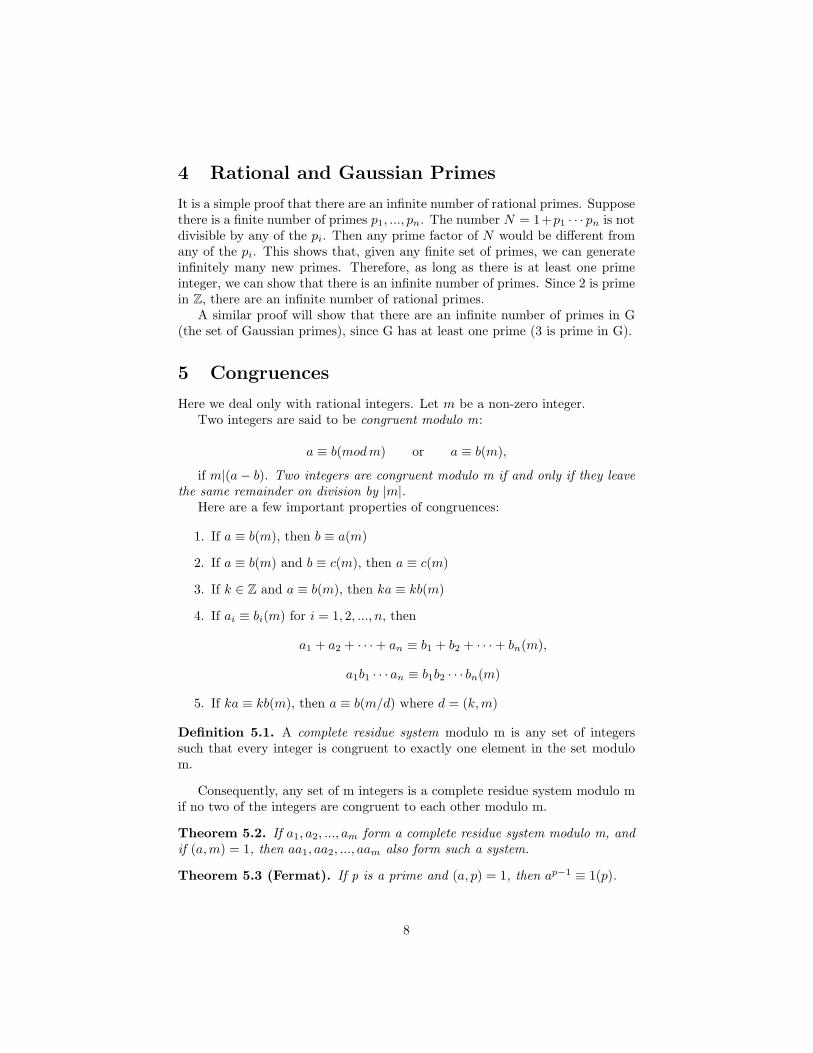
It is a simple proof that there are an infinite number of rational primes. Supposethere is a finite number of primes p1, ..., pn. The number N = 1+p1 · · · pn is notdivisible by any of the pi. Then any prime factor of N would be different fromany of the pi. This shows that, given any finite set of primes, we can generateinfinitely many new primes. Therefore, as long as there is at least one primeinteger, we can show that there is an infinite number of primes. Since 2 is primein Z, there are an infinite number of rational primes.

A similar proof will show that there are an infinite number of primes in G(the set of Gaussian primes), since G has at least one prime (3 is prime in G).

5 Congruences

Here we deal only with rational integers. Let m be a non-zero integer.Two integers are said to be congruent modulo m:

a ≡ b(modm) or a ≡ b(m),

if m|(a− b). Two integers are congruent modulo m if and only if they leavethe same remainder on division by |m|.

Here are a few important properties of congruences:

1. If a ≡ b(m), then b ≡ a(m)

2. If a ≡ b(m) and b ≡ c(m), then a ≡ c(m)

3. If k ∈ Z and a ≡ b(m), then ka ≡ kb(m)

4. If ai ≡ bi(m) for i = 1, 2, ..., n, then

a1 + a2 + · · ·+ an ≡ b1 + b2 + · · ·+ bn(m),

a1b1 · · · an ≡ b1b2 · · · bn(m)

5. If ka ≡ kb(m), then a ≡ b(m/d) where d = (k, m)

Definition 5.1. A complete residue system modulo m is any set of integerssuch that every integer is congruent to exactly one element in the set modulom.

Consequently, any set of m integers is a complete residue system modulo mif no two of the integers are congruent to each other modulo m.

Theorem 5.2. If a1, a2, ..., am form a complete residue system modulo m, andif (a,m) = 1, then aa1, aa2, ..., aam also form such a system.

Theorem 5.3 (Fermat). If p is a prime and (a, p) = 1, then ap−1 ≡ 1(p).

8

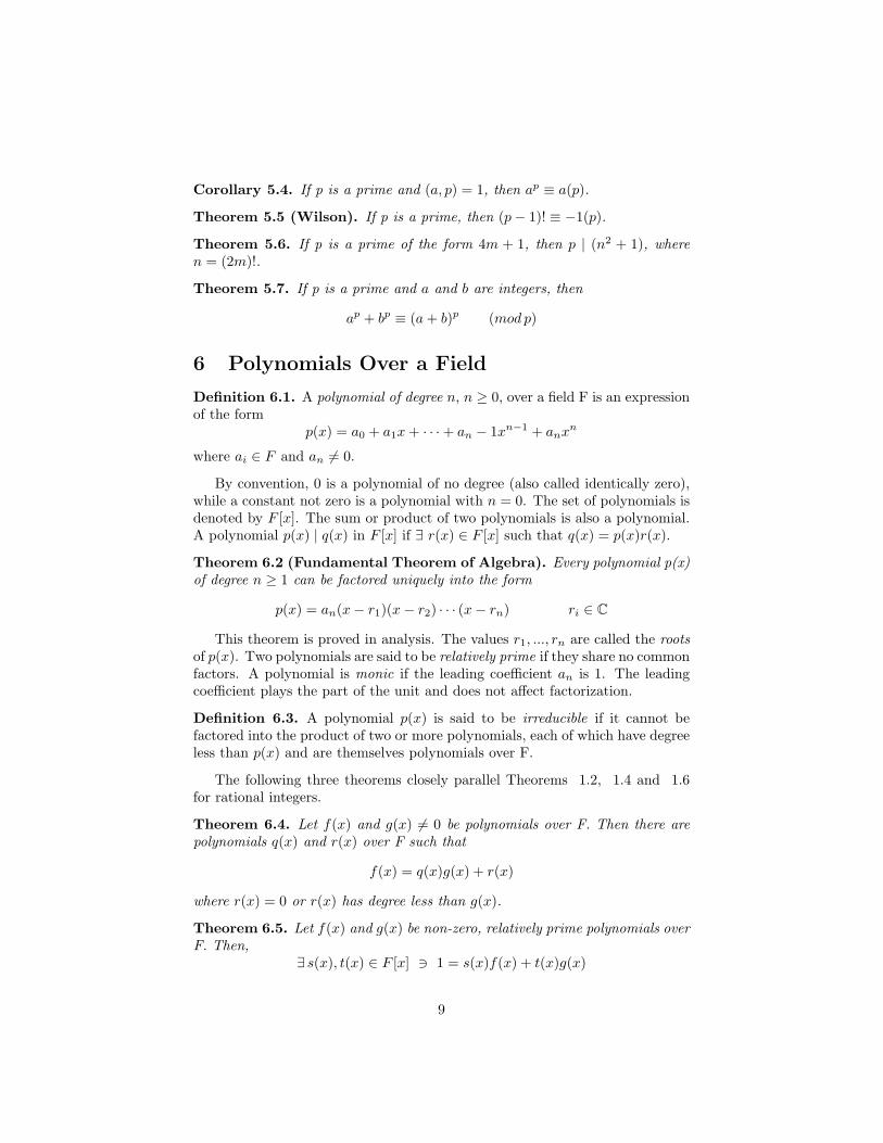
Corollary 5.4. If p is a prime and (a, p) = 1, then ap ≡ a(p).

Theorem 5.5 (Wilson). If p is a prime, then (p− 1)! ≡ −1(p).

Theorem 5.6. If p is a prime of the form 4m + 1, then p | (n2 + 1), wheren = (2m)!.

Theorem 5.7. If p is a prime and a and b are integers, then

ap + bp ≡ (a + b)p (mod p)

6 Polynomials Over a Field

Definition 6.1. A polynomial of degree n, n ≥ 0, over a field F is an expressionof the form

p(x) = a0 + a1x + · · ·+ an − 1xn−1 + anxn

where ai ∈ F and an 6= 0.

By convention, 0 is a polynomial of no degree (also called identically zero),while a constant not zero is a polynomial with n = 0. The set of polynomials isdenoted by F [x]. The sum or product of two polynomials is also a polynomial.A polynomial p(x) | q(x) in F [x] if ∃ r(x) ∈ F [x] such that q(x) = p(x)r(x).

Theorem 6.2 (Fundamental Theorem of Algebra). Every polynomial p(x)of degree n ≥ 1 can be factored uniquely into the form

p(x) = an(x− r1)(x− r2) · · · (x− rn) ri ∈ CThis theorem is proved in analysis. The values r1, ..., rn are called the roots

of p(x). Two polynomials are said to be relatively prime if they share no commonfactors. A polynomial is monic if the leading coefficient an is 1. The leadingcoefficient plays the part of the unit and does not affect factorization.

Definition 6.3. A polynomial p(x) is said to be irreducible if it cannot befactored into the product of two or more polynomials, each of which have degreeless than p(x) and are themselves polynomials over F.

The following three theorems closely parallel Theorems 1.2, 1.4 and 1.6for rational integers.

Theorem 6.4. Let f(x) and g(x) 6= 0 be polynomials over F. Then there arepolynomials q(x) and r(x) over F such that

f(x) = q(x)g(x) + r(x)

where r(x) = 0 or r(x) has degree less than g(x).

Theorem 6.5. Let f(x) and g(x) be non-zero, relatively prime polynomials overF. Then,

∃ s(x), t(x) ∈ F [x] 3 1 = s(x)f(x) + t(x)g(x)

9

Note that this theorem is a special case of Hilbert’s Nullstellensatz, whichdeals with a sum of arbitrarily many product pairs.

Theorem 6.6. Let p(x), f(x), g(x) be polynomials over F, p(x) irreducible,p(x) | f(x)g(x) over F, then p(x) divides f(x) or g(x).

7 The Eisenstein Irreducibility Criterion

Definition 7.1. A polynomial p(x) ∈ Z[x] is primitive if the coefficients haveno common factors beside ±1.

Theorem 7.2 (Gauss’ Lemma). The product of primitive polynomials isprimitive.

Note that any polynomial f(x) 6= 0 can be uniquely written in the formcff∗(x) where f∗ is primitive and cf is a positive rational number.

Theorem 7.3. If a polynomial p(x) ∈ Z[x] can be factored over Q, it can befactored into polynomials in Z[x].

Theorem 7.4 (Eisenstein’s irreducibility criterion). Let p be a prime andf(x) =

∑ni=0 aix

i ∈ Z[x] such that

p - an, p2 - a0; p | ai, i = 0, 1, ..., n− 1

Then f(x) is irreducible over R.

Let p be a prime. A polynomial of the form

xp − 1x− 1

= xp−1 + xp−2 + · · ·+ 1

is called cyclotomic. Substituting x+1 for x, we can show that this polynomialis irreducible by the Eisenstein criterion. The same technique can be used toshow that

xp2 − 1xp − 1

= xp(p−1) + xp(p−2) + · · ·+ xp + 1

is irreducible.

8 Symmetric Polynomials

Consider the independent variables x1, x2, . . . , xn. A polynomial in x1, x2, . . . , xn

over the field F is a finite sum of the form

g(x1, x2, . . . , xn) =∑

i1,i2,...,in

ai1,i2,...,inxi11 xi2

2 . . . xinn

where ai1,i2,...,in ∈ F and the ij ’s are positive integers.

10

Definition 8.1. A polynomial is symmetric if it is unchanged by any permu-tation of the variables.

For example, the following polynomials are symmetric:

x21 + x2

2 + x1x2

x21x

22 + x2

1x23 + x2

2x23 + 6x1x2x3.

A very useful polynomial when dealing with symmetric polynomials is the fol-lowing function of one variable z:

f(z) = (z − x1)(z − x2) · · · (z − xn)

= zn − σ1zn−1 + σ2z

n−2 − · · · (−1)nσn

σ1 = x1 + x2 + · · ·+ xn

σ2 = x1x2 + x1x3 + · · ·+ x1xn + x2x3 + x2x4 + · · ·+ xn−1xn

...σn = x1x2 · · ·xn

The σi are called the elementary symmetric functions in x1, x2, . . . , xn.

Theorem 8.2. Every symmetric polynomial in x1, x2, . . . , xn over a field Fcan be written as a polynomial over F in the elementary symmetric functionsσ1, σ2, . . . , σn. The result holds for polynomials with integer coefficients as well.

The theorem holds for integer coefficients because the proof only uses prop-erties of rings. The proof begins by separating the polynomial into homogeneouspolynomials and then defining a method for ordering the terms of the polyno-mial. For the highest term of the polynomial, there is a specific term of theelementary symmetric polynomials which will cancel the highest term in theoriginal polynomial, leaving a ”lower” degree polynomial. The process repeatsitself, and we get the desired result.

Theorem 8.3. Let f(x) be a polynomial of degree n over F with roots r1, r2, . . . , rn.Let p(x1, x2, . . . , xn) be a symmetric polynomial over F . Then p(r1, r2, . . . , rn)is an element of F.

Factoring f(x) into monic, first degree polynomials reveals that the elemen-tary symmetric functions evaluated at r1, r2, . . . , rn must be in F . Thus, theconclusion follows from the application of Theorem 8.2.

Corollary 8.4. Let f(x) and g(x) be polynomials over a field F , and let α1, α2, . . . , αn

and β1, β2, . . . , βk be their respective roots. Then the products

h1(x) =k∏

j=1

n∏

i=1

(x− αi − βj)

h2(x) =k∏

j=1

n∏

i=1

(x− αiβj)

11

are polynomials in x with coefficients in F .

The corollary follows directly from the preceding theorems and the product∏kj=1 f(x−βj). This corollary will have significant effects in some later sections.

9 Numbers Algebraic over a Field

Definition 9.1. A number θ is said to be algebraic over a field F if it satisfiesa polynomial in F [x]. θ is not necessarily in F.

Definition 9.2. The minimal polynomial for θ is the monic polynomial of leastdegree that is still satisfied by θ. Consequently a minimal polynomial is alsoirreducible.

Here are some important facts about minimal polynomials:

1. If θ is algebraic over F, it has a unique minimal polynomial.

2. Any polynomial satisfied by θ over F contains the minimal polynomial ofθ as a factor.

3. If f(x) and g(x) are relatively prime over F they have no roots in common.

4. An irreducible polynomial of degree n over F has n distinct roots.

The concept of minimal polynomials together with Corollary 8.4 can be usedto prove the following theorem:

Theorem 9.3. The totality of numbers algebraic over a field F forms a field. Inother words, the sum, product, difference and quotient of two algebraic numbersis also algebraic.

10 Extensions of a Field

Definition 10.1. Any field K containing another field F, is called an extensionof F. If θ is algebraic over F, then K = F (θ) is defined as the smallest fieldcontaining F and θ. K is called a simple algebraic extension of F.

Note that K would have to consist of all possible fractions f(θ)/g(θ) wheref(θ), g(θ) ∈ F [θ]. Any other expression in θ can be simplified into such aquotient. However, the next theorem states a stronger result:

Theorem 10.2. Every element α of F (θ) can be written uniquely in the form

α = a0 + a1θ + · · ·+ an−1θn−1 = r(θ)

where ai ∈ F and n is the degree of θ over F.

Definition 10.3. A multiple algebraic extension is the smallest field containingF and α1, ..., αn, a set of n algebraic numbers over F.

12

Theorem 10.4. A multiple algebraic extension of F is a simple algebraic ex-tension.

Theorem 10.5. If θ is algebraic over F, so is every element α of F (θ). Alsodegα ≤ degθ.

This theorem can be proved using symmetric polynomials or using a resultfrom linear algebra to show that α satisfies a polynomial over F.

11 Algebraic and Transcendental Numbers

Finally, we can define what we mean by an algebraic number. We denote theset of algebraic numbers by Q.

Definition 11.1. A number is an algebraic number if it is algebraic over thefield Q.

Now that we have defined an algebraic number, we want to show that ourdefinition has meaning. That is to say, we want to show that not all numbersare algebraic. This other class of numbers we call transcendental. We will usea construction by Liouville to show that transcendental numbers exist, but firstwe need a lemma.

Lemma 11.2. Let θ be a real algebraic number of degree n > 1 over Q. ∃ M >

1, which depends on θ, 3∣∣∣∣θ −

p

q

∣∣∣∣ ≥M

qn, ∀ p

q∈ Q with q > 0.

The proof of the lemma defines a function f(x) as the primitive of lowestdegree satisfied by θ. Then, it defines M ′ as the maximum of |f ′(x)| on theinterval [θ − 1, θ + 1]. M is defined as min

(1, 1

M ′). The proof then splits into

two cases:∣∣∣∣θ −

p

q

∣∣∣∣ ≥ 1, which is pretty straight forward, and∣∣∣∣θ −

p

q

∣∣∣∣ < 1, which

looks at∣∣∣∣f(θ)− f

(p

q

)∣∣∣∣ to get the appropriate result. Now we are equipped to

show that transcendental numbers exist.

Theorem 11.3 (Liouville). ∃ ξ 6∈ Q.

Proof. We include this proof because this seminar hinges on the existence oftranscendental numbers. Let ξ =

∑∞m=1(−1)m2−m! and denote by

ξk =pk

qk=

pk

2k!

the sum of the first k terms of the series for ξ. Then,∣∣∣∣ξ −

pk

qk

∣∣∣∣ = 2−(k+1)! − 2−(k+2)! · · · < 2−(k+1)! < 2−k·k! = q−kk .

13

First we suppose ξ is algebraic of degree n > 1 over Q. By the preceding

inequalities, qnk

∣∣∣∣ξ −pk

qk

∣∣∣∣ ≤ qn−kk . Letting k →∞, we find that

limk→∞

qnk

∣∣∣∣ξ −pk

qk

∣∣∣∣ = 0.

But by Lemma 11.2, ∃ M > 0 3∣∣∣∣ξ −

pk

qk

∣∣∣∣ ≥M

qnk

.

So

qnk

∣∣∣∣ξ −pk

qk

∣∣∣∣ ≥ M > 0

for all k, contrary to the limit 0.Next we suppose ξ ∈ Q (i.e., ξ is an algebraic number of degree 1). Thus,

ξ =p

q. Choose an odd k 3 2k+1 > q. Define

η = 2k!ξq − 2k!q

k∑m=1

(−1)m2−m! = 2k!q

∞∑

m=k+1

(−1)m2−m!.

This construction clears all denominators, so η ∈ N. But by our choice of k,

η < 2k!q1

2(k+1)!=

q

2k+1< 1,

a contradiction. Thus, ξ is transcendental.

This transcendental number may seem a little contrived, but it proves whatwe want to prove. Later we will discover that there are many transcendentalnumbers that are not so contrived.

12 The Real Numbers are not Countable

Definition 12.1. The mapping f : A → B is 1-1 if f(x1) 6= f(x2) wheneverx1 6= x2, for x1, x2 ∈ A.

Definition 12.2. The mapping f : A → B maps A onto B if f(A) = B.

Definition 12.3. If ∃ a 1-1 mapping of A onto B, then A ∼ B, and

1. A ∼ A

2. If A ∼ B, then B ∼ A.

3. If A ∼ B and B ∼ C, then A ∼ C.

14

Definition 12.4. For n ∈ N, let Jn be the integers 1, 2, . . . , n; J is the set ofall positive integers. For any set A,

1. A is finite if A ∼ Jn for some n including ∅.2. A is countable if A ∼ J .

3. A is uncountable if A is neither finite nor countable.

We assume that all real numbers have a unique binary representation. Ourdesired result will follow as a corollary from this theorem.

Theorem 12.5. Let A be the set of all sequences whose elements are the digits0 and 1. A is uncountable.

Proof. Let E be a countable subset of A, and let E consist of the sequencess1, s2, s3, . . . . We construct another sequence s by the following process: if thenth digit of sn is 1, then the nth digit of s is 0, and vice versa. Thus, thesequence s differs from every sequence in E by at least one place. Therefore,s 6∈ E, yet s 6∈ A. Therefore, E is a proper subset of A. Because E was anarbitrary countable subset of A, we conclude that all countable subsets of A areproper subsets of A. If A were countable, then it would be a countable subsetof itself. We have just shown that this would imply that A is a proper subsetof itself, an obvious contradiction.

Corollary 12.6. The real numbers are not countable.

Using the binary sequence a1, a2, a3, . . . with ai = 0 or 1, we express aunique real number for each sequence:

a1 · (10−1) + a2 · (10−2) + a3 · (10−3) + · · ·Thus, we have defined a function taking the binary sequences to a set of realnumbers. By Theorem 12.5, this set of real numbers in uncountable, and thusthe real numbers are uncountable.

13 The Sufficiency of QWe have defined

Q = {α | p(α) = 0 for some p(x) ∈ Z[x]}.Why don’t we introduce an extension of the algebraic numbers

Q = {β | p(β) = 0 for some p(x) ∈ Q[x]}?We do not talk of such a set because it does not introduce any new elements.

Theorem 13.1. Q = QThe proof constructs h(x) ∈ Z[x] by taking a product of fi(x) ∈ Q[x] where

each fi(x) has a unique permutation of the conjugates of the coefficients off1(x). We reach our conclusion about h(x) using symmetry arguments on itscoefficients.

15

14 Decimal Expansions

Here we present a few theorems that can be used to analyze numbers by lookingat their decimal expansions.

Theorem 14.1. Let a1, a2, ... be a sequence of positive integers, all greater than1. Then, any real number α is uniquely expressible in the form

α = c0 +∞∑

i=1

ci

a1a2 · · · ai

with integers ci satisfying the inequalities 0 ≤ ci ≤ ai − 1 for all i ≥ 1, andci < ai − 1 for infinitely many i.

Now we can present the next theorem for irrationality based on decimalexpansions.

Theorem 14.2. Let ai be as in the previous theorem, and let ci satisfy theresult. Assume that infinitely many of the ci 6= 0, and that each prime numberdivides infinitely many of the ai. Then α (as described in the previous theorem)is irrational.

15 Simple Irrationalities

We now turn our attention to some theorems that prove certain types of expres-sions yield irrational numbers.

Theorem 15.1. If the real number x satisfies an equation

xn + c1xn−1 + · · ·+ cn = 0

with each ci ∈ Z, then x is either an integer or an irrational number.

Proof. Suppose x ∈ Q, then x =a

bwith a, b ∈ Z, b > 0, and (a, b) = 1. Then

xn = −c1xn−1 − c2x

n−2 − · · · − cn

an

bn=

−1bn−1

(c1an−1 + c2a

n−2b + · · ·+ cnbn−1)

an = −b(c1an−1 + c2a

n−2b + · · ·+ cnbn−1).

If b > 1, then any prime divisor p of b would divide an =⇒ p | a and p | b, acontradiction of (a, b) = 1 =⇒ b = 1. So if x ∈ Q, then x ∈ Z. Otherwise, xmust be irrational.

We can construct some familiar irrational numbers from this theorem. Forexample,

√2 and

√3 satisfy x2 − 2 = 0 and x2 − 3 = 0, respectively. By the

theorem, these numbers are irrational. As a simple corollary, we provide thefollowing:

16

Corollary 15.2. If m is a positive integer which is not the nth power of aninteger, then n

√m is irrational.

Now we want to show that trigonometric functions taken at rational valuesgive irrational values. The methodology of this proof is repeated throughoutthis section, so we will provide the proof for the first theorem. Before we get tothat, we must provide two lemmas.

Lemma 15.3. If

h(x) =xng(x)

n!

where g(x) ∈ Z[x], then h(j)(0) ∈ Z for j = 0, 1, 2, . . . . Moreover, with thepossible exception of j = n, (n + 1) | h(j)(0). The possible exception for j = nis unnecessary if g(0) = 0.

The proof follows by looking at the explicit expression of h(j)(0).

Lemma 15.4. If f(x) is a polynomial in (r−x)2, then f (j)(r) = 0 for any oddinteger j.

Again, the proof follows from explicitly writing f (j)(r) = 0.

Theorem 15.5. For any non-zero r ∈ Q, cos r 6∈ Q.

Proof. Since cos−r = cos r, we will prove for r =a

bwith a, b ∈ N and b > 0.

Let

f(x) =xp−1(a− bx)2p(2a− bx)p−1

(p− 1)!=

(r − x)2p{r2 − (r − x)2}p−1b3p−1

(p− 1)!

where p is an odd prime to be specified.For 0 < x < r,

0 < f(x) <r2p{r2}p−1b3p−1

(p− 1)!=

r4p−2b3p−1

(p− 1)!.

LetF (x) = f(x)− f (2)(x) + f (4)(x)− f (6)(x) + · · · − f (4p−2)(x).

Thus,

d

dx{F ′(x) sin x− F (x) cos x} = F (2)(x) sin x + F ′(x) cos x− [F ′(x) cos x− F (x) sin x]

= F (2)(x) sin x + F (x) sin x

= f(x) sin x.

Using the Fundamental Theorem of Calculus, we find that∫ r

0

f(x) sin x dx = F ′(r) sin r − F (r) cos r + F (0).

17

By Lemma 15.4, f(x) is a polynomial in (r−x)2 =⇒ F ′(r) = 0. By Lemma 15.3,f(x) has the form of h(x) with n = p − 1 =⇒ p | f (j)(0) unless j = p − 1.Examining the p− 1st derivative, we find that

f (p−1)(0) =(p− 1)!a2p(2a)p−1

(p− 1)!= a2p(2a)p−1.

Thus, choosing p > a =⇒ p - f (p−1)(0) and p | f (j)(0) for all other j. Therefore,F (0) ∈ Z 3 p - F (0). Let F (0) = q; (p, q) = 1.

Now look at F (r).

f(r − x) =x2p{r2 − x2}p−1b3p−1

(p− 1)!

=x2p{a2 − b2x2}p−1bp+1

(p− 1)!

So f(r − x) has the form of h(x) from the lemma with n = p − 1 and g(x) =xp+1{a2 − b2x2}p−1bp+1. Thus, every f (j)(r) ∈ Z is divisible by p becauseg(0) = 0. For some m ∈ Z, F (r) = pm. Returning to the integral, we have

∫ r

0

f(x) sin x dx = −pm cos r + q.

Assume cos r ∈ Q; then cos r =d

k.

∫ r

0

f(x) sin x dx = −pmd

k+ q =⇒ k

∫ r

0

f(x) sin x dx = −pmd + kq

If we add another requirement to p: p > k =⇒ p - kq.

=⇒p - (−pmd + kq)=⇒− pmd + kq 6= 0

But −pmd + kq ∈ Z.∣∣∣∣k

∫ r

0

f(x) sin x dx

∣∣∣∣ < krr4p−2b3p−1

(p− 1)!

= kr3b2 {r4b3}p−1

(p− 1)!

=c1c

p−12

(p− 1)!

where the constants c1 = kr3b2 and c2 = r4b3 are independent of p. Thus, asp →∞,

c1cp−12

(p− 1)!→ 0.

18

Therefore, we can choose p sufficiently large so that

−1 < k

∫ r

0

f(x) sin x dx < 1.

Butk

∫ r

0

f(x) sin x dx = −qmd + kq

is a non-zero integer. Thus, we have a contradiction.

Corollary 15.6. π is irrational.

Proof. If π ∈ Q, then cos π 6∈ Q, but cos π = −1.

Corollary 15.7. The trigonometric functions are irrational at non-zero ratio-nal values of the arguments.

Proof. If sin r ∈ Q for r ∈ Q, r 6= 0, then 1 − 2 sin2 r = cos 2r ∈ Q. But thisconclusion contradicts the theorem since 2r ∈ Q.

If tan r ∈ Q for r ∈ Q, r 6= 0, then

cos 2r =1− tan2 r

1 + tan2 r∈ Q.

Again, we find a contradiction of the theorem.For the same r, csc r, sec r, cot r 6∈ Q because they are reciprocals of irra-

tionals.

Corollary 15.8. Any non-zero value of an inverse trigonometric function isirrational for rational arguments.

Proof. We will prove for arccos r because the other proofs are similar. Forr ∈ Q, assume arccos r = ρ ∈ Q. Then r = cos ρ is rational, contrary to thetheorem.

Theorem 15.9. The hyperbolic functions are irrational for non-zero rationalvalues of the arguments.

The proof of this theorem is almost identical to the proof of Theorem 15.5.The function F (x) does not alternate sign in this proof, and the function towhich we apply the Fundamental Theorem of Calculus is slightly different. Oncethe theorem is proven for cosh r, sinh r and tanh r follow by the same logic asthe above corollaries. We also get the same result for the inverse hyperbolicfunctions.

Theorem 15.10. If r ∈ Q, r 6= 0, then er 6∈ Q. If r ∈ Q, r > 0 and r 6= 1,then log r 6∈ Q.

19

Proof. We could proceed in a similar fashion as the previous two theorems,but instead we will use what we know about the hyperbolic functions. Sincer = log er, it suffices to prove for er. If er ∈ Q, then e−r ∈ Q, and so

cosh r =er + e−r

2∈ Q,

a contradiction.

Theorem 15.11. ∀ r ∈ Q, r > 0, logq r 6∈ Q unless r = qn for some n ∈ Z.

The proof follows from letting r =a

b, a fraction in lowest terms. Then,

assuming logqr =c

d, also a fraction in lowest terms, we get a contradiction by

showing that (c, d) 6= 1.

Theorem 15.12. e satisfies no relation of the form

amem + am−1em−1 + · · ·+ a1e + a0 = 0

for ai ∈ Z not all zero (i.e., e is transcendental).

We include this theorem in a section on irrationality because the method ofproof is similar to others in this section. We will not go through all the steps ofthe proof, but in analogy to the other similar proofs, we have

f(x) =xp−1(x− 1)p(x− 2)p · · · (x−m)p

(p− 1)!

F (x) = f(x) + f ′(x) + f (2) + · · ·+ f (mp+p−1)(x).

We differentiate e−xF (x) and apply the Fundamental Theorem of Calculus. Therest of the proof proceeds as expected with a few small variations.

16 Bases, Finite Extensions, Conjugates and Dis-criminants

Definition 16.1. K is an extension of F. A set of numbers in K, α1, α2, ..., αr

is linearly dependent (over F) if it is possible to find numbers c1, c2, ..., cr ∈ F ,not all zero, such that

c1α1 + c2α2 + · · ·+ crαr = 0.

Otherwise the numbers αi are linearly independent.

Definition 16.2. A set of numbers β1, β2, ..., βs in K forms a basis for K overF if for each β ∈ K, ∃ d1, d2, ..., ds ∈ F , unique numbers, such that

β = d1β1 + d2β2 + · · ·+ dsβs

20

A basis is consequently linearly independent, for otherwise the numberswould not be unique. Note that by Theorem 10.2, 1, θ, ..., θn−1 is a basis forF (θ).

Theorem 16.3. All bases for K over F have the same number of elements.

The previous theorem suggests the following definition. K is a finite exten-sion of degree n over F. We write n = (K/F ). Any n linearly independentelements in K form a basis for K.

Theorem 16.4. If α1, α2, ..., αn is a basis for K over F and

βj =n∑

i=1

aijαi , j = 1, 2, ..., n

where aij are in F, then β1, β2, ..., βn is also a basis if and only if det aij 6= 0.

Theorem 16.5. An extension K of F is finite if and only if it is a simplealgebraic extension.

The previous theorem equates the concepts of a finite extension and a simplealgebraic extension.

Theorem 16.6. If K is finite over F, and E over K, then E is finite over F.Moreover

(E/F ) = (E/K) · (K/F )

Corollary 16.7. If K is a finite extension of degree n over F, then any elementα of K is algebraic over F. Additionally, the degree of α divides n.

Theorem 16.8. If α satisfies the equation

αnxn + αn−1xn−1 + · · ·+ α0 = 0

where the αi are algebraic over F, then α is algebraic over F.

Let K = F (θ), n = (K/F ) and α ∈ K. The degree of α over F is m. Wecan write α uniquely as

α =n−1∑

i=0

ciθi = r(θ)

where ci ∈ F .

Definition 16.9. Denote the conjugates for θ as θ1, ..., θn. We can now definethe conjugates of α for F (θ):

αi = r(θi), i = 1, ..., n

Theorem 16.10. The conjugates of α for F (θ) are the conjugates over F (θ)each repeated n/m times. Secondly, α is in F if and only if all conjugates forF (θ) are the same. Lastly, F (α) = F (θ) if and only if all its conjugates forF (θ) are distinct.

21

Definition 16.11. Let α1, α2, ..., αn be a basis. Let α(i)j , i = 1, ..., n, be the

conjugates of αj for K. The discriminant for the basis is then:

4[α1, ..., αn] =∣∣∣α(i)

j

∣∣∣2

Theorem 16.12. The discriminant of any basis for F (θ) is in F and is neverzero. If F, θ and its conjugates are all real, then the discriminant of any basisis positive.

17 Algebraic Integers and Integral Bases

This section seeks to define integers in algebraic number fields. These resultswill prove useful in the proof of the Gelfond-Schneider Theorem.

We would like our definition of algebraic integers to fulfill the followingaxioms based on the behavior of the rational integers and Gaussian integers:

1. They form a ring.

2. If α is an integer in Q(θ), and α ∈ Q, then α ∈ Z.

3. If α is an integer, the conjugates of α are also integers.

4. If γ ∈ Q(θ), then nγ is an algebraic integer for some non-zero n ∈ Z.

We find that the following definition fulfills the desired axioms:

Definition 17.1. An algebraic number is an algebraic integer if its minimalpolynomial is in Z[x].

By our definition of conjugates, Axiom 3 must be satisfied. Axiom 2 clearlyfollows because the minimal polynomial of a rational number is of degree one,and if the it fits the definition of algebraic integer, then the minimal polynomialgives:

x + a0 = 0 =⇒ x = −a0 ∈ Z.

Now we want to show that the algebraic integers form a ring.

Lemma 17.2. If α satisfies any monic f(x) ∈ Z[x], then α ∈ I.The proof follows by dividing f(x) by the minimal polynomial of α and

noticing that the minimal polynomial must be monic with integral coefficients.

Theorem 17.3 (Verification of Axiom 1). If Q(θ) is an algebraic numberfield, then the integers in it form a ring.

Proof. We will prove that the algebraic integers are closed under addition; theother properties are similarly verified. We provide this proof because it revealsan important use of Corollary 8.4. Let α1, α2, . . . , αn and β1, β2, . . . , βk be theconjugates over Q of the algebraic integers α = α1 and β = β1, respectively.

22

By the conclusions in the Section 8, we know that the elementary symmet-ric functions evaluated at β1, β2, . . . , βk are integers, and thus, any symmetricpolynomial in β1, β2, . . . , βk is an integer.

Let f(x) be the minimal polynomial for α. Define

h(x) =k∏

j=1

f(x− βj).

The function f(x) has integral coefficients, so the coefficients of h(x) are sym-metric polynomials in β1, β2, . . . , βk with integral coefficients. Therefore, h(x) ∈Z[x]. Since f(x) is monic, so is h(x). Because f(α1) = 0, we get

h(α + β) = h(α1 + β1)

= f(α1 + β1 − β1)k∏

j=2

f(α1 + β1 − βj)

= 0.

By Lemma 17.2, α+β ∈ I. Also, α+β is closed in Q(θ) because α, β ∈ Q(θ).

Corollary 17.4. The totality of algebraic integers forms a ring.

The proof is exactly as above except that we do not restrict α and β to thesame algebraic number field. Another conclusion that we can reach by similarmeans is found in the next theorem.

Theorem 17.5. If α satisfies

f(x) = xn + γn−1xn−1 + · · ·+ γ0 = 0

for γi ∈ I, then α ∈ I.The proof defines

h(x) =∏(

xn + γ(in−1)n−1 xn−1 + · · ·+ γ

(i0)0

)

over all conjugates γ(ij)j . The rest mirrors the above proof.

Next, we prove that the fourth and final axiom follows from our definitionof algebraic integers.

Theorem 17.6 (Verification of Axiom 4). If θ is an algebraic number,∃ r ∈ Z, r 6= 0, 3 rθ ∈ I.Proof. We know that θ satisfies some

anxn + an−1xn−1 + · · ·+ a0 = 0

for ai ∈ Z. Thus, anθ satisfies

xn + an−1xn−1 + an−2anxn−2 + an−3a

2nxn−3 + · · ·+ a0a

n−1n = 0,

a monic polynomial with integer coefficients.

23

Now we move on to define integral bases.

Definition 17.7. A set of algebraic integers α1, α2, . . . , αs is an integral basisof Q(θ) if every algebraic integer α in Q(θ) can be uniquely expressed as

α = b1α1 + b2α2 + · · ·+ bsαs

with bi ∈ Z.

Lemma 17.8. An integral basis is a basis.

The proof follows from the definition of integral basis and the fact that∀ β ∈ Q ∃ r ∈ N 3 rβ ∈ I. Note that if degQ(θ) = n, then s = n.

Lemma 17.9. If α1, α2, . . . , αn is a basis of Q(θ) over Q consisting only ofalgebraic integers, then 4[α1, α2, . . . , αn] ∈ Z.

The proof follows directly from the axioms established at the beginning ofthis section and Theorem 10.2.

Theorem 17.10. Every algebraic number field has at least one integral basis.

This proof considers all bases whose elements are algebraic integers. Bythe lemma, the discriminants are integers, so we can choose the basis withdiscriminant of minimum absolute value. If we suppose that such a basis is notan integral basis, we can construct another basis with integer elements whosediscriminant has a smaller absolute value, contrary to our choice of basis.

Theorem 17.11. All integral bases for a field Q(θ) have the same discriminant.

The proof takes two arbitrary integral bases, and expresses each in terms ofthe other. Taking the discriminants reveals that the discriminants must be thesame.

18 Liouville Inequality and Transcendental Sums

Definition 18.1. Let α be an algebraic number, and I is the set of algebraicnumbers. Then den(α) denotes the least positive integer d, such that dα ∈ I.Definition 18.2. Let |α| denote the maximum of the absolute values of α andits conjugates.

Theorem 18.3 (Liouville inequality). If α is a nonzero algebraic numberwith deg(α) = n, then

log |α| ≥ −2nmax{log|α|, log den(α)}This inequality can be used to prove the following two theorems:

Theorem 18.4. If α is an algebraic number with 0 < |α| < 1, then∑∞

k=1 αk!

is transcendental.

Theorem 18.5. Let d be an integer greater than 1. If α is an algebraic numberwith 0 < |α| < 1, then

∑∞k=0 αdk

is transcendental.

24

19 The Generalized Lindemann Theorem

In this section, we will outline the logic behind the Generalized LindemannTheorem, a very interesting result of transcendental number theory. Becausethe theorem requires many preliminary lemmas, we will state the theorem nowso that the goal is clear from the beginning.

Theorem 19.1 (The Generalized Lindemann Theorem). Given any dis-tinct algebraic numbers α1, α2, . . . , αm, the values eα1 , eα2 , . . . , eαm are linearlyindependent over the field of algebraic numbers. Equivalently, the equation

m∑

j=1

ajeαj = 0

is impossible for a1, a2, . . . , am ∈ Q, not all zero.

Now we must provide the preliminary information. The proof requires manyresults from symmetric polynomials and algebraic fields; we will not repeattheorems which we have already proven.

Theorem 19.2. Let β1, β2, . . . , βn be roots of

f(x) = bxn + c1xn−1 + · · ·+ cn = 0

in which b, ci ∈ Z. Let P (x1, x2, . . . , xn) be symmetric in x1, x2, . . . , xn withrational coefficients. Then, P (β1, β2, . . . , βn) ∈ Q. If P has integer coefficientsand is of degree t, then btP (β1, β2, . . . , βn) ∈ Z.

Most of this theorem has been proven in the symmetric polynomial section.The last statement follows from the fact that bβ1, bβ2, . . . , bβn are roots of

bn−1f(x

b) = xn + c1x

n−1 + bc2xn−2 + · · ·+ bn−1cn = 0.

Lemma 19.3. Consider the q polynomials P1, P2, . . . , Pq in y1, y2, . . . , ym

Pj = f1(xj)y1 + f2(xj)y2 + · · ·+ fm(xj)ym

for j = 1, 2, . . . , q with coefficients fi(xj), where all the fi(x) ∈ F [x] for somefield F . The product

q∏

j=1

Pj

with the terms in y being collected has coefficients which are symmetric inx1, x2, . . . , xq.

Any permutation of the product clearly leaves the sum of terms in yi’s un-changed.

Now we must provide a new definition:

25

Definition 19.4. Q(θ) is normal over Q if any polynomial irreducible over Qthat has one root in Q(θ) has all roots in Q(θ).

Theorem 19.5. Given any algebraic numbers α1, α2, . . . , αs, ∃ θ ∈ Q 3 Q(θ) ⊃Q(α1, α2, . . . , αs) and Q(θ) is normal. That is to say, a multiple algebraic ex-tension can always be contained in a normal, simple algebraic extension.

The proof has two parts. First, we know that ∃ γ 3 Q(γ) = Q(α1, α2, . . . , αs).The conjugates of γ create a multiple algebraic extension that can be set equalto a simple algebraic extension of θ. Second, we show that Q(θ) is normal. Insimple terms, this is done by writing any element ρ of Q(θ) as a polynomialin the conjugates of gamma. Then, we create a new polynomial in x whichhas rational coefficients because of its symmetry properties. Also, ρ satisfies itsminimal polynomial and the new construction, the minimal polynomial dividesthe construction, and all roots of the construction are in Q(θ).

Lemma 19.6. Let Q(θ) be a normal algebraic extension of degree n over Q withconjugates θ = θ(1), θ(2), . . . , θ(n). These conjugates regarded as polynomials inθ, are merely permuted by the substitution of θ(i) for θ. More generally, ifF (x) ∈ Q[x], then the set

F (θ(1)), F (θ(2)), . . . , F (θ(n))

is permuted by the substitution of θ(i) for θ.

The proof of the lemma is more subtle than its statement may suggest. Ifthe minimal polynomial for θ is

xn + b1xn−1 + bn = 0,

then we need to use the reduction rule

θn = −b1θn−1 − · · · − bn

on the conjugates of θ written as polynomials in θ. After some manipulation,we reach a point where substitution of the conjugates creates a permutation orθ satisfies a polynomial of degree n− 1. Since θ is of degree n, we can agree onthe former conclusion.

Lemma 19.7. Any element γ of Q(θ) and its conjugates over Q(θ) satisfy apolynomial equation of degree n with integral coefficients.

The elementary symmetric polynomials in the conjugates of γ are symmetricpolynomials in the conjugates of θ. The elementary symmetric polynomials canconstruct the minimal polynomial for γ with rational coefficients. Multiplyingby the least common denominator finishes the proof.

Lemma 19.8. Consider

f(x) =m∑

j=1

ajxαj g(x) =

t∑

j=1

bjxβj

26

with non-zero complex coefficients aj and bj and αj , βj ∈ Q. Assume all αj

are distinct and all βj are distinct. Taking the product f(x)g(x) and combiningterms with equal exponents guarantees at least one non-zero coefficient.

We find a simple, normal algebraic extension Q(θ) which contains all αj ’sand all βj ’s. Then we write the αj ’s and βj ’s as polynomials in θ. After defininga method for ordering our terms, we find that we are guaranteed that the firstterm of the product has a unique exponent that will not cancel.

Now we can outline the proof of the Generalized Lindemann Theorem. Firstwe outline the proof of a modified version of the theorem, in which we onlyprove linear independence over the rational numbers.

Theorem 19.9. Given any m distinct algebraic numbers α1, α2, . . . , αm, thevalues eα1 , eα2 , . . . , eαm are linearly independent over Q.

Assumem∑

j=1

aj exp (αj) = 0

for aj ∈ Q, not all zero. Throw out all terms with aj = 0 and multiply throughby a suitable integer to get aj ∈ Z. Use Theorem 19.5 to write all

αj =n−1∑

i=0

rijθi.

Then we have conjugates

α(k)j =

n−1∑

i=0

rij(θ(k))i

for the n conjugates of θ, which will be distinct. The product

n∏

k=1

m∑

j=1

aj exp (α(k)j ) =

r∑

j=0

cj exp (βj) = 0 (14)

with distinct βj by collecting terms. Note that aj ∈ Z =⇒ cj ∈ Z, and byLemma 19.8 the cj do not vanish. In Equation (14), substituting θ(i) permutesthe factors and makes βj → β

(i)j .

⇒ 0 =r∑

j=0

cj exp (β(1)j ) =

r∑

j=0

cj exp (β(2)j ) = · · · =

r∑

j=0

cj exp (β(n)j ) (15)

Multiply the respective sums by exp {−β(1)0 }, exp {−β

(2)0 }, . . . , exp {−β

(n)0 }. Let

γ(i)j = β

(i)j − β

(i)0

27

for j = 1, 2, . . . , r and all i. Note that all γ(i)j 6= 0 because the β

(i)j are necessarily

distinct for fixed i. Equation (15) implies

0 = c0 +r∑

j=1

cj exp (γ(1)j ) = c0 +

r∑

j=1

cj exp (γ(2)j ) = · · · = c0 +

r∑

j=1

cj exp (γ(n)j ).

By Lemma 19.7, γ(1)j , γ

(2)j , . . . , γ

(n)j are roots of a polynomial with integer coef-

ficients

gj(z) = bjzn + · · · = bj

n∏

i=1

{z − γ(i)j }

for all j.Next, the proof makes use of the method found in the simple irrationality

section. We will provide the appropriate f(z) and F (z), but the details of thissection are excluded because we only intend to outline the proof.

f(z) =(b1b2 · · · br)prnzp−1{∏r

j=1 gj(z)}p

(p− 1)!

F (z) = f(z) + f ′(z) + · · ·We apply the Fundamental Theorem of Calculus to

{F (z) exp (−z)}′ = −f(z) exp (−z).

The only deviations from the established method is multiplication of the integralby cj and exp (γ(i)

j ) and summing over all i and j. The limits of the integral are

0 and γ(i)j .

After carrying out the prescribed method, the modified theorem is proven.Now we need to expand the proof to algebraic coefficients. We begin by assuming

m∑

j=0

ajeαj = 0 (16)

for aj , αj ∈ Q. Then we take conjugates of aj over some field Q(θ) containingall aj . Then,

q∏

i=1

m∑

j=1

a(i)j exp (αj) = 0.

Lemma 19.3 =⇒ the product has coefficients symmetric in θ(1), θ(2), . . . , θ(q).Then, Theorem 19.2 =⇒ the product has rational coefficients. And Lemma 19.8=⇒ the product is not identically zero. Thus Equation (16) implies a contra-diction of Theorem 19.9.

The Generalized Lindemann Theorem provides us with a simple way of prov-ing the transcendence of some common expressions.

Theorem 19.10. The following numbers are transcendental:

28

1. e and π

2. eα, sin α, cos α, tan α, sinhα, cosh α, and tanh α for every non-zero α ∈ Q.

3. log α, arcsin α, and the other inverses of functions in the second list.

Proof. The proof of this theorem has many redundancies, so we only provide afew select proofs.e: Let αj = j ∈ N ⊂ Q. Then e does not satisfy

m∑

j=0

ajej = 0 aj ∈ Q.

eα: ∀ α ∈ Q, j ∈ N, αj ∈ Q

=⇒m∑

j=0

aj(eα)j =m∑

j=0

ajeαj 6= 0 aj ∈ Q.

π: Assume π ∈ Q. The algebraic numbers form a field =⇒ iπ ∈ Q =⇒ eiπ istranscendental. This is a contradiction because eiπ = −1.sin α: Assume sin α ∈ Q. Let sin α = a. Then

eiα − e−iα − 2iae0 = cos α + i sin α− cos α + i sin α− 2i sin α = 0

contrary to the linear independence of eiα, e−iα, and e0 over Q.sinhα: If sinh α ∈ Q, then

eα − e−α

2∈ Q,

a contradiction.log α: Assume a = log α ∈ Q for α ∈ Q. Then ea = α ∈ Q. But a ∈ Q =⇒ ea =α is transcendental, a contradiction.

Theorem 19.11. If α1, α2, . . . , αn are linearly independent over Q, then eα1 , eα2 , . . . , eαn

are algebraically independent over Q.

We must show that∑

j1,j2,...,jn

cj1,j2,...,jn(eα1)j1(eα2)j2 · · · (eαn)jn 6= 0

for non-zero cj1,j2,...,jn ∈ Q. We can rewrite this expression as∑

j1,j2,...,jn

cj1,j2,...,jn exp (α1j1 + α2j2 + · · ·+ αnjn) 6= 0.

As long as the ji’s are not all zero, we know that not all terms vanish. The sumcannot be identically zero by the Generalized Lindemann Theorem.

29

20 Units and Primes in Algebraic Number Fields

We now wish to extend our concepts of units, primes, and divisibility to algebraicintegers. Consider integers in a fixed algebraic number field K = Q(θ).

Definition 20.1. For α, β ∈ K, α divides β, written α | β, ifα

βis an integer of

Q(θ).

Definition 20.2. ε is a unit if ε | 1.

Theorem 20.3. The units form a group under multiplication.

Proof. If we have two units a and b, then ∃ d and e 3

a · d = 1 b · e = 1.

Associativity holds because units are algebraic integers. We can show that,therefore, the units are closed under multiplication:

(a · b) · (d · e) = (a · d) · (b · e) = 1 =⇒ a · b | 1.

The multiplicative identity axiom is fulfilled by the unit 1. The multiplicativeinverse axiom follows from that fact that for any unit a ∃ d 3 a · d = 1 =⇒ d isa unit.

Definition 20.4. α is a prime if α 6= 0, α is not a unit, and any factorizationα = γβ =⇒ γ or β is a unit.

Definition 20.5. If α ∈ I of K and n = (K/Q), then α has n conjugatesα1, α2, . . . , αn forK. The norm of α, N(α) or Nα. is α1α2 · · ·αn.

Lemma 20.6. Nα ∈ ZThe norm of α is simply the constant term of α’s minimal polynomial raised

to some power, which is obviously an integer.

Lemma 20.7. N(αβ) = Nα ·Nβ

The lemma follows from the explicit expression of both sides of the equation.

Lemma 20.8. α is a unit ⇐⇒ Nα = ±1.

The lemma follows directly from the definition of unit, the definition of thenorm, and the previous lemma.

Theorem 20.9. If N(α) is a rational prime, α is prime in K.

The theorem follows from factoring α and taking the norm of the factor-ization. The converse does not hold. For example, 3 is a prime in Q(i), butN(3) = 9 in Q(i).

30

Theorem 20.10. Every integer in K, not zero or a unit, can be factored intoa product of primes.

The proof is identical to the proof of the Fundamental Theorem of Arithmeticexcept that one must take the norm of the factorization to guarantee that itstops.

Corollary 20.11. There are infinite primes in an algebraic field.

The same argument that we used for rational integers works here.

21 Cauchy’s Theorem

We digress into complex variables because we require results from them to provethe Gelfond-Schneider Theorem.

Definition 21.1. A subset A of C is disconnected if ∃ open sets U and V in Cthat obey the following three conditions:

1. U and V are disjoint

2. A⋂

U 6= ∅ and A⋂

V 6= ∅

3. A ⊂ U⋃

V

A set A is connected if it is not disconnected.

Definition 21.2. A non-empty set D in the complex plane that is both openand connected is a domain in C.

Definition 21.3. A sequence 〈zn〉 in C has the complex number z0 as anaccumulation point if ∀ ε > 0, ∆(z0, ε) contains zn for infinitely many values ofn.

Definition 21.4. A subset A of the complex plane is compact if each sequencein A has an accumulation point that belongs to A.

Theorem 21.5. Any pair of distinct points z0 and z1 in a plane domain D canbe made the endpoints of a polygonal arc lying in D.

Lemma 21.6. Suppose that U is an open set in the complex plane and that Kis a compact subset of U . ∃ a radius r > 0 3 ∀ z ∈ K, ∆(z, r) is contained inU .

Theorem 21.7 (Cantor’s Theorem). Suppose that 〈Kn〉 is a sequence ofnon-empty compact sets in C satisfying K1 ⊃ K2 ⊃ K3 · · · . Then

⋂∞n=1 Kn is

not empty.

31

Definition 21.8. A function f is analytic in U if U is a non-empty open subsetof the complex plane, f is a complex-valued function whose domain-set containsU , and f is differentiable at every point in U .

Definition 21.9. A path γ in the complex plane is a continuous function of thetype γ : [a, b] → C, where [a, b] is a closed interval of real numbers. The rangeof γ is called its trajectory, denoted by |γ|. The initial and terminal points areγ(a) and γ(b), respectively. When these values coincide, γ is a closed path.

Definition 21.10. A path γ(t) = x(t) + iy(t) for a ≤ t ≤ b is smooth if itsderivative γ(t) with respect to the real parameter t, γ(t) = x(t) + iy(t), existsfor each t in [a, b] and if the function γ is continuous on the interval [a, b].

A path is piecewise smooth provided there is a partition P : a = t0 < t1 <· · · < tn = b of the interval [a, b] with the property that the restriction of γ toeach of the intervals [tk−1, tk], 1 ≤ k ≤ n, is a smooth path.

Lemma 21.11. Let D be a domain in the complex plane, and let z0 and z1 bepoints of D, not excluding the case z0 = z1. ∃ a piecewise smooth path in Dwith initial point z0 and terminal point z1.

Lemma 21.12. Suppose that f : A → C and g : A → C are continuousfunctions and that γ and β are piecewise smooth paths in A.

∫

γ

[f(z) + g(z)] dz =∫

γ

f(z) dz +∫

γ

g(z) dz; (i)∫

γ

cf(z) dz = c

∫

γ

f(z) dz for any complex constant c; (ii)∫

−γ

f(z) dz = −∫

γ

f(z) dz; (iii)

if γ + β is defined, then∫

γ+β

f(z) dz =∫

γ

f(z) dz +∫

β

f(z) dz; (iv)∣∣∣∣∫

γ

f(z) dz

∣∣∣∣ ≤∫

γ

|f(z)| |dz| . (v)

Theorem 21.13. Suppose that a function f is continuous in an open set U andthat F is a primitive for f in U . If γ : [a, b] → U is a piecewise smooth path,then ∫

γ

f(z) dz =[F (z)

]γ(b)

γ(a)

.

In particular, under the above hypotheses it is true that∫

γ

f(z) dz = 0

for every closed, piecewise smooth path γ in U .

32

Lemma 21.14. If a function f is analytic in an open set U , then∫

∂Rf(z) dz =

0 for every closed rectangle R in U .

Lemma 21.15. If a function f is continuous in an open set U and analytic inU ∼ {z0} for some points z0 ∈ U , then

∫

∂R

f(z) dz = 0

∀ closed rectangle R ∈ U .

Lemma 21.16. Let ∆ be an open disk on the complex plane, and let f be acontinuous function in ∆ with the property that

∫∂R

f(z) dz for every closedrectangle R in ∆ whose sides are parallel to coordinate axes. Then f has aprimitive in ∆. In particular,

∫γ

f(z) dz = 0 for every closed, piecewise smoothpath γ in this disk.

Theorem 21.17 (Cauchy’s Theorem – Local Form). Suppose that ∆ isan open disk in the complex plane and that f is a function which is analytic in∆ (or, more generally, is continuous in ∆ and analytic in ∆ ∼ {z0} for somepoint z0 ∈ ∆). Then

∫γ

F (z) dz = 0 for every closed, piecewise smooth pathγ ∈ ∆.

This theorem follows from Lemma 21.15 and Lemma 21.16.

Lemma 21.18. Let γ be a piecewise smooth path in the complex plane, let hbe a function that is continuous on |γ|, and let k be a positive integer. Thefunction H defined in the open set U = C ∼ |γ| by

H(z) =∫

γ

h(ζ) dζ

(ζ − z)k

is an analytic function whose derivative is given by

H ′(z) = k

∫

γ

h(ζ) dζ

(ζ − z)k+1.

Definition 21.19. The winding number n(γ, z) of γ about z is defined by theformula

n(γ, z) =1

2πi

∫

γ

dζ

ζ − z.

Theorem 21.20 (Cauchy’s Integral Formula – Local Form). For a func-tion f analytic in an open disk ∆ and a closed piecewise smooth path γ in ∆,we have

n(γ, z)f(z) =1

2πi

∫

γ

f(ζ) dζ

ζ − z

∀ z ∈ ∆ ∼ |γ|.

33

Proof. Fixing a point z ∈ ∆ ∼ |γ| and considering the function g : ∆ → Cdefined as

g(ζ) =

[f(ζ)− f(z)ζ − z

if ζ 6= z,

f ′(z) if ζ = z

we see that g is analytic in ∆ ∼ {z}. It is also at least continuous at z. Thus,we can apply Theorem 21.17.

0 =∫

γ

g(ζ) dζ

=∫

γ

[f(ζ)− f(z)ζ − z

dζ

=∫

γ

f(ζ) dζ

ζ − z− f(z)

∫

γ

dζ

ζ − z

=∫

γ

f(ζ) dζ

ζ − z− 2πin(γ, z)f(z),

which gives our result

n(γ, z)f(z) =1

2πi

∫

γ

f(ζ) dζ

ζ − z.

Definition 21.21. A cycle or a piecewise smooth cycle is a finite sequence ofclosed piecewise smooth paths in the complex plane.

Definition 21.22. A cycle σ in an open set U is homologous to zero in U ifn(σ, 0) = 0 for every z in C ∼ U . Two cycles σ0 = (γ1, γ2, . . . , γp) and σ1 =(β1, β2, . . . , βq) in U are homologous in U if the cycle σ = (γ1, γ2, . . . , γp, −β1,−β2, . . . ,−βq) is homologous to zero in U . Two non-closed piecewise smoothpaths λ0 and λ1 in U are homologous in U if λ0 and λ1 share both the sameinitial point and the same terminal point and if the closed path γ = λ0 − λ1 ishomologous to zero in U .

Theorem 21.23 (Cauchy’s Theorem). For a cycle σ in an open set U ,∫σ

f(z) dz = 0 for every analytic function f in U ⇐⇒ σ is homologous to zeroin U .

Proof. Assume∫

σf(z) dz = 0 for every analytic function f in U . If z ∈ C ∼ U ,

then f : U → C defined by f(ζ) = (ζ − z)−1 is clearly analytic. Therefore,

0 =∫

σ

f(ζ) dζ =∫

σ

dζ

ζ − z= 2πin(σ, z).

That is to say, n(σ, z) = 0 for every z ∈ C ∼ U , and thus σ is homologous tozero in U .

34

Assuming that σ is homologous to zero in U has a more complicated proof,which we will only outline. Consider the set V = {z ∈ C ∼ |σ| : n(σ, z) = 0}.The set K = C ∼ V is compact, lies in U , and contains |σ|. Use Lemma 21.6 todetermine a δ > 0 3 ∀ z ∈ K, ∆(z, δ) lies inside U . Then, we can create a par-tition of the complex plane of non-overlapping closed squares of side length δ/2.K must be closed, so it can intersect only a finite number of these squares. Thedisks ∆j of radius δ/2 concentric with the squares Q1, Q2, . . . , Qr intersectingK must be contained by U and must contain the squares with which they areconcentric.

Consider an analytic function f in U . Fix a point z in the interior of a squareQm. The local Cauchy integral formula on the disk ∆m gives

f(z) = n(∂Qm, z)f(z) =1

2πi

∫

∂Qm

f(ζ) dζ

ζ − z.

For j 6= m, n(∂Qj , z) = 0, so

0 = n(∂Qj , z)f(z) =1

2πi

∫

∂Qj

f(ζ) dζ

ζ − z.

For any z in the interior of any Qj ,

f(z) =1

2πi

r∑

j=1

∫

∂Qj

f(ζ) dζ

ζ − z.

If we look at the sides of the squares, we notice that integration along the side ofone square cancels the integration from another side. The only integrations thatdo not cancel come from sides that are not shared and, thus, do not intersectK. Call these sides λ1, λ2, . . . , λq:

f(z) =1

2πi

q∑

k=1

∫

∂λk

f(ζ) dζ

ζ − z. (17)

Use Lemma 21.18 to show that Equation 17 holds for all z of |σ|. Assume

35

σ = (γ1, γ2, . . . , γp). Then use Equation 17 to get

∫

σ

f(z) dz =∫

σ

{1

2πi

q∑

k=1

∫

λk

f(ζ) dζ

ζ − z

}dz

=1

2πi

p∑

l=1

q∑

k=1

∫

γl

{∫

λk

f(ζ) dζ

ζ − z

}dz

=1

2πi

q∑

k=1

p∑

l=1

∫

λk

{∫

γl

f(ζ) dz

ζ − z

}dζ

=q∑

k=1

∫

λk

f(ζ)

{p∑

l=1

12πi

∫

γl

dz

ζ − a

}dζ

= −q∑

k−1

∫

λk

f(ζ){

12πi

∫

σ

dz

z − ζ

}dζ

= −q∑

k=1

∫

λk

f(ζ)n(σ, ζ) dζ

= −1∑

k=1

∫

λk

f(ζ) · 0 dζ = 0.

Theorem 21.24 (Cauchy’s Integral Formula). Suppose that a function fis analytic in an open set U and that σ is a cycle in U which is homologous tozero in this set. Then

n(σ, z)f(z) =1

2πi

∫

σ

f(ζ) dζ

ζ − z

∀ z ∈ U ∼ |σ|.The proof mirrors the local proof almost exactly.

Corollary 21.25. For a function f analytic in an open set U and cycles σ1

and σ2 in U that are homologous in this set,∫

σ1

f(z) dz =∫

σ2

f(z) dz.

Corollary 21.26. For a function f analytic in an open set U with non-closedpiecewise smooth paths λ0 and λ1 ∈ U that are homologous in this set,

∫

λ0

f(z) dz =∫

λ1

f(z) dz.

Definition 21.27. A subset E of U is a discrete subset of U if E has no limitpoint that belongs to U .

36

Definition 21.28. A function f has an isolated singularity at a point z0 ofthe complex plane provided there exists an r > 0 with the property that f isanalytic in the punctured disk ∆∗(z0, r), yet not analytic in the full open disk∆(z0, r).

Definition 21.29. A function f is analytic modulo isolated singularities in anopen set U under the following conditions: there is a discrete subset E of U ,the singular set of f in U , with the feature that f is analytic in the open setU ∼ E, but has a singularity at each point of E.

Using the notation from Definition 21.28, take for granted that f can berepresented in ∆∗ as f(z) =

∑∞n=−∞ an(z − z0)n. Then, we have the following

definitions:

Definition 21.30. f has a removable singularity at z0 if an = 0 for everynegative index n.

Definition 21.31. S(z) =∑∞

n=1 a−n(z − z0)−n is the singular part of f at z0.

Definition 21.32. The coefficient a−1 in the singular function S is called theresidue of f at z0, notated Res(z0, f).

Theorem 21.33 (Residue Theorem). For a function f analytic modulo iso-lated singularities in an open set U , E the singular set of f in U , and a cycleσ ∈ U ∼ E homologous to zero in U ,∫

σ

f(z) dz = 2πi∑

z∈E

n(σ, z)Res(z, f).

Proof. We will only outline this proof. Using the properties of E and n(σ, z),show that n(σ, z) 6= 0 for only finitely many points z ∈ E. Let these finitelymany points be ζ1, ζ2, . . . , ζp. Let V = (U ∼ E)

⋃{ζ1, ζ2, . . . , ζp}. Concludethat n(σ, z) = 0 ∀ z ∈ C ∼ V (i.e., σ is homologous to 0 in V ).

Let Sk be the singular part of f at the point ζk. Sk is analytic in C ∼ {ζk};f−Sk has a removable singularity at ζk. The function g = f−S1−S2−· · ·−Sp

is analytic in V except for removable singularities at ζ1, ζ2, . . . , ζp. Remove thesesingularities to make g analytic in V . Use Cauchy’s Theorem to assert

0 =∫

σ

g(z) dz =∫

σ

f(z) dz −p∑

k=1

∫

σ

Sk(z) dz

=⇒∫

σ

f(z) dz =p∑

k=1

∫

σ

Sk(z) dz.

Let S(z) =∑∞

n=1 a−n(z − ζ0)−n for an arbitrary ζ0 ∈ E. S converges normallyin C ∼ {ζ0}, and converges uniformly on |σ|, which allows the computation

∫

σ

S(z) dz =∫

σ

( ∞∑n=1

a−n

(z − ζ0)n

)dz =

∞∑n=1

a−n

∫

σ

dz

(z − ζ0)n

= a−1

∫

σ

dz

z − ζ0= 2πin(σ, ζ0)Res(ζ0, f).

37

Thus, we can conclude∫

σ

f(z) dz = 2πi

p∑

k=1

n(σ, ζk)Res(ζk, f) = 2πi∑

z∈E

n(σ, z)Res(z, f).

22 The Gelfond-Schneider Theorem

The Gelfond-Schneider Theorem gives the solution to Hilbert’s seventh problem,which was published in the year 1900. The theorem was proved in 1934 byGelfond and independently in 1935 by Schneider.

The theorem can be stated in the following two equivalent ways:

Theorem 22.1. If α and β are algebraic numbers with α 6= 0, α 6= 1, and ifβ 6∈ Q, then any value of αβ is transcendental.

Theorem 22.2. If α and γ are non-zero algebraic numbers, and if α 6= 1, then(log γ)/(log α) is either rational or transcendental.

The second version of the theorem implies that, for example,

log10 r =log r

log 10

is transcendental if r is not a power of 10.The following lemmas are useful in proving the theorem.

Lemma 22.3 (Vandermonde determinant). Consider a determinant withnon-zero element ρa

j in the j-th row and the 1 + a-th column, with j = 1, 2, ..., tand a = 0, 1, ..., t− 1. Then the determinant vanishes if and only if ρj = ρk forsome distinct pair of subscripts j, k.

Lemma 22.4. Consider m equations in n unknowns:

ak1x1 + · · ·+ aknxn = 0, k = 1, 2, · · · ,m,

with aij ∈ Z, and with 0 < m < n. Let the positive integer A be defined such thatA ≥ |aij | ,∀i, j. Then there is a non-trivial solution x1, x2, · · · , xn in rationalintegers of our m equations such that

|xj | < 1 + (nA)m/(n−m), j = 1, 2, · · · , n

Lemma 22.5. Consider consider a field K of finite degree, a subset I of algebraicintegers in K and p equations in q unknowns:

αk1ξ1 + · · ·+ αknξn = 0, k = 1, 2, · · · , p,

with αij ∈ I, and with 0 < p < q. Let A ≥ 1 be an upper bound on the absolutevalues of the coefficients and their conjugates , A ≥ ||αij || ,∀i, j. Then there is

38

a positive constant c depending on the field K and not on p, q or the coefficients,such that the equations have a non-trivial solution ξ1, ξ2, · · · , ξq in integers ofK such that

||ξk|| < c + c(cqA)p/(q−p), k = 1, 2, · · · , p

One application of the Gelfond-Schneider theorem is the following theorem,the Gaussian version of Fermat’s last theorem.

Theorem 22.6. If a, b, c are strictly positive integers and n is a Gaussianinteger, then the an + bn = cn has a solution only when n = ±1 and ±2.

Proof. Let n = p + iq where p, q ∈ Z. Then we can write our equation and itsconjugate:

ap+iq + bp+iq = cp+iq

ap−iq + bp−iq = cp−iq

We multiply the two together:

a2p + b2p + (ab)p(a

b

)iq

+ (ab)p

(b

a

)iq

= c2p

Let z = ab . Substituting z and multiplying by ziq we get:

(ab)pz2iq + (a2p + b2p − c2p)ziq + (ab)p = 0

Now ziq satisfies a polynomial with integer coefficients. However, we knowziq must be transcendental by the Gelfond-Schneider theorem, unless of coursez = 1 or q = 0.

If q = 0, then we have Fermat’s Last Theorem, and we are done.Otherwise, z = 1 and so a = b. Then we can take the norms of both sides

of our original equation, and solve for c:

2ap+iq = cp+iq

2ap = cp

c = ap√

2

Since c must be an integer, p = ±1. Then, dividing both sides of the firstequation by ap+iq, we get:

2 =( c

a

)p+iq

so q must be zero, and we are done.

39

23 The Riemann Zeta-Function

The zeta-function can be used to show that certain infinite sums yield transcen-dental numbers.

Definition 23.1. The Riemann ζ-function is defined as a function of real num-bers greater than 1 by

ζ(s) ≡∞∑

n=1

1ns

Definition 23.2. The kth Bernoulli number Bk is defined as k! times the kthcoefficient in the Taylor series for t

et−1

Theorem 23.3.

ζ(2k) = (−1)kπ2k 22k−1

(2k − 1)!

(−B2k

2k

).

This gives rise to the following examples:

ζ(2) =π2

6, ζ(4) =

π4

90, ζ(6) =

π6

945Note that the formula implies ζ(2k) is transcendental for all k.

24 Examples

This section demonstrates various conclusions from concepts developed in theprevious sections.Example 1. 1 and i form an integral basis for Q(i). Furthermore, Q(i) and G,the set of Gaussian integers, are the same set.

We already know that 1 and i are a basis for Q(i), so every integer α ∈ Q(i)can be written α = a + bi for a, b ∈ Q. We must show that a, b ∈ Z. Theminimal polynomial for α is

(x− a− bi)(x− a + bi) = x2 − 2ax + a2 + b2 = 0.

Because α is an algebraic integer, 2a, (a2 + b2) ∈ Z. Suppose that a and b arenot integers. Then

2a ∈ Z =⇒ ∃ p 3 a =p

2in which p is odd.

b ∈ Q =⇒ b =x

y

with (x, y) = 1. Then, ∃ k ∈ Z 3p2

4+

x2

y2= k

p2y2 + 4x2 = 4y2k.

40

Therefore,4 | p2y2 =⇒ 4 | y2 =⇒ 2 | y

because p is odd. So we can express y = 2r for some integer r.

p2r2 + x2 = 4r2k =⇒ r2 | x2 =⇒ r | xBut (x, y) = (x, 2r) = 1 =⇒ r = 1 =⇒ y = 2 =⇒ x is odd. The equation

p2 + x2 = 4k

implies that 4k must be an even positive integer because both p2 and x2 arepositive odd integers.

4 | 4k =⇒ 4 | (p2 + x2) =⇒ p2 ≡ −x2 mod 4

For the square of any odd integer, we have

(2x + 1)2 mod 4 = (4x2 + 4x + 1) mod 4 = 1 =⇒ 4 - (p2 + x2).

We see that a rational a implies a contradiction, but is it possible for a ∈ Zwhile b ∈ Q? Then, we would have

a2 +x2

y2= k.

But k − a2 ∈ Z, so this case implies that b ∈ Z.To show that G ∼ Q(i), recall the definition of G:

G = {α = a + bi | a, b ∈ Z}.We have just shown that all elements of Q(i) can be written in the same formas the elements of G.Example 2. If 1 and i form an integral basis for Q(i), then can we conclude thatthe algebraic extension of an algebraic integer θ of degree 2 has the integralbasis 1 and θ? A counter example is simple to find. Consider the polynomialx2 − 162 = 0, which has solutions x = ±9

√2. If we adjoin one solution with

the rational numbers, Q(9√

2), we can check our proposition. Any element ofQ(9

√2) can be written as a + b · 9√2 with a, b ∈ Q by Theorem 10.2. Let

a = 1 and b = 1/3. The algebraic number 1 + (1/3) · 9√2 = 1 + 3√

2 ∈ Q(9√

2)is actually an algebraic integer, contrary to 1/3 6∈ Z, as seen by its minimalpolynomial:

(x− 1− 3√

2)(x− 1 + 3√

2) = x2 − 2x− 17.

Example 3. Is there a relationship among the field extensionsQ(θ(1)

), Q

(θ(2)

), . . . ,

Q(θ(n)

)of the conjugates of algebraic numbers θ(1), θ(2), . . . , θ(n)?

We begin by looking at at a simple quadratic field extension Q(√

6), whichhas a basis 1 and

√6. We know by Theorem 16.11 that 1 and −√6 is also a

basis for Q(√

6)

because(

1−√6

)=

(1 00 −1

)(1√6

)

41

and ∣∣∣∣1 00 −1

∣∣∣∣ = −1 6= 0.

The field extension Q(−√6) of the conjugate of√

6 also has the basis 1 and −√6,so the field extensions share all elements, that is to say Q(

√6) = Q(−√6).

We find that the same conclusion can be reached about the field extensionsof conjugates of any minimal polynomial of degree 2. For a minimal polyno-mial over the rational numbers, we multiply through by the greatest commondenominator to get a polynomial of the form

ax2 + bx + c = 0, a, b, c ∈ Z

which is known to have solutions

x =−b±√b2 − 4ac

2a.

We can find find a matrix relationship between the bases of the field extensions

Q

(−b +

√b2 − 4ac

2a

)and Q

(−b−√b2 − 4ac

2a

)which has a nonzero determi-

nant: (1

−b−√b2−4ac2a

)=

(1 0−ba −1

)(1

−b+√

b2−4ac2a

)

and ∣∣∣∣1 0−ba −1

∣∣∣∣ = −1 6= 0.

This connection among field extensions of conjugates does not continue withalgebraic numbers of degree 3. Consider for example

x3 − 2 = 0

(note that we do not consider x3−1 = 0 because it is not a minimal polynomial).First we want to find all the conjugates, so we factor out the real solution andthen use the quadratic formula:

(x− 3

√2)(

x2 + 3√

2x + 3√

4)

= 0

x = 3√

2,3√

2

(−1± i

√3

2

).

The extension Q(

3√

2)

contains no complex numbers, so it does not contain theother conjugates of 3

√2.

Consider one of the other extensions, Q(

3√

2[(−1 + i

√3)/2

]), which has a

basis

1,3√

2

(−1 + i

√3

2

), and 3

√4

(−1− i

√3

2

).

42

So every α ∈ Q (3√

2[(−1 + i

√3)/2

])can be written as

α = a1 + a23√

2

(−1 + i

√3

2

)+ a3

3√

4

(−1− i

√3

2

)

with ai ∈ Q. If a2 = a3 = 0, then α ∈ Q. If either a2 or a3 6= 0, then α ∈ C.Therefore, the real irrational conjugate 3

√2 6∈ Q (

3√

2[(−1 + i

√3)/2

]). We also

find that

α 6= 3√

2

(−1− i

√3

2

)

because such an α has no rational term (a1 = 0) and no terms with 3√

4 (a3 = 0).We cannot choose a rational a2 such that

a23√

2

(−1 + i

√3

2

)= 3√

2

(−1− i

√3

2

).

This conclusion holds generally for minimal polynomials of the form

x3 − n = 0

for n ∈ Q. Notice that such a polynomial is minimal as long as n 6= q3 for anyq ∈ Q. We might suppose an exception exists if n2 = p3 for some p ∈ Q becauseit will change the third basis element. This exception actually does not existbecause if n2 = p3, then ∃ q ∈ Q such that n = q3. This conclusion followsfrom applying the Fundamental Theorem of Arithmetic to the numerator anddenominator of n2 = p3 =

x

y. Factoring x into a product of primes reveals

that every prime must be raised to at least the sixth power for our equality tohold. Similarly, y is a product of primes to at least the sixth power. Thus, thenumerator and denominator of n are products of primes to at least the thirdpower.

Example 4. Let ω =−1 + i

√3

2and σ =

−1− i√

32

. We have found that

Q(

3√

2), Q

(3√

2ω), and Q

(3√

2σ)

are different fields. If we adjoin all three, weknow we can find an equivalent simple algebraic extension Q (θ).

We use the method used in the proof of Theorem 10.3 to find Q(θ) =Q

(3√

2, 3√

2ω). Let α1 = β3 = 3

√2, α2 = β1 = 3

√2ω, and α3 = β2 = 3

√2σ.

Then we must find the x’s that satisfy:

α1 + xβ1 = α1 + xβ2

α1 + xβ1 = α1 + xβ3

α1 + xβ1 = α2 + xβ2

α1 + xβ1 = α2 + xβ3

α1 + xβ1 = α3 + xβ2

α1 + xβ1 = α3 + xβ3.

43

These solutions are: x = 0,−σ, 1, ω. We can pick any other x, say x = 2, andlet

θ = α1 + xβ1 = 3√

2 + 2 · 3√

2ω = i3√

2√

3.

The fact that Q(i 3√

2√

3)

= Q(

3√

2, 3√

2ω)

follows from the rest of the proof.We could then try to find a γ such that Q(γ) = Q

(i 3√

2√

3, 3√

2σ), which would

require finding the minimal polynomial for i 3√

2√

3 and then finding all its con-jugates. Instead, we notice that

3√

2σ =−12

(i 3√

2√

3) +−136

(i 3√

2√

3)4,

so 3√

2σ ∈ Q(i 3√

2√

3). For any α ∈ Q(θ), Q(θ, α) = Q(θ) because Q(θ, α) isdefined to be the smallest field containingQ and both θ and α. Q(θ) fits this defi-nition. Therefore Q( 3

√2σ, i 3

√2√

3) = Q(i 3√

2√

3), and thus Q( 3√

2, 3√

2ω, 3√

2σ) =Q(i 3

√2√

3).

Example 5. The proof of Theorem 19.5 suggests a method for generating normalsimple algebraic extensions; namely, a simple algebraic extension equal to amultiple algebraic extension of conjugates will always be normal.

For some γ ∈ Q of degree n, we have conjugates γ1, γ2, . . . , γn. By Theo-rem 10.3, there exists θ such that Q(γ1, γ2, . . . , γn) = Q(θ). For any ρ ∈ Q(θ),we must show that all conjugates of ρ are also in Q(θ). By a generalization ofTheorem 10.2, any element of Q(θ) = Q(γ1, γ2, . . . , γn) can be written as a poly-nomial in of γ1, γ2, . . . , γn with rational coefficients (instead of a polynomial inθ with rational coefficient). Let ρ = f(γ1, γ2, . . . , γn). Let

G(x) =∏

{x− f(γi1 , γi2 , . . . , γin)}

over all permutations of i1, i2, . . . , in. The coefficients of G(x) are symmetricpolynomials in its roots f(γi1 , γi2 , . . . , γin). Any permutation of γ1, γ2, . . . , γn

merely permutes the f(γi1 , γi2 , . . . , γin) among themselves. Thus, the coeffi-cients of G(x) are symmetric polynomials in γ1, γ2, . . . , γn and so are rationalnumbers by Theorem 8.3. The polynomials g(x) and G(x) share the root ρ,and because g(x) is minimal, g(x) must be a factor of G(x). But all roots ofG(x) = 0 are elements of Q(θ) because they can all be written as polynomials inγ1, γ2, . . . , γn. All roots of g(x) = 0 are also roots of G(x) = 0 because g(x) isa factor of G(x); therefore, all roots of g(x) = 0 are elements of Q(θ) as desired.

In Example 4, we found thatQ(i 3√

2√

3) = Q( 3√

2, 3√

2ω, 3√

2σ) where 3√

2, 3√

2ω,and 3

√2σ are conjugates of x3 − 2 = 0. Therefore, Q(i 3

√2√

3) is normal.

Example 6. The set of all polynomials with integer coefficients is countable.We have already agreed that every set of positive integers has a smallest

element. Thus, a set of infinitely many unique positive integers will have aunique smallest element. We can map such a set to the positive integers byletting the smallest element correspond to 1. If we remove the smallest elementfrom the set, we will have a new unique smallest element, which will correspondto 2. We can continue this pattern to map a set of infinitely many uniquepositive integers to the positive integers.

44

If we can map the set of polynomials ∈ Z[x] to a set of positive integers, thenthat set can be mapped to the positive integers, from which we can concludeour desired result.

We assign two primes to each term of a polynomial in ascending order. Theconstant term will be assigned 2 and 3; the first degree term will be assigned 5and 7; the second degree term will be assigned 11 and 13; and so on. We haveproven that there exist infinitely many primes, so this method of assignmentcan account for a polynomial of any degree. The smaller prime assigned to eachterm will stand for a positive coefficient, and the larger prime will stand fora negative coefficient. The primes will be raised to the absolute value of theircoefficients; for a polynomial of degree n, notice that only n primes will be raisedto powers even though we will have 2n possible primes for that polynomial. Weassign a number to the polynomial by multiplying together all the primes totheir appropriate powers. For instance, the polynomial

12x3 − 7x2 + 8x− 2

would be assigned the number

32 · 58 · 137 · 1712 = 128526614147073132472630078125.

As we can see, the assigned numbers get incredibly large very easily. Neverthe-less, we know that each such number is unique from the Fundamental Theoremof Arithmetic. Thus, we have mapped the set of polynomials ∈ Z[x] to a setof infinitely many unique rational integers, which can be mapped to the set ofpositive integers. Thus, the set of polynomials ∈ Z[x] is countable.

Note that not all positive integers will be assigned a polynomial. For exam-ple, 12 = 22 · 3, which would imply that the constant term has both a positiveand a negative coefficient. Also, the ordering of the polynomials does not relateany information about their complexity (not in the imaginary sense). For in-stance, x2+x+1, which is assigned 2·5·11 = 110, would probably be consideredmore complex than x − 20, which is assigned 320 · 5 = 17433922005. We canuse a similar method for proving the countability of polynomials ∈ Q[x], butwe would need three primes per term (one for a positive numerator, one for anegative numerator, and one for the denominator) causing the assigned numbersto become even larger. If we agreed that polynomials with the same solutionswere equivalent and did not need separate numbers, we could map Q[x] → Z[x].Unfortunately, polynomials ∈ Z[x] could be equivalent with different numbers,such as x2+x+1 and 2x2+2x+2. Therefore, the attempt to assign one numberto polynomials with the same solutions is laborious because we would have todetermine which polynomials are equivalent in this way.

Similarly, the countability of the algebraic numbers is possible but labori-ous. First, we would only order minimal polynomials; thus, we would have tocheck each polynomial for this feature. Second, we would start the assignmentof primes to coefficients with 3 instead of 2. We would reserve 2 to indicatewhich solution to our polynomial we desired. We would order the solutions first

45

according to their arguments in the complex plane, and then by their magni-tudes. The number assigned to the first solution would have a factor of 2, thatassigned to the second would have a factor of 22, etc.

Example 7. We can use Lemma 22.5, which we used in the Gelfond-SchneiderTheorem, to find a bound for the solutions to a set of equations:

α11ξ1 + α12ξ2 + · · ·+ α1qξq = 0α21ξ1 + α22ξ2 + · · ·+ α2qξq = 0

...αp1ξ1 + αp2ξ2 + · · ·+ αpqξq = 0

in which 0 < p < q and αij ∈ Q. We will work out a specific example in whichαij ∈ Q(i). Let αij = i + j

√−1, p = 3, and q = 4:

(1 + i)ξ1 + (1 + 2i)ξ2 + (1 + 3i)ξ3 + (1 + 4i)ξ4 = 0(2 + i)ξ1 + (2 + 2i)ξ2 + (2 + 3i)ξ3 + (2 + 4i)ξ4 = 0(3 + i)ξ1 + (3 + 2i)ξ2 + (3 + 3i)ξ3 + (3 + 4i)ξ4 = 0.

Notice that maxi,j ‖αij‖ = ‖3 + 4i‖ = 25. Recall that ‖ξj‖ < c + c(cqA)p

q−p .We have determined A ≤ 25, so we have only to determine c in our bound.According to the proof, we choose c > hc2 and c > h maxj ‖βj‖ in whichh = degQ(i) = 2, 1 + c1 maxj ‖βj‖ > c2 ≥ c1 maxj ‖βj‖, c1 > max(i,j)

maxi,j‖αij‖ , andβj are the basis elements of Q(i). So we choose βj to be 1 and i; maxj ‖βj‖ = 1;425

< c1 = 1; c2 = 1 · 1 = 1; and thus 2 < c = 3. Therefore,

‖ξj‖ < 3 + 3(3 · 4 · 25)3 = 27000003.

We see that even for the simple algebraic numbers we constructed, this boundgets very large.

Example 8. We can rewrite some simple symmetric polynomials in the elemen-tary symmetric polynomials to demonstrate Theorem 8.2. We begin with

x21 + x2

2 + · · ·+ x2n.

Using the method in the proof, we know we will need the elementary symmetricpolynomials

σ21 =(x2

1 + x22 + · · ·+ x2

n)+ 2(x1x2 + x1x3 + · · ·+ x1xn + x2x3 + . . . xn−1xn)

σ2 =x1x2 + x1x3 + · · ·+ x1xn + x2x3 + . . . xn−1xn.

Then, we can writex2

1 + x22 + · · ·+ x2

n = σ21 − 2σ2.

46

We can similarly treat

x31 + x3

2 + · · ·+ x3n,

for which we will need

σ31 =(x3

1 + x32 + · · ·+ x3

n)

+ 3(x21x2 + x2

1x3 + · · ·+ x21xn + x2

2x3 + · · ·+ xn−1x2n)

+ 3(x1x2x3 + x1x2x4 + · · ·+ xn−2xn−1xn)

σ1σ2 =(x21x2 + x2

1x3 + · · ·+ x21xn + x2

2x3 + · · ·+ xn−1x2n)

+ 3(x1x2x3 + x1x2x4 + · · ·+ xn−2xn−1xn)

σ3 =(x1x2x3 + x1x2x4 + · · ·+ xn−2xn−1xn).

Then we see that

x31 + x3

2 + · · ·+ x3n = σ3

1 − 3σ1σ2 + 6σ3.

Example 9. Define roots of unity to be solutions to polynomials of the form

xk − 1 = 0

for positive integers k. For example, ±1 and−1± i

√3

2are roots of unity. We

can show that the roots of unity form a group under multiplication.First, we show that for roots of unity α and β, αβ is also a root of unity.

By definition, there exist positive integers l and m such that

αl − 1 = 0 βm − 1 = 0

αl = 1 βm = 0.

Therefore,(αl)m = 1m = 1 and (βm)l = 1l = 1.

Let k = l ·m so that αβ satisfies

xk − 1 = 0

because(αβ)lm = (αl)m · (βm)l = 1.

We have established that multiplication is a binary operator on this set.Associativity must hold because these are all algebraic numbers. The root ofunity 1 satisfies the criterion for the multiplicative identity. Now we show thata multiplicative inverse exists. Let α satisfy xl−1 = 0. The equation xl−1 = 0gives l roots of unity α = α1, α2, . . . , αl. We can factor our polynomial

(x− α1)(x− α2) · · · (x− αl) = 0

47

where each αi also satisfies xl − 1 = 0 (i.e., αli = 1). When we take the product

α1α2 · · ·αl we must get the constant term of the polynomial, 1. Let the inverseof α be

1α1

= α2α3 · · ·αl.

This number satisfies xl − 1 = 0 because(

1α1

)l

− 1 = (α2α3 · · ·αl)l − 1

= αl2α

l3 · · ·αl

l − 1

= 1l1l · · · 1l − 1= 1− 1= 0.

Example 10. In this example, we look at a few properties of polynomials of theform xn − 1 = 0.

Roots of such polynomials must all have a norm of 1 on the complex plane.Therefore they can be written in the form eiθ. These roots are always locatedon a unit circle, separated by equal angles of rotation.

To see this, label the roots xk, ordered by their arguments. Then xk = eiθk .Substituting into the polynomial

(eiθk)n − 1 = 0

eiθkn = ei2πk where k ∈ ZTherefore:

θkn = 2πk

θ

2π=

k

n

Since k is an integer, the θk must be distributed evenly. This also meansthat the k’s are a complete residue system modulo n.

Raising any root to an integer power is equivalent multiply its angle θ bythat power, thereby rotating to a different root on the circle. Therefore, raisingthe k-th root to successive integer powers will yield all the other roots if andonly if (k, n) = 1.

Example 11. Now we can prove a more general version of Theorem 15.1:

Theorem 24.1. Given a polynomial

f(x) = cnxn + · · ·+ c0 = 0

where cnc0 6= 0, then then for any rational roots ab , where (a, b) = 1, of f(x),

a | c0 and b | cn.

48

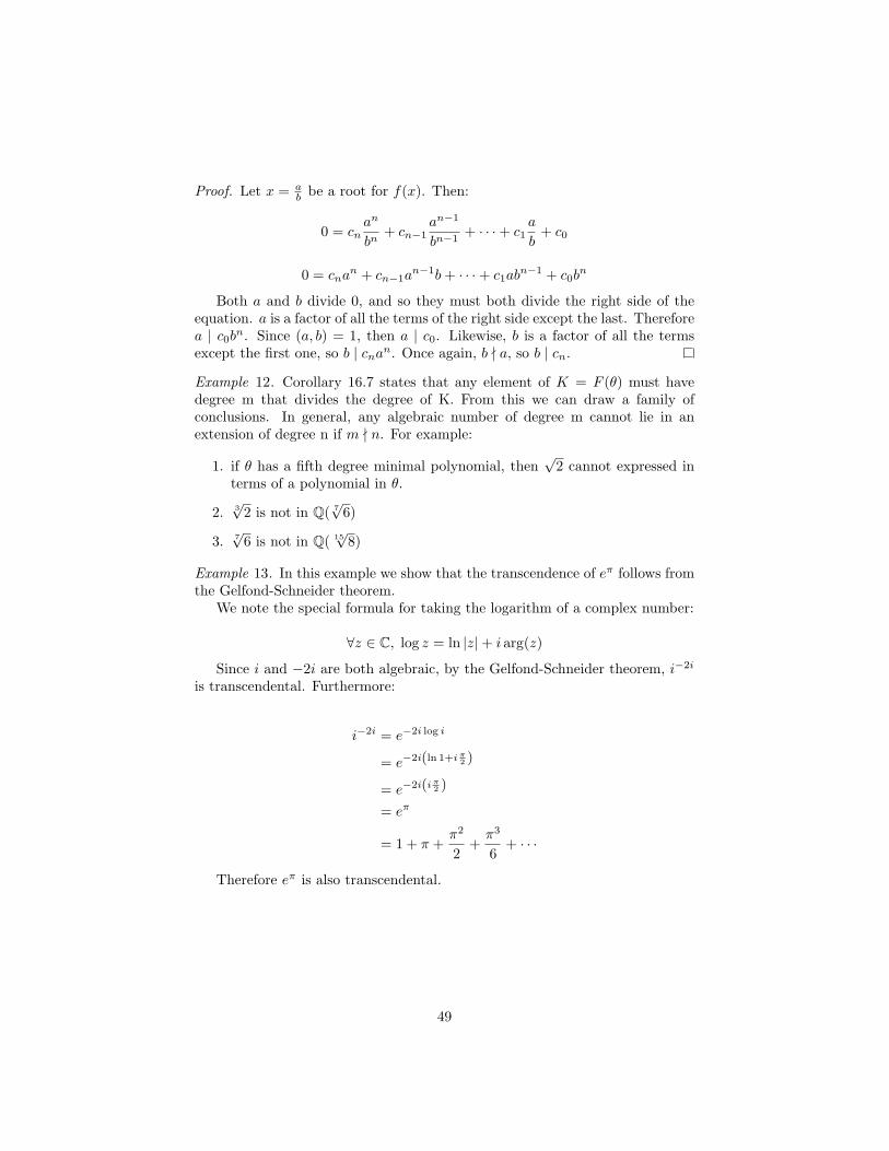
Proof. Let x = ab be a root for f(x). Then:

0 = cnan

bn+ cn−1

an−1

bn−1+ · · ·+ c1

a

b+ c0

0 = cnan + cn−1an−1b + · · ·+ c1abn−1 + c0b

n

Both a and b divide 0, and so they must both divide the right side of theequation. a is a factor of all the terms of the right side except the last. Thereforea | c0b

n. Since (a, b) = 1, then a | c0. Likewise, b is a factor of all the termsexcept the first one, so b | cnan. Once again, b - a, so b | cn.

Example 12. Corollary 16.7 states that any element of K = F (θ) must havedegree m that divides the degree of K. From this we can draw a family ofconclusions. In general, any algebraic number of degree m cannot lie in anextension of degree n if m - n. For example:

1. if θ has a fifth degree minimal polynomial, then√

2 cannot expressed interms of a polynomial in θ.

2. 3√

2 is not in Q( 7√

6)

3. 7√

6 is not in Q( 15√

8)

Example 13. In this example we show that the transcendence of eπ follows fromthe Gelfond-Schneider theorem.

We note the special formula for taking the logarithm of a complex number:

∀z ∈ C, log z = ln |z|+ i arg(z)

Since i and −2i are both algebraic, by the Gelfond-Schneider theorem, i−2i

is transcendental. Furthermore:

i−2i = e−2i log i

= e−2i(ln 1+i π2 )

= e−2i(i π2 )

= eπ

= 1 + π +π2

2+

π3

6+ · · ·

Therefore eπ is also transcendental.

49

References

[1] Robert E. Greene and Steven G. Krantz, Function Theory of One ComplexVariable, Wiley, New York, 1997.

[2] Neal Koblitz, p-adic Numbers, p-adic Analysis, and Zeta Functions, Gradu-ate Texts in Mathematics, Springer-Verlag, New York, 1977.

[3] Joseph Landin, Introduction to Algebraic Structures, Dover, New York, 1989.

[4] Kumiko Nishioka, Mahler Functions and Transcendence, Lecture Notes inMathematics 1631, Springer-Verlag, Berlin, 1996.

[5] Ivan Niven, Irrational Numbers, Fourth ed., Carus Mathematical Mono-graphs, Mathematical Association of America, 1997.

[6] Bruce P. Palka, An Introduction to Complex Function Theory, Undergradu-ate Texts in Mathematics, Springer-Verlag, New York, 1991.

[7] Harry Pollard and Harold G. Diamond, The Theory of Algebraic Numbers,Third ed., Dover, New York, 1998.

[8] Walter Rudin, Principles of Mathematical Analysis, Second ed., McGraw-Hill, New York, 1964.

[9] John Zuelke Fermat’s Last Theorem for Gaussian Integer Exponents, Amer-ican Mathematical Monthly, Vol. 106.1, Jan. 1999, p. 49.

50