sums of multiplicative functions andrew...
TRANSCRIPT
SUMS OF MULTIPLICATIVE FUNCTIONS
Andrew Granville
Abstract. In these six hours of lectures we will discuss three themes that have been centralto multiplicative number theory in the last few years: The uncertainty principle, bounds forcharacter sums, and mean values of multiplicative functions. I will discuss many recent devel-opments, in historical context, involving some proofs. The notes here are “pieced together”from several old articles of mine (mostly with Soundararajan, some alone, and some withFriedlander), so apologies to the reader for any disjointedness.
1. The Uncertainty Principle, in the twentieth century1.1. The distribution of Primes1.2. Maier matrices1.3. And beyond
2. The Uncertainty Principle, in the twenty-first century2.1. A general phenomenon2.2. The new framework2.3. Oscillations in mean-values of multiplicative functions2.4. More Examples
3. Halasz’s theorem3.1. The Halasz-Montgomery theorem3.2. Integral delay equations – a model for mean values3.3. An integral delay equation version of Proposition 3.13.4. An uncertainty principle for integral equations3.5. Spectra3.6. Sieving extrema
4. Character Sums4.1. The Polya-Vinogradov Theorem4.2. Burgess’s Theorem4.3. Improving Burgess’s Theorem? Integral delay equations
5. Pretentiousness5.1. Proof of the prime number theorem5.2. Interlude: Distance and beyond5.3. A new (and easy) application of pretentiousness5.4. Polya-Vinogradov revisited
6. Recent work6.1. Pretentiousness is indeed repulsive6.2. Multiplicative functions in arithmetic progressions6.3. Exponential sums6.4. The prime number theorem in terms of multiplicative functions6.5. Periodic functions pretending to be characters
Typeset by AMS-TEX
1

2 ANDREW GRANVILLE
1. The Uncertainty Principle, in the twentieth century1
1.1. The distribution of Primes. As a boy of 15 or 16, Gauss determined, by studyingtables of primes, that the primes occur with density 1
log x at around x. This translates intothe guess that
π(x) := #primes ≤ x ≈ Li(x) where Li(x) :=∫ x
2
dt
log t∼ x
log x.
The existing data lend support to Gauss’s guesstimate:
x π(x) = #primes ≤ x Overcount: [Li(x)− π(x)]
108 5761455 753109 50847534 17001010 455052511 31031011 4118054813 115871012 37607912018 382621013 346065536839 1089701014 3204941750802 3148891015 29844570422669 10526181016 279238341033925 32146311017 2623557157654233 79565881018 24739954287740860 219495541019 234057667276344607 998777741020 2220819602560918840 2227446431021 21127269486018731928 5973942531022 201467286689315906290 19323552071023 1925320391606803968923 7250186214
Notice how the entries in the final column are always positive and always about half thewidth of the entries in the middle column: So it seems that Gauss’s guess is alwaysan overcount by about
√x. We believe that this observation is both right and wrong:
Although the last column looks to be positive and growing we believe that it eventuallyturns negative, and changes sign infinitely often (see, e.g. [GM]). On the other handwe believe that the error in Gauss’s guess is never much more than
√x — correctly
formulated this statement is equivalent to the Riemann Hypothesis: In 1859, Riemann,in a now famous memoir, illustrated how the question of estimating π(x) could be turnedinto a question in analysis: Define ζ(s) :=
∑n≥1 n−s for Re(s) > 1, and then analytically
continue ζ(s) to the rest of the complex plane. We have, for sufficiently large x,
(1.1) xb−ε ¿ maxy≤x
|π(y)− Li(y)| ¿ xb+ε where b := supζ(β+iγ)=0
β.
The (as yet unproven) Riemann Hypothesis (RH) asserts that b = 1/2 (in fact that β = 1/2whenever ζ(β + iγ) = 0 with 0 ≤ β ≤ 1) leading to the sharp estimate
(1.2a) π(x) = Li(x) + O(x1/2 log x) .
1This section is an edited version of [Gr1].

OTTAWA NOTES 3
It was not until 1896 that Hadamard and De La Vallee Poussin independently provedthat β < 1 whenever ζ(β + iγ) = 0, which implies The Prime Number Theorem: that is,Gauss’s prediction that
π(x) ∼ Li(x) ∼ x
log x.
The best version known has an error term in which we do not even save a power of x:
π(x) = Li(x) + O
(x
/exp
(c(log x)3/5
(log log x)1/5
)).
In 1914, Littlewood showed, unconditionally, that
(1.2b) π(x)− Li(x) = Ω±
(x1/2 log log log x
log x
),
the first proven ‘irregularities’ in the distribution of primes2.Since Gauss’s vague ‘density assertion’ was so prescient, Cramer [Cra] decided, in
1936, to interpret Gauss’s statement more formally in terms of probability theory, to tryto make further predictions about the distribution of prime numbers: Let Z2, Z3, . . . be asequence of independent random variables with
Prob(Zn = 1) =1
log nand Prob(Zn = 0) = 1− 1
log n.
Let S be the space of sequences T = z2, z3, . . . and, for each x ≥ 2 define
πT (x) =∑
2≤n≤x
zn .
The sequence P = π2, π3, . . . , where πn = 1 if and only if n is prime, belongs to S. Cramerwrote: “In many cases it is possible to prove that, with probability 1, a certain relationR holds for sequences in S ... Of course we cannot in general conclude that R holds forthe particular sequence P , but results suggested in this way may sometimes afterwardsbe rigorously proved by other methods.” For example Cramer was able to show, withprobability 1, that
maxy≤x
|πT (y)− Li(y))| ∼√
2x · log log x
log x,
which corresponds well with the estimates in (1.2); and if true for T = P implies RH, by(1.1).
Gauss’s assertion was really about primes in short intervals, and so is best applied toπ(x+ y)−π(x), where y is “small” compared to x. The binomial random variables Zn aremore-or-less the same for all integers n in such an interval. If we take y = λ log x so that
2f(x) = Ω±(g(x)) means that there exists a constant c > 0 such that f(x+) > cg(x+) and f(x−) <−cg(x−) for certain arbitrarily large values of x±.

4 ANDREW GRANVILLE
the ‘expected’ number of primes, λ, in the interval is fixed then we would expect that thenumber of primes in such intervals should follow a Poisson distribution. Indeed, we canprove that for any fixed λ > 0 and integer k ≥ 0, we have
(1.3) #integers x ≤ X : πT (x + λ log x)− πT (x) = k ∼ e−λ λk
k!X
as X → ∞, with probability 1 for T ∈ S. In 1976, Gallagher [Ga2] showed that thisholds for the sequence of primes (that is, for P ) under the assumption of a reasonable“uniform” version of Hardy and Littlewood’s Prime k-tuplets conjecture . This con-jecture is the case where we take each fj(x) to be a linear polynomial in Schinzel andSierpinski’s
Hypothesis H. Let F = f1(x), f2(x), . . . , fk(x) be a set of irreducible polynomialswith integer coefficients. Then the number of integers n ≤ x for which each |fj(n)| isprime is
πF (x) = CF + o(1) x
log |f1(x)| log |f2(x)| . . . log |fk(x)|
where CF =∏
p prime
(1− ωF (p)
p
)/ (1− 1
p
)k
,
and ωF (p) counts the number of integers n, in the range 1 ≤ n ≤ p, for which f1(n)f2(n) . . . fk(n) ≡0 (mod p)3 ,4.
Estimates analogous to (1.2a) should hold for the number of primes in intervals ofvarious lengths, if we believe that what almost always occurs in S, should also hold for P .Specifically, if 10 log2 x ≤ y ≤ x then
(1.4) πT (x + y)− πT (x) = Li(x + y)− Li(x) + O(y1/2)
with probability 1 for T ∈ S. In 1943 Selberg [Sl1] showed that primes do, on the whole,behave like this by proving, under the assumption of RH, that
(1.5) π(x + y)− π(x) ∼ y
log x
for ‘almost all’ integers x, provided y/ log2 x →∞ as x →∞.Cramer’s model does seem to accurately predict what we already believe to be true
about primes for more substantial reasons5. To be sure, one can find small discrepancies6
3Elementary results on prime ideals guarantee that the product defining CF converges if the primesare taken in ascending order.
4The asymptotic formula proposed here for πF (x) has a ‘local part’ CF , which has a factor corre-sponding to each rational prime p, and an ‘analytic part’ x/
Qi log |fi(x)|. This reminds one of formulae
which arise when counting points on varieties.5Though Hardy and Littlewood remarked thus on probabilistic models: “Probability is not a
notion of pure mathematics, but of philosophy or physics”6As has been independently pointed out to me by Selberg, Montgomery and Pintz: for example,
Pintz noted that the mean square of |ψ(y) − y| for y ≤ x, is À x2b−ε (with b as in (1.1)), in fact ³ xassuming RH, whereas the probabilistic model predicts ³ x log x.
OTTAWA NOTES 5
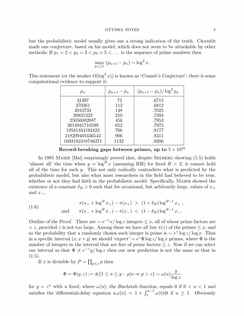
but the probabilistic model usually gives one a strong indication of the truth. Cramermade one conjecture, based on his model, which does not seem to be attackable by othermethods: If p1 = 2 < p2 = 3 < p3 = 5 < . . . is the sequence of prime numbers then
maxpn≤x
(pn+1 − pn) ∼ log2 x.
This statement (or the weaker O(log2 x)) is known as ‘Cramer’s Conjecture’; there is somecomputational evidence to support it:
pn pn+1 − pn (pn+1 − pn)/ log2 pn
31397 72 .6715370261 112 .68122010733 148 .702520831323 210 .7394
25056082087 456 .79532614941710599 652 .797519581334192423 766 .8177218209405436543 906 .83111693182318746371 1132 .9206
Record-breaking gaps between primes, up to 5× 10¹⁶
In 1985 Maier [Mai] surprisingly proved that, despite Selberg showing (1.5) holds‘almost all’ the time when y = logB x (assuming RH) for fixed B > 2, it cannot holdall of the time for such y. This not only radically contradicts what is predicted by theprobabilistic model, but also what most researchers in the field had believed to be true,whether or not they had faith in the probabilistic model. Specifically, Maier showed theexistence of a constant δB > 0 such that for occasional, but arbitrarily large, values of x+
and x−,
(1.6)π(x+ + logB x+)− π(x+) > (1 + δB) logB−1 x+ ,
and π(x− + logB x−)− π(x−) < (1− δB) logB−1 x−.
Outline of the Proof. There are ∼ e−γx/ log z integers ≤ x, all of whose prime factors are> z, provided z is not too large. Among these we have all but π(z) of the primes ≤ x, andso the probability that a randomly chosen such integer is prime is ∼ eγ log z/ log x. Thusin a specific interval (x, x + y] we should ‘expect’ ∼ eγΦ log z/ log x primes, where Φ is thenumber of integers in the interval that are free of prime factors ≤ z. Now if we can selectour interval so that Φ 6∼ e−γy/ log z then our new prediction is not the same as that in(1.5).
If x is divisible by P =∏
p≤z p then
Φ = Φ(y, z) := #1 ≤ n ≤ y : p|n ⇒ p > z ∼ ω(u)y
log z
for y = zu with u fixed, where ω(u), the Buchstab function, equals 0 if 0 < u < 1 andsatisfies the differential-delay equation uω(u) = 1 +
∫ u−1
1ω(t)dt if u ≥ 1. Obviously
6 ANDREW GRANVILLE
limu→∞ ω(u) = e−γ . Iwaniec showed that ω(u)− e−γ oscillates, crossing zero either onceor twice in every interval of length 1. Thus if we fix u > B, chosen so that ω(u) > e−γ or< e−γ (as befits the case of (1.6)), select y = logB x and z = y1/u, and ‘adjust’ x so thatit is divisible by P , then we expect (1.5) to be false.
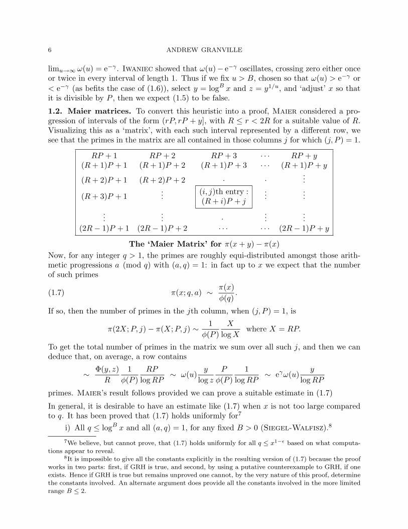
1.2. Maier matrices. To convert this heuristic into a proof, Maier considered a pro-gression of intervals of the form (rP, rP + y], with R ≤ r < 2R for a suitable value of R.Visualizing this as a ‘matrix’, with each such interval represented by a different row, wesee that the primes in the matrix are all contained in those columns j for which (j, P ) = 1.
RP + 1 RP + 2 RP + 3 · · · RP + y(R + 1)P + 1 (R + 1)P + 2 (R + 1)P + 3 · · · (R + 1)P + y
(R + 2)P + 1 (R + 2)P + 2 · · ...
(R + 3)P + 1... (i, j)th entry :
(R + i)P + j
......
...... · ...
...(2R− 1)P + 1 (2R− 1)P + 2 · · · · · · (2R− 1)P + y
The ‘Maier Matrix’ for π(x + y)− π(x)Now, for any integer q > 1, the primes are roughly equi-distributed amongst those arith-metic progressions a (mod q) with (a, q) = 1: in fact up to x we expect that the numberof such primes
(1.7) π(x; q, a) ∼ π(x)φ(q)
.
If so, then the number of primes in the jth column, when (j, P ) = 1, is
π(2X;P, j)− π(X; P, j) ∼ 1φ(P )
X
log Xwhere X = RP.
To get the total number of primes in the matrix we sum over all such j, and then we candeduce that, on average, a row contains
∼ Φ(y, z)R
1φ(P )
RP
log RP∼ ω(u)
y
log z
P
φ(P )1
log RP∼ eγω(u)
y
log RP
primes. Maier’s result follows provided we can prove a suitable estimate in (1.7)
In general, it is desirable to have an estimate like (1.7) when x is not too large comparedto q. It has been proved that (1.7) holds uniformly for7
i) All q ≤ logB x and all (a, q) = 1, for any fixed B > 0 (Siegel-Walfisz).8
7We believe, but cannot prove, that (1.7) holds uniformly for all q ≤ x1−ε based on what computa-tions appear to reveal.
8It is impossible to give all the constants explicitly in the resulting version of (1.7) because the proofworks in two parts: first, if GRH is true, and second, by using a putative counterexample to GRH, if oneexists. Hence if GRH is true but remains unproved one cannot, by the very nature of this proof, determinethe constants involved. An alternate argument does provide all the constants involved in the more limitedrange B ≤ 2.
OTTAWA NOTES 7
ii) All q ≤ √x/ log2+ε x and all (a, q) = 1, assuming GRH9. In fact (1.7) then holds
with error term O(√
x log2(qx)).
iii) Almost all q ≤ √x/ log2+ε x and all (a, q) = 1 (Bombieri-Vinogradov)10.
iv) Almost all q ≤ x1/2+o(1) with (q, a) = 1, for fixed a 6= 0 (Bombieri-Friedlander-Iwaniec, Fouvry)
v) Almost all q ≤ x/ log2+ε x and almost all (a, q) = 1 (Barban-Davenport-Halberstam, Montgomery, Hooley).
Thus, when GRH is true, we get a good enough estimate in (1.7) with R = P 2 to completeMaier’s proof. However Maier, in the spirit of the Bombieri-Vinogradov Theorem,showed how to pick a ‘good’ value for P , so that (1.7) is off by, at worst, an insignificantfactor when R is a large, but fixed, power of P (thus proving his result unconditionally).
In [GS7], we extended the range for y in the proof above, establishing that thereare intervals (x, x + y] in every interval [X, 2X] for which (1.4) fails to hold for somey > exp
(c(log x/ log log x)1/2
).
It is plausible that (1.5) holds uniformly if log y/ log log x → ∞ as x → ∞; and that(1.4) holds uniformly for T = P if y > exp
((log x)1/2+ε
)(at least, we can’t disprove these
statements as yet). We conjecture, presumably safely, that (1.4) and (1.5) hold uniformlywhen y > xε.
One can show that there are more than x/ exp ((log x)cB ) integers x± ≤ x satisfyingthe unexpected inequalities in (1.6).
Maier’s work suggests that Cramer’s model should be adjusted to take into accountdivisibility of n by ‘small’ primes11. It is plausible to define ‘small’ to mean those primesup to a fixed power of log n. Then we are led to conjecture that there are infinitelymany primes pn with pn+1 − pn > 2e−γ log2 pn, contradicting Cramer’s conjecture, as2e−γ > 1.12
If we analyze the distribution of primes in arithmetic progressions using a suitableanalogue of Cramer’s model, then we would expect (1.7), and even
(1.7′) π(x; q, a) =π(x)φ(q)
+ O
((x
q
)1/2
log(qx)
),
to hold uniformly when (a, q) = 1 in the range
(1.8) q ≤ Q = x/ logB x ,
for any fixed B > 2. However the method of Maier is easily adapted to show thatneither (1.7) nor (1.7′) cannot hold in at least part of the range (1.8): For any fixed
9The Generalized Riemann Hypothesis (GRH) states that if β+iγ is a zero of any Dirichlet L-functionthen β ≤ 1/2
10This result is often referred to as ‘GRH on average’. See section 6.4 for another result of this type.11One has to be careful about the meaning of ‘small’ here, since if we were to take into account the
divisibility of n by all primes up to√
n, then we would conclude that there are ∼ e−γx/ log x primes upto x.
12It is unclear what the ‘correct conjecture’ here should be since, to get at it with this approach, wewould need more precise information on ‘sifting limits’ than is currently available.

8 ANDREW GRANVILLE
B > 0 there exists a constant δB > 0 such that for any modulus q, with ‘not too manysmall prime factors’, there exist arithmetic progressions a± (mod q) and values x± ∈[φ(q) logB q, 2φ(q) logB q] such that
(1.9) π(x+; q, a+) > (1 + δB)π(x+)φ(q)
and π(x−; q, a−) < (1− δB)π(x−)φ(q)
.
The proof is much as before, though now using a modified ‘Maier matrix’:
RP RP + q RP + 2q · · · RP + yq(R + 1)P (R + 1)P + q (R + 1)P + 2q · · · (R + 1)P + yq
(R + 2)P (R + 2)P + q · · ...
(R + 3)P... (i, j)th entry :
(R + i)P + jq
......
...... · ...
...(2R− 1)P (2R− 1)P + q · · · · · · (2R− 1)P + yq
The Maier Matrix for π(yq; q, a)
The Bombieri-Vinogradov Theorem is usually stated in a stronger form thanabove: For any given A > 0, there exists a value B = B(A) > 0 such that
(1.10)∑
q≤Q
max(a,q)=1
maxy≤x
∣∣∣∣π(y; q, a)− π(y)φ(q)
∣∣∣∣ ¿x
logA x
where Q =√
x/ logB x. It is possible [FG1] to take the same values of R and P in the Maiermatrix above for many different values of q, and thus deduce that there exist arbitrarilylarge values of a and x for which
(1.11)
∣∣∣∣∣∣∣∣
∑
Q≤q≤2Q(q,a)=1
π(x; q, a)− π(x)
φ(q)
∣∣∣∣∣∣∣∣À x;
thus refuting the conjecture that for any given A > 0, (1.10) should hold in the range (1.8)for some B = B(A) > 0. In [FG2] we showed that (1.10) even fails with
Q = x/ exp((A− ε)(log log x)2/(log log log x)
).
In [GS7] we showed that, for any q ≥ x/ exp((log x)1/2−ε
), the bound (1.7′) cannot hold
for every integer a prime to q.It seems plausible that (1.7) holds uniformly if log(x/q)/ log log q → ∞ as q → ∞;
and that (1.10) holds uniformly for Q < x/ exp((log x)1/2+ε
). At least we can’t disprove
OTTAWA NOTES 9
these statements as yet, though we might play it safe and conjecture only that they holduniformly for q, Q < x1−ε.
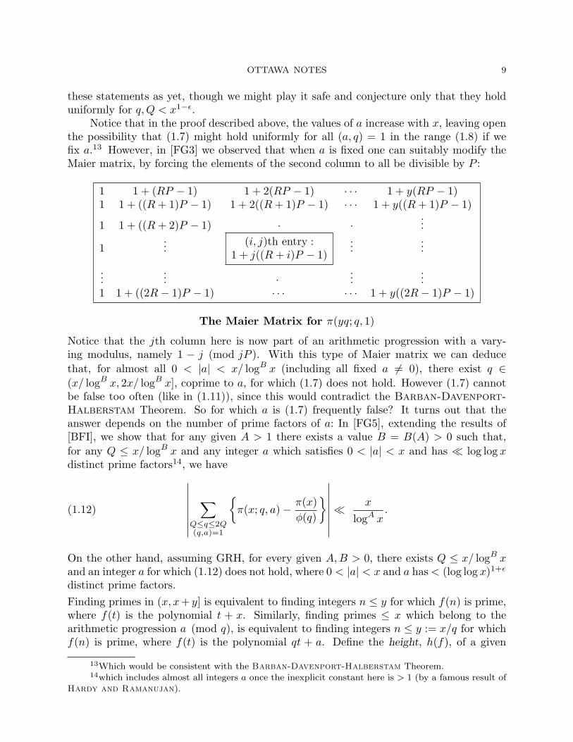
Notice that in the proof described above, the values of a increase with x, leaving openthe possibility that (1.7) might hold uniformly for all (a, q) = 1 in the range (1.8) if wefix a.13 However, in [FG3] we observed that when a is fixed one can suitably modify theMaier matrix, by forcing the elements of the second column to all be divisible by P :
1 1 + (RP − 1) 1 + 2(RP − 1) · · · 1 + y(RP − 1)1 1 + ((R + 1)P − 1) 1 + 2((R + 1)P − 1) · · · 1 + y((R + 1)P − 1)
1 1 + ((R + 2)P − 1) · · ...
1... (i, j)th entry :
1 + j((R + i)P − 1)...
...
...... · ...
...1 1 + ((2R− 1)P − 1) · · · · · · 1 + y((2R− 1)P − 1)
The Maier Matrix for π(yq; q, 1)
Notice that the jth column here is now part of an arithmetic progression with a vary-ing modulus, namely 1 − j (mod jP ). With this type of Maier matrix we can deducethat, for almost all 0 < |a| < x/ logB x (including all fixed a 6= 0), there exist q ∈(x/ logB x, 2x/ logB x], coprime to a, for which (1.7) does not hold. However (1.7) cannotbe false too often (like in (1.11)), since this would contradict the Barban-Davenport-Halberstam Theorem. So for which a is (1.7) frequently false? It turns out that theanswer depends on the number of prime factors of a: In [FG5], extending the results of[BFI], we show that for any given A > 1 there exists a value B = B(A) > 0 such that,for any Q ≤ x/ logB x and any integer a which satisfies 0 < |a| < x and has ¿ log log xdistinct prime factors14, we have
(1.12)
∣∣∣∣∣∣∣∣
∑
Q≤q≤2Q(q,a)=1
π(x; q, a)− π(x)
φ(q)
∣∣∣∣∣∣∣∣¿ x
logA x.
On the other hand, assuming GRH, for every given A, B > 0, there exists Q ≤ x/ logB xand an integer a for which (1.12) does not hold, where 0 < |a| < x and a has < (log log x)1+ε
distinct prime factors.Finding primes in (x, x+ y] is equivalent to finding integers n ≤ y for which f(n) is prime,where f(t) is the polynomial t + x. Similarly, finding primes ≤ x which belong to thearithmetic progression a (mod q), is equivalent to finding integers n ≤ y := x/q for whichf(n) is prime, where f(t) is the polynomial qt + a. Define the height, h(f), of a given
13Which would be consistent with the Barban-Davenport-Halberstam Theorem.14which includes almost all integers a once the inexplicit constant here is > 1 (by a famous result of
Hardy and Ramanujan).

10 ANDREW GRANVILLE
polynomial f(t) =∑
i citi to be h(f) :=
√∑i c2
i . In the cases above, in which the degreeis always 1, we proved that we do not always get the asymptotically expected number ofprime values f(n) with n ≤ y = logB h(f), for any fixed B > 0. In [FG4] we showedthat this is true for polynomials of arbitrary degree d, which is somewhat ironic since it isnot known that any polynomial of degree ≥ 2 takes on infinitely many prime values, northat the prime values are ever ‘well-distributed’. Nair and Perelli [NP] showed thatsome of the polynomials FR(n) = nd + RP attain more than, and others attain less than,the number of prime values expected in such a range, by considering the following Maiermatrix:
FR(1) FR(2) FR(3) · · · FR(y)FR+1(1) FR+1(2) FR+1(3) · · · FR+1(y)
FR+2(1) FR+2(2) · · ...
FR+3(1)... (i, j)th entry :
FR+i(j)...
...
...... · ...
...F2R−1(1) F2R−1(2) · · · · · · F2R−1(y)
The Maier Matrix for πF (y)Notice that the jth column here is part of the arithmetic progression jd (mod P ).
Using Maier matrices it is possible to prove ‘bad equi-distribution’ results for primesin other interesting sequences, such as the values of binary quadratic forms, and of primepairs. For example, if we fix B > 0 then, once x is sufficiently large, there exists a positiveinteger k ≤ log x such that there are at least 1 + δB times as many prime pairs p, p + 2k,with x < p ≤ x+logB x, as we would expect from assuming that the estimate in HypothesisH holds uniformly for n ¿ logB h((t + x)(t + (x + 2k))) .
We have now seen that the asymptotic formula in Hypothesis H fails when x is anarbitrary fixed power of log h(F )(:=
∑i log h(fi)), for many different non-trivial examples
F . Presumably the asymptotic formula does hold uniformly as log x/ log log h(F ) → ∞.However, to be safe, we only make the following prediction:
Conjecture. Fix ε > 0 and positive integer k. The asymptotic formula in Hypothesis Hholds uniformly for x > h(F )ε as h(F ) →∞.
Our work here shows that the ‘random-like’ behaviour exhibited by primes in many situa-tions does not carry over to all situations. It remains to discover a model that will alwaysaccurately predict how primes are distributed, since it seems that minor modifications ofCramer’s model will not do. We thus agree that:
“It is evident that the primes are randomly distributed but, unfortunately,we don’t know what ‘random’ means.” — R.C. Vaughan (February 1990).
1.3. And beyond. Armed with Maier’s ideas it seems possible to construct incorrectconclusions from, more-or-less, any variant of Cramer’s model. This flawed model maystill be used to make conjectures about the distribution of primes, but one should be verycautious of such predictions!

OTTAWA NOTES 11
There are no more than O(x2/ log3B x) arithmetic progressions a (mod q), with 1 ≤a < q < x/ logB x and (a, q) = 1, for which (1.7) fails, by the Barban-Davenport-Halberstam Theorem. However our methods here may be used to show that (1.7) doesfail for more than x2/ exp ((log x)ε) such arithmetic progressions.
Maier’s matrix has been used in other problems too: Konyagin used it to find un-usually large gaps between consecutive primes. Maier used it to find long sequences ofconsecutive primes, in which there are longer than average gaps between each pair. Shiuhas used it to show that every arithmetic progression a (mod q) with (a, q) = 1 containsarbitrarily long strings of consecutive primes. Recently Thorne15 generalized these ideasto function fields, and to Gaussian primes.
Despite the efforts of several mathematicians we have still not got a particularly goodmodel to replace the now discredited model of Cramer. Certainly not a well-motivatedone, so there are still many questions about the distribution of primes in which we cannoteven guess at the right answer with much confidence. This is not a new complaint:
“Mathematicians have tried in vain to discover some order in the sequenceof prime numbers but we have every reason to believe that there are some
mysteries which the human mind will never penetrate.”
— L. Euler (1770).
2. The Uncertainty Principle, in the twenty-first century
2.1. A general phenomenon. I ended my 1994 ICM talk with Euler’s quote – itseemed fitting since these counterintuitive extensions of Maier’s results seemed to besomething to do with Euler’s observation that primes refuse, in almost every way, to beeasily understood. There was a hiatus in developments in this subject, until a paper ofBalog and Wooley [BW] appeared in 2000. There they applied the same circle of ideasto the integers that are the sum of two squares, and proved an analogous result to that ofMaier. My first reaction when I heard about their work was that it was nice they hadgeneralized things beyond primes, but was this really so interesting? Especially as it wasprobably technically easier than Maier’s work on primes? They sent me a reprint of theirpaper and it sat unread on my desk for an embarrassingly long time. After two years Ipicked it up and almost immediately realized that what they had done was a big surpriseand their work surely pointed the way to an important phenomenon . . . The point is that Ihad thought that irregularities in the distribution of primes came about because primes arealways “strange”, but here Balog and Wooley had taken a relatively civilized sequence,one with very predictable multiplicative structure even, and found similar irregularities inthe distribution. This meant that Maier’s proof was surely nothing to do with primesand must be the harbinger of a much more general phenomenon. Indeed this intuition wascorrect and Sound and I were able to prove a very general “uncertainty principle” whichestablishes that most arithmetic sequences of interest are either not-so-well distributed inlongish arithmetic progressions, or are not-so-well distributed in both short intervals andshort arithmetic progressions.
15In his 2008 Ph.D. at Madison.

12 ANDREW GRANVILLE
With probability 1, there are no “Maier-type” irregularities in the distribution ofrandomly chosen subsets of the integers. Indeed such irregularities seem to depend onour sequence coming from arithmetic. Sieve theory already provides a framework forconsidering analytic properties of “arithmetic sequences”, so this is our starting point:
A could be a set of integers but, more generally, let A denote a sequence a(n) ofnon-negative real numbers, and A(x) =
∑n≤x a(n). If the a(n) are well-distributed in
short intervals then we expect
(2.1) A(x + y)−A(x) ≈ yA(x)
x,
for suitable y.Suppose that the proportion of A which is divisible by d is approximately h(d)/d
where h(.) is a non-negative multiplicative function; in other words,
(2.2) Ad(x) :=∑
n≤xd|n
a(n) ≈ h(d)dA(x),
for each d.16 The reason for taking h(d) to be a multiplicative function is that for mostsequences that appear in arithmetic one expects that the criterion of being divisible byan integer d1 should be “independent” of the criterion of being divisible by any integer d2
which is coprime with d1.If the asymptotic behavior of A in the arithmetic progression a (mod q), depends only
on (a, q) when (q,S) = 1 then, by (2.2), we arrive at the prediction that, for (q,S) = 1,
(2.3) A(x; q, a) :=∑
n≤xn≡a (mod q)
a(n) ≈ fq(a)qγq
A(x),
where γq =∏
p|q((p − 1)/(p − h(p))) and fq(a) is a certain non-negative multiplicativefunction of a for which fq(a) = fq((a, q)) (thus fq(a) is periodic (mod q)).17
Example 1. We take a(n) = 1 for all n, so that h(n) = 1 for all n. Then fq(a) = 1 forall q and all a, and γq = 1. Clearly both (2.3) and (2.1) are good approximations with anerror of at most 1.Example 2. We take a(n) = 1 if n is prime and a(n) = 0 otherwise, so that h(n) = 1 ifn = 1 and h(n) = 0 if n > 1. Further fq(a) = 1 if (a, q) = 1 and fq(a) = 0 otherwise, andγq = φ(q)/q. The approximation (2.3) is then the prime number theorem for arithmeticprogressions for small q ≤ (log x)A. Friedlander and Granville’s result (1.1) setslimitations to (2.3), and Maier’s result sets limitations to (2.1).Example 3. Take a(n) = 1 if n is the sum of two squares and a(n) = 0 otherwise. Herewe take S = 2, and for odd prime powers pk we have h(pk) = 1 if pk ≡ 1 (mod 4) andh(pk) = 1/p otherwise. Balog and Wooley’s result places restrictions on the validityof (2.1).
A weak form of our main results are given in the next two Theorems:
16Or perhaps when (d,S) = 1, where S is a finite set of ‘bad’ primes.17We prove this in section 2.2 below, giving an explicit description of fq in terms of h.
OTTAWA NOTES 13
Theorem 2.1. Let A, S, h, fq and γq be as above. For given α > 0 there exist constantsc′ > 0, c > 1 such that, for sufficiently large x, if either
(2.4)∑
p≤log x
max0, 1− h(p)p
log p ≥ α log log x,
or there exists n ≤ x with h(n) ≥ (log x)c′ , and if 1 ¿ u ¿ (log x)c′ then there existsy ∈ (x/4, x) and an arithmetic progression a (mod `) with ` ≤ x/(log x)u and (`,S) = 1such that ∣∣∣A(y; `, a)− f`(a)
`γ`yA(x)
x
∣∣∣ À u−cuA(x)φ(`)
.
The condition (2.4) ensures that h(p) is not always close to 1; this is essential in orderto eliminate the very well behaved Example 1.
One can show that A(x)φ(`) ≥ 1
`γ`yA(x)
x . It is good to not have f`(a) in the lower boundsince it may well be 0.
Theorem 2.1 applies to the sequences of primes (with α = 1 + o(1)) and sums of twosquares (with α = 1/2 + o(1)), two results already known. Surprisingly it also applies toany subset of the primes:Example 4. Let A be any subset of the primes. Fix u ≥ 1. For any x there existsy ∈ (x/4, x) such that either
(2.5a) |A(y)/y −A(x)/x| Àu A(x)/x
(meaning that the subset is poorly distributed in short intervals), or there exists somearithmetic progression a (mod `) with (a, `) = 1 and ` ≤ x/(log x)u, for which
(2.5b)∣∣∣A(y; `, a)− A(y)
φ(`)
∣∣∣ ÀuA(x)φ(`)
.
In other words, we find “Maier type” irregularities in the distribution of any subset ofthe primes.18 A similar result holds for any subset of the numbers that are sums of twosquares.
Let Sε be the set of integers n having no prime factors in the interval [(log n)1−ε, log n],so that Sε(N) ∼ (1 − ε)N . Notice that the primes are a subset of Sε. Theorem 2.1 withα ≥ ε + o(1) implies that any subset A of Sε is poorly distributed in that for any x thereexists y ∈ (x/4, x) such that either (2.5a) holds, or there exists some arithmetic progressiona (mod `) and ` ≤ x/(log x)u with (a, `) = 1, for which a suitably modified (2.5b) holds(that is with φ(`) replaced by `
∏p|`, (log x)1−ε<p<log x(1− 1/p)).
Our next result gives an “uncertainty principle” implying that we either have poordistribution in long arithmetic progressions, or in short intervals, generalizing Maier’soriginal result:.
18If we had chosen A to be the primes ≡ 5 (mod 7) then this is of no interest when we take a =1, ` = 7. To avoid this minor technicality we can add “For a given finite set of “bad primes” S, we canchoose such an ` for which (`,S) = 1”, where (`,S) = 1 means that (`, p) = 1 for all p ∈ S.

14 ANDREW GRANVILLE
Theorem 2.2. Let A, S, h, fq and γq be as above. For given α > 0 there exist constantsc′ > 0, c > 1 such that, for sufficiently large x, if either (2.4) holds or there exists n ≤ x
with h(n) ≥ (log x)c′ , and if 1 ¿ u ¿ (log x)c′ then at least one of the following twoassertions holds:
(i) There exists an interval (v, v + y) ⊂ (x/4, x) with y ≥ (log x)u such that∣∣∣A(v + y)−A(v)− y
A(x)x
∣∣∣ À u−cuyA(x)
x.
(ii) There exists y ∈ (x/4, x) and an arithmetic progression a (mod q) with (q,S) = 1and q ≤ exp(2(log x)1−η) such that
∣∣∣A(y; q, a)− fq(a)qγq
yA(x)
x
∣∣∣ À u−cuA(x)φ(q)
.
This is aptly named an “uncertainty principle” for we can construct sequences whichare well distributed in short intervals (and then must have fluctuations in arithmetic pro-gressions), and primes are known to be well-distributed in these long arithmetic progres-sions (and so exhibit fluctuations in short intervals).
Our proofs develop Maier’s “matrix method”: In the earlier work on primes andsums of two squares, the problem then reduced to showing oscillations in certain siftingfunctions arising from the theory of the half dimensional (for sums of two squares) andlinear (for primes) sieves. In our case the problem boils down to proving oscillations in themean-value of the more general class of multiplicative functions satisfying 0 ≤ f(n) ≤ 1for all n (as we will discuss in section 2.3). In section 3.4 we will prove an analogy of suchoscillation results for a wide class of related integral equations, which has the flavor of aclassical “uncertainty principle” from Fourier analysis (and hence the nomenclature).
2.2. The new framework. We may assume that h(pk) < pk for all prime powers pk
without any significant loss of generality.We hypothesize that, for (q,S) = 1, the asymptotics of A(x; q, a) depends only on the
greatest common divisor of a and q. Writing (q, a) = m, since |b (mod q) : (b, q) = m| =ϕ(q/m), we then guess that
A(x; q, a) ≈ 1ϕ(q/m)
∑
n≤x(q,n)=m
a(n) =1
ϕ(q/m)
∑
n≤xm|n
a(n)∑
d| qm
d| nm
µ(d) =1
ϕ(q/m)
∑
d| qm
µ(d)Adm(x).
Using now (2.2) we would guess that
(2.6) A(x; q, a) ≈ A(x)1
ϕ(q/m)
∑
d| qm
µ(d)h(dm)
dm=:
fq(a)qγq
A(x),
where
(2.7) γq =∏
p|q
(1− h(p)/p
1− 1/p
)−1
=∏p
(1− 1
p
)(1 +
fq(p)p
+fq(p2)
p2+ . . .
),

OTTAWA NOTES 15
and fq(a), a multiplicative function with fq(a) = fq((a, q)) so that it has period q, isdefined as follows: fq(pk) = 1 if p - q. If p divides q, indeed if pe is the highest power of pdividing q then
fq(pk) :=
(h(pk)− h(pk+1)
p
)(1− h(p)
p
)−1
if k < e
h(pe)(1− 1
p
)(1− h(p)
p
)−1
if k ≥ e.
Note that if q is squarefree and h(p) ≤ 1 then fq(pk) ≤ 1 for all prime powers pk.
We may assume that 0 ≤ h(n) ≤ 1 for all n, since such results are easy if h(p) > 1often:19
Proposition 2.3. Suppose that q ≤ x is an integer for which h(q) > 6. Then either20
∣∣∣A(x; q, 0)− fq(0)qγq
A(x)∣∣∣ ≥ 1
2fq(0)qγq
A(x)
or, for every prime ` in the range x ≥ ` ≥ 3(x + q)/h(q) which does not divide q, there isan arithmetic progression b (mod `) such that
∣∣∣A(x; `, b)− f`(b)`γ`
A(x)∣∣∣ ≥ 1
2f`(b)`γ`
A(x).
Proof. If the first option fails then
∑
n≤x/q
A(x; `, nq) ≥∑
n≤x/q
a(nq) = A(x; q, 0) ≥ 12
fq(0)qγq
A(x) =h(q)2q
A(x).
On the other hand, if prime ` - q then f`(nq) = 1 if ` - n, and f`(nq) = h(`)γ` if `|n.Therefore for any N ,
∑
n≤N
f`(nq)`γ`
=∑
n≤Nl-n
1`γ`
+∑
n≤Nl|n
h(`)`
=1
`− 1([N ]− [N/`])− h(`)
`(`− 1)(`N/` − N) ≤ N + 1
`.
Combining this (taking N = x/q) with the display above yields
∑
n≤x/q
A(x; `, nq) ≥ h(q)2q
A(x) ≥ 3(x + q)2q`
A(x) ≥ 32
∑
n≤x/q
f`(nq)`γ`
A(x),
19Proposition 2.3 implies Theorems 2.1 and 2.2 when there exists n ≤ x with h(n) ≥ (log x)c′ .20Note that this criterion is equivalent to |Aq(x)−(h(q)/q)A(x)| ≥ 1
2(h(q)/q)A(x), since fq(0)/qγq =
fq(q)/qγq = h(q)/q.
16 ANDREW GRANVILLE
which implies the Proposition with b = nq for some n ≤ x/q.
From now on assume 0 ≤ h(n) ≤ 1 for all n. Suppose that (q,S) = 1 and define∆q = ∆q(x) by
(2.8) ∆q(x) := maxx/4≤y≤x
maxa (mod q)
∣∣∣A(y; q, a)− fq(a)qγq
y
xA(x)
∣∣∣/ A(x)
φ(q).
We can now formulate our main principle.
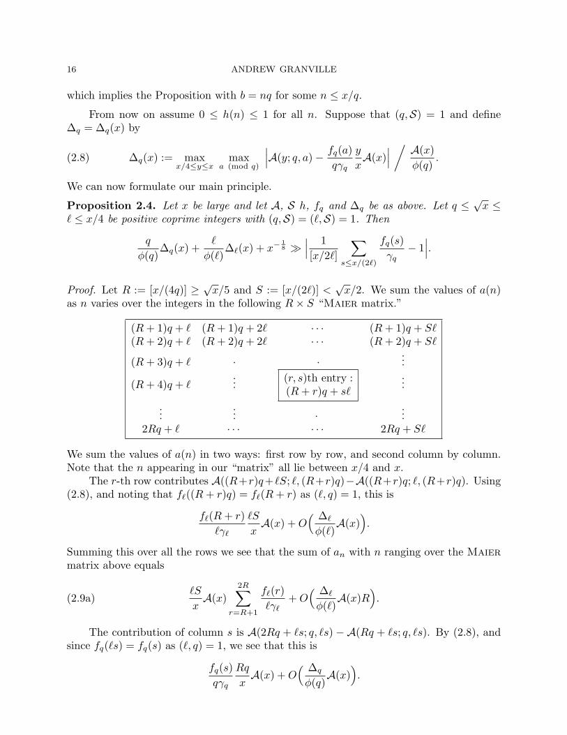
Proposition 2.4. Let x be large and let A, S h, fq and ∆q be as above. Let q ≤ √x ≤
` ≤ x/4 be positive coprime integers with (q,S) = (`,S) = 1. Then
q
φ(q)∆q(x) +
`
φ(`)∆`(x) + x−
18 À
∣∣∣ 1[x/2`]
∑
s≤x/(2`)
fq(s)γq
− 1∣∣∣.
Proof. Let R := [x/(4q)] ≥ √x/5 and S := [x/(2`)] <
√x/2. We sum the values of a(n)
as n varies over the integers in the following R× S “Maier matrix.”
(R + 1)q + ` (R + 1)q + 2` · · · (R + 1)q + S`(R + 2)q + ` (R + 2)q + 2` · · · (R + 2)q + S`
(R + 3)q + ` · · ...
(R + 4)q + `... (r, s)th entry :
(R + r)q + s`
...
...... · ...
2Rq + ` · · · · · · 2Rq + S`
We sum the values of a(n) in two ways: first row by row, and second column by column.Note that the n appearing in our “matrix” all lie between x/4 and x.
The r-th row contributes A((R+r)q+`S; `, (R+r)q)−A((R+r)q; `, (R+r)q). Using(2.8), and noting that f`((R + r)q) = f`(R + r) as (`, q) = 1, this is
f`(R + r)`γ`
`S
xA(x) + O
( ∆`
φ(`)A(x)
).
Summing this over all the rows we see that the sum of an with n ranging over the Maiermatrix above equals
(2.9a)`S
xA(x)
2R∑
r=R+1
f`(r)`γ`
+ O( ∆`
φ(`)A(x)R
).
The contribution of column s is A(2Rq + `s; q, `s) −A(Rq + `s; q, `s). By (2.8), andsince fq(`s) = fq(s) as (`, q) = 1, we see that this is
fq(s)qγq
Rq
xA(x) + O
( ∆q
φ(q)A(x)
).

OTTAWA NOTES 17
Summing this over all the columns we see that the Maier matrix sum is
(2.9b)Rq
xA(x)
S∑s=1
fq(s)qγq
+ O( ∆q
φ(q)A(x)S
).
Comparing (2.9a) and (2.9b) we deduce that
(2.10)1
Sγq
S∑s=1
fq(s) + O( q∆q
φ(q)
)=
1Rγ`
2R∑
r=R+1
f`(r) + O( `∆`
φ(`)
).
Write f`(r) =∑
d|r g`(d) for a multiplicative function g`. Note that g`(pk) = 0 ifp - `. We also check easily that |g`(pk)| ≤ (p + 1)/(p − 1) for primes p|`, and note thatγ` =
∑∞d=1 g`(d)/d. Thus
1Rγ`
2R∑
r=R+1
f`(r) =1
Rγ`
∑
d≤2R
g`(d)(R
d+O(1)
)= 1+O
( 1γ`
∑
d>2R
|g`(d)|d
+1
Rγ`
∑
d≤2R
|g`(d)|).
We see easily that the error terms above are bounded by
¿ 1R
13 γ`
∞∑
d=1
|g`(d)|d
23
¿ 1R
13
∏
p|`
(1 + O
( 1p
23
))¿ 1
R14,
since ` ≤ x, and R À √x. We conclude that
1Rγ`
2R∑
r=R+1
f`(r) = 1 + O(R−14 ).
Combining this with (2.10) we obtain the Proposition.
In Proposition 2.4 we compared the distribution of A in two arithmetic progressions.We may also compare the distribution of A in an arithmetic progression versus the distri-bution in short intervals. Define ∆(y) = ∆(y, x) by
(2.11) ∆(y, x) := max(v,v+y)⊂(x/4,x)
∣∣∣A(v + y)−A(v)− yA(x)
x
∣∣∣/
yA(x)
x.
Proposition 2.5. Let x be large and let A, S, h, fq, ∆q and ∆ be as above. Let q ≤ √x
with (q,S) = 1 and let y ≤ x/4 be positive integers. Then
q
φ(q)∆q(x) + ∆(x, y) À
∣∣∣ 1γqy
∑
s≤y
fq(s)− 1∣∣∣.
Proof. The argument is similar to the proof of Proposition 2.4, starting with an R × y“Maier matrix” (again R = [x/(4q)]) whose (r, s)-th entry is (R + r)q + s. We omit thedetails.

18 ANDREW GRANVILLE
2.3. Oscillations in mean-values of multiplicative functions. Assume that q isan integer all of whose prime factors are less than or equal to large z. Let fq(n) be amultiplicative function with fq(pk) = 1 for all p - q, and 0 ≤ fq(n) ≤ 1 for all n. Note thatfq(n) = fq((n, q)) is periodic (mod q). Define
Fq(s) =∞∑
n=1
fq(n)ns
= ζ(s)Gq(s), where Gq(s) =∏
p|q
(1− 1
ps
)(1+
fq(p)ps
+fq(p2)p2s
+. . .).
To start with, Fq is defined in Re(s) > 1, but the above furnishes a meromorphic continu-ation to Re(s) > 0. Now γq = Gq(1), and define
E(u) :=1zu
∑
n≤zu
(fq(n)−Gq(1)),
which is what we need to consider in Propositions 2.2 and 2.3 above. For complex numberξ, let H(ξ) := H0(ξ) where
Hj(ξ) :=∑
p|q
1− fq(p)p1−ξ/ log z
( log(z/p)log z
)j
for each j ≥ 0, and J(ξ) :=∑
p|q
1p2(1−ξ/ log z)
.
One can easily show that for π ≤ ξ ≤ 23 log z one has
|E(u)| ≤ exp(H(ξ)− ξu + 5J(ξ)).
The new development is to show that if
τ :=√
(5H2(ξ) + 19J(ξ) + 5)/H(ξ) ≤ 1/2
then there exist points u± in the interval [H(ξ)(1− 2τ), H(ξ)(1 + 2τ)] such that
±E(u±) ≥ 120ξH(ξ)
expH(ξ)− ξu± − 5H2(ξ)− 5J(ξ).
This gives us, in some generality, a best possible oscillation result up to a small factor. Wewill not prove this result here, but we will later (in section 3.4) indicate how we proved it,though first (in section 3) we will need to discuss the theory of mean values of multiplicativefunctions in some detail.
By a judicious choice of ξ, one can deduce Theorems 2.1 and 2.2 from Propositions2.4 and 2.5 respectively.
2.4. More Examples.
• Sieves. Let B be a given set of x integers and P be a given set of primes. DefineS(B,P, z) to be the number of integers in B which do not have a prime factor p ∈ Pwith p ≤ z. Sieve theory is concerned with estimating S(B,P, z) under certain natural

OTTAWA NOTES 19
hypothesis for B,P and u := log x/ log z. The fundamental lemma of sieve theory (see[HR1]) implies (for example, when B is the set of integers in an interval) that
∣∣∣∣∣∣S(B,P, z)− x
∏
p∈P,p≤z
(1− 1
p
)∣∣∣∣∣∣¿
(1 + o(1)u log u
)u
x∏
p∈P,p≤z
(1− 1
p
)
for u < z1/2+o(1). It is known that this result is essentially “best-possible” in that one canconstruct examples for which the bound is obtained (both as an upper and lower bound).However these bounds are obtained in quite special examples, and one might suspect thatin many cases which one encounters, those bounds might be significantly sharpened. Itturns out that these bounds cannot be improved for intervals B, when P contains at leasta positive proportion of the primes: We proved in [GS7] that if P is a given set of primesfor which #p ∈ P : p ≤ y À π(y) for all y ∈ (
√z, z], then there exists a constant c > 0
such that for any u ¿ √z there exist intervals I± of length ≥ zu for which
S(I+,P, z) ≥
1 +(
c
u log u
)u|I+|
∏
p∈P,p≤z
(1− 1
p
)
and S(I−,P, z) ≤
1−(
c
u log u
)u|I−|
∏
p∈P,p≤z
(1− 1
p
).
Moreover if u ≤ (1− o(1)) log log z/ log log log z then our intervals I± have length ≤ zu+2.The reduced residues (mod q) are expected to be distributed much like random
numbers chosen with probability φ(q)/q. Indeed when φ(q)/q → 0 this follows fromwork of Hooley, and of Montgomery and Vaughan [MV2] who showed that #n ∈[m,m + h) : (n, q) = 1 has Gaussian distribution with mean and variance equal tohφ(q)/q, as m varies over the integers, provided h is suitably large. This suggests that#n ∈ [m, m + h) : (n, q) = 1 should be 1 + o(1)(hφ(q)/q) provided h ≥ log2 q. How-ever, by a modification of our argument, we can show that this is not true for h = logA qfor any given A > 0, provided that
∑p|q(log p)/p À log log q (a condition satisfied by many
highly composite q). In fact Montgomery and Vaughan showed that
∑
m≤k
( ∑
mh+1≤n≤(m+1)h(n,q)=1
1− φ(q)q
h)2r
∼ (2r)!2rr!
q(h
φ(q)q
)r
for integers r ≥ 1. Our work places restrictions on the uniformity with which this estimatecan hold: Given h and q with hφ(q)/q large, define η by q/φ(q) = (hφ(q)/q)η. If the aboveholds then r ¿ (log(hφ(q)/q))2+4η+o(1).
• Wirsing Sequences. Let P be a set of primes of logarithmic density α for a fixednumber α ∈ (0, 1); that is ∑
p≤xp∈P
log p
p= (α + o(1)) log x,
20 ANDREW GRANVILLE
as x → ∞. Let A be the set of integers not divisible by any prime in P and let a(n) = 1if n ∈ A and a(n) = 0 otherwise. Wirsing proved that (see page 417 of [Ten])
(2.12) A(x) ∼ eγα
Γ(1− α)x
∏
p≤xp∈P
(1− 1
p
).
We can show oscillatory results for any such A: Fix u ≥ max(e2/α, e100) and suppose x issufficiently large. Then there exists y ∈ (x/4, x) and an arithmetic progression a (mod `)with ` ≤ x(3/ log x)u such that
∣∣∣A(y; `, a)− f`(a)`γ`
A(y)∣∣∣ À exp(−u(log u + O(log log u)))
A(y)φ(`)
.
Moreover suppose MN = u with M, N ≥ 1. Then at least one of the following is true:Either there exists y ∈ (x/4, x) and an arithmetic progression a (mod q) with
q ≤ exp((log x)1
M ) such that
∣∣∣A(y; q, a)− fq(a)qγq
A(y)∣∣∣ À exp(−u(log u + O(log log u)))
A(y)φ(q)
.
Or there exists y > ( 13 log x)N and an interval (v, v + y) ⊂ (x/4, x) such that
∣∣∣A(v + y)−A(v)− yA(v)
v
∣∣∣ À exp(−u(log u + O(log log u)))yA(v)
v.
Examples of Wirsing sequences include sums of two squares, in fact norms of integral idealsbelonging to a given ideal class (in a given number field).
3. Halasz’s theorem
3.1. The Halasz-Montgomery theorem. Given a multiplicative function f with|f(n)| ≤ 1 for all n, define
Θ(f, x) :=∏
p≤x
(1 +
f(p)p
+f(p2)
p2+ . . .
)(1− 1
p
).
We are concerned with understanding the mean value of f up to x, that is 1x
∑n≤x f(n).
For real-valued f it turns out that
(3.1a)1x
∑
n≤x
f(n) → Θ(f,∞) as x →∞.
In 1944 Wintner proved this when Θ(f,∞) 6= 0, which is equivalent to the hypothesisthat
∑p(1− f(p))/p converges. In 1967, Wirsing [Wrs] settled the harder remaining case

OTTAWA NOTES 21
when Θ(f,∞) = 0, thereby establishing an old conjecture of Erdos and Wintner thatevery multiplicative function f with −1 ≤ f(n) ≤ 1 has a mean-value.
On the other hand not all complex valued multiplicative functions have a meanvalue tending to a limit; for example, the function f(n) = niα, with α ∈ R \ 0, since1x
∑n≤x niα ∼ xiα/(1+ iα). In the early seventies, Gabor Halasz [Hal1, Hal2] brilliantly
realized that the correct question to ask is whether∑
p(1−Re(f(p)p−iα))/p converges forall real numbers α. His fundamental result states:(I) If
∑p(1− Re(f(p)/piα))/p diverges for all α then 1
x
∑n≤x f(n) → 0 as x →∞.
(II) If there exists α for which∑
p(1− Re(f(p)/piα))/p converges then
(3.1b)1x
∑
n≤x
f(n) ∼ xiα
1 + iαΘ(fα, x)
where fα(n) := f(n)/niα. Now |Θ(fα, x)| → |Θ(fα,∞)| as x → ∞ so we can rewrite theabove as
1x
∑
n≤x
f(n) ∼ xiα
1 + iα|Θ(fα,∞)|eir(x)
where r(x) = arg Θ(fα, x) (which varies very slowly, for example r(x2) = r(x) + o(1)).Also note that if
∑p |1− f(p)/piα|/p converges then (II) holds and Θ(fα, x) → Θ(fα,∞)
as x →∞.Moreover one should note the Corollary that if (II) holds then for any real number β
one has1x
∑
n≤x
f(n)niβ ∼ xi(α+β)
1 + i(α + β)Θ(fα, x).
In case (I), Halasz also quantified how rapidly the limit is attained. His method wasmodified and refined by Montgomery [Mon], Tenenbaum [Ten, p.343], and Sound andI [GS4]: Throughout define
(3.2) M(x, T ) := min|y|≤2T
∑
p≤x
1− Re(f(p)p−iy)p
.
Theorem (Halasz-Montgomery). Let f be a multiplicative function with |f(n)| ≤ 1for all n. Let x ≥ 3 and T ≥ 1 be real numbers, and let M = M(x, T ). If f is completelymultiplicative then
1x
∣∣∣∑
n≤x
f(n)∣∣∣ ≤
(M +
127
)eγ−M + O
( 1T
+log log x
log x
).
If f is multiplicative then
1x
∣∣∣∑
n≤x
f(n)∣∣∣ ≤
∏p
(1 +
2p(p− 1)
)(M +
47
)eγ−M + O
( 1T
+log log x
log x
).

22 ANDREW GRANVILLE
This is essentially “best possible” (up to a factor 10) in that for any given suffi-ciently large m0, we can construct f and x such that M = M(x,∞) = m0 + O(1) and|∑n≤x f(n)| ≥ (M + 12/7)eγ−Mx/10.
If the minimum in (3.2) occurs for y = y0 then one might expect that f(n) looksroughly like niy0 , so that the mean-value of f(n) should be around size |xiy0/(1 + iy0)| ³1/(1 + |y0|). In fact we proved that if the minimum in (3.2) with T = log x is attained aty = y0 then
1x
∣∣∣∑
n≤x
f(n)∣∣∣ ¿ 1
1 + |y0| +(log log x)1+2(1− 2
π )
(log x)1−2π
.
Taking f(n) = niy0 we see that this is best possible in terms of y0 though, in this caseM = 0. Next we proved a hybrid bound between the last two results, obtaining, forM = M(x, log x),
1x
∣∣∣∑
n≤x
f(n)∣∣∣ ¿ (M + 1)
eγ−M
√1 + y2
0
+log log x
(log x)2−√
3.
The right hand side of (3.1b) has size ³ e−M/(1 + |y0|), implying that there is little roomto reduce the bound in Theorem 2b. In fact for any given α and m0 we can determine f ,such that M = m0 + O(1), y0 = α and the bound here is too big by at most a constantfactor.
The minimum in (3.2) can be unwieldy to determine, so it is desirable to get similardecay estimates in terms of
∑p≤x(1 − Re(f(p)))/p (or equivalently |F (1)|). However, in
light of case (II) above, this is only possible if we have some additional information on f ,since the
∑p(1−Re(f(p)))/p may diverge while the absolute value of the mean value may
converge. One can avoid case (II) altogether by insisting that all f(p) lie in some closedconvex subset D of the unit disc U (this is a natural restriction for many applications,such as when f is a Dirichlet character of a given order), as in Halasz [Hal1, Hal2], Halland Tenenbaum [HT], and Hall [Hl2]. The result of Hall is the most general, perhapsqualitatively definitive. To describe it we require some information on the geometry of D:
Throughout we let D be a closed, convex subset of U with 1 ∈ D, and define ν =ν(D) = maxδ∈D(1− Re(δ)). For α ∈ [0, 1] define
(3.3) ~(α) =12π
∫ 2π
0
maxδ∈D
Re((1− δ)(α− e−iθ)) dθ,
which is a continuous, increasing, convex function of α. Note that ~(0) = λ(D)/2π, whereλ(D) is the length of the boundary of D. Define κ = κ(D) to be the largest value ofα ∈ [0, 1] such that ~(α) ≤ 1, which exists since ~(0) ≤ 1. When 0 ∈ D, Hall showedthat κ(D) = 0 only when D = U, and κ(D) = 1 only when D = [0, 1]. He also proved that
κ(D) ≥ min(1,
1− ~(0)~(1)− ~(0)
)≥ min
(1,
1ν(D)
(1− λ(D)
2π
)).
Moreover κ(D)ν(D) ≤ 1 for all D, with equality holding if and only if D = [0, 1].

OTTAWA NOTES 23
Theorem (Hall). Let D be a closed, convex subset of U with 1 ∈ D, and define κ(D) asabove. Let f be a multiplicative function with |f(n)| ≤ 1 and f(p) ∈ D for all primes p.Then
(3.4)1x
∣∣∣∑
n≤x
f(n)∣∣∣ ¿D exp
(−κ(D)
∑
p≤x
1− Re(f(p))p
).
Hall proved that the constant κ(D) here is optimal for every D, in that it cannot bereplaced by any larger value.
One would also like to bound how averages of multiplicative functions vary, for examplethat
(3.5)1x
∑
n≤x
f(n)− w
x
∑
n≤x/w
f(n) ¿( log 2w
log x
)β
,
for all 1 ≤ w ≤ x, with as large an exponent β as possible; the only problem is that thisis not true as the ubiquitous example f(n) = niα reveals. On the other hand Elliottproved that the absolute value of the mean of a given multiplicative function does varyslowly, and using the method here one can improve his result to:
(3.6)1x
∣∣∣∣∑
n≤x
f(n)∣∣∣∣−
w
x
∣∣∣∣∑
n≤x/w
f(n)∣∣∣∣ ¿
(log 2w
log x
)1− 2π
log(
log x
log 2w
)+
log log x
(log x)2−√
3
for 1 ≤ w ≤ x/10 and any multiplicative function f with |f(n)| ≤ 1 for all n. If theminimum in (3.2) occurs when y = 0 then we can remove the absolute value signs here,and have a result like the one proposed, (3.5). In the special case that f(n) is non-negativewe improved the 1− 2/π to 1− 1/π, see [GS6].
An application of such an estimate, as Hildebrand [Hi3] observed, is to extendslightly the range of validity of Burgess’ famous character sum estimate. For charactersχ with cubefree conductor q, one can show that
∑n≤N χ(n) = o(N) for N > q1/4−o(1)
rather than N > q1/4+o(1).Our proofs are based on the following key Proposition, which we establish by a vari-
ation of Halasz’ method.
Proposition 3.1. For x ≥ 3, T ≥ 1, and
F (s) = Fx(s) :=∏
p≤x
(1 +
f(p)ps
+f(p2)p2s
+ . . .)
for any complex number s with Re(s) > 0, we have
1x
∣∣∣∑
n≤x
f(n)∣∣∣ ≤ 2
log x
∫ 1
0
(1− x−2α
2α
)(max|y|≤T
|F (1 + α + iy)|)dα + O
( 1T
+log log x
log x
).

24 ANDREW GRANVILLE
Sketch of deduction of the Halasz-Montgomery theorem. Whenever 0 < α < 1 we havez−α = 1
π
∫ T
−Tα
α2+ξ2 z−iξdξ + O( αT ). We easily deduce that
1log x
max|y|≤T
|F (1 + α + iy)| ≤ L + O(α
T
)where L :=
1log x
(max|y|≤2T
|F (1 + iy)|),
a bound we use in the range α ≤ 1/L log x. For larger α we have |F (1 + α + iy)| ≤ζ(1 + α) ≤ 1/α + O(1). Substituting these estimates into Proposition 3.1, it is now amanipulation of some integrals to show that
1x
∣∣∣∑
n≤x
f(n)∣∣∣ ≤ L
(log
eγ
L+
127
)+ O
( 1T
+log log x
log x
).
If f is completely multiplicative then, by Mertens’ theorem,
|F (1 + iy)| = (eγ log x + O(1))∏
p≤x
∣∣∣1− f(p)p1+iy
∣∣∣−1(
1− 1p
)
= (eγ log x + O(1)) exp(−
∑
p≤xk≥1
1− Re(f(pk)p−iky)kpk
),
so that L ≤ eγ−M + O(1/ log x), and the result follows. If f is multiplicative then theresult follows similarly after noting that
∣∣∣1 +f(p)p1+iy
+f(p2)p2+2iy
+ . . .∣∣∣∣∣∣1− f(p)
p1+iy
∣∣∣ ≤ 1 +2
p(p− 1),
since |f(pk)| ≤ 1 for all k.
3.2. Integral delay equations – a model for mean values. Proofs of Proposition3.1 (as in [GS4]) can be rather complicated and seem unmotivated. It is our intention togive the proof of an analogous result about integral delay equations which can be modifiedto give a proof of Proposition 3.1. We now discuss what the connection is with integraldelay equations, before getting more precise later.
Wirsing [Wrs] observed that questions on mean-values of multiplicative functionscan be reformulated in terms of solutions to a related integral equation. We formalizedthis connection precisely in our paper [GS1] and we now recapitulate the salient details.Throughout we suppose that f is a multiplicative function with |f(n)| ≤ 1 for all n. Twoclasses of multiplicative functions with non-zero mean values are easily dealt with in theliterature, those with f(p) = 1 for all of the “small” primes p, and those with f(p) = 1 forall of the “large” primes p:
• An example with f(p) = 1 for all of the “small” primes p. It is known that thereare ∼ ρ(u)yu integers up to yu which only have prime factors ≤ y (the “y-smooth” or

OTTAWA NOTES 25
“y-friable” integers). Here ρ(u) = 1 for u ≤ 1, obviously, and ρ(u) = (1/u)∫ 1
0ρ(u − t)dt
for u > 1. In general suppose that f(p) = 1 for all primes p ≤ y. Define
χ(u) = χf (u) =1
ϑ(yu)
∑
p≤yu
f(p) log p
so that χ(t) is a measurable function with |χ(t)| ≤ 1 for all t and χ(t) = 1 for t ≤ 1. Letσ(u) be defined as σ(u) = 1 for 0 ≤ u ≤ 1, and
(3.7) σ(u) =1u
∫ u
0
χ(t)σ(u− t)dt
for u > 1. Then1yu
∑
n≤yu
f(n) = σ(u) + O
(u
log y+
1yu
).
In the y-smooth numbers example we had f(p) = 1 if p ≤ y and f(p) = 0 if p > y so thatχ(t) = 1 for t ≤ 1 and 0 for t > 1, so that (3.7) gives us ρ(u) = (1/u)
∫ 1
0ρ(u− t)dt.
In fact whenever χ : (0,∞) → C is measurable function with χ(t) = 1 for 0 ≤ t ≤ 1and |χ(t)| ≤ 1 for all t ≥ 1, there is a unique solution σ(u) to (3.7) which is continuous,with |σ(u)| ≤ 1 for all u.
• An example with f(p) = 1 for all of the “large” primes p. Let P be a set of primes≤ y where y = xo(1). It is known from sieve theory that the number of integers up tox with no prime factors from the set P is ∼ ∏
p∈P (1 − 1/p) · x. In general suppose thatf(p) = 1 for all primes p ∈ (y, x]. We saw in (3.1b) that
1x
∑
n≤x
f(n) → Θ(f, x) = Θ(f, y) =∏
p≤y
(1− 1
p
)(1 +
f(p)p
+f(p2)
p2+ . . .
);
In our example, f is totally multiplicative with f(p) = 0 if p ∈ P , and f(p) = 1 otherwise.What about f without such helpful structure? By Halasz’s theorem we see that the
mean value → 0 unless there exists α such that fα(p) := f(p)/piα is mostly close to 1. Inthat case, by partial summation and (3.1b) (and the discussion after), we deduce that
∑
n≤x
f(n) ∼ xiα
1 + iα
∑
n≤x
fα(n),
and we will study this latter mean value. We know that∑
p≤x1−Re(fα(p))
p is bounded and,
in particular, there exists extremely small ε > 0 such that∑
xε2<p≤xε1−Re(fα(p))
p < ε. Now
let g(p) = 1 for all p ≤ xε and g(p) = fα(p) otherwise, and h(p) = fα(p) for all p ≤ xε2 ,and h(p) = 1 otherwise. By an inclusion-exclusion argument it is easy to show that
1x
∑
n≤x
fα(n) =1x
∑
n≤x
g(n) · 1x
∑
n≤x
h(n) + O(ε),

26 ANDREW GRANVILLE
so now we can proceed to determine the mean value of f , using what we have discussedabove about multiplicative functions like g(.) that are 1 on all the small primes, and thoselike h(.) that are 1 on all the large primes .
What we have proved is that if the mean value of f is not too small in absolute value,then it can be written as a product, of xiα
1+iα for some |α| < log x, times an Euler product,times the solution to an integral delay equation like (3.7). This is a strong version of theStructure Theorem of [GS1]. Although this is, we believe, the first such formal statement inthe literature, such ideas have been used implicitly for a long time – certainly it had beenrecognized that in many problems, the extreme cases are easily modeled by an integraldelay equation. Note that for any particular α, an admissible value for the Euler product,and an admissible χ, it is not difficult to construct examples f(.) that come close to thesevalues. Hence from our model we can construct arithmetic examples.
Typically the xiα
1+iα and the Euler product are easy to determine, but the solution to theintegral delay equation is difficult to determine. The advantage of the structure theoremis that it allows the researcher to move away from the rather difficult arithmetic issues andfocus instead on a cleaned up pure analysis question about integral delay equations. I preferto try to explain most of the proofs here in these terms (however, as one referee wrote, itis usual to do these kind of calculations in rough and then “translate” the argument to thearithmetic setting, which is often quite challenging). To start with let me justify Halasz’stheorem in this way. Formally I am going in circles since we used Halasz’s theorem toprove the Structure Theorem, but in fact the proof that we now sketch can be re-writtenwith multiplicative functions (see [GS4]) though with several additional complications.
3.3. An integral delay equation version of Proposition 3.1. By a typical sieveiteration argument one can easily show that
(3.8a) σ(u) = 1 +∞∑
j=1
(−1)j
j!Ij(u; χ),
where
(3.8b) Ij(u; χ) =∫
t1,... ,tj≥1t1+...+tj≤u
1− χ(t1)t1
· · · 1− χ(tj)tj
dt1 · · · dtj .
In fact if χ(t) ∈ R for all t then we have the inclusion-exclusion relations, σ2k+1(u) ≤σ(u) ≤ σ2k(u) where21
σk(u) := 1 +k∑
j=1
(−1)j
j!Ij(u; χ).
The Laplace transform of a function f : [0,∞) → C is defined by
L(f, s) =∫ ∞
0
f(t)e−stdt.
21Looking back at our papers (particularly Proposition 3.6 of [GS1]) we did not, but should have,proved that σ2k+1(u) is non-decreasing in k, and that σ2k(u) is non-increasing in k.

OTTAWA NOTES 27
If f grows at most sub-exponentially then the Laplace transform is well-defined for complexnumbers s in the half-plane Re(s) > 0. From equation (3.7) we obtain that for Re(s) > 0
(3.9) L(uσ(u), s) = L(χ, s)L(σ, s).
Moreover from (3.8) we see that when Re(s) > 0
(3.10) sL(σ, s) = exp(− L
(1− χ(v)v
, s))
.
Finally, observe that if∫∞1|1−χ(t)|/t dt < ∞ then from (3.8b) it follows that limu→∞ σ(u)
exists and equals
σ∞ := e−η where η :=∫ ∞
1
1− χ(t)t
dt = L(1− χ(v)
v, 0
).
We now give our integral equations version of Proposition 3.1.
Proposition 3.2. Fix u ≥ 1, and define for t > 0
M+(t) =∫ ∞
u
e−tv
vdv + min
y∈R
∫ u
0
1− Re(χ(v)e−ivy)v
e−tv dv.
Then
|σ(u)| ≤ 1u
∫ ∞
0
(1− e−2tu
t
)exp(−M+(t))
tdt.
Since M+(t) ≥ max(0,− log(tu) + O(1)) we see that the integral in this Proposition con-verges.
Proof. Define χ(v) = χ(v) if v ≤ u, and χ(v) = 0 if v > u. Let σ denote the correspondingsolution to (3.7). Note that σ(v) = σ(v) for v ≤ u. Thus
|σ(u)| = |σ(u)| ≤ 1u
∫ u
0
|σ(v)|dv =1u
∫ u
0
2v|σ(v)|∫ ∞
0
e−2tvdtdv
=1u
∫ ∞
0
(∫ u
0
2v|σ(v)|e−2tvdv
)dt.(3.11)
By Cauchy’s inequality(∫ u
0
2v|σ(v)|e−2tvdv
)2
≤(
4∫ u
0
e−2tvdv
)(∫ ∞
0
|vσ(v)|2e−2tvdv
)
= 21− e−2tu
t
∫ ∞
0
|vσ(v)|2e−2tvdv.(3.12)
By Plancherel’s formula (Fourier transform is an isometry on L2)∫ ∞
0
|vσ(v)|2e−2tvdv =12π
∫ ∞
−∞|L(vσ(v), t + iy)|2dy

28 ANDREW GRANVILLE
and, using (3.9), this is
=12π
∫ ∞
−∞|L(σ, t+ iy)|2|L(χ, t+ iy)|2dy ≤
(maxy∈R
|L(σ, t + iy)|2)
12π
∫ ∞
−∞|L(χ, t+ iy)|2dy.
Applying Plancherel’s formula again, we get
12π
∫ ∞
−∞|L(χ, t + iy)|2dy =
∫ ∞
0
|χ(v)|2e−2tvdv ≤∫ u
0
e−2tvdv =1− e−2tu
2t.
Hence
(3.13)∫ ∞
0
|vσ(v)|2e−2tvdv ≤ 1− e−2tu
2tmaxy∈R
|L(σ, t + iy)|2.
By (3.10), we have
L(σ, t + iy) =1
t + iyexp
(−L
(1− χ(v)e−ivy
v, t
)+ L
(1− e−ivy
v, t
)).
Now, we have the identity
Re(L
(1− e−ivy
v, t
))= log |1 + iy/t|
which is easily proved by differentiating both sides with respect to y. Using this we obtain
t|L(σ, t + iy)| = exp(−Re
(L
(1− χ(v)e−ivy
v, t
))),
from which it follows that
maxy∈R
|L(σ, t + iy)| = exp(−M+(t))t
.
Inserting this in (3.13), and that into (3.12), and then (3.11), we obtain the Proposition.
Now imagine doing all this with χ and σ replaced by the appropriate mean values andyou can see that it is likely to get quite a bit more complicated!
3.4. An uncertainty principle for integral equations. We need to give an idea of theproofs that Propositions 2.4 and 2.5 lead to Theorems 2.1 and 2.2, which use the resultsdescribed in section 2.3. The proofs of these results are too detailed to give here but, again,they are modeled on an uncertainty principle for integral delay equations, which we nowdescribe.
OTTAWA NOTES 29
Theorem 3.3. Suppose σ∞ 6= 0 is such that |σ(u) − σ∞| ≤ exp(−(u/A) log u) for somepositive A and all sufficiently large u. Then either χ(t) = 1 almost everywhere for t ≥ A,or
∫∞0
|1−χ(t)|t eCtdt diverges for some C ≥ 0.
We view this as an “uncertainty principle” since (by choosing A = 1) we have shownthat |χ(t)−1| and |σ(u)−σ∞| cannot both be very small except in the case χ(t) = σ(u) = 1.
Proof. Since |σ(u)− σ∞| ≤ exp(−(u/A) log u) for all large u (say, for all u ≥ U) it followsthat L(σ − σ∞, s) is absolutely convergent for all complex s. Therefore the identity
sL(σ, s) = sL(σ − σ∞, s) + σ∞,
which a priori holds for Re(s) > 0, furnishes an analytic continuation of sL(σ, s) forall complex s. Suppose now that
∫∞0
|1−χ(t)|t eCtdt converges for all positive C. Then
L( 1−χ(v)v , s) is absolutely convergent for all s ∈ C, and so defines a holomorphic function
on C. Hence the identity (3.10) now holds for all s ∈ C.If Re(s) = −ξ then
|sL(σ, s)| ≤ 1 + |s|∫ ∞
0
|σ(u)− σ∞|eξudu
≤ 1 + |s|( ∫ U
0
2eξudu +∫ ∞
U
exp(u(ξ − log u
A
))du
)
≤ 1 + |s|(2(eUξ − 1)/ξ + exp
(A(ξ + 1) + eAξ−1/A
)+ 1
),
where we bounded the second integral by the sum of the two integrals∫ eA(ξ+1)
0+
∫∞eA(ξ+1)
with the same integrand. In the range of the first integral one uses u(ξ − (log u)/A) ≤eAξ−1/A, and in the range of the second integral one uses u(ξ−(log u)/A) ≤ −u. Therefore,by (3.10), if Re(s) ≥ −ξ and Im(s) ¿ eξ with ξ large, then
Re(−L
(1− χ(v)v
, s))
¿ eAξ.
We now apply the Borel-Caratheodory lemma22 to −L( 1−χ(v)v , s) taking the cir-
cles with center 1 and radii r = ξ + 1 and R = ξ + 2. Since
∣∣∣∣L(
1− χ(v)v
, 1)∣∣∣∣ ≤
∫ ∞
1
2e−v
v≤ 1/2,
22This says that for any holomorphic function f we have
max|z−z0|=r
|f(z)| ≤ 2R
R− rmax
|z−z0|=RRe(f(z)) +
R + r
R− r|f(z0)|
where 0 < r < R.
30 ANDREW GRANVILLE
we deduce from the last two displayed estimates that
∣∣∣L(1− χ(v)
v,−ξ
)∣∣∣ ≤ max|s−1|=ξ+1
∣∣∣L(1− χ(v)
v, s
)∣∣∣ ¿ (ξ + 1)eAξ.
On the other hand, for any δ > 0 we have
∣∣∣L(1− χ(v)
v,−ξ
)∣∣∣ ≥∫ ∞
0
1− Re χ(v)v
eξvdv ≥ e(A+δ)ξ
∫ ∞
A+δ
1− Re χ(v)v
dv,
so that ∫ ∞
A+δ
1− Re χ(v)v
dv ¿ ξe−δξ.
Taking δ = 2 log ξ/ξ and letting ξ → ∞, we deduce that∫∞
A1−Re χ(v)
v dv = 0; that is,χ(v) = 1 almost everywhere for v > A. This proves the Theorem.
3.5. Spectra. It is interesting, and applicable, to understand what are the possible meanvalues of multiplicative functions that take their values of the kth roots of unity. From ourstructure theorem we know that we can break this down into a study of Euler products,and integral delay equations. Here we need χ to be measurable, and its values to belongto the convex hull of the kth roots of unity. In fact for any subset S of the unit disk wecan ask to determine the spectrum Γ(S) of possible mean values:23 We can again applythe structure theorem where χ is now allowed to be anywhere in the convex hull of S. Wemay assume that S is closed with no loss of generality. This implies that if 1 6∈ S thenΓ(S) = 0, so we may assume that 1 ∈ S henceforth, and hence 1 ∈ Γ(S).
It is easy to show that Γ([0, 1]) = [0, 1]. It was the main point of our paper [GS1] toshow that Γ([−1, 1]) = [δ1, 1] where
δ1 = 1− 2 log(1 +√
e) + 4∫ √
e
1
log t
t + 1dt = −0.656999 . . . .
One amusing consequence of this result is that, once x is sufficiently large, at least 17.15%of the integers up to x are quadratic residues mod p, for each prime p, and that thispercentage is attained.24
If S is the unit disc U := |z| ≤ 1 then Γ(U) = U as may be deduced by takingf(p) = piα for smaller and smaller. A similar proof holds if there is an infinite sequenceof points of S approaching 1, whose angle with 1 becomes increasingly vertical. In otherwords if
Ang(S) := supv∈Sv 6=1
| arg(1− v)|
equals π2 . So henceforth we may assume that 0 ≤ Ang(S) < π
2 .
23Really we are asking for the set of limit points so Γ(S) is always closed, and Γ(S) = Γ(S).24Notice that x does not depend on p. Also that .1715 is an approximation for (1 + δ1)/2.

OTTAWA NOTES 31
There are two obvious subsets of Γ(S), the Euler products
ΓΘ(S) := limx→∞
Θ(f, x) : f ∈ F(S) = Θ(f,∞) : f ∈ F(S)
(this last equality since Ang(S) < π2 ) which is a closed subset of Γ(S), and the solutions
to integral delay equations
Λ(S) := σ(u) from (3.7) : u ≥ 0, χ(t) ∈ ConvexHull(S) for all t ≥ 0.
Our structure theorem implies that Γ(S) = ΓΘ(S) × Λ(S). It is not hard to get a goodunderstanding of ΓΘ(S) but Λ(S) remains largely elusive.
By constructing f with f(p) = α ∈ S for lots of large primes p we see that the spirale−t(1−α) : t ≥ 0 connecting 0 to 1, belongs to ΓΘ(S); and similarly one can show thatE(S) := e−t(1−α) : t ≥ 0, α ∈ ConvexHull(S) ⊂ ΓΘ(S).
• In most cases of interest S contains a real point other than 1 which we will assumefrom now on. If so then ΓΘ(S) = E(S) = E(S)×[0, 1] and a more precise description is givenby taking the union of the interiors of the two curves e−t(1−z±) : 0 ≤ t ≤ 2π/|Im(z±)|where z± is chosen so that ±Im(z±) > 0 with Ang(z±) maximal.
Note that Γ(S) inherits some of these properties through the structure theorem. Inparticular Γ(S) = Γ(S)× E(S) so that the spectrum of S is connected, and one can showthat Γ(S) = Λ(S). In fact Γ(S) is contained inside a ball of radius 1 − A centered atA := (28/411) cos2(Ang(S)). We deduce that it only touches the unit circle at 1, so thatone can generalize Hall’s theorem to all such sets S (i.e. that a mean value, if it is real,is ≥ −(1− 2A)).In [GS1] we proved and conjectured several things about the geometry of the spectra:
We conjecture that Ang(Γ(S)) = Ang(S) (and also equals Ang(Λ(S)), Ang(ΓΘ(S))and Ang(E(S))): We can prove only that Ang(Γ(S)) ¿ Ang(S) ≤ Ang(Γ(S)) ≤ 1
2 (π −sin(π
2 −Ang(S))).The projection of a complex number z in the direction eiα is Re(e−iαz). We define the
maximal projection of the spectrum Γ(S) of a set S ⊂ T as max1 6=ζ∈S maxz∈Γ(S) Re(ζ−1z),and conjecture that this equals 1− (1 + δ1) cos2(Ang(S)). It is easy to establish that themaximal projection is ≥ 1− (1 + δ1) cos2(Ang(S)) (by taking f(p) = 1 for p ≤ x1/(1+
√e),
and f(p) = ζ otherwise), and that it is < 1 − (56/411) cos2(Ang(S)). Moreover we knowthat the conjecture is true for S = 1,−1 and for S = 1,−1, i,−i.3.6. Sieving extrema. Fix u > 1. Suppose that we have a set of primes P up to x forwhich
∏p∈P(1 − 1/p) ∼ 1/u. Typically we would expect the number of integers up to x,
free of prime factors from the set P, to be ∼ x∏
p∈P(1− 1/p) ∼ x/u. However some setsP may behave rather differently, so we ask what are the maximum and minimum possiblevalues for the proportion of the integers up to x that are free of prime factors from a setP of primes with
∏p∈P(1− 1/p) ∼ 1/u?
For the minimum a good candidate is to take P to be the set of primes > x1/u
since then we are counting the number of x1/u-smooth numbers up to x, and we saw insection 3.2 that this is ∼ ρ(u)x, where ρ(u) = 1/uu+o(u) is remarkably tiny. That ρ(u) isthe minimum proportion was first proved by Hildebrand in [Hi4]. To reprove this, we

32 ANDREW GRANVILLE
[GS6] used the structure theorem (taking f(p) = 0 if p ∈ P and f(p) = 1 otherwise), todecompose f , observed that the small primes only have the predictable effect (since theircontribution belongs to the Euler product) so one could focus on P with only large primefactors and thus solve an associated optimization problem for a certain class of integraldelay equations.
Hall [Ha1] rather elegantly got the upper bound ≤ eγ/u+ox→∞(1) on the proportion;we again used the structure theorem so we could study an associated class of integral delayequations to prove that the maximum proportion equals eγ/u− 1/u2+o(1).
One might ask the same questions for arbitrary intervals of a given width, that is:Fix u > 1. For x sufficiently large, what are the maximum and minimum possible valuesfor the proportion of the integers in an interval of length x that are free of prime factorsfrom a set P of primes with
∏p∈P(1 − 1/p) ∼ 1/u? Our methods do not seem to apply
to this question. I would guess that the lower bound of ρ(u) will be hard to beat, but theupper bound may be attackable (and that there are examples with a larger proportion ofunsieved integers).
4. Character Sums
A central problem in analytic number theory is to gain an understanding of charactersums ∑
n≤x
χ(n),
where χ is a non-principal Dirichlet character χ (mod q).
4.1. The Polya-Vinogradov Theorem. It is easy to show that such characters sumsare always ≤ q in absolute value, while Polya and I.M. Vinogradov [Pol, Vin] improvedthis to ≤ √
q log q around 1919. To prove this we begin with the fact that if (n, q) = 1 then
∑
a (mod q)
χ(a)e(
an
q
)= χ(n)
∑
a (mod q)
χ(an)e(
an
q
)= χ(n)τ(χ),
where τ(χ) :=∑
b (mod q) χ(b)e(
bq
)is the Gauss sum, which is well-known to be
√q in
absolute value. Hence
∑
n≤x
χ(n) =1
τ(χ)
∑
a (mod q)
χ(a)∑
n≤x
e
(an
q
).
Now, if x is an integer then∑
n≤x e(
anq
)= e
(aq
)· e( ax
q )−1
e( aq )−1
. Writing e(
aq
)−1 = 2iπa
q (1+
O(aq )) we get, after some manipulation, Polya’s Fourier expansion
(4.1)∑
n≤x
χ(n) =τ(χ)2πi
H∑
h=−Hh6=0
χ(h)h
(1− e(−hxq )) + O
(1 +
q log q
H
).

OTTAWA NOTES 33
Taking H = q and bounding every term by its absolute value we get the bound|∑n≤x χ(n)| ≤
√q
2π
∑0<|h|<q
2|h|+O(log q) ≥ 2
π
√q(log q+O(1)) ≤ √
q log q for q sufficientlylarge,25 as desired.
Montgomery and Vaughan [MV1] improved this bound to¿ √q log log q assuming
the Generalized Riemann Hypothesis (GRH), in 1977. We now reprove their result bysomewhat different means: It is well-known (see, e.g. page 120 of [Dav]) that for anynon-principal character ψ (mod m), we have
(4.2)∑
n≤x
ψ(n)Λ(n) ¿ √x log x log(mx).
assuming GRH. Then by partial summation we obtain
∑
p≤x
ψ(p) ¿ √x log(mx).
For any θ ∈ [0, 1) there exists integers b ≤ r ≤ x2/3 such that |rθ − b| ≤ 1/x2/3. First weestimate
∑p≤x χ(p)e(pb/r) by expanding e(pb/r) in terms of characters mod r and using
(4.2), and then we proceed by partial summation to deduce that if χ (mod q) is a primitivecharacter mod q and x < q3/2 then
(4.3)∑
p≤x
χ(p)e(pθ) ¿ x5/6 log q.
Now if we write each integer n as pm where p is the largest prime factor of n, we can use(4.3) to show that those n with p > y contribute only to the error term in
(4.4)∑
n≤x
χ(n)e(nα) =∑
n≤xp|n =⇒ p≤y
χ(n)e(nα) + O(xy−1/6 log q).
By partial summation we deduce that
∑
n≤q
χ(n)e(nθ)n
=∑
n≤qp|n =⇒ p≤y
χ(n)e(nθ)n
+ O(y−1/6 log2 q).
Substitute this with y = (log q)12 and θ = 0,±xq into (4.1) (with H = q), to obtain
(4.5)∑
n≤x
χ(n) =τ(χ)2πi
∑
0<|h|<q
p|h =⇒ p≤(log q)12
χ(h)h
(1− e(−hxq )) + O(log q).
25A bound is easily determined from this proof.

34 ANDREW GRANVILLE
Taking the absolute value of each term this is
≤ 2√
q
π
∏
p≤(log q)12
(1− 1
p
)−1
+ O(log q) ≤ (24eγ + o(1))√
q log log q.
With some work [GS8] the constant “24eγ” here can be improved to “ 2eγ
π ”, and we conjec-ture that “ eγ
π ” is the maximum possible.26 Certainly there are constants this large since anargument of Paley [Pal], from 1932, can be used to show that there exist characters sums(with real, quadratic characters), that are ≥ (eγ+o(1))
π · √q log log q: Let x = q/2 in (4.5),which means we will need χ(−1) = −1 to avoid having the hth and −hth term cancelling,to obtain ∑
n≤q/2
χ(n) =2τ(χ)
πi
∑
h≤qp|h =⇒ 2<p≤(log q)12
χ(h)h
+ O(log q),
and the main term here can be shown to be
∼ 2τ(χ)πi
∏
2<p≤(log q)12
(1− χ(p)
p
)−1
.
Now let m = 4∏
2<p≤y p and select a prime q ≡ −1 (mod m) and χ(.) = (./q), so thatχ(−1) = −1. Note that we can find such a q by Dirichlet’s theorem, and that (p/q) =(−q/p) = 1 for all odd primes p ≤ y. We expect that we can take y = (log q)1+o(1). Whenwe average over such q we find that the contribution of the primes p > y to the Eulerproduct here is negligible, so we expect the size above to be
∼ 2√
q
π
∏
2<p≤log q
(1− 1
p
)−1
∼ eγ√q
πlog log q
as desired.Vinogradov conjectured that the least quadratic non-residue mod q is ¿ qε for
each prime q. This conjecture is not resolved, though it is widely believed to be true (see[Gr6] for a lengthy discussion). The best result known has ε = 1/4
√e ≈ .15163. Now,
suppose that Vinogradov’s conjecture is false, that there are an infinite sequence of q ≡ 3(mod 4) for which the least quadratic non-residue mod q is À qc for some c > 0. By thediscussion at the end of the last paragraph we might then expect the values of the charactersum up to q/2 to be ³ c
√q log q. Hence if we cannot prove Vinogradov’s conjecture then
we cannot expect to significantly improve the Polya-Vinogradov Theorem.In [GS8] we also showed that for any given angle θ ∈ (−π, π] there are at least q1−ε
characters χ (mod q) for which∑
n≤x χ(n) ∼ eiθ eγ√q
π log log q for some x. Hence thereare many character sums of this size.
26This factor of 2 difference between upper and lower bounds is entirely analogous with Little-wood’s famous work on the size of L(1, χ).
OTTAWA NOTES 35
4.2. Burgess’s Theorem. In many applications one is interested in when
(4.6)∣∣∣∣∑
n≤x
χ(n)∣∣∣∣ = o(x).
In 1957, Burgess [Bu1] used ingenious combinatorial methods together with the “Rie-mann Hypothesis for hyperelliptic curves” to establish (4.6) whenever x > q
14+o(1), for any
quadratic character mod q, with q prime.27 Recently Friedlander and Iwaniec [FI]have supplied a different proof of Burgess’s result, and Hildebrand [Hi3] observed thatone can “extrapolate” Burgess’s bound to the range x > q
14−o(1). However, Burgess’s
range has not been substantially improved over the last forty years although it is widelybelieved that such an estimate should hold for x Àε qε.
Assuming GRH we have by (4.4) with α = 0 and y = (log q)7 that |∑n≤x χ(n)| isbounded by the number of y-smooth integers up to x plus o(x), that is ≤ (ρ(u/7)+o(1))x.28
Hence we get (4.6) if log x/ log log q → ∞. On the other hand, if we construct χ as inPaley’s example in the previous subsection, we can show that the contribution of integersn containing larger prime factors to the sum in (4.4) is negligible on average, so that∑
n≤x χ(n) ∼ xρ(u). In particular (4.6) does not hold if x = (log q)u, for some fixed u.29
In fact ρ(u) = 1/uu+o(u). In [GS2] we went on to show that for any fixed A > 0, forany given angle θ, there are non-principal characters χ modulo any prime q for which thecharacter sum up to logA q equals eiθ +o(1)ρ(A) logA q, putting this on the same footingas the Polya-Vinogradov problem (see the last remark in the previous subsection).
In [GS2] we improved on (4.4) when α = 0, at the cost of more work, obtaining roughlyx(log q)(log x)/y1/2 in the error term. In fact we showed that the character sum up to x isbounded by a constant multiple of the number of (log q)2(log log q)20-smooth numbers upto x. In particular this implies that
(4.7)∣∣∣∣∑
n≤x
χ(n)∣∣∣∣ ¿
√x · q(5+o(1)) log log log q
log log q .
We conjectured that the character sum up to x is bounded by a constant multiple of thenumber of (log2 x+log q)(log log q)C-smooth numbers up to x for some C > 0. This wouldlead to the “5” in (4.7) being replaced by “C/4”. One can prove that one cannot replacethis by ( 1
4e2 log2 x+c log q log log q)-smooths, for small c > 0; it seems to be a rather delicateissue to guess the correct bound in (4.7). In [GS2] we showed that for every q there exists
a non-principal character χ, and x, such that |∑n≤x χ(n)|/√x À exp(c√
log qlog log q
), and
this may well be about as large as it gets.Recently it has been realized that the proof of Burgess’s theorem can be somewhat
generalized in the framework of additive combinatorics.30 For finite sets A and B, wedefine A + B = a + b : a ∈ A, b ∈ B and rA+B(n) = #a ∈ A, b ∈ B : a + b = n.Moreover we let E×(A,B) = #a, a′ ∈ A, b, b′ ∈ B : ab = a′b′.
27And subsequently generalized this to any non-principal character χ (mod q) when q is cubefree;
with the smaller range x > q38+o(1) otherwise.
28See section 3.2 for the definition of ρ, from which it can be deduced that ρ(v) = ov→∞(1).29Our proof here uses GRH, but this can be proved unconditionally — see [GS2].30Much of the argument here is implicit in much earlier work of Friedlander and Iwaniec [FI].

36 ANDREW GRANVILLE
Proposition 4.1. For any sets B,U, V ⊂ Fq we have
1|B|
∣∣∣∣∣∑
n∈B
χ(n)
∣∣∣∣∣ ≤((
r2rq
|V |r + 2r√
q
)E×(B, U)|B|2|U |2
) 12r
+ 2(
1− 1|B||U ||V |#u ∈ U, v ∈ V, b, b′ ∈ B : b− b′ = uv
).(4.8)
Remark. To get a non-trivial result, we must have 2r√
qE×(B,U)/|B|2|U |2 < 1. NowE×(B,U) ≤ |B||U | and |U | ≤ |B| with r ≥ 1, so we must have |B| ≥ q1/4.
Proof. Since
∣∣∣∣∣∑
n∈B
χ(n)−∑
n∈B
χ(n + t)
∣∣∣∣∣ ≤ 2|B \ (B + t)| = 2(|B| − rB−B(t)),
we deduce that∣∣∣∣∣∑
n∈B
χ(n)− 1|T |
∑
t∈T
∑
n∈B
χ(n + t)
∣∣∣∣∣ ≤ 2
(|B| − 1
|T |∑
t∈T
rB−B(t)
).
If T = UV counting multiplicities then
∣∣∣∣∣1|T |
∑
t∈T
∑
n∈B
χ(n + t)
∣∣∣∣∣ ≤1
|U ||V |∑
n∈Bu∈U
∣∣∣∣∣∑
v∈V
χ(nu−1 + v)
∣∣∣∣∣ =1
|U ||V |∑m
rB/U (m)
∣∣∣∣∣∑
v∈V
χ(m + v)
∣∣∣∣∣ .
By Holder’s inequality this is
≤ 1|U ||V |
(∑m
rB/U (m)
)1− 1r
(∑m
rB/U (m)2) 1
2r
∑
m
∣∣∣∣∣∑
v∈V
χ(m + v)
∣∣∣∣∣
2r
12r
.
Now∑
m rB/U (m) = |B||U | and∑
m rB/U (m)2 = E×(B, U). Expanding the 2rth powerin the last term of the line above we obtain
∑
v1,... ,v2r∈V
∑
n∈Fq
χ
((n + v1) . . . (n + vr)
(n + vr+1) . . . (n + v2r)
).
By Weil’s theorem we know that if χ has order k > 1 and f(x) is not a kth power then
∑
n∈Fq
χ(f(n)) ≤ (#distinct roots of f − 1)√
q.

OTTAWA NOTES 37
Evidently if our rational function is a kth power then the numerator is of the formg(n)kf(n) and the denominator is of the form G(n)kf(n) for some polynomials f, g, G.Hence the number of possible rational functions of this type that are kth powers is (count-ing over polynomials g of degree d), where each vi ∈ V ,
≤[r/k]∑
d=0
|V |2d+(r−dk)
(r!k!d
)2
≤ r2r|V |r,
and each contributes ≤ q. The other ≤ |V |2r terms each contribute ≤ (2r−1)√
q by Weil’stheorem, so in total our sum is
≤ r2r|V |rq + |V |2r(2r − 1)√
q.
Combining all this info yields (4.8).
We now show how to recover Burgess’s theorem.
Corollary 4.2. Fix integer r ≥ 1. If N ≥ qr+14r then, for any integer M , we have
1N
∣∣∣∣∣∣∑
M<n≤M+N
χ(n)
∣∣∣∣∣∣.
(q
r+14r
N
) 22r+1
(1 + (log q)12r )
Proof. Let B be the set of integers in the interval (M,M + N ] of length N , V the setof integers ≤ r2q1/2r and U be the set of primes in the interval q ∈ (Q, 2Q] where Q =(2/3r2) · (N2r−1/q1/2)
12r+1 . We first need to determine E×(B, U), that is the number
of solutions to bq = b′q′. If q = q′ then b = b′ and so there are N |U | such diagonalsolutions. If q 6= q′ then b = nq′ and b′ = nq for some integer n in an interval of lengthN/ maxq, q′ ≤ N/Q, so that there are ≤ |U |2N/Q = o(N |U |) such solutions. HenceE×(B,U) ∼ NQ/ log Q. If t > 0 then |B| − rB−B(t) ≤ t (with equality for t ≤ |B|), so(4.8) becomes
1N
∣∣∣∣∣∣∑
M<n≤M+N
χ(n)
∣∣∣∣∣∣.
( √q
NQ/ log Q
) 12r
+3r2q1/2rQ
2N
which yields the result.
Recently Henri Cohen posted a question about bounds for character sums oversquarefree integers on the number theory listserve. One can apply Proposition 4.1, byrestricting elements of V to be divisible by (
∏p≤y p)2, to obtain a non-trivial upper bound
for all intervals of length > q1/4+o(1).

38 ANDREW GRANVILLE
4.3. Improving Burgess’s Theorem? Integral delay equations. Suppose that theleast quadratic non-residue of the quadratic character (mod q) is of size q1/(4
√e)+o(1), for
an infinite sequence of primes q, which is large as it can be. If so that (n/q) = 1 for alln ≤ q1/(4
√e)+o(1). In particular if χ(t) = χ(./q)(t) where y = q1/(4
√e) then χ(t) = σ(t) = 1
for t ≤ 1, and σ(u) = 0 for all u ≥ √e by Burgess’s Theorem. By (3.8) we have, for
1 ≤ u ≤ 2 that σ(u) = 1 − ∫ u
11−χ(t)
t dt ≥ 1 − ∫ u
12t dt = 1 − 2 log u, so χ(t) = −1 for all
1 ≤ t ≤ √e as σ(
√e) = 0. Therefore
(4.9) σ(u) =
1 for u ≤ 1;1− 2 log u for 1 ≤ u ≤ √
e;0 for u ≥ √
e.
A simple calculation reveals that,
(s + log y)L(σ, s) ≈ L(1 + s/ log y, (./q)),
so that we can hunt for zeros of the Dirichlet L-function just inside the critical strip bylooking for zeros of L(σ, s) with Re(s) < 0. Now by (4.9) and then integrating by parts,
L(σ, z) =∫ √
e
0
e−uzdu−∫ √
e
1
2(log u)e−uzdu =1z− 2
z
∫ √e
1
e−uz
udu.
Multiplying through by z and integrating by parts twice more gives
1− 2∫ √
e
1
e−uz
udu = 1− 2
e−z√
e
z√
e+ O
(eR
|z| +eR√
e
|z|2)
,
where Re(z) = −R. Substituting in zk(φ)√
e = − log(πk) ± 2iπ(k − 1/4) − log(1 − δeiφ)for a large integer k we obtain
zL(σ, z) = δeiφ + O
(1
k1−1/√
e+ kεη/3
)+ o(k) = δeiφ + O
(1
k1−1/√
e
),
since 0 < k ≤ (1/ε)η/6. Taking, say, δ = 1/k1/3 we see by the argument principle thatL(σ, z) has exactly one zero zk satisfying
√ezk = − log(πk) ± 2iπ(k − 1/4) + O(1/k1/3),
and thus we have proved that
L(s, (./qi)) = 0 for s = 1− zk + ok(1)
log(q1/4i )
,
where zk = log(πk)± 2πi(k− 1/4). It is possible to prove an analogous result (see [GS12])whenever |∑n≤x χi(n)| À x for an infinite sequence of primitive characters χi (mod qi)of order r, with x = qθ
i , using Halasz’s theorem: In this case we have only been able toprove that we have an infinite sequence of such complex numbers zk, although we believethat they also satisfy a similar growth condition.
This same circle of ideas has led us to prove in [GS12] that if χ is a real, primitivecharacter (mod q), and one hundred percent of the zeros of L(s, χ) up to height 1 lie onthe critical line, then (4.6) holds uniformly for all x > qε (and a similar but weaker resultfor complex characters).

OTTAWA NOTES 39
5. Pretentiousness
In the last few years we have introduced the word pretentiousness into this literature.A multiplicative function f is called ψ-pretentious if it is very similar to ψ; i.e. if f(p) ≈ψ(p) for “most” primes p up to some given point z. The prototype for pretentiousness isHalasz’s theorem which, in this language, states that if a multiplicative function f , witheach |f(n)| ≤ 1, has large mean value up to x then f(n) must be nit-pretentious for some“small” t. Let us begin by defining a distance function: If f and g are two multiplicativefunctions with values inside or on the unit circle define
D(f, g; x)2 :=∑
p≤x
1− Re(f(p)g(p))p
.
This has the desirable property that D(f, g;x) = 0 if and only if f(p) = g(p) and |f(p)| = 1for all primes p ≤ x. It also satisfies the triangle inequality
D(f, g; x) + D(F,G; x) ≥ D(fF, gG;x).
Then Halasz’s theorem states that if the mean value up to x of a multiplicative func-tion f , with each |f(n)| ≤ 1, is À 1, then there exists t ∈ R with |t| ¿ 1 such thatD(f(n), nit; x) ¿ 1. Actually one find “pretentious proofs” in many places in the analyticnumber theory literature, perhaps most strikingly the original
5.1. Proof of the prime number theorem. By 1896 researchers only needed to showthat ζ(1+it) 6= 0 for all non-zero real t, in order to complete the proof of the Prime NumberTheorem. Both Hadamard and de la Vallee Poussin established that if ζ(1 + it) = 0then ζ(1 + 2it) = ∞ contradicting the fact that ζ(s) is analytic except at s = 1. In hisbook [Da]. Davenport explains this by noting that if ζ(1 + it) = 0 then the pit would“predominantly” point towards −1, so that the p2it would “predominantly” point towards1 and hence ζ(1 + 2it) = ∞. In other words, if λ(n) is nit-pretentious then 1 is n2it-pretentious, which is clearly false.31 Justifying this argument was rather complicated, andevery textbook repeats the rather elegant, subsequent argument of Mertens which avoidsmany technicalities rather cleverly.32
The usual proof that ζ(1 + it) 6= 0 for all non-zero real t: Suppose ζ(1 + it) = 0 for somereal t 6= 0. Since ζ is analytic there, one may suppose the zero is of order r ≥ 1 so that,using the Taylor series, we have ζ(1 + ∆ + it) ≈ c∆r for |∆| sufficiently small. We alsoknow that ζ(s) has a pole of order 1 at s = 1, so that ζ(1 + ∆) ≈ 1/∆. Now the cleverobservation of Mertens (1898) was to use the inequality
|ζ(σ)ζ(σ + it)4ζ(σ + 2it)3| ≥ 1,
which holds for all real σ > 1 and t 6= 0. (We’ll re-establish this in the next subsection.)Substituting in σ = 1 + ∆ with ∆ > 0 small, we have
|∆4r−1ζ(1 + ∆ + 2it)3| À 1.
31Here λ(n) is Liouville’s function, totally multiplicative with λ(p) = −1 for every prime p.32For more on the history of the prime number theorem, read Narkiewicz’s superb book [Nar].

40 ANDREW GRANVILLE
As ∆ → 0 the left side will go to zero unless ζ(s) has a pole of order ≥ 4r−13 ≥ 1 at
s = 1 + 2it. This contradicts the fact that ζ(s) is analytic at s = 1 + 2it.
Our pretentious proof that ζ(1+it) 6= 0 for all non-zero real t: We obtain ζ(1+∆+it) ≈ c∆r
for |∆| sufficiently small as above, now taking ∆ = 1log x for sufficiently large x. One can
show that this is equivalent to
∏
p≤x
(1− 1
p1+it
)−1
³ 1(log x)r
;
i.e. the extra 1log x in the exponent means the contribution of the primes > x to the product
is uniformly bounded, and the contribution of p1/ log x to the term for each prime p < x istoo small to significant change the value of the product. Our product can be rewritten as
∏
p≤x
(1 +
e−it log p
p
)³ 1
(log x)r.
Now1
(log x)rÀ
∣∣∣∣∣∣∏
p≤x
(1 +
e−it log p
p
)∣∣∣∣∣∣≥
∏
p≤x
(1− 1
p
)À 1
log x
by Mertens’ theorem so that r = 1, and hence
∏
p≤x
(1 +
1 + e−it log p
p
)³
∏
p≤x
(1− 1
p
)−1
·∏
p≤x
(1 +
e−it log p
p
)³ 1.
Taking logarithms of each side we see that p−it = e−it log p pretends to be −1; moreprecisely that D(p−it,−1; x) is bounded. Now the triangle inequality yields D(p−2it, 1;x) ≤2D(p−it,−1; x) so is also bounded, and hence, repeating the steps above gives
ζ(1 + ∆ + 2it) ³∏
p≤x
(1− 1
p1+2it
)−1
³∏
p≤x
(1− 1
p
)−1
³ log x.
This implies that ζ(s) has a pole of order 1 at s = 1 + 2it, contradicting the fact that it isanalytic at this point.
5.2. Interlude: Distance and beyond. Consider the space UN of vectors z = (z1, z2, . . . )where each zi lies on the unit disc U = |z| ≤ 1. The space is equipped with a productobtained by multiplying componentwise: that is, z × w = (z1w1, z2w2, . . . ). Suppose wehave a sequence of functions ηj : U → R≥0 for which ηj(zw) ≤ ηj(z) + ηj(w) for any z,w ∈ U. Then we may define a ‘norm’ on UN by setting
‖z‖ =( ∞∑
j=1
ηj(zj)2) 1
2,

OTTAWA NOTES 41
assuming that the sum converges. The key point is that such a norm satisfies the triangleinequality
‖z×w‖ ≤ ‖z‖+ ‖w‖,since
‖z×w‖2 =∞∑
j=1
ηj(zjwj)2 ≤∞∑
j=1
(ηj(zj)2 + ηj(wj)2 + 2ηj(zj)ηj(wj))
≤ ‖z‖2 + ‖w‖2 + 2( ∞∑
j=1
ηj(zj)2) 1
2( ∞∑
j=1
ηj(wj)2) 1
2= (‖z‖+ ‖w‖)2,
using the Cauchy-Schwarz inequality.A nice class of examples is provided by taking ηj(z)2 = aj(1−Re z) where the aj are
non-negative constants with∑∞
j=1 aj < ∞. This last condition ensures the convergence ofthe sum in the definition of the norm. To verify that ηj(zw) ≤ ηj(z) + ηj(w), note that1 − Re (e2iπθ) = 2 sin2(πθ) and | sin(π(θ + φ))| ≤ | sin(πθ) cos(πφ)| + | sin(πφ) cos(πθ)| ≤| sin(πθ)| + | sin(πφ)|. This settles the case where |z| = |w| = 1, and one can extend thisto all pairs z, w ∈ U.
Now we show how to use such norms to study multiplicative functions. Let f bea completely multiplicative function. Let q1 < q2 < . . . denote the sequence of primepowers, and we identify f with the element in UN given by (f(q1), f(q2), . . . ). Take aj =Λ(qj)/(qσ
j log qj) for σ > 1, and ηj(z)2 = aj(1− Re z). Then our norm is
‖f‖2 =∞∑
j=1
Λ(qj)qσj log qj
(1− Re f(qj)) = logζ(σ)|F (σ)| ,
where F (s) =∑∞
n=1 f(n)n−s.Let f and g be completely multiplicative functions with |f(n)| ≤ 1 and |g(n)| ≤ 1,
and F ⊗G(s) =∑∞
n=1 f(n)g(n)n−s. Then by the triangle inequality we have
(5.1a)
√log
ζ(σ)|F (σ)| +
√log
ζ(σ)|G(σ)| ≥
√log
ζ(σ)|F ⊗G(σ)| ,
for σ > 1, and, taking (−1)Ω(n)f(n) and (−1)Ω(n)g(n) in place of f and g we obtain
(5.1b)√
log |ζ(σ)F (σ)|+√
log |ζ(σ)G(σ)| ≥√
logζ(σ)
|F ⊗G(σ)| .
Taking f(n) = n−it1 and g(n) = n−it2 we are led to the following curious inequalities forthe zeta-function which we have not seen before:
√log
ζ(σ)|ζ(σ + it1)| +
√log
ζ(σ)|ζ(σ + it2)| ≥
√log
ζ(σ)|ζ(σ + it1 + it2)| ,
42 ANDREW GRANVILLE
and√
log |ζ(σ)ζ(σ + it1)|+√
log |ζ(σ)ζ(σ + it2)| ≥√
logζ(σ)
|ζ(σ + it1 + it2)| .
If we take t1 = t2 in this last inequality, square out and simplify, we obtain the classicalinequality ζ(σ)3|ζ(σ + it)|4|ζ(σ + 2it)| ≥ 1 of Mertens used in the last section. It isconceivable that the more flexible inequalities here could lead to numerically better zero-free regions for ζ(s), but our initial approaches in this direction were unsuccessful.
Taking f(n) = χ(n)n−it1 and g(n) = ψ(n)n−it2 in (5.1) leads to similar inequalitiesfor Dirichlet L-functions: for example,
√log
ζ(σ)|L(σ + it1 + it2, χψ)| ≤
√log
ζ(σ)|L(σ + it1, χ)| +
√log
ζ(σ)|L(σ + it2, ψ)| .
Thus the classical inequalities leading to zero-free regions for Dirichlet L-functions canbe put in this framework of triangle inequalities. We wonder if similar useful inequalitiescould be found for other L-functions.
It is no more difficult to conclude from (5.1) thatñRe
(F ′(σ)F (σ)
)− ζ ′(σ)
ζ(σ)+
ñRe
(G′(σ)G(σ)
)− ζ ′(σ)
ζ(σ)≥
√Re
( (F ⊗G)′(σ)(F ⊗G)(σ)
)− ζ ′(σ)
ζ(σ).
Again taking F = G and squaring we obtain:
3ζ ′(σ)ζ(σ)
± 4Re(
F ′(σ)F (σ)
)+ Re
((F ⊗ F )′(σ)(F ⊗ F )(σ)
)≤ 0.
There is probably a lot waiting to be done with these new identities!
5.3. A new (and easy) application of pretentiousness. Suppose that we cannotimprove Burgess’s theorem, in that there exist arbitrarily large q and x = qc such that|∑n≤x χ(n)| À x. By Halasz’s theorem we know that χ(n) must be nit-pretentiousfor some small t and so χ2(n) must be n2it-pretentious. Hence we might expect that|∑n≤y χ2(n)| is large for some values of y close to x:
Define φ = M +log(1+ |t|)+O(1) where t is the value of y in (3.2) and M = M(x, t).We will prove (as in [GS12]) that there exists y in the range x1/(φeφ) ≤ y ≤ x such that
(5.2)
∣∣∣∣∣∣∑
n≤y
f(n)
∣∣∣∣∣∣> e−φy.
Proof of (5.2). Let η = 1/(φeφ) and δ = φ/ log x. Let g(.) be that totally multiplicativefunction for which g(p) = f(p) for all primes p ≤ x, and g(p) = 0 for all primes p > x.Now ∑
n≥1
g(n)n1+δ+it
=∏
p≤x
(1− f(p)
p1+δ+it
)−1

OTTAWA NOTES 43
which, in absolute value, is
(5.3) ³∏
p≤x
(1− 1
p1+δ
)−1
exp
−
∑
p≤x
1− Re(f(p)/pit)p1+δ
À log x
φe−M
by the prime number theorem. On the other hand
∑
n≥1
g(n)n1+δ+it
= (1 + δ + it)∫ ∞
1
1y2+δ+it
∑
n≤y
g(n)dy.
Assuming that |∑n≤y f(n)| ≤ e−φy for all xη ≤ y ≤ x, and using the the trivial bound|∑n≤y g(n)| ≤ y otherwise, we find that the absolute value of the integral here is
¿∫ xη
1
dy
y1+δ+ e−φ
∫ x
xη
dy
y1+δ+
∫ ∞
x
dy
y1+δ
=log x
φ
((1− e−ηφ) + e−φ(e−ηφ − e−φ) + e−φ
) ≤ 3e−φ log x
φ
which yields a contradicts (5.3) if the “O(1)” in the choice of φ is chosen sufficiently large.
Using the triangle inequality it is now easy to prove the result claimed in the firstparagraph of this subsection, and much more: For example if we have large charactersums for two different characters, then we do for their product.
In section 4.3 we saw that a large character sum for quadratic character χ, contradict-ing an improvement to Burgess, tells us about many zeros of L(s, χ) close to the 1-line (infact these notions are more-or-less equivalent). If we have two (distinct) such charactersthen, by what we have just done, we know that there is a large character sum for theirproduct, which is also a character of order 2. Hence zeros of two L-functions tell us aboutzeros of another, third, L-function, at least in the unlikely situation that Burgess cannotbe significantly improved. This is the first time such a phenomenon has been observed.
5.4. Polya-Vinogradov revisited. A real number α ∈ [0, 1) lies on a major arc if it iswithin a “small” distance of a rational number with small denominator; otherwise α lieson a minor arc. The arcs are so named because in many integrals on the circle that arisein number theory, it is the part of the integral on the major arcs (that is, at angles close to2πa/b for small b) which contribute the main term to the overall integral, and the minorarcs just contribute to the error. This was confirmed by Montgomery and Vaughan[MV1] who showed that one can always get non-trivial upper bounds on
∑n≤N f(n)e(αn)
assuming α lies on a minor arc. This is enough to deduce that if x/q is on a minor arcthen the contribution of the terms involving e(−hx
q ) in (4.1) is small; hence the charactersum is large if and only if
∑h χ(h)/h = (1− χ(−1))L(1, χ) is large. It is straightforward
to show33 that this is large if and only if χ(−1) = −1 and χ is 1-pretentious.
33And should be done as an exercise

44 ANDREW GRANVILLE
If x/q is near to a rational a/b with small denominator then the character sum up to xis determined by the right side of (4.1), which will be determined by the value of the rightside of (4.1) with x/q replaced by a/b. But e( .
b ) can be re-written as sum over characters ψ
(mod b), with fixed coefficients which have denominators around size√
b.34 Therefore wecan re-write the value of (4.1) as a linear combination of sums of the form
∑h χ(h)ψ(h)/h.
Such a sum can be large if and only if χ is ψ-pretentious, and χ(−1)ψ(−1) = −1. Moreoverb must be bounded for the right side of (4.1) to be large, because of the denominator
√b.
(Notice that the special case at the end of the last paragraph is simply an example, ψ = 1,of what we have here.)
So can χ a character mod q, be ψ-pretentious for a character ψ of bounded conductor?Certainly this would contradict the Riemann Hypothesis for L(s, χψ). One can easily showthat χ cannot be pretentious for more than one such character;35 and so we can deducea significant improvement to the Polya-Vinogradov theorem simply by assuming theRiemann Hypothesis for L(s, χψ).36
We can again multiply characters together for which there is a large character sum:We have seen that there is a large character sum for χj if and only if χj is ψj-pretentious,and χj(−1)ψj(−1) = −1 for some character ψj of small conductor. But then χ := χ1χ2χ3
is ψ := ψ1ψ2ψ3-pretentious, and χ(−1)ψ(−1) = −1, so we have a large character sum forχ1χ2χ3. (This can all be quantified quite precisely; see [GS8] for details.) In particular ifwe have a large character sum for χ then we do for χk for any fixed odd integer k. Forexample, if χ, a primitive character of order 6 mod q, has a large character sum, then sodoes (./q). As in the last section this idea that strange behaviour by one character impliesthe same for another character appears to be a quite new phenomenon.
Now let’s prove that one cannot have a large character sum for any primitive characterχ of order 3: Note that χ(−1) = χ3(−1)/(χ(−1))2 = 1/(±1)2 = 1, and so if we do havea large character sum then χ is ψ-pretentious, where ψ(−1) = −1 for some character ψof small conductor b. But then for most small primes p ≡ −1 (mod b) we have that χ(p),which equals 1, e(1
3 ) or e(23 ) must be close to ψ(p) = ψ(−1) = −1, which is blatantly false,
contradiction. A similar proof works for characters of any fixed odd order.As we noted at the end of section 4.1 there is little hope of significantly improving the
Polya-Vinogradov theorem, either unconditionally or assuming GRH, for charactersof order 2. However from the argument of the last paragraph we obtained the followingimprovement [GS8] for primitive characters χ (mod q) of odd order g > 1:
∣∣∣∣∣∣∑
n≤x
χ(n)
∣∣∣∣∣∣¿g
√q(log q)1−
δg2 +o(1) unconditionally, and
√q(log log q)1−
δg2 +o(1) assuming GRH,
where δg = 1 − gπ sin π
g .37 The argument of two paragraphs above implies that we can
34Another exercise!35Fun exercise: Prove this, ie that “pretentiousness is repulsive.”36Our original objective was to try to reprove Montgomery and Vaughan’s result using just the
Riemann Hypothesis for L(s, χ), not the whole of GRH like they did. We now understand that we hadthe wrong objective — it is surprising that a character sum over χ-values should depend on the RiemannHypothesis for a quite different character, χψ.
37It should be possible to significantly improve the exponents given here – I do not think our tech-

OTTAWA NOTES 45
significantly improve the Polya-Vinogradov theorem for primitive characters of evenorder 2k`, where ` is odd, if we can do so for primitive characters of order 2k.
Leo Goldmakher [Gol] recently observed that one can apply these ideas to sig-nificantly improve the Polya-Vinogradov theorem for characters belonging to certainspecial classes of conductors: His key observation is to note that if χ is 1-pretentious forthe primes up to y, then L
(1 + 1
log y , χ)À log y, and then to get upper bounds on the
L-function value using known bounds for character sums. In particular, using bounds ofPostnikov-Gallagher-Iwaniec [Iw] on characters whose conductor q has small radicalrad(q) :=
∑p|q log p one can show that
∣∣∣∣∣∣∑
n≤x
χ(n)
∣∣∣∣∣∣¿ √
q((log q)1/2(log rad(q))1/2 + (log q)7/8(log log q)3/8
),
which is o(√
q log q) provided rad(q) = qo(1). Goldmakher also proved that
∣∣∣∣∣∣∑
n≤x
χ(n)
∣∣∣∣∣∣¿ √
q
((log q)3/4(log P (q)d(q))1/4 +
log q
(log log q)1/2
),
where P (q) is the largest prime divisor of q, and d(q) is the number of divisors, which iso(√
q log q) provided P (q) = qo(1).
6. Recent work
6.1. Pretentiousness is indeed repulsive. In [GS11] we prove that there is an absoluteconstant c > 0 such that if f is a multiplicative function, and χ and ψ are any two distinctprimitive characters with conductor below Q, then for x ≥ Q we have
D(f, χ(n)nit;x) + D(f, ψ(n)niu; x) ≥√
18
log(
c log x
2 log(Q(1 + |t− u|)))
;
hence one of the two distances must be large. In fact we can put the distances from anygiven character to the set of characters of small conductor in order and get some goodlower bounds: Given a primitive character χ (mod q) organize the primitive characters ψj
(mod mj) with mj ≤ log y, so the distances D(χ, ψj ; y) are in ascending order. Then
D(χ, ψj ; y)2 ≥(1− 1√
j+ o(1)
)log log y,
for 1 ≤ j ¿ 1.
niques were optimized – a good research problem.
46 ANDREW GRANVILLE
6.2. Multiplicative functions in arithmetic progressions. Halasz’s theorem statesthat if
∣∣∣ 1N
∑n≤N f(n)
∣∣∣ is large then f(n) is nit-pretentious for some “small” real t. Whatabout if ∣∣∣∣∣∣∣∣
1N
∑
n≤Nn≡a (mod q)
f(n)
∣∣∣∣∣∣∣∣is large? There are several obvious examples for which this sum is large, for examplesf(n) = nit, and f(n) = χ(n) where χ is a Dirichlet character mod q (since then f(n) =χ(n) = χ(a) for each n in the sum). One also has the two multiplied together, that isf(n) = χ(n)nit, and no more: In [BGS], Balog, Sound and I showed that if the meanvalue of f is “large” in an arithmetic progression mod q then f(n) is χ(n)nit-pretentiousfor some Dirichlet character χ mod q and some “small” real t. From what we just statedabout pretentiousness being repulsive, there can only be one such χ and t.
It would be interesting to know what could be said about when1
π(N)
∑
p≤N
f(p− 1)
is large? Certainly if f(n) = nit then this is ∼ N it/(1 + it). Also if f(p) = χ(p) wheneverp - q then the mean-value is ∼ −χ(−1)/φ(q). Perhaps if the mean-value is large then f(n)must be χ(n)nit-pretentious for some Dirichlet character χ (mod q), where q and t areboth small?
6.3. Exponential sums. If∣∣∣∑n≤x f(n)e2iπnα
∣∣∣ is large then Montgomery and Vaughan
[MV1] showed that α is on a major arc; i.e. α is close to some rational a/b with b “small”.In [GS13] we show, in addition, that f(n) is ψ(n)nit-pretentious where ψ is a character ofconductor b and t is “small”.
This result has tremendous impact on questions that can be attacked by the circlemethod. For example, the number of solutions to
a + b = c
in integers a, b, c ≤ x with f(a) = f(b) = f(c) = 1 where f : N→ −1, 1, is
≥ 12% of #a, b, c ∈ N : a, b, c ≤ x and a + b = c.
Here 12% is really (1 + δ1)3, where this is the δ1 we encountered in section 3.5. One
corollary states that for sufficiently large x, for each prime p at least 12% of the solutions
to a + b = c ≤ x give rise to Pythagorean triangles mod p (that is a + b = c where a, b andc are squares mod p).
More generally, if f, g, h are three totally multiplicative functions whose values all liein U, such that ∣∣∣∣∣∣∣∣
∑
a,b,c≤Na+b=c
f(a)g(b)h(c)
∣∣∣∣∣∣∣∣≥ ε
N2
2

OTTAWA NOTES 47
then f(n), g(n), h(n) pretend to be ψ1(n)nit1 , ψ2(n)nit2 , ψ3(n)nit3 , respectively, where theti are bounded, the ψi are characters to small moduli, and ψ1ψ2ψ3 principal
6.4. The prime number theorem in terms of multiplicative functions. Sinceζ(s)−1 =
∑n≥1 µ(n)/ns, one can show that the prime number theorem is of the same
depth as proving that∑
n≤x µ(n) = o(x) or, equivalently, that∑
n≤x λ(n) = o(x).38
Hence we may write the prime number theorem as: For any ε > 0 there exists xε such thatif x ≥ xε then ∣∣∣∣∣∣
∑
n≤x
λ(n)
∣∣∣∣∣∣≤ εx.
Moreover if x ≥ xε,q then ∣∣∣∣∣∣∣∣
∑
n≤xn≡a (mod q)
λ(n)
∣∣∣∣∣∣∣∣≤ ε
x
q
whenever (a, q) = 1. As we noted way back on page 6, we only know this, unconditionallywith xε,q exponential in a power of q, which is not useful in many applications. It wasa great breakthrough when Bombieri and Vinogradov showed how to get xε,q just atouch bigger than q2, for “most” q. A beautiful and more explicit version of this theorem,though with a slightly smaller range, was given by a result of Gallagher [Ga1]: Givenε > 0 there exists A > 1 such that
∣∣∣∣∣∣∣∣
∑
n≤xn≡a (mod q)
λ(n)
∣∣∣∣∣∣∣∣≤ ε
x
q
for all (a, q) = 1 and all q ≤ x1/A, except those q that are multiples of some exceptionalmodulus r. In this case there exists a character ψ (mod r) such that
∣∣∣∣∣∣∣∣
∑
n≤xn≡a (mod q)
λ(n)− ψ(a)∑
n≤xn≡1 (mod q)
λ(n)
∣∣∣∣∣∣∣∣≤ ε
x
q
whenever (a, q) = 1 and r divides q, with q ≤ x1/A. If this occurs then λ(n) is ψ(n)nit–pretentious for some small real t.
If this last case occurs, it would contradict the Generalized Riemann Hypothesis. Infact since λ(n) is real-valued one can deduce that t = 0, that ψ must be a real-valuedcharacter, and that there is a zero of L(ψ, s) lying very close to s = 1. We already know
38This equivalence can be obtained by entirely elementary means by summing over the identityPn=ab µ(a) log b = log n if n is a prime power, 0 otherwise.

48 ANDREW GRANVILLE
that there cannot be two such characters ψ because pretentiousness is repulsive. Thatthere cannot be two such characters has typically been proved in the past by noting that ifthere were then they would both have zeros close to 1, and hence to each other, but zerosof Dirichlet L-functions “repel” according to the Deuring-Heilbronn phenomenon.39
The (unique) exceptional zero is known as a “Siegel zero” or “Landau-Siegel zero”, and istypically believed to lie deep in the theory of Dirichlet L-functions.
In [BGS] we have generalized Gallagher’s theorem, from λ to all multiplicativefunctions f with all |f(n)| ≤ 1: Given ε > 0 there exists A > 1 such that
∣∣∣∣∣∣∣∣
∑
n≤xn≡a (mod q)
f(n)
∣∣∣∣∣∣∣∣≤ ε
x
q
for all (a, q) = 1 and all q ≤ x1/A, except those q that are multiples of some exceptionalmodulus r. In this case there exists a character ψ (mod r) such that
∣∣∣∣∣∣∣∣
∑
n≤xn≡a (mod q)
f(n)− ψ(a)∑
n≤xn≡1 (mod q)
f(n)
∣∣∣∣∣∣∣∣≤ ε
x
q
whenever (a, q) = 1 and r divides q, with q ≤ x1/A. If this occurs then f(n) is ψ(n)nit–pretentious for some small real t.40
If we let f(n) = ψ(n)nit then the second case of the theorem does occur quite naturally.I am not sure what this implies about Siegel zeros, except to say that we are unlikely torule out the possibility of their existence from an approach involving only the arithmetictheory of multiplicative functions.41 Moreover Gallagher’s theorem no longer appears tolie deep in the theory of Dirichlet L-functions but instead is a rather general phenomenon.In fact, given the generality of this new result, one might expect a proof that is entirelycombinatorial and has little to do with the analytic number theory of zeta functions. Inour proof we require, for some fixed B, and C sufficiently large and for each (a, q) = 1,“lots” of primes ≡ a (mod q) in an interval [qB , 2qB ], or “lots” of P2s ≡ a (mod q) in aninterval [qC , 2qC ].
Our original proof used the theory of L-functions non-trivially: We noted that byGallagher’s theorem we have enough such primes except when there is a Siegel zero forsome character ψ (mod q) and ψ(a) = 1. In that case almost all primes of this size satisfyψ(p) = −1, so that most of the P2s n made up of these primes satisfy ψ(n) = 1.
39Hence our terminology, “repulsion”.40We have quite consciously written out a version of Gallagher’s theorem which is, word-for-word,
the example f = λ of this theorem.41Analytic number theorists tend to think of mean value theorems for the coefficients of Dirichlet
series (like L(f, s) :=P
n≥1 f(n)/ns) as coming from so-called Tauberian theorems. Yet here we see a
quite developed theory of mean values of L(fχ, s), with little chance of proving these results by Tauberianmethods, since the L(fχ, s) are not so likely to be provably analytic on the line Re(s) = 1 nor a little tothe left of it.

OTTAWA NOTES 49
Subsequently we observed that our result follows if something like
log x∑
p≤xp≡a (mod q)
log p +∑
p1p2≤xp1p2≡a (mod q)
log p1 log p2 ∼ 2x log x
φ(q)
holds for each (a, q) = 1 for a suitable value of x. Selberg [Sl2] showed this for x ≥ eq inhis elementary proof of the prime number theorem for arithmetic progressions, a value ofx which is far too large for our purposes. However in 1981 Friedlander [Fr1] convenientlyshowed this for all x ≥ q3B , which is what allows us to prove our result avoiding deep factsabout L-functions.
One can write down a more precise version: For xc ≥ x1/A ≥ 3 one can take
ε =1√
log A.
For small q, that is q ≤ (log x)C , onee can take
ε =1
(log x)1/3+o(1)+
q
(log x)1+o(1);
and we can show that 1/3 + o(1) cannot be replaced by 1.
6.5. Periodic functions pretending to be characters. One step of the proof is ratherentertaining: If g : (Z/qZ)∗ → C is a function with g(1) = 1, and |g(ab) − g(a)g(b)| ≤ε(< 1
2 ) for all a and b coprime to q, then there exists a character χ (mod q) such that|χ(a)− g(a)| ≤ ε/(1− 2ε), for all (a, q) = 1. Such problems are explored in much greatergenerality in [BFL].
References
[BFL] L. Babai, K. Friedl and A. Lukacs, Near representations of finite groups, preprint.
[BGS] A. Balog, A. Granville and K. Soundararajan, Multiplicative Functions in Arithmetic Progressions(to appear).
[BW] A. Balog and T. D. Wooley, Sums of two squares in short intervals, Canad. J. Math 52 (2000),673-694.
[Bo] E. Bombieri, Le grand crible dans la theorie analytique des nombres, Asterisque 18 (1987/1974),103 pp.
[BFI] E. Bombieri, J.B. Friedlander and H. Iwaniec, Primes in arithmetic progressions to large moduliIII, J. Amer. Math. Soc. 2 (1989), 215-224.
[Bu1] D.A. Burgess, The distribution of quadratic residues and non-residues, Mathematika Soc 4 (1957),106-112.
[Bu2] , On character sums and L-series, I, Proc. London Math. Soc 12 (1962), 193-206; II, Proc.London Math. Soc 13 (1963), 524-536.
[Cra] H. Cramer, On the order of magnitude of the difference between consecutive prime numbers, ActaArith. 2 (1936), 23-46.
[Dav] H. Davenport, Multiplicative number theory, Springer Verlag, New York, 1980.
[Fr1] J.B. Friedlander, Selberg’s formula and Siegel’s zero, Recent progress in analytic number theory,Vol. 1 (Durham, 1979), Academic Press, London-New York, 1981, pp. 15–23.

50 ANDREW GRANVILLE
[FG1] J.B. Friedlander and A. Granville, Limitations to the equi–distribution of primes I, Ann. Math.129 (1989), 363-382.
[FG2] , A. Hildebrand and H. Maier, Oscillation theorems for primes in arithmetic progressionsand for sifting functions, J. Amer. Math. Soc. 4 (1991), 25-86.
[FG3] , Limitations to the equi–distribution of primes III, Comp. Math. 81 (1992), 19-32.
[FG4] , Limitations to the equi–distribution of primes IV, Proc. Royal Soc. A 435 (1991), 197-204.
[FG5] , Relevance of the residue class to the abundance of primes, Proc. Amalfi Conf. on AnalyticNumber Theory (E. Bombieri, A. Perelli, S. Salerno, U. Zannier, eds.), Salerno, Italy, 1993, pp. 95-104.
[FI] J.B. Friedlander and H. Iwaniec, A note on character sums, Contemp. Math. J 166 (1994), 295-299.
[Gal] P.X. Gallagher, A large sieve density estimate near σ = 1, Invent. Math 11 (1970), 329–339.
[Ga2] , On the distribution of primes in short intervals, Mathematika 23 (1976), 4-9.
[Gol] Leo Goldmakher, Character sums to smooth moduli are small (to appear).
[GR] S.W. Graham and C.J. Ringrose, Lower bounds for least quadratic non-residues, Prog. Math 85(1990), Birkhauser, Boston, 269-309.
[Gr1] A. Granville, Unexpected irregularities in the distribution of prime numbers,, Proceedings of theInternational Congress of Mathematicians (1995), 388–399..
[Gr2] , Harald Cramer and the distribution of prime numbers, Act. J. Scand. 1 (1995), 12–28.
[Gr3] , On integers, without large prime factors, in arithmetic progressions I, Acta Mathematica170 (1993), 255–273.
[Gr4] , On integers, without large prime factors, in arithmetic progressions II Philosophical Trans-actions of the Royal Society 345 (1993), 349–362.
[Gr5] , Pretentiousness in analytic number theory (to appear).
[Gr6] , Smooth numbers: Computational number theory and beyond, Proceedings, MSRI work-shop, Berkeley 2000 (to appear).
[GM] A. Granville and G. Martin, Prime Number Races, Amer. Math. Monthly 113 (2006), 1–33.
[GS1] A. Granville and K. Soundararajan, The Spectrum of Multiplicative Functions, Ann. of Math 153(2001), 407–470.
[GS2] , Large Character Sums, J. Amer. Math. Soc 14 (2001), 365–397.
[GS3] , Upper bounds for |L(1, χ)|, Quarterly Journal of Mathematics, Oxford 53 (2002), 265–284.
[GS4] , Decay of mean-values of multiplicative functions, Canadian Journal of Mathematics 55(2003) 1191–1230..
[GS5] , Distribution of values of L(1, χd), Geometric and Functional Analysis 13 (2003) 992–1028.
[GS6] , The number of unsieved integers up to x, Acta Arithmetica 115 (2004), 305–328..
[GS7] , An uncertainty principle for arithmetic sequences, Annals of Mathematics 165 (2007),593–635..
[GS8] , Large Character sums: pretentious characters and the Polya-Vinogradov theorem, J. Amer.Math. Soc. 20 (2007), 357–384.
[GS9] , Extreme values of |ζ(1 + it)|, Proceedings, Bangalore Conference, 2003.
[GS10] , Negative values of truncations to L(1, χ), ”Analytic Number Theory: A Tribute to Gaussand Dirichlet” Clay Mathematics Proceedings, 7 (2007)..
[GS11] , Pretentious multiplicative functions and an inequality for the zeta-function, Proceedings,Anatomy of Integers workshop, Montreal 2006.
[GS12] , Large Character Sums: pretentious characters, Burgess’s theorem and the location of zeros(to appear).
[GS13] , Exponential sums with multiplicative coefficients (to appear).
[Hal1] G. Halasz, On the distribution of additive and mean-values of multiplicative functions, Stud. Sci.Math. Hungar 6 (1971), 211-233.
[Hal2] , On the distribution of additive arithmetic functions, Acta Arith. 27 (1975), 143-152.
[HR1] H. Halberstam and H.-E. Richert, Sieve Methods, Academic Press, London, 1974.
[HR2] , On a result of R. R. Hall, J. Number Theory 11 (1979), 76-89.
[Hl1] R.R. Hall, Halving an estimate obtained from Selberg’s upper bound method, Acta Arith 25 (1974),347-351.

OTTAWA NOTES 51
[Hl2] , A sharp inequality of Halasz type for the mean value of a multiplicative arithmetic func-tion, Mathematika 42 (1995), 144-157.
[HT] R.R. Hall and G. Tenenbaum, Effective mean value estimates for complex multiplicative functions,Math. Proc. Camb. Phil. Soc. 110 (1991), 337-351.
[Hi1] A. Hildebrand, Fonctions multiplicatives et equations integrales, Seminaire de Theorie des Nombresde Paris, 1982-83 (M.-J. Bertin, ed.), Birkhauser, 1984, pp. 115-124.
[Hi2] , Quantitative mean value theorems for nonnegative multiplicative functions I, J. LondonMath. Soc 30 (1984), 394-406-260.
[Hi3] , A note on Burgess’s character sum estimate, C.R. Acad. Sci. Roy. Soc. Canada 8 (1986),35-37.
[Hi4] , Quantitative mean value theorems for nonnegative multiplicative functions II, Acta Arith.XLVIII (1987), 209-260.
[HM] A. Hildebrand and H. Maier, Irregularities in the distribution of primes in short intervals, J. ReineAngew. Math. 397 (1989), 162-193.
[Iw] H. Iwaniec, On zeros of Dirichlet’s L-series, Invent. math. 23 (1974), 97-104.[IK] H. Iwaniec and E. Kowalski, Analytic number theory, Amer Math Soc, Providence, Rhode Island,
2004.[Mai] H. Maier, Primes in short intervals, Michigan Math. J. 32 (1985), 221-225.[Mon] H.L. Montgomery, A note on the mean values of multiplicative functions, Inst. Mittag-Leffler,
(Report # 17).[MV1] H.L. Montgomery and R.C. Vaughan, Exponential sums with multiplicative coefficients, Invent.
Math 43 (1977), 69-82.[MV2] , On the distribution of reduced residues, Annals of Math 123 (1986), 311–333.[MV3] , Mean-values of multiplicative functions, Periodica Math. Hung. 43 (2001), 188-214.[NP] M. Nair and A. Perelli, On the prime ideal theorem and irregularities in the distribution of primes
(1994) (to appear).[Nar] W. Narkiewicz, The development of prime number theory (from Euclid to Hardy and Littlewood),
Springer., 2000.[Pal] R.E.A.C. Paley, A theorem on characters, J. London Math. Soc 7 (1932), 28-32.
[Pol] G. Polya, Uber die Verteilung der quadratischen Reste und Nichtreste, Gottingen Nachrichten(1918), 21-29.
[Sl1] A. Selberg, On the normal density of primes in small intervals and the difference between consec-utive primes, Arch. Math. Naturvid. J. 47 (1943), 87-105.
[Sl2] , An elementary proof of the prime number theorem for arithmetic progressions, Can. J.Math 2 (1950), 66-78.
[Shi] D.K.L. Shiu, Strings of congruent primes, J. London Math. Soc 61 (2000), 359–373.[Ten] G. Tenenbaum, Introduction to analytic and probabilistic number theory, Cambridge Studies in
Advanced Mathematics 46, Cambridge University Press, Cambridge, 1995.[Vin] I.M. Vinogradov, Uber die Verteilung der quadratischen Reste und Nichtreste, J. Soc. Phys. Math.
Univ. Permi 2 (1919), 1-14.[Wrs] E. Wirsing, Das asymptotische verhalten von Summen uber multiplikative Funktionen II, Acta
Math. Acad. Sci. Hung. 18 (1967), 411-467.
Department de Mathematiques et Statistique, Universite de Montreal, CP 6128 succCentre-Ville, Montreal, QC H3C 3J7, Canada
E-mail address: [email protected]