superlative and regression based consumer price indexes ... · pdf filesuperlative and...

Superlative and regression‐based consumer price indexes for apparel using U.S.

scanner data

by

John S. Greenlees

Robert McClelland

U. S. Bureau of Labor Statistics

July 30, 2010

Abstract

Consumer price indexes rely, to a greater or lesser extent, on data that are either

aggregated or comprise a representative selection of a much larger set of observations.

In this paper we describe a dataset that contains every transaction for a single apparel

good – Misses’ tops – of a large retail chain in a major U.S. metropolitan area. The

dataset contains a wide array of variables, and we describe here a number of results

from an analysis of those data. In particular, we examine price trends and construct a

variety of long run price indexes.

Paper prepared for presentation at the conference of the International Association for Research in

Income and Wealth, St. Gallen, Switzerland, August 27, 2010. The authors thank Taylor Blackburn,

Marisa Gudrais, and Abigail Lackner for excellent research assistance. All views expressed in this paper

are those of the authors and do not necessarily reflect the views or policies of the U.S. Bureau of Labor

Statistics.

‐ 2 ‐

Introduction

Consumer price indexes rely, to a greater or lesser extent, on data that are either aggregated or

comprise a representative selection of a much larger set of observations. In this paper we describe a

dataset that contains every transaction for a single apparel good – Misses’ tops – of a large retail chain

in a major U.S. metropolitan area. The dataset contains a wide array of variables, and we describe here

the results from an initial analysis of those data.

To begin, we examine the distribution and frequency of sale prices and clearance sales. Field agents for

the U.S. Bureau of Labor Statistics (BLS) note whether or not an item is on sale when its price is

collected, but the relatively small number of price quotes collected each month reveals little about the

distribution of sale prices or the frequency with which items are on sale. This is potentially important if

changing the frequency of sales is used as a method for raising or lowering prices. In addition, the use of

clearance sales may be particularly problematic for measuring price changes of items with high rates of

turnover. In that case, exiting goods sold on clearance will have particularly low prices, and creating a

long run index by simple chaining of short run indexes will rapidly drop the price index towards zero.

These data also allow us to study the potential difference between the price trends of items sold on

weekdays versus those sold on weekends. As noted by the Boskin Commission, “The BLS does not collect

prices on weekends and holidays when certain items and types of outlets disproportionately run sales.

There appears to have been a sizeable increase in the fraction of purchases made on weekends and

holidays, perhaps reflecting the increased prevalence of two‐earner families. We know of no systematic

study of this issue and urge the BLS to conduct the research necessary to examine it thoroughly, perhaps

with scanner data.”

The data also speak to the issue of price stickiness, a question of continuing interest.1 Bils and Klenow

(2004) examine CPI data for the years 1995 through 1997 and estimate that half of the goods in the

sample keep their prices for longer than 4.3 months. Girl’s tops, a category similar to the Misses’ tops

studied here, have prices that last 1.8 months on average. Kashyap (1995) examines 12 items (mostly

apparel) in mail order catalogs from 1953 to 1987 and estimates that on average prices change every

14.7 months. In contrast, most of the items studied here change prices more than once a month, in the

sense that products from the same IDN are sold at multiple prices during the same month at the same

store.

Finally, we examine price trends and construct a variety of long run indexes. The consistent downward

trend of the prices of individual items suggests that long run indexes formed by chaining together month

to month indexes will be subject to severe downward bias. Confirming this expectation, using our data

simple chained indexes decline by more than 90 percent between January 2004 and October 2007. We

take the opportunity to work with transaction‐level data to investigate potential solutions. One obvious

solution , an index of average prices, displays no similar downward trend. However, the heterogeneity of

the items raises questions about the appropriateness of that approach. We also discuss the prominent

role of clearance sales at the end of the item’s lifetime, and we examine whether accounting for

1 See, for example, Eichenbaum, Jaimovich, and Rebelo (2008) and Chevalier and Kashyap (2010).

‐ 3 ‐

clearance sales is sufficient to solve the problem of downward index bias. Finally, we explore the

effectiveness of the RGEKS and hedonic regression approaches.

A Data

The dataset consists of every transaction covering the 46‐month period from January 2004 through

October 2007 in all of the chain’s outlets in a major metropolitan market in the United States. Several

edits to the dataset were necessary. First, any transaction with a zero price was eliminated. In addition,

we eliminated a small number of transactions that were bottoms rather than tops and a small number

of transactions with very odd list prices. Each item is assigned an identification number (IDN). Of 697

IDNs, 139 were excluded because they involved exactly one sale, and two were eliminated because they

were used for 'miscellaneous' items. This leaves 556 IDNs representing 968,484 transactions.

Table 1 lists the information available for each transaction. Some variables, such as Type of fabric, List

price, and IDN description, differ rarely or not at all across transactions for a given IDN. A few of the

fields are blank a large proportion of the time and are therefore of limited value. The most important

transaction‐level variables for our purposes are the Date of transaction, Size of item sold, Coupon used,

Price paid by customer, and Type of discount—that is, whether the discount is temporary (Sale) or

permanent (Clearance). If the customer purchased several items at once, these are coded as separate

transaction records. Note, however, that the price for a given transaction may have been affected by

other transactions, such as during a “Buy one item, get a second item at 50 percent off” sale.

The IDN descriptors also provide the opportunity to construct variables to represent the characteristics

of the item. While there are fewer characteristics than available in BLS data, they are the characteristics

most important to the chain. Assuming that the firm is interested in increasing its revenues, the

characteristics should be those most important in setting prices. In contrast, the characteristics available

to the BLS are also designed to aid in locating the item when an agent enters the outlet.

The distribution of transactions by item is very skewed. The four most common items of the 556 each

account for more than 10,000 transactions and together comprise almost seven percent of all

transactions. At the other end of the scale, 94 items, each with less than 100 transactions, comprise less

than 0.2 percent of our sample. The distribution by store is also skewed, with about two thirds of the

stores accounting for over 99 percent of the transactions in our sample.

B Sale, Clearance and Discount Prices

Sale prices and clearance prices (temporary and permanent discounts, respectively) obviously are

important determinants of the purchasing decision. The prominence with which sales are announced,

both in advertisements and in the store, suggests the same. If the retailer faces an elastic demand for

apparel, lowering the price will increase revenues, which might create an incentive to hold sales fairly

frequently.2

2 Examples of research on sales include Lazear (1986) and Pashigian and Bowen (1991).

‐ 4 ‐

Nevertheless, it is surprising to find that over 98 percent of transactions occur at sale or clearance

prices. Only 1.75 percent of transactions, representing 3.59 percent of revenue, take place at the full

retail list price. This brings into question the entire concept of a fixed or stable price. Prices do not

appear to be sticky at all, suggesting that firm are able to easily respond to macroeconomic shocks, such

as changes in the money supply, by changing the frequency or depth of sales. It also begs the question

of consumer choice: are items continuously on sale, or do consumers only purchase them on the

occasions when they are on sale? Chevalier, Kashyap and Rossi (2003) review several models of pricing

behavior in which firms lower prices at times of exogenous increases in demand. For example, episodes

of high demand might be accompanied by high price elasticity (Bils 1989 shows that fixed search costs

could induce this). Firms may also tacitly collude to keep prices high, but cheat during periods of high

demand. Finally, it is possible that some prices are kept low as loss leaders. The last two explanations

seem unlikely to explain the pricing found in this paper, but further analysis of the first should allow us

to examine the applicability of the first. Among the non‐retail price transactions, 69.89 percent,

representing 79.82 percent of discount revenues, were at sale prices. Among those transactions

involving sale prices, 20.84 percent or about one‐fifth also used coupons. The remaining 30.11 percent

of discount transactions (20.18 percent of discount revenues) were items on clearance. Of those, 14.39

percent of the transactions also used coupons.

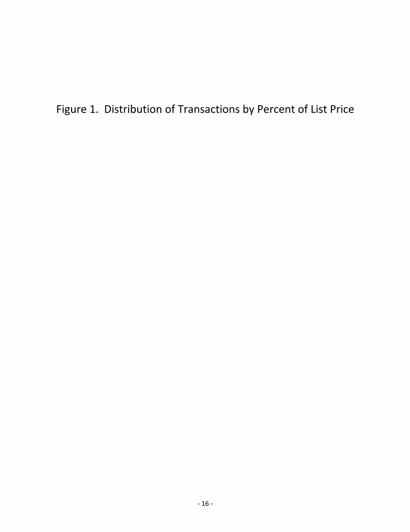
The distribution of prices as a percent of list price is represented in Figure 1. For example, just over 10

percent of transactions took place at prices between 30 and 40 percent of the retail price. Of these,

slightly under half were clearance transactions. Most notable is the absence of small discounts. Very

few purchases reduce prices to 90 percent or 80 percent of list. Instead, typical sale prices are between

30 percent and 50 percent below list price. Clearance discounts are larger still, with a mode between 70

and 80 percent off list price. Overall, the median discount is almost exactly 50 percent of list price. While

firms may change prices by changing the depth of the sale, this chain clearly does not change the

frequency of sales to change prices.

The seasonal aspect of these sales may be seen in Figure 2.

Figure 3 displays the monthly pattern of prices, sales, and transactions for one of the most common

IDNs, a particular type of short‐sleeved tee shirt. That item was sold in 16 stores, beginning in February

2006, in a total of 11,251 transactions. The list price for this IDN was $20, but the figure shows that the

average monthly transaction price was just under $15 ($14.84) in the first month and then declined

almost monotonically to under $3 ($2.82) in March 2007. A particularly sharp drop in average price,

from $10.41 to $6.93, occurred in August 2006, accompanied by a more than doubling of transactions

between July and August. The figure also shows that there were a negligible number of clearance

transactions until November 2006, after which essentially all transactions were at clearance prices.

After March 2007 the average price drifts upward, but on a base of almost no transactions (31 over the

last seven months of our sample period).

In this paper we do not explore the issue of store coupons. These coupons may be applied to any item

or set of items. While the data indicate whether or not a coupon was used, the exact nature of the

coupon must be inferred. Further, it is unclear how to estimate a cost of living index when the consumer

‐ 5 ‐

has some control over price, and when he or she benefits from a discount that may be applied to any

one of a variety of items.

C Weekday and weekend prices

Prices are collected for the U.S. Consumer Price Index (CPI) throughout the month, but almost

exclusively during weekdays. This occurs in part because managers often are too busy during the

weekend to talk to field agents sent out by the BLS. As noted above, this has the potential to bias price

indexes for apparel.

The potential becomes apparent in Figure 4. Approximately 43 percent of our misses’ tops transactions

take place on Saturday and Sunday, and nearly 60 percent of transactions occur on Friday through

Sunday. In contrast, only 1.5 percent of all quotes collected for the CPI are on Saturday and Sunday, and

only 14 percent are collected on Friday through Sunday. Average prices tend to be slightly lower on the

weekend as well. The figure shows that Friday and Saturday have the lowest average price, $13.35, and

the lowest average percent of retail price, 48 percent. That does not necessarily indicate a problem,

however. As long as prices are changing at the same rate on both weekends and weekdays, price

indexes constructed from weekday quotes should not be biased.

To examine this, in Figure 5 we plot over time simple indexes of the average price on weekdays and the

average price on weekends, with both average prices set equal to 100 in January 2004. The two indexes

do not entirely coincide: differences occur in several different periods, including the end of 2004, the

middle of 2005 and the middle of 2006. Nevertheless, the two indexes are remarkably close. This

provides evidence that relying on prices during the weekday does not bias price indexes.

D Price Trends

By reputation, the prices of apparel items are highest when they enter and lowest when they exit.3

Considerable research has been conducted on methods for comparing the price of an item when it exits

to the price of a replacement item. If no account is made of the difference – if price changes for the new

item without accounting for difference between the old and new item – CPIs will have a downward bias.

Here we describe two types of long run indexes, those formed by chaining short run indexes and those

formed by using average prices in each time period.

Figure 6 provides a histogram of the long run price trends for the IDNs in our sample. The horizontal axis

represents the average percent decline in prices per month. While there are some items that have an

upward trend, it is clear that on average the price trend is negative. The distribution has a mode of

about ‐3 percent and a median of about ‐6 percent. Figure 7 plots the month‐to‐month change in price,

calculated by comparing only prices of IDNs that appear in both months. With the exception of June,

2006, these prices of “matched models” declined significantly in every single month. Some months, such

as August 2004, show particularly sharp price declines of 20 percent or more.

3 See, for example, Guédès (2007).

‐ 6 ‐

For figures 8 and 9, we randomly select 120 IDNs and plot the paths of their average prices. Figure 8

arranges the paths from first month, whenever it occurred, through the 20th month. It shows a sharp

downward trend in the initial months. While some prices remain unchanged in the second month, many

prices have fallen, with concentrations at 80 percent and 60 percent of initial prices. After four months

many of the IDNs disappear, either temporarily or permanently. After six months, the prices of many of

the remaining IDNs have hit a minimum, and rise in the following month. The prices of many other items

continue to fall, however. By the eighth month the prices of most of the remaining goods are less than

40 percent of the prices in the first month. At the twelfth month, many items disappear. Figure 9 plots

the same paths, but starts each path at the appropriate date so that the seasonal nature of the price

paths becomes clear.

Figures 6 through 10 thus confirm our expectation that misses’ tops, like other items of apparel, trend

downward in price over time. They also highlight a fundamental problem in constructing price indexes

for apparel. Statistical agencies typically construct price indexes by selecting a sample of items and

comparing prices of identical items from month to month. As noted above, however, the median

monthly matched‐model price change in our sample is a negative 6 percent. This is demonstrated in

Figure 10, which displays the month‐to‐month index relatives in chained Laspeyres and Paasche indexes.

The monthly relatives are almost always less than one. Compounded over 45 months, this would yield

implausible drops in price indexes for misses’ tops during our study period. Evidently, construction of

an accurate price index requires some alternative to the usual matched‐model method.

Figure 11 displays the results of various alternative approaches to solving this problem. The first two are

matched‐model indexes using prices and transactions aggregated to the IDN level. One of these uses a

Chained Laspeyres formula with each IDN’s average price change weighted by the IDN’s share of

transaction value in the previous month, while the other employs a Chained Törnqvist formula based on

both the current‐month and previous‐month shares of transaction value. The difference in formula has

little effect. Both these indexes fall by more than 80 percent in the first year and end at an index value

of less than 1 on a base of 100. Recent work by Nakamura, Nakamura and Nakamura (2010) focuses on

the problem of chain drift when using transaction level data to construct indexes. That drift can occur if

prices oscillate as they move on and off sale. In the data in this paper, the relentless downward march of

prices completely overwhelm the chain drift issue.

The remaining three indexes in Figure 11 are derived from regressions on the whole set of transaction

microdata. Each regression has a set of 47 dummy variables corresponding to months after January

2004. The dependent variable in each case is the logarithm of price. The top line in the figure is the

index from a regression with only the time dummies as explanatory variables. Constructed in this way,

the index is just a measure of the geometric‐mean transaction price in each period. That index displays

fairly consistent seasonal patterns, such as troughs in February and peaks in March, but remains roughly

level in the long run. For example, the index falls by 8.9 percent between August 2004 and August 2007,

or about 2.8 percent per year.

The average‐price index behaves in a much more reasonable manner than the chained matched‐model

indexes, but has the potentially critical flaw that it fails to account for any changes in average item

‐ 7 ‐

characteristics or “quality” over time. (The BLS does not publish a CPI for this category. In the CPI

publication scheme, the lowest‐level index that includes misses’ tops is Women’s Suits and Separates.)

One way to hold quality constant is to include the item identifiers as explanatory regression variables.

When we add a dummy variable for each IDN to the regression, however, the resulting index exhibits a

decline almost as steep as those of the matched‐model indexes. In effect, including the IDN dummies

means that the effect of time will be estimated from changes in price within IDNs. That index’s final

level in October 2007 is 3.0.

It might be expected that the downward drift would be mitigated by adding to the month and IDN

dummies one more dummy variable to indicate clearance sale transaction. In that regression, the lower

prices for clearance transactions is attributed to the fact of the clearance sale rather than to the passage

of time. Figure 11 shows that the clearance dummy does, in fact, mitigate the trend, but it does not

nearly eliminate it. The associated index still falls by about 43 percent in the first year and to a level of

17.0 at the end of the 46‐month period.

E Alternative Indexes

In the previous section we showed that the standard index formulas yield implausible results, due to the

characteristic features of apparel pricing. The scanner data we use here exhibit the familiar pattern that

the BLS and other statistical agencies have observed in CPI apparel data, namely a steep and persistent

decline in price over time for any given item. Under these circumstances, any matched‐model index will

follow the same continuous decline.

Recent papers by Kevin Fox, Lorraine Ivancic, and Erwin Diewert (2009) and by Jan de Haan and

Heymerik van der Grient (2009) have demonstrated that an RGEKS (Rolling Gini‐Eltetö‐Köves‐Szulc)

index can have value in mitigating chain drift in high‐frequency scanner data such as we analyze here.

Chain drift can occur even in superlative indexes when the mix of items sold varies widely from period to

period, reducing the usable samples of price changes for individual matched items. The RGEKS model

adapts an approach used in multi‐lateral indexes by treating data for consecutive time periods as if they

were data for countries or areas. This permits the comparison of prices for like items in non‐consecutive

periods.

We computed unit‐value prices for each store‐IDN‐month combination, and constructed a 13‐month

RGEKS index based on the Törnqvist formula. Let Trs be the Törnqvist index in period r relative to period

s, formed from the unit‐value price ratios and revenue shares of the store‐IDN combinations observed in

both periods. Then for the first 13 periods of our data set the RGEKS index between periods t and t‐1 is

given by

, , ,⁄/

1, … , 13

For periods 14 and later, we compute recursively

‐ 8 ‐

, ,⁄/

Unfortunately, in our scanner data the problems associated with the apparel product life cycle equal or

outweigh the problems arising from product‐mix volatility. As a consequence, the RGEKS approach fails

to yield plausible index movements. This is demonstrated in Figure 12. The index declines in the great

majority of months, ending in October 2007 at a level of 10.5 on a base of January 2004=100.

The fundamental limitation appears to be that we cannot match prices of an identical item (IDN) over a

sufficiently long period. The shelf life of a specific IDN is almost always less than a year, and if two IDNs

are essentially identical we do not observe that fact. Therefore, we have no way to treat them as the

same item in a matched‐model index. If IDNs remained in the sample for more than a year, the cyclical

movements in their prices might be picked up by the RGEKS technique, but with life cycles of only a few

months there is no way for the RGEKS index to reflect an item’s price increase when it returns at the

beginning of a new season. This contrasts with the usual situation in the CPI, where an analyst can

sometimes follow an apparel item for more than a year (even if that item appears in more than one IDN)

or, if necessary, make a judgment about the degree of comparability between a disappearing item and

its replacement.

We therefore turned to hedonic regression as a means of dealing with the poor performance of our

matched‐model indexes. Hedonic models have been used for many years in the US CPI; see, for

example, the recent article by Craig Brown and Anya Stockburger (2006).

Our scanner data are not ideal for hedonic regression work. Table 1 lists some IDN‐level fields that

contain potentially useful product characteristics, such as Brand and Type of fabric. The most valuable is

the IDN description text field, which contains a variety of information. Unfortunately, all these fields are

blank in a large fraction of cases. Moreover, the IDN description field is not in a fixed format, and the

same characteristic can be described in multiple ways. Our descriptive variables had to be defined by

searches for specified text strings; more importantly, the absence of information on a given

characteristic is difficult to interpret. The lack of any reference to sleeve length, for example, could be

interpreted as indicating a default length or simply that the sleeve length was not coded for that item.

Despite these missing‐value problems, we proceeded to construct a large number of dummy variables

for use in hedonic regressions. The categorical information we employed is shown in table 2, along with

frequency distributions by numbers of transactions. We defined dummy variables corresponding to

each category of the variables in table 2.

Our first hedonic index was derived from a single regression using our entire data set. The explanatory

variables included the dummy variables from table 2 and for brand; dummy variables for each store in

our sample, and dummy variables for each month from February 2004 through October 2007. The

dependent variable was the logarithm of price, and the regression sample comprised 951,108

observations. The results strongly support a relationship between price and the descriptive variables we

constructed. The regression R2 was .29, and the F statistics for the significance of each explanatory

‐ 9 ‐

variable set – month, brand, sleeve length, item type, fabric, pattern, fashion, and store – were all above

100 and significant at more than the 0.0001 level. The parameter estimates and standard errors are

shown in table 3.4

Figure 13 compares the regression index results from table 3 with the average price series shown in

figure 10. The two indexes are roughly similar in their movements, and neither exhibits a clear long‐

term trend, in sharp contrast to our matched‐model indexes. Notice, however, that the regression index

ends the period at almost the same level as in January 2004, while the average price rises by

approximately 15 percent. To avoid seasonality differences, we can compare their levels in January

2007, three years after the start of the sample period. Again, in that month the regression index is

noticeably lower, by about 8 percentage points. These are relatively small differences when compared

to the volatile month‐to‐month movements of both series, but in absolute terms differences of this

magnitude after 3‐4 years is not trivial.

To explore this question, we examined the explanatory variables to identify those that account for the

apparent quality improvement over the sample period. Again to avoid intra‐year variation we compared

the months of January 2004 and January 2007. Over this time period the largest impacts of quality

change were in the item type and fabric categories. As seen in table 3 the coefficient on Tank Top is

‐0.407, indicating that, all else held constant, tank tops sold for about 33 percent less than tops for

which no type was coded. Between January 2004 and January 2007 the share of tank tops in our sample

fell from about 14 percent to about 0.4 percent, indicating an improvement in “quality” of

approximately exp[(‐.4070)*(‐.136)]‐1, or 5.7 percent. The share of tops with satin fabric also declined

between the two periods, from about 17 percent to zero, and this yielded a measured quality

improvement of approximately 4.2 percent. Computing and aggregating the same effects for all the

other regressor variables explains the cumulative difference of about eight percentage points between

the indexes in figure 13.

Although our regression results and the associated quality trends are plausible, we recognize that they

may be an artifact of our data. It is possible that the changes in sample shares for tank tops, satin fabric,

and other item characteristics could merely reflect changes in coding procedures. As noted above, the

categories of explanatory variables were not defined by the retailer; we defined them based on the

types of information shown in the IDN description text field. Between 2004 and 2007 the share of

purchases with coded values of fabric and pattern fell, while the corresponding shares for sleeve length,

item type, and fashion rose. It is certainly possible that trends in our measured quality variables do not

accurately reflect trends in the actual sample characteristics. Nevertheless, taking our table 3 regression

results as a guide, we proceed to examine whether operational hedonic regression methods could yield

similar index results.

We took two approaches to computing hedonic indexes for misses’ tops using only data available during

the month for which the index value applies. First, we constructed an index from a series of 45 month‐

to‐month regressions. Each regression employed two calendar months of individual purchase data and

4 The brand and store coefficients are not shown, so as to preserve confidentiality.

‐ 10 ‐

contained all of our quality dummy variables for store, brand, and the characteristics in table 2, plus a

time dummy for the second month of the two‐month period. The time dummy coefficients from these

45 overlapping monthly regressions were then exponentiated and chained to produce an index series

for our sample period.

The second approach was based on rolling 13‐month regressions, in the spirit of the rolling RGEKS

indexes discussed above. We again estimated overlapping regressions with the same sets of

explanatory variables, but each of these 34 regressions contained 13 months of data and 12 time

dummy variables for months. The first regression covered January 2004 through January 2005, and our

index for those months was derived by exponentiating and chaining the 12 time dummy coefficients.

Then, we computed the index change in February 2005 based on the dummy for that month in our

second regression, which contained data for the 13 months from February 2004 through February 2005.

That procedure was then followed for the remaining 32 months, ending with a regression with data for

October 2006 through October 2007.

These approaches would give the same index results as that from the full table 3 regression if the

coefficients on the item characteristic variables were stable from period to period. On the other hand,

the chained month‐to‐month and rolling 13‐month methods could break down if the coefficient vectors

are volatile. In particular, the risk is that whenever new items are introduced at a high initial price, the

regression will identify the characteristics of those items as carrying high “quality” premiums. That is,

with so many explanatory variables the differences in relative prices for incoming apparel items may all

be attributed by the regression to quality differences, with the time dummy coefficient merely reflecting

the downward trends in prices of continuing items.

This disappointing result is reflected in the three hedonic indexes displayed in figure 14. The index

based on the month‐to‐month regressions is roughly similar to the matched‐model indexes in figure 10,

declining from 100 in January 2004 to 4.5 in October 2007. The rolling 13‐month regressions produce a

much more reasonable pattern, but it is still clearly downward‐biased relative to the full regression

index from figure 13. The monthly index changes for each of these three indexes are shown in figure 15.

That figure demonstrates that each index reflecting the same monthly fluctuations in price change, but

the monthly index changes are consistently highest in the full regression index and lowest in the month‐

to‐month regression index.

The largest difference between the estimates of monthly price change between the full and rolling 13‐

month regression indexes comes in February 2005, where the two models yield about 19 percent and 5

percent index increases, respectively. Again, we can highlight some of the individual regression

coefficients to explain this difference. February 2005 was a month in which there was an influx of short‐

sleeve shirts, with the sample share rising to about 16 percent from about two percent in January. The

full regression has a coefficient of ‐0.108 on short‐sleeve shirts, as seen in table 3, so ceteris paribus the

increased sample share is treated as a quality decrease. By contrast, the rolling 13‐month regression for

February 2004 through February 2005 has a coefficient of 0.474 on short‐sleeve shirts, implying that

they have very high relative quality. This coefficient difference by itself accounts for about 40 percent of

the total difference in index change estimated by the two models in February 2005. This is an

‐ 11 ‐

illustration of the effect described in the previous paragraph, where coefficient volatility in the chained

regressions can mask the price increases that occur when new items enter the sample. We note that in

the rolling 13‐month regressions the coefficient on short‐sleeve shirts declined throughout the spring

and summer and was ‐0.026 in the regression for September 2004 through September 2005.

Our general conclusion from the results of this section is that only the hedonic regression produces

indexes that are free of significant downward drift. Moreover, only the full‐period hedonic index based

on a regression using all 46 months of data yields a plausible index. None of our alternative monthly

indexes is clearly superior to the simple index of weighted‐average log‐prices.

Conclusion

In many ways the data we employ in this paper provide the ideal basis for a consumer price index. The

data set contains almost one million observations over a period of 46 months on prices for misses’ tops.

We can observe individual transaction prices along with a store identifier, the list price, and, in a large

proportion of cases, detailed item characteristics. The great variety of discounts used in apparel pricing

are fully reflected here.

Moreover, the data clearly demonstrate the dominant facts of the apparel industry: the size and

prevalence of discounts from list price, the timing and importance of clearance sales, the large share of

weekend purchases, the significant rate of product turnover, and the consistent downward trend of

prices within a given item’s lifecycle. The data also are rich enough to enable us to reject the

hypothesis, at least for this product category, that weekday price collection causes a bias in the CPI.

Against these advantages stand the well‐known difficulties of developing price indexes for apparel,

particularly a fashion item like misses’ tops. We computed monthly chained matched‐model indexes by

applying the traditional Laspeyres and superlative Törnqvist formulas to our data. Both formulas yielded

implausible indexes that fell by more than 99 percent over our sample period. Concluding that the

problem arose from the high month‐to‐month turnover in the mix of items sold, we constructed an

index using a 13‐month Rolling GEKS approach, but that index exhibited almost as great a decline as the

monthly‐chained indexes. We then turned to regression‐based indexes using dummy variables to reflect

detailed item characteristics such as brand and fabric. Due to coefficient instability over time, however,

both monthly‐chained and 13‐month rolling regression indexes declined persistently and implausibly

over our sample period.

The operational consumer price indexes for apparel indexes published by national statistical agencies

rely on careful matching of identical items, usually combined with special procedures to deal with short

product life spans. The BLS, for example, uses hedonic regressions to facilitate comparisons of the

prices of exiting and entering items. None of the approaches we tested in this paper demonstrated any

superiority to those statistical agency procedures, despite our large and detailed data set.

Nevertheless, we plan to continue to search for ways to fulfill the promise of these scanner data by

obtaining reliable, quality adjusted indexes for apparel.

‐ 12 ‐

Table 1. Variables on Data FileID Number Outlet ID Date of transaction Earliest date the product is available The planned date for the IDN to be out of stock Coupon used Type of Coupon Brand Type of fabric Item type/style IDN description (typically style and brand info) Size of item sold Size range of IDN Number of days the item was available Price paid by customer Amount of employee discount Type of discount Amount of discount List price

‐ 13 ‐

Table 2. Examples of Item Characteristics Sleeve Type Frequency Percent

Sleeveless 51,966 5.4

Cap 36,780 3.8

Short sleeve 158,214 16.3

Rouche 28,690 3.0

Flutter 8,752 0.9

Ruffle 28,853 3.0

Puff 6,690 0.7

Volume 1,763 0.2

Pleated 2,582 0.3

Elbow 3,609 0.4

Lantern 2,794 0.3

3/4 length 149,419 15.4

Long sleeve 191,093 19.7

Other or Unknown 297,279 30.7

Total 968,484 100.0

Item Type Frequency Percent

Blouse 120,210 12.4

Pullover 15,722 1.6

Tank top 18,333 1.9

Camisole 146,259 15.1

Shell 24,881 2.6

Jersey 3,166 0.3

Tunic 20,858 2.2

Dress shirt 1,154 0.1

Turtleneck 3,753 0.4

Tee 114,670 11.8

Baby Doll 3,425 0.4

Knit shirt 19 ‐

Wrap shirt 30,669 3.2

Stretch shirt 31,562 3.3

Classic 8,825 0.9


Total 968,484 100.0

‐ 14 ‐

Table 2. ContinuedFabric Frequency Percent

Silk 14,558 1.5

Satin 7,188 0.7

Lace 98,124 10.1

Mesh 22,708 2.3


Total 968,484 100.0

Pattern Frequency Percent

Solid 65,571 6.8

Print or Pattern 46,304 4.8


Total 968,484 100.0

Miscellaneous Frequency Percent

Basic 104,269 10.8

Fashion 83,182 8.6

Easy Care 71,914 7.4


Total 968,484 100.0

‐ 15 ‐

Table 3. Full Period Regression Coefficients

Variable Coefficient Standard Error t‐statistic

Sleeveless ‐0.0805 0.0025 ‐32.8

Cap ‐0.0774 0.0028 ‐28.0

Short sleeve ‐0.1080 0.0018 ‐61.3

Rouche 0.1454 0.0030 49.0

Flutter ‐0.0478 0.0056 ‐8.5

Ruffle ‐0.0269 0.0033 ‐8.2

Puff 0.0951 0.0058 16.4

Volume 0.2850 0.0109 26.1

Pleated 0.1676 0.0162 10.4

Elbow 0.2647 0.0076 34.7

Lantern 0.2744 0.0089 30.8

3/4 length 0.0162 0.0019 8.7

Long sleeve 0.1469 0.0018 82.2

Blouse 0.0349 0.0019 18.6

Pullover 0.0715 0.0040 18.0

Tank top ‐0.4073 0.0039 ‐105.8

Camisole ‐0.1977 0.0021 ‐96.1

Shell ‐0.1289 0.0034 ‐38.4

Jersey 0.1233 0.0109 11.3

Tunic 0.0631 0.0036 17.4

Dress shirt 0.1455 0.0208 7.0

Turtleneck 0.2100 0.0084 25.1

Tee ‐0.1771 0.0021 ‐85.2

Baby Doll 0.1086 0.0078 13.9

Knit shirt 0.4094 0.1044 3.9

Wrap shirt 0.1166 0.0028 41.0

Stretch shirt 0.0714 0.0029 24.8

Classic ‐0.0744 0.0051 ‐14.5

Silk 0.0100 0.0040 2.5

Satin ‐0.2342 0.0056 ‐41.7

Lace 0.0099 0.0019 5.3

Mesh 0.0545 0.0033 16.7

Solid 0.0303 0.0020 15.0

Print or Pattern ‐0.0010 0.0024 ‐0.4

Basic ‐0.2196 0.0020 ‐109.1

Fashion ‐0.2804 0.0021 ‐135.4

Easy Care ‐0.0057 0.0022 ‐2.6

‐ 16 ‐

Figure 1. Distribution of Transactions by Percent of List Price

‐ 17 ‐

Figure 2: Mean Price as a percent of List price

30%

35%

40%

45%

50%

55%

60%

65%

Mar Apr May Jun Jul Aug Sep Oct Nov Dec Jan Feb

2004/2005 2005/2006 2006/2007 2007

‐ 18 ‐

Figure 3. Monthly Transactions and Average Prices S/S Tee Shirt Item

0

200

400

600

800

1000

1200

1400

0

2

4

6

8

10

12

14

16

Number of Transactions

Price

Year and Month

Total Transactions Clearance Transactions Average Price

‐ 19 ‐

Figure 4. Transactions and Prices by Day of Week

‐ 20 ‐

Figure 5. Indexes of Average Prices (200401=1)

‐ 21 ‐

Figure 6. Average Monthly Rates of Price Change

‐ 22 ‐

Figure 7. Monthly Matched‐Model Rates of Price Change

‐ 23 ‐

Figure 8. Indexes of Average Price, 120 IDNs, First 20 Months

‐ 24 ‐

Figure 9. Indexes of Average Price, 120 IDNs, by Sample Month

0

20

40

60

80

100

120

140

160

180

200

200401

200402

200403

200404

200405

200406

200407

200408

200409

200410

200411

200412

200501

200502

200503

200504

200505

200506

200507

200508

200509

200510

200511

200512

200601

200602

200603

200604

200605

200606

200607

200608

200609

200610

200611

200612

200701

200702

200703

200704

200705

200706

200707

200708

200709

200710

‐ 25 ‐

Figure 10. Laspeyres and Paasche Month‐Month Indexes

0.6

0.65

0.7

0.75

0.8

0.85

0.9

0.95

1

1.05

Laspeyres Paasche

‐ 26 ‐

Figure 11. Alternative Price Indexes for Misses’

Tops (200401 = 1)

0

0.2

0.4

0.6

0.8

1

1.2

1.4

1.6

Chained Tornqvist Chained LaspeyresAverage Log Price Time Dummies + IDNsTime Dummies + IDNs + Clearance

‐ 27 ‐

Figure 12. Rolling 13‐month GEKS Index (January 2004=100)

0

20

40

60

80

100

120

Month

‐ 28 ‐

Figure 13. Average Log Price and Full Regression Index (January 2004=100)

0

20

40

60

80

100

120

140

160

Average Log Price Full Hedonic Regression

‐ 29 ‐

Figure 14. Full Regression Index, Monthly Chained Index, and Rolling 13‐month Chained Index, January 2004=100

0

20

40

60

80

100

120

140

160

Full Regression Monthly Chained Rolling 13‐Month

‐ 30 ‐

Figure 15. Month‐to‐month Log Changes, Full Regression Index, Monthly Chained Index, and Rolling 13‐month Chained Index

‐0.6

‐0.4

‐0.2

0

0.2

0.4

0.6

0.8

1

1.2

‐ 31 ‐

References

Bils, Mark (1989): "Pricing in a Customer Market," Quarterly Journal of Economics, pp. 699‐718,

November.

Bils, Mark, and Peter Klenow (2004): “Some evidence on the importance of sticky prices,” Journal of

Political Economy, v. 112, pp. 947‐985, October.

Brown, Craig, and Anya Stockburger (2006): “Item replacement and quality change in apparel price

indexes,” Monthly Labor Review, v. 129, pp. 35‐45, December. Available at

http://www.bls.gov/opub/mlr/2006/12/art3full.pdf.

Chevalier, Judith A., and Anil K. Kashyap (2010): “Best Prices,” manuscript, July.

Chevalier, Judith A., Anil K. Kashyap, and Peter E. Rossi (2003), "Why Don't Prices Rise During Periods of

Peak Demand? Evidence from Scanner Data," American Economic Review, v. 93, pp. 15‐37, March.

de Haan, Jan, and Heymerik van der Grient (2009): “Eliminating Chain Drift in Price Indexes Based on

Scanner Data,” presented at the Eleventh Meeting of the Ottawa Group, Neuchatel, Switzerland, April.

Available at

http://www.ottawagroup.org/Ottawa/ottawagroup.nsf/51c9a3d36edfd0dfca256acb00118404/c0b785f

3c0f0f765ca25727300107fd9?OpenDocument.

Eichenbaum, Martin, Nir Jaimovich, and Sergio Rebelo (2008): “Reference Prices and Nominal

Rigidities,” NBER Working Paper 13829, March.

Fox, Kevin, Lorraine Ivancic, and W. Erwin Diewert (2009): “Scanner Data, Time Aggregation and the

Construction of Price Indexes,” presented at the Annual Meeting of the American Economic Association,

January 4. Forthcoming, Journal of Econometrics. Available at

http://www.aeaweb.org/assa/2009/index.php.

Guédès, Dominique (2007) “Fashion and Consumer Price Index,” presented at the Tenth Meeting of the

Ottawa Group, Ottawa, Canada, October. Available at

http://www.ottawagroup.org/Ottawa/ottawagroup.nsf/51c9a3d36edfd0dfca256acb00118404/c0b785f

3c0f0f765ca25727300107fd9?OpenDocument.

Kashyap, Anil (1995): “Sticky Prices: New Evidence from Retail Catalogs,” Quarterly Journal of

Economics, v. 110, pp. 245‐74, February.

Lazear, Edward P. (1986): “Retail Pricing and Clearance Sales,” American Economic Review, v. 76, pp. 14‐

32, March.

Nakamura, Alice, Emi Nakamura, and Leonard I. Nakamura (2010): “Price Dynamics, Retail Chains and

Inflation Measurement,” manuscript, March.

‐ 32 ‐

Pashigian, B. Peter, and Brian Bowen (1991): “Why are Products Sold on Sale?: Explanations of Pricing

Regularities,” Quarterly Journal of Economics, pp. 1015‐1038, November.

superlative and regression based consumer price indexes ... · pdf filesuperlative and...

Documents