supermassive black hole binaries and transient radio events
TRANSCRIPT
Supermassive Black Hole Binaries
and Transient Radio Events:
Studies in Pulsar Astronomy
Sarah Burke Spolaor
Presented in fulfillment of the requirements
of the degree of Doctor of Philosophy
2011
Faculty of Information and Communication Technology
Swinburne University

i
Abstract
The field of pulsar astronomy encompasses a rich breadth of astrophysical topics.
The research in this thesis contributes to two particular subjects of pulsar astronomy:
gravitational wave science, and identifying celestial sources of pulsed radio emission.
We first investigated the detection of supermassive black hole (SMBH) binaries, which
are the brightest expected source of gravitational waves for pulsar timing. We consid-
ered whether two electromagnetic SMBH tracers, velocity-resolved emission lines in active
nuclei, and radio galactic nuclei with spatially-resolved, flat-spectrum cores, can reveal
systems emitting gravitational waves in the pulsar timing band. We found that there are
systems which may in principle be simultaneously detectable by both an electromagnetic
signature and gravitational emission, however the probability of actually identifying such
a system is low (they will represent ≪1% of a randomly selected galactic nucleus sample).
This study accents the fact that electromagnetic indicators may be used to explore binary
populations down to the “stalling radii” at which binary inspiral evolution may stall indef-
initely at radii exceeding those which produce gravitational radiation in the pulsar timing
band. We then performed a search for binary SMBH holes in archival Very Long Base-
line Interferometry data for 3114 radio-luminous active galactic nuclei. One source was
detected as a double nucleus. This result is interpreted in terms of post-merger timescales
for SMBH centralisation, implications for “stalling”, and the relationship of radio activity
in nuclei to mergers. Our analysis suggested that binary pair evolution of SMBHs (both
of masses >108 M⊙) spends less than 500Myr in progression from the merging of galactic
stellar cores to within the purported stalling radius for SMBH pairs, giving no evidence for
an excess of stalled binary systems at small separations. Circumstantial evidence showed
that the relative state of radio emission between paired SMBHs is correlated within orbital
separations of 2.5 kpc.
We then searched for transient radio events in two archival pulsar surveys, and in
the new High Time Resolution Universe (HTRU) Survey. We present the methodology
employed for these searches, noting the novel addition of methods for single-event recog-
nition, automatic interference mitigation, and data inspection. 27 new neutron stars were
discovered. We discuss the relationship between “rotating radio transient” (RRAT) and
pulsar populations, finding that the Galactic z-distribution of RRATs closely resembles
the distribution of pulsars, and where measurable, RRAT pulse widths are similar to in-
dividual pulses from pulsars of similar period, implying a similar beaming fraction. We
postulate that many RRATs may simply represent a tail of extreme-nulling pulsars that
are “on” for less than a pulse period; this is supported by the fact that nulling pulsars and
single-pulse discoveries exhibit a continuous distribution across null/activity timescales
and nulling fractions. We found a drop-off in objects with emissivity cycles longer than
ii
∼300 seconds at intermediate and low nulling fractions which is not readily explained by
selection effects. The HTRU deep low-latitude survey (70-min. pointings at galactic lati-
tudes |b| < 3.5 and longitudes −80 < l < 30) will be capable of exploring whether this
deficit is natural or an effect of selection. The intriguing object PSR J0941–39 may rep-
resent an evolutionary link between nulling populations; discovered as an sparsely-pulsing
RRAT, in follow-up observations it often appeared as a bright (10 mJy) pulsar with a low
nulling fraction. It is therefore apparent that a neutron star can oscillate between nulling
levels, much like mode-changing pulsars. Crucially, the RRAT and pulsar-mode emission
sites are coincident, implying that the two emission mechanisms are linked. We estimate
that the full HTRU survey will roughly quadruple the known deep-nulling pulsar popu-
lation, allowing statistical studies to be made of extreme-nulling populations. HTRU’s
low-latitude survey will explore the neutron star population with null lengths lasting up
to several hours.
We lastly reported the discovery of 16 pulses, the bulk of which exhibit a frequency
sweep with a shape and magnitude resembling the “Lorimer Burst” (Lorimer et al. 2007),
which three years ago was reported as a solitary radio burst that was thought to be the
first discovery of a rare, impulsive event of unknown extragalactic origin. However, the
new events were of clearly terrestrial origin, with properties unlike any known sources of
terrestrial broad-band radio emission. The new detections cast doubt on the extragalactic
interpretation of the original burst, and call for further sophistication in radio-pulse sur-
vey techniques to identify the origin of the anomalous terrestrial signals and definitively
distinguish future extragalactic pulse detections from local signals. The ambiguous origin
of these seemingly dispersed, swept-frequency signals suggest that radio-pulse searches us-
ing multiple detectors will be the only experiments able to provide definitive information
about the origin of new swept-frequency radio burst detections.
Finally, we summarise our major findings and suggest future work which would expand
on the work in this thesis.
iii
AcknowledgementsMany good people have contributed to the completion of this thesis and to the unique
period of personal and professional growth that the past few years have represented.
I owe a big round of thanks to four great supervisors, Matthew Bailes, Dick Manchester,
Simon Johnston, and David Barnes, who each in their way has constantly conveyed an
excitement for science and the scientific process that I strive to replicate. I appreciate
the scientific and personal support offered by all of them at various times, as well as
the space and encouragement they gave to explore my own ideas (and patient support
through those “bold claims,” as Matthew would say, that came from left-field ideas!).
All of these elements were essential in navigating successfully through this period, and
my closer supervisors, Dick, Simon, and Matthew, all made crucial contributions to my
education and to developing the scientific ideas explored by this thesis. I would like to
particularly thank my primary supervisor, Matthew, for being an important role model
for balancing the importance of family with a strong astronomical career. I have a great
respect for the leadership he has shown over the course of my PhD.
I am tremendously grateful to have had the chance to interact closely with both Ron
Ekers and George Hobbs. Ron first introduced me to the Australian scientific community
and has always been a valuable sounding board for new ideas, a like-minded brainstorm
companion, a constant source of encouragement and way-out-of-the-box thinking, a men-
tor, and a good friend. George has likewise been an indespensable part of my candidature,
often providing a house filled with good music, food, films, and strange board games, and
always providing insightful discussions on pulsar and extragalactic astronomy. I must ex-
press appreciation for those who laid the seeds of my scientific career early on through
dedicated and creative teaching. This includes Doc Stoneback, Steve Boughn, Walter
Smith, and the person who first introduced me to the world of scientific research and to
the Universe through cosmology, Prof. Bruce Partridge.
A very general thanks go to the staff and scientists at Swinburne Ctr. for Astrophysics,
ATNF Marsfield, and Parkes Telescope: rest assured all of you helped make each of these
places welcoming, engaging institutions. I hold special thanks for a few: the post-docs
at Swinburne who let me wander into their offices to either chat idly, snatch books off
their shelves, nag them about code bugs, or deliberate about a range of topics—Willem,
Ramesh, Andrew, and Jonathon, thanks for all that. It has been a pleasure to learn from
such knowledgeable scientists, and in many cases, have sources of light relief in S. Amy,
B. Koribalski, J. Reynolds, G. Carrad, T. Tzioumis, R. Hollow, C. Cliff, J. Caswell,
T. Cornwell, R. Smits, R. Jenet, Shirley and Janette, J. Khoo, DJ Champion, E. Sadler,
A. Graham, T. Murphy, M. Kesteven, M. Keith, P. Weltevrede, and D. Schnitzeler. Big
thanks are owed to John Sarkissian for the countless late-night chats about everything in

iv
the world, and the tireless help with observing.
My fellow students and friends have been necessary stress relievers along the way,
particularly my “not-really-band-mates” Joris, Carlos, Chris, and Max, as well as many
others in and out of work like Lina, Stefan, Evelyn, Adam, Juan, Adrian, Francesco,
Caterina, Andy, Ben, Amanda and Jonathon, Marc, Glenn, Nigel, Nick Jones, Minnie,
Katherine Newton-McGee, Peter and Sofie. I hope to see you all again many times in the
coming years of our careers.
Last and anything but least, I acknowledge the invaluable and ongoing support of
my family. From my beginning, my parents have taught and encouraged me to pursue
every interest in and out of this world; they, my siblings Hannah and Ryan, JPL, and my
extended family have represented a wonderful source of many different kinds of wisdom
and friendship in my life. Which reminds me: thanks, Uncle Dean, for emailing me from
time to time to inform me how cool astronomy is! Finally, Max Spolaor is my husband
and closest friend. He gives me confidence when I feel I have none, is a constant reminder
of what is most important in this world, and has been my strongest support in and out of
work over the past three years.
Thanks everybody! Oh, and by the way Lizz and Jono, thanks for all the eBoggle!

v
vi
Declaration
The work presented in this thesis has been carried out in the Centre for Astrophysics
& Supercomputing at the Swinburne University of Technology (Hawthorn, VIC) and the
Australia Telescope National Facility/CSIRO Astronomy and Space Sciences (Marsfield,
NSW) between 2007 and 2010. This thesis contains no material that has been accepted
for the award of any other degree or diploma. To the best of my knowledge, this thesis
contains no material previously published or written by another author, except where
due reference is made in the text of the thesis. Several chapters have been partially or in
entirety published in refereed journals; these are listed below. Minor alterations have been
made to the published papers in order to maintain argument continuity and consistency
of spelling and style.
• Chapter 3 has been published by the Monthly Notices of the Royal Astronomical
Society (MNRAS) as “A Radio Census of Binary Supermassive Black Holes”, 2011,
MNRAS, v. 410, p. 2113, authored by S. Burke-Spolaor.
• Chapter 4 was published as “The Millisecond Radio Sky: Transients from a Blind
Single Pulse Search”, 2010, MNRAS, v. 402, p. 855, authored by S. Burke-Spolaor
and M. Bailes.
• Chapter 5 has been accepted to MNRAS as “The High Time Resolution Universe
Survey - II. Single-pulse Search and Early Discoveries”, authored by S. Burke-Spolaor
on behalf of the HTRU survey team: M. Bailes, S. Bates, N. D. R. Bhat, M. Burgay,
N. D’Amico, S. Johnston, L. Levin, M. Keith, M. Kramer, S. Milia, A. Possenti,
B. Stappers. and W. van Straten. It will appear in print in early 2011.
• Chapter 6 was published by the Astrophysical Journal Letters as “Radio Bursts with
Extragalactic Spectral Characteristics Show Terrestrial Origins”, 2011, v. 727, p. 18,
authored by S. Burke-Spolaor, M. Bailes, R. Ekers, J-P. Macquart, and F. Crawford.
Sarah Burke Spolaor
Melbourne, Australia
June 2011

vii
Dedicated to Grandpa Burke, Grandpa
Munson, Ethel, Dale, and Mickey.
Wish you were here!

Contents
Abstract i
Acknowledgements iii
Statement of Originality vi
List of Figures xiii
List of Tables xv
1 Introduction 1
1.1 Pulsars . . . . . . . . . . . . . . . . . . . . . . . . . . . . . . . . . . . . . . . 1
1.1.1 Pulsar Energetics and Physical Parameters . . . . . . . . . . . . . . 2
1.1.2 Basic Radio Observables and the Interstellar Medium . . . . . . . . 4
1.1.3 Pulsar Varieties . . . . . . . . . . . . . . . . . . . . . . . . . . . . . . 9
1.2 Pulsar Timing and Timing Arrays . . . . . . . . . . . . . . . . . . . . . . . 11
1.3 Gravitational Wave Astronomy . . . . . . . . . . . . . . . . . . . . . . . . . 13
1.3.1 Sources of Gravitational Radiation . . . . . . . . . . . . . . . . . . . 13
1.3.2 GW Signals and Timing Sensitivity . . . . . . . . . . . . . . . . . . 16
1.4 Pulsar Searches and Fast-Transient Radio Astronomy . . . . . . . . . . . . 17
1.4.1 Considerations in Pulsar Survey Design . . . . . . . . . . . . . . . . 17
1.4.2 Periodicity Searches and the Re-advent of Single Pulse Searching . . 18
1.4.3 Known Sources of Fast Transient Radio Emission . . . . . . . . . . . 22
1.4.4 Unknown & Theoretical Sources of Fast Transient Radio Emission . 23
1.5 Thesis Outline . . . . . . . . . . . . . . . . . . . . . . . . . . . . . . . . . . 24
2 Co-detectability of Gravitational and Electromagnetic Waves 27
2.1 Introduction . . . . . . . . . . . . . . . . . . . . . . . . . . . . . . . . . . . . 28
2.2 Electromagnetic SMBH Signatures . . . . . . . . . . . . . . . . . . . . . . . 29
2.3 Physical Preliminaries . . . . . . . . . . . . . . . . . . . . . . . . . . . . . . 31
2.4 Capabilities of Electromagnetic Detection Techniques . . . . . . . . . . . . . 32
2.4.1 Direct Imaging Techniques . . . . . . . . . . . . . . . . . . . . . . . 32
2.4.2 Spectral Line Techniques . . . . . . . . . . . . . . . . . . . . . . . . 32
2.5 Co-observable Binary Systems . . . . . . . . . . . . . . . . . . . . . . . . . . 33
2.6 Practical Considerations . . . . . . . . . . . . . . . . . . . . . . . . . . . . . 34
2.6.1 Prospects of System Co-detection . . . . . . . . . . . . . . . . . . . . 34
ix
x Contents
2.6.2 Sensitivity Considerations for Pulsar Timing . . . . . . . . . . . . . 38
2.7 Conclusions . . . . . . . . . . . . . . . . . . . . . . . . . . . . . . . . . . . . 38
3 A Search for Binary Supermassive Black Holes 41
3.1 Introduction . . . . . . . . . . . . . . . . . . . . . . . . . . . . . . . . . . . . 41
3.2 The Archival Data Sample . . . . . . . . . . . . . . . . . . . . . . . . . . . . 45
3.2.1 Notes on potential selection effects . . . . . . . . . . . . . . . . . . . 46
3.3 VLBI Search for Double AGN . . . . . . . . . . . . . . . . . . . . . . . . . . 46
3.4 Candidates and Search Results . . . . . . . . . . . . . . . . . . . . . . . . . 49
3.4.1 Candidates with Active Relativistic Injection . . . . . . . . . . . . . 51
3.5 Framework for Interpretation . . . . . . . . . . . . . . . . . . . . . . . . . . 54
3.5.1 Supermassive Black Holes and Radio Emission . . . . . . . . . . . . 56
3.5.2 Host Properties and Limiting Radii . . . . . . . . . . . . . . . . . . 58
3.5.3 Spatial Limits of the Search . . . . . . . . . . . . . . . . . . . . . . . 60
3.5.4 Galaxy Merger Rates . . . . . . . . . . . . . . . . . . . . . . . . . . 61
3.6 Limits on Inspiral Timescales for SMBH Binaries . . . . . . . . . . . . . . . 62
3.7 Discussion . . . . . . . . . . . . . . . . . . . . . . . . . . . . . . . . . . . . . 63
3.7.1 Post-merger Efficiency, Radio Ignition, and SMBH Binary Stalling . 64
3.7.2 Consequences for the GW Background and Pulsar Timing Arrays . . 65
3.8 Summary . . . . . . . . . . . . . . . . . . . . . . . . . . . . . . . . . . . . . 66
4 Transients in Archival Pulsar Surveys 67
4.1 Introduction . . . . . . . . . . . . . . . . . . . . . . . . . . . . . . . . . . . . 67
4.1.1 A Brief History of Single Pulse Searching . . . . . . . . . . . . . . . 68
4.1.2 The Ambiguous Nature of RRATs . . . . . . . . . . . . . . . . . . . 68
4.2 Data Sample . . . . . . . . . . . . . . . . . . . . . . . . . . . . . . . . . . . 69
4.3 Single Burst Search Process . . . . . . . . . . . . . . . . . . . . . . . . . . . 72
4.4 Results . . . . . . . . . . . . . . . . . . . . . . . . . . . . . . . . . . . . . . . 75
4.4.1 New Transient Sources . . . . . . . . . . . . . . . . . . . . . . . . . . 75
4.5 Discussion . . . . . . . . . . . . . . . . . . . . . . . . . . . . . . . . . . . . . 81
4.5.1 Pulsar Transient Varieties and the Nature of RRAT Emission . . . . 81
4.5.2 A Breakdown of Our Discoveries . . . . . . . . . . . . . . . . . . . . 84
4.5.3 Exploration of RRATs and the Properties of Our New Discoveries . 85
4.6 Summary . . . . . . . . . . . . . . . . . . . . . . . . . . . . . . . . . . . . . 91
Contents xi
5 Transients in the High Time Resolution Universe Survey 93
5.1 Introduction . . . . . . . . . . . . . . . . . . . . . . . . . . . . . . . . . . . . 93
5.2 The HTRU Survey’s Single-pulse (SP) Search . . . . . . . . . . . . . . . . . 95
5.2.1 Data Analysis Pipeline . . . . . . . . . . . . . . . . . . . . . . . . . . 95
5.2.2 Search Sensitivity . . . . . . . . . . . . . . . . . . . . . . . . . . . . 101
5.2.3 Current Processing Status . . . . . . . . . . . . . . . . . . . . . . . . 104
5.2.4 Candidate Ranking and Follow-up Strategy . . . . . . . . . . . . . . 106
5.3 Early Discoveries & Detections . . . . . . . . . . . . . . . . . . . . . . . . . 107
5.3.1 New Discoveries . . . . . . . . . . . . . . . . . . . . . . . . . . . . . 107
5.3.2 Redetections of Known Pulsars and RRATs . . . . . . . . . . . . . . 110
5.4 Discussion . . . . . . . . . . . . . . . . . . . . . . . . . . . . . . . . . . . . . 111
5.4.1 Our Discoveries in Archival Pulsar Surveys . . . . . . . . . . . . . . 111
5.4.2 Activity Timescales in Sparsely-emitting Neutron Stars . . . . . . . 112
5.4.3 Detectability of Intermittent Neutron Star Populations . . . . . . . . 116
5.4.4 Discovery Forecast for the Full HTRU Survey . . . . . . . . . . . . . 117
5.5 Summary and Conclusions . . . . . . . . . . . . . . . . . . . . . . . . . . . . 118
6 Anomalous, Terrestrial Lorimer-Burst Signals in Pulsar Data 121
6.1 Introduction . . . . . . . . . . . . . . . . . . . . . . . . . . . . . . . . . . . . 121
6.2 Data Set and Search . . . . . . . . . . . . . . . . . . . . . . . . . . . . . . . 122
6.3 New Discoveries and Their Properties . . . . . . . . . . . . . . . . . . . . . 124
6.3.1 Flux and Spectral Properties . . . . . . . . . . . . . . . . . . . . . . 124
6.3.2 Evidence for a Terrestrial Origin . . . . . . . . . . . . . . . . . . . . 125
6.4 Discussion . . . . . . . . . . . . . . . . . . . . . . . . . . . . . . . . . . . . . 128
6.4.1 Signal Origins . . . . . . . . . . . . . . . . . . . . . . . . . . . . . . . 128
6.4.2 Investigation of Atmospheric Plasma Emission Origins . . . . . . . . 129
6.4.3 Weather-related Effects . . . . . . . . . . . . . . . . . . . . . . . . . 132
6.5 A Closer Look at the Lorimer Burst . . . . . . . . . . . . . . . . . . . . . . 132
6.6 Conclusions . . . . . . . . . . . . . . . . . . . . . . . . . . . . . . . . . . . . 134
7 Conclusions and Future Directions 139
7.1 Conclusions and Major Findings of this Thesis . . . . . . . . . . . . . . . . 139
7.2 Future directions . . . . . . . . . . . . . . . . . . . . . . . . . . . . . . . . . 141
Bibliography 145

xii Contents
A Useful Constants and Conversions 157
List of Figures
1.1 Pulsar radio lifetime . . . . . . . . . . . . . . . . . . . . . . . . . . . . . . . 3
1.2 The P − P diagram . . . . . . . . . . . . . . . . . . . . . . . . . . . . . . . 5
1.3 Duty cycle as a function of pulse width . . . . . . . . . . . . . . . . . . . . . 6
1.4 Waterfall plot showing ISM effects for a low-DM pulsar . . . . . . . . . . . 8
1.5 The gravitational radiation spectrum . . . . . . . . . . . . . . . . . . . . . . 14
1.6 Standard Pulsar and Single Pulse Searches . . . . . . . . . . . . . . . . . . . 19
1.7 Radio Transient Phase Space . . . . . . . . . . . . . . . . . . . . . . . . . . 21
2.1 Evolution of Supermassive Binaries . . . . . . . . . . . . . . . . . . . . . . . 29
2.2 Parameter space of SMBH inspiral stages explored by VLBI . . . . . . . . . 35
2.3 Overlap of systems detectable in electromagnetic and gravitational waves . 36
2.4 Redshift distribution of radio-emitting galaxies . . . . . . . . . . . . . . . . 37
3.1 Redshift distribution of our data sample . . . . . . . . . . . . . . . . . . . . 45
3.2 Spectral index maps showing morphological categories . . . . . . . . . . . . 48
3.3 Spectral index maps showing binary candidates . . . . . . . . . . . . . . . . 50
3.4 Average minimum and maximum resolvable linear scales against redshift . . 59
3.5 Minimum resolvable linear scale for 1575 sources . . . . . . . . . . . . . . . 59
3.6 Merger and binary SMBH fraction versus redshift . . . . . . . . . . . . . . . 61
3.7 Limits on inspiral timescale in three merger stages . . . . . . . . . . . . . . 63
4.1 A candidate plot for a pulse from J1825–33 . . . . . . . . . . . . . . . . . . 70
4.2 A candidate plot for a “false positive” candidate . . . . . . . . . . . . . . . 71
4.3 Galactic map of known pulsars and new extreme-intermittent detections . . 74
4.4 Pulse stacks for pulsars J0735–62, J1534–46, J1850+15, and J2033+00 . . . 77
4.5 Waterfall plots and timeseries for solitary (presumed RRAT) impulses . . . 78
4.6 PSR J0941–39’s “RRAT” (off) and “Pulsar” (on) phases . . . . . . . . . . . 79
4.7 Windowing to create various levels of pulsar nulling . . . . . . . . . . . . . 82
4.8 A comparison of RRAT duty cycles with those of pulsars . . . . . . . . . . 87
4.9 Pulsar luminosity and Fourier-detectability versus distance . . . . . . . . . 88
4.10 The distribution of rotation periods for rotating radio transients . . . . . . 89
5.1 The HTRU Survey single pulse pipeline . . . . . . . . . . . . . . . . . . . . 96
5.2 HTRU Survey candidate plots, showing a pointing near PSR J1129–53 . . . 98
5.3 HTRU Survey’s DM-dependent sensitivity to pulses of various width . . . . 102
xiii
xiv List of Figures
5.4 A galactic map of detections and observing time distribution . . . . . . . . 105
5.5 Pulse stack, waterfall image, and profile of PSR J1549–5721 . . . . . . . . . 109
5.6 Pulse stack of PSR J1855–1558 . . . . . . . . . . . . . . . . . . . . . . . . . 109
5.7 On- and off-timescales for nulling pulsars . . . . . . . . . . . . . . . . . . . 115
6.1 Spectrograms and 13-beam timeseries of anomalous detection #08 . . . . . 123
6.2 The delay distribution of Perytons and the Lorimer Burst . . . . . . . . . . 124
6.3 The delay distribution of Perytons and the Lorimer Burst . . . . . . . . . . 127
6.4 Frequency-dependent arrival time of Peryton 14 and model fits . . . . . . . 131
6.5 Spectrograms of all Perytons . . . . . . . . . . . . . . . . . . . . . . . . . . 136
List of Tables
1.1 Parameters of several pulsar timing data sets . . . . . . . . . . . . . . . . . 12
3.1 Frequency pairs used in our radio spectral imaging . . . . . . . . . . . . . . 46
3.2 Limits on inspiral timescale under an optimistic scenario . . . . . . . . . . . 64
4.1 The properties of pulsars discovered in archival data . . . . . . . . . . . . . 74
5.1 HTRU Survey observing parameters and status . . . . . . . . . . . . . . . . 97
5.2 Properties of HTRU Survey single-pulse detections . . . . . . . . . . . . . . 107
6.1 Peryton arrival times and detection information . . . . . . . . . . . . . . . . 126
xv

1Introduction
Are there exotic sources of radio impulses in other galaxies?
Do undiscovered planets exist in our solar system?
What happens to supermassive black holes when two galaxies collide?
How correct was Einstein’s theory of relativity?
Strangely enough, all of these questions can be addressed through the study of stars that
extend no larger than a few tens of kilometres across. This thesis deals with a wide
range of topics—all, however, are endeavours motivated by the broad area of research
commonly termed “Pulsar Astronomy”. This introduction and the following chapters aim
to communicate the rich body of scientific research related to pulsar astronomy and its
related technical requirements, even if studying pulsars is not always the central aim of
the research. In this chapter we provide a context to understand the advances made
in this thesis. The first section introduces pulsars and relevant properties of the stars
themselves. The second section gives an introduction to using pulsars as tools to study
other physical phenomena, and the third outlines the relationship that pulsar studies have
to the exploration of gravitational wave sources, in particular binary supermassive black
hole systems. The fourth section reviews the specialised technical systems designed to
study pulsars, and how they are being used to search the vast frontier of undiscovered
celestial transient radio emitters.
1.1 Pulsars
Pulsars have only been the subject of observation since late 1967, when highly periodic
pulses were recorded and recognised as a celestial phenomenon by Hewish et al. (1968).
The prediction of Baade & Zwicky (1934) stated that compact objects should exist at the
1
2 Chapter 1. Introduction
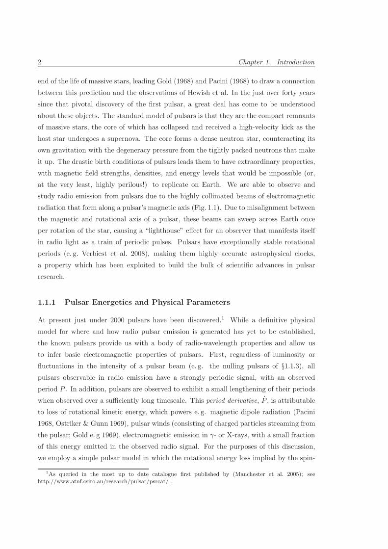
end of the life of massive stars, leading Gold (1968) and Pacini (1968) to draw a connection
between this prediction and the observations of Hewish et al. In the just over forty years
since that pivotal discovery of the first pulsar, a great deal has come to be understood
about these objects. The standard model of pulsars is that they are the compact remnants
of massive stars, the core of which has collapsed and received a high-velocity kick as the
host star undergoes a supernova. The core forms a dense neutron star, counteracting its
own gravitation with the degeneracy pressure from the tightly packed neutrons that make
it up. The drastic birth conditions of pulsars leads them to have extraordinary properties,
with magnetic field strengths, densities, and energy levels that would be impossible (or,
at the very least, highly perilous!) to replicate on Earth. We are able to observe and
study radio emission from pulsars due to the highly collimated beams of electromagnetic
radiation that form along a pulsar’s magnetic axis (Fig. 1.1). Due to misalignment between
the magnetic and rotational axis of a pulsar, these beams can sweep across Earth once
per rotation of the star, causing a “lighthouse” effect for an observer that manifests itself
in radio light as a train of periodic pulses. Pulsars have exceptionally stable rotational
periods (e. g. Verbiest et al. 2008), making them highly accurate astrophysical clocks,
a property which has been exploited to build the bulk of scientific advances in pulsar
research.
1.1.1 Pulsar Energetics and Physical Parameters
At present just under 2000 pulsars have been discovered.1 While a definitive physical
model for where and how radio pulsar emission is generated has yet to be established,
the known pulsars provide us with a body of radio-wavelength properties and allow us
to infer basic electromagnetic properties of pulsars. First, regardless of luminosity or
fluctuations in the intensity of a pulsar beam (e. g. the nulling pulsars of §1.1.3), all
pulsars observable in radio emission have a strongly periodic signal, with an observed
period P . In addition, pulsars are observed to exhibit a small lengthening of their periods
when observed over a sufficiently long timescale. This period derivative, P , is attributable
to loss of rotational kinetic energy, which powers e. g. magnetic dipole radiation (Pacini
1968, Ostriker & Gunn 1969), pulsar winds (consisting of charged particles streaming from
the pulsar; Gold e. g 1969), electromagnetic emission in γ- or X-rays, with a small fraction
of this energy emitted in the observed radio signal. For the purposes of this discussion,
we employ a simple pulsar model in which the rotational energy loss implied by the spin-
1As queried in the most up to date catalogue first published by (Manchester et al. 2005); seehttp://www.atnf.csiro.au/research/pulsar/psrcat/ .
1.1. Pulsars 3
Figure 1.1 A toy model of pulsar radio emission as described in the text, adapted fromLorimer & Kramer (2004). The magnetosphere of the pulsar may co-rotate within the lightcylinder, beyond which co-rotation would imply superluminous velocities. The radio beamis shown to originate from both magnetic poles along the open magnetic field lines. Tothe right, we indicate the signal seen by observers viewing the pulsar from three differentangles.
down observed in a pulsar is due entirely to magnetic dipole radiation.2 We can calculate
a pulsar’s spin-down luminosity (E) by relating the rotational kinetic energy loss to the
pulsar’s magnetic dipole radiation. Both of these quantities relate to the pulsar’s period
and period derivative, giving:
E =4π2IP
P 3=
2
3c3
(2π
P
)4(|m| sinα)2 (1.1)
(Lorimer & Kramer 2004), where |m| is the dipole’s magnetic moment, I is the pulsar’s
moment of inertia, and α is the angle between the magnetic and rotation axes. From this
we can determine the evolution of the rotation period of the pulsar with time:
P =dP
dt=
8π2
3Ic3· (|m| sinα)2 · P−1 . (1.2)
2The pulsar is assumed here to exist in a vacuum, ignoring other energy dissipation effects: mostnotably, those related to the pulsar magnetosphere. However, this model is the most basic (derived fromclassic electromagnetics) and is appropriate for most practical pulsar applications. It furthermore allowsthe derivation of a straight-forward estimator for characteristic age and magnetic field strength of pulsars.No comprehensive model to describe the behaviour of all pulsars has yet been established, but for a recentreview of such models, see Lyubarsky (2008).
4 Chapter 1. Introduction
We now adopt a commonly assumed value for the pulsar’s moment of inertia of I =
1038 kgm2 (Lorimer & Kramer 2004). On integrating equation 1.2 over time and assuming
that the pulsar’s period when it was formed is much less than its currently observed period,
we can define a characteristic age of the pulsar by the simple relation:
τc =P
(n− 1)P, (1.3)
Where n represents the braking index of the pulsar, which is defined by the energy loss in
the system, and relates the evolution of the first frequency derivative of the pulsar’s spin
to its period (ν ∝ νn). For the pure magnetic dipole braking scenario used here, n = 3.
Under the same pure magnetic dipole radiation scenario, the magnetic field strength
at a distance r relates to the magnetic dipole moment as B = 2|m| r−3. Equation 1.2
can thus be used to calculate the pulsar’s surface magnetic field strength at the pulsar’s
radius, R, also in terms of observables P and P :
Bsurf = sinα
(
3Ic3
8π2R6PP
)0.5
. (1.4)
In practice we use 3.2×10¹⁵√
PP Tesla, which is essentially a lower limit to Bsurf , setting
α = 90.
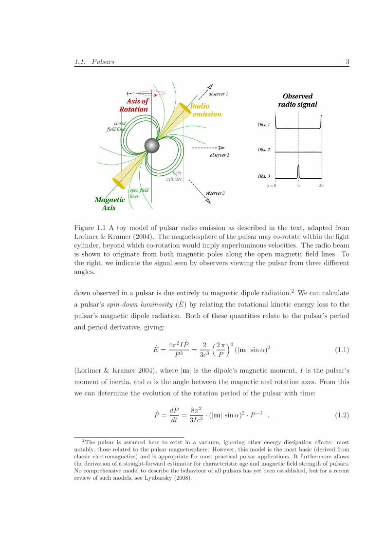
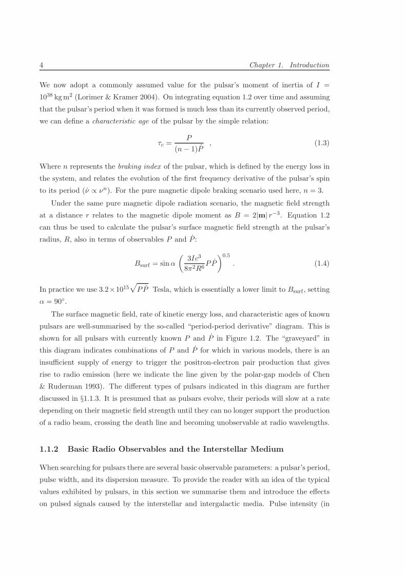
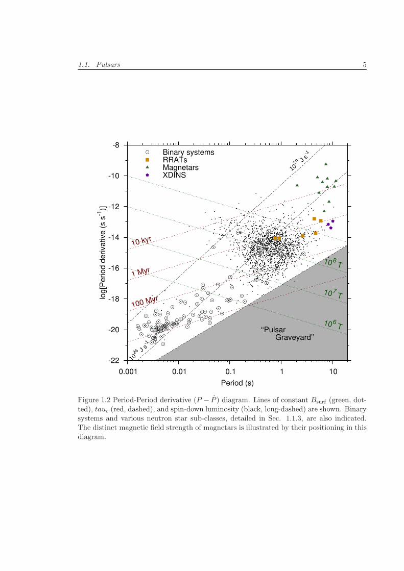
The surface magnetic field, rate of kinetic energy loss, and characteristic ages of known
pulsars are well-summarised by the so-called “period-period derivative” diagram. This is
shown for all pulsars with currently known P and P in Figure 1.2. The “graveyard” in
this diagram indicates combinations of P and P for which in various models, there is an
insufficient supply of energy to trigger the positron-electron pair production that gives
rise to radio emission (here we indicate the line given by the polar-gap models of Chen
& Ruderman 1993). The different types of pulsars indicated in this diagram are further
discussed in §1.1.3. It is presumed that as pulsars evolve, their periods will slow at a rate
depending on their magnetic field strength until they can no longer support the production
of a radio beam, crossing the death line and becoming unobservable at radio wavelengths.
1.1.2 Basic Radio Observables and the Interstellar Medium
When searching for pulsars there are several basic observable parameters: a pulsar’s period,
pulse width, and its dispersion measure. To provide the reader with an idea of the typical
values exhibited by pulsars, in this section we summarise them and introduce the effects
on pulsed signals caused by the interstellar and intergalactic media. Pulse intensity (in
1.1. Pulsars 5
-22
-20
-18
-16
-14
-12
-10
-8
0.001 0.01 0.1 1 10
log[P
eriod d
erivative (
s s
-1)]
Period (s)
Binary systemsRRATsMagnetarsXDINS
10 6 T
10 7 T
10 8 T
10 kyr
1 Myr
100 Myr
1029 J
s-1
1026 J
s-1
‘‘Pulsar Graveyard’’
Figure 1.2 Period-Period derivative (P − P ) diagram. Lines of constant Bsurf (green, dot-ted), tauc (red, dashed), and spin-down luminosity (black, long-dashed) are shown. Binarysystems and various neutron star sub-classes, detailed in Sec. 1.1.3, are also indicated.The distinct magnetic field strength of magnetars is illustrated by their positioning in thisdiagram.
6 Chapter 1. Introduction
0.0001
0.001
0.01
0.1
1
0.01 0.1 1 10 100 1000
Du
ty C
ycle
(w
/P)
Pulse width (ms)
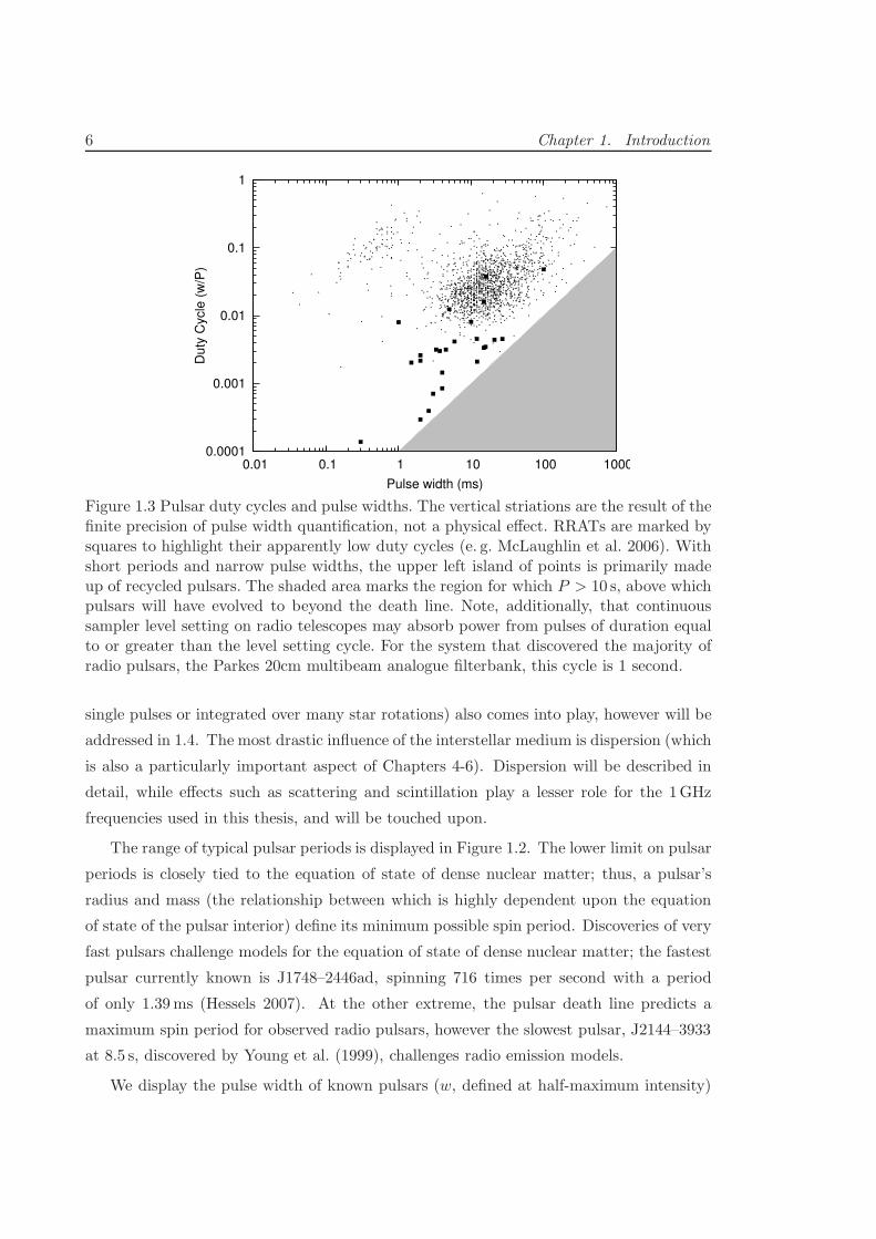
Figure 1.3 Pulsar duty cycles and pulse widths. The vertical striations are the result of thefinite precision of pulse width quantification, not a physical effect. RRATs are marked bysquares to highlight their apparently low duty cycles (e. g. McLaughlin et al. 2006). Withshort periods and narrow pulse widths, the upper left island of points is primarily madeup of recycled pulsars. The shaded area marks the region for which P > 10 s, above whichpulsars will have evolved to beyond the death line. Note, additionally, that continuoussampler level setting on radio telescopes may absorb power from pulses of duration equalto or greater than the level setting cycle. For the system that discovered the majority ofradio pulsars, the Parkes 20cm multibeam analogue filterbank, this cycle is 1 second.
single pulses or integrated over many star rotations) also comes into play, however will be
addressed in 1.4. The most drastic influence of the interstellar medium is dispersion (which
is also a particularly important aspect of Chapters 4-6). Dispersion will be described in
detail, while effects such as scattering and scintillation play a lesser role for the 1GHz
frequencies used in this thesis, and will be touched upon.
The range of typical pulsar periods is displayed in Figure 1.2. The lower limit on pulsar
periods is closely tied to the equation of state of dense nuclear matter; thus, a pulsar’s
radius and mass (the relationship between which is highly dependent upon the equation
of state of the pulsar interior) define its minimum possible spin period. Discoveries of very
fast pulsars challenge models for the equation of state of dense nuclear matter; the fastest
pulsar currently known is J1748–2446ad, spinning 716 times per second with a period
of only 1.39ms (Hessels 2007). At the other extreme, the pulsar death line predicts a
maximum spin period for observed radio pulsars, however the slowest pulsar, J2144–3933
at 8.5 s, discovered by Young et al. (1999), challenges radio emission models.
We display the pulse width of known pulsars (w, defined at half-maximum intensity)
1.1. Pulsars 7
in Fig. 1.3 against the duty cycle (w/P ) of pulsars. It is apparent here that the pulses
of pulsars occupy typically ∼10% of the star’s rotation. The “rotating radio transients”
with small duty cycles on this diagram will be discussed below in §1.1.3.
The intensity, frequency-dependent structure, and observed pulse width of pulsars
are all influenced by a number of effects (dispersion, refractive/diffractive scintillation,
scattering) caused by the cold, ionised plasmas that make up both the interstellar medium
(ISM), through which all celestial signals propagate before reaching an observer at Earth.
Any signal of extragalactic origin will also propagate through, and be influenced by, the
intergalactic medium (IGM) before passing into our Galaxy.
The existence of the ISM and IGM implies that the space between us and pulse-
emitting objects is not strictly a vacuum. In fact, the non-unity refractive index, n, of the
ISM causes light propagating through this medium to travel at a group velocity vg = c/n,
slower than the speed of light. As noted by Lorimer & Kramer (2004), the refractive index
of the interstellar medium is strongly dependent upon the plasma frequency of the ISM
and the frequency of the propagating light. The net effect of this is that a radio pulse
emitted by a celestial object experiences dispersion, resulting in an observable frequency-
dependent delay with time as exhibited in Fig. 1.4. The derivation of the cold plasma
dispersion relation in the ISM is summarised by Lorimer & Kramer (2004), and results in
a frequency-dependent lag with respect to a signal of infinite frequency:
∆t∞ =e2
2πmec· DM
f2; DM =
∫ d
0ne dl , (1.5)
f is the frequency of the emission, e is the elementary charge, and me is the mass of an
electron. The dispersion measure, DM, represents the integrated electron column density
along the line of sight from the observer to the emitter (at distance d). Below we use D ≡e2/(2πmec) ≃ 4.15× 10³ MHz2 pc−1 cm3 s. As implied by equation 1.5, higher frequencies
arrive before lower frequencies, as seen in Fig. 1.4. The DM is a direct observable, given a
pulse observed to arrive at two frequencies f1 and f2, at times t1 and t2, respectively:
∆t = t2 − t1 = D ·DM · (f−22 − f−2
1 ) . (1.6)
When creating a frequency-averaged time series for a pulsar, the data must be dedispersed,
that is, corrected for the frequency-dependent dispersion given by this equation. It is
implicit in Equation 1.5 that when the DM is measured for an object, one can infer a
distance to a Galactic emitter based on a model for the free electron distribution in the
Galaxy’s ISM. The current standard model used by pulsar astronomers is the “NE2001”
8 Chapter 1. Introduction
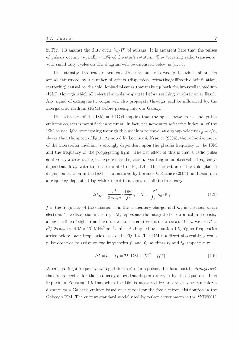
Figure 1.4 One pulse from the low-DM pulsar PSR J1456–6843. The lower panel shows aspectrogram, the power in greyscale as a function of frequency and the pulsar’s rotationalphase. The white lines trace DM = 8.6 pc cm−3. Several effects of the ISM are clear here:particularly the dispersion of the pulse and the frequency-dependent amplitude modulation(“scintles”) caused by wavefront distortions in the ISM. The upper panel shows the pulseprofile after dedispersion, integrated over the path traced by the white lines.
electron density model of Cordes & Lazio (2002). Pulse dispersion is generally a property
that is beneficial to surveys for pulsing objects; it creates a characteristic signal with which
to distinguish local (esp. man-made) signals from pulses of astrophysical origin. This will
be discussed further in Section 1.4 and is a central element to what makes the properties
of the discoveries in Chapter 6 so unexpected.
There are two remaining ISM effects which can influence pulsar measurements that
will play a role later in this thesis: the effects of pulse scattering, and scintillation. These
are mathematically and conceptually developed in detail by both Manchester & Taylor
(1977) and Lorimer & Kramer (2004) based on the “thin screen” model of Scheuer (1968)
(in which observed ISM effects are caused by a single screen positioned halfway between
observer and emitter). The reader is referred to those texts for details; we report only on
their derived results here.
Essentially, interstellar pulse broadening and scintillation both are caused by the fact
that the interstellar medium is both inhomogeneous and turbulent. A propagating wave-
front incident upon a scattering screen in the ISM will undergo random phase delays, the
magnitude of which are dependent upon the scale, a, of refractive index inhomogeneities
(that is, electron density variations, ∆ne). These delays cause several effects. First, they
1.1. Pulsars 9
will induce a frequency-dependent scatter broadening of a pulse, causing a delta-function
pulse to have an asymmetric tail. Furthermore, interference induced by the wavefront
distortions will cause constructive and destructive interference leading to frequency- and
time-dependent flux variations (scintillation) with a characteristic timescale and band-
width, depending on the nature of the scattering screen and the relative velocities of the
pulsar, Earth, and screen. These effects can have dramatic influences on an observation,
particularly when the characteristic bandwidth of the scintillation is equal to the observing
bandwidth. These effects are typically stronger for low-dispersion measure/nearby pulsars
(e. g. Fig. 1.4), and can cause a newly discovered pulsar to not be seen in subsequent
observations if it was discovered near a caustic peak of scintillation.
For the thin screen model considered by the texts noted above, the scattering timescale,
τs can be approximated by:
τs =e4
4π2m2e
∆n2ea
d2 f−4 . (1.7)
Here, τs is in milliseconds, and the observing frequency f is in units of GHz. It is clear that
the scale and position of inhomogeneities influence the effects of the ISM on the signal. It
is often assumed (and, despite the relation below, holds in observations for some objects)
that the turbulence of the ISM obeys a Kolmogorov energy spectrum (Kolmogorov 1941),
for which τs ∝ f−4.4. The distance dependence indicates that τs scales with dispersion
measure. In fact, although there is significant scatter, Bhat et al. (2004) give a relation
that is useful when considering the design of pulsar surveys (§1.4.1,§5.2.2):
log10τs = −6.46 + 0.154 log10(DM) + 1.07 [log10 (DM)]2 − 3.86 log10 (f) (1.8)
This relationship indicates the ability of pulsars observations to assess the applicability
of turbulence models to the ISM, indicating that on average the frequency dependence of
scattering is actually closer to τs ∝ f−3.86.
1.1.3 Pulsar Varieties
The vast majority of electromagnetically-emitting neutron stars occupy the island of ra-
dio pulsars with intermediate rotational speeds visible in Figure 1.2. However, there are
several sub-varieties of neutron stars, segregated both by differences in physically under-
stood properties, and by observed (not always yet understood) differences in behaviour. In
radio bands, the behavioural sub-groups most relevant to this thesis are: millisecond pul-
sars, nulling pulsars, modulated and giant-bursting pulsars, and rotating radio transients.
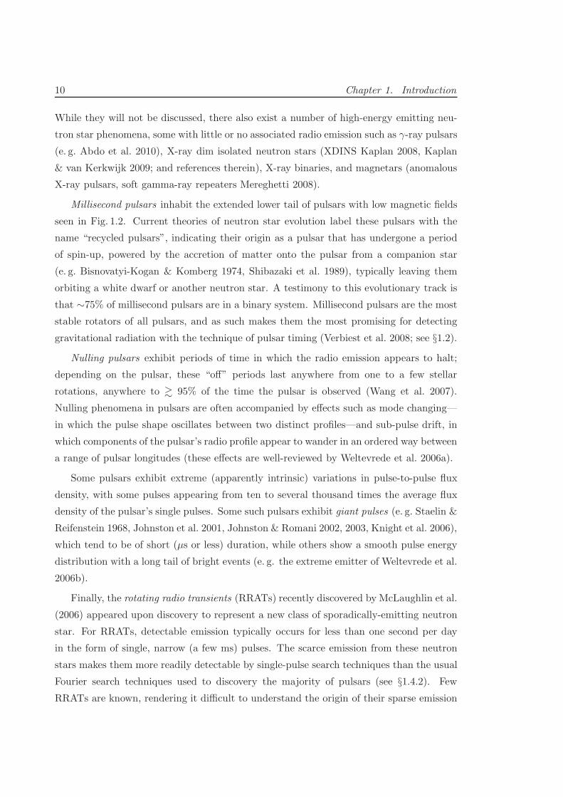
10 Chapter 1. Introduction
While they will not be discussed, there also exist a number of high-energy emitting neu-
tron star phenomena, some with little or no associated radio emission such as γ-ray pulsars
(e. g. Abdo et al. 2010), X-ray dim isolated neutron stars (XDINS Kaplan 2008, Kaplan
& van Kerkwijk 2009; and references therein), X-ray binaries, and magnetars (anomalous
X-ray pulsars, soft gamma-ray repeaters Mereghetti 2008).
Millisecond pulsars inhabit the extended lower tail of pulsars with low magnetic fields
seen in Fig. 1.2. Current theories of neutron star evolution label these pulsars with the
name “recycled pulsars”, indicating their origin as a pulsar that has undergone a period
of spin-up, powered by the accretion of matter onto the pulsar from a companion star
(e. g. Bisnovatyi-Kogan & Komberg 1974, Shibazaki et al. 1989), typically leaving them
orbiting a white dwarf or another neutron star. A testimony to this evolutionary track is
that ∼75% of millisecond pulsars are in a binary system. Millisecond pulsars are the most
stable rotators of all pulsars, and as such makes them the most promising for detecting
gravitational radiation with the technique of pulsar timing (Verbiest et al. 2008; see §1.2).
Nulling pulsars exhibit periods of time in which the radio emission appears to halt;
depending on the pulsar, these “off” periods last anywhere from one to a few stellar
rotations, anywhere to & 95% of the time the pulsar is observed (Wang et al. 2007).
Nulling phenomena in pulsars are often accompanied by effects such as mode changing—
in which the pulse shape oscillates between two distinct profiles—and sub-pulse drift, in
which components of the pulsar’s radio profile appear to wander in an ordered way between
a range of pulsar longitudes (these effects are well-reviewed by Weltevrede et al. 2006a).
Some pulsars exhibit extreme (apparently intrinsic) variations in pulse-to-pulse flux
density, with some pulses appearing from ten to several thousand times the average flux
density of the pulsar’s single pulses. Some such pulsars exhibit giant pulses (e. g. Staelin &
Reifenstein 1968, Johnston et al. 2001, Johnston & Romani 2002, 2003, Knight et al. 2006),
which tend to be of short (µs or less) duration, while others show a smooth pulse energy
distribution with a long tail of bright events (e. g. the extreme emitter of Weltevrede et al.
2006b).
Finally, the rotating radio transients (RRATs) recently discovered by McLaughlin et al.
(2006) appeared upon discovery to represent a new class of sporadically-emitting neutron
star. For RRATs, detectable emission typically occurs for less than one second per day
in the form of single, narrow (a few ms) pulses. The scarce emission from these neutron
stars makes them more readily detectable by single-pulse search techniques than the usual
Fourier search techniques used to discovery the majority of pulsars (see §1.4.2). Few
RRATs are known, rendering it difficult to understand the origin of their sparse emission
1.2. Pulsar Timing and Timing Arrays 11
(Chapter 4 addresses this topic). Several observed properties appear to make RRATs
distinct from the general pulsar population, including their small duty cycles (Fig. 1.3).
Recent measurements of RRAT periods and period derivatives have led to the conclusions
that Bsurf for RRATs is distinctly higher than average pulsar magnetic fields, and RRAT
periods are statistically longer than those of regularly-emitting pulsars, seeming to further
differentiate the RRATs from the typical pulsar population (McLaughlin et al. 2009).
1.2 Pulsar Timing and Timing Arrays
As noted above, the regularity of pulsars’ rotations make them not unlike precise natu-
rally occurring clocks. This property has yielded the technique of “pulsar timing,” which
involves the measurement and prediction of a pulsar’s pulse arrival times. Pulsar tim-
ing employs models for Earth’s motion relative to the pulsar (that is, due to its move-
ment around the Solar System barycentre), for the ISM effects described in 1.1.2, and
for the pulsar itself (e. g. P , P , binary motion) based on previous observations of the
pulsar. The most stable millisecond pulsars have pulse arrival times stable to the order
of < 10−6 seconds over timescales from days to decades (e. g Verbiest et al. 2008). After
correction for modelled effects, any physics or systematics that are unaccounted for will
manifest structure in the pulsar’s timing residuals, which are the actual pulse arrival times
relative to the predicted times of arrival. It is in the post-model-fit timing residuals that
one may search for subtle inaccuracies in the models, or for unmodelled influences on the
pulsar, Earth, or the intervening space between.
Greater sensitivity to spatially-correlated effects arises with the concurrent monitoring
of multiple pulsars in what is termed a pulsar timing array (PTA: this term was coined by
Romani 1989, although first rigorously employed by Hellings & Downs 1983 to put limits
on gravitational radiation. Foster & Backer 1990 first detailed other physical targets that a
PTA could explore). PTAs aim to detect correlated offsets in the timing residuals of pulsars
spread across the celestial sphere, forming a measurement tool akin to an accelerometer
for Earth within space-time. Targeted effects include errors in Earth’s time standards
(currently maintained by atomic clocks), errors in solar system ephemerides (planet mass
errors, which would produce strongly correlated residuals along the ecliptic, or unidentified
solar system bodies Champion et al. 2010), and the ultimate target of pulsar astronomy,
gravitational waves (Detweiler 1979).
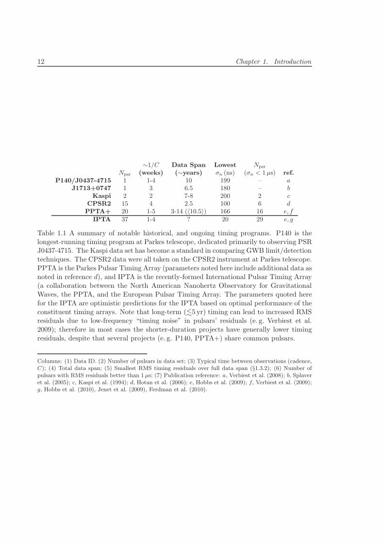
While there are many efforts in pulsar timing around the globe, there are several
projects and pulsars of particular note. Relevant timing parameters of these projects are
summarised in Table 1.1.
12 Chapter 1. Introduction
∼1/C Data Span Lowest Npsr
Npsr (weeks) (∼years) σn (ns) (σn < 1µs) ref.P140/J0437-4715 1 1-4 10 199 – a
J1713+0747 1 3 6.5 180 – bKaspi 2 2 7-8 200 2 c
CPSR2 15 4 2.5 100 6 dPPTA+ 20 1-5 3-14 (〈10.5〉) 166 16 e, f
IPTA 37 1-4 ? 20 29 e, g
Table 1.1 A summary of notable historical, and ongoing timing programs. P140 is thelongest-running timing program at Parkes telescope, dedicated primarily to observing PSRJ0437-4715. The Kaspi data set has become a standard in comparing GWB limit/detectiontechniques. The CPSR2 data were all taken on the CPSR2 instrument at Parkes telescope.PPTA is the Parkes Pulsar Timing Array (parameters noted here include additional data asnoted in reference d), and IPTA is the recently-formed International Pulsar Timing Array(a collaboration between the North American Nanohertz Observatory for GravitationalWaves, the PPTA, and the European Pulsar Timing Array. The parameters quoted herefor the IPTA are optimistic predictions for the IPTA based on optimal performance of theconstituent timing arrays. Note that long-term (.5 yr) timing can lead to increased RMSresiduals due to low-frequency “timing noise” in pulsars’ residuals (e. g. Verbiest et al.2009); therefore in most cases the shorter-duration projects have generally lower timingresiduals, despite that several projects (e. g. P140, PPTA+) share common pulsars.
Columns: (1) Data ID. (2) Number of pulsars in data set; (3) Typical time between observations (cadence,C); (4) Total data span; (5) Smallest RMS timing residuals over full data span (§1.3.2); (6) Number ofpulsars with RMS residuals better than 1µs; (7) Publication reference: a, Verbiest et al. (2008); b, Splaveret al. (2005); c, Kaspi et al. (1994); d, Hotan et al. (2006); e, Hobbs et al. (2009); f, Verbiest et al. (2009);g, Hobbs et al. (2010), Jenet et al. (2009), Ferdman et al. (2010).
1.3. Gravitational Wave Astronomy 13
1.3 Gravitational Wave Astronomy
Gravitational radiation is a direct prediction of Einstein’s space-time metric equations of
general relativity: a gravitational wave (GW) is a propagating quadrupolar fluctuation in
the curvature of space-time that is produced when a mass is accelerated, mathematically
analogous to the electromagnetic waves produced by an accelerated electron. No gravita-
tional waves have yet been detected, however the first indirect observational evidence for
GWs arose from the timing of the binary neutron star PSR B1913+16 (Hulse & Taylor
1975) by (Taylor & Weisberg 1982), who showed that the system is losing orbital energy
at precisely the rate expected from the energy lost from the system due to GW emission
(a discovery which resulted in the Nobel Prize for physics!).
As a gravitational wave (GW) propagates, it creates small distortions in space-time
perpendicular to its propagation axis. Provided the wave is within the pulsar timing
band, such a wave is theoretically directly detectable by PTAs through its quadrupolar
fingerprint left as a correlated signal in the array. Given many sources of unresolved
GWs, they will produce a stochastic GW background (GWB) that is detectable in PTA
data through its correlated signature in timing residuals (Hellings & Downs 1983). Given
a well-timed, individual pulsar, limits may be placed on the presence and strength of
gravitational radiation or a GWB, however a definitive detection cannot be separated
from other effects.
1.3.1 Pulsar-detectable Gravitational Wave Sources
Pulsar timing is sensitive to unpredicted changes in the Earth’s movement on timescales
between the length of sustained pulsar observations (some timing data sets now reach
up to several decades), and the cadence of pulsar observations, at most typically one
every two weeks. Consequently, pulsar timing data have sensitivity to the low-frequency
(nHz . fgw . µHz) gravitational wave spectrum, complementary to gravitational wave
detectors such as the Laser Interferometer Gravitational Wave Observatory (“LIGO”) and
the planned Laser Interferometer Space Antenna (“LISA”). The gravitational radiation
spectrum, various theoretical sources and limits of current and future GW detectors are
summarised in Fig. 1.5.
Theoretical sources of gravitational wave emission in the pulsar timing band include
GWBs from primordial intermediate-mass black holes (Saito & Yokoyama 2009), cosmic
strings (Caldwell et al. 1996, Damour & Vilenkin 2005), and tensor perturbations from the
rapid expansion of the inflation epoch in the early Universe (Maggiore 2000, Grishchuk
14 Chapter 1. Introduction
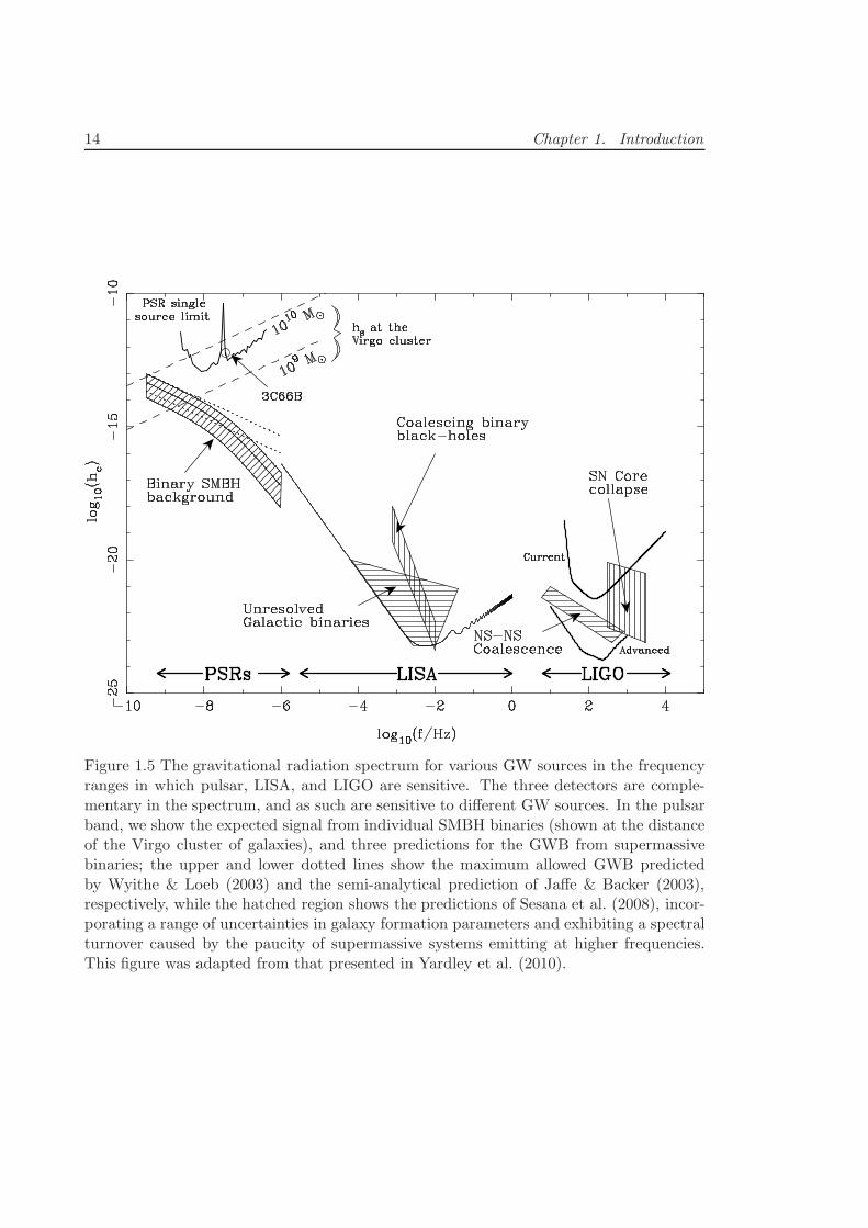
Figure 1.5 The gravitational radiation spectrum for various GW sources in the frequencyranges in which pulsar, LISA, and LIGO are sensitive. The three detectors are comple-mentary in the spectrum, and as such are sensitive to different GW sources. In the pulsarband, we show the expected signal from individual SMBH binaries (shown at the distanceof the Virgo cluster of galaxies), and three predictions for the GWB from supermassivebinaries; the upper and lower dotted lines show the maximum allowed GWB predictedby Wyithe & Loeb (2003) and the semi-analytical prediction of Jaffe & Backer (2003),respectively, while the hatched region shows the predictions of Sesana et al. (2008), incor-porating a range of uncertainties in galaxy formation parameters and exhibiting a spectralturnover caused by the paucity of supermassive systems emitting at higher frequencies.This figure was adapted from that presented in Yardley et al. (2010).
1.3. Gravitational Wave Astronomy 15
2005, Boyle & Buonanno 2008).
The strongest expected sources of gravitational radiation for pulsar timing come from
the most massive compact objects in the Universe: supermassive black holes (mass>106 M⊙,
hereafter SMBHs), which reside at the center of nearly all massive galaxies. SMBHs will
produce the strongest gravitational waves in the Universe when in a closely bound binary
system with another SMBH, emitting gravitational waves with a period half of the sys-
tem’s orbital period. Therefore, PTAs have sensitivity to these systems when the orbital
period of the binary is within the time scale of the pulsar timing experiment: that is, when
the orbital separation is r ≪ 10 pc (for more details see §2.3). The expected number of
individual binary systems detectable by pulsar timing arrays was explored by Sesana et al.
(2009). In a Universe built up by the hierarchical merging of galaxies, a stochastic GWB
from many SMBH binary systems is also expected, with a strength and spectral form de-
pendent upon the mass, number density, and cosmological distribution of binary systems
in the Universe (which, in turn, have a strong dependence on the parameters of galaxy and
SMBH growth, such as the time-dependent merger rate of galaxies, the post-merger inspi-
ral timescale for SMBHs, and the contribution of accretion versus mergers to SMBH mass
growth). This implies a close link between pulsar timing and galaxy evolution, through
which limits from pulsar timing on the astrophysical gravitational wave background can
be used to constrain models of galaxy formation. Until a background is detected, pulsar
timing studies rely on galaxy evolution models to give predictions for the amplitude and
spectral form of the GW signals; however with very strong limits on or a detection of
the GWB, pulsar timing will be able to constrain various facets of galaxy evolution that
are otherwise difficult to derive through electromagnetic observation. The predicted form
of the astrophysical GWB has been explored in basic hierarchical-merging contexts by
Rajagopal & Romani (1995), Jaffe & Backer (2003), Wyithe & Loeb (2003), Enoki et al.
(2004), and expanded for the inclusion of uncertainties in several galaxy formation parame-
ters by Sesana et al. (2008). However, a major—and potentially detrimental—uncertainty
in these models remains in the observationally unconstrained inspiral timescale for SMBH
binaries after a galaxy merger, which the predictive models generally neglect. It is cur-
rently not known whether there is sufficient fuel for orbital energy dissipation during
SMBH binary inspiral for the SMBHs to coalesce within a Hubble time, giving rise to the
possibility of “stalled” SMBH binary systems that remain at orbital separations beyond
those detectable by pulsar timing. This is colloquially termed the “last parsec problem”,
referring to the ineffectiveness of energy dissipation mechanisms to shrink a binary below
separations of ∼1 pc (Begelman et al. 1980, Merritt & Milosavljevic 2005).
16 Chapter 1. Introduction
1.3.2 Gravitational Wave Signals and Timing Sensitivity
Here we review the mathematical representation of the signal from gravitational wave
backgrounds and individual SMBH binary sources, and the sensitivity of pulsar timing
to GW emission. The fractional contribution of the GWB to the energy density of the
Universe in a logarithmic frequency interval can be expressed as:
Ωgw(f) =2π2
3H20
f3Sh(f) ; Sh(f) =hc(f)
2
f, (1.9)
where Sh(f) represents the total power spectral density of gravitational waves at frequency
f (using the “one-sided” convention of Jaffe & Backer 2003), and hc(f) represents the
characteristic strain spectrum of the GWB. For most predictions of gravitational wave
background, the characteristic strain follows a power law with frequency, as
hc(f) = A
(
f
f0
)α
, (1.10)
with amplitude A, and spectral index α at a normalising frequency f0 = 1yr−1. Most
backgrounds can be described in this way; e. g for primordial GWs, α ranges −0.8 to −1.0
with amplitudes 10−17 < A < 10−15, while for the GWB from SMBH binaries, predictions
typically find that α = −2/3 and 10−16 < A < 10−14.
The astrophysical background of supermassive binaries, as noted above, is defined by
the density and distribution of SMBHs in the Universe. This is well-illustrated by the
simple formulation for the characteristic strain spectrum of SMBH binaries given by Jaffe
& Backer (2003):
hc(f)2 = f N(z, f,m1,m2)
∫
h2s(z, f,m1,m2) dz dm1 dm2 . (1.11)
Here, z is the cosmological redshift of the source (analogous to distance), m1 and m2 are
the masses of the constituent black holes, N(z, f,m1,m2) represents the number density
of systems per f,m1,m2, and redshift bin, and hs is the strain contributed by one binary
system:
hs = 4
√
2
5
(GM)5/3
c4D· (2π/P )2/3 (1.12)
(Peters & Mathews 1963, Thorne 1989), where M = (m1m2M−1/3)3/5 is the chirp mass
of a binary system, and D is the distance to the object. Note how the strain scales with
distance at hs ∝ D−1 (that is, it is not analagous to e. g. a flux density).
Given the steep spectrum predicted for all GWBs in the pulsar timing band, the
1.4. Pulsar Searches and Fast-Transient Radio Astronomy 17
most stringent limits set by pulsar timing on GWBs are at the lowest frequency—that is,
timing arrays are most sensitive to these backgrounds at frequencies 1/T , where T is the
time span of the arrays’ observations. In fact, pulsar timing’s sensitivity to gravitational
waves depends on a number of factors, also including the accuracy of a pulsar’s timing
model over the span of the experiment (timing precision is quantified by the root-mean-
squared of the timing residuals, σn), the cadence and regularity of observations, and for
gravitational wave detection with pulsar timing arrays, the sensitivity depends on the
number of pulsars in the array and their distribution on the sky. The sensitivity to
gravitational wave backgrounds of α = −2/3 was derived by Jenet et al. (2005) for pulsar
timing arrays; they find that an array of Npsr pulsars can detect a gravitational wave
background to a significance of S ∝√
(Npsr(Npsr − 1)) (in noise-dominated data as we
currently have, however S ∝√
Npsr when S becomes significant). They furthermore derive
the dependence of the lowest detectable A on PTA observing parameters (or, for the case
of single pulsars, the dependence of the limit placed on A), finding A ∝ σn T−5/3N−1/2,
where N is the number of observations for each pulsar in the array. We can see here that
data sets of long duration provide significant improvements in pulsar timing’s sensitivity
to the supermassive binary GWB, and further critical improvements come with a better
understanding of long-term intrinsic pulsar instabilities and observing hardware/software
systematics; both of these contribute to a larger σn of a pulsar’s timing residuals.
Because of data-fitting procedures performed during timing, the sensitivity of pulsar
timing arrays to single sources of gravitational radiation is not straight forward to define.
However, it has been formally calculated for pulsars in the Parkes Pulsar Timing Array
by Yardley et al. (2010), whose single-source sensitivity curve is shown in Fig. 1.5 as the
“PSR single source limit”.
1.4 Pulsar Searches and Fast-Transient Radio Astronomy
1.4.1 Considerations in Pulsar Survey Design
As one can infer by pulsar’s fast periods, short impulse durations, and the need to correct
for a pulse’s dispersion (§1.1.2), the systems employed for observing pulsars are highly
specialised.
An ideal pulsar search system will sample the sky at intervals of tsamp . 1ms in
individual frequency channels of width b over a total bandwidth B. Blind surveys must
search a range of DMs, and aim to minimize b and tsamp such that the observed width of
a pulse with intrinsic width wint is usually dominated by τs (Eq.s 1.7, 1.8), rather than
18 Chapter 1. Introduction
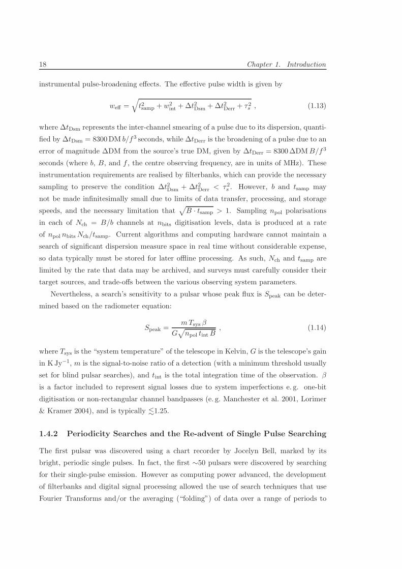
instrumental pulse-broadening effects. The effective pulse width is given by
weff =√
t2samp + w2int +∆t2Dsm +∆t2Derr + τ2s , (1.13)
where ∆tDsm represents the inter-channel smearing of a pulse due to its dispersion, quanti-
fied by ∆tDsm = 8300DM b/f3 seconds, while ∆tDerr is the broadening of a pulse due to an
error of magnitude ∆DM from the source’s true DM, given by ∆tDerr = 8300∆DMB/f3
seconds (where b, B, and f , the centre observing frequency, are in units of MHz). These
instrumentation requirements are realised by filterbanks, which can provide the necessary
sampling to preserve the condition ∆t2Dsm + ∆t2Derr < τ2s . However, b and tsamp may
not be made infinitesimally small due to limits of data transfer, processing, and storage
speeds, and the necessary limitation that√
B · tsamp > 1. Sampling npol polarisations
in each of Nch = B/b channels at nbits digitisation levels, data is produced at a rate
of npol nbitsNch/tsamp. Current algorithms and computing hardware cannot maintain a
search of significant dispersion measure space in real time without considerable expense,
so data typically must be stored for later offline processing. As such, Nch and tsamp are
limited by the rate that data may be archived, and surveys must carefully consider their
target sources, and trade-offs between the various observing system parameters.
Nevertheless, a search’s sensitivity to a pulsar whose peak flux is Speak can be deter-
mined based on the radiometer equation:
Speak =mTsys β
G√
npol tintB, (1.14)
where Tsys is the “system temperature” of the telescope in Kelvin, G is the telescope’s gain
in KJy−1, m is the signal-to-noise ratio of a detection (with a minimum threshold usually
set for blind pulsar searches), and tint is the total integration time of the observation. β
is a factor included to represent signal losses due to system imperfections e. g. one-bit
digitisation or non-rectangular channel bandpasses (e. g. Manchester et al. 2001, Lorimer
& Kramer 2004), and is typically .1.25.
1.4.2 Periodicity Searches and the Re-advent of Single Pulse Searching
The first pulsar was discovered using a chart recorder by Jocelyn Bell, marked by its
bright, periodic single pulses. In fact, the first ∼50 pulsars were discovered by searching
for their single-pulse emission. However as computing power advanced, the development
of filterbanks and digital signal processing allowed the use of search techniques that use
Fourier Transforms and/or the averaging (“folding”) of data over a range of periods to
1.4. Pulsar Searches and Fast-Transient Radio Astronomy 19
Channelised(e.g. filterbank)
Data
FFT
Cand. List(time, filter, DM)
FFA
Harmonic
sumsDiagnostic
plots
Determine
best cands
(max DM, P)
Manual
inspectionDispersion
trial
Pre-set thresholds
Filter
trial?
Apply filter
Cand. list(P, DM)
Another
DM trial?Event
searchY
N
Y
N
N
Y
Periodicity
search
Single pulse
search
(a)
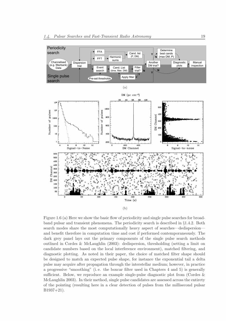
(b)
Figure 1.6 (a) Here we show the basic flow of periodicity and single pulse searches for broad-band pulsar and transient phenomena. The periodicity search is described in §1.4.2. Bothsearch modes share the most computationally heavy aspect of searches—dedispersion—and benefit therefore in computation time and cost if performed contemporaneously. Thedark grey panel lays out the primary components of the single pulse search methodsoutlined in Cordes & McLaughlin (2003): dedispersion, thresholding (setting a limit oncandidate numbers based on the local interference environment), matched filtering, anddiagnostic plotting. As noted in their paper, the choice of matched filter shape shouldbe designed to match an expected pulse shape, for instance the exponential tail a deltapulse may acquire after propagation through the interstellar medium; however, in practicea progressive “smoothing” (i. e. the boxcar filter used in Chapters 4 and 5) is generallysufficient. Below, we reproduce an example single-pulse diagnostic plot from (Cordes &McLaughlin 2003). In their method, single pulse candidates are assessed across the entiretyof the pointing (resulting here in a clear detection of pulses from the millisecond pulsarB1937+21).
20 Chapter 1. Introduction
allow increased sensitivity to the periodic signals exhibited by pulsars. Today, a typical
pulsar search proceeds as outlined in the left panel of Figure 1.6, beginning with the
dedispersion of multi-channel data into a band-integrated time series for each DM trial
(with trial step intervals usually chosen to maintain ∆tDerr . 2∆tDsm for pulsars with a
DM between two steps). The time series are then used to perform periodicity searches
(e. g. using the Fast Fourier Transform, Brigham 1974, Ransom et al. 2002, or a fast
folding algorithm, Staelin 1969), performing harmonic summing of Fourier components to
increase sensitivity to pulsars of small duty cycle (Ransom et al. 2002). Such techniques
have allowed the discovery of great numbers of pulsars, many that would have been too
weak to discover by their single pulses alone.
However, given the specifications of the pulsar search systems outlined above, it is
not surprising that pulsar data and observing systems are ideally suited for performing
searches for single-event, short-duration pulses from not only neutron stars, but other
miriad other possible celestial sources. Single celestial impulses will, too, be dispersed,
requiring fast sampling and narrow sub-bands with which to correct for dispersion effects.
As such, past pulsar surveys represent one of the few historical records of the sky capable of
detecting transient radio events of duration ≪1 second, while new surveys present further
search opportunities, and (given sufficient computing power) the chance to find events in
real-time, allowing prompt follow-up observations.
In the past decade astronomers have begun to recognise this fact, returning to archival
pulsar surveys that have already been rigorously searched for periodic signals, and applying
new algorithms to search for transient, one-off pulses that would have been missed by
Fourier search techniques; Fourier transform searches are insensitive to single bursts of
emission, and become less sensitive to some periodic sources due to to erratic or sparse
emission, short duty cycles, and long rotation periods (the latter due to low-frequency
noise in the data, e. g. Deneva et al. 2009). While the first blind searches for single pulses
began a number of years prior to its publication, Cordes & McLaughlin (2003) first laid
out the known sources of transient radio emission, considering a “transient phase space”
that exhibits these phenomena (Fig. 1.7), and developing a set of standard methodologies
for single pulse searching (see section §4.1 for a more complete review of blind single pulse
searches). The primary features in the Cordes & McLaughlin search methods are outlined
and discussed in Figure 1.6.
It is now recognised that there may be many transient phenomena detectable in pulsar
surveys that, if detected, may provide insight into a variety of emission sources. These are
reviewed below.
1.4. Pulsar Searches and Fast-Transient Radio Astronomy 21
log
[ Spe
akD
2 (Jy
kpc
2 ) ]
log [ f wint (GHz s) ]
-5
0
5
10
-10 -5 0 5 10
TB=1040K 1030 K 1020 K
1010 K 100 K
COHERENT
INCOHERENTRRATs
Pulsars
B0656+14
Crabgiant pulses
Crabnano-pulses B0540-69
giant pulses
AG
N
Type II, IIISolar Bursts
OH Masers
UV CetiAD Leo
Brown DwarfLP944-20Jupiter
LorimerBurst
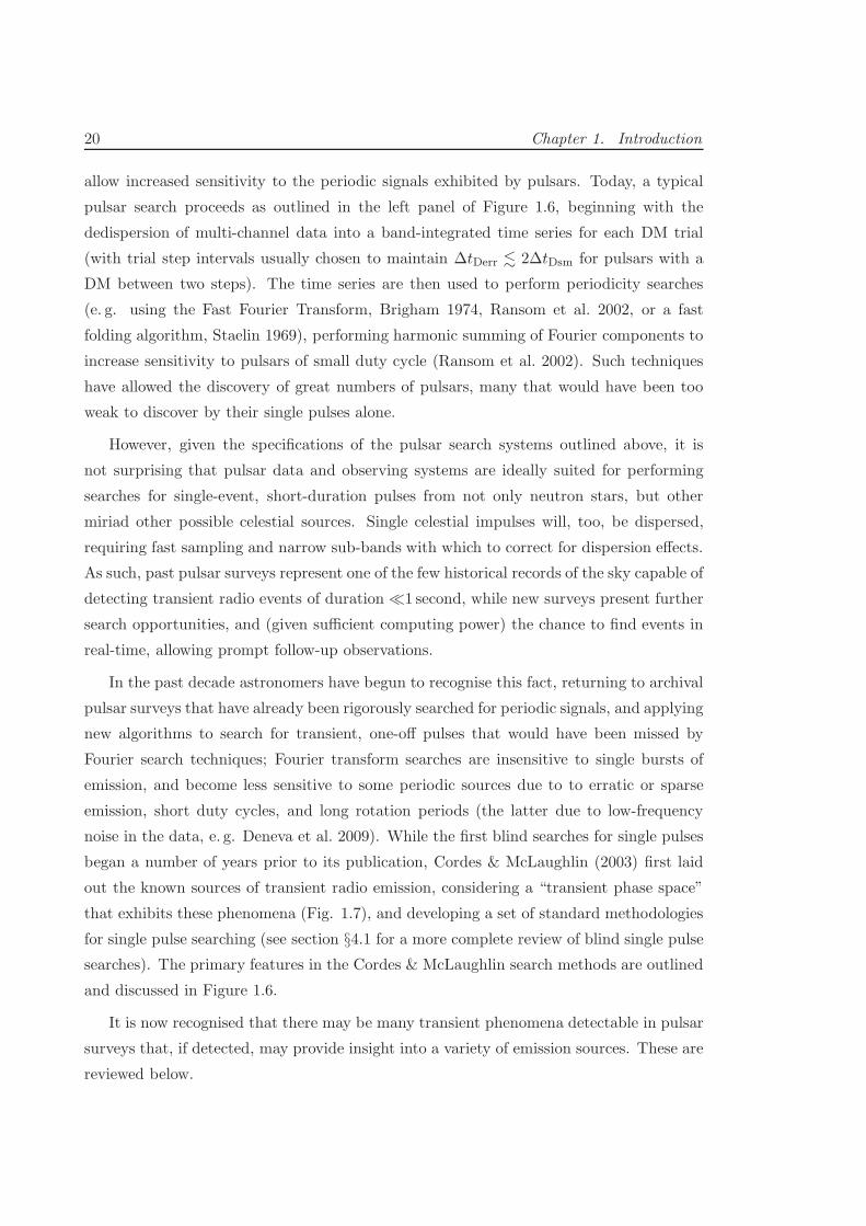
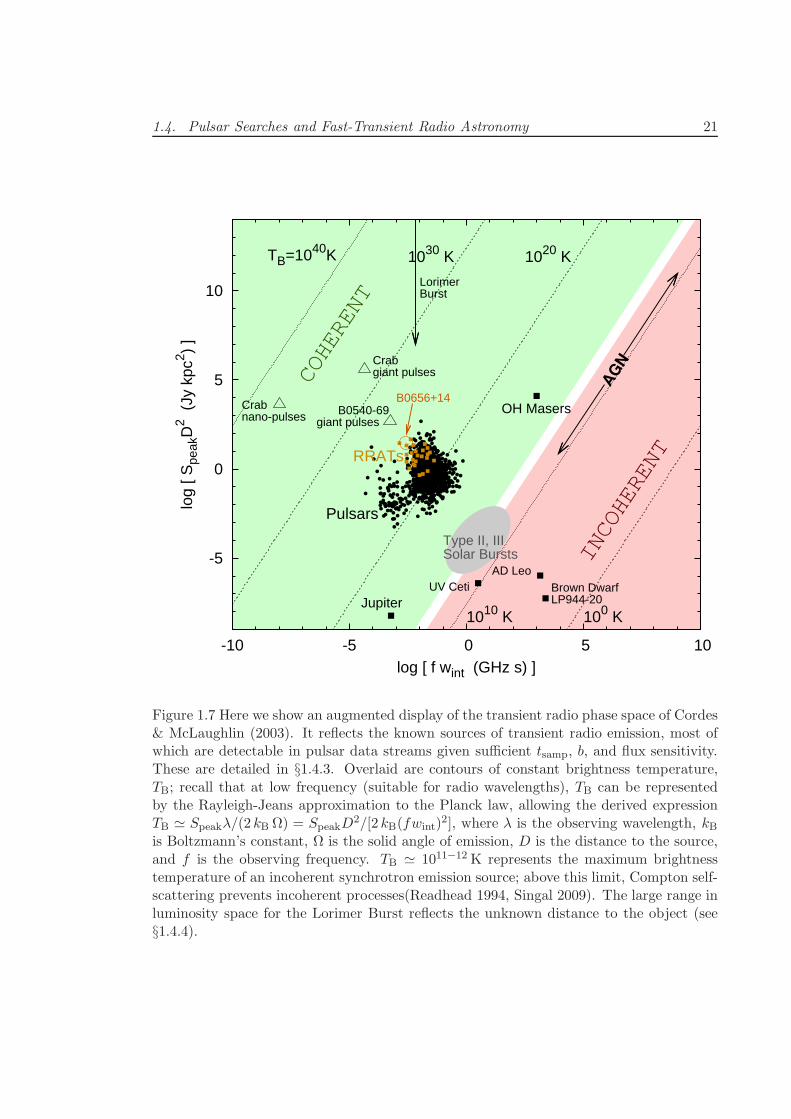
Figure 1.7 Here we show an augmented display of the transient radio phase space of Cordes& McLaughlin (2003). It reflects the known sources of transient radio emission, most ofwhich are detectable in pulsar data streams given sufficient tsamp, b, and flux sensitivity.These are detailed in §1.4.3. Overlaid are contours of constant brightness temperature,TB; recall that at low frequency (suitable for radio wavelengths), TB can be representedby the Rayleigh-Jeans approximation to the Planck law, allowing the derived expressionTB ≃ Speakλ/(2 kB Ω) = SpeakD
2/[2 kB(fwint)2], where λ is the observing wavelength, kB
is Boltzmann’s constant, Ω is the solid angle of emission, D is the distance to the source,and f is the observing frequency. TB ≃ 1011−12 K represents the maximum brightnesstemperature of an incoherent synchrotron emission source; above this limit, Compton self-scattering prevents incoherent processes(Readhead 1994, Singal 2009). The large range inluminosity space for the Lorimer Burst reflects the unknown distance to the object (see§1.4.4).
22 Chapter 1. Introduction
1.4.3 Known Sources of Fast Transient Radio Emission
It is clear in Figure 1.7 that there are only a handful of known classes of radio transients.
We note that above TB ∼ 1015 K, this phase space has until recently been restricted to
periodicity-focussed searches using Fourier techniques.
Pulsars form a fairly compact island on this diagram. Several neutron-star related
objects, all of which have distinctive single-pulse emission, have isolated positions; for
instance, pulsars such as the Crab, which in its integrated emission lies within the pulsar
island, emits giant (105 Jy) single pulses as well as high-intensity bursts of nanosecond
duration. High pulse-to-pulse modulation and periodic nulling represent other types of
signal variance observed in the single pulse emission of some pulsars (e.g. Herfindal &
Rankin 2007, Kramer et al. 2006). Such neutron star-related phenomena promise insights
into the localisation and power source of radio pulsar emission. Single pulse searches
have the ability to discover extreme examples of these sources, and may serve to reveal a
bridging population or define a distinction between steadily-emitting pulsars and pulsars
with excessive nulls. This could help reveal whether the rotating radio transients of §1.1.3are (in physical mechanism) just extreme examples of nulling pulsars (see Chap. 4) or
distant, modulated pulsars, such as radio pulsar B0656+14, which has a lognormal pulse
energy distribution with a high-energy tail that sets it apart from typical pulse energy
distributions. This pulsar was found to have a single-pulse energy distribution with a long
high-energy tail, leading to the supposition of Weltevrede et al. (2006b) that the pulsar
is a source which, if it were more distant from Earth (thus making its average emission
undetectable), might be observed as an RRAT.
Non-neutron star transient phenomena that exist in the transient sky, however were not
discovered through pulsar-data searches, include active galactic nuclei, which exhibit
intrinsic intermediate-duration flares (e. g. Aller et al. 1985, Kawai et al. 1991, Robson et al.
1993) as well as intra-day variability caused by interstellar scintillation (see discussion
on AGN variability in §3.3). Flares have been observed to arise on second- to hour-
long timescales from a number of sources: for instance brown dwarfs, giving us insight
into the magnetic activity in these stars (Berger et al. 2001), active stars (e. g. UV
Ceti, AD Leo, and several others Jackson et al. 1989)—revealing cycles possibly similar
to those of the sun—and even Jupiter (Goldreich & Lynden-Bell 1969, Aubier et al.
2000), which emits decametric radiation interpreted to arise from the volcanically active
Io causing currents to flow between Jupiter and its moon. Such signals, if detected in
other star systems, could indicate the presence of extra-solar planets (Willes & Wu 2005).
It has long been recognised that the sun is very active in short-duration radio signals,
1.4. Pulsar Searches and Fast-Transient Radio Astronomy 23
emitting ∼MHz-wavelength, swept-frequency solar bursts classified into several spectral
types. These typically arise from non-thermal emission formed in interactions of solar
flares with the stellar wind or with the solar magnetosphere Loughhead et al. (1957a),
Poquerusse et al. (1988), Mann et al. (1996).
1.4.4 Unknown & Theoretical Sources of Fast Transient Radio Emission
Theoretical arguments predict fast transients from a variety of non-neutron star origins,
such as coalescing systems of relativistic massive objects (Li & Paczynski 1998,
Hansen & Lyutikov 2001), evaporating primordial black holes (Rees 1977), or su-
pernova events (e.g. Colgate & Noerdlinger 1971). If such bursts could be routinely
detected they would provide a powerful cosmological probe. Because the intergalactic
medium harbours the vast majority of baryonic matter in the Universe, and we expect a
high ionisation fraction of this matter, measurements of DM as a function of redshift would
provide a descriptor for the density of the Universe over a range of cosmological redshifts,
elucidating the baryonic content and ionization history of the Universe. In addition, if
bursts associated with relativistic-object coalescence were discovered, an electromagnetic
indicator of the gravitational coalescence of such objects would provide the direction and
event time of a gravitational wave signal; this would lower the detection threshold of
detectors such as LIGO manyfold.
Given this, perhaps the most exciting recent discovery from single pulse searches arose
coincidentally to the author’s initiation of doctoral research. The discovery was a one-off
burst tentatively identified as having an extragalactic origin (Lorimer et al. 2007), that
has come to be known in the community as the Lorimer Burst. This discovery was
a ∼30 Jy pulse, which appeared to show frequency-dependent pulse scattering consistent
with that predicted by a Kolmogorov spectrum (with τs ∝ f4.8±0.4; recall §1.1.2) and
showed a strongly swept-frequency signal consistent with cold plasma dispersion, at a
dispersion measure of 375 pc cm−3. The consistency with the signatures expected from
pulsed astrophysical phenomena led to the suggestion that this was the first detected
radio impulse of extragalactic, cosmological origin; based on its large dispersion measure,
the pulse appeared to originate from a redshift of z ∼ 0.3.
The discovery of this pulse was the result of reprocessing an archival pulsar survey
of the Magellanic Clouds, at the time representing one of the few data sets of significant
volume ever searched for single pulses. The fact that the search uncovered such a “gold
standard” event, ∼100 times the detection threshold of the data, seemed to imply that
many more should be detected in subsequent searches. At the inception of this thesis,
24 Chapter 1. Introduction
the origin of the Lorimer Burst remained ambiguous, with no similar detections since the
original discovery (Deneva et al. 2009, Keane et al. 2010). However, we provide a curious
advancement on this story in Chapter 6.
1.5 Thesis Outline
The aim of this chapter has been to provide a backdrop to the diversity of topics within
Pulsar Astronomy. We have outlined the extreme birth, lifetime, and physical properties
of pulsars, and have revealed how pulsars are being used to study a vast range of astro-
physical topics. We have shown that the prediction of pulsar arrival times, and the use
of many pulsars in a “pulsar timing array,” can reveal insights into the study of binary
supermassive black hole systems through pulsars’ potential to detect gravitational radia-
tion. Additionally, we have stressed the important role that specialised pulsar observing
systems have in making contributions to fast-transient radio astronomy: in particular, how
searches for single short-duration radio events in pulsar data can reveal insights into pulsar
emission through the discovery of sparsely-emitting neutron stars, provide valuable probes
of the evolution of the Universe and explosive extragalactic phenomena, and discover yet
unknown celestial radio emitters.
In Chapters 2 and 3, we explore the binary supermassive black hole population. Chap-
ter 2 examines whether currently recognised electromagnetic tracers of SMBH binaries will
be able to discover sources emitting gravitational waves in the pulsar timing band, and
discusses the prospects of finding such a system. Chapter 3 then reports on an extensive
survey for SMBH binaries in archival radio data, developing further one electromagnetic
identification technique discussed in Chapter 2. The results of this search are interpreted
in the context of the “last parsec problem” (§1.3.1) and the measurment of the inspiral
efficiency of SMBHs after a merger.
Chapter 4, we introduces new methods of single pulse searching and their application
to search for transient events in archival pulsar data at high galactic latitudes. This search
resulted in the discovery of 14 new neutron stars, 12 of which are sparse emitters (e. g.
RRATs or extreme nulling pulsars), and one of which, J0941–39, appears to represent a
cross-over between a nulling pulsar and an RRAT. We use the new discoveries to explore
the origin of RRAT emission, and compare RRAT properties to those of normal pulsars.
Chapter 5 presents the search of the ongoing High Time Resolution Universe Pulsar
and Transients Survey (HTRU). This survey covers a sky area which overlaps with previous
pulsar surveys, however the new hardware systems used in HTRU afford a greatly increased
sensitivity to narrow single impulses. In this chapter present software which employs the
1.5. Thesis Outline 25
search methods of Chap. 4, and explain the integration of this transient-searching software
into the traditional Fourier-based search used in the survey. We quantify the survey’s
sensitivity to single pulses, and discuss the 12 new discoveries in comparison to previous
surveys of the same region and in the context of the dynamic radio sky.
Chapter 6 introduces the discovery of Perytons, a terrestrial, swept-frequency phe-
nomenon with remarkable similarity in their frequency sweep-rate to the cold plasma dis-
persion relation. The delay distribution of these objects peaks at an equivalent dispersion
measure of ∼380 pc cm−3, drawing significant doubts on the extragalactic interpretation
of the Lorimer Burst’s origin (§1.4.4). We suggest a possible origin for the Perytons, and
discuss the consequences for future radio transient searches.
Finally, Chapter 7 reviews the results and conclusions made in this thesis. We also
include a brief discussion of key future projects that would build on the advances of the
work presented here.

2The Co-detectability of Electromagnetic and
Gravitational Wave Emission
from Binary Supermassive Black Holes
The world thus appears as a complicated tissue of events, in which
connections of different kinds alternate or overlap or combine and
thereby determine the texture of the whole.
—W. K. Heisenberg
In the next two chapters, we explore the link between pulsar timing and SMBH evo-
lution by considering several methods that can identify small-orbit supermassive binary
black holes. Directly detecting SMBH binaries through their electromagnetic signatures
at a range of orbital separations will make important contributions to the prediction of the
strength and detectability of SMBH-origin gravitational waves, enabling the determina-
tion of the post-merger SMBH inspiral efficiency and exploring the prominence of “stalled
binaries.” That relationship is explored in Chapter 3.
In this chapter, we lay a quantitative outline for several binary identification methods,
including pulsar timing and two techniques of supermassive binary identification through
electromagnetic emission from regions closely associated with SMBHs. The discovery of
a system through its electromagnetic emission that is in the detectable frequency range
of timing arrays would elucidate a definite target for pulsar timing arrays, and lead to a
great number of scientific returns in the system’s study, reviewed below. We determine the
mass, distance, and orbital separation of binary black holes which may be co-detectable
by both electromagnetic and gravitational wave identifiers, and touch on the prospects of
finding such a system in a targeted survey.
27
28 Chapter 2. Co-detectability of Gravitational and Electromagnetic Waves
2.1 Introduction
Binary supermassive black holes play an important role in a number of areas in astro-
physics, including the formation of galaxies, galactic dynamics, and, as outlined in §1.3.1,current and forthcoming gravitational wave science. Although few binary supermassive
systems are known, given that merging galaxies are observed in the local Universe, as
detailed below, it follows that numerous binary SMBHs must exist in the local Universe.
While pulsar timing progresses down to the sensitivity limit to detect these objects through
their gravitational emission, the electromagnetic identification and observation of such
systems has thus far been sparse, due primarily to the lack of identified observational
signatures of the systems.
However, at present identifying electromagnetic signatures of SMBH binaries has signif-
icant merits, especially if a system can be identified which should be emitting gravitational
radiation within the sensitivity limits of pulsar timing. For such cases, the knowledge of
the sky position and a rough orbital solution of the source will raise the sensitivity of a
PTA to the object manyfold (e. g. Jenet et al. 2004). Binary systems are also intrinsic
cosmological distance tools; given an orbit known through either the long-term presence
of a gravitational wave signal in timing data, or through constant electromagnetic moni-
toring, a spatially resolved binary is a precise standard ruler. Furthermore, the knowledge
of a host galaxy for a gravitational wave signal through electromagnetic identifiers allows
one to break the degeneracy between the source distance (measurable by the GW signal,
Corbin & Cornish 2010) and the cosmological redshift, making the source a standard can-
dle (or, as it has been called for the GW case, a “standard siren”, Schutz 1986). Finally,
the measurement of the differences in effects of the GW signal on a pulsar and on Earth
(commonly termed the “pulsar” and “Earth terms” of a signal) can afford clues into the
history of the binary’s inspiral, and a comparison with the current state of AGN emissivity
for the SMBH binary identification techniques discussed below. The electromagnetic iden-
tification of current SMBH binaries in galaxies will aid in the understanding of the nature
of binary hosts: e. g. galaxy morphology, large-scale radio emission features, galaxy type,
dynamical state, etc., can lead to more precise estimates of binary merger rates, and would
allow measurements of the influence of accretion versus mergers in SMBH growth. These
merger rates can feed back to providing direct predictions of the expected gravitational
wave background signals for pulsar timing.
Below, we explore the overlap between various currently recognized techniques for
the detection of binary supermassive black hole systems, and determine whether there
is a set of binary sources that can be co-detected through their observable gravitational
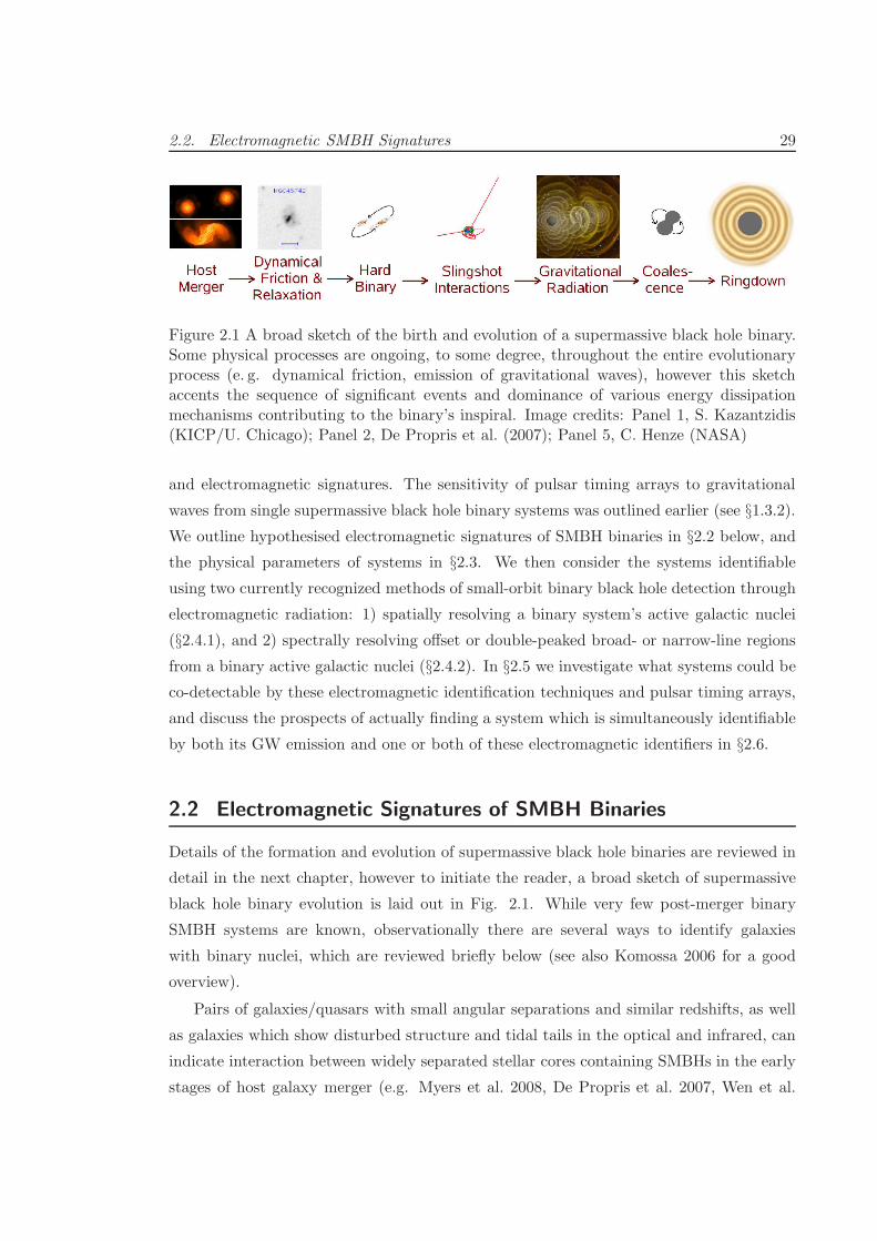
2.2. Electromagnetic SMBH Signatures 29
Figure 2.1 A broad sketch of the birth and evolution of a supermassive black hole binary.Some physical processes are ongoing, to some degree, throughout the entire evolutionaryprocess (e. g. dynamical friction, emission of gravitational waves), however this sketchaccents the sequence of significant events and dominance of various energy dissipationmechanisms contributing to the binary’s inspiral. Image credits: Panel 1, S. Kazantzidis(KICP/U. Chicago); Panel 2, De Propris et al. (2007); Panel 5, C. Henze (NASA)
and electromagnetic signatures. The sensitivity of pulsar timing arrays to gravitational
waves from single supermassive black hole binary systems was outlined earlier (see §1.3.2).We outline hypothesised electromagnetic signatures of SMBH binaries in §2.2 below, and
the physical parameters of systems in §2.3. We then consider the systems identifiable
using two currently recognized methods of small-orbit binary black hole detection through
electromagnetic radiation: 1) spatially resolving a binary system’s active galactic nuclei
(§2.4.1), and 2) spectrally resolving offset or double-peaked broad- or narrow-line regions
from a binary active galactic nuclei (§2.4.2). In §2.5 we investigate what systems could be
co-detectable by these electromagnetic identification techniques and pulsar timing arrays,
and discuss the prospects of actually finding a system which is simultaneously identifiable
by both its GW emission and one or both of these electromagnetic identifiers in §2.6.
2.2 Electromagnetic Signatures of SMBH Binaries
Details of the formation and evolution of supermassive black hole binaries are reviewed in
detail in the next chapter, however to initiate the reader, a broad sketch of supermassive
black hole binary evolution is laid out in Fig. 2.1. While very few post-merger binary
SMBH systems are known, observationally there are several ways to identify galaxies
with binary nuclei, which are reviewed briefly below (see also Komossa 2006 for a good
overview).
Pairs of galaxies/quasars with small angular separations and similar redshifts, as well
as galaxies which show disturbed structure and tidal tails in the optical and infrared, can
indicate interaction between widely separated stellar cores containing SMBHs in the early
stages of host galaxy merger (e.g. Myers et al. 2008, De Propris et al. 2007, Wen et al.
30 Chapter 2. Co-detectability of Gravitational and Electromagnetic Waves
2009). However, after sufficient relaxation of the host galaxy, pairs are difficult to identify
through electromagnetic signatures without a direct tracer (for instance, distinct emission
from an active galactic nucleus). Nevertheless, secondary signals that have been modelled
as a consequence of a close or bound binary SMBH include quasi-periodic oscillations
in flux density (OJ287, Valtonen et al. 1988), abnormal jet morphology such as helices
or X-shaped radio jets (Saripalli & Subrahmanyan 2009, Lal & Rao 2007), and spatial
oscillations of an active galactic nucleus (3C66B, Sudou et al. 2003). For the last of these,
Sudou et al. proposed orbital parameters in the range of a system we would endeavour to
discover. However, in this instance the Sudou et al. interpretation is also a good example
of the danger in using indirect signatures to search for binary black holes. Soon after the
Sudou et al. (2003) publication, Jenet et al. (2004) noted that the system could not be
a binary with the proposed orbital parameters; if it were, it should be emitting a strong
GW signal, which was distinctly absent in pulsar timing data. We reference 3C66B below
as a proxy for a system of interest.
A binary identification technique that has arisen in recent years aims to identify sources
with abnormal (i. e. double or offset) broad/narrow emission line regions, implying active
galactic nuclei (AGN) moving at high relative velocities to each other or to the host
galaxy (e. g. Peterson et al. 1987, Comerford et al. 2009, Boroson & Lauer 2009, Decarli
et al. 2010). In some of these cases, other explanations have better suited the observed
characteristics of each source (e. g. Boroson & Lauer 2009, Gaskell 2010, Chornock et al.
2010), however for some systems most other explanations can be ruled out, and estimates
of the binary system parameters support the existence of a sub-kiloparsec, supermassive
binary system.
Most promising are systems such as 3C75, which shows two jet-emitting radio AGN
cores, NGC 6240 (Komossa et al. 2003), and other spatially resolved double X-ray or radio
emitting AGN (e.g. Wang & Gao 2010), which are straightforward to identify and can
provide a direct detection of a double SMBH system. The core regions of radio-luminous
AGN have been observed to show a distinct radio continuum spectrum which typically
peaks at radio frequencies above ∼1GHz, giving core components a characteristically flat
two-point spectral index (α > −0.5, where radio flux Fν ∝ να) at GHz frequencies (e.g.
Slee et al. 1994). This feature distinguishes the region most directly associated with
the host black hole from outer features such as larger scale jets or hotspots, which show
power-law spectra generally at or steeper than α = −0.7. Taking advantage of these unique
spectral signatures of the core regions of radio-emitting AGN at high radio frequency (1
to 90GHz), it is possible to spatially resolve and identify AGN containing multiple cores
2.3. Physical Preliminaries 31
using multifrequency gigahertz spectral imaging. It is this property that has provided the
supporting evidence for the existence of the smallest-separation binary supermassive black
hole currently known, 4C +37.11 (0402+379; Rodriguez et al. 2006).
2.3 Physical Preliminaries of SMBH Binary Systems
We use the following conventions in notation: two black holes have masses m1, m2 where
q ≡ m2/m1 < 1. The reduced mass, µ, of a system is µ = m1m2/M , whereM = m1+m2.
Variables of the format Qiph refer to the value Q of ph (ph = bin for the binary orbital
quantity, and ph = gw for the quantity of the related gravitational waves) measured by i
(where i = o is observed quantity at Earth, and i = s the physical quantity in the source
rest frame). For example, a binary’s source-rest-frame orbital period is Psbin.
A binary black hole at redshift z in a Keplerian orbit will have a period observed at
Earth of Pobin = P
sbin · (1 + z), and an orbital semi-major axis of:
a =
(
Pobin
√GM
2π(1 + z)
)2/3
. (2.1)
If the redshift z of a SMBH binary’s host is known, we can estimate the observed angular
separation of two discrete objects by calculating the co-moving radial distance to the
object:
D(z) =c
H0
∫ z
0
dz′
E(z′), (2.2)
where E(z)2 = Ωm(1 + z)3 + (1 − Ωm − ΩΛ)(1 + z)2 + ΩΛ, (e. g. Peebles 1993). Here,
we assume a geometrically flat Friedmann-Robertson-Walker Universe, with Ωm = 0.27,
ΩΛ = 0.73, and the Hubble constant H0 = 72 km s−1Mpc−1. The angular diameter
distance to an object provides the observed linear-to-angular scaling at the target object:
dA =ℓ
θ=D(z)
1 + z, (2.3)
where the projected linear separation ℓ of the objects in a binary of inclination i at orbital
phase φ is ℓ = a√
(sinφ cos i)2 + (cosφ)2. Equations 2.2 and 2.3 provide us with the
observed angular separation of two such objects:
θobs = 2.062648 × 10⁸ · ℓH0(1 + z)
c
[∫ z
0
dz′
E(z′)
]−1
mas , (2.4)
where c = 2.99792 × 10⁸ ms−1 is the speed of light and ℓ is in meters. If the system is in
32 Chapter 2. Co-detectability of Gravitational and Electromagnetic Waves
a stable orbit, the observed line-of-sight relative velocity of the two objects in a binary is
given by
∆vo = ∆vs sin i cosφ =
√
GM
asin i cosφ . (2.5)
Binary systems will emit gravitational waves at a frequency fsgw = nf
sbin, where n repre-
sents the harmonic at which the emission occurs. For the circular orbits to which we limit
our analysis, n = 2; however, n increases for eccentric orbits (Enoki et al. 2004).
2.4 Capability of Electromagnetic Identification Techniques
2.4.1 Direct Imaging of Active Galactic Nuclei
The flat-spectrum emission from radio AGN that is associated with the supermassive black
hole is highly compact, and largely unresolved down to scales of tens of µas. While it was
previously noted that these cores exhibit flat spectra between 1 and 90GHz, they will peak
(and, as a consequence, be most readily detectable) at frequencies between ∼2 and 20GHz.
Radio spectral imaging requires observation at two frequencies, where ν1 < ν2, preferably
observed simultaneously or near-simultaneously to minimise scintillation and/or intrinsic
variability effects (see §3.3). The resolution of VLBI observations is typically diffraction-
limited, giving a highest observing resolution of θr = c/(Bνobs), where B is the longest
observing element spacing, and νobs is the observing frequency of the experiment. This
technique likewise requires observations with a sufficient coverage in u− v space that the
morphology of the resulting image is representative of the source. Spectral index imaging
(again, the techniques of which are discussed in detail in the next chapter) requires tapering
of u−v data to match θr of the two frequencies and allow a spectral index map to be made.
As such, the resolving power of this technique—and the limiting factor for detecting the
small-orbit systems of interest—is θr at the lower observing frequency.
For our computations, we focus on the power of Very Long Baseline Interferometry
(VLBI) and in particular the Very Long Baseline Array (VLBA) to resolve components of
AGN to high resolutions. For the VLBA, B = 8611 km, however the effective maximum
baseline depends on a target’s sky position, and decreases most significantly for sources
of declination δ ≪ 0.
2.4.2 Offset Emission Line Identifiers
There are a number of emission-line identifiers that have been put forward as evidence of
a SMBH binary (including broad lines offset from narrow-line emission, a superimposed
2.5. Co-observable Binary Systems 33
set of blue- and red-shifted emission lines in the same series, and AGN line emission with
a line-of-sight velocity offset from the host galaxy). Given that the relative velocity of
SMBHs in a pair increases as the binary system evolves—rendering multiple line systems
more readily resolved with optical spectrometers—the identification of offset line systems
associated with small-orbit binaries is not limited by observing hardware.
Instead, the limiting factor for identifying small-orbit SMBH black hole binaries through
offset-line identifiers is a physical one; for binaries within a sufficiently small orbital sepa-
ration, the broad-line-emitting regions gravitationally bound to a black hole will be tidally
disrupted by the other. As noted by Dotti et al. (2009), this occurs when the radius of
the broad line region (BLR) associated with a black hole exceeds the Roche Lobe of that
black hole; that is, rbl < R. Following the Roche Lobe radius approximation of Eggleton
(1983), we are limited to
rbl < R =a 0.49 q2/3
0.6 q2/3 + ln(1 + q1/3). (2.6)
The size of the BLR can be measured by “reverberation mapping,” which maps the time
delay, τ between changes in the continuum flux in an AGN and the changes in the intensity
of a broad emission line in the source. This allows the estimation of the BLR radius as
rbl ≤ cτ (e. g. Bentz et al. 2009). Bentz et al. note that cτ is typically on the order of one
light day (≃ 0.8 × 10⁻³ pc), however rbl in galaxies have been found up to several orders
of magnitude larger, correlated with the continuum luminosity in multiple wave-bands
(Kaspi et al. 2005). For simplicity, here we simply set as an average hard limit that the
condition R > 0.001 pc must be met to observe a source. This corresponds to a limit of
a >0.6 q2/3 + ln(1 + q1/3)
490 q2/3pc (2.7)
for the minimum orbital semi-major axis detectable through offset line-emission identifiers.
2.5 Systems Co-observable in Electromagnetic and GW Emission
Pulsar timing and electromagnetic searches for binary AGN are related in two ways.
First, as stressed in this chapter, they can provide interesting scientific results in the
co-observation of electromagnetic and GW emission from a binary supermassive system.
Second (stressed more highly in the next chapter), the discovery of binary AGN at var-
ious stages of post-merger SMBH binary inspiral can help reveal the currently unknown
timescale taken by the binary to evolve from host-merger to the gravitational-wave dom-
34 Chapter 2. Co-detectability of Gravitational and Electromagnetic Waves
inant regime observable by pulsar timing. This latter aspect is exemplified by Figure
2.2, which indicates the cabalilities of VLBI to resolve a binary radio AGN at various
stages of its inspiral. Within a ≃ 1 kpc, these stages of merger are unresolvable by other
observational techniques (except for offset-line identifiers, however for these the physical
separation between two holes is more ambiguous).
As reviewed in section 1.3.1, pulsars have a sensitivity in the gravitational wave spec-
trum to frequencies 1/Cobs < fogw < 1/T , where 1/Cobs is the observational cadence (how
frequently one’s pulsars are observed), and T is the length of the pulsar timing data set.
As implied by Eq. 2.1 and the direct connection between the observed gravitational wave
frequency and the binary orbital period, the limits of pulsar timing arrays’ GW frequency
window put bounds on the physical systems detectable by pulsar timing arrays. This is
reflected in Figure 2.3, which indicates the systems detectable by the three techniques
considered in this manuscript. For the purposes of this plot we have maximised the linear
projected separation of the SMBH binary (i. e. φ = 0, ∴ ℓ = a).
It is apparent in Figure 2.3 that there is indeed some overlap in the systems theoret-
ically detectable by these techniques, with the most significant intersection between the
systems detectable by pulsar timing and offset line techniques. Note that the BLR limit
shown in this figure is mass-independent, however will increase in a as the mass ratio q
decreases. For pulsar timing, the detectable systems at q < 1 will have smaller orbital
radii; the largest overlap area between these two techniques, therefore, lies in equal-mass
systems.
For radio imaging the co-detectable systems are fewer, limited to the most massive
end of equal-mass binary systems at low redshifts: restricted to z . 0.01 for ground-
based observations at high radio frequency, and extended to sources of redshift z . 0.1
when using observatories capable of exceptionally long baselines, such as the upcoming
space-based VSOP-2 mission2.
2.6 Practical Considerations
2.6.1 Prospects of System Co-detection
The probability that a binary AGN has orbital parameters within the bounds of, and
detectable by, the radio imaging or offset-line techniques will depend on a number of
factors. This includes the number of (line-emitting/radio) AGN in local galaxies, the rate
1VSOP, see http://www.vsop.isas.jaxa.jp/top.html2VSOP-2, due for launch in 2012; see http://www.vsop.isas.jaxa.jp/vsop2
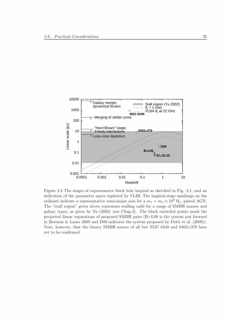
2.6. Practical Considerations 35
0.001
0.01
0.1
1
10
100
1000
10000
0.0001 0.001 0.01 0.1 1 10
Line
ar s
cale
(pc
)
Redshift
Galaxy merger;dynamical friction
Merging of stellar cores
Stall region (Yu 2002)θr = 1 masVLBA θr at 22 GHz
"Hard Binary" stage;3-body interactions
Loss-cone depletion
NGC 6240
0402+379
4C+22.25
B+L09
D09
Figure 2.2 The stages of supermassive black hole inspiral as sketched in Fig. 2.1, and anindication of the parameter space explored by VLBI. The inspiral-stage markings on theordinate indicate a representative semi-major axis for a m1 = m2 ≃ 108 M⊙ paired AGN.The “stall region” given above represents stalling radii for a range of SMBH masses andgalaxy types, as given by Yu (2002) (see Chap.3). The black encircled points mark theprojected linear separations of proposed SMBH pairs (B+L09 is the system put forwardin Boroson & Lauer 2009 and D09 indicates the system proposed by Dotti et al. (2009)).Note, however, that the binary SMBH nature of all but NGC 6240 and 0402+379 haveyet to be confirmed.
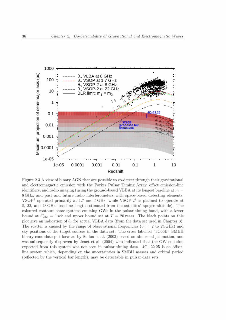
36 Chapter 2. Co-detectability of Gravitational and Electromagnetic Waves
1e-05
0.0001
0.001
0.01
0.1
1
10
100
1000
1e-05 0.0001 0.001 0.01 0.1 1 10
Max
imum
pro
ject
ion
of s
emi-m
ajor
axi
s (p
c)
Redshift
θr, VLBA at 8 GHzθr, VSOP at 1.7 GHzθr, VSOP-2 at 8 GHzθr, VSOP-2 at 22 GHzBLR limit; m1 = m2
m1,m
2=10 10M
sunm
1,m2=10 9
Msun
m1,m
2=10 8M
sunm
1,m2=10 7
Msun
m1,m
2=10 6M
sun
4C+22.25
3C66B(proposed butdebunked)
Figure 2.3 A view of binary AGN that are possible to co-detect through their gravitationaland electromagnetic emission with the Parkes Pulsar Timing Array, offset emission-lineidentifiers, and radio imaging (using the ground-based VLBA at its longest baseline at ν1 =8GHz, and past and future radio interferometers with space-based detecting elements:VSOP1 operated primarily at 1.7 and 5GHz, while VSOP-22 is planned to operate at8, 22, and 43GHz; baseline length estimated from the satellites’ apogee altitude). Thecoloured contours show systems emitting GWs in the pulsar timing band, with a lowerbound at Cobs = 1wk and upper bound set at T = 20 years. The black points on thisplot give an indication of θr for actual VLBA data (from the data set used in Chapter 3).The scatter is caused by the range of observational frequencies (v1 = 2 to 24GHz) andsky positions of the target sources in the data set. The cross labelled “3C66B” SMBHbinary candidate put forward by Sudou et al. (2003) based on abnormal jet motion, andwas subsequently disproven by Jenet et al. (2004) who indicated that the GW emissionexpected from this system was not seen in pulsar timing data. 4C+22.25 is an offset-line system which, depending on the uncertainties in SMBH masses and orbital period(reflected by the vertical bar length), may be detectable in pulsar data sets.
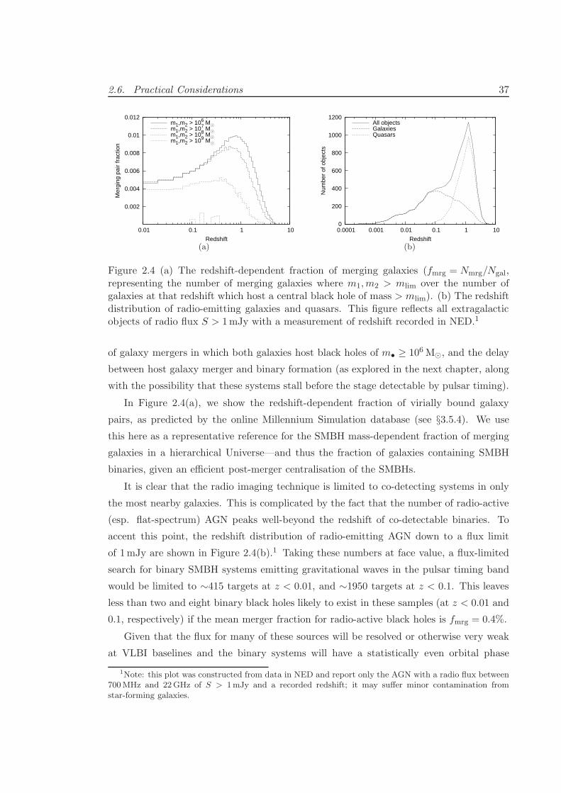
2.6. Practical Considerations 37
0.002
0.004
0.006
0.008
0.01
0.012
0.01 0.1 1 10
Mer
ging
pai
r fr
actio
n
Redshift
m1,m2 > 106 M⊙
m1,m2 > 107 M⊙
m1,m2 > 108 M⊙
m1,m2 > 109 M⊙
(a)
0
200
400
600
800
1000
1200
0.0001 0.001 0.01 0.1 1 10
Num
ber
of o
bjec
ts
Redshift
All objectsGalaxiesQuasars
(b)
Figure 2.4 (a) The redshift-dependent fraction of merging galaxies (fmrg = Nmrg/Ngal,representing the number of merging galaxies where m1,m2 > mlim over the number ofgalaxies at that redshift which host a central black hole of mass > mlim). (b) The redshiftdistribution of radio-emitting galaxies and quasars. This figure reflects all extragalacticobjects of radio flux S > 1mJy with a measurement of redshift recorded in NED.1
of galaxy mergers in which both galaxies host black holes of m• ≥ 106 M⊙, and the delay
between host galaxy merger and binary formation (as explored in the next chapter, along
with the possibility that these systems stall before the stage detectable by pulsar timing).
In Figure 2.4(a), we show the redshift-dependent fraction of virially bound galaxy
pairs, as predicted by the online Millennium Simulation database (see §3.5.4). We use
this here as a representative reference for the SMBH mass-dependent fraction of merging
galaxies in a hierarchical Universe—and thus the fraction of galaxies containing SMBH
binaries, given an efficient post-merger centralisation of the SMBHs.
It is clear that the radio imaging technique is limited to co-detecting systems in only
the most nearby galaxies. This is complicated by the fact that the number of radio-active
(esp. flat-spectrum) AGN peaks well-beyond the redshift of co-detectable binaries. To
accent this point, the redshift distribution of radio-emitting AGN down to a flux limit
of 1mJy are shown in Figure 2.4(b).1 Taking these numbers at face value, a flux-limited
search for binary SMBH systems emitting gravitational waves in the pulsar timing band
would be limited to ∼415 targets at z < 0.01, and ∼1950 targets at z < 0.1. This leaves
less than two and eight binary black holes likely to exist in these samples (at z < 0.01 and
0.1, respectively) if the mean merger fraction for radio-active black holes is fmrg = 0.4%.
Given that the flux for many of these sources will be resolved or otherwise very weak
at VLBI baselines and the binary systems will have a statistically even orbital phase
1Note: this plot was constructed from data in NED and report only the AGN with a radio flux between700MHz and 22GHz of S > 1mJy and a recorded redshift; it may suffer minor contamination fromstar-forming galaxies.
38 Chapter 2. Co-detectability of Gravitational and Electromagnetic Waves
distribution, the actual number of detectable targets will in practice be less, leaving little
prospect for success in finding a pulsar-detectable, GW-emitting system in a radio mapping
survey. However, as previously stated, and demonstrated in Chapter 3, such searches can
nevertheless contribute to measurements of the SMBH inspiral timescale.
For the offset-line technique, the lack of redshift limit to which the systems are de-
tectable and the non-constraint of radio activity allows the possibility to search of a far
greater number of objects for GW-emitting binaries; the NASA Extragalactic Database
(NED) contains over 90,000 catalogued type 1 AGN (that is, Seyfert-1 or Quasars with
detected broad-line emission). Based on the merger rates from the Millennium Database
(Springel et al. 2005; see §3.5.4) in Fig. 2.4(a), 300 to 900 of these AGN should be paired
systems. If data were acquired with enough sensitivity to search for, detect and resolve
offset lines in these sources, one would have a strong chance of multiple object detection,
even when accounting for the low line-of-sight velocity offsets that some systems will have
due to their phase and inclination orientation at the time of observation.
2.6.2 Sensitivity Considerations for Pulsar Timing
In the sections above we have considered only the frequency range of gravitational waves
explored by pulsar timing. We point out now that in fact some sources emitting in the
pulsar timing band may not be detectable because they have too small a GW strain to
induce sufficient power in pulsar timing residuals, such that it is above the noise in the
timing data set. This will have a complex dependence on the GW frequency of the binary,
the constituent masses, the binary’s distance, and the detection method of the pulsar
timing array (take, e. g., the curve of Fig. 1.5 as a reference for one pulsar).
We additionally note that although the overlap between pulsar timing and electromag-
netic identifiers increases with longer data sets, the lower-frequency binaries will likewise be
emitting fainter GW signals. Nevertheless, as timing data sets improve their RMS residual
levels and as techniques are developed for using the full power of a timing array—rather
than individual pulsars—to search for and detect GW emission, it is not inconceivable
that one or more co-detectable systems may arise in the coming decades.
2.7 Conclusions
In this chapter we have shown that three direct tracers of supermassive black hole binaries—
VLBI radio spectral imaging, multiple-peaked AGN spectral lines, and gravitational waves—
have overlap in the supermassive binary systems that they are able to detect. Radio
2.7. Conclusions 39
spectral imaging techniques are limited on small scales by the instrumental resolution
of current radio telescopes, giving this method overlap with pulsar timing’s sensitivity
to gravitational waves only at low (z . 0.1) redshift (even with the satellite-based long
baseline interferometry programs past and planned). Offset-line identification techniques,
given sufficient integration times, have no redshift-dependent detectability constraints, so
the lower limit on binary separations identifiable using this technique is placed by the
radius at which the line-emitting material is tidally stripped by the companion black hole
(this should begin to occur at orbital separations of a few milliparsec).
The chance of finding a system detectable through both its electromagnetic and gravi-
tational wave emission will depend highly on the merger rate and the distribution of AGN
in the local Universe, and the amount of time spent in a gravitational-wave-emitting state.
Using simple estimates for the merger rate and distribution of radio- and line-emitting
AGN in the Universe, we find that line-emitting systems should be more successful in
identifying these systems. The identification of co-emitting systems by resolving a double
radio core it is highly improbable, however this technique should still contribute success-
fully to identifying larger-separation binaries at an earlier stage of inspiral, contributing to
studies of galactic dynamics, merger rates, and other observable signatures of SMBH bina-
ries. The improvements in pulsar timing’s sensitivity to individual GW-emitting systems
that is expected to occur with a dedicated pulsar timing program on the upcoming Square
Kilometre Array should contribute to making the identification of co-detectable systems a
more realistic possibility, particularly if it allows a better understanding of low-frequency
timing noise over data spans of 10-20 years.

3A Radio Census of Binary Supermassive Black Holes
A non-detection is still a detection of nothing!
—G. B. Hobbs
In this chapter we carry out a search for binary supermassive black holes, further
developing the radio spectral index imaging technique noted in Chapter 2. While aiming
to detect individual systems co-observable by puslar timing arrays, we also measure the
timescale of post-merger SMBH binary inspiral, a value which was hitherto a significant
unknown, and which contributes directly to the predicted strength of the pulsar-detectable
gravitational wave background. We provide the first observational evidence against the
theoretical possibility that SMBH binaries may “stall” at ∼pc orbits—a prospect which,
if more than a theoretical fancy, would greatly impact the predictions for PTA-detectable
binary systems and the strength of the gravitational wave background.
3.1 Introduction
Models of the Universe in which hierarchical merging dominates the growth of galaxies have
strong predictions for the presence of binary supermassive black holes at galaxy centres
(e.g. Volonteri et al. 2003). As galaxies containing such massive black holes collide, the
central black holes are expected to inspiral and form a bound interacting system which will
have a significant impact on the central galactic environment (Merritt 2006). Predictions
of the strength of the astrophysical gravitational wave background from SMBH binaries,
and the expected detection rates for LISA and pulsar timing of individual black holes,
are based on parameterisations of merger rates and the SMBH population (Rajagopal
& Romani 1995, Jaffe & Backer 2003, Wyithe & Loeb 2003, Enoki et al. 2004, Sesana
et al. 2008, 2009), giving gravitational wave detectors (detailed in §1.3.1) the potential to
provide unique insights into the processes of galaxy formation.
41
42 Chapter 3. A Search for Binary Supermassive Black Holes
In theoretical treatments, however, the evolution of post-merger central supermassive
black holes still holds significant uncertainties. The steps in binary black hole formation
and evolution were first laid out by Begelman et al. (1980). After a galaxy pair becomes
virially bound, dynamical friction and violent relaxation drive the stellar cores containing
the massive black holes (of masses m1 and m2;m1 > m2) to the centre of the merger rem-
nant on roughly a dynamical friction time. When the cores have merged, the black holes
independently experience dynamical friction against the merged core’s stellar environment.
This further centralises each black hole, leading the system to become a bound pair at a
separation where the enclosed stellar mass equals the total binary mass. If the stellar core
is modelled as a single isothermal sphere with stellar density ρ∗(r) = σ2v/(2πGr2), this
occurs when the black holes reach a orbital semi-major axis of
abin =3
2
G(m1 +m2)
σ2v, (3.1)
where σv is the velocity dispersion of the merger remnant.1 The length of time spent by
black holes to reach this stage follows the Chandrasekhar timescale for dynamical friction,
and is limited by the inspiral timescale for the less massive black hole (cf. Lacey & Cole
1993):
tdf = 1.654r2σv
Gm2lnΛ, (3.2)
where we have assumed circular black hole orbits, and r is the orbital radius of the less
massive black hole from the centre of the galactic potential. In such a system, we can
assume a value for the Coulomb logarithm lnΛ ≃ 5 (a non-circular orbit with ellipticity
ǫ = 0.5 will add a factor of roughly 0.5 to the timescale and the logarithm will be 2 .
lnΛ . 3; e.g. Gualandris & Merritt 2008). The black holes will form a binary when
r = abin.
The orbital evolution of the black holes proceeds further due to dynamical friction,
however as the binary tightens and increases in velocity, dynamical friction becomes an
ineffective means of energy transfer and the rate of inspiral slows. In this intermediate
inspiral stage, there are significant uncertainties in both inspiral mechanism and timescale.
Relaxing stars in radial orbits entering the “loss cone” of the massive binary (Frank &
Rees 1976) will undergo 3-body interactions with the SMBH binary system and be ejected,
carrying away angular momentum and further shrinking the binary orbit. However, with-
out an additional mechanism for energy transfer or a means to efficiently refill the loss
cone, the binary inspiral halts as the loss cone is emptied. Recognising the long timescale
1See Sec. 3.5.2 for discussion of typical m1,m2, and σv values.
3.1. Introduction 43
that loss cone re-population might take for binary systems, Begelman et al. (1980) suggest
the possibility of gas ejection from the system or gas accretion onto the larger black hole,
which will cause shrinkage in the binary orbit to conserve angular momentum (see also,
e. g., Merritt & Milosavljevic 2005). If some intermediate process is able to sufficiently
shrink the binary orbit, gravitational radiation will cause a binary with ellipticity ǫ = 0
to coalesce in a timescale
tg =5c5
256G3
a4
m1m2(m1 +m2). (3.3)
N-body simulations and semi-analytical models have manifested various intermediate
inspiral processes (see, e.g., the extensive review of Colpi & Dotti 2009). The “last parsec
problem” is the name given to the hurdle encountered by nearly all merger models in
which the intermediate inspiral mechanisms have timescales sufficiently long that they are
unable to bring the binary to a regime in which the emission of gravitational radiation can
drive the black holes to coalescence in less than a Hubble time. If this is the case, there
may be many instances of “stalled” binary objects which spend a large portion of their
lifetimes with orbital radii within the range 0.01-10 pc (Yu 2002). A functional form for
the stalling radius is estimated by Merritt (2006):
astall2 abin
= 0.2m1/m2
(1 +m1/m2)2. (3.4)
If systems are unable to find the fuel to reach coalescence in less than the age of the
Universe, then they may appear to stall indefinitely at orbits greater (thus GW frequencies
lower, and amplitudes generally smaller) than those in the range detectable by either pulsar
timing arrays or LISA. This would have dramatic consequences for GW detectors and for
hierarchical formation models alike.
Since few small-orbit binary systems are known and electromagnetic tracers of post-
merger galaxy cores are hard to identify, it has been difficult to study the post-merger
dynamics of binary black hole systems. To date, there has been no targeted search for
small-orbit binary black holes. However, as previously noted, several recent searches for
double AGN have looked for characteristic optical/IR AGN emission lines with double-
peaks or line-of-sight velocity measurements which are offset from the host galaxy, implying
an inspiralling binary at unknown separation (Comerford et al. 2009, Boroson & Lauer
2009; e.g.). The full VLBI Imaging and Polarimetry survey (VIPS, Helmboldt et al. 2007),
has the potential for a large volume of spectral index data, and there are plans to perform
a search of similar method to the one presented in this chapter. Nevertheless, with only
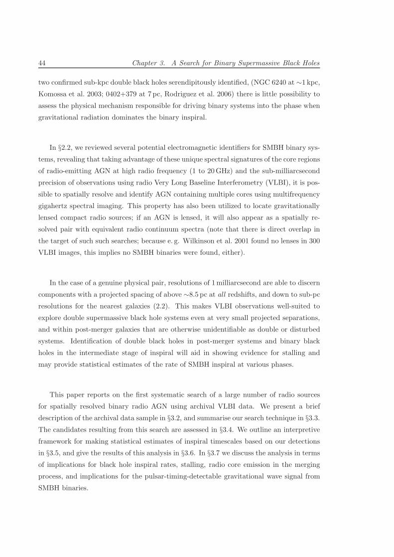
44 Chapter 3. A Search for Binary Supermassive Black Holes
two confirmed sub-kpc double black holes serendipitously identified, (NGC 6240 at ∼1 kpc,
Komossa et al. 2003; 0402+379 at 7 pc, Rodriguez et al. 2006) there is little possibility to
assess the physical mechanism responsible for driving binary systems into the phase when
gravitational radiation dominates the binary inspiral.
In §2.2, we reviewed several potential electromagnetic identifiers for SMBH binary sys-
tems, revealing that taking advantage of these unique spectral signatures of the core regions
of radio-emitting AGN at high radio frequency (1 to 20GHz) and the sub-milliarcsecond
precision of observations using radio Very Long Baseline Interferometry (VLBI), it is pos-
sible to spatially resolve and identify AGN containing multiple cores using multifrequency
gigahertz spectral imaging. This property has also been utilized to locate gravitationally
lensed compact radio sources; if an AGN is lensed, it will also appear as a spatially re-
solved pair with equivalent radio continuum spectra (note that there is direct overlap in
the target of such such searches; because e. g. Wilkinson et al. 2001 found no lenses in 300
VLBI images, this implies no SMBH binaries were found, either).
In the case of a genuine physical pair, resolutions of 1milliarcsecond are able to discern
components with a projected spacing of above ∼8.5 pc at all redshifts, and down to sub-pc
resolutions for the nearest galaxies (2.2). This makes VLBI observations well-suited to
explore double supermassive black hole systems even at very small projected separations,
and within post-merger galaxies that are otherwise unidentifiable as double or disturbed
systems. Identification of double black holes in post-merger systems and binary black
holes in the intermediate stage of inspiral will aid in showing evidence for stalling and
may provide statistical estimates of the rate of SMBH inspiral at various phases.
This paper reports on the first systematic search of a large number of radio sources
for spatially resolved binary radio AGN using archival VLBI data. We present a brief
description of the archival data sample in §3.2, and summarise our search technique in §3.3.The candidates resulting from this search are assessed in §3.4. We outline an interpretive
framework for making statistical estimates of inspiral timescales based on our detections
in §3.5, and give the results of this analysis in §3.6. In §3.7 we discuss the analysis in terms
of implications for black hole inspiral rates, stalling, radio core emission in the merging
process, and implications for the pulsar-timing-detectable gravitational wave signal from
SMBH binaries.
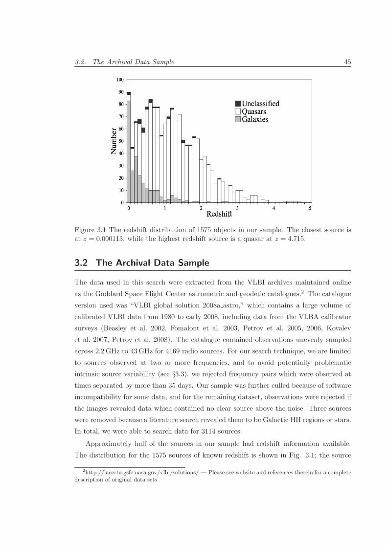
3.2. The Archival Data Sample 45
Figure 3.1 The redshift distribution of 1575 objects in our sample. The closest source isat z = 0.000113, while the highest redshift source is a quasar at z = 4.715.
3.2 The Archival Data Sample
The data used in this search were extracted from the VLBI archives maintained online
as the Goddard Space Flight Center astrometric and geodetic catalogues.2 The catalogue
version used was “VLBI global solution 2008a astro,” which contains a large volume of
calibrated VLBI data from 1980 to early 2008, including data from the VLBA calibrator
surveys (Beasley et al. 2002, Fomalont et al. 2003, Petrov et al. 2005, 2006, Kovalev
et al. 2007, Petrov et al. 2008). The catalogue contained observations unevenly sampled
across 2.2GHz to 43GHz for 4169 radio sources. For our search technique, we are limited
to sources observed at two or more frequencies, and to avoid potentially problematic
intrinsic source variability (see §3.3), we rejected frequency pairs which were observed at
times separated by more than 35 days. Our sample was further culled because of software
incompatibility for some data, and for the remaining dataset, observations were rejected if
the images revealed data which contained no clear source above the noise. Three sources
were removed because a literature search revealed them to be Galactic HII regions or stars.
In total, we were able to search data for 3114 sources.
Approximately half of the sources in our sample had redshift information available.
The distribution for the 1575 sources of known redshift is shown in Fig. 3.1; the source
2http://lacerta.gsfc.nasa.gov/vlbi/solutions/ — Please see website and references therein for a completedescription of original data sets
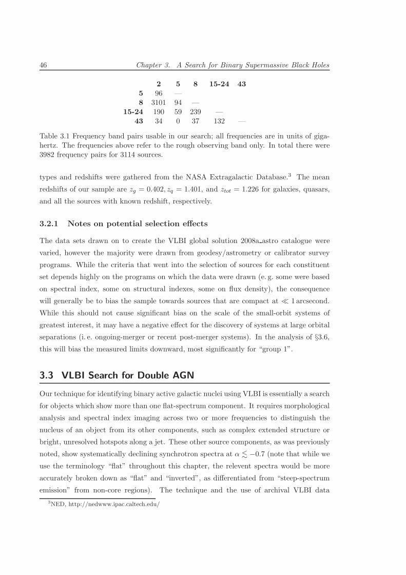
46 Chapter 3. A Search for Binary Supermassive Black Holes
2 5 8 15-24 435 96 —8 3101 94 —
15-24 190 59 239 —43 34 0 37 132 —
Table 3.1 Frequency band pairs usable in our search; all frequencies are in units of giga-hertz. The frequencies above refer to the rough observing band only. In total there were3982 frequency pairs for 3114 sources.
types and redshifts were gathered from the NASA Extragalactic Database.3 The mean
redshifts of our sample are zg = 0.402, zq = 1.401, and ztot = 1.226 for galaxies, quasars,
and all the sources with known redshift, respectively.
3.2.1 Notes on potential selection effects
The data sets drawn on to create the VLBI global solution 2008a astro catalogue were
varied, however the majority were drawn from geodesy/astrometry or calibrator survey
programs. While the criteria that went into the selection of sources for each constituent
set depends highly on the programs on which the data were drawn (e. g. some were based
on spectral index, some on structural indexes, some on flux density), the consequence
will generally be to bias the sample towards sources that are compact at ≪ 1 arcsecond.
While this should not cause significant bias on the scale of the small-orbit systems of
greatest interest, it may have a negative effect for the discovery of systems at large orbital
separations (i. e. ongoing-merger or recent post-merger systems). In the analysis of §3.6,this will bias the measured limits downward, most significantly for “group 1”.
3.3 VLBI Search for Double AGN
Our technique for identifying binary active galactic nuclei using VLBI is essentially a search
for objects which show more than one flat-spectrum component. It requires morphological
analysis and spectral index imaging across two or more frequencies to distinguish the
nucleus of an object from its other components, such as complex extended structure or
bright, unresolved hotspots along a jet. These other source components, as was previously
noted, show systematically declining synchrotron spectra at α . −0.7 (note that while we
use the terminology “flat” throughout this chapter, the relevent spectra would be more
accurately broken down as “flat” and “inverted”, as differentiated from “steep-spectrum
emission” from non-core regions). The technique and the use of archival VLBI data
3NED, http://nedwww.ipac.caltech.edu/
3.3. VLBI Search for Double AGN 47
require several precautions, primarily because both the accuracy of frequency-dependent
flux density measurements and morphological fidelity of the radio image are important to
this method.
We therefore take special precaution in considering AGN variability and coverage of
the spatial-frequency (u − v) plane for the data sets. The variability exhibited by some
radio AGN typically comes in two different flavours. Both particularly affect compact
regions of emission with high brightness temperature, such as radio cores. The first is
intra-day variability (IDV) due to propagation effects in the interstellar medium. This
signal flickering can occur on sub-day timescales and exhibits a significant modulation
index at frequencies below 5GHz, causing fluctuations on average at the 1-10% level (e.g.
Walker 1998, Lovell et al. 2008). Intrinsic variability in radio AGN cores is observed
most significantly at frequencies above 5GHz, and occurs on a wide range of timescales.
Some radio AGN exhibit slow variations on timescales of years. The existence of such
variations place limitations on the allowable temporal spacing between observations at
different frequencies. Instantaneous multifrequency spectra will not be influenced by either
effect, while observations spaced at less than the characteristic timescales of long-term
AGN variability will allay the effects of a wandering high-frequency signal. For this reason
we used only frequency pairs with a time separation of less than 35 days. Out of the 3982
usable frequency pairs in our data, 3447 were taken simultaneously, leaving 535 with an
average difference in observation time of about 11 days.
All data processing was done using the Miriad software package (Sault et al. 1995).
For each frequency pair, we inverted the u−v data, tapering the maxima of u and v to give
a circular synthesised beam of the same size at the two frequencies. A manual inspection
of u−v coverage for the pairs ensured that the sources were sampled enough to provide an
accurate representation of the source morphology at the tapered resolution. Images were
cleaned, restored with the synthesised Gaussian beam of the tapered resolution to make
images of 512x512 pixels, allowing a typical field of view 1.2 arcseconds to a side (though
varying with the resolution of the observation; this equates to a linear scale at z = 1 of
∼9.5 kpc). An estimate of the image noise level at each frequency was determined using
an off-source region of each image. The number of frequency pairs we were able to use is
detailed in Table 3.1.
The data were imaged in three ways for manual candidate searching. First, for each
resolution-matched frequency pair, the full-field-of-view images at low and high frequency
were plotted in greyscale with logarithmic contours beginning at three times the noise level
of each image. Enhanced plots of the central image regions were made in a similar fashion,
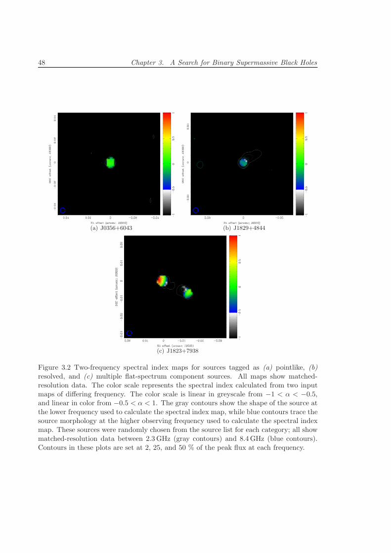
48 Chapter 3. A Search for Binary Supermassive Black Holes
(a) J0356+6043 (b) J1829+4844
(c) J1823+7938
Figure 3.2 Two-frequency spectral index maps for sources tagged as (a) pointlike, (b)resolved, and (c) multiple flat-spectrum component sources. All maps show matched-resolution data. The color scale represents the spectral index calculated from two inputmaps of differing frequency. The color scale is linear in greyscale from −1 < α < −0.5,and linear in color from −0.5 < α < 1. The gray contours show the shape of the source atthe lower frequency used to calculate the spectral index map, while blue contours trace thesource morphology at the higher observing frequency used to calculate the spectral indexmap. These sources were randomly chosen from the source list for each category; all showmatched-resolution data between 2.3GHz (gray contours) and 8.4GHz (blue contours).Contours in these plots are set at 2, 25, and 50 % of the peak flux at each frequency.
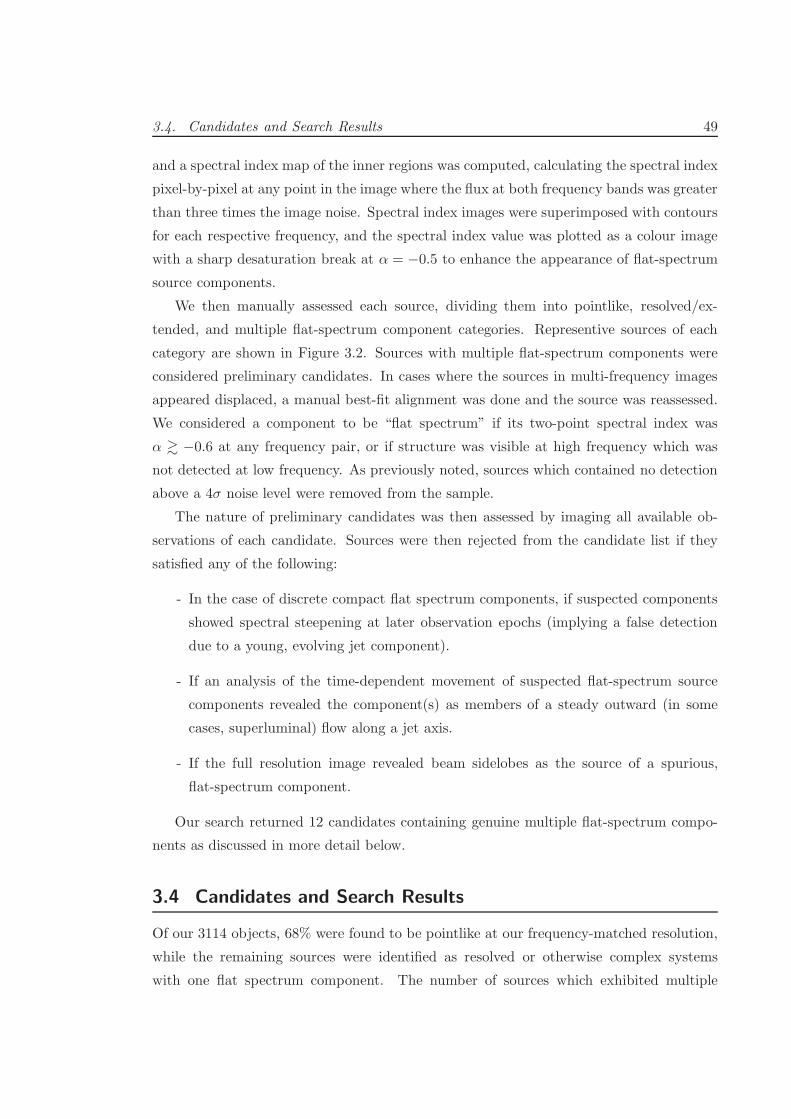
3.4. Candidates and Search Results 49
and a spectral index map of the inner regions was computed, calculating the spectral index
pixel-by-pixel at any point in the image where the flux at both frequency bands was greater
than three times the image noise. Spectral index images were superimposed with contours
for each respective frequency, and the spectral index value was plotted as a colour image
with a sharp desaturation break at α = −0.5 to enhance the appearance of flat-spectrum
source components.
We then manually assessed each source, dividing them into pointlike, resolved/ex-
tended, and multiple flat-spectrum component categories. Representive sources of each
category are shown in Figure 3.2. Sources with multiple flat-spectrum components were
considered preliminary candidates. In cases where the sources in multi-frequency images
appeared displaced, a manual best-fit alignment was done and the source was reassessed.
We considered a component to be “flat spectrum” if its two-point spectral index was
α & −0.6 at any frequency pair, or if structure was visible at high frequency which was
not detected at low frequency. As previously noted, sources which contained no detection
above a 4σ noise level were removed from the sample.
The nature of preliminary candidates was then assessed by imaging all available ob-
servations of each candidate. Sources were then rejected from the candidate list if they
satisfied any of the following:
- In the case of discrete compact flat spectrum components, if suspected components
showed spectral steepening at later observation epochs (implying a false detection
due to a young, evolving jet component).
- If an analysis of the time-dependent movement of suspected flat-spectrum source
components revealed the component(s) as members of a steady outward (in some
cases, superluminal) flow along a jet axis.
- If the full resolution image revealed beam sidelobes as the source of a spurious,
flat-spectrum component.
Our search returned 12 candidates containing genuine multiple flat-spectrum compo-
nents as discussed in more detail below.
3.4 Candidates and Search Results
Of our 3114 objects, 68% were found to be pointlike at our frequency-matched resolution,
while the remaining sources were identified as resolved or otherwise complex systems
with one flat spectrum component. The number of sources which exhibited multiple
50 Chapter 3. A Search for Binary Supermassive Black Holes
(a) Candidate J0541-0541 (b) Candidate J1658+0741
(c) Candidate J2246-1206
Figure 3.3 Example two-frequency spectral index and contour maps for three of the initialcandidates described in §3.4.1. Coloring of the mapped data and contours are as in Fig.3.2. Contours are set at 4, 16, 64, and 256 times the RMS image noise drawn from therespective frequency’s input image.
3.4. Candidates and Search Results 51
flat-spectrum components comprised less than 4 percent of the sample, and after the
assessment of preliminary candidates, there remained 12 candidate binary sources. As
an example of our candidate data quality, spectral and two-frequency contour images for
three of the candidates below are shown in Figure 3.3. One candidate was the binary
black hole candidate published by Rodriguez et al. (2006), 0402+379; an investigation of
this source is available in their publication. The remainder of our candidates appear to
contain regions with active jet injection, which effectively gives rise to a population of
contaminants for the radio spectral index mapping technique, requiring further data and
analysis to distinguish such a source from a binary black hole. Below we use our data and
that available from the literature to further investigate each source and gather evidence
for the presence of such processes, and not a binary black hole, in the sources.
Ultimately, we report the detection of no new binary systems. We have searched
a sample of considerable size, finding only one spatially resolved binary black hole out
of 3114 radio-bright AGN. Therefore, within the limitations of our search and data, we
find 0.032% of sources in our sample in which a binary radio AGN was detected. The
implications of this are discussed in later sections.
3.4.1 Candidates with Active Relativistic Injection
Eleven of twelve candidates were rejected after the examination of all available data (in
our data, the literature, or available online4) revealed that the multiple flat-spectrum
components are in a state of active injection of relativistic electrons in a collimated jet.
These sources can be discriminated from a binary SMBH by several indicators, including
proper (superluminal) motion, or by the resolving of the emission in higher resolution maps
and alignment of the components with a more extensive outflow. Jet components may
exhibit superluminal motion depending on the jet angle, and exhibit spectral steepening as
the electrons age and lose energy; it is furthermore possible that a steadily fuelled outflow
impacting on a dense plasma can maintain a flat spectral index as new relativistic electrons
are constantly introduced. In some cases, we could not dismiss candidates because we
did not have data spanning sufficient epochs to measure spectral steepening or assess
component mobility. However, there are two further indicators that distinguish these
sources from double AGN. The first is a morphological trait; by doing component modelling
of the source in the highest resolution observation, one can infer the existence of unresolved
components in the source. For flat spectrum components best fit by a Gaussian larger
4We made use of the MOJAVE database at http://www.physics.purdue.edu/MOJAVE, which is main-tained by the MOJAVE team Lister et al. (2009).
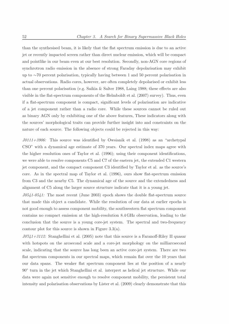
52 Chapter 3. A Search for Binary Supermassive Black Holes
than the synthesised beam, it is likely that the flat spectrum emission is due to an active
jet or recently impacted screen rather than direct nuclear emission, which will be compact
and pointlike in our beam even at our best resolution. Secondly, non-AGN core regions of
synchrotron radio emission in the absence of strong Faraday depolarisation may exhibit
up to ∼70 percent polarisation, typically having between 1 and 50 percent polarisation in
actual observations. Radio cores, however, are often completely depolarised or exhibit less
than one percent polarisation (e.g. Saikia & Salter 1988, Laing 1988; these effects are also
visible in the flat-spectrum components of the Helmboldt et al. (2007) survey). Thus, even
if a flat-spectrum component is compact, significant levels of polarisation are indicative
of a jet component rather than a radio core. While these sources cannot be ruled out
as binary AGN only by exhibiting one of the above features, These indicators along with
the sources’ morphological traits can provide further insight into and constraints on the
nature of each source. The following objects could be rejected in this way:
J0111+3906: This source was identified by Owsianik et al. (1998) as an “archetypal
CSO” with a dynamical age estimate of 370 years. Our spectral index maps agree with
the higher resolution ones of Taylor et al. (1996); using their component identifications,
we were able to resolve components C5 and C7 of the eastern jet, the extended C1 western
jet component, and the compact component C3 identified by Taylor et al. as the source’s
core. As in the spectral map of Taylor et al. (1996), ours show flat-spectrum emission
from C3 and the nearby C5. The dynamical age of the source and the extendedness and
alignment of C5 along the larger source structure indicate that it is a young jet.
J0541-0541: The most recent (June 2003) epoch shows the double flat-spectrum source
that made this object a candidate. While the resolution of our data at earlier epochs is
not good enough to assess component mobility, the southwestern flat spectrum component
contains no compact emission at the high-resolution 8.4GHz observation, leading to the
conclusion that the source is a young core-jet system. The spectral and two-frequency
contour plot for this source is shown in Figure 3.3(a).
J0741+3112: Stanghellini et al. (2005) note that this source is a Faranoff-Riley II quasar
with hotspots on the arcsecond scale and a core-jet morphology on the milliarcsecond
scale, indicating that the source has long been an active core-jet system. There are two
flat spectrum components in our spectral maps, which remain flat over the 10 years that
our data spans. The weaker flat spectrum component lies at the position of a nearly
90 turn in the jet which Stanghellini et al. interpret as helical jet structure. While our
data were again not sensitive enough to resolve component mobility, the persistent total
intensity and polarisation observations by Lister et al. (2009) clearly demonstrate that this
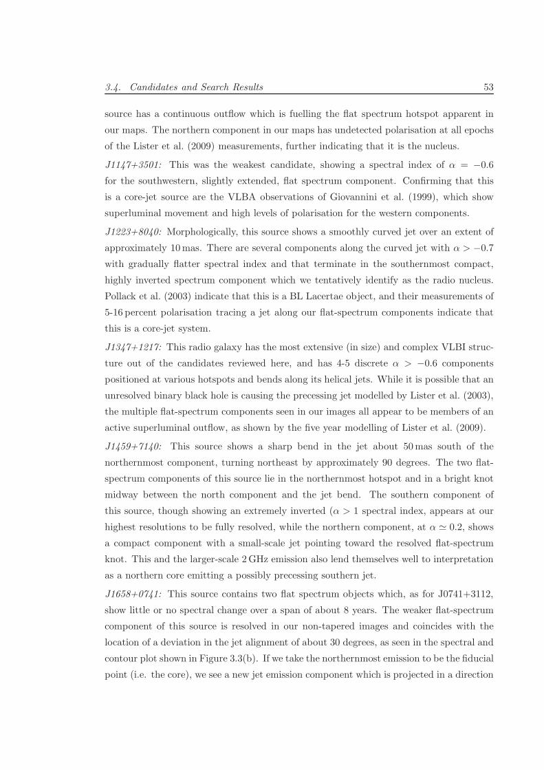
3.4. Candidates and Search Results 53
source has a continuous outflow which is fuelling the flat spectrum hotspot apparent in
our maps. The northern component in our maps has undetected polarisation at all epochs
of the Lister et al. (2009) measurements, further indicating that it is the nucleus.
J1147+3501: This was the weakest candidate, showing a spectral index of α = −0.6
for the southwestern, slightly extended, flat spectrum component. Confirming that this
is a core-jet source are the VLBA observations of Giovannini et al. (1999), which show
superluminal movement and high levels of polarisation for the western components.
J1223+8040: Morphologically, this source shows a smoothly curved jet over an extent of
approximately 10mas. There are several components along the curved jet with α > −0.7
with gradually flatter spectral index and that terminate in the southernmost compact,
highly inverted spectrum component which we tentatively identify as the radio nucleus.
Pollack et al. (2003) indicate that this is a BL Lacertae object, and their measurements of
5-16 percent polarisation tracing a jet along our flat-spectrum components indicate that
this is a core-jet system.
J1347+1217: This radio galaxy has the most extensive (in size) and complex VLBI struc-
ture out of the candidates reviewed here, and has 4-5 discrete α > −0.6 components
positioned at various hotspots and bends along its helical jets. While it is possible that an
unresolved binary black hole is causing the precessing jet modelled by Lister et al. (2003),
the multiple flat-spectrum components seen in our images all appear to be members of an
active superluminal outflow, as shown by the five year modelling of Lister et al. (2009).
J1459+7140: This source shows a sharp bend in the jet about 50mas south of the
northernmost component, turning northeast by approximately 90 degrees. The two flat-
spectrum components of this source lie in the northernmost hotspot and in a bright knot
midway between the north component and the jet bend. The southern component of
this source, though showing an extremely inverted (α > 1 spectral index, appears at our
highest resolutions to be fully resolved, while the northern component, at α ≃ 0.2, shows
a compact component with a small-scale jet pointing toward the resolved flat-spectrum
knot. This and the larger-scale 2GHz emission also lend themselves well to interpretation
as a northern core emitting a possibly precessing southern jet.
J1658+0741: This source contains two flat spectrum objects which, as for J0741+3112,
show little or no spectral change over a span of about 8 years. The weaker flat-spectrum
component of this source is resolved in our non-tapered images and coincides with the
location of a deviation in the jet alignment of about 30 degrees, as seen in the spectral and
contour plot shown in Figure 3.3(b). If we take the northernmost emission to be the fiducial
point (i.e. the core), we see a new jet emission component which is projected in a direction
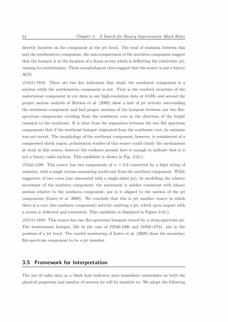
54 Chapter 3. A Search for Binary Supermassive Black Holes
directly incident on the component at the jet bend. The trail of emission between this
and the southeastern component, the non-compactness of the northern component suggest
that the hotspot is at the location of a dense screen which is deflecting the relativistic jet,
causing its reorientation. These morphological clues suggest that the source is not a binary
AGN.
J1823+7938: There are two key indicators that imply the southwest component is a
nucleus while the northeastern component is not. First is the resolved structure of the
easternmost component in our data in our high-resolution data at 8GHz and second the
proper motion analysis of Britzen et al. (2008) show a hub of jet activity surrounding
the southwest component and find proper motions of the hotspots between our two flat-
spectrum components receding from the southwest core in the direction of the bright
emission to the northeast. It is clear from the separation between the two flat spectrum
components that if the northeast hotspot originated from the southwest core, its emission
was not recent. The morphology of the northeast component, however, is reminiscent of a
compressed shock region; polarisation studies of this source could clarify the mechanisms
at work in this source, however the evidence present here is enough to indicate that it is
not a binary radio nucleus. This candidate is shown in Fig. 3.2(c).
J2246-1206: This source has two components of α > 0.3 connected by a faint string of
emission, with a single stream emanating north-east from the northern component. While
suggestive of two cores (one associated with a single-sided jet), by modelling the relative
movement of the northern component, the movement is neither consistent with binary
motion relative to the southern component, nor is it aligned to the motion of the jet
components (Lister et al. 2009). We conclude that this is yet another source in which
there is a core (the southern component) actively emitting a jet, which upon impact with
a screen is deflected and reoriented. This candidate is displayed in Figure 3.3(c).
J2253+1608: This source has two flat-spectrum hotspots traced by a steep-spectrum jet.
The westernmost hotspot, like in the case of J2246-1206 and J1658+0741, sits in the
position of a jet bend. The careful monitoring of Lister et al. (2009) show the secondary
flat-spectrum component to be a jet member.
3.5 Framework for Interpretation
The use of radio data as a black hole indicator puts immediate constraints on both the
physical properties and number of sources we will be sensitive to. We adopt the following
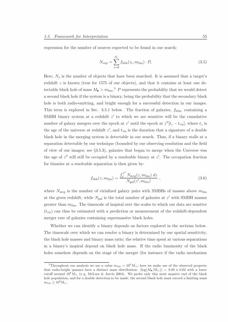
3.5. Framework for Interpretation 55
expression for the number of sources expected to be found in our search:
Nexp =
Ns∑
i=0
fbbh(zi,mlim) · Pi (3.5)
Here, Ns is the number of objects that have been searched. It is assumed that a target’s
redshift z is known (true for 1575 of our objects), and that it contains at least one de-
tectable black hole of massM• > mlim.5 P represents the probability that we would detect
a second black hole if the system is a binary, being the probability that the secondary black
hole is both radio-emitting, and bright enough for a successful detection in our images.
This term is explored in Sec. 3.5.1 below. The fraction of galaxies, fbbh, containing a
SMBH binary system at a redshift z′ to which we are sensitive will be the cumulative
number of galaxy mergers over the epoch at z′ until the epoch at z′′[tz − tvis], where tz is
the age of the universe at redshift z′, and tvis is the duration that a signature of a double
black hole in the merging system is detectable in our search. Thus, if a binary stalls at a
separation detectable by our technique (bounded by our observing resolution and the field
of view of our images; see §3.5.3), galaxies that began to merge when the Universe was
the age of z′′ will still be occupied by a resolvable binary at z′. The occupation fraction
for binaries at a resolvable separation is then given by:
fbbh(z,mlim) =
∫ z′′
z′ Nmrg(z,mlim) dz
Ngal(z′,mlim), (3.6)
where Nmrg is the number of virialized galaxy pairs with SMBHs of masses above mlim
at the given redshift, while Ngal is the total number of galaxies at z′ with SMBH masses
greater than mlim. The timescale of inspiral over the scales to which our data are senstive
(tvis) can thus be estimated with a prediction or measurement of the redshift-dependent
merger rate of galaxies containing supermassive black holes.
Whether we can identify a binary depends on factors explored in the sections below.
The timescale over which we can resolve a binary is determined by our spatial sensitivity,
the black hole masses and binary mass ratio; the relative time spent at various separations
in a binary’s inspiral depend on black hole mass. If the radio luminosity of the black
holes somehow depends on the stage of the merger (for instance if the radio mechanism
5Throughout our analysis we use a value mlim = 108 M⊙; here we make use of the observed propertythat radio-bright quasars have a distinct mass distribution: 〈log(M•/M⊙)〉 = 8.89 ± 0.02 with a lowercutoff around 108 M⊙ (e. g. McLure & Jarvis 2004). We probe only this most massive end of the blackhole population, and for a double detection to be made, the second black hole must exceed a limiting massmlim ≥ 108M⊙.
56 Chapter 3. A Search for Binary Supermassive Black Holes
shuts down as the galaxies begin interacting, or ignites only after a binary coalescence),
an additional factor needs to be considered in Eq. 3.5. However, because the evidence
for a relationship between radio fuelling and merger events has until now been tenuous
and estimates for an AGN timescale are so far inconclusive, we limit this uncertainty by
employing two scenarios below that represent the most optimistic and the most pessimistic
expectations for the state of radio luminosity in the two black holes.
3.5.1 Supermassive Black Holes and Radio Emission
All our targets are radio sources detectable on parsec scales, and it follows that all contain
at least one radio-emitting supermassive black hole. If a target is a binary system with
a resolvable separation between the two black holes, due to our inspection techniques a
second radio-emitting SMBH will have only been flagged as a candidate if its flux density
exceeds four times the root-mean-squared noise (σrms) in its image. This 4σrms flux limit
corresponds to a luminosity sensitivity limit of Llim(σrms, z). To predict the expected
number of binary AGN to be found in our search and estimate a timescale for binary
SMBH inspiral, we must first quantify the likelihood that the radio emission of a second
black hole will exceed this luminosity limit.
The main unknown contributing to the discussion is how strongly the galactic and
intergalactic environment relate to the production of radio AGN activity around the central
black hole: that is, do the merger and mixing of gaseous, dusty, and stellar environments
contribute strongly the production of radio activity? Below we assign two scenarios to
bound assumptions at either end of extremes: 1) Pessimistic; the probability that a SMBH
paired with a radio-emitting AGN is itself radio-emitting is no greater than the probability
that a non-binary SMBH at the center of a massive galaxy would be radio-emitting, and
2) Optimistic; given a black hole that exists in a shared environment with a radio-emitting
AGN, the probability of radio emission in the second black hole is unity.
Given that the black holes in the progenitors may not encounter significantly mixed
environments until the binary has a relatively small separation, it is also possible that radio
ignition is radially dependent. Regardless, we stress that for the third stage of inspiral
in which theoretically the binary may stall, the stellar cores around the black holes have
merged and the black holes will have shared many orbits within one another’s sphere of
influence and in a common environment.
3.5. Framework for Interpretation 57
Pessimistic scenario
We can make an estimate of the fewest number of binary sources we would expect to see by
setting P equal to the integrated bivariate luminosity function of galaxies, ψ(M,>Llim),
where M represents the absolute optical/infrared magnitude of a galaxy. In this case
we assume that mergers have no influence on the radio-active state of a black hole; that
is, that the probability that the second black hole in a binary would have a detectable
luminosity L > Llim is equivalent to the radio active fraction for non-merging galaxies
selected from a random pool with M• ≥ mlim. We calculate P for each source using a
log-linear interpolation of the integrated bivariate luminosity function of Mauch & Sadler
(2007) for radio AGNs in galaxies with −24 > MK ≥ −25, taking such galaxies to be
representative of our targets’ host galaxies. As roughly 10% of the Mauch & Sadler (2007)
sample have flat spectra (based on the measurements of Mason et al. (2009)), we expect
that approximately 10% of their sources will be compact down to VLBI scales. To account
for this we divide the space density given in their radio luminosity function by a factor
of 10. For our 1575 sources with a known redshift, we find that in this scenario P has a
mean and standard deviation of 0.4% and 1%, respectively.
Optimistic scenario
In the optimistic scenario, we consider that a SMBH in the presence of a radio AGN will
itself be a radio-loud AGN. This scenario implies that when the two black holes share a
common galactic environment, both black holes will be radio luminous if the conditions
are fit for radio ignition; that is, both objects will be either radio-loud or not. We take
as a given that one black hole is a detectable radio AGN in each of our images. To
determine the detectability of a second SMBH in such a system (the probability that its
observed luminosity is greater than Llim), we would like to avoid the explicit use of e. g.
relativistic beaming models, correlations between black hole mass and radio luminosity,
and the levels of flux resolved by our baselines—the parameters of which are uncertain—by
using an estimate derived from observations in which such effects are inherent.
We therefore take the secondary SMBHs in such systems to have a radio luminosity dis-
tribution equal to the luminosity distribution of solitary, flat-spectrum radio black holes,
which will implicitly include beaming and mass-correlation effects. The use of the flat-
spectrum population assumes that the emission observed in flat-spectrum radio sources is
largely unresolved, and therefore scalable to the resolutions reached by our VLBI data. We
adopt a probability density function for secondary black hole radio luminosities, ρ(z, L) dL,
based on the redshift-dependent, flat-spectrum “pure luminosity evolution model” of Dun-
58 Chapter 3. A Search for Binary Supermassive Black Holes
lop & Peacock (1990). We may then determine the probability that for a given object in
the sample, a second black hole will have a luminosity above our detection threshold, Llim.
The probability that we would have detected the second black hole of a binary AGN is
therefore:
P =1
ρn
∫ ∞
Llim
ρ(z, L) dL . (3.7)
The normalisation factor, ρn =∫∞
LRLρ(z, L) dL, sets the range of radio luminosities of
radio-loud AGN. We use a lower luminosity bound of LRL = 1023 WHz−1 sr−1 for radio
AGN, equal to that given by Padovani et al. (2009). Although the exact value of LRL
debatable, the average P value is not highly sensitive to the value of ρn if LRL is decreased.
For images in which the Llim < LRL, the probability of detection is set to one. For the
1575 known-redshift sources in this scenario, P has a mean and standard deviation of
57.9% and 23.7%, respectively.
3.5.2 Host Properties and Limiting Radii
The predicted binary formation radii and stalling radii mark key points in possible inspiral
rate changes for a post-merger system. In order to determine what stage of inspiral we have
probed with our spatial sensitivity limits, we require an estimate of the predicted typical
abin and astall for our sample. As mergers between less massive galaxies are expected
to be more common than high mass mergers, for this study we expect the least massive
(and most common) merger probed in our sample to involve two black holes of 108 M⊙.
Relevant progenitor galaxy properties can be calculated to estimate the characteristic
scales (e.g. stalling radius, binary formation radius) that our study probes. Using two
black holes of mass 108M⊙, each progenitor’s velocity dispersion, σv ∼ 187 km s−1, and
bulge mass, Mhost ∼ 6.63×10¹⁰M⊙, can be estimated by theM•−σv relation of Ferrarese
& Merritt (2000) and the M• −Mbulge relation of Haring & Rix (2004), respectively. If
the black holes do not accrete a significant fraction of their mass during inspiral, the post-
merger galaxy will contain a black hole of 2×10⁸M⊙ and an implied velocity dispersion of
σv ∼ 216 km s−1. The binary formation radius for our typical system is thus abin = 27.7 pc,
while the stalling radius is astall = 2.8 pc (equations 3.1, 3.4). In the earliest stage of
merger, the virially bound galaxy pair will have a projected separation . 7 kpc. We note
that while these radii are the characteristic values for the sources in the sample, more
massive (and less common) mergers between 109 M⊙ black holes will have larger radii by
a factor of ∼10.
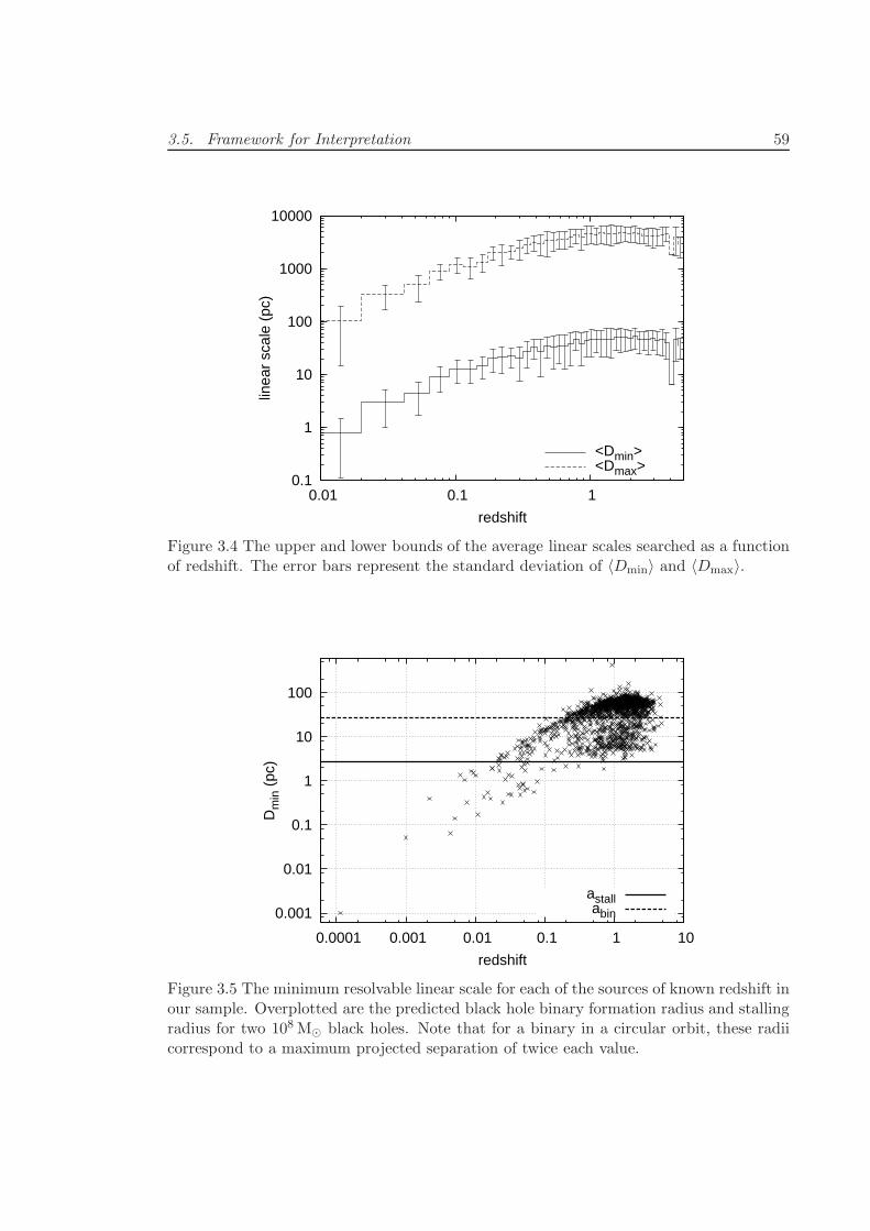
3.5. Framework for Interpretation 59
0.1
1
10
100
1000
10000
0.01 0.1 1
linea
r sc
ale
(pc)
redshift
<Dmin><Dmax>
Figure 3.4 The upper and lower bounds of the average linear scales searched as a functionof redshift. The error bars represent the standard deviation of 〈Dmin〉 and 〈Dmax〉.
0.001
0.01
0.1
1
10
100
0.0001 0.001 0.01 0.1 1 10
Dm
in (
pc)
redshift
astallabin
Figure 3.5 The minimum resolvable linear scale for each of the sources of known redshift inour sample. Overplotted are the predicted black hole binary formation radius and stallingradius for two 108 M⊙ black holes. Note that for a binary in a circular orbit, these radiicorrespond to a maximum projected separation of twice each value.
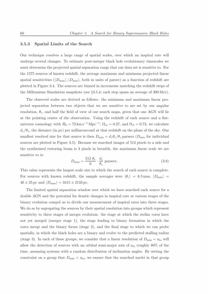
60 Chapter 3. A Search for Binary Supermassive Black Holes
3.5.3 Spatial Limits of the Search
Our technique resolves a large range of spatial scales, over which an inspiral rate will
undergo several changes. To estimate post-merger black hole evolutionary timescales we
must determine the projected spatial separation range that our data set is sensitive to. For
the 1575 sources of known redshift, the average maximum and minimum projected linear
spatial sensitivities (〈Dmax〉, 〈Dmin〉, both in units of parsec) as a function of redshift are
plotted in Figure 3.4. The sources are binned in increments matching the redshift steps of
the Millennium Simulation snapshots (see §3.5.4; each step spans an average of 300Myr).
The observed scales are derived as follows: the minimum and maximum linear pro-
jected separation between two objects that we are sensitive to are set by our angular
resolution, θr, and half the field of view of our search maps, given that one AGN will lie
at the pointing centre of the observation. Using the redshift of each source and a flat-
universe cosmology with H0 = 72 km s−1 Mpc−1, Ωm = 0.27, and ΩΛ = 0.73, we calculate
dz/θz, the distance (in pc) per milliarcsecond at that redshift on the plane of the sky. Our
smallest resolved size for that source is then Dmin = dzθr/θz parsecs (Dmin for individual
sources are plotted in Figure 3.5). Because we searched images of 512 pixels to a side and
the synthesised restoring beam is 3 pixels in breadth, the maximum linear scale we are
sensitive to is:
Dmax =512 θr
6· dzθz
parsecs . (3.8)
This value represents the largest scale size to which the search of each source is complete.
For sources with known redshift, the sample averages were 〈θr〉 = 6.5mas, 〈Dmin〉 =
40± 25 pc and 〈Dmax〉 = 3415 ± 2133 pc.
The limited spatial separation window over which we have searched each source for a
double AGN and the potential for drastic changes in inspiral rate at various stages of the
binary evolution compel us to divide our measurement of inspiral rates into three stages.
We do so by segregating the sources by their spatial resolution into groups which represent
sensitivity to three stages of merger evolution: the stage at which the stellar cores have
not yet merged (merger stage 1), the stage leading to binary formation in which the
cores merge and the binary forms (stage 2), and the final stage to which we can probe
spatially, in which the black holes are a binary and evolve to the predicted stalling radius
(stage 3). In each of these groups, we consider that a linear resolution of Dmin = alo will
allow the detection of sources with an orbital semi-major axis of alo roughly 80% of the
time, assuming systems with a random distribution of inclination angles. By setting the
constraint on a group that Dmin < alo, we ensure that the searched nuclei in that group
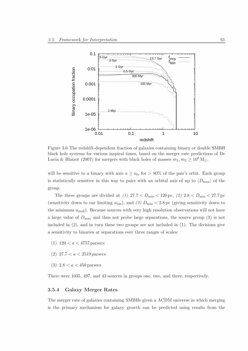
3.5. Framework for Interpretation 61
1e-06
1e-05
0.0001
0.001
0.01
0.1
0.01 0.1 1 10
Bin
ary
occu
patio
n fr
actio
n
redshift
1 Myr
100 Myr
300 Myr
0.5 Gyr1 Gyr
3 Gyr5 Gyr 13.7 Gyr fmrg
fbbh
Figure 3.6 The redshift-dependent fraction of galaxies containing binary or double SMBHblack hole systems for various inspiral times, based on the merger rate predictions of DeLucia & Blaizot (2007) for mergers with black holes of masses m1,m2 ≥ 108 M⊙.
will be sensitive to a binary with axis a ≥ alo for > 80% of the pair’s orbit. Each group
is statistically sensitive in this way to pairs with an orbital axis of up to 〈Dmax〉 of the
group.
The three groups are divided at (1) 27.7 < Dmin < 120 pc, (2) 2.8 < Dmin < 27.7 pc
(sensitivity down to our limiting abin), and (3) Dmin < 2.8 pc (giving sensitivity down to
the minimum astall). Because sources with very high resolution observations will not have
a large value of Dmax and thus not probe large separations, the source group (3) is not
included in (2), and in turn these two groups are not included in (1). The divisions give
a sensitivity to binaries at separations over three ranges of scales:
(1) 120 < a < 4757 parsecs
(2) 27.7 < a < 2519 parsecs
(3) 2.8 < a < 450 parsecs
There were 1035, 497, and 43 sources in groups one, two, and three, respectively.
3.5.4 Galaxy Merger Rates
The merger rate of galaxies containing SMBHs given a ΛCDM universe in which merging
is the primary mechanism for galaxy growth can be predicted using results from the
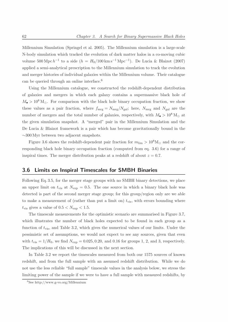
62 Chapter 3. A Search for Binary Supermassive Black Holes
Millennium Simulation (Springel et al. 2005). The Millennium simulation is a large-scale
N-body simulation which tracked the evolution of dark matter halos in a co-moving cubic
volume 500Mpch−1 to a side (h = H0/100 km s−1Mpc−1). De Lucia & Blaizot (2007)
applied a semi-analytical prescription to the Millennium simulation to track the evolution
and merger histories of individual galaxies within the Millennium volume. Their catalogue
can be queried through an online interface.6
Using the Millennium catalogue, we constructed the redshift-dependent distribution
of galaxies and mergers in which each galaxy contains a supermassive black hole of
M• > 108 M⊙. For comparison with the black hole binary occupation fraction, we show
these values as a pair fraction, where fmrg = Nmrg/Ngal; here, Nmrg and Ngal are the
number of mergers and the total number of galaxies, respectively, with M• > 108 M⊙ at
the given simulation snapshot. A “merged” pair in the Millennium Simulation and the
De Lucia & Blaizot framework is a pair which has become gravitationally bound in the
∼300Myr between two adjacent snapshots.
Figure 3.6 shows the redshift-dependent pair fraction for mlim > 108M⊙ and the cor-
responding black hole binary occupation fraction (computed from eq. 3.6) for a range of
inspiral times. The merger distribution peaks at a redshift of about z = 0.7.
3.6 Limits on Inspiral Timescales for SMBH Binaries
Following Eq. 3.5, for the merger stage groups with no SMBH binary detections, we place
an upper limit on tvis at Nexp = 0.5. The one source in which a binary black hole was
detected is part of the second merger stage group; for this group/region only are we able
to make a measurement of (rather than put a limit on) tvis, with errors bounding where
tvis gives a value of 0.5 < Nexp < 1.5.
The timescale measurements for the optimistic scenario are summarised in Figure 3.7,
which illustrates the number of black holes expected to be found in each group as a
function of tvis, and Table 3.2, which gives the numerical values of our limits. Under the
pessimistic set of assumptions, we would not expect to see any sources, given that even
with tvis = 1/H0, we find Nexp = 0.025, 0.20, and 0.16 for groups 1, 2, and 3, respectively.
The implications of this will be discussed in the next section.
In Table 3.2 we report the timescales measured from both our 1575 sources of known
redshift, and from the full sample with an assumed redshift distribution. While we do
not use the less reliable “full sample” timescale values in the analysis below, we stress the
limiting power of the sample if we were to have a full sample with measured redshifts, by
6See http://www.g-vo.org/Millennium
3.7. Discussion 63
0
2
4
6
8
10
12
100 101 102 103 104 105
Nex
p
tvis (Myr)
1/H0
stalling radius (3)
Initial inspiral (1)Merging core region (2)Bound binary + beyond
Figure 3.7 The cumulative expected number of sources and limits on the inspiral timescalefor each spatial-sensitivity limited group using the optimistic scenario (§3.5.1) in whichgiven one radio-active black hole in a binary, the second will also be radio-emitting. Forgroups 1 and 2, the upper limit set on tvis is marked with an arrow, while for group twothe measured value of tvis is marked by a filled circle, with open circles indicating the errorrange.
assuming the remaining sources have a redshift distribution equivalent to the other 1575.
This has the effect of roughly doubling Nexp for each group, and as such works only to lay
more stringent limits on tvis.
Finally, although the number of sources in group one was the largest, these sources
also had a tendency to be of higher redshift, with a net effect of fewer expected detectable
binary black holes due to the lower merging fraction of SMBH hosts at redshifts z & 1. For
stalling studies, the observation of low-redshift sources is therefore doubly beneficial: not
only does it allow smaller scales to be resolved in the sources due to their proximity, but it
affords a higher predicted success rate due to the increased merger rate of SMBH-hosting
galaxies at low redshift.
3.7 Discussion
The question we aim to answer with this search is whether there is observational evidence
for stalled supermassive binary black hole systems: that is, what is the evolution timescale
down to the stalling radius for a post-merger supermassive black hole pair? For our
methods, this question is intertwined with how closely correlated the radio emission is
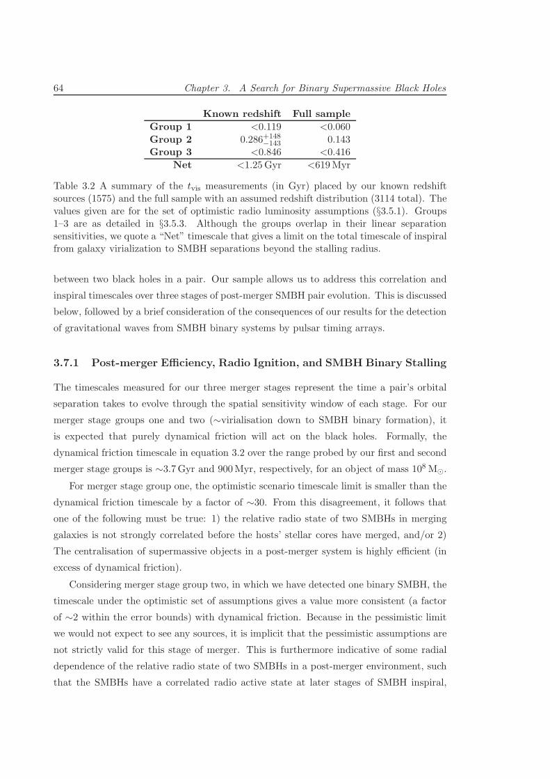
64 Chapter 3. A Search for Binary Supermassive Black Holes
Known redshift Full sample
Group 1 <0.119 <0.060
Group 2 0.286+148−143 0.143
Group 3 <0.846 <0.416
Net <1.25Gyr <619Myr
Table 3.2 A summary of the tvis measurements (in Gyr) placed by our known redshiftsources (1575) and the full sample with an assumed redshift distribution (3114 total). Thevalues given are for the set of optimistic radio luminosity assumptions (§3.5.1). Groups1–3 are as detailed in §3.5.3. Although the groups overlap in their linear separationsensitivities, we quote a “Net” timescale that gives a limit on the total timescale of inspiralfrom galaxy virialization to SMBH separations beyond the stalling radius.
between two black holes in a pair. Our sample allows us to address this correlation and
inspiral timescales over three stages of post-merger SMBH pair evolution. This is discussed
below, followed by a brief consideration of the consequences of our results for the detection
of gravitational waves from SMBH binary systems by pulsar timing arrays.
3.7.1 Post-merger Efficiency, Radio Ignition, and SMBH Binary Stalling
The timescales measured for our three merger stages represent the time a pair’s orbital
separation takes to evolve through the spatial sensitivity window of each stage. For our
merger stage groups one and two (∼virialisation down to SMBH binary formation), it
is expected that purely dynamical friction will act on the black holes. Formally, the
dynamical friction timescale in equation 3.2 over the range probed by our first and second
merger stage groups is ∼3.7Gyr and 900Myr, respectively, for an object of mass 108 M⊙.
For merger stage group one, the optimistic scenario timescale limit is smaller than the
dynamical friction timescale by a factor of ∼30. From this disagreement, it follows that
one of the following must be true: 1) the relative radio state of two SMBHs in merging
galaxies is not strongly correlated before the hosts’ stellar cores have merged, and/or 2)
The centralisation of supermassive objects in a post-merger system is highly efficient (in
excess of dynamical friction).
Considering merger stage group two, in which we have detected one binary SMBH, the
timescale under the optimistic set of assumptions gives a value more consistent (a factor
of ∼2 within the error bounds) with dynamical friction. Because in the pessimistic limit
we would not expect to see any sources, it is implicit that the pessimistic assumptions are
not strictly valid for this stage of merger. This is furthermore indicative of some radial
dependence of the relative radio state of two SMBHs in a post-merger environment, such
that the SMBHs have a correlated radio active state at later stages of SMBH inspiral,
3.7. Discussion 65
after the pair has shared a common galactic environment for many orbits.
We have set the cutoff for the third merger stage group to be sensitive to the theoretical
stalling radius of Merritt (2006). While the limits that we can place on this stage of merger
are the least stringent due to the small source count in the limiting group, they represent
the first observational exploration of stalling. If the evidence exhibited by merger stage
group 2 holds—that the relative radio state between two black holes is more strongly cor-
related at late stages of binary evolution—our results are in agreement with a progression
through the stalling radius in much less than a Hubble time; that is, we find no evidence
for systematic stalling of supermassive binary black hole systems. These results, however,
exist with the significant caveat: if the most pessimistic assumptions are true, we would
not expect to see any paired SMBHs regardless of the length of post-merger inspiral.
As previously noted and reflected in table 2, we have only used the information from
roughly half of our sources to acquire timescale measurements. The lack of detections in
the additional 1539 sources suggests that the measured limits will only be more stringent,
however would be highly dependent on the redshift distribution of the remaining sources.
3.7.2 Consequences for the GW Background and Pulsar Timing Arrays
The measured inspiral timescales and lack of evidence for stalled supermassive systems
are pertinent results for pulsar timing arrays. While we have primarily accentuated that
the brevity of inspiral timescale implies an efficient passage through the stalling stage,
we note also that the timescales measured for merger group two (in concert with time
spent at other separations) are sufficiently large that they may have non-negligible effects
on predictions of the gravitational wave background signature in the local Universe from
SMBH binaries. The GWB prediction models discussed in §1.3.1 typically assume efficient
or instantaneous inspiral into the gravitational wave regime, equating redshift-dependent
galaxy merger rates with binary coalescence rates. The inspiral times measured here
may cause the galaxies merging at a redshift of 0.7, at which the merger distribution
peaks, to emit gravitational radiation at a much later epoch, causing a larger expected
amplitude for the astrophysical gravitational wave background than previously estimated
(recall equations 1.11, 1.12). In addition, it is likely that this effect would cause an increase
in the predicted number of supermassive binary sources whose gravitational radiation is
strong enough to be resolved from the gravitational wave background by pulsar timing
arrays (Sesana et al. 2009).
66 Chapter 3. A Search for Binary Supermassive Black Holes
3.8 Summary
We have performed a search of 3114 active galactic nuclei for the presence of double SMBH
systems using a multi-frequency radio imaging technique. Of the sources searched, only
0402+379 was apparent with our method as a binary AGN. While this source has already
been put forward as a binary black hole in Rodriguez et al. (2006), this search represents
a significant enough statistical sample with which to interpret the existence of this source
in the broader cosmological context of binary supermassive black holes.
This search has probed estimates of the inspiral timescale for binary black holes of
m1,m2 ≥ 108 M⊙. For the 1575 sources that had redshift information with which to
discern the linear scales probed in the host galaxy, we obtained timescale estimates for
the inspiral of binary systems in three ranges of binary separation. We have demonstrated
observational evidence against stalled binary black hole systems by demonstrating that: 1)
at late stages of SMBH pair inspiral, the two black holes are more likely to be in a similarly
radio-active state, and 2) SMBH binaries proceed from separations of a ≃ 500 parsecs
to within the stalling radius estimates of Merritt (2006) in less than ∼0.5Gyr. The
implications of this are that supermassive binary systems do not stall indefinitely at such
radii, suggesting there is a yet undetermined mechanism by which the black holes are able
to dispense energy to the surrounding environment and proceed to coalescence.
The results of this study come with the caveat that they stem on very small-number
statistics; that is, we detected only one binary AGN in the analysis, and due to unmeasured
redshifts, we were unable to use roughly half of the sources searched in the statistical
analysis. Definitive studies of this type for large numbers of AGN would become possible
with the large collecting area and dense instantaneous u−v coverage of the planned Square
Kilometer Array (SKA). However, as implied by Eq. 2.4 and the analysis of Chapter 2, the
SKA will only be a productive research instrument for this method if long baselines are
included in its configuration (e. g. baseline length B & 1200 km at 5GHz would give the
capability of resolving the stalling regions of the most massive supermassive black hole
pairs at z < 0.01).
4An Archival Search for Radio Transients:
Implications for RRATs and Extreme Pulsar
Intermittence
The two prime movers in the Universe are Time and Luck.
—K. Vonnegut Jr.
In this chapter we develop a single pulse search methodology which makes novel ad-
ditions to the search processes reviewed in §1.4.2. We then explore the nature of RRATs
through fourteen new discoveries of sparsely-emitting neutron stars in a blind search for
transient radio bursts of between 0.125 and 32 millisecond duration. The new detections
provide key insights into RRATs and extreme nulling phenomena in pulsars, and support
the premise that RRATs may simply be nulling pulsars that are only “on” for less than a
pulse period. The newly discovered object PSR J0941–39 may futhermore represent a di-
rect link between pulsars and RRATs, as it appears to oscillate between a sparsely-emitting
“RRAT” state and a ∼10% nulling-fraction “pulsar” state.
4.1 Introduction
As reviewed in §1.4.2, the transient radio sky has revealed many classes of exotic objects
since the discovery of pulsars in late 1967 (Hewish et al. 1968), with the recent discovery
of sparsely bursting rotating radio transients (RRATs, McLaughlin et al. 2006), and a
one-off burst tentatively identified as having an extragalactic origin (Lorimer et al. 2007)
spurring renewed interest in the search for single-pulse emission after 30 years of Fourier
transform searches dominating surveys for pulsars.
67
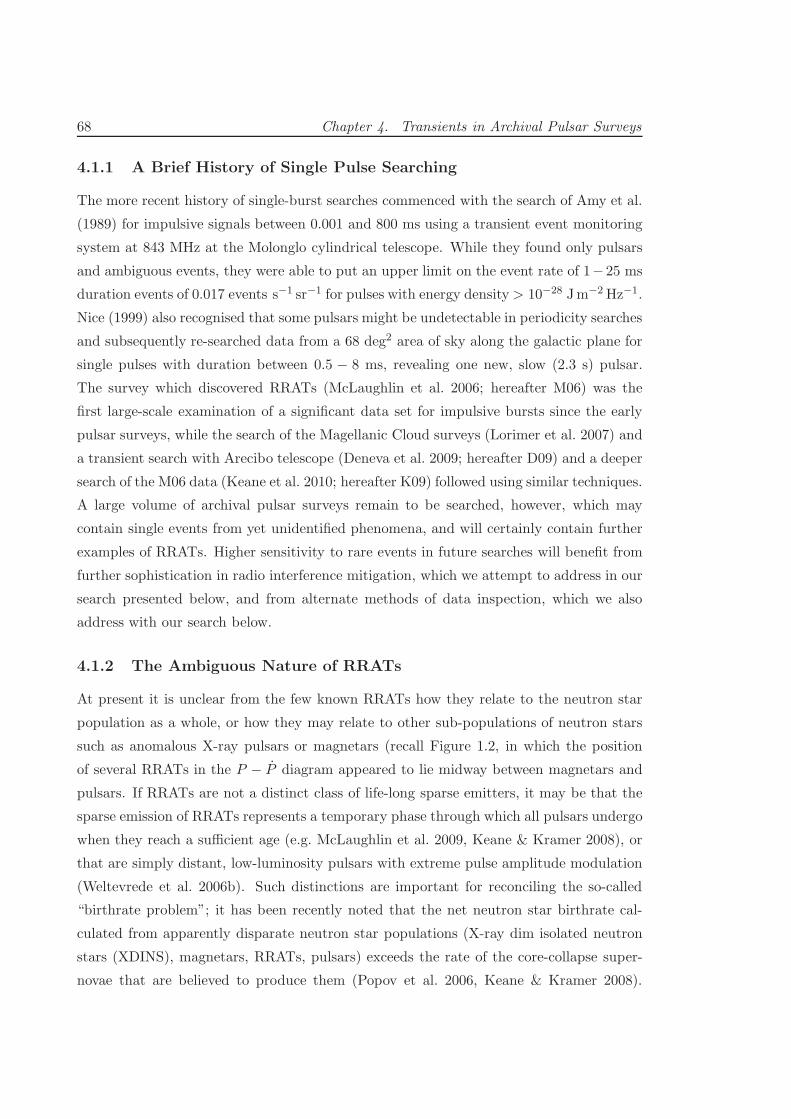
68 Chapter 4. Transients in Archival Pulsar Surveys
4.1.1 A Brief History of Single Pulse Searching
The more recent history of single-burst searches commenced with the search of Amy et al.
(1989) for impulsive signals between 0.001 and 800 ms using a transient event monitoring
system at 843 MHz at the Molonglo cylindrical telescope. While they found only pulsars
and ambiguous events, they were able to put an upper limit on the event rate of 1−25 ms
duration events of 0.017 events s−1 sr−1 for pulses with energy density> 10−28 Jm−2Hz−1.
Nice (1999) also recognised that some pulsars might be undetectable in periodicity searches
and subsequently re-searched data from a 68 deg2 area of sky along the galactic plane for
single pulses with duration between 0.5 − 8 ms, revealing one new, slow (2.3 s) pulsar.
The survey which discovered RRATs (McLaughlin et al. 2006; hereafter M06) was the
first large-scale examination of a significant data set for impulsive bursts since the early
pulsar surveys, while the search of the Magellanic Cloud surveys (Lorimer et al. 2007) and
a transient search with Arecibo telescope (Deneva et al. 2009; hereafter D09) and a deeper
search of the M06 data (Keane et al. 2010; hereafter K09) followed using similar techniques.
A large volume of archival pulsar surveys remain to be searched, however, which may
contain single events from yet unidentified phenomena, and will certainly contain further
examples of RRATs. Higher sensitivity to rare events in future searches will benefit from
further sophistication in radio interference mitigation, which we attempt to address in our
search presented below, and from alternate methods of data inspection, which we also
address with our search below.
4.1.2 The Ambiguous Nature of RRATs
At present it is unclear from the few known RRATs how they relate to the neutron star
population as a whole, or how they may relate to other sub-populations of neutron stars
such as anomalous X-ray pulsars or magnetars (recall Figure 1.2, in which the position
of several RRATs in the P − P diagram appeared to lie midway between magnetars and
pulsars. If RRATs are not a distinct class of life-long sparse emitters, it may be that the
sparse emission of RRATs represents a temporary phase through which all pulsars undergo
when they reach a sufficient age (e.g. McLaughlin et al. 2009, Keane & Kramer 2008), or
that are simply distant, low-luminosity pulsars with extreme pulse amplitude modulation
(Weltevrede et al. 2006b). Such distinctions are important for reconciling the so-called
“birthrate problem”; it has been recently noted that the net neutron star birthrate cal-
culated from apparently disparate neutron star populations (X-ray dim isolated neutron
stars (XDINS), magnetars, RRATs, pulsars) exceeds the rate of the core-collapse super-
novae that are believed to produce them (Popov et al. 2006, Keane & Kramer 2008).
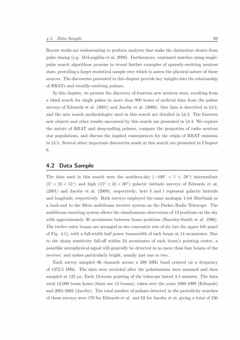
4.2. Data Sample 69
Recent works are endeavouring to perform analyses that make the distinction clearer from
pulse timing (e.g. McLaughlin et al. 2009). Furthermore, continued searches using single-
pulse search algorithms promise to reveal further examples of sparsely-emitting neutron
stars, providing a larger statistical sample over which to assess the physical nature of these
sources. The discoveries presented in this chapter provide key insights into the relationship
of RRATs and steadily-emitting pulsars.
In this chapter, we present the discovery of fourteen new neutron stars, resulting from
a blind search for single pulses in more than 900 hours of archival data from the pulsar
surveys of Edwards et al. (2001) and Jacoby et al. (2009). Our data is described in §4.2,and the new search methodologies used in this search are detailed in §4.3. The fourteen
new objects and other results uncovered by this search are presented in §4.4. We explore
the nature of RRAT and deep-nulling pulsars, compare the properties of radio neutron
star populations, and discuss the implied consequences for the origin of RRAT emission
in §4.5. Several other important discoveries made in this search are presented in Chapter
6.
4.2 Data Sample
The data used in this search were the southern-sky (−100 < l < 50) intermediate
(5 < |b| < 15) and high (15 < |b| < 30) galactic latitude surveys of Edwards et al.
(2001) and Jacoby et al. (2009), respectively; here b and l represent galactic latitude
and longitude, respectively. Both surveys employed the same analogue 1-bit filterbank as
a back-end to the 20cm multibeam receiver system on the Parkes Radio Telescope. The
multibeam receiving system allows the simultaneous observation of 13 positions on the sky
with approximately 30 arcminutes between beam positions (Staveley-Smith et al. 1996).
The twelve outer beams are arranged in two concentric sets of six (see the upper left panel
of Fig. 4.1), with a full-width half power beamwidth of each beam at 14 arcminutes. Due
to the sharp sensitivity fall-off within 24 arcminutes of each beam’s pointing centre, a
pointlike astrophysical signal will generally be detected in no more than four beams of the
receiver, and unless particularly bright, usually just one or two.
Each survey sampled 96 channels across a 288 MHz band centred on a frequency
of 1372.5 MHz. The data were recorded after the polarisations were summed and then
sampled at 125 µs. Each 13-beam pointing of the telescope lasted 4.4 minutes. The data
total 12,090 beam hours (there are 13 beams), taken over the years 1998-1999 (Edwards)
and 2001-2002 (Jacoby). The total number of pulsars detected in the periodicity searches
of these surveys were 170 for Edwards et al. and 62 for Jacoby et al, giving a total of 230
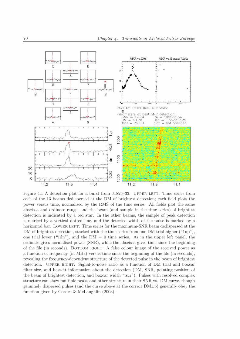
70 Chapter 4. Transients in Archival Pulsar Surveys
Figure 4.1 A detection plot for a burst from J1825–33. Upper left: Time series fromeach of the 13 beams dedispersed at the DM of brightest detection; each field plots thepower versus time, normalised by the RMS of the time series. All fields plot the sameabscissa and ordinate range, and the beam (and sample in the time series) of brightestdetection is indicated by a red star. In the other beams, the sample of peak detectionis marked by a vertical dotted line, and the detected width of the pulse is marked by ahorizontal bar. Lower left: Time series for the maximum-SNR beam dedispersed at theDM of brightest detection, stacked with the time series from one DM trial higher (“1up”),one trial lower (“1dn”), and the DM = 0 time series. As in the upper left panel, theordinate gives normalised power (SNR), while the abscissa gives time since the beginningof the file (in seconds). Bottom right: A false colour image of the received power asa function of frequency (in MHz) versus time since the beginning of the file (in seconds),revealing the frequency-dependent structure of the detected pulse in the beam of brightestdetection. Upper right: Signal-to-noise ratio as a function of DM trial and boxcarfilter size, and best-fit information about the detection (DM, SNR, pointing position ofthe beam of brightest detection, and boxcar width “tscr”). Pulses with resolved complexstructure can show multiple peaks and other structure in their SNR vs. DM curve, thoughgenuinely dispersed pulses (and the curve above at the correct DM±5) generally obey thefunction given by Cordes & McLaughlin (2003).
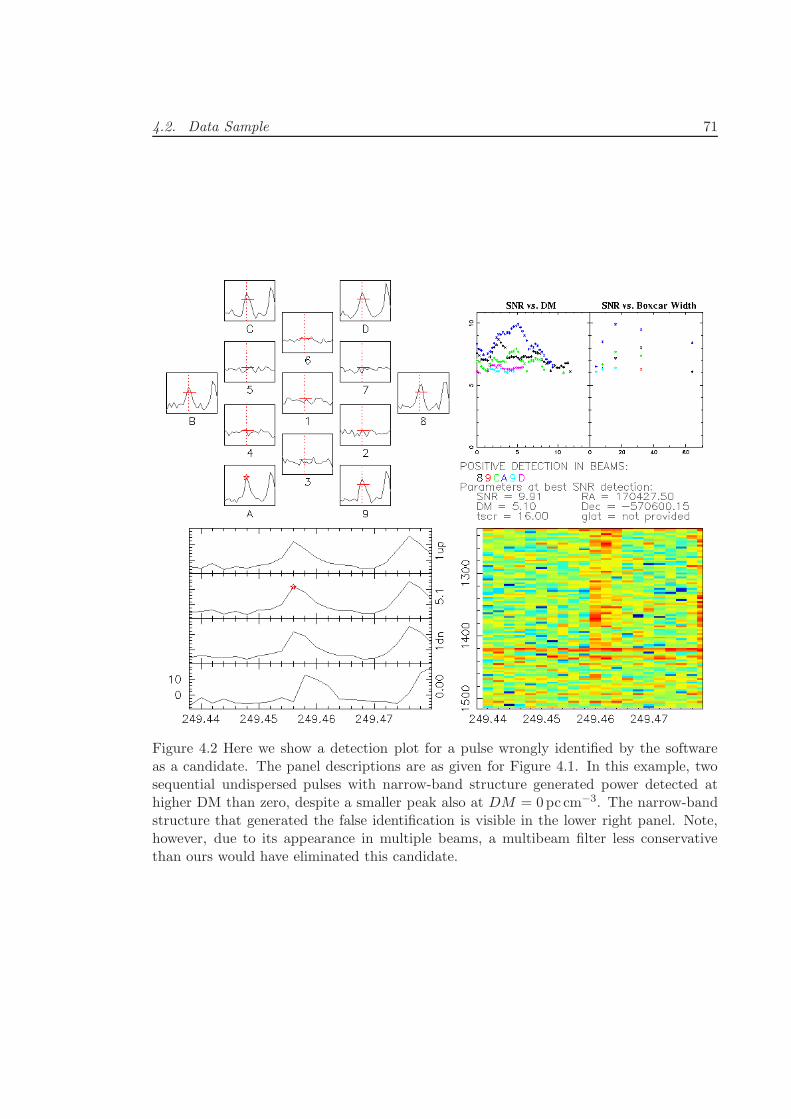
4.2. Data Sample 71
Figure 4.2 Here we show a detection plot for a pulse wrongly identified by the softwareas a candidate. The panel descriptions are as given for Figure 4.1. In this example, twosequential undispersed pulses with narrow-band structure generated power detected athigher DM than zero, despite a smaller peak also at DM = 0pc cm−3. The narrow-bandstructure that generated the false identification is visible in the lower right panel. Note,however, due to its appearance in multiple beams, a multibeam filter less conservativethan ours would have eliminated this candidate.
72 Chapter 4. Transients in Archival Pulsar Surveys
independently detected pulsars.
All follow-up data presented here were taken with the new 2-bit digital filterbank
system currently installed at Parkes Radio Telescope that use CASPER tools and is known
as BPSR. Data with this system were taken with 1024 channels across 400 MHz centred
at 1381.8 MHz, and sampled at 64 µs. Filters blocking emission from a geosynchronous
satellite visible by the telescope render frequencies above 1520 MHz unusable.
4.3 Single Burst Search Process
The most significant difficulty in single pulse searches is allaying the millions of spurious
candidates which arise from local man-made and natural radio frequency interference, such
as lightning. Our search employs various stages of automatic radio frequency interference
(RFI) elimination before candidates are manually assessed. We generally followed the steps
of Cordes & McLaughlin (2003), however with adjustments in the techniques used for RFI
rejection, matched filtering, and visual inspection. The main discriminant used in single
pulse searches is the fact that astrophysical transients exhibit a well-defined frequency-
dependent delay caused by the propagation through multiple ionised plasma screens in
the interstellar medium, visible as a time lag across the bandwidth of our instrument.
The dispersion measure, DM, measures the integrated line-of-sight column density of free
electrons in units of pc cm−3. Locally generated signals generally do not appear dispersed
(DM ∼ 0), while genuine bursts have a decrease in measured significance as the trial
dispersion increases from the true dispersion of the source. Periodic sources will show
multiple detections at the same dispersion measure. The radio interference “forest” local
to any given astronomical observing site gives rise to the need for a set of thresholds
that remove broad, zero-dispersion signals. We therefore have increased confidence in
candidates at higher dispersion.
Our detection thresholds were estimated by manual inspection of the data and trial
runs on a sub-sample of data to characterise the typical local RFI environment of the
Parkes Telescope. These tests indicated that events separated by at least 3.75 ms (30 data
bins at the native time resolution) could be considered independent, that signals peaking in
signal-to-noise ratio (SNR) below DM = 5 were most likely RFI or statistically insignficant,
and that setting a search threshold at six times the RMS noise of the dedispersed time
series was sufficient to filter out the majority of candidates which were due to statistical
fluctuations or narrow band interference.
The search process followed several steps. At each trial DM, after dedispersion the
frequency channels were summed and a search for SNR≥ 6 pulses was performed of the
4.3. Single Burst Search Process 73
complete 4.4 minute observation. An increased sensitivity search for broader pulses was
then performed, using a progressive box-car smoothing function ranging 21, 22, ..., 28 time
samples, corresponding to a maximum filter width of 32 ms. The 32ms maximum width
was chosen to significantly decrease the ratio of local to astrophysical candidates (as de-
termined by tests on a data subset), and to preserve our sensitivity to impulses of low
dispersion measure (the total delay in milliseconds across our band is roughly equivolent
in value to the dispersion measure of an impulse in units of pc cm−3). We have decreased
sensitivity to pulses of half-maximum width, w, outside the range 0.125 < w < 32 ms.
Additionally, the one-bit nature of the data made it difficult to discover pulses with width
less than a sample period, as we only had ≤ 96 functioning one-bit channels, and an RMS
that meant it was difficult to have much confidence before summing samples. We searched
in DM from 0 < DM < 600 pc cm−3, which for the galactic latitudes of the survey is
sufficient to probe out to at least 50 kpc except in the regions a few tenths of a degree
from l = 0, |b| = 5.
For each beam, a first-pass RFI rejection was performed by doing temporal coinci-
dence matching for all trial dispersions and matched filter steps; in this way we were able
to reconstruct multi-plane information about singly-detected events. A further tempo-
ral coincidence search of all remaining events was done in the 13 beams, conservatively
rejecting all candidates which had detections coincident in more than nine. After this
step, we have a full event archive in which are encoded the widest duration statistics for
detected beams, and information about the beam, DM, and smoothing filter of strongest
detection. Event archives which contained less than three events, and those which had a
peak in signal-to-noise at less than DM = 5, were rejected. This step significantly reduced
the number of high dispersion candidates which were due purely to narrow-band RFI and
small number statistics. The information in the remaining event archives were used to
make the plots used in manual candidate assessment.
The manual candidate ranking involved the viewing of each candidate using the tool
displayed in Figures 4.1 and 4.2. The panels contain information with which one can
quickly discriminate a true burst (e. g. Fig. 4.1) from a false detection (e. g. Fig. 4.2). Dur-
ing candidate viewing, we simultaneously queried the ATNF pulsar catalogue for pulsars
within two degrees of the brightest beam, such that we were able to easily determine DM
and position incidence, and attribute detections to previously known pulsars. Non-RFI
detections not associated with known pulsars were considered new transient candidates.
Assuming that detections which show repeated pulsations are part of the neutron
star population, we fit a rotation period to each object which has emitted at least three
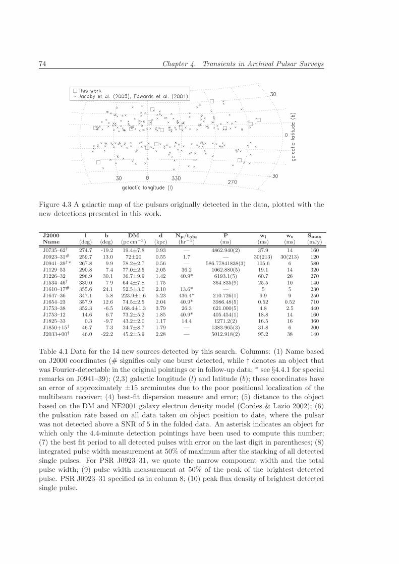
74 Chapter 4. Transients in Archival Pulsar Surveys
Figure 4.3 A galactic map of the pulsars originally detected in the data, plotted with thenew detections presented in this work.
J2000 l b DM d Np/tobs P wi ws Smax
Name (deg) (deg) (pc cm−3) (kpc) (hr−1) (ms) (ms) (ms) (mJy)
J0735–62† 274.7 -19.2 19.4±7.8 0.93 — 4862.940(2) 37.9 14 160J0923–31# 259.7 13.0 72±20 0.55 1.7 — 30(213) 30(213) 120J0941–39†* 267.8 9.9 78.2±2.7 0.56 — 586.77841838(3) 105.6 6 580J1129–53 290.8 7.4 77.0±2.5 2.05 36.2 1062.880(5) 19.1 14 320J1226–32 296.9 30.1 36.7±9.9 1.42 40.9* 6193.1(5) 60.7 26 270J1534–46† 330.0 7.9 64.4±7.8 1.75 — 364.835(9) 25.5 10 140J1610–17# 355.6 24.1 52.5±3.0 2.10 13.6* — 5 5 230J1647–36 347.1 5.8 223.9±1.6 5.23 436.4* 210.726(1) 9.9 9 250J1654–23 357.9 12.6 74.5±2.5 2.04 40.9* 3986.48(5) 0.52 0.52 710J1753–38 352.3 -6.5 168.4±1.3 3.79 26.3 621.000(5) 4.8 2.5 440J1753–12 14.6 6.7 73.2±5.2 1.85 40.9* 405.454(1) 18.8 14 160J1825–33 0.3 -9.7 43.2±2.0 1.17 14.4 1271.2(2) 16.5 16 360J1850+15† 46.7 7.3 24.7±8.7 1.79 — 1383.965(3) 31.8 6 200J2033+00† 46.0 -22.2 45.2±5.9 2.28 — 5012.918(2) 95.2 38 140
Table 4.1 Data for the 14 new sources detected by this search. Columns: (1) Name basedon J2000 coordinates (# signifies only one burst detected, while † denotes an object thatwas Fourier-detectable in the original pointings or in follow-up data; * see §4.4.1 for specialremarks on J0941–39); (2,3) galactic longitude (l) and latitude (b); these coordinates havean error of approximately ±15 arcminutes due to the poor positional localization of themultibeam receiver; (4) best-fit dispersion measure and error; (5) distance to the objectbased on the DM and NE2001 galaxy electron density model (Cordes & Lazio 2002); (6)the pulsation rate based on all data taken on object position to date, where the pulsarwas not detected above a SNR of 5 in the folded data. An asterisk indicates an object forwhich only the 4.4-minute detection pointings have been used to compute this number;(7) the best fit period to all detected pulses with error on the last digit in parentheses; (8)integrated pulse width measurement at 50% of maximum after the stacking of all detectedsingle pulses. For PSR J0923–31, we quote the narrow component width and the totalpulse width; (9) pulse width measurement at 50% of the peak of the brightest detectedpulse. PSR J0923–31 specified as in column 8; (10) peak flux density of brightest detectedsingle pulse.
4.4. Results 75
detectable pulses. Pulse periods were derived by first fitting periodicities by eye to the
detected pulses. The data were then broken into sub-integrations at the estimated period,
and sub-integrations containing on-pulses were extracted and used to do an optimised
automatic search in period and DM space using the pdmp program distributed with the
freely-available PSRchive software suite1. Where follow-up data was available and the
observations were of higher SNR, those data were used to compute the fits.
4.4 Results
Our blind search yielded the detection of several thousand single pulses with which we
could associate 91 pulsars, that were already previously detected through Fourier trans-
form search techniques by Edwards et al. (2001) and Jacoby et al. (2009), indicating that
roughly 40% of the pulsars detected in their periodicity searches have one or more de-
tectable pulses per 4.4 minute pointing. The pulsars we detected do not appear to have
any selective distribution in age or magnetic field strength, have periods ranging 0.089 to
8.5 seconds, and appear to have primarily populated the “island” of standard pulsars in
the period-period derivative diagram with periods between ∼0.1 and 3 seconds.
The new objects detected in this search include two sources which emitted only one
(albeit very convincing) pulse over the time we have observed them, and 12 sources from
which multiple pulses were observed. All of these new sources are interpreted to be errat-
ically emitting neutron stars. The best-fit parameterisations for each source are presented
in Table 4.1, and a more detailed description for each is given below. The implications of
the new detections are discussed in §4.5.
4.4.1 New Transient Sources
The properties of the pulsed sources presented here give no indication that they are
associated with a non-neutron star origin. Below we describe the properties unique
to each new object, and note the amount of follow-up time which has been dedicated
to each. Where emission was detectable in a Fourier search, the intermittency ratio
(r = SNRSinglepulse/(SNR)Fourier, as given by D09) is provided. Note that after the de-
termination of the DM from the brightest automatically-detected pulses, a manual in-
spection was done to identify weaker pulses (typically down to ∼4 times the timeseries
noise). In cases where further pulses were detected, the weaker pulses were included in
the determination of the objects’ periods and event rates.
1Available from the web on http://psrchive.sourceforge.net/
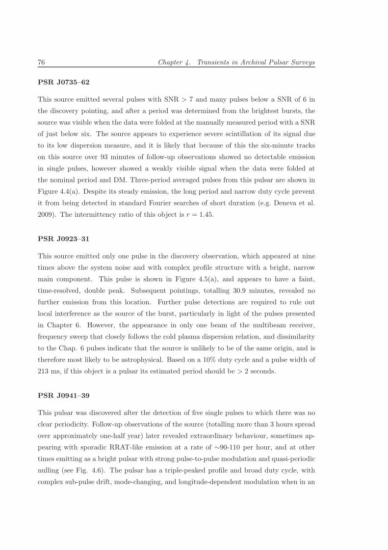
76 Chapter 4. Transients in Archival Pulsar Surveys
PSR J0735–62
This source emitted several pulses with SNR > 7 and many pulses below a SNR of 6 in
the discovery pointing, and after a period was determined from the brightest bursts, the
source was visible when the data were folded at the manually measured period with a SNR
of just below six. The source appears to experience severe scintillation of its signal due
to its low dispersion measure, and it is likely that because of this the six-minute tracks
on this source over 93 minutes of follow-up observations showed no detectable emission
in single pulses, however showed a weakly visible signal when the data were folded at
the nominal period and DM. Three-period averaged pulses from this pulsar are shown in
Figure 4.4(a). Despite its steady emission, the long period and narrow duty cycle prevent
it from being detected in standard Fourier searches of short duration (e.g. Deneva et al.
2009). The intermittency ratio of this object is r = 1.45.
PSR J0923–31
This source emitted only one pulse in the discovery observation, which appeared at nine
times above the system noise and with complex profile structure with a bright, narrow
main component. This pulse is shown in Figure 4.5(a), and appears to have a faint,
time-resolved, double peak. Subsequent pointings, totalling 30.9 minutes, revealed no
further emission from this location. Further pulse detections are required to rule out
local interference as the source of the burst, particularly in light of the pulses presented
in Chapter 6. However, the appearance in only one beam of the multibeam receiver,
frequency sweep that closely follows the cold plasma dispersion relation, and dissimilarity
to the Chap. 6 pulses indicate that the source is unlikely to be of the same origin, and is
therefore most likely to be astrophysical. Based on a 10% duty cycle and a pulse width of
213 ms, if this object is a pulsar its estimated period should be > 2 seconds.
PSR J0941–39
This pulsar was discovered after the detection of five single pulses to which there was no
clear periodicity. Follow-up observations of the source (totalling more than 3 hours spread
over approximately one-half year) later revealed extraordinary behaviour, sometimes ap-
pearing with sporadic RRAT-like emission at a rate of ∼90-110 per hour, and at other
times emitting as a bright pulsar with strong pulse-to-pulse modulation and quasi-periodic
nulling (see Fig. 4.6). The pulsar has a triple-peaked profile and broad duty cycle, with
complex sub-pulse drift, mode-changing, and longitude-dependent modulation when in an
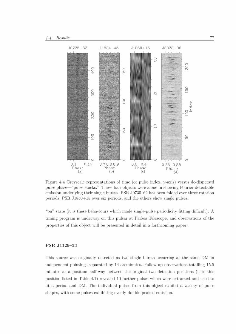
4.4. Results 77
(a) (b) (c) (d)
Figure 4.4 Greyscale representations of time (or pulse index, y-axis) versus de-dispersedpulse phase—“pulse stacks.” These four objects were alone in showing Fourier-detectableemission underlying their single bursts. PSR J0735–62 has been folded over three rotationperiods, PSR J1850+15 over six periods, and the others show single pulses.
“on” state (it is these behaviours which made single-pulse periodicity fitting difficult). A
timing program is underway on this pulsar at Parkes Telescope, and observations of the
properties of this object will be presented in detail in a forthcoming paper.
PSR J1129–53
This source was originally detected as two single bursts occurring at the same DM in
independent pointings separated by 14 arcminutes. Follow-up observations totalling 15.5
minutes at a position half-way between the original two detection positions (it is this
position listed in Table 4.1) revealed 10 further pulses which were extracted and used to
fit a period and DM. The individual pulses from this object exhibit a variety of pulse
shapes, with some pulses exhibiting evenly double-peaked emission.
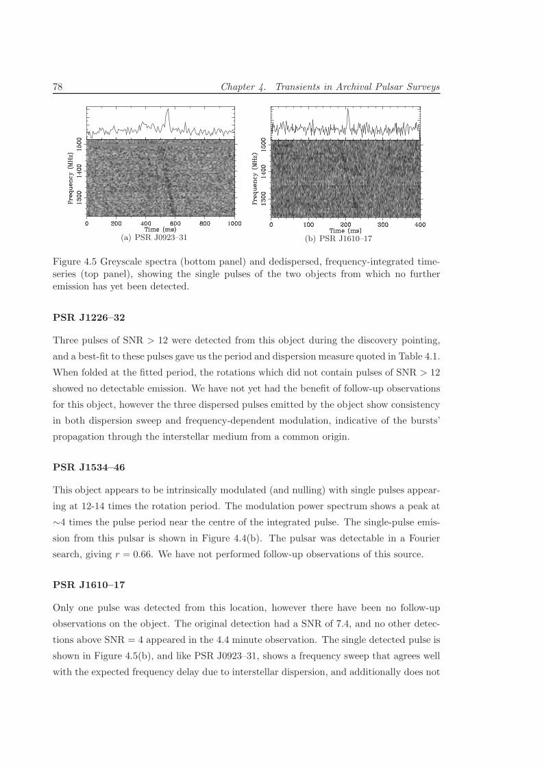
78 Chapter 4. Transients in Archival Pulsar Surveys
(a) PSR J0923–31 (b) PSR J1610–17
Figure 4.5 Greyscale spectra (bottom panel) and dedispersed, frequency-integrated time-series (top panel), showing the single pulses of the two objects from which no furtheremission has yet been detected.
PSR J1226–32
Three pulses of SNR > 12 were detected from this object during the discovery pointing,
and a best-fit to these pulses gave us the period and dispersion measure quoted in Table 4.1.
When folded at the fitted period, the rotations which did not contain pulses of SNR > 12
showed no detectable emission. We have not yet had the benefit of follow-up observations
for this object, however the three dispersed pulses emitted by the object show consistency
in both dispersion sweep and frequency-dependent modulation, indicative of the bursts’
propagation through the interstellar medium from a common origin.
PSR J1534–46
This object appears to be intrinsically modulated (and nulling) with single pulses appear-
ing at 12-14 times the rotation period. The modulation power spectrum shows a peak at
∼4 times the pulse period near the centre of the integrated pulse. The single-pulse emis-
sion from this pulsar is shown in Figure 4.4(b). The pulsar was detectable in a Fourier
search, giving r = 0.66. We have not performed follow-up observations of this source.
PSR J1610–17
Only one pulse was detected from this location, however there have been no follow-up
observations on the object. The original detection had a SNR of 7.4, and no other detec-
tions above SNR = 4 appeared in the 4.4 minute observation. The single detected pulse is
shown in Figure 4.5(b), and like PSR J0923–31, shows a frequency sweep that agrees well
with the expected frequency delay due to interstellar dispersion, and additionally does not
4.4. Results 79
Figure 4.6 Two-minute (205 rotation) pulse stacks exhibiting PSR J0941–39’s “RRAT”(off) and “Pulsar” (on) phases (§4.4.1, 4.5.3). The integrated profile shape is shown inthe panel the the right. Tracks of the signal-to-noise ratio of the peak of each pulse withSNR > 3 are plotted below the pulse stacks. The brightest peaks of the on- and off-phasesare comparable, indicating that the “off” state is not due to interstellar scintillation.
80 Chapter 4. Transients in Archival Pulsar Surveys
share the distinct properties of the Chapter 6 pulses. We suggest that although follow-up
is warranted, this pulse is likely to be of astrophysical, galactic origin.
PSR J1647–36
This pulsar appears to exhibit periodic nulling with bursts lasting on the order of 1-6 pulse
periods spaced by nulls lasting ∼27 seconds (130 rotations). With each period of “on”
activity, the bursts arrive at a phase offset by 5− 10% from the previous burst episode; it
is possible that the system is either strongly drifting or mode-changing, however follow-up
observations of this source are necessary to assess these hypotheses.
PSR J1654–23
The original detection showed 3 narrow (sub-0.5 ms), faint (SNR < 7) bursts which allowed
the fit reported in Table 4.1. The duty cycle is the smallest observed to date for a pulsar,
however due to the narrow pulses and weak emission it is possible that some pulses were
not visible above the noise. It is possible that the period reported for this pulsar could
easily be an integer multiple of the true period, the effect of which would be to broaden
the duty cycle by the same integer value. Follow-up observations of longer duration than
the discovery pointing and at a faster sampling rate will reveal more completely the nature
of this pulsar.
PSR J1753–38
The period and DM for this object were derived by extracting and fitting just the three
bright pulses detected in the original pointing. Follow-up pointings (totalling 21 minutes)
revealed further pulses consistent with the flux, period, and DM of the original detections.
PSR J1753–12
The discovery pointing containing this object was badly affected by interference. This
and the fact that only one very strong impulse was present made genuine pulse extraction
difficult, however three dispersed pulses from the object were identified and parameters
estimated. We have not yet made follow-up observations of this source, however cleaner
data may reveal more frequent low-level emission.
4.5. Discussion 81
PSR J1825–33
In the discovery pointing, this pulsar emitted seven bright, sequential pulses near the
beginning of the observation but was not visible thereafter, nor was any emission visible
in 25 minutes of follow-up observations. The profile structure of this pulsar has a double
peak (Figure 4.1 shows one pulse from this object).
PSR J1850+15
This pulsar’s discovery pointing contained strong periodic interference which probably
prevented its detection in the original Fourier search (r = 1.04; interference is visible
atop the fainter pulses of the object in Fig. 4.4(c)). The emission appears to be steady,
with no evidence for clear intermittent behaviour, although there is strong pulse-to-pulse
amplitude modulation. We have not performed follow-up observations of this source.
PSR J2033+00
This source appears to be an intermittent pulsar with a high nulling fraction and is some-
times detectable in the Fourier domain. There is some evidence of sub-pulse drift; indi-
vidual pulses rarely come from the same phase for more than a few rotations (see Figure
4.4(d)). The source was detectable in single pulses for the entirety of the 25 minute follow-
up on the source, however became distinctly brighter (and weakly detectable in a Fourier
search; r = 1.86) in the final 14 minutes.
4.5 Discussion
4.5.1 Pulsar Transient Varieties and the Nature of RRAT Emission
Regular pulsars are themselves intermittent radio sources, showing detectable emission
only for the fraction of time that their beams sweep Earth. The individual pulses, however,
are observed to show intrinsic pulse-to-pulse flux and shape differences, the origin of which
is yet unknown (though various theories exist). The variations observed in pulsars can be
broken down into two main types, being: pulse-to-pulse modulation, in which the object
emits continuously, however at an intrinsically modulated amplitude, and nulling, during
which the pulsar beam is somehow quenched, emitting no detectable radiation for a period
of time. In many pulsars, nulling appears to be a real phenomenon (with no underlying
emission when in null states), with nulls observed to occur from zero to 95% of a pulsar’s
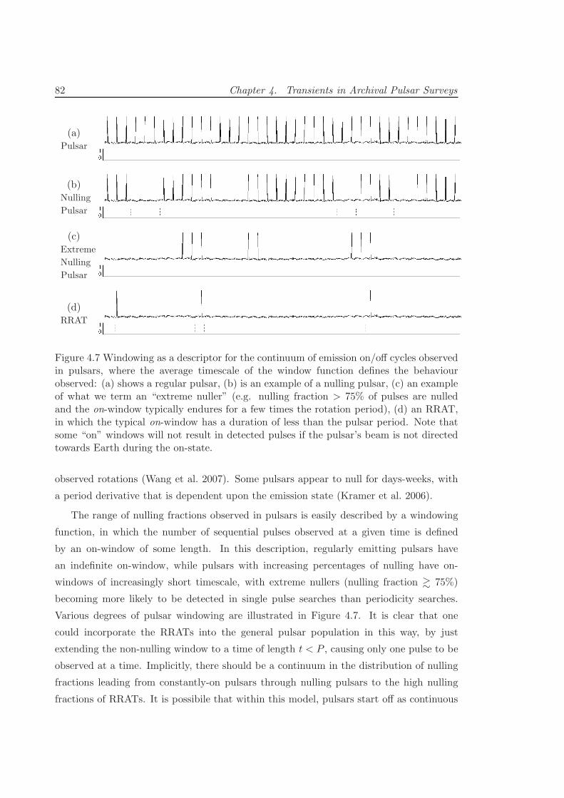
82 Chapter 4. Transients in Archival Pulsar Surveys
(a)Pulsar
(b)Nulling
Pulsar
(c)Extreme
Nulling
Pulsar
(d)RRAT
Figure 4.7 Windowing as a descriptor for the continuum of emission on/off cycles observedin pulsars, where the average timescale of the window function defines the behaviourobserved: (a) shows a regular pulsar, (b) is an example of a nulling pulsar, (c) an exampleof what we term an “extreme nuller” (e.g. nulling fraction > 75% of pulses are nulledand the on-window typically endures for a few times the rotation period), (d) an RRAT,in which the typical on-window has a duration of less than the pulsar period. Note thatsome “on” windows will not result in detected pulses if the pulsar’s beam is not directedtowards Earth during the on-state.
observed rotations (Wang et al. 2007). Some pulsars appear to null for days-weeks, with
a period derivative that is dependent upon the emission state (Kramer et al. 2006).
The range of nulling fractions observed in pulsars is easily described by a windowing
function, in which the number of sequential pulses observed at a given time is defined
by an on-window of some length. In this description, regularly emitting pulsars have
an indefinite on-window, while pulsars with increasing percentages of nulling have on-
windows of increasingly short timescale, with extreme nullers (nulling fraction & 75%)
becoming more likely to be detected in single pulse searches than periodicity searches.
Various degrees of pulsar windowing are illustrated in Figure 4.7. It is clear that one
could incorporate the RRATs into the general pulsar population in this way, by just
extending the non-nulling window to a time of length t < P , causing only one pulse to be
observed at a time. Implicitly, there should be a continuum in the distribution of nulling
fractions leading from constantly-on pulsars through nulling pulsars to the high nulling
fractions of RRATs. It is possibile that within this model, pulsars start off as continuous
4.5. Discussion 83
emitters, and gradually increase their nulling fraction until they become RRATs, which
ultimately evolve further to emit no radio emission.
The alternative view of RRAT emission, related to pulse-to-pulse modulation, was
suggested byWeltevrede et al. (2006b), who indicated that if PSR B0656+14 were observed
at several times its distance from Earth, the highly variable single pulses (emitting at up
to 420 times the average pulse flux) could emulate the single pulse behaviour observed
by M06’s distant discoveries. The pulse-energy-distribution analysis of K09, however,
makes an argument against this hypothesis (although the analysis was not done on “classic
RRATs” as we define them below). It appears obvious that there will ultimately be some
fraction of RRATs that belong to this class, but deep integrations would be expected to
show underlying emission; the real issue, therefore, is in what fraction of RRATs belong
to this class, and if some do not, what are the properties of those sources that do not?
Whether an effect of modulation or nulling, the current competing theories of RRAT
emission can be broken into three possibilities, in which the RRATs represent:
(1) a distinct class (intrinsic life-long single-pulsing)
(2) faint pulsars with extreme pulse-to-pulse modulation
(3) an evolutionary phase of pulsars, e.g. where the magnetic field degrades or the spin
period increases, leading to increased nulling fractions
Scenarios (1) and (3) intertwine similarly with questions about pulsars observed to null
(relating to whether nulling is an inherent phase of all pulsars or an effect of the local pulsar
environment). The clarification of RRATs’ nature not only has innate value, but the three
scenarios above have quite different implications for how the RRAT birthrate integrates
into that of pulsars, and how they contribute to the imbalance of core-collapse super-
nova rates and neutron star birthrates noted by Keane & Kramer (2008). For instance,
in scenario (1) the latent RRAT population may actually exceed the pulsar population.
Scenarios (2) and (3), on the other hand, are in part solutions to the birthrate problem, in
that the birthrates contributed by RRATs are effectively absorbed into those of pulsars. If
RRATs are simply distant, highly modulated pulsars, the sources detected as RRATs are
simply abnormalities among the distant, otherwise undetectable pulsars sitting below the
average luminosity limit of periodicity surveys; these distant and low-luminosity pulsars
are accounted for in pulsar birthrate analyses (e.g. Lorimer et al. 1993) with statistical
estimates, using luminosity-dependent scaling factors.
Although the original RRATs of M06 have a number of apparent properties which set
them apart from regular pulsars, as detailed in Sec. 4.5.3, we define the classic RRAT
84 Chapter 4. Transients in Archival Pulsar Surveys
as an object which emits only non-sequential single bursts with no otherwise detectable
emission at the rotation period. When using the term nulling pulsar, we refer to an object
which emits for some fraction of its rotations, however the emission coming in bursts of
several sequential pulses. Finally, we refer to all objects which emit pulses for less than
∼25% of their rotations as extreme pulsar transients.
Below we discuss the properties of our new transients and compare them with the
RRATs of M06 and with the properties of the general pulsar population.
4.5.2 A Breakdown of Our Discoveries
What is immediately striking about the 14 objects detected in this search is the variety of
dormancy timescales, covering a broad range of the nulling and modulation phenomena
related above. For some objects, such as PSR J1850+15, the lack of previous detection by
Fourier search techniques can be explained by the presence in the data of intense periodic
RFI, which lowers sensitivity to fainter periodic sources. The pulsars PSR J0735–62 and
PSR J1850+15 appear to simply be regular pulsars which were likely missed in previous
searches due to the modulation and long period of PSR J0735–62, and the presence of
interference in the discovery pointing of PSR J1850+15.
The “classic RRATs” in our search include PSRs J1129–53, J1226–32, J1654–23,
J1753–38, and J1753–12. We also place the objects from which only one pulse was ob-
served in this category; although we have not detected further events from the sources,
the pulse widths are typical of pulsars and the pulsation rates implied by our observa-
tions are consistent with the range of pulsation rates observed in the RRATs published by
M06, which ranged from one per four minutes to one per three hours. We note that the
bright single pulses emitted by PSRs J1226–32 and J1753–38 are too bright and have a
pulsation rate too high to represent a long tail of a log-normal pulse energy distribution,
immediately indicating that scenario (2) above (extreme modulation) is not the case for
all RRATs. This is less clear in the case of PSR J1753–12, and we note that our sources
may represent a mix of highly modulated low-luminosity pulsars, and true RRATs.
Apart from PSR J0941–39, the remaining objects appear to be nulling pulsars with
high nulling fractions. Only two of these objects were in an “on” state for a sufficient
fraction of observing time to be Fourier-detectable. Additionally, it is difficult to say
whether the source PSR J1825–33 is truly a nulling pulsar, or whether this source had
an event which briefly activated its outer gap, as we have since not detected any further
emission from the object.
PSR J0941–39 does not fit cleanly into any currently identified pulsar category, some-
4.5. Discussion 85
times acting like a single-pulse-emitting RRAT, and sometimes like a nulling (though not
extreme-nulling!) pulsar. This object may play an important role in understanding RRAT
emission.
4.5.3 Exploration of RRATs and the Properties of Our New Discoveries
This search represents an important step in understanding extreme pulsar intermittents
in several ways. First, we have surveyed the largest area to date for such sources in a
region off the galactic plane, and added the discovery of 12 highly intermittent pulsars
to a small known population of such objects. Given that neutron stars are mainly born
from massive stars in the plane of the galaxy, the high galactic latitudes predispose us
to sample a population which has had a sufficiently high kick velocity and sufficient time
to reach its current position. Also, the automatic RFI rejection and additional candidate
visualisation techniques appear to have given us a higher sensitivity to low DM single
pulses, as seen by the fact that M06 discovered no sources at DM < 88 pc cm−3 while we
have discovered sources at a broad range of DM, with twelve of the fourteen detections
at less than 88 pc cm−3, and with previously known pulsars positively identified down
to DM = 3pc cm−3. Additionally, the latitude ranges of past RRAT searches (K06, D09,
K09) did not exceed 5 degrees. This increased DM sensitivity and high, complementary
latitude range makes our discoveries salient objects for assessing the inherent properties
of nearby, RRAT-like bursting sources and how neutron stars with extreme intermittence
relate to the Galactic population of pulsars.
Throughout this discussion we analyse all of our sources which are sufficiently inter-
mittent to not be detectable in a Fourier search—that is, the ten sources not plotted in
Figure 4.4. Where appropriate, we distinguish the analysis of “classic RRATs” and that
of “nulling pulsars.” For reference we also include the M06 RRATs and the four D09
objects which, as noted by their study, did not show detectable underlying regular emis-
sion. Additionally, we include the five objects which were not noted by K09 to exhibit
Fourier-detectable emission or clear nulling behaviour.
The sparse emission and dissimilarity of magnetic field strength to pulsars which emit
giant pulses on µs timescales (Cognard et al. 1996) are what most definitively led McLaugh-
lin et al. to the conclusion that their sources were a new neutron star population, however
several other of the observed properties of the original 11 sources also distinguish them
from the general pulsar population. This includes their low duty cycles, high single-pulse
luminosities, and their tendency to be distant (> 2 kpc, which may have partially been
due to a selection effect; this particular RRAT feature gives more weight to the claims of
86 Chapter 4. Transients in Archival Pulsar Surveys
Weltevrede et al. 2006b that RRATs may simply be distant, highly modulated pulsars).
To further our understanding of the properties of RRATs, here we explore their various
distinguishing features in comparison to the extreme intermittents detected in our search.
The galactic distribution of our new objects (of the classic RRATs and of our 14
discoveries in general) agree well with the distribution of pulsars, concentrated more highly
towards the Galactic plane and the Galactic centre. Though not statistically rigourous
with a sample of fourteen objects, the galactic z-height distribution (z = d · sin(b)) of
our discoveries above z = 200 pc is well-fit with an exponential and a scale height of
300 pc, in good agreement with the galactic pulsar distribution. This agreement and the
discovery of RRATs in the high latitude surveys indicate that the RRATs are not a young
phenomenon confined to the galactic plane like anomalous X-ray pulsars (e.g. Durant
2006). The object of second largest z-height in our sample is the RRAT J1610–17 with a
scale height of z = 0.86 kpc. With a birth at z = 0 pc and a proper motion outward from
the galactic plane at 100 km s−1, the implied age of this object is & 107 years.
Figure 4.8 plots the duty cycles of known pulsars and the objects analysed here. As
expected, the single pulse widths, ws, gleaned from our new objects lie primarily within
the optimal sensitivity range set by the box-car matched filters in our search, as described
in section 4.3.
The most notable feature of this diagram is that upon plotting our integrated pulse
width measurements (filled circles) with the single pulse width measurements (open cir-
cles), it becomes apparent that when using duty cycles measured from individual pulses
(as were used in the calculations of M06, D09, and K09), the values measured for our
RRAT-like objects become systematically lower by a factor of ∼3, and up to a factor of
more than 10 for the extreme case of J0941–39. There may be several causes of this; for
pulsars with nulling, pulse drifts and mode changes are often observed, which can work to
broaden the integrated pulsar profile (illustrated well by PSR J2033+00’s pulses in Fig.
4.4(d) above). Multi-component integrated profiles, made up of a superposition of other-
wise narrow pulses emitted from a range in latitudes, can also broaden an object’s duty
cycle between single and integrated pulse measurements (as has occurred in the extreme
case of PSR J0941–39 with its triple-peaked profile). It is clear that were an integrated
pulse width measured for the sources of M06, D09, and K09, the duty cycle distribution of
RRATs would more closely resemble that of the general pulsar population, instead of ap-
pearing to sit characteristically lower than pulsars (the composite profiles for two RRATs
shown in McLaughlin et al. (2009) verify this suggestion). As the RRAT and pulsar duty
cycle distributions are similar, it is probable that the beaming fraction of such objects will
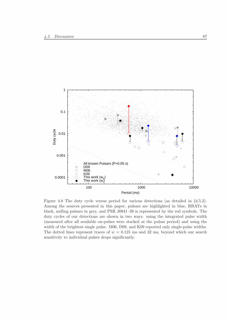
4.5. Discussion 87
0.0001
0.001
0.01
0.1
1
100 1000 10000
Dut
y cy
cle
Period (ms)
All known Pulsars (P>0.05 s)D09M06K09This work (ws)This work (wi)
Figure 4.8 The duty cycle versus period for various detections (as detailed in §4.5.2).Among the sources presented in this paper, pulsars are highlighted in blue, RRATs inblack, nulling pulsars in grey, and PSR J0941–39 is represented by the red symbols. Theduty cycles of our detections are shown in two ways: using the integrated pulse width(measured after all available on-pulses were stacked at the pulsar period) and using thewidth of the brightest single pulse. M06, D09, and K09 reported only single-pulse widths.The dotted lines represent traces of w = 0.125 ms and 32 ms, beyond which our searchsensitivity to individual pulses drops significantly.
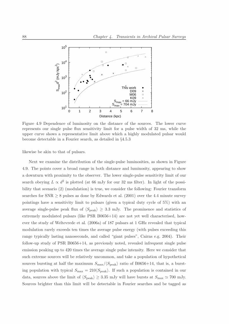
88 Chapter 4. Transients in Archival Pulsar Surveys
101
102
103
104
105
0 1 2 3 4 5 6 7 8
Sm
axd2 (
mJy
kpc
2 )
Distance (kpc)
This workD09M06K09
Smax = 66 mJySmax = 704 mJy
Figure 4.9 Dependence of luminosity on the distance of the sources. The lower curverepresents our single pulse flux sensitivity limit for a pulse width of 32 ms, while theupper curve shows a representative limit above which a highly modulated pulsar wouldbecome detectable in a Fourier search, as detailed in §4.5.3
likewise be akin to that of pulsars.
Next we examine the distribution of the single-pulse luminosities, as shown in Figure
4.9. The points cover a broad range in both distance and luminosity, appearing to show
a downturn with proximity to the observer. The lower single-pulse sensitivity limit of our
search obeying L ∝ d2 is plotted (at 66 mJy for our 32 ms filter). In light of the possi-
bility that scenario (2) (modulation) is true, we consider the following: Fourier transform
searches for SNR ≥ 8 pulses as done by Edwards et al. (2001) over the 4.4 minute survey
pointings have a sensitivity limit to pulsars (given a typical duty cycle of 5%) with an
average single-pulse peak flux of 〈Speak〉 ≥ 3.3 mJy. The prominence and statistics of
extremely modulated pulsars (like PSR B0656+14) are not yet well characterised, how-
ever the study of Weltevrede et al. (2006a) of 187 pulsars at 1 GHz revealed that typical
modulation rarely exceeds ten times the average pulse energy (with pulses exceeding this
range typically lasting nanoseconds, and called “giant pulses”, Cairns e.g. 2004). Their
follow-up study of PSR B0656+14, as previously noted, revealed infrequent single pulse
emission peaking up to 420 times the average single pulse intensity. Here we consider that
such extreme sources will be relatively uncommon, and take a population of hypothetical
sources bursting at half the maximum Smax/〈Speak〉 ratio of B0656+14, that is, a burst-
ing population with typical Smax = 210〈Speak〉. If such a population is contained in our
data, sources above the limit of 〈Speak〉 ≥ 3.35 mJy will have bursts at Smax ≃ 700 mJy.
Sources brighter than this limit will be detectable in Fourier searches and be tagged as
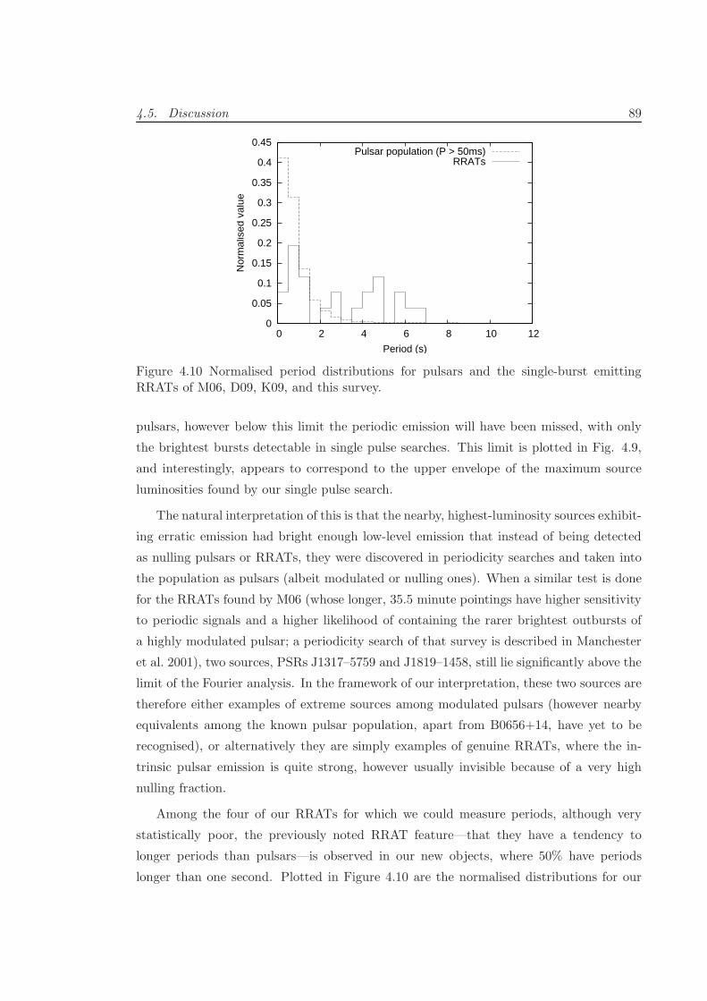
4.5. Discussion 89
0
0.05
0.1
0.15
0.2
0.25
0.3
0.35
0.4
0.45
0 2 4 6 8 10 12
Nor
mal
ised
val
ue
Period (s)
Pulsar population (P > 50ms)RRATs
Figure 4.10 Normalised period distributions for pulsars and the single-burst emittingRRATs of M06, D09, K09, and this survey.
pulsars, however below this limit the periodic emission will have been missed, with only
the brightest bursts detectable in single pulse searches. This limit is plotted in Fig. 4.9,
and interestingly, appears to correspond to the upper envelope of the maximum source
luminosities found by our single pulse search.
The natural interpretation of this is that the nearby, highest-luminosity sources exhibit-
ing erratic emission had bright enough low-level emission that instead of being detected
as nulling pulsars or RRATs, they were discovered in periodicity searches and taken into
the population as pulsars (albeit modulated or nulling ones). When a similar test is done
for the RRATs found by M06 (whose longer, 35.5 minute pointings have higher sensitivity
to periodic signals and a higher likelihood of containing the rarer brightest outbursts of
a highly modulated pulsar; a periodicity search of that survey is described in Manchester
et al. 2001), two sources, PSRs J1317–5759 and J1819–1458, still lie significantly above the
limit of the Fourier analysis. In the framework of our interpretation, these two sources are
therefore either examples of extreme sources among modulated pulsars (however nearby
equivalents among the known pulsar population, apart from B0656+14, have yet to be
recognised), or alternatively they are simply examples of genuine RRATs, where the in-
trinsic pulsar emission is quite strong, however usually invisible because of a very high
nulling fraction.
Among the four of our RRATs for which we could measure periods, although very
statistically poor, the previously noted RRAT feature—that they have a tendency to
longer periods than pulsars—is observed in our new objects, where 50% have periods
longer than one second. Plotted in Figure 4.10 are the normalised distributions for our
90 Chapter 4. Transients in Archival Pulsar Surveys
and the published “classic RRAT” sources as compared with the known pulsar population
for pulsars with P > 50 ms (to restrict the analysis to non-recycled pulsars). When a
Komolgorov-Smirnov test is run on the un-normalised distributions, it results in a high
probability, P = 0.999985 (> 4σ), that the distributions are not drawn from the same
parent population. Few pulsars have periods greater than P = 3 s and because sources
such as anomalous X-ray pulsars/magnetars/soft gamma-ray repeaters all have periods
greater than a few seconds, it is tempting to draw an association between such sources
and RRATs; the recent release of timing data on six RRATs by McLaughlin et al. (2009)
show a further similarity of RRATs to these other neutron star types in their placement
in the period-period derivative diagram, and a similar result in periodicity distribution
differences. However, the broad distribution of source periods and the presence of 7
RRATs with periods below one second suggests that a more basic factor in the population,
for instance age, which can create the observed tendency to longer periods. For the
RRATs which have had timing analysis done, all appear to have ages of a few times 105−6
years. However, the statistical analysis of McLaughlin et al. (2009), which compared
various derived RRAT and pulsar quantities, does not indicate a strong difference in the
distribution of RRAT and pulsar ages, though does indicate a strong probability that the
distribution of RRAT and pulsar magnetic field strengths are significantly different. There
appears to be no relation between RRAT period and distance from the galactic plane (a
proxy, albeit a loose one, for pulsar age).
The source PSR J0941–39 contributes a peculiar voice to this discussion, appearing
for hours, to possibly weeks at a time like a classic RRAT—erratically emitting single,
non-sequential pulses at a relatively constant rate—while at other times appearing as an
intense (∼ 10 mJy) pulsar with a < 10% nulling fraction, sub-pulse drift that is strongly
latitude dependent, as well as deep latitude-dependent modulation. The object appears
superficially to tie a close link between nulling phenomena and RRATs, possibly signifying
a pulsar which is in some way transitioning from a pulsar mode to an RRAT mode. If
this is the case, the source provides a link both between RRATs and pulsars as well as
a link to older, non-radio-emitting neutron stars—i.e. that the RRAT phase represents a
degradation of the radio emission mechanism before advancing beyond the radio pulsar
death line. As a timing solution is acquired for this pulsar, it will be interesting to note
whether it is of an advanced age. It is rather surprising how luminous this pulsar is, and
what a small nulling fraction it possesses when in its “pulsar” state. It is important to
note that the site of the RRAT emission is coincident with the three peaks of the profile
when the pulsar is on. Thus, the RRAT emission is from the same site as the normal
4.6. Summary 91
pulsar emission, again implying similar beaming fractions for the two states.
The properties of the new transients found in this search, and particularly of the five
new RRATs, give various indicators that RRAT behaviour is well described by either or
both of scenarios (2) or (3) above. The idea that observed RRAT behaviour may be an
observed consequence of extreme (> 99%) nulling is supported by the high nulling fraction
of the objects tagged as “nulling pulsars” above; while previously the “record” nulling frac-
tion was held by PSR B1713–40 at 95% (Wang et al. 2007), PSRs J1825–33, J1647–36, and
J1534–46 all have implied nulling fractions of more than 97%, telling us that these objects
may imply a “bridging population” of high-nulling-fraction pulsars, while objects with
higher nulling fractions (smaller and less frequent on-windows) exhibit RRAT behaviour.
A full statistical nulling fraction analysis of the Edwards et al. (2001) and Jacoby et al.
(2009) pulsars may indicate that the nulling fraction of the RRATs discovered in this
search fall naturally in the tail of pulsars with significant nulling fractions shown to exist
by Wang et al. (2007) in other surveys. This proposition, along with the lack of RRAT fea-
tures that are physically distinct from pulsars (except their period distribution)—including
their galactic and duty cycle distribution—point to a strong relationship to the “normal”
radio pulsar population. The story is complicated and strengthened by the apparent
mode-switching of PSR J0941–39, which lends significant support for scenario (3) in that
it is clear that the object in its RRAT mode is not simply a modulated pulsar, and it is
likewise clear that the object is both RRAT and pulsar in nature, signifying a transition
between the two populations and more speculatively, implying that nulling pulsars may
undergo stepped increases in their nulling fraction with age. The analyses of Wang et al.
(2007) indicate no correlation between nulling fraction and characteristic pulsar age, how-
ever the number of pulsars exhibiting nulls appears to increase with proximity to the radio
death line (see their Fig. 8). If all RRATs are relics of nulling pulsars, the broadening of
integrated pulse measurements supports the fact that despite their sparse emission, the
emitted pulses may still be exhibiting drifting or mode-changing phenomena.
4.6 Summary
We have re-examined the intermediate galactic latitude surveys of Edwards et al. (2001)
and Jacoby et al. (2009) for single pulses of radio emission of duration 0.125 < w <
32 milliseconds. This search revealed 14 intermittent sources which appear to be neutron
stars. Periods ranging 0.2 to 6.2 s were measured for 12 of these sources. While only four of
the objects could be detected retrospectively by Fourier search techniques, the remaining
10 exhibited intermittent emission behaviour akin to both extreme nulling pulsars and
92 Chapter 4. Transients in Archival Pulsar Surveys
the classic RRATs discovered by McLaughlin et al. (2006). The sensitivity of our search
techniques to bursts of lower dispersion measure allowed us to find objects which were
closer than those detected by previous searches.
The general properties of the new sources appear to paint details of the extreme in-
termittent and RRAT population that concur with having similar emission modes and
galactic distribution to pulsars, despite being significantly less emissive than the general
population. It was found that the duty cycle distribution of our detections mimics that of
pulsars. These similarities, and the discovery in this search of pulsars with extremely high
nulling fractions, lead us to suggest that RRATs may represent an extreme type of nulling
pulsar whose window of on-activity is shorter than the rotation period of the object, and
that the sources observed to exhibit RRAT behaviour are a natural extension of the tail
of pulsars observed with high nulling fractions. Furthermore, PSR J0941–39 appears to
oscillate between a clear “nulling pulsar” state and a more intermittent “RRAT” mode.
This source may represent the first detection of an object in transition from a bright pulsar
with an average nulling fraction to a single-bursting source, closely tying nulling pulsars
to RRATs and indicating a possible evolutionary progression. Further studies and timing
are warranted and upcoming on this object.
We conclude by noting that identifying RRATs is not a simple task, as they may
represent a mixed population of intrinsically single-pulsing pulsars and highly modulated
pulsars whose brightest single pulses singly exceed the system noise. Modulated pulsars
appearing as RRATs are expected to be few, as among the local population of pulsars,
PSR B0656+14 is currently the only pulsar known to be as modulated as the population
required for RRAT emission. Nearby pulsars which are part of such a population may in
the future be identified by pulse energy distribution studies of nearby highly modulated
pulsars, using long observations which have a chance of detecting the rarer brightest
outbursts from such objects. Statistical studies of these pulsars may help separate “true”
RRATs from simply highly modulated pulsars.
To discern the nature of RRATs, other extreme pulsar intermittents, and highly mod-
ulated objects, it will be critical in coming years to both identify more such sources, and
to continue timing analyses on the known sources to determine their relationship to other
neutron star populations. Of additional interest are the statistics of intermittent phe-
nomena in extreme nulling/modulated pulsars among the known pulsar population, the
analysis of which may reveal further insight into the relationship between regular pulsars
and the vast variety of intermittent behaviours observed in these equivocal neutron stars.
5Single Pulse Analysis in the The High Time
Resolution Universe Pulsar and Fast-Transient
Survey
Omnia mutantur, nos et mutamur in illis!
—M. Borbonius
In this chapter we describe the search for transient radio signals in the new High Time
Resolution Universe (HTRU) Survey. We present here: 1) the HTRU Survey’s single-pulse
search and follow-up strategy, and the software designed to perform the core single pulse
search, 2) a determination of the HTRU Survey’s sensitivity to single pulses, and 3) the
13 new neutron star discoveries made thus far with the single pulse pipeline. We return
to the “windowing” description of the previous chapter to explore RRATs and our new
detections in terms of emissivity timescales, and demonstrate the intermittent populations
that the HTRU Survey can explore, and note that the survey may discover more than 200
new sparsely emitting neutron stars by its completion.
5.1 Introduction
The High Time Resolution Universe Pulsar and Fast Transients (HTRU) Survey is the first
all-southern-sky survey for pulsars and fast transients using an all-digital backend, cover-
ing declinations δ < 10 (Keith et al. 2010; hereafter HTRU Paper 1). The survey employs
a new digital backend, the “Berkeley-Parkes-Swinburne Recorder” (hereafter BPSR), that
has been installed at Parkes Telescope for the 20 cm multibeam receiver (Staveley-Smith
et al. 1996). BPSR allows improved digitisation levels, and frequency and time resolution
over the previous analogue instrument. This affords the HTRU survey unprecedented
93
94 Chapter 5. Transients in the High Time Resolution Universe Survey
sensitivity to short-duration and highly dispersed single impulses of radio emission in the
southern sky. This chapter describes the techniques used in the survey to search for single
pulses. Because this survey required concurrent searches using periodicity and single-pulse
techniques, it affords the opportunity to explore efficient modes of search operation, at-
tempting to perform these techniques in parallel with a minimum of duplicated computing
effort.
The targets of our search are similar to those described in Sections 1.4.3, 1.4.4, and
4.1, and include RRATs, giant pulses from pulsars, radio bursts of extragalactic origin,
terrestrial impulses (e. g. Chap. 6) and other unanticipated, yet undetected sources of
celestial transient radio emission.
The HTRU intermediate (galactic longitudes −120 < l < 30, latitudes |b| < 15)
and high (covering declinations δ < +10 not covered by intermediate pointings) latitude
surveys share common areas of sky coverage to previous surveys which employed the
analogue filterbank installed on the Parkes Multibeam receiver.1 The “Parkes Multibeam
Survey” (Manchester et al. 2001) covered |b| < 5 with 35-minute pointings, and was
searched for single pulses by McLaughlin et al. (2006) and Keane et al. (2010), revealing
the bulk of the currently known RRAT population. Hereafter we refer to these searches
collectively as the PKSMB searches. At higher galactic latitudes, a single pulse search was
performed on the Jacoby et al. (2009) and Edwards et al. (2001) surveys, as presented in
Chapter 4. We refer to that search throughout this chapter as BSB, in reference to the
refereed publication in which the search was also described (Burke-Spolaor & Bailes 2010).
Despite the common sky coverage and high success rate of the BSB and PKSMB searches,
we nevertheless expect to discover any source of impulsive radio emission in these areas;
some pulsing radio sources may not have been previously detected due to the source’s low
event rate, insufficient sensitivity in previous surveys, or the improved dynamic range of
the BPSR observing system over the previous analogue filterbank system installed on the
Parkes multibeam receiver, whose dynamic range was hurt by√N -statistics (explored in
more detail in §5.2.2 below).
In this chapter we present the search methods, sensitivity, and current status of
the HTRU Survey single pulse search (§5.2), and report on initial discoveries for the
intermediate- and high-latitude surveys (§5.3). In §5.4, we determine why our discoveries
were not seen in the previous surveys of overlapping regions, present our new discoveries
in terms of the windowing description of pulsar intermittence presented in Chap. 4, and
make predictions for the sparsely-emitting radio neutron stars that the full HTRU survey
1Note: although no processing has yet commenced for the HTRU low-latitude survey, that survey willcover areas |b| < 3.5 and −80 < l < 30, with 70minutes per pointing.
5.2. The HTRU Survey’s Single-pulse (SP) Search 95
will uncover.
5.2 The HTRU Survey’s Single-pulse (SP) Search
5.2.1 Data Analysis Pipeline
Thus far all processing and analysis has been carried out using the “Green Machine”
supercomputer at the Swinburne Centre for Astrophysics and Supercomputing. This su-
percomputer is made up of ∼150 dual quad-core CPU nodes that accommodate large-scale
parallel and distributed processing. The pipeline employs several standard search tech-
niques (e. g. dedispersion and boxcar matched filtering), and several novel techniques
(independent-event identification and inspection, multi-beam coincidence matching, dis-
tributed computing). The basic methodology of the SP search is based on that described
in Chap. 4.
There are two main bottlenecks in the HTRU Survey’s single-pulse search. The first is
the computational load demanded by the dedispersion of our data, and the second is the
number of candidates which need to be manually assessed. The single-pulse data reduction
pipeline design includes schema that aim to abate both of these. First, we minimise the net
computational time of the periodicity and SP searches by integrating the SP search into the
hitrun processing pipeline introduced in HTRU Paper 1. By doing this, the interference
excision and dedispersion described in HTRU Paper 1 is done only once, producing each
data stream’s results simultaneously for use in the single-pulse search and the periodicity
search. As described below, the time series search for single pulses is performed while
each time series is still in the computer’s “random access memory”, and for each 9-minute
data stream adds <2.5 minutes of processing time onto the total ∼3-hour timescale for the
hitrun Fourier-based pipeline. We stress that the added computational load of including
a single pulse search to a traditional Fourier search is negligible.
We address the issue of large candidate numbers by identifying independent events
across multiple dispersion, boxcar filter trials, and beams, and by performing a simple
threshold-based interference zapping. The simultaneous processing and viewing of data
from multiple beams decreases the occurrence of candidates caused by low-level, local
interference and greatly increases the speed at which the manual assessment of a candidate
can be made. However, due to limited computational resources, we cannot store all 13
beams on one node, requiring the use of a monitor to track and collect beams from each
pointing as they are processed.
The single-beam SP search and the multibeam data monitor are described below.
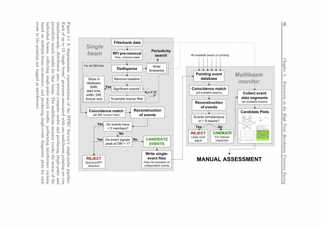
96Chapter
5.
Transien
tsin
theHigh
Tim
eReso
lutio
nUniverse
Survey
For all DM trials
Filterbank data
RFI pre-removalTime, channel mask
Remove baseline
Significant events?
Store in
database:
SNR,
start time,
width, DM,
boxcar size N-sample boxcar filter
Dedisperse
Coincidence match(all DM, boxcar trials)
Reconstruction
of events
Periodicity
search
Do event signals
peak at DM < 1?
Do events have
< 3 members?
REJECTSpurious/RFI
detection
No
Yes
Yes CANDIDATE
EVENTS
No
Write single-
event filesFiles list members of
independent events
Write
timeseries
Nb= 21,22,
… 29
Yes
Single
beam
Multibeam
monitor
Pointing event
database
Coincidence match(all available beams)
Reconstruction
of events
All available beams in pointing
Events simultaneous
in > 9 beams?
Yes No
CANDIDATEFor manual
inspection
REJECTLikely local
signal
Collect event
data segments(all available beams)
Candidate Plots
MANUAL ASSESSMENT
Figu
re5.1
Adiagram
matic
represen
tationof
theHTRU
Survey
’ssin
gle-pulse
pipelin
e.Each
ofupto
13“sin
glebeam
”processes
associated
with
onemultib
eampoin
tingare
run
simultan
eously,
distrib
uted
onto
severalcom
pute
nodes
andproducin
gsin
gle-pulse
and
perio
dicity
searchresu
ltsfor
that
beam
.Themultib
eammon
itortrack
sthestatu
sof
the
individual
beam
s,collectin
gsin
gle-pulse
searchresu
lts,perform
inginterferen
ceexcision
based
onmultip
le-beam
occu
rrence,
andproducin
gsin
gle-eventdiagn
osticplots
foreach
eventin
thepoin
tingnot
taggedas
interferen
ce.
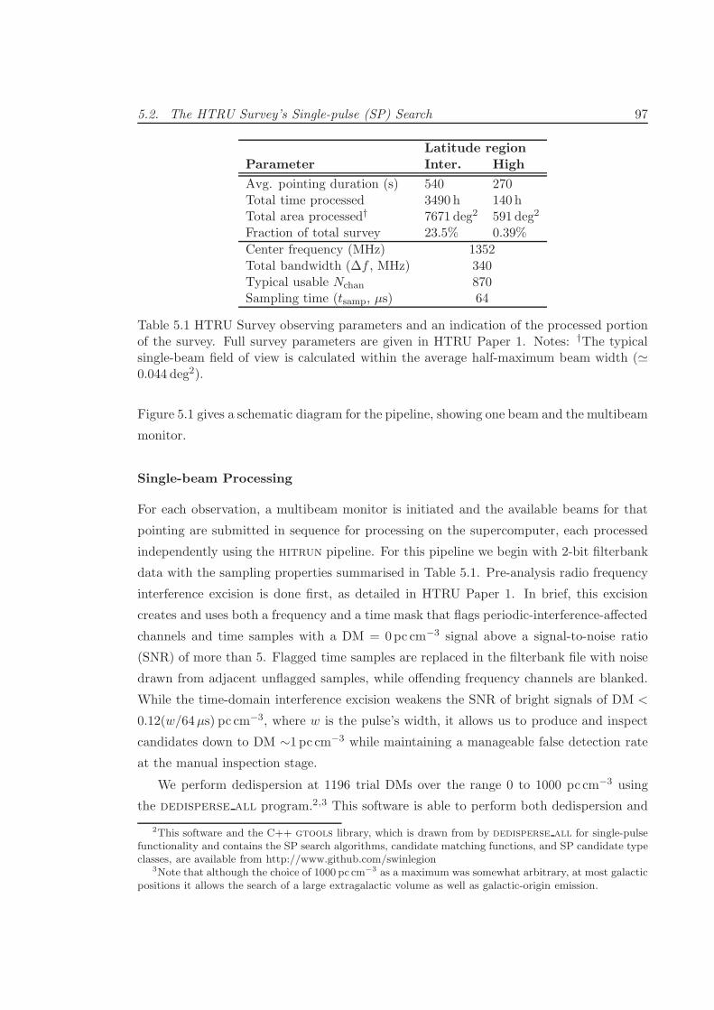
5.2. The HTRU Survey’s Single-pulse (SP) Search 97
Latitude regionParameter Inter. High
Avg. pointing duration (s) 540 270Total time processed 3490 h 140 hTotal area processed† 7671 deg2 591 deg2
Fraction of total survey 23.5% 0.39%
Center frequency (MHz) 1352Total bandwidth (∆f , MHz) 340Typical usable Nchan 870Sampling time (tsamp, µs) 64
Table 5.1 HTRU Survey observing parameters and an indication of the processed portionof the survey. Full survey parameters are given in HTRU Paper 1. Notes: †The typicalsingle-beam field of view is calculated within the average half-maximum beam width (≃0.044 deg2).
Figure 5.1 gives a schematic diagram for the pipeline, showing one beam and the multibeam
monitor.
Single-beam Processing
For each observation, a multibeam monitor is initiated and the available beams for that
pointing are submitted in sequence for processing on the supercomputer, each processed
independently using the hitrun pipeline. For this pipeline we begin with 2-bit filterbank
data with the sampling properties summarised in Table 5.1. Pre-analysis radio frequency
interference excision is done first, as detailed in HTRU Paper 1. In brief, this excision
creates and uses both a frequency and a time mask that flags periodic-interference-affected
channels and time samples with a DM = 0pc cm−3 signal above a signal-to-noise ratio
(SNR) of more than 5. Flagged time samples are replaced in the filterbank file with noise
drawn from adjacent unflagged samples, while offending frequency channels are blanked.
While the time-domain interference excision weakens the SNR of bright signals of DM <
0.12(w/64µs) pc cm−3, where w is the pulse’s width, it allows us to produce and inspect
candidates down to DM ∼1 pc cm−3 while maintaining a manageable false detection rate
at the manual inspection stage.
We perform dedispersion at 1196 trial DMs over the range 0 to 1000 pc cm−3 using
the dedisperse all program.2,3 This software is able to perform both dedispersion and
2This software and the C++ gtools library, which is drawn from by dedisperse all for single-pulsefunctionality and contains the SP search algorithms, candidate matching functions, and SP candidate typeclasses, are available from http://www.github.com/swinlegion
3Note that although the choice of 1000 pc cm−3 as a maximum was somewhat arbitrary, at most galacticpositions it allows the search of a large extragalactic volume as well as galactic-origin emission.
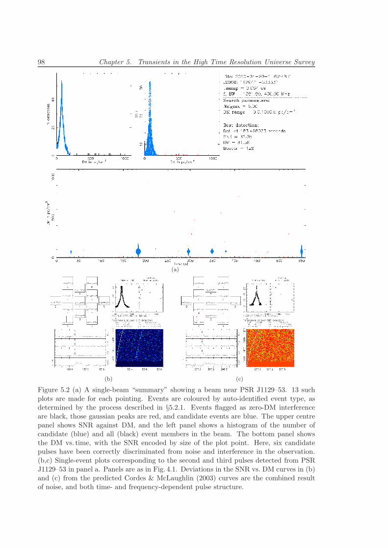
98 Chapter 5. Transients in the High Time Resolution Universe Survey
(a)
(b) (c)
Figure 5.2 (a) A single-beam “summary” showing a beam near PSR J1129–53. 13 suchplots are made for each pointing. Events are coloured by auto-identified event type, asdetermined by the process described in §5.2.1. Events flagged as zero-DM interferenceare black, those gaussian peaks are red, and candidate events are blue. The upper centrepanel shows SNR against DM, and the left panel shows a histogram of the number ofcandidate (blue) and all (black) event members in the beam. The bottom panel showsthe DM vs. time, with the SNR encoded by size of the plot point. Here, six candidatepulses have been correctly discriminated from noise and interference in the observation.(b,c) Single-event plots corresponding to the second and third pulses detected from PSRJ1129–53 in panel a. Panels are as in Fig. 4.1. Deviations in the SNR vs. DM curves in (b)and (c) from the predicted Cordes & McLaughlin (2003) curves are the combined resultof noise, and both time- and frequency-dependent pulse structure.
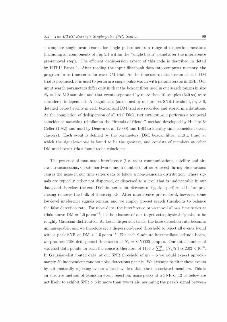
5.2. The HTRU Survey’s Single-pulse (SP) Search 99
a complete single-beam search for single pulses across a range of dispersion measures
(including all components of Fig. 5.1 within the “single beam” panel after the interference
pre-removal step). The efficient dedispersion aspect of this code is described in detail
by HTRU Paper 1. After reading the input filterbank data into computer memory, the
program forms time series for each DM trial. As the time series data stream at each DM
trial is produced, it is used to perform a single pulse search with parameters as in BSB. Our
input search parameters differ only in that the boxcar filter used in our search ranges in size
Nb = 1 to 512 samples, and that events separated by more than 10 samples (640 µs) were
considered independent. All significant (as defined by our pre-set SNR threshold, mt > 6,
detailed below) events in each boxcar and DM trial are recorded and stored in a database.
At the completion of dedispersion of all trial DMs, dedisperse all performs a temporal
coincidence matching (similar to the “friends-of-friends” method developed by Huchra &
Geller (1982) and used by Deneva et al. (2009) and BSB to identify time-coincident event
clusters). Each event is defined by the parameters (DM, boxcar filter, width, time) at
which the signal-to-noise is found to be the greatest, and consists of members at other
DM and boxcar trials found to be coincident.
The presence of man-made interference (i. e. radar communications, satellite and air-
craft transmissions, on-site hardware, and a number of other sources) during observations
causes the noise in our time series data to follow a non-Gaussian distribution. These sig-
nals are typically either not dispersed, or dispersed to a level that is undetectable in our
data, and therefore the zero-DM timeseries interference mitigation performed before pro-
cessing removes the bulk of these signals. After interference pre-removal, however, some
low-level inteference signals remain, and we employ pre-set search thresholds to balance
the false detection rate. For most data, the interference pre-removal allows time series at
trials above DM = 1.5 pc cm−3, in the absence of our target astrophysical signals, to be
roughly Gaussian-distributed. At lower dispersion trials, the false detection rate becomes
unmanageable, and we therefore set a dispersion-based threshold to reject all events found
with a peak SNR at DM < 1.5 pc cm−3. For each 9-minute intermediate latitude beam,
we produce 1196 dedispersed time series of Ns ≃ 8450000 samples. Our total number of
searched data points for each file consists therefore of 1196×∑9i=0(Ns/2
i) ≃ 2.02 × 10¹⁰.
In Gaussian-distributed data, at our SNR threshold of mt = 6 we would expect approxi-
mately 50 independent random noise detections per file. We attempt to filter these events
by automatically rejecting events which have less than three associated members. This is
an effective method of Gaussian event rejection; noise peaks at a SNR of 12 or below are
not likely to exhibit SNR > 6 in more than two trials, assuming the peak’s signal between
100 Chapter 5. Transients in the High Time Resolution Universe Survey
DM steps and boxcar trials drops by at least√2. Furthermore, the number of statis-
tically random events above SNR = 12 is negligible, even when considering analysis of
the full HTRU intermediate latitude survey. This strategy weakly impacts our sensitivity
to events of w = Nbtsamp that have SNR . 12. However, in concert these event-match-
based candidate rejection typically reduces the number of candidates by a further factor
of ∼100–1000, and much more for data badly affected by interference. In Fig. 5.2, we
show the two visual inspection plots used for manual candidate descrimination. For the
observation displayed, the telescope was pointed at PSR J1129–53, a known RRAT (BSB).
The six pulses emitted by the pulsar in this pointing were correctly discriminated by the
software from zero-dispersion interference and from spurious peaks in the data.
All non-interference events are then written to disk by dedisperse all, producing
one ASCII file per event, in which all members of that event are listed. At this stage, the
single-pulse events for the beam are gathered by the multibeam data monitor associated
with the beam’s pointing. The time series are written to disk, stored for use in the
periodicity search and for later access by the multibeam data monitor.
Multibeam Data Monitor
As single-pulse events are produced for all the beams associated with one pointing, the
multibeam monitor for that pointing collects the events and performs a temporal coinci-
dence match of identical form to that done by dedisperse all, however it is performed
for events from different beams.
The Parkes 20cm multibeam receiving system was described in §4.2, but is reviewed
in brief here. The system allows the simultaneous observation of 13 positions on the
sky with approximately 30 arcminutes between beam positions, and each beam has a
sensitivity fall-off on scales of <30 arcminutes from its pointing centre (Staveley-Smith
et al. 1996). Pointlike radio sources boresight to the telescope pointing direction will
therefore typically be detected in a maximum of three beams of the receiver. Particularly
luminous objects like the Vela Pulsar, which emits single pulses up to ∼60 Jy, may detected
in up to ∼7 beams when ideally positioned in the multibeam field. Typically, signals of
sufficient brightness to appear in all beams at similar intensity, i. e. through a far sidelobe
of the telescope, are generated by terrestrial or near-Earth sources (such as satellites or
aircraft). Therefore, as in BSB, we do not inspect candidates which were detected in
more than nine of the thirteen beams. This filter decreases our sensitivity to the type of
impulses described in Chap. 6, however there is significant benefit gained through decrease
in the false detection rate per pointing. A targeted search for the objects of Chapter 6
5.2. The HTRU Survey’s Single-pulse (SP) Search 101
is planned for the near future. All events occurring in nine beams or less are imaged as
described in BSB, collecting the relevant filterbank and time series data from the original
on-disk location of the single beams. When both single-pulse and pulsar searches have
been completed, the data is freed for removal from disk.
Finally, a pointing’s result plots (i. e. those for individual beams and events as in
Fig. 5.2) are manually assessed to determine whether they contain a detection of interest.
The “beam summary” plot has superiour sensitivity to objects emitting multiple pulses
with signals at or just exceeding the detection threshold, while the single-event plots allow a
user swift discrimination between interesting candidates and falsely-identified interference
or noise. During the manual inspection stage, results are also compared with the most
up-to-date version of the Australia Telescope National Facility Pulsar Catalogue originally
published by Manchester et al. (2005).
5.2.2 Search Sensitivity
The sky coverage of the HTRU survey affords improved sensitivity in overlapping regions
for previous blind single-pulse searches of the southern sky. Particularly for the HTRU
intermediate latitude survey, we have direct overlap with the areas searched by BSB and
PKSMB. Here we calculate our sensitivity to transient events and make a comparison to
these surveys.
Instrumental and interstellar pulse broadening serves to weaken the SNR of the pulse
from its signal at the pulse’s intrinsic width, wi. All instrumental broadening effects are in
principle avoidable, therefore the back-end design of any observing system aims to reach
the scatter-broadening limit, as this is the theoretical best that a pulsar/transients survey
can achieve. As noted in HTRU Paper 1, for a large range in dispersion measures the
improved time and frequency resolutions of the HTRU survey causes pulse broadening
from interstellar propagation to dominate over intrachannel dispersion-measure broaden-
ing (tch). Using the empirical DM-scatter broadening relation given by Bhat et al. (2004),
we note that scatter broadening (tscat) typically dominates over hardware-induced smear-
ing above a DM of ∼230 pc cm−3 for the HTRU survey. To calculate our sensitivity to
single pulses, we take these pulse-scattering and broadening effects into account.
Following Deneva et al. (2009), the observed pulse width depends on wi and various
pulse-broadening effects by w = (w2i +t
2ch+t
2scat+t
2samp)
0.5. Note that our step size between
DM trials is chosen such that the broadening due to an error in DM is small compared to
other broadening effects. Our sensitivity limit for the intrinsic peak flux density of single
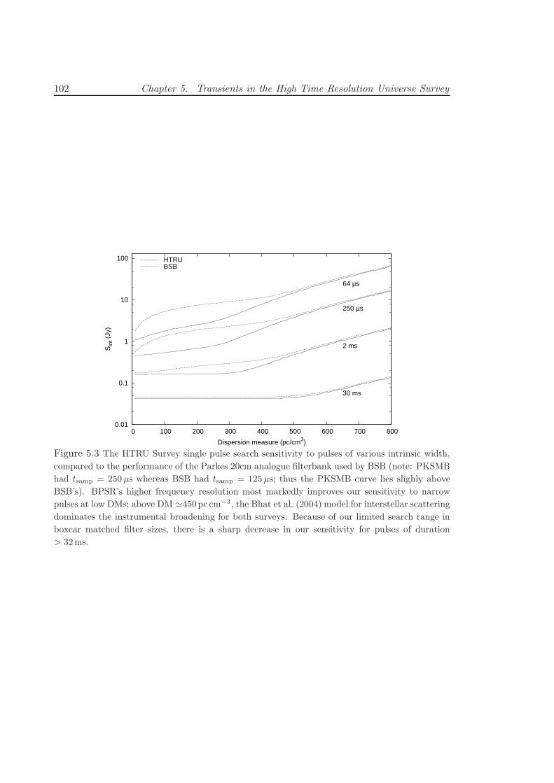
102 Chapter 5. Transients in the High Time Resolution Universe Survey
0.01
0.1
1
10
100
0 100 200 300 400 500 600 700 800
Sin
t (Jy
)
Dispersion measure (pc/cm3)
64 µs
250 µs
2 ms
30 ms
HTRUBSB
Figure 5.3 The HTRU Survey single pulse search sensitivity to pulses of various intrinsic width,
compared to the performance of the Parkes 20cm analogue filterbank used by BSB (note: PKSMB
had tsamp = 250µs whereas BSB had tsamp = 125µs; thus the PKSMB curve lies slighly above
BSB’s). BPSR’s higher frequency resolution most markedly improves our sensitivity to narrow
pulses at low DMs; above DM ≃450pc cm−3, the Bhat et al. (2004) model for interstellar scattering
dominates the instrumental broadening for both surveys. Because of our limited search range in
boxcar matched filter sizes, there is a sharp decrease in our sensitivity for pulses of duration
> 32ms.
5.2. The HTRU Survey’s Single-pulse (SP) Search 103
pulses with observed duration w = Nb · tsamp is then
Sint ≥ Sobs ·w
wi; Sobs =
mt Tsys β
G√
Npw∆f(5.1)
(c.f. Lorimer & Kramer 2004), where Tsys ≃ 23K is the system temperature of the multi-
beam system, G is the telescope gain (ranging 0.735–0.581 KJy−1 from the central to outer
beams), and Np = 2 is the number of summed polarisations in the data. β is a factor of
order ∼1 that is included to represent signal losses due to system imperfections. Fig. 5.3,
we indicate our sensitivity to single pulses of various durations as a function of dispersion
measure, and in comparison to the sensitivities of PKSMB and BSB.
The 2-bit digitisation levels of the BPSR instrument and large number of frequency
channels result in the increased dynamic range capabilities over the previous Parkes ana-
logue filterbank. In HTRU Survey data, each frequency channel is sampled at levels
defined l = 0, 1, 2, 3. This produces dedispersed time series with integer values ranging
0 to 2610. When processed using the dedisperse all software, for efficient data size
when written to disk, and to a lesser extent for efficient processing (see HTRU Paper 1),
input data values get transformed as (lNchan/16)−128. In the absence of interference, the
mean bit level should be 1.5. The mean of the time series produced by dedisperse all
should therefore be µ ≃ −46.5, with a data maximum value of 35 (when all channels have
l = 3). We made empirical measurements of the mean and standard deviation (σ) of data
judged by eye to not be strongly affected by interference. We found µ = −48 and σ = 2
for interference-clean files, in reasonable agreement with the expected mean. With these
values, we calculate the highest achievable SNR in the HTRU Survey data for pulses with
w = tsamp to be (35− µ)/σ = 41.5. This is in good agreement with the SNR of saturated
interference pulses observed in DM = 0pc cm−3 time series. For the 1-bit, 96-channel
analogue filterbank, the maximum SNR may be calculated analytically. In this system,
data uninterrupted by interference has an equal probability of having bit level l = 0 (“off”)
or l = 1 (“on”); that is, Pon = Poff = 0.5. The data values in this system are described
by a binomial probability distribution, with the probability of being in a state with non
on-channels and noff off-channels (non + noff = Nchan = 96) given by:
Pstate =Nchan!
non!(Nchans − non)!(Pon)
non(1− Pon)Nchan−non (5.2)
This function is a Gaussian with µ = 48 and σ = 5. The theoretical maximum SNR of
this system at w = tsamp is then (96 − µ)/σ = 9.6. Again, this agrees with saturated
interference signals observed in data from this system. The differences in dynamic range
104 Chapter 5. Transients in the High Time Resolution Universe Survey
for these systems do not strictly impact the flux sensitivity of a single-pulse search, however
the HTRU Survey’s increase in dynamic range will affect the manual inspection stage by
allowing detections of potentially very bright, narrow pulses to be more clearly discernible
from noise or non-Gaussian statistics in the observation. This effect is more acute for
pulses of width close to the sampling time of each analogue filterbank survey.
The improved resolution of the HTRU Survey is clearly beneficial for the detection of
RRATs, which are known to have narrow pulse widths (e. g. McLaughlin et al. 2006), and
other pulsars or extragalactic impulse emitters with durations w . 10ms and dispersion
measures of DM . 360 pc cm−3. For DM > 360 pc cm−3, we do not expect to see a large
number of new RRATs for several reasons; first, we do not have a considerable increase
in sensitivity over the previous surveys for these DMs, and the number RRATs above this
DM represents only ∼10% of the known RRAT population. Additionally, for |b| < 5, the
35-minute pointing duration of PKSMB searches afford a greater probability of detection
of low-pulsation rate events over our 8.5-minute observations of these areas, and we offer
minimal improvements for the capability of detection of these objects. At higher latitudes,
for the bulk of pointing positions in the HTRU Survey the number density of electrons in
the Galaxy is insufficient to produce dispersion measures much greater than 360 pc cm−3
(Cordes & Lazio 2002). For these reasons, we expect most new rotating radio transient
and deep nulling pulsar discoveries to be at dispersion measures DM < 360 pc cm−3. As
detailed in §5.4.1, this seems to hold true for the initial discoveries.
5.2.3 Current Processing Status
The current status of the HTRU Survey processing is summarised in the upper panel of
Table 5.1. The processing reported in this paper includes only pointings from the HTRU
intermediate and high latitude surveys. The survey coverage to date is not contiguous
over all galactic regions. For later interpretation of the galactic distribution of our dis-
coveries, we indicate the total observation time of the processed pointings as a function
of sky position in Figure 5.4. In total, 22,273 and 1,718 beams have been processed out
of the 95,056 and 443,287 total beams of the intermediate and high latitude surveys, re-
spectively. Approximately 160 incomplete survey pointings of shorter duration have also
been processed. Nevertheless, the bulk of observing time reported in this paper has been
spent at galactic latitudes |b| < 15.
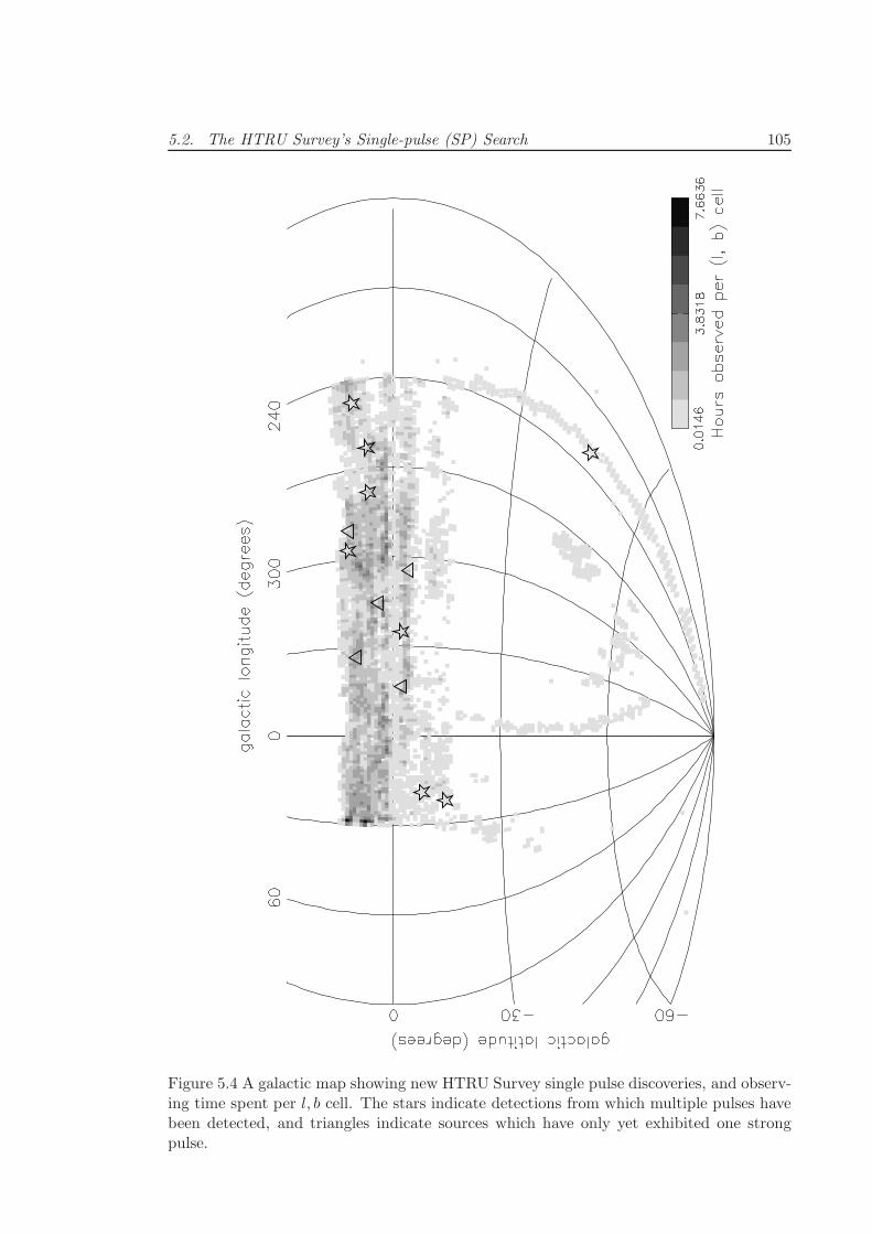
5.2. The HTRU Survey’s Single-pulse (SP) Search 105
Figure 5.4 A galactic map showing new HTRU Survey single pulse discoveries, and observ-ing time spent per l, b cell. The stars indicate detections from which multiple pulses havebeen detected, and triangles indicate sources which have only yet exhibited one strongpulse.
106 Chapter 5. Transients in the High Time Resolution Universe Survey
5.2.4 Candidate Ranking and Follow-up Strategy
Because telescope time is a valuable resource, the infrequent emission from RRATs and
extreme nullers make it scientifically inefficient to perform extensive follow-up for all of
the candidate pulses discovered in our search, many of which will not be genuine celestial
objects. We employ a follow-up prioritisation scheme to provide efficient scientific return
with available observing time. Based on the strength of the candidate in various panels of
the manual inspection plots and the number of detections at a similar DM in a pointing
(recall Fig. 4.1 and Fig. 5.2), candidates are ranked multi-pulse (two or more strong pulses
detected at similar DM), strong (≥2 weak pulses, or one convincing pulse detected, that
is with a SNR > 7 and exhibiting a characteristic signature in the SNR vs. DM plot,
e. g. as explored by Cordes & McLaughlin 2003), or weak (candidate’s time series shows
a detection at non-zero DM but is poorly supported by data in other inspection panels
and/or has SNR < 7). Weak candidates outnumber those ranked strong and multi-
pulse by a factor of more than two. In scheduling follow-up time, all candidates are
observed for a duration equal to that of the discovery pointing. Strong and multi-pulse
candidates are of higher priority. If weak detections are not seen in the initial follow-up
pointing, they are not tracked in further follow-up observations. We do not include these
detections in this report due to their highly uncertain nature, however we preserve them in
a database for posterity, taking into consideration that further weak detections in future
pulsar surveys of the same sky area could cross-correlate their findings with our weak,
unconfirmed detections (e. g. as will be possible with the HTRU Survey’s low-latitude
survey, and potentially with future Australian Square Kilometre Array Pathfinder/Square
Kilometre Array surveys). Multi-pulse and strong candidates not seen in initial follow-up
are observed again for a duration of three times the discovery pointing. We note that the
inactivity states in nulling pulsars has a broad range of timescales; on one extreme, RRATs
have been observed to emit single pulses separated by up to 3.25 hours (McLaughlin et al.
2006), and on another extreme, emission from some pulsars has been observed to turn
off for up to 5 days. Our ranking levels are set such that these categories are highly
unlikely to contain detections of spurious noise. We include all strong and multi-pulse
candidates in this report whether or not they are detected in follow-up pointings, with
the strong caveat that these objects essentially remain unconfirmed, and care must be
taken in including these objects in statistical or categorical transients studies. Objects
not detected in follow-up observations are distinguished in Table 5.2 by a limit instead of
a measurement of χ; this reflects that non-detections of these discoveries are used only to
place limits on χ for the object. Only one multi-pulse object has yet not been detected in
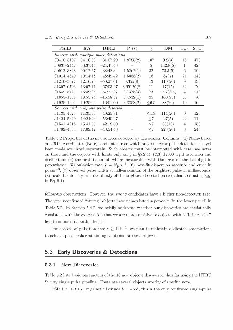
5.3. Early Discoveries & Detections 107
PSRJ RAJ DECJ P (s) χ DM weff Smax
Sources with multiple-pulse detectionsJ0410–3107 04:10:39 –31:07:29 1.8785(2) 107 9.2(3) 18 470J0837–2447 08:37:44 –24:47:48 – 5 142.8(5) 1 420J0912–3848 09:12:27 –38:48:34 1.5262(1) 32 73.3(5) 6 190J1014–4849 10:14:18 –48:49:42 1.5088(2) 16 87(7) 21 140J1216–5027 12:16:20 –50:27:01 6.355(9) 13 110(20) 9 130J1307–6703 13:07:41 –67:03:27 3.65120(8) 11 47(15) 32 70J1549–5721 15:49:05 –57:21:37 0.7375(3) 73 17.7(3.5) 4 210J1855–1558 18:55:24 –15:58:57 3.4532(1) 25 160(25) 65 50J1925–1601 19:25:06 –16:01:00 3.8858(2) ≤6.5 88(20) 10 160
Sources with only one pulse detectedJ1135–4925 11:35:56 –49:25:31 – ≤1.3 114(20) 9 120J1424–5640 14:24:23 –56:40:47 – ≤7 27(5) 22 110J1541–4218 15:41:55 –42:18:50 – ≤7 60(10) 4 150J1709–4354 17:09:47 –43:54:43 – ≤7 228(20) 3 240
Table 5.2 Properties of the new sources detected by this search. Columns: (1) Name basedon J2000 coordinates (Note, candidates from which only one clear pulse detection has yetbeen made are listed separately. Such objects must be interpreted with care; see noteson these and the objects with limits only on χ in §5.2.4); (2,3) J2000 right ascension anddeclination; (4) the best-fit period, where measurable, with the error on the last digit inparentheses; (5) pulsation rate χ = Np h
−1; (6) best-fit dispersion measure and error inpc cm−3; (7) observed pulse width at half-maximum of the brightest pulse in milliseconds;(8) peak flux density in units of mJy of the brightest detected pulse (calculated using Sobsin Eq. 5.1).
follow-up observations. However, the strong candidates have a higher non-detection rate.
The yet-unconfirmed “strong” objects have names listed separately (in the lower panel) in
Table 5.2. In Section 5.4.2, we briefly addresses whether our discoveries are statistically
consistent with the expectation that we are more sensitive to objects with “off-timescales”
less than our observation length.
For objects of pulsation rate χ ≥ 40 h−1, we plan to maintain dedicated observations
to achieve phase-coherent timing solutions for these objects.
5.3 Early Discoveries & Detections
5.3.1 New Discoveries
Table 5.2 lists basic parameters of the 13 new objects discovered thus far using the HTRU
Survey single pulse pipeline. There are several objects worthy of specific note.
PSR J0410–3107, at galactic latitude b = −56, this is the only confirmed single-pulse
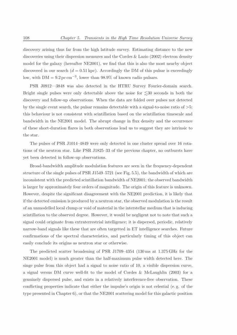
108 Chapter 5. Transients in the High Time Resolution Universe Survey
discovery arising thus far from the high latitude survey. Estimating distance to the new
discoveries using their dispersion measures and the Cordes & Lazio (2002) electron density
model for the galaxy (hereafter NE2001), we find that this is also the most nearby object
discovered in our search (d = 0.51 kpc). Accordingly the DM of this pulsar is exceedingly
low, with DM = 9.2 pc cm−3, lower than 98.9% of known radio pulsars.
PSR J0912—3848 was also detected in the HTRU Survey Fourier-domain search.
Bright single pulses were only detectable above the noise for .30 seconds in both the
discovery and follow-up observations. When the data are folded over pulses not detected
by the single event search, the pulsar remains detectable with a signal-to-noise ratio of >5;
this behaviour is not consistent with scintillation based on the scintillation timescale and
bandwidth in the NE2001 model. The abrupt change in flux density and the occurrence
of these short-duration flares in both observations lead us to suggest they are intrinsic to
the star.
The pulses of PSR J1014–4849 were only detected in one cluster spread over 16 rota-
tions of the neutron star. Like PSR J1825–33 of the previous chapter, no outbursts have
yet been detected in follow-up observations.
Broad-bandwidth amplitude modulation features are seen in the frequency-dependent
structure of the single pulses of PSR J1549–5721 (see Fig. 5.5), the bandwidth of which are
inconsistent with the predicted scintillation bandwidth of NE2001; the observed bandwidth
is larger by approximately four orders of magnitude. The origin of this feature is unknown.
However, despite the significant disagreement with the NE2001 prediction, it is likely that
if the detected emission is produced by a neutron star, the observed modulation is the result
of an unmodelled local clump or void of material in the interstellar medium that is inducing
scintillation to the observed degree. However, it would be negligent not to note that such a
signal could originate from extraterrestrial intelligence; it is dispersed, periodic, relatively
narrow-band signals like these that are often targetted in ET intelligence searches. Future
confirmations of the spectral characteristics, and particularly timing of this object can
easily conclude its origins as neutron star or otherwise.
The predicted scatter broadening of PSR J1709–4354 (130ms at 1.375GHz for the
NE2001 model) is much greater than the half-maximum pulse width detected here. The
singe pulse from this object had a signal to noise ratio of 10, a visible dispersion curve,
a signal versus DM curve well-fit to the model of Cordes & McLaughlin (2003) for a
genuinely dispersed pulse, and exists in a relatively interference-free observation. These
conflicting properties indicate that either the impulse’s origin is not celestial (e. g. of the
type presented in Chapter 6), or that the NE2001 scattering model for this galactic position
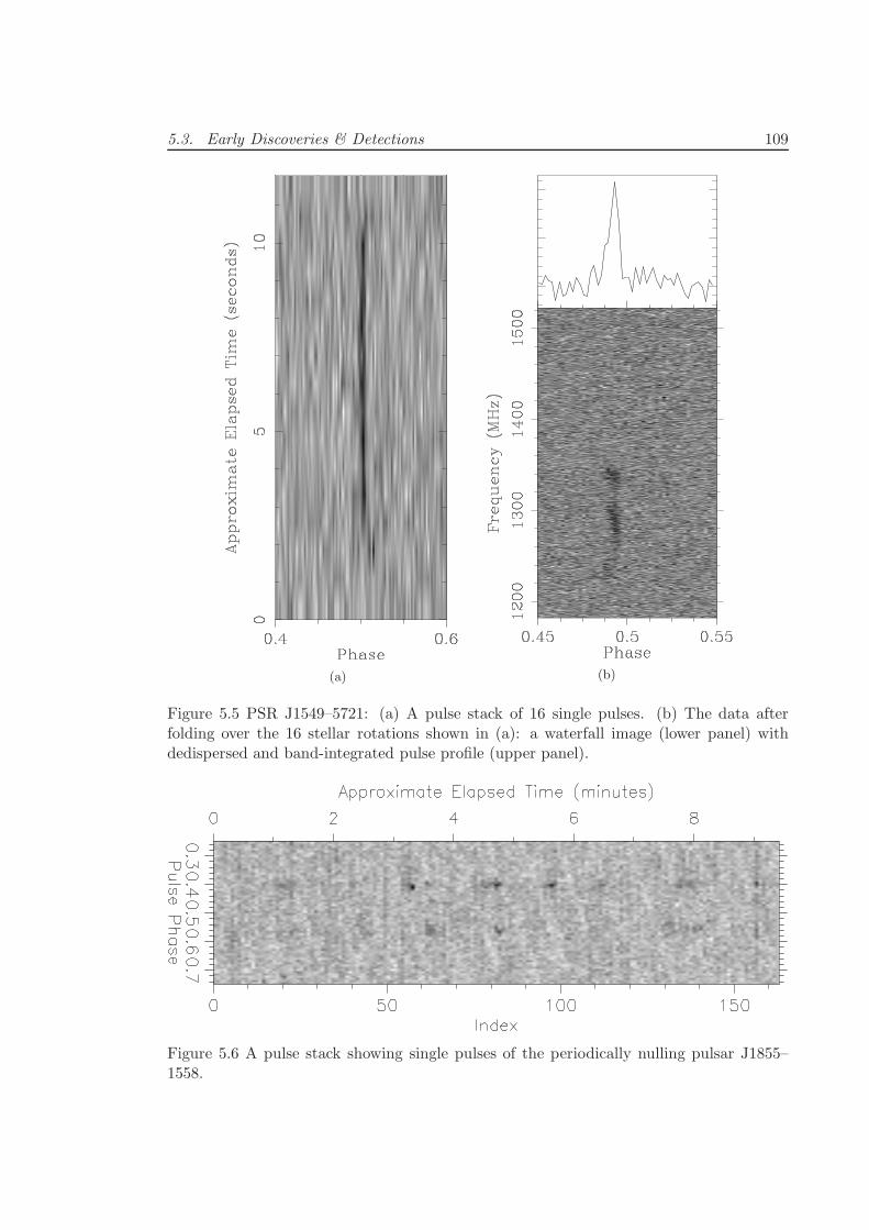
5.3. Early Discoveries & Detections 109
(a) (b)
Figure 5.5 PSR J1549–5721: (a) A pulse stack of 16 single pulses. (b) The data afterfolding over the 16 stellar rotations shown in (a): a waterfall image (lower panel) withdedispersed and band-integrated pulse profile (upper panel).
Figure 5.6 A pulse stack showing single pulses of the periodically nulling pulsar J1855–1558.
110 Chapter 5. Transients in the High Time Resolution Universe Survey
is incorrect. A redetection of this candidate would clarify the nature of this candidate,
however follow-up has not yet been performed.
PSR J1855–1558 appears to be exhibiting periodic nulling, drifting, and mode-changing
behaviours (Fig. 5.6). Despite a high nulling fraction, this object’s relatively frequent
emission renders it detectable in a Fourier search with a signal to noise ratio of ∼17 in the
8.5-minute survey and follow-up pointings.
5.3.2 Redetections of Known Pulsars and RRATs
The single pulse pipeline has detected approximately 55% of the known pulsars that could
be detected through Fourier searches of the HTRU Survey data. This offers a slight im-
provement in single-pulse detection rate over the search presented in the previous chapter,
perhaps a testament to the increased sensitivity to faint and narrow single pulses that this
survey’s hardware affords. The single-pulse properties of these objects will be analysed in
future work, so we will not detail them here.
We have processed 24 observations with pointing positions within 6 arcminutes (our
approximate half-power beam width) of published RRAT positions (i. e. from McLaughlin
et al. 2006, Keane et al. 2010, McLaughlin et al. 2009, Burke-Spolaor & Bailes 2010). Of
these 24, 13 RRATs were redetected. For 22 of 24 observations, the number of pulses seen
from each object were consistent with the expected number based on previously published
pulsation rates in the discovery observations of these objects (again, as drawn from the
BSB and PKSMB publications) and the observation length in our data. The two notably
different detection rates were of RRATs J1753–38 (BSB; 4 expected and > 15 seen) and
J1819–1458 (McLaughlin et al. 2006; 3 expected and 10 seen). PSR J1819–1458 has been
recently noted to exhibit small variations in pulsation rate (and larger ones associated
with glitches Lyne et al. 2009), and the detection rate observed here is consistent with
the range in χ reported by (Lyne et al. 2009). For PSR J1753–38, the higher detection
rate, detectability in a Fourier search with a signal-to-noise ratio of ∼13 (whereas it was
undetectable in a Fourier search of its original discovery data), and the slight increase
in Smax exhibited in our observations indicate that: 1) this pulsar’s emission appears to
simply be highly modulated, and does not have genuine deep nulls, and 2) our observing
position of the source is improved from that reported by BSB. Our positional offset was
0.1 degrees, suggesting an improved position of right ascension and declination 17:53:09,
–38:52:13 (J2000).
5.4. Discussion 111
5.4 Discussion
5.4.1 Our Discoveries in Archival Pulsar Surveys
As noted in §5.2.2, for the regions overlapping with previous surveys, we expected to
discover new objects mainly at DM . 360 pc cm−3. This appears to have been met,
however several of our detections appear to be of sufficient brightness that one would have
expected a detection in archival data. All of our discoveries except for PSR J0410–3107
and PSR J0837–2447 lie in regions previously covered by the surveys of Jacoby et al.
(2009), Edwards et al. (2001) and Manchester et al. (2001). The presence of pulses in
archival data—note that these surveys were performed 8-12 years ago—can add valuable
information about pulse rate changes over time, and potentially add data points to their
timing if a phase-coherent timing solution is obtained. We inspected pointings in these
surveys within one half-power beam width of our objects’ positions to determine the
detectability of our discoveries in the archival data. PSR J1307–6703 is the only one of
our discoveries which exhibits clear single pulse detections when the archival data are
dedispersed at the appropriate DM. We detect seven pulses of SNR > 5 in the 35-minute
archival observation for this object (giving a χ consistent within a factor of two of that
derived from the solitary detection in the HTRU Survey discovery pointing). It is from the
archival data that the period quoted in Table 5.2 was determined. While PSR J1855–1558
is not detectable in a Fourier search, it is marginally detectable when the archival data
are folded over the period given in Table 5.2.
We can investigate the reason for the non-detection of the remaining objects by first
estimating the signal loss due to the use of the analogue multibeam filterbank system used
by BSB and PKSMB, calculating the SNR that a pulse of equivalent width, DM, and ·Speak(as listed in Table 5.2) would have shown in the archival data. This analysis suggests that
even the brightest detected pulses in our data would result in only a marginal (SNR . 6)
detection in the analogue filterbank data for PSRs J1135–4925, J1541–4218, and J1709–
4354. For two out of four of the remaining objects at |b| > 5, for which the observation
length of the archival data was 4.4minutes, the non-detections could be accounted for by
the low probability that a pulse would occur during the time span of the observation for
objects with χ . 13.5 h−1. The remaining |b| > 5 objects, PSR J0912–3848 and PSR
J1014–4849, had clusters of sequential pulses rather than a smooth distribution of single
pulses. Although the per-hour pulsation rate is high for these objects, the average duration
of on-activity is short, the spacing between sequential pulse outbursts is &8 minutes. This
indicates that the non-detection of pulses in the archival data is consistent with a decreased
112 Chapter 5. Transients in the High Time Resolution Universe Survey
probability of the occurrence of a pulse outburst during the archival observations (if there
were they should have resulted in detections of SNR ∼8 and 11 for PSRs J0912–3848 and
J1014–4849, respectively). The effect of on- and off-timescales for object detectability will
be discussed further in Sec. 5.4.2.
The only remaining undetected objects are PSR J1549–5721 and PSR J1424–5640. We
have not yet performed follow-up observations on these objects, and so the archival data,
in which we would have expected to see detections of SNR > 7, serves only to place limits
on the pulsation rate and duration of off-activity in these objects. For PSR J1549–5721,
the non-detection in two archival pointings places a strong limit (zero pulses in ≥70m) on
these values.
5.4.2 Activity Timescales in Sparsely-emitting Neutron Stars
As reviewed in §4.5.1, the nature of RRATs, in particular their relationship to average
radio pulsars, is still somewhat a matter of debate. As explored briefly by SBS and
Keane et al. (2010), and in detail by Miller et al. (submitted), most objects discovered in
single pulse searches do appear to be genuinely “turned off” when they are not detected,
rather than being distant pulsars with atypically long-tailed pulse energy distributions;
one can discern these classifications by single-pulse energy statistics and the identification
of whether RRATs’ detectable pulses show a distinct log-normal distribution (Miller et al.
submitted).
For the objects exhibiting genuine nulls, the possibility of a clearly distinguished
“RRAT” class of neutron stars is beginning to break down, based on mounting evidence
that RRATs simply represent an extended tail of deeply-nulling objects in the nulling
population of pulsars. This is supported indirectly by the lack of distinction of RRAT and
pulsar Galactic and pulse width distributions (SBS) and further by the pulse energy dis-
tributions of RRATs, which as noted above tend to obey similar log-normal distributions
to average (nulling and non-nulling) pulsars. Furthermore, Keane (2010) note that the
“classic” definition of the RRAT class implied by the original McLaughlin et al. (2006)
publication is a neutron star for which r = mSP/mFFT > 1, where mSP is the SNR of the
brightest single pulse detected in an observation, and mFFT is the SNR of a Fast Fourier
Transform analysis for the pulsar in the same observation. This leads directly to the
inferrence that in fact whether a source is defined “RRAT” or “pulsar” is arbitrary, and
highly dependent on survey pointing length and pulsar period (McLaughlin & Cordes 2003,
Keane 2010), further obscuring RRAT intermittence as an exclusive physical phenomenon.
For selected objects, However, we do note that observed post-glitch behaviour of RRAT
5.4. Discussion 113
J1819–1458 (which showed a net decrease in spin-down luminosity post-glitch, rather than
the increase usually observed in pulsars Lyne et al. 2009) does set this particular object
apart from the pulsar population and drive the “exhausted magnetar” hypothesis put
forward by Lyne et al.
Nevertheless, given these facts we seek to more accurately incorporate our discoveries
and RRAT populations in general into the range of nulling and emissivity timescales
exhibited by radio pulsars. We explore a relevant “intermittence parameter space” here,
and review in Sec. 5.4.3 what effect survey parameters have on the selection of various
populations in this space.
As with the objects discovered in the search in Chap. 4, approximately 1/3 of our
single pulse pipeline discoveries exhibit distinct periods of on-activity, marked by bright
sequential pulses that are separated by longer intervals of either genuine nulls, or a de-
crease in intensity level sufficiently large that the object is undetectable through single
pulse or periodicity search techniques. The pulsation rate, χ, that is typically quoted
for single pulse discoveries poorly represents the emissivity of such objects and provides
insufficient information to assess the probability of detecting them during reobservation.
We return now to the “windowing” description of pulsar and RRAT emissivity that was
introduced in the previous chapter (recall Fig. 4.7), noting that the on and off states of
nulling pulsars often show characteristic timescales (Herfindal & Rankin 2007, Redman &
Rankin 2009, Wang et al. 2007) given by ton and toff , respectively. Quantifying intermit-
tence timescales in this way is more physically representative for pulsars of various nulling
fractions, better reflects the timescales associated with possible windowing phenomena,
and allows a more accurate exploration of selection effects for surveys of various length
(see §5.4.3). Here we use a definition of toff that is similar to the “null length” of Wang
et al. (2007). We define toff as the average time between the first pulse whose signal drops
below a set threshold (we use SNR > 5) and the next above that threshold. We define
ton as the average number of pulses (Non) above the same threshold, times the rotational
period of the object. Obviously, such an analysis is only valid for genuine nulling pul-
sars, and uninterrupted data spans of T ≫ ton + toff containing single pulse detections
of high significance would provide more accurate measurements of these quantities; for
our discoveries, most observations provide robust single pulse detections, although we are
insensitive to timescales ≫ 9minutes. We nevertheless make estimates of (or place limits
on, in observations where no timescales are measureable because they appear greater than
our data span) the average ton, toff for our discoveries based on all available data.
The nulling fraction of a pulsar is only valid in this analysis when measured over a
114 Chapter 5. Transients in the High Time Resolution Universe Survey
timescale far exceeding one activity cycle of the object, which is given by a length ton+toff .
Below we generically represent the nulling fraction measured over “infinite time” as f∞,
where accordingly, the pulsar’s on fraction measured over a time T ≫ ton + toff is given
by ξ = 1− f∞. As an illustrative example, the pulsar PSR B1931+24 exhibits periods of
activity lasting ∼5-7 days, separated by nulls of ∼30 days (Kramer et al. 2006). While the
nulling fraction measured over short observational timescales is therefore typically either
0% or 100%, we find that f∞ ≃ 85%.
In Figure 5.7, we plot ξ as a function of toff for the single-pulse discoveries from
HTRU, PKSMB, BSB, and Deneva et al. (2009). We also plot all nulling pulsars analysed
by Wang et al. (2007) that have a non-zero nulling fraction. The Wang et al. sample
was selected from the periodicity-discovered pulsars of the same survey as the PKSMB
searches, and has poor sensitivity to nulls of ≪ 30 s due to the averaging performed over
10-30 s timescales. The dashed grey lines in this figure show contours of constant ton. For
a pulsar of period P , it is not straight-forward to identify on- or off-activity timescales
of duration t < P ; the shaded region below ton = 100ms indicates the area for which ton
is shorter than the period range of single-pulse search discoveries that emit at Non = 1
(the shortest such period, to the author’s knowledge, is the P ≃ 400ms pulsar J1753–12
presented in Chap. 4).
The critical point illustrated by this plot is the continuous transition between the
Wang et al. (2007) nulling pulsars and the population discovered by single pulse searches.
McLaughlin & Cordes (2003) derive that neutron stars of period P will be more readily
discovered in a single-pulse search (i. e. having SNR ratio r = mSP/mFFT > 1, as with the
RRAT as defined by Keane 2010), when ξ < 2√
P/T . For the HTRU intermediate latitude
survey pointings, pulsars with periods P < 6 s should therefore be discovered more readily
in the Fourier pipeline at ξ > 0.2, and thus it is not surprising that no HTRU intermediate
latitude survey points lie above this line in Fig. 5.7. For the T = 35min pointings of
the Parkes Multibeam survey (Manchester et al. 2001), r > 1 when ξ < 0.02 to 0.11,
considering a period range 200ms to 6 s. Appropriately, this appears to be the region in
Fig. 5.7 where the nulling pulsars give way to the single-pulse discoveries. It is clear here
that the on and off timescales, and the nulling fractions of the radio pulsars discovered in
single pulse searches exhibit a smooth distribution over many orders of magnitude with no
obvious distinction of the “RRAT” population represented by the single pulse discoveries.
We do not have sufficient information to evaluate here whether the probability density
function of nulling fractions for single-pulse detections are consistent with an extrapolation
of Fig. 7 of Wang et al. (2007). However, a rigorous nulling fraction analysis for bright
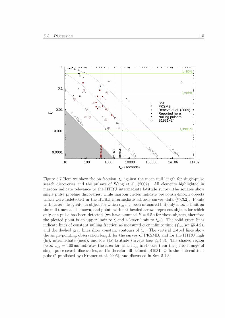
5.4. Discussion 115
ξ
toff (seconds)
ton = 1 s
ton = 10 s
ton = 100 s
f∞=50%
BSBPKSMBDeneva et al. (2009)Reported hereNulling pulsarsB1931+24
0.0001
0.001
0.01
0.1
1
10 100 1000 10000 100000 1e+06 1e+07
PK
SM
B
HT
RU
-lo
HT
RU
-me
d
ton = 100 ms
f∞=95%
f∞=99.9%
Figure 5.7 Here we show the on fraction, ξ, against the mean null length for single-pulsesearch discoveries and the pulsars of Wang et al. (2007). All elements highlighted inmaroon indicate relevance to the HTRU intermediate latitude survey; the squares showsingle pulse pipeline discoveries, while maroon circles indicate previously-known objectswhich were redetected in the HTRU intermediate latitude survey data (§5.3.2). Pointswith arrows designate an object for which ton has been measured but only a lower limit onthe null timescale is known, and points with flat-headed arrows represent objects for whichonly one pulse has been detected (we have assumed P = 8.5 s for these objects, thereforethe plotted point is an upper limit to ξ and a lower limit to toff). The solid green linesindicate lines of constant nulling fraction as measured over infinite time (f∞, see §5.4.2),and the dashed gray lines show constant contours of ton. The vertical dotted lines showthe single-pointing observation length for the survey of PKSMB, and for the HTRU high(hi), intermediate (med), and low (lo) latitude surveys (see §5.4.3). The shaded regionbelow ton = 100ms indicates the area for which ton is shorter than the period range ofsingle-pulse search discoveries, and is therefore ill-defined. B1931+24 is the “intermittentpulsar” published by (Kramer et al. 2006), and discussed in Sec. 5.4.3.
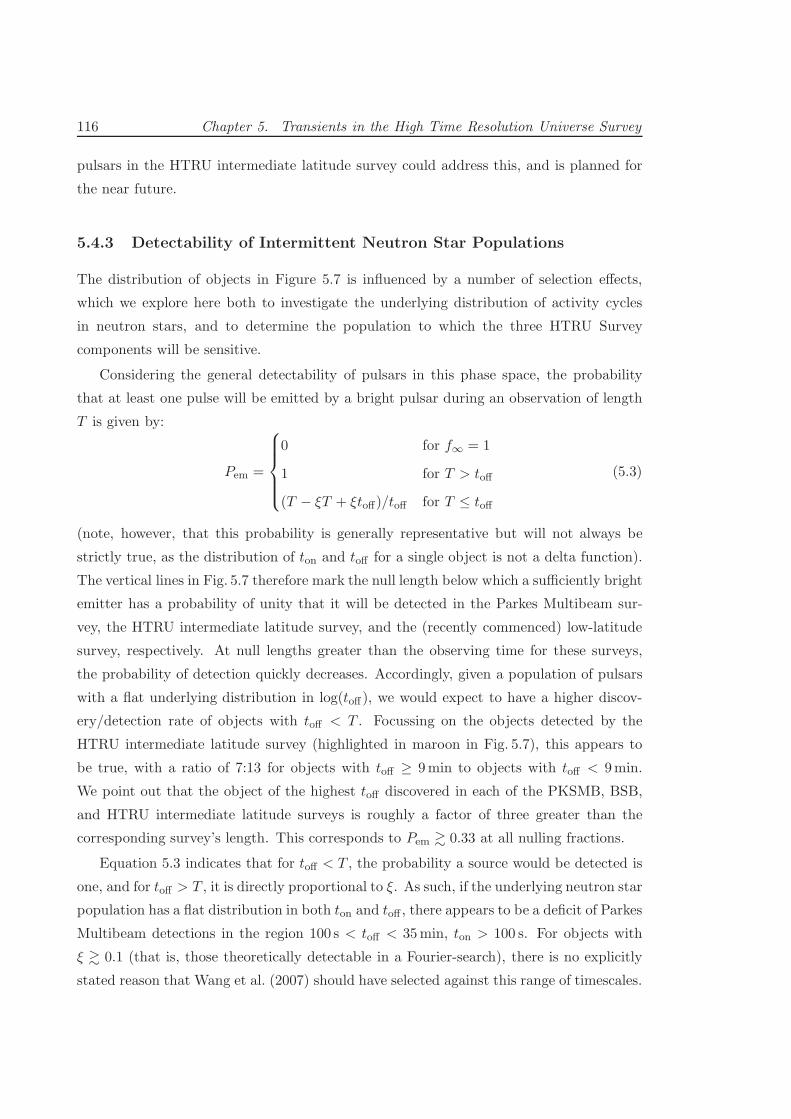
116 Chapter 5. Transients in the High Time Resolution Universe Survey
pulsars in the HTRU intermediate latitude survey could address this, and is planned for
the near future.
5.4.3 Detectability of Intermittent Neutron Star Populations
The distribution of objects in Figure 5.7 is influenced by a number of selection effects,
which we explore here both to investigate the underlying distribution of activity cycles
in neutron stars, and to determine the population to which the three HTRU Survey
components will be sensitive.
Considering the general detectability of pulsars in this phase space, the probability
that at least one pulse will be emitted by a bright pulsar during an observation of length
T is given by:
Pem =
0 for f∞ = 1
1 for T > toff
(T − ξT + ξtoff)/toff for T ≤ toff
(5.3)
(note, however, that this probability is generally representative but will not always be
strictly true, as the distribution of ton and toff for a single object is not a delta function).
The vertical lines in Fig. 5.7 therefore mark the null length below which a sufficiently bright
emitter has a probability of unity that it will be detected in the Parkes Multibeam sur-
vey, the HTRU intermediate latitude survey, and the (recently commenced) low-latitude
survey, respectively. At null lengths greater than the observing time for these surveys,
the probability of detection quickly decreases. Accordingly, given a population of pulsars
with a flat underlying distribution in log(toff ), we would expect to have a higher discov-
ery/detection rate of objects with toff < T . Focussing on the objects detected by the
HTRU intermediate latitude survey (highlighted in maroon in Fig. 5.7), this appears to
be true, with a ratio of 7:13 for objects with toff ≥ 9min to objects with toff < 9min.
We point out that the object of the highest toff discovered in each of the PKSMB, BSB,
and HTRU intermediate latitude surveys is roughly a factor of three greater than the
corresponding survey’s length. This corresponds to Pem & 0.33 at all nulling fractions.
Equation 5.3 indicates that for toff < T , the probability a source would be detected is
one, and for toff > T , it is directly proportional to ξ. As such, if the underlying neutron star
population has a flat distribution in both ton and toff , there appears to be a deficit of Parkes
Multibeam detections in the region 100 s < toff < 35min, ton > 100 s. For objects with
ξ & 0.1 (that is, those theoretically detectable in a Fourier-search), there is no explicitly
stated reason that Wang et al. (2007) should have selected against this range of timescales.
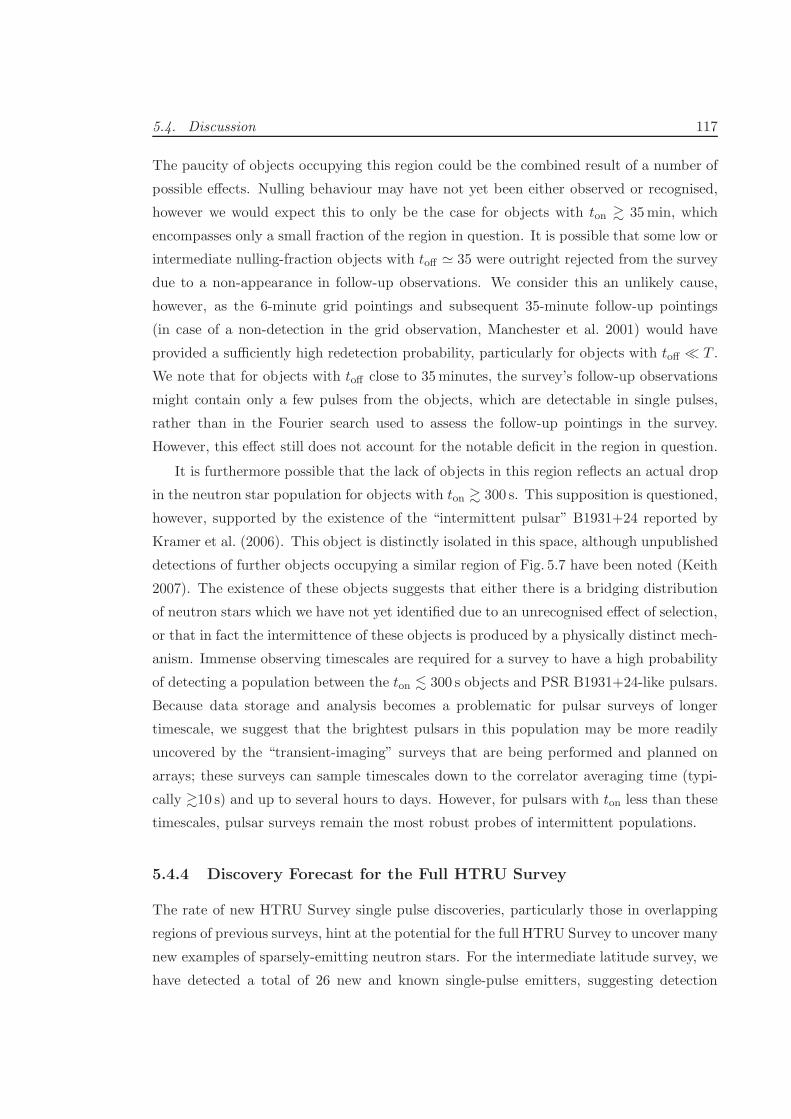
5.4. Discussion 117
The paucity of objects occupying this region could be the combined result of a number of
possible effects. Nulling behaviour may have not yet been either observed or recognised,
however we would expect this to only be the case for objects with ton & 35min, which
encompasses only a small fraction of the region in question. It is possible that some low or
intermediate nulling-fraction objects with toff ≃ 35 were outright rejected from the survey
due to a non-appearance in follow-up observations. We consider this an unlikely cause,
however, as the 6-minute grid pointings and subsequent 35-minute follow-up pointings
(in case of a non-detection in the grid observation, Manchester et al. 2001) would have
provided a sufficiently high redetection probability, particularly for objects with toff ≪ T .
We note that for objects with toff close to 35minutes, the survey’s follow-up observations
might contain only a few pulses from the objects, which are detectable in single pulses,
rather than in the Fourier search used to assess the follow-up pointings in the survey.
However, this effect still does not account for the notable deficit in the region in question.
It is furthermore possible that the lack of objects in this region reflects an actual drop
in the neutron star population for objects with ton & 300 s. This supposition is questioned,
however, supported by the existence of the “intermittent pulsar” B1931+24 reported by
Kramer et al. (2006). This object is distinctly isolated in this space, although unpublished
detections of further objects occupying a similar region of Fig. 5.7 have been noted (Keith
2007). The existence of these objects suggests that either there is a bridging distribution
of neutron stars which we have not yet identified due to an unrecognised effect of selection,
or that in fact the intermittence of these objects is produced by a physically distinct mech-
anism. Immense observing timescales are required for a survey to have a high probability
of detecting a population between the ton . 300 s objects and PSR B1931+24-like pulsars.
Because data storage and analysis becomes a problematic for pulsar surveys of longer
timescale, we suggest that the brightest pulsars in this population may be more readily
uncovered by the “transient-imaging” surveys that are being performed and planned on
arrays; these surveys can sample timescales down to the correlator averaging time (typi-
cally &10 s) and up to several hours to days. However, for pulsars with ton less than these
timescales, pulsar surveys remain the most robust probes of intermittent populations.
5.4.4 Discovery Forecast for the Full HTRU Survey
The rate of new HTRU Survey single pulse discoveries, particularly those in overlapping
regions of previous surveys, hint at the potential for the full HTRU Survey to uncover many
new examples of sparsely-emitting neutron stars. For the intermediate latitude survey, we
have detected a total of 26 new and known single-pulse emitters, suggesting detection
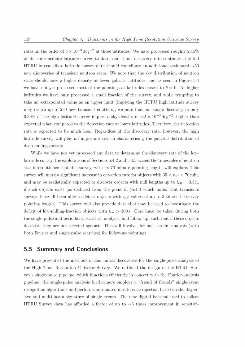
118 Chapter 5. Transients in the High Time Resolution Universe Survey
rates on the order of 3× 10⁻³ deg−2 at these latitudes. We have processed roughly 23.5%
of the intermediate latitude survey to date, and if our discovery rate continues, the full
HTRU intermediate latitude survey data should contribute an additional estimated ∼50
new discoveries of transient neutron stars. We note that the sky distribution of neutron
stars should have a higher density at lower galactic latitudes, and as seen in Figure 5.4
we have not yet processed most of the pointings at latitudes closest to b = 0. At higher
latitudes we have only processed a small fraction of the survey, and while tempting to
take an extrapolated value as an upper limit (implying the HTRU high latitude survey
may return up to 250 new transient emitters), we note that our single discovery in only
0.39% of the high latitude survey implies a sky density of ∼2 × 10⁻³ deg−2, higher than
expected when compared to the detection rate at lower latitudes. Therefore, the detection
rate is expected to be much less. Regardless of the discovery rate, however, the high
latitude survey will play an important role in characterising the galactic distribution of
deep nulling pulsars.
While we have not yet processed any data to determine the discovery rate of the low-
latitude survey, the explorations of Sections 5.4.2 and 5.4.3 accent the timescales of neutron
star intermittence that this survey, with its 70-minute pointing length, will explore. This
survey will mark a significant increase in detection rate for objects with 35 < toff < 70min,
and may be realistically expected to discover objects with null lengths up to toff = 3.5 h,
if such objects exist (as deduced from the point in §5.4.3 which noted that transients
surveys have all been able to detect objects with toff values of up to 3 times the survey
pointing length). This survey will also provide data that may be used to investigate the
deficit of low-nulling-fraction objects with ton > 300 s. Care must be taken during both
the single-pulse and periodicity searches, analysis, and follow-up, such that if these objects
do exist, they are not selected against. This will involve, for one, careful analysis (with
both Fourier and single-pulse searches) for follow-up pointings.
5.5 Summary and Conclusions
We have presented the methods of and initial discoveries for the single-pulse analysis of
the High Time Resolution Universe Survey. We outlined the design of the HTRU Sur-
vey’s single-pulse pipeline, which functions efficiently in concert with the Fourier-analysis
pipeline; the single-pulse analysis furthermore employs a “friend of friends” single-event
recognition algorithms and performs automated interference rejection based on the disper-
sive and multi-beam signature of single events. The new digital backend used to collect
HTRU Survey data has afforded a factor of up to ∼5 times improvement in sensitivi-
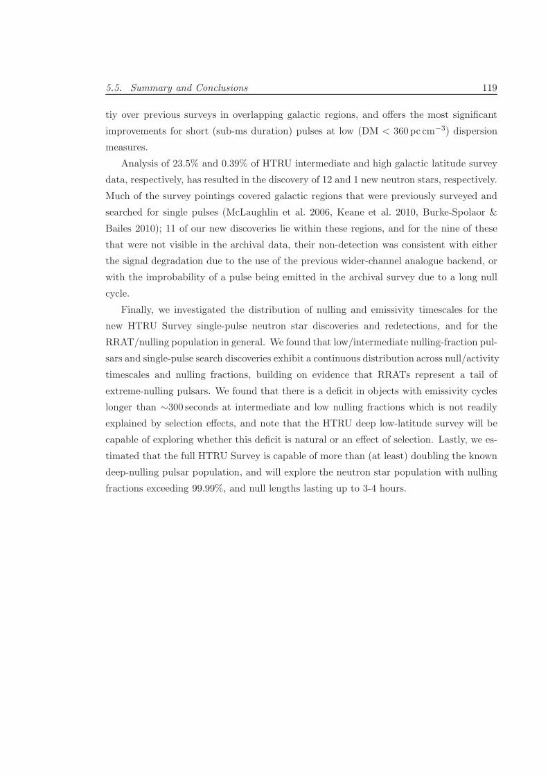
5.5. Summary and Conclusions 119
tiy over previous surveys in overlapping galactic regions, and offers the most significant
improvements for short (sub-ms duration) pulses at low (DM < 360 pc cm−3) dispersion
measures.
Analysis of 23.5% and 0.39% of HTRU intermediate and high galactic latitude survey
data, respectively, has resulted in the discovery of 12 and 1 new neutron stars, respectively.
Much of the survey pointings covered galactic regions that were previously surveyed and
searched for single pulses (McLaughlin et al. 2006, Keane et al. 2010, Burke-Spolaor &
Bailes 2010); 11 of our new discoveries lie within these regions, and for the nine of these
that were not visible in the archival data, their non-detection was consistent with either
the signal degradation due to the use of the previous wider-channel analogue backend, or
with the improbability of a pulse being emitted in the archival survey due to a long null
cycle.
Finally, we investigated the distribution of nulling and emissivity timescales for the
new HTRU Survey single-pulse neutron star discoveries and redetections, and for the
RRAT/nulling population in general. We found that low/intermediate nulling-fraction pul-
sars and single-pulse search discoveries exhibit a continuous distribution across null/activity
timescales and nulling fractions, building on evidence that RRATs represent a tail of
extreme-nulling pulsars. We found that there is a deficit in objects with emissivity cycles
longer than ∼300 seconds at intermediate and low nulling fractions which is not readily
explained by selection effects, and note that the HTRU deep low-latitude survey will be
capable of exploring whether this deficit is natural or an effect of selection. Lastly, we es-
timated that the full HTRU Survey is capable of more than (at least) doubling the known
deep-nulling pulsar population, and will explore the neutron star population with nulling
fractions exceeding 99.99%, and null lengths lasting up to 3-4 hours.


6Terrestrial Impulses that Mimic
Frequency-dependence of Cold Plasma Dispersion
I would rather learn from one bird how to sing
than teach 10000 stars how not to dance.
—e. e. cummings
In this chapter, we report on the serendipitous discovery of “Perytons” in the archival
data search reported in Chapter 4. These surprising discoveries are transient bursts which
show several confounding properties: their frequency sweep mimicks the cold plasma dis-
persion relation typically taken as a sure indication of a celestial origin, but other properties
of the bursts provide solid evidence that their origin is terrestrial. The bursts furthermore
have best-fit dispersion measures which cluster around the DM of the Lorimer Burst
(§1.4.4; Lorimer et al. 2007). This discovery has significant implications for transient
search methods and the suitability of single-dish detectors to make definitive detections
of single impulses. We perform a detailed investigation into the properties and origin of
these signals, and discuss whether the Lorimer Burst and the Perytons have a genesis in
the same phenomenon. While it is not yet clear what is causing the bursts, we propose a
scenario in which the swept-frequency emission could be produced by a lightning-related
plasma phenomenon in Earth’s atmosphere.
6.1 Introduction
As described in §1.4.4, three years ago the “Lorimer Burst” (LB hereafter) was thought to
be the first discovery of a rare, impulsive event of unknown extragalactic origin (Lorimer
et al. 2007). The extragalactic interpretation was based on the swept-frequency nature of
the event, which followed the dispersive delay expected from an extragalactic pulse.
121
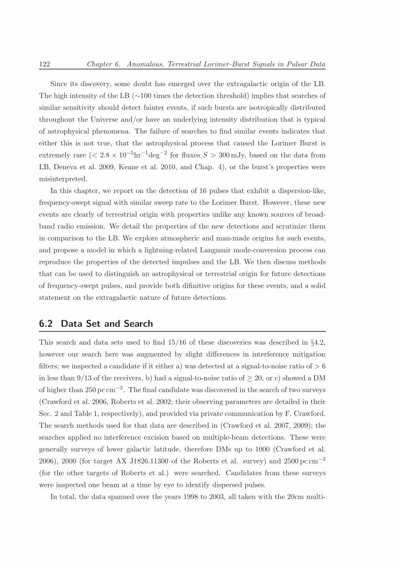
122 Chapter 6. Anomalous, Terrestrial Lorimer-Burst Signals in Pulsar Data
Since its discovery, some doubt has emerged over the extragalactic origin of the LB.
The high intensity of the LB (∼100 times the detection threshold) implies that searches of
similar sensitivity should detect fainter events, if such bursts are isotropically distributed
throughout the Universe and/or have an underlying intensity distribution that is typical
of astrophysical phenomena. The failure of searches to find similar events indicates that
either this is not true, that the astrophysical process that caused the Lorimer Burst is
extremely rare (< 2.8 × 10⁻⁵hr−1deg−2 for fluxes S > 300mJy, based on the data from
LB, Deneva et al. 2009, Keane et al. 2010, and Chap. 4), or the burst’s properties were
misinterpreted.
In this chapter, we report on the detection of 16 pulses that exhibit a dispersion-like,
frequency-swept signal with similar sweep rate to the Lorimer Burst. However, these new
events are clearly of terrestrial origin with properties unlike any known sources of broad-
band radio emission. We detail the properties of the new detections and scrutinize them
in comparison to the LB. We explore atmospheric and man-made origins for such events,
and propose a model in which a lightning-related Langmuir mode-conversion process can
reproduce the properties of the detected impulses and the LB. We then discuss methods
that can be used to distinguish an astrophysical or terrestrial origin for future detections
of frequency-swept pulses, and provide both difinitive origins for these events, and a solid
statement on the extragalactic nature of future detections.
6.2 Data Set and Search
This search and data sets used to find 15/16 of these discoveries was described in §4.2,however our search here was augmented by slight differences in interference mitigation
filters; we inspected a candidate if it either a) was detected at a signal-to-noise ratio of > 6
in less than 9/13 of the receivers, b) had a signal-to-noise ratio of ≥ 20, or c) showed a DM
of higher than 250 pc cm−3. The final candidate was discovered in the search of two surveys
(Crawford et al. 2006, Roberts et al. 2002; their observing parameters are detailed in their
Sec. 2 and Table 1, respectively), and provided via private communication by F. Crawford.
The search methods used for that data are described in (Crawford et al. 2007, 2009); the
searches applied no interference excision based on multiple-beam detections. These were
generally surveys of lower galactic latitude, therefore DMs up to 1000 (Crawford et al.
2006), 2000 (for target AX J1826.11300 of the Roberts et al. survey) and 2500 pc cm−3
(for the other targets of Roberts et al.) were searched. Candidates from these surveys
were inspected one beam at a time by eye to identify dispersed pulses.
In total, the data spanned over the years 1998 to 2003, all taken with the 20cm multi-
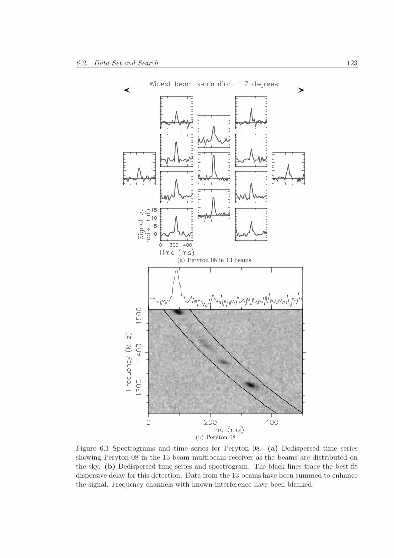
6.2. Data Set and Search 123
(a) Peryton 08 in 13 beams
(b) Peryton 08
Figure 6.1 Spectrograms and time series for Peryton 08. (a) Dedispersed time seriesshowing Peryton 08 in the 13-beam multibeam receiver as the beams are distributed onthe sky. (b) Dedispersed time series and spectrogram. The black lines trace the best-fitdispersive delay for this detection. Data from the 13 beams have been summed to enhancethe signal. Frequency channels with known interference have been blanked.
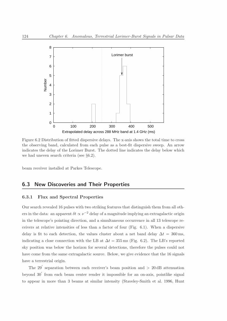
124 Chapter 6. Anomalous, Terrestrial Lorimer-Burst Signals in Pulsar Data
0
1
2
3
4
5
6
7
8
0 100 200 300 400 500
Num
ber
Extrapolated delay across 288 MHz band at 1.4 GHz (ms)
Lorimer burst
Figure 6.2 Distribution of fitted dispersive delays. The x-axis shows the total time to crossthe observing band, calculated from each pulse as a best-fit dispersive sweep. An arrowindicates the delay of the Lorimer Burst. The dotted line indicates the delay below whichwe had uneven search criteria (see §6.2).
beam receiver installed at Parkes Telescope.
6.3 New Discoveries and Their Properties
6.3.1 Flux and Spectral Properties
Our search revealed 16 pulses with two striking features that distinguish them from all oth-
ers in the data: an apparent δt ∝ ν−2 delay of a magnitude implying an extragalactic origin
in the telescope’s pointing direction, and a simultaneous occurrence in all 13 telescope re-
ceivers at relative intensities of less than a factor of four (Fig. 6.1). When a dispersive
delay is fit to each detection, the values cluster about a net band delay ∆t = 360ms,
indicating a close connection with the LB at ∆t = 355ms (Fig. 6.2). The LB’s reported
sky position was below the horizon for several detections, therefore the pulses could not
have come from the same extragalactic source. Below, we give evidence that the 16 signals
have a terrestrial origin.
The 29′separation between each receiver’s beam position and > 20 dB attenuation
beyond 30′from each beam center render it impossible for an on-axis, pointlike signal
to appear in more than 3 beams at similar intensity (Staveley-Smith et al. 1996, Hunt
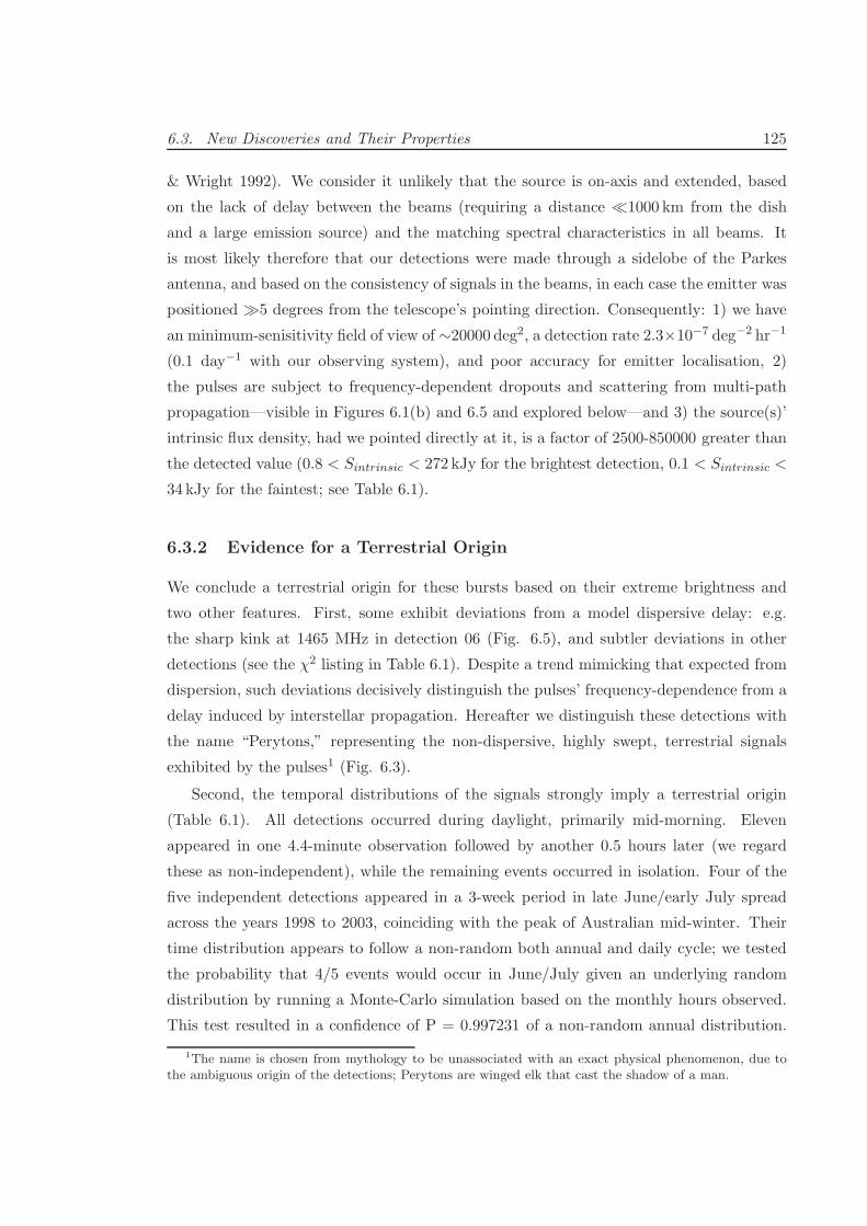
6.3. New Discoveries and Their Properties 125
& Wright 1992). We consider it unlikely that the source is on-axis and extended, based
on the lack of delay between the beams (requiring a distance ≪1000 km from the dish
and a large emission source) and the matching spectral characteristics in all beams. It
is most likely therefore that our detections were made through a sidelobe of the Parkes
antenna, and based on the consistency of signals in the beams, in each case the emitter was
positioned ≫5 degrees from the telescope’s pointing direction. Consequently: 1) we have
an minimum-senisitivity field of view of ∼20000 deg2, a detection rate 2.3×10⁻⁷ deg−2 hr−1
(0.1 day−1 with our observing system), and poor accuracy for emitter localisation, 2)
the pulses are subject to frequency-dependent dropouts and scattering from multi-path
propagation—visible in Figures 6.1(b) and 6.5 and explored below—and 3) the source(s)’
intrinsic flux density, had we pointed directly at it, is a factor of 2500-850000 greater than
the detected value (0.8 < Sintrinsic < 272 kJy for the brightest detection, 0.1 < Sintrinsic <
34 kJy for the faintest; see Table 6.1).
6.3.2 Evidence for a Terrestrial Origin
We conclude a terrestrial origin for these bursts based on their extreme brightness and
two other features. First, some exhibit deviations from a model dispersive delay: e.g.
the sharp kink at 1465 MHz in detection 06 (Fig. 6.5), and subtler deviations in other
detections (see the χ2 listing in Table 6.1). Despite a trend mimicking that expected from
dispersion, such deviations decisively distinguish the pulses’ frequency-dependence from a
delay induced by interstellar propagation. Hereafter we distinguish these detections with
the name “Perytons,” representing the non-dispersive, highly swept, terrestrial signals
exhibited by the pulses1 (Fig. 6.3).
Second, the temporal distributions of the signals strongly imply a terrestrial origin
(Table 6.1). All detections occurred during daylight, primarily mid-morning. Eleven
appeared in one 4.4-minute observation followed by another 0.5 hours later (we regard
these as non-independent), while the remaining events occurred in isolation. Four of the
five independent detections appeared in a 3-week period in late June/early July spread
across the years 1998 to 2003, coinciding with the peak of Australian mid-winter. Their
time distribution appears to follow a non-random both annual and daily cycle; we tested
the probability that 4/5 events would occur in June/July given an underlying random
distribution by running a Monte-Carlo simulation based on the monthly hours observed.
This test resulted in a confidence of P = 0.997231 of a non-random annual distribution.
1The name is chosen from mythology to be unassociated with an exact physical phenomenon, due tothe ambiguous origin of the detections; Perytons are winged elk that cast the shadow of a man.
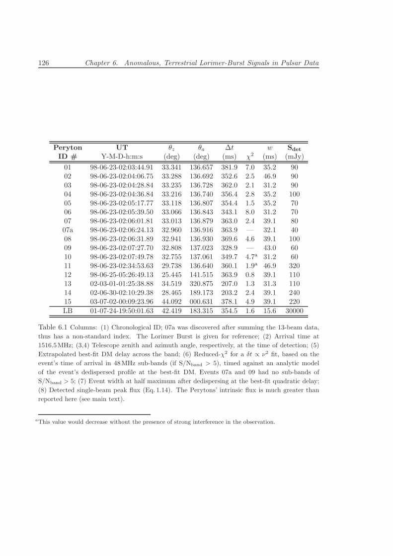
126 Chapter 6. Anomalous, Terrestrial Lorimer-Burst Signals in Pulsar Data
Peryton UT θz θa ∆t w Sdet
ID # Y-M-D-h:m:s (deg) (deg) (ms) χ2 (ms) (mJy)
01 98-06-23-02:03:44.91 33.341 136.657 381.9 7.0 35.2 9002 98-06-23-02:04:06.75 33.288 136.692 352.6 2.5 46.9 9003 98-06-23-02:04:28.84 33.235 136.728 362.0 2.1 31.2 9004 98-06-23-02:04:36.84 33.216 136.740 356.4 2.8 35.2 10005 98-06-23-02:05:17.77 33.118 136.807 354.4 1.5 35.2 7006 98-06-23-02:05:39.50 33.066 136.843 343.1 8.0 31.2 7007 98-06-23-02:06:01.81 33.013 136.879 363.0 2.4 39.1 8007a 98-06-23-02:06:24.13 32.960 136.916 363.9 — 32.1 4008 98-06-23-02:06:31.89 32.941 136.930 369.6 4.6 39.1 10009 98-06-23-02:07:27.70 32.808 137.023 328.9 — 43.0 6010 98-06-23-02:07:49.78 32.755 137.061 349.7 4.7a 31.2 6011 98-06-23-02:34:53.63 29.738 136.640 360.1 1.9a 46.9 32012 98-06-25-05:26:49.13 25.445 141.515 363.9 0.8 39.1 11013 02-03-01-01:25:38.88 34.519 320.875 207.0 1.3 31.3 11014 02-06-30-02:10:29.38 28.465 189.173 203.2 2.4 39.1 24015 03-07-02-00:09:23.96 44.092 000.631 378.1 4.9 39.1 220
LB 01-07-24-19:50:01.63 42.419 183.315 354.5 1.6 15.6 30000
Table 6.1 Columns: (1) Chronological ID; 07a was discovered after summing the 13-beam data,
thus has a non-standard index. The Lorimer Burst is given for reference; (2) Arrival time at
1516.5MHz; (3,4) Telescope zenith and azimuth angle, respectively, at the time of detection; (5)
Extrapolated best-fit DM delay across the band; (6) Reduced-χ2 for a δt ∝ ν2 fit, based on the
event’s time of arrival in 48MHz sub-bands (if S/Nband > 5), timed against an analytic model
of the event’s dedispersed profile at the best-fit DM. Events 07a and 09 had no sub-bands of
S/Nband > 5; (7) Event width at half maximum after dedispersing at the best-fit quadratic delay;
(8) Detected single-beam peak flux (Eq. 1.14). The Perytons’ intrinsic flux is much greater than
reported here (see main text).
aThis value would decrease without the presence of strong interference in the observation.
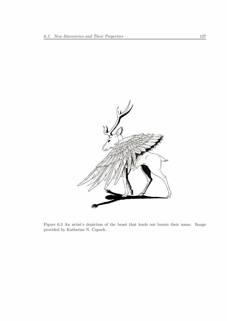
6.3. New Discoveries and Their Properties 127
Figure 6.3 An artist’s depiction of the beast that lends our bursts their name. Imageprovided by Katherine N. Capach.
128 Chapter 6. Anomalous, Terrestrial Lorimer-Burst Signals in Pulsar Data
A similar test based on the time of day distribution of observations and detections gave
a probability of P = 0.999046 that 4/5 events would occur in the UT range 0–3. These
cycles are strongly suggestive of either a climate/weather-related effect, or a man-made
origin for the emission.
6.4 Discussion
6.4.1 Signal Origins
It is unprecedented for non-astrophysical emission to exhibit such drastic frequency-
dependent delays in the 1 GHz band. Given the daytime occurrence of the Perytons,
we first explored the possibility of the signals as man-made. The continuous emission
across the legally protected 1400-1427 MHz band suggest that the signal is not intention-
ally transmitted (although do not rule out the possibility); additionally, the combination of
a lack of regular periodicity, the broad pulse widths (30-50 ms), and broad-band emission
preclude a radar origin. Man-made emission that is unintentionally transmitted arises of-
ten from on-site electronic hardware failure. This does not appear to be the source of this
emission, however, based primarily on the amplitude modulation seen in all the detections.
These amplitude-modulated temporal or frequency structures show conformity across the
spectrum in all 13 beams for each burst. Assuming the modulation is attributable to
multi-path propagation effects (that these detections will necessarily show, as noted in
§6.3 above), the incoming wavefront must not decorrelate over the physical size of the
telescope’s feed horns (1 meter), to allow the similarity of the modulation structures in
all 13 beams. The diffractive scale (s0), therefore, must likewise be ≥ 1m. Taking the
characteristic bandwidth of the modulation structure in all pulses to be ∆f ∼ 10MHz),
and based on the center frequency f = 1374MHz, we place a lower limit on the distance
to the object(s) and scatterer(s) of 2π(s0f)2/c∆f > 4 km. This suggests that we have de-
tected emission from the horizon—well off-site from the telescope grounds—and provides
the strongest argument against on-site hardware failure as the source. The quasi-annual
cycle and the spectral complexity with a 6-year persistence of the signal also argue against
local hardware failures as the emission’s origin.
While we cannot rule out an unknown satellite-based origin for the signals, it is per-
tinent to consider the possibility that the Perytons were caused by a natural terrestrial
source. Given the inconsistencies of the signals with man-made origins, we did explore
this possibility, considering processes that can produce non-dispersive, swept emission
with sweep rates of ∼1GHz/s. The emission requires a process of finite-bandwidth
6.4. Discussion 129
(∆f < 25MHz) signal to progressively change in its center frequency, for instance cy-
clotron emission in a time-varying magnetic field or the progressive incitement of plasma
oscillations in regions of differing plasma density.
The latter of these processes occurs in type III solar bursts (e. g. Loughhead et al.
1957b), in which we find a well-suited explanation for our bursts in a Langmuir wave mode-
conversion mechanism, in which a flare propagates through a plasma of changing density,
inducing electromagnetic waves at the plasma frequency (or its second harmonic) and
resulting in a flare swept with attributes characterised by the velocity of the flare and the
shape of the density gradient along the flare propagation path. Such emission, for instance,
arises from the type III solar bursts at sub-GHz frequencies (Loughhead et al. 1957b) noted
in §1.4.3. Emission via this mechanism in our observing band requires electron number
densities of order 1016 m−3. Such densities are transiently reached by ionised channels
that accompany electrical storm phenomena, ranging >1010 m−3 for upper-atmospheric
”red sprites” (Dowden et al. 2001), up to 1023 m−3 for cloud-to-ground lightning (Rakov &
Uman 2003). A super-ionisation event of this magnitude would be required for terrestrial,
swept plasma-oscillation emission in our band.
6.4.2 Investigation of Atmospheric Plasma Emission Origins
We investigated the suitability of an atmospheric Langmuir wave emission model to explain
our impulses by considering the simple case of propagation vertical, lightning-induced
plasma channel at 100% atmospheric ionisation.
An atmospheric plasma emitting at a radio frequency f (i. e. an electron plasma fre-
quency ωp = 2πf), must have a sufficiently high level of ionization to have a free electron
density, ne, obeying f =√
nee2/mǫ0/2π. Emission swept through our observing band,
from f1 = 1516.5 MHz to f2 = 1228.5 MHz, requires ne1 = 2.853 × 10¹⁶/m3 for f1, and
ne2 = 1.872×10¹⁶/m3 for f2, or one fourth of these values if the detected emission is a sec-
ond emission harmonic (2ωp). The electron density cannot exceed the electrons available
in the ambient atmosphere, therefore the height of the emission is limited to approximately
the height below which the atmospheric atomic number density, natm, is equal to ne1. Us-
ing the altitude-dependent atmospheric density from the “US Standard Atmosphere 1976”
(USSA) atmospheric model2, in a complete breakdown of the atmosphere we estimate the
maximum available electron density at altitude h to be ne(h) ≃ natm(h) = ρ(h)NA/M(h),
where NA is the Avogadro constant, and M(h) and ρ(h) are the mean atomic weight and
2The U. S. Standard Atmosphere. NASA, Washington, D. C. (1976), available fromhttp://modelweb.gsfc.nasa.gov/atmos/us standard.html
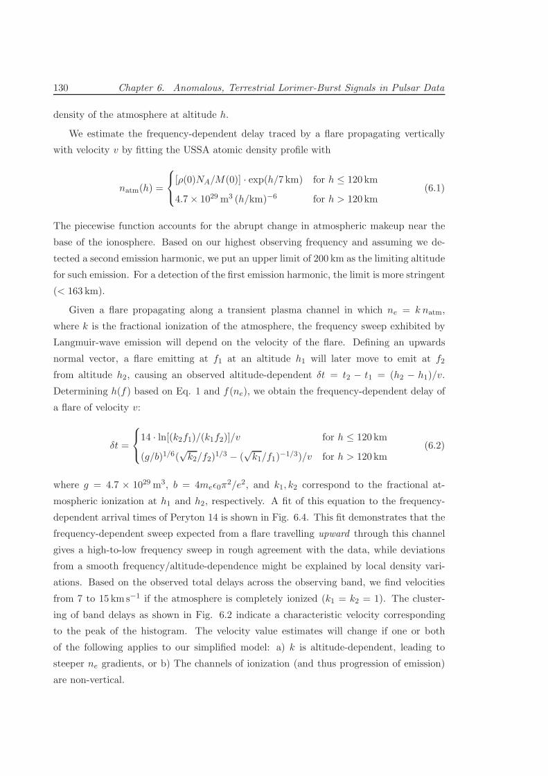
130 Chapter 6. Anomalous, Terrestrial Lorimer-Burst Signals in Pulsar Data
density of the atmosphere at altitude h.
We estimate the frequency-dependent delay traced by a flare propagating vertically
with velocity v by fitting the USSA atomic density profile with
natm(h) =
[ρ(0)NA/M(0)] · exp(h/7 km) for h ≤ 120 km
4.7× 1029 m3 (h/km)−6 for h > 120 km(6.1)
The piecewise function accounts for the abrupt change in atmospheric makeup near the
base of the ionosphere. Based on our highest observing frequency and assuming we de-
tected a second emission harmonic, we put an upper limit of 200 km as the limiting altitude
for such emission. For a detection of the first emission harmonic, the limit is more stringent
(< 163 km).
Given a flare propagating along a transient plasma channel in which ne = k natm,
where k is the fractional ionization of the atmosphere, the frequency sweep exhibited by
Langmuir-wave emission will depend on the velocity of the flare. Defining an upwards
normal vector, a flare emitting at f1 at an altitude h1 will later move to emit at f2
from altitude h2, causing an observed altitude-dependent δt = t2 − t1 = (h2 − h1)/v.
Determining h(f) based on Eq. 1 and f(ne), we obtain the frequency-dependent delay of
a flare of velocity v:
δt =
14 · ln[(k2f1)/(k1f2)]/v for h ≤ 120 km
(g/b)1/6(√k2/f2)
1/3 − (√k1/f1)
−1/3)/v for h > 120 km(6.2)
where g = 4.7 × 1029 m3, b = 4meǫ0π2/e2, and k1, k2 correspond to the fractional at-
mospheric ionization at h1 and h2, respectively. A fit of this equation to the frequency-
dependent arrival times of Peryton 14 is shown in Fig. 6.4. This fit demonstrates that the
frequency-dependent sweep expected from a flare travelling upward through this channel
gives a high-to-low frequency sweep in rough agreement with the data, while deviations
from a smooth frequency/altitude-dependence might be explained by local density vari-
ations. Based on the observed total delays across the observing band, we find velocities
from 7 to 15 km s−1 if the atmosphere is completely ionized (k1 = k2 = 1). The cluster-
ing of band delays as shown in Fig. 6.2 indicate a characteristic velocity corresponding
to the peak of the histogram. The velocity value estimates will change if one or both
of the following applies to our simplified model: a) k is altitude-dependent, leading to
steeper ne gradients, or b) The channels of ionization (and thus progression of emission)
are non-vertical.
6.4. Discussion 131
0
0.05
0.1
0.15
0.2
Rel
ativ
e ar
rival
tim
e (s
econ
ds)
Dispersive delayVertical atmospheric propagationBurst 14 band-dependent arrival times
-0.010
0.01
-0.010
0.01
1250 1300 1350 1400 1450 1500
Diff
eren
ce
Frequency (MHz)
Figure 6.4 Frequency-dependent arrival time of Peryton 14 and models. The upper panelshows the arrival time (points and errors) in 24-MHz-averaged bands relative to the 1512MHz arrival. The best-fit dispersive delay is plotted in black and the Langmuir-emissiondelay expected from a simple atmospheric model is plotted in gray. The lower panelsshow the residual arrivals after subtraction of the models. To avoid preselection towardsa dispersion sweep, this timing analysis used sub-bands that were not dedispersed beforeaveraging, and employed the brightest sub-band as a timing template.
132 Chapter 6. Anomalous, Terrestrial Lorimer-Burst Signals in Pulsar Data
If this mechanism is indeed the cause of the Perytons, the upward propagation, high
plasma density, and >350ms ion persistence time necessary to produce our signal suggest
an association with upper-atmospheric storm phenomena such as the aforementioned red
sprites, or gigantic jets (Sentman et al. 1995, Wescott et al. 1995, Su et al. 2003).
6.4.3 Weather-related Effects: Ducting, Annual Cycles, and Storm Ac-
tivity
While Australian storm rates do not peak in June/July, this period coincides with Aus-
tralian mid-winter. On the days of four independent detections for which data was avail-
able, the online Parkes weather archives3 indicate moderate rainfall on three, despite a
generally dry climate. This evidence leads us to suggest that such weather conditions
and the atmospheric state at mid-morning in winter provide an elevated likelihood for
high-frequency tropospheric ducting modes to form (Hall 1979, Union 1996), allowing the
detection of distant emission not usually detectable by the telescope. Elevated detec-
tions during mid-winter mornings of transmitters known to be beyond the Parkes horizon
provide strong support for this hypothesis (provided via private communication by J.
Reynolds). Australian lightning activity was not elevated to a statistically significant level
for the days of detection 4, however we do find cloud-to-ground lightning strikes indicating
electrically active oceanic storms occurring within 6 minutes of each event, at distances
less than 2000 km from the telescope. These coastal storms represent possible origins for
Langmuir emission in the presence of a tropospheric duct.
6.5 A Closer Look at the Lorimer Burst
Returning now to the event that motivated this work, we would like to expand on the
relationship of the LB to the Perytons. Whether the LB has the same origin as our detec-
tions remains a somewhat open question, these signals add serious doubt its extragalactic
interpretation. Several qualitative differences between the LB and the Perytons warrant
examination. The LB was clearly detected in only 3 of the 13 beams (6, 7, and D). It is
marginally detectable in other beams, most prominently in beams 5 and C, and apparent
in a stacked time series of the remaining beams. Based on observations of the inner side-
lobe pattern of the multibeam by L. Staveley-Smith (private communication), we find a
position of the LB (consistent with both the relative detected flux levels in beams 6, 7, C,
3“Parkes Observatory Weather Statistics” (accessed 2009):http://www.parkes.atnf.csiro.au/cgi-bin/monitoring/wstats.cgi
4Queried in 2009 through the “Lightning Incident Archive Search”: http://www.gpats.com.au
6.5. A Closer Look at the Lorimer Burst 133
D, and the non-detections in the other beams) at R.A. 19.44 ± 0.08, decl. −75.17 ± 0.08.
That is, the relative signal levels of the LB conform to those expected from a boresight
signal, in agreement with the same conclusion of Lorimer et al. (2007). Therefore, if the
LB is a Peryton, it appears to be the only detection for which the telescope was pointed
directly at the emitter. Consequently, although the LB did not exhibit the same deep
spectral signal modulation as the Perytons, these differences are well accounted for by the
multi-path effects which we interpreted to arise from the horizon-based sidelobe detections
of the Perytons (§6.4.1).
Note that because the beam and sidelobe shapes of the multibeam scale with frequency,
the offset of the burst from the center of beam 6 will induce a spectral steepening of
the source, causing the intrinsic spectrum to be flatter than that originally reported by
Lorimer et al. (2007) by αintrinsic = αobserved−αinduced (where S ∝ να). The Staveley-Smith
measurements were made at two frequencies, allowing quantification of this effect. Within
the error of our positional measurements, the induced spectral index is αinduced = −1+0.9−2.0.
Therefore, at our estimate of position, the intrinsic spectral index is αintrinsic = −2.5−0.6,
where we have measured the observed spectrum in beam 6 to follow αobs = −2.6.
If the LB was caused by a sky-based object (e. g. an aircraft, satellite, or the Langmuir
wave emission proposed above), we might expect to detect some movement of the LB
across the field of the multibeam. We can limit the movement by noting that because
the signal saturated beam 6 for the entirety of its sweep, it is clear that the emitter
did not travel sufficiently far to cross a null in the sidelobes of beam 6. Therefore, we
limit any movement of the emitter to < 35 arcminutes, corresponding to a distance of
d = 0.015h/sin(θ), where h is the emitter’s altitude and θ is the angle between the
telescope’s line of sight and the LB’s velocity vector. At 12 km (a typical aircraft/cloud
height), this corresponds to a distance and velocity of 180m and 500m/s, respectively,
if the LB is moving perpendicularly to the line of sight. This does not put rigorous
limits on aircraft movement, however does place bounds on the quantitative model in
6.4.2, requiring either non-vertical movement of the emitter, or the condition k2 < k1, for
the model to hold for the LB. If an accurate measurement of the inner sidelobes of the
mutlibeam receiver and their frequency-dependence were available, it may be possible to
place a more stringent limit on (or provide a measurement of) movements of the LB.
One major point of discrepancy remains between the LB and the Perytons: that
their widths disagree by a factor of ∼2 (which cannot be accounted for by multi-path
scatter broadening), and we do not observe a frequency-dependent pulse width evolution
in the Perytons. However, we are hindered in measuring frequency-dependent evolution
134 Chapter 6. Anomalous, Terrestrial Lorimer-Burst Signals in Pulsar Data
in the Perytons because of their modulated signal. While the difference in pulse width
lends weak remaining support for a divide between the LB and the Perytons, with our
current measurements it cannot be ruled out that there may be an underlying pulse width
distribution, and/or a dependence on width with an event’s intrinsic flux; likewise we
cannot state whether frequency dependence of pulse width is intrinsic to the phenomenon
causing all the events.
6.6 Conclusions: Implications for Current and Future Transient
Experiments
Regardless of the physical origin of the Perytons or the LB, the results of this study illus-
trate the limitations of single-dish radio burst detection experiments to provide conclusive
evidence for the origins of one-off bursts; dispersive delays can provide the only evidence
for an astrophysical nature on single-detector detections, while multi-detector (i. e. array)
experiments can provide wavefront measurement and localization for localized pulses, or
can assure non-correlation of local signals between widely-spaced array elements. Array
experiments are necessary to provide a conclusive origin for further detections of the class
of pulses presented here, as well as for any future experiments that aim to detect and use
extragalactic pulses in scientific studies. Two such experiments are currently underway at
the Giant Metre Wave and Very Long Baseline Array telescopes, and will be possible with
the Square Kilometre Array and its pathfinder experiments. Single-dish measurements
can improve our understanding of these events by providing polarisation measurements,
and further detections for world, temporal, and delay-distribution statistics.
If our detections do originate from a natural terrestrial process with intrinsic flux
≫100 Jy, detections are expected at other observatories with similar capabilities to Parkes
and ongoing pulsar and transient observations (e.g. Arecibo Observatory, Green Bank
and Effelsberg Telescopes). It is an undeniable curiosity that no Perytons have yet been
identified at radio observatories where such searches have been performed (e. g. Amy et al.
1989, Nice 1999, Deneva et al. 2009). However, it is possible that they have not occurred
during observations (one should occur per∼215 h of data on a telescope with similar system
temperature and sidelobe suppression levels to Parkes, if the event rate is the same at other
sites), that interference rejection algorithms based on the appearance of signals in multiple
beams have removed the signals, that the searches were at frequencies where Perytons are
not emitted, and/or that the experiments were not sensitive to pulses of 30-50ms width.
As multi-detector coincidence filters will strongly preclude the detection of Perytons, the
6.6. Conclusions 135
strength of such rejection filters to limit local interference of any form is clear; however
it is likewise clear that the filters would need to be relaxed to maximize an observatory’s
capability to detect and identify the origin of these remarkable signals. Additionally, we
believe that it was the human inspection of the spectrogram data and multi-beam time
series for each candidate (described in §6.2) that were the main contributors to the first
recognition of the peculiar nature of the Perytons—the simultaneous occurrence of clear,
seemingly dispersed emission and multiple-beam detection—and that encouraged us to
scrutinize these events more closely instead of disregarding them as spurious detections.
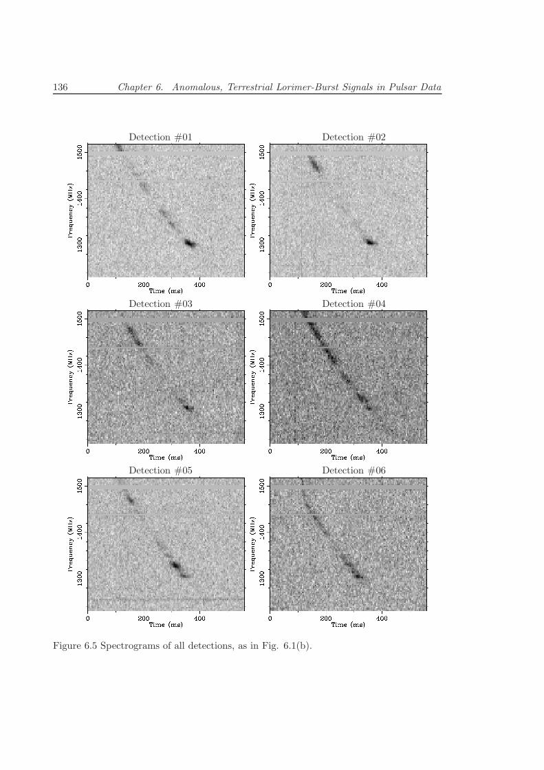
136 Chapter 6. Anomalous, Terrestrial Lorimer-Burst Signals in Pulsar Data
Detection #01 Detection #02
Detection #03 Detection #04
Detection #05 Detection #06
Figure 6.5 Spectrograms of all detections, as in Fig. 6.1(b).
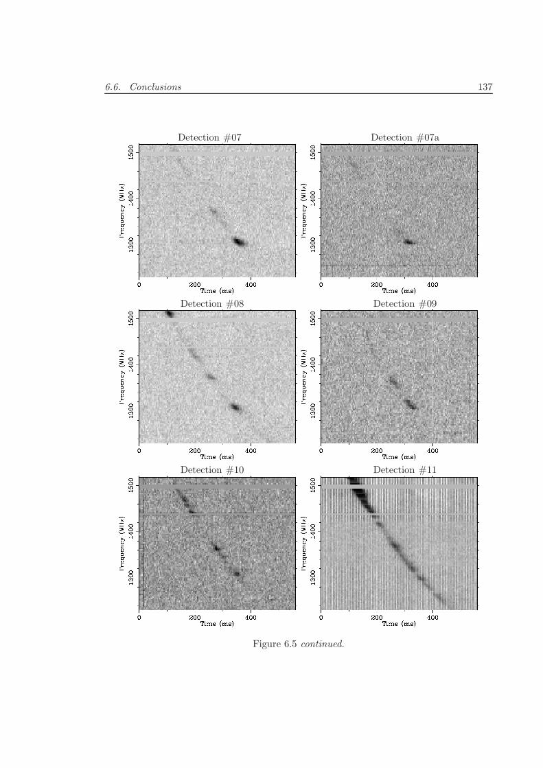
6.6. Conclusions 137
Detection #07 Detection #07a
Detection #08 Detection #09
Detection #10 Detection #11
Figure 6.5 continued.
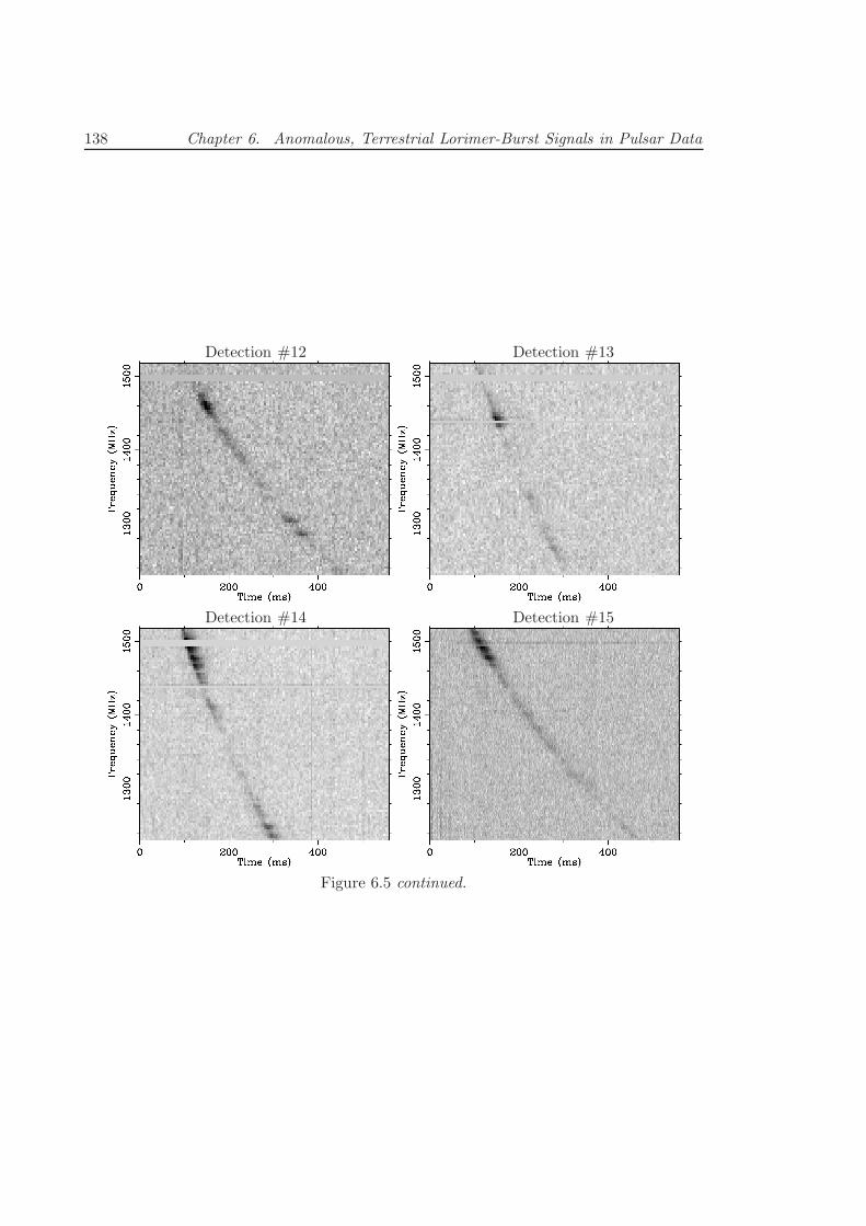
138 Chapter 6. Anomalous, Terrestrial Lorimer-Burst Signals in Pulsar Data
Detection #12 Detection #13
Detection #14 Detection #15
Figure 6.5 continued.
7Conclusions and Future Directions
7.1 Conclusions and Major Findings of this Thesis
Motivated by the broad-reaching scientific endeavours encompassed by “pulsar astron-
omy,” this research has advanced the knowledge of various astronomical and physical
topics. In particular:
Gravitational Wave Astronomy: In Chapter 2, we examined the possibility of detect-
ing supermassive black hole binary systems through both gravitational wave and electro-
magnetic signatures. We concluded that two electromagnetic tracers of black holes—high
resolution radio spectral mapping and emission lines from the gas surrounding an active
galactic nucleus—have significant overlap in the masses, orbital periods, and distances of
systems to which pulsar timing is theoretically sensitive to their gravitational radiation.
Blind searches for electromagnetic signatures of binary supermassive black holes will be
limited by the number of electromagnetically-emitting cores in the Universe, but discover-
ies should be possible given a rigorous search of a large sample. The identification of binary
systems emitting gravitational waves in the pulsar timing band will raise the sensitivity of
pulsar timing arrays manyfold and may enable the first direct detection of gravitational
wave emission as pulsar timing improves its sensitivity to gravitational waves from these
objects.
Galaxy merger dynamics: Exploiting one of the search methods of Chap. 2, we em-
barked on a search for supermassive binary systems in archival radio data. The possibility
that supermassive binaries might “stall” at small orbital separations has been an ongoing
issue in post-merger dynamical theory that—if more than theoretical fancy—would have
detrimental implications for detecting gravitational radiation with pulsar timing arrays.
Our search resulted in the first observational evidence against this possibility. The data
indicate an efficient inspiral evolution to within the purported stalling radius, however
139
140 Chapter 7. Conclusions and Future Directions
with a timescale of sufficient length that it may produce a non-negligible effect in predic-
tive models for the amplitude of the gravitational wave background in the pulsar timing
band.
Radio transient searches and search methods: We have developed a new inspection
and anti-coincidence search methodology that uses the methods outlined by Cordes &
McLaughlin (2003), and expands on them by employing several novel techniques: 1) iden-
tification of discrete events and reconstruction of their observed properties, 2) automated
dispersion measure- and multi-detector-based interference excision, and 3) candidate in-
spection of data for single events. These techniques have enabled improved discrimination
between interference and low-dispersion (i. e. very nearby, or high galactic latitude) im-
pulses, as evidenced by the low dispersion measure of many of our discoveries (19 below
DM = 88pc cm−3, with the lowest having a dispersion measure of DM = 9.2 pc cm−3)
as compared to the original search that discovered “rotating radio transients” (RRATs
McLaughlin et al. 2006; all above DM > 88 pc cm−3). The software to perform these
searches is highly portable and has been made available to the public domain for use at
other radio telescope facilities.
Neutron star discoveries: Utilising the search methods and software developed in
this thesis, we have contributed the discovery of 27 neutron stars to the known pulsar
population. Approximately 90% of the new discoveries represent a significant contribution
to extreme nulling pulsars, of which previously .50 were known. Of particular interest
are several objects. PSR J0941–39 appears part-time as a low-fraction nulling pulsar and
otherwise appears as a sparsely-emitting “rotating radio transient,” and likely represents
an evolutionary transition between two states of emission. PSR J0410–3107 holds several
“records” for extreme nulling pulsars/RRATs, being the closest known RRAT to Earth,
that of the highest galactic latitude, and lowest dispersion measure (9.2 pc cm−3; this DM
is also lower than 98.9% of known radio pulsars).
Insights into sparsely emitting neutron stars: The new discoveries of sparsely-
emitting neutron stars have revealed further insight into the nature of the pulsar-related
phenomenon “rotating radio transients.” We have concluded that some of the objects
classified as RRATs do appear to be genuinely intermittent (rather than faint/distant
pulsars with long-tailed pulse energy distributions). Furthermore, the RRAT population
appears to have both a galactic distribution and a duty cycle distribution very similar to
average pulsars. These insights, as well as the pulsar J0941–39’s bimodal emission states,
support the suggestion that RRATs are more likely to be extreme examples of nulling
pulsars, where the length of their “on” emission is less than one rotational period. The
7.2. Future directions 141
analysis of emission and null timescales for transient emitters suggests that rather than
RRATs, the “intermittent pulsars” like PSR B1931+24 (Kramer et al. 2006) appear to
represent a distinct class of transient neutron star phenomena.
The dynamic radio sky: We have made several new neutron star discoveries in the
High Time Resolution Universe Survey in regions of overlap with previous pulsar and
transients surveys. These new discoveries are a testimony to the dynamic nature of the
transient radio sky, and the analysis in Chapter 5 has indicated that surveys of long
pointing duration, e. g. the HTRU low-latitude survey, will be capable of both discovering
pulsars with nulling fractions greater than 99.99% (that is, pulsing only once per 3-4
hours), and will explore what appears to be a deficit of neutron stars which are active for
timescales above 300 s but have nulling lengths greater than ∼100 s.
Terrestrial and extragalactic radio transient phenomena: We discovered 16 im-
pulses (“Perytons”) of .50ms duration whose swept-frequency signal closely mimics, how-
ever is not caused by, cold plasma dispersion. The pulses are caused by an unknown
phenomenon of terrestrial or Earth-local origin. Their existence has several consequences:
1) They draw significant doubt on the origin of the only reported detection of an extra-
galactic radio impulse (Lorimer et al. 2007); 2) Their similarity to cold plasma dispersion
severely limits the use of many pulsar surveys to characterise extragalactic pulse popu-
lations. Specifically, the single-detector experiments in current common use for pulsar
searches have insufficient capability to definitively distinguish one-off terrestrial pulses
from those of celestial origin; 3) There is an unidentified terrestrial phenomenon which
exhibits strongly frequency-swept emission. We have explored a possible atmospheric
plasma origin with a model that can reproduce most of the properties of the pulses. If
this is the source, it may imply possible ties to the upper-atmospheric Transient Lumi-
nous Event phenomena (e. g. Su et al. 2003) that on occasion accompany electrical storm
activity. However, further exploration and further detections are undoubtedly required to
determine the actual pulse origins.
7.2 Future directions
Pulsar astronomy remains an ambitious and far-reaching scientific field. This thesis has
contributed to two areas, radio transient and gravitational wave astronomy, as their own
rising and highly dynamic fields of research. The work in this thesis has opened a base of
new questions that may be answered using both current radio telescopes and the upcoming
generation of telescopes such as the Square Kilometre Array and its pathfinders. Here we
142 Chapter 7. Conclusions and Future Directions
provide the directions for possible future work that are motivated or strengthened by our
results.
1. The discovery of significant numbers of supermassive black hole binaries. We have
shown the power of SMBH binary searches to limit pair evolution dynamics, and in-
dicated that electromagnetic signatures of gravitationally-emitting SMBH binaries
should exist. There is yet one system with solid evidence for a binary nature, and
further discoveries will enable a deeper understanding of post-merger galaxy dynam-
ics and the expected gravitational signatures for pulsar timing. We have shown that
radio-detectable binary systems are uncommon (in our sample, they represented only
0.03% of the radio AGN we searched). However, our discovery rate was limited not
only by the paucity of binary systems, but also by our low mean observing frequency
(resulting in a coarse resolution limit) and the shallow flux sensitivity of our data.
Using radio search techniques, numerous discoveries should result from employing
a sample of targets with a-priori knowledge of a probable recent merger, and/or
observations that reach spatial resolutions down to .a few pc for all targets at a
flux sensitivity deep enough to raise the probability of detecting two radio-emitting
black holes in a system to one (i. e. if both black holes in a common environment
are equally radio luminous, observe deep enough that both objects are detectable
regardless of their jet angle). The Square Kilometre Array will represent an advance-
ment in its capability to quickly survey large numbers of radio galactic nuclei to high
sensitivity. Offset emission-line identifiers have revealed a large number of binary
candidates, but a definitive origin of the peculiar spectra has yet be determined.
Radio imaging may contribute to the resolution of this debate in the future.
2. Are RRATs special? The large number of detectors currently capable of short-
duration pulse detection (e. g. on Green Bank Telescope, Arecibo Telescope, and
the continuing HTRU survey at Parkes) will contribute to a large increase in known
sparsely-emitting neutron stars. The discovery of new objects, and the determi-
nation of the single-pulsing population’s properties are two essential elements in
determining, for instance, if many other sources exhibit the same bimodal emission
of our discovery PSR J0941–39. Currently ∼50 objects strong, the known RRATs
are beginning to form a strong statistical sample for comparison of properties against
other neutron star populations, e. g. pulse energy distributions and luminosity func-
tions. Determining timing solutions of these objects will allow more fundamental
properties, such as magnetic field strength and the age, to be used in deriving correla-
tions between such properties and the objects’ emissivity. An interesting alternative
7.2. Future directions 143
to phase-connected timing solutions may be warranted, however, given the time in-
volved in acquiring a timing solution. If an interferometric system had the capability
of detecting and imaging single pulses, the positions of RRATs could be accurately
determined. This would provide several benefits; first, accurate positions can be used
to pinpoint RRAT emission at high-energy (X- and γ-ray), and second, an accurate
position would break the timing degeneracy between position and period derivative,
allowing the estimation of an RRAT’s magnetic field strength, age, etc. based only
on the interferometric observation and a few timing sessions spaced at large time
intervals. Such a system would need to be in place to make efficient use of telescope
resources when determining the properties of large quantities of RRATs.
3. Nulling and modulation in radio pulsars Our new discoveries have supported the
possibility that the sources observed as RRATs may be a mix of both high nulling
fraction pulsars and highly modulated pulsars with long pulse energy distribution
tails. Thus far, modulation studies have typically focussed on a small number of
pulsars, and no statistical nulling studies have yet incorporated the radio pulsars
with nulling fraction ≫95% that have been discovered only since the return of single-
pulse searches. Our conclusions on RRAT and nulling phenomena may be supported
or negated with rigorous studies of the single pulse energy distributions of bright
radio pulsars over a range of characteristic age, magnetic field strength, spin-down
luminosity, and nulling fraction.
4. What is the origin of Perytons? One of the major discoveries made in this thesis
was of the terrestrial radio impulses that mimic the frequency sweep of cold plasma
dispersion in the interstellar medium. While we have presented the possibility of
an atmospheric origin for these pulses, evidence for a conclusive origin is yet to be
collected. Transient detection experiments on localised multi-detector instruments,
e. g. those currently operational on the Giant Metre-wave Radio Telescope and the
Allen Telescope Array, and that are planned for the Australian Square Kilometre
Array Pathfinder will need to consider our findings. These instruments are expected
to detect many examples of Perytons. The use of multiple detectors to measure the
wavefront of incident events will enable a precise localisation of future terrestrial
burst detections, hopefully revealing a clear picture of the man-made or natural
character of the pulses.
5. The timescales of radio pulsar activity cycles The large field of view and high sensi-
tivity of the upcoming Square Kilometre Array and its pathfinders provide the op-
144 Chapter 7. Conclusions and Future Directions
portunity to perform dedicated and/or piggybacked fast-transient imaging surveys
over a large sky area. These surveys have the potential to discover neutron stars
undergoing activity cycles that last from 5 seconds to several hours, to several days.
However, there will be significant challenges in identifying the underlying nature
of transients discovered by these surveys, and non-pulsed observational markers for
pulsars (e. g. polarisation) will need to be identified to understand which transient
phenomena may be attributed to intermittent neutron stars.
Bibliography
Abdo, A. A., Ackermann, M., Ajello, M., Atwood, W. B., Axelsson, M., Baldini, L., Ballet,
J., Barbiellini, G., Baring, M. G., Bastieri, D., & et al., ApJS, 187, 460, 2010.
Aller, H. D., Aller, M. F., Latimer, G. E., & Hodge, P. E., ApJS, 59, 513, 1985.
Amy, S. W., Large, M. I., & Vaughan, A. E., Proceedings of the Astronomical Society of
Australia, 8, 172, 1989.
Aubier, A., Boudjada, M. Y., Moreau, P., Galopeau, P. H. M., Lecacheux, A., & Rucker,
H. O., A&A, 354, 1101, 2000.
Baade, W. & Zwicky, F., Proceedings of the National Academy of Science, 20, 254, 1934.
Beasley, A. J., Gordon, D., Peck, A. B., Petrov, L., MacMillan, D. S., Fomalont, E. B., &
Ma, C., ApJS, 141, 13, 2002.
Begelman, M. C., Blandford, R. D., & Rees, M. J., Nature, 287, 307, 1980.
Bentz, M. C., Peterson, B. M., Netzer, H., Pogge, R. W., & Vestergaard, M., ApJ, 697,
160, 2009.
Berger, E., Ball, S., Becker, K. M., & et al., Nature, 410, 338, 2001.
Bhat, N. D. R., Cordes, J. M., Camilo, F., Nice, D. J., & Lorimer, D. R., ApJ, 605, 759,
2004.
Bisnovatyi-Kogan, G. S. & Komberg, B. V., AZh, 51, 373, 1974.
Boroson, T. A. & Lauer, T. R., Nature, 458, 53, 2009.
Boyle, L. A. & Buonanno, A., Phys. Rev. D, 78(4), 043531, 2008.
Brigham, E. O. The fast Fourier Transform. 1974.
Britzen, S., Vermeulen, R. C., Campbell, R. M., Taylor, G. B., Pearson, T. J., Readhead,
A. C. S., Xu, W., Browne, I. W., Henstock, D. R., & Wilkinson, P., A&A, 484, 119,
2008.
Burke-Spolaor, S. & Bailes, M., MNRAS, 402, 855–866, 2010.
Cairns, I. H., ApJ, 610, 948, 2004.
Caldwell, R. R., Battye, R. A., & Shellard, E. P. S., Phys. Rev. D, 54, 7146, 1996.
145
146 Bibliography
Champion, D. J., Hobbs, G. B., Manchester, R. N., Edwards, R. T., Backer, D. C., Bailes,
M., Bhat, N. D. R., Burke-Spolaor, S., Coles, W., Demorest, P. B., & et al., ApJ, 720,
L201, 2010.
Chen, K. & Ruderman, M., ApJ, 402, 264, 1993.
Chornock, R., Bloom, J. S., Cenko, S. B., Filippenko, A. V., Silverman, J. M., Hicks,
M. D., Lawrence, K. J., Mendez, A. J., Rafelski, M., & Wolfe, A. M., ApJ, 709, L39,
2010.
Cognard, I., Shrauner, J. A., Taylor, J. H., & Thorsett, S. E., ApJ, 457, L81, 1996.
Colgate, S. A. & Noerdlinger, P. D., ApJ, 165, 509, 1971.
Colpi, M. & Dotti, M., ArXiv e-prints, 2009.
Comerford, J. M., Gerke, B. F., Newman, J. A., Davis, M., Yan, R., Cooper, M. C., Faber,
S. M., Koo, D. C., Coil, A. L., Rosario, D. J., & Dutton, A. A., ApJ, 698, 956, 2009.
Corbin, V. & Cornish, N. J., ArXiv e-prints, 2010.
Cordes, J. M. & Lazio, T. J. W., ArXiv Astrophysics e-prints, 2002.
Cordes, J. M. & McLaughlin, M. A., ApJ, 596, 1142, 2003.
Crawford, F., Roberts, M. S. E., Hessels, J. W. T., Ransom, S. M., Livingstone, M., Tam,
C. R., & Kaspi, V. M., ApJ, 652, 1499, 2006.
Crawford, F., Hessels, J. W. T., & Kaspi, V. M., ApJ, 662, 1183, 2007.
Crawford, F., Lorimer, D. R., Devour, B. M., Takacs, B. P., & Kondratiev, V. I., ApJ,
696, 574, 2009.
Damour, T. & Vilenkin, A., Phys. Rev. D, 71(6), 063510, 2005.
De Lucia, G. & Blaizot, J., MNRAS, 375, 2, 2007.
De Propris, R., Conselice, C. J., Liske, J., Driver, S. P., Patton, D. R., Graham, A. W.,
& Allen, P. D., ApJ, 666, 212, 2007.
Decarli, R., Dotti, M., Montuori, C., Liimets, T., & Ederoclite, A., ApJ, 720, L93, 2010.
Deneva, J. S., Cordes, J. M., McLaughlin, M. A., Nice, D. J., Lorimer, D. R., Crawford,
F., Bhat, N. D. R., Camilo, F., Champion, D. J., Freire, P. C. C., & et al., ApJ, 703,
2259, 2009.
Bibliography 147
Detweiler, S., ApJ, 234, 1100, 1979.
Dotti, M., Montuori, C., Decarli, R., Volonteri, M., Colpi, M., & Haardt, F., MNRAS,
398, L73, 2009.
Dowden, R. L., Rodger, C. J., & Nunn, D., IEEE Antennas Propagation Magazine, 43,
12, 2001.
Dunlop, J. S. & Peacock, J. A., MNRAS, 247, 19, 1990.
Durant, M. Magnetars: Distances, variability and multi-wavelength observations. PhD
thesis, University of Toronto (Canada), 2006.
Edwards, R. T., Bailes, M., van Straten, W., & Britton, M. C., MNRAS, 326, 358, 2001.
Eggleton, P. P., ApJ, 268, 368, 1983.
Enoki, M., Inoue, K. T., Nagashima, M., & Sugiyama, N., ApJ, 615, 19, 2004.
Ferdman, R. D., van Haasteren, R., Bassa, C. G., Burgay, M., Cognard, I., Corongiu, A.,
D’Amico, N., Desvignes, G., Hessels, J. W. T., Janssen, G. H., & et al, Classical and
Quantum Gravity, 27(8), 084014, 2010.
Ferrarese, L. & Merritt, D., ApJ, 539, L9, 2000.
Fomalont, E. B., Petrov, L., MacMillan, D. S., Gordon, D., & Ma, C., AJ, 126, 2562,
2003.
Foster, R. S. & Backer, D. C., ApJ, 361, 300, 1990.
Frank, J. & Rees, M. J., MNRAS, 176, 633, 1976.
Gaskell, C. M., Nature, 463, 2010.
Giovannini, G., Taylor, G. B., Arbizzani, E., Bondi, M., Cotton, W. D., Feretti, L., Lara,
L., & Venturi, T., ApJ, 522, 101, 1999.
Gold, T., Nature, 218, 731, 1968.
Gold, T., Nature, 221, 25, 1969.
Goldreich, P. & Lynden-Bell, D., ApJ, 156, 59, 1969.
Grishchuk, L. P., Physics Uspekhi, 48, 1235, 2005.

148 Bibliography
Gualandris, A. & Merritt, D., ApJ, 678, 780, 2008.
Hall, M. P. M. volume 8 of IEE electromagnetic wave series, page 186, 1979.
Hansen, B. M. S. & Lyutikov, M., MNRAS, 322, 695, 2001.
Haring, N. & Rix, H., ApJ, 604, L89, 2004.
Hellings, R. W. & Downs, G. S., ApJ, 265, L39, 1983.
Helmboldt, J. F., Taylor, G. B., Tremblay, S., Fassnacht, C. D., Walker, R. C., Myers,
S. T., Sjouwerman, L. O., Pearson, T. J., Readhead, A. C. S., Weintraub, L., Gehrels,
N., Romani, R. W., Healey, S., Michelson, P. F., Blandford, R. D., & Cotter, G., ApJ,
658, 203, 2007.
Herfindal, J. L. & Rankin, J. M., MNRAS, 380, 430, 2007.
Hessels, J. W. T. Discovery and study of exotic radio pulsars. PhD thesis, McGill Univer-
sity (Canada, 2007.
Hewish, A., Bell, S. J., Pilkington, J. D. H., Scott, P. F., & Collins, R. A., Nature, 217,
709, 1968.
Hobbs, G., Archibald, A., Arzoumanian, Z., Backer, D., Bailes, M., Bhat, N. D. R.,
Burgay, M., Burke-Spolaor, S., Champion, D., Cognard, I., & et al., Classical and
Quantum Gravity, 27(8), 084013, 2010.
Hobbs, G. B., Bailes, M., Bhat, N. D. R., Burke-Spolaor, S., Champion, D. J., Coles, W.,
Hotan, A., Jenet, F., Kedziora-Chudczer, L., Khoo, J., & et al., PASA, 26, 103, 2009.
Hotan, A. W., Bailes, M., & Ord, S. M., MNRAS, 369, 1502, 2006.
Huchra, J. P. & Geller, M. J., ApJ, 257, 423, 1982.
Hulse, R. A. & Taylor, J. H., ApJ, 195, L51, 1975.
Hunt, A. & Wright, A., MNRAS, 258, 217, 1992.
Jackson, P. D., Kundu, M. R., & White, S. M., A&A, 210, 284, 1989.
Jacoby, B. A., Bailes, M., Ord, S. M., Edwards, R. T., & Kulkarni, S. R., ApJ, 699, 2009,
2009.
Jaffe, A. H. & Backer, D. C., ApJ, 583, 616, 2003.
Bibliography 149
Jenet, F., Finn, L. S., Lazio, J., Lommen, A., McLaughlin, M., Stairs, I., Stinebring, D.,
Verbiest, J., Archibald, A., Arzoumanian, Z., & et al., ArXiv e-prints, 2009.
Jenet, F. A., Lommen, A., Larson, S. L., & Wen, L., ApJ, 606, 799, 2004.
Jenet, F. A., Hobbs, G. B., Lee, K. J., & Manchester, R. N., ApJ, 625, L123, 2005.
Johnston, S. & Romani, R. W., MNRAS, 332, 109, 2002.
Johnston, S. & Romani, R. W., ApJ, 590, L95, 2003.
Johnston, S., van Straten, W., Kramer, M., & Bailes, M., ApJ, 549, L101, 2001.
Kaplan, D. L. In Y.-F. Yuan, X.-D. Li, & D. Lai, editor, Astrophysics of Compact Objects,
volume 968 of American Institute of Physics Conference Series, page 129, 2008.
Kaplan, D. L. & van Kerkwijk, M. H., ApJ, 705, 798, 2009.
Kaspi, S., Maoz, D., Netzer, H., Peterson, B. M., Vestergaard, M., & Jannuzi, B. T., ApJ,
629, 61, 2005.
Kaspi, V. M., Taylor, J. H., & Ryba, M. F., ApJ, 428, 713, 1994.
Kawai, N., Matsuoka, M., Bregman, J. N., Aller, H. D., Aller, M. F., Hughes, P. A.,
Balbus, S. A., Balonek, T. J., Chambers, K. C., Clegg, R. E. S., & et al., ApJ, 382,
508, 1991.
Keane, E. F., proceedings of “High Time Resolution Astrophysics IV - The Era of Ex-
tremely Large Telescopes”, 2010.
Keane, E. F. & Kramer, M., MNRAS, 391, 2009, 2008.
Keane, E. F., Ludovici, D. A., Eatough, R. P., Kramer, M., Lyne, A. G., McLaughlin,
M. A., & Stappers, B. W., MNRAS, 401, 1057, 2010.
Keith, M. J. Towards A Pulsar Virtual Observatory. PhD thesis, University of Manchester,
2007.
Keith, M. J., Jameson, A., van Straten, W., Bailes, M., Johnston, S., Kramer, M., Possenti,
A., Bates, S. D., Bhat, N. D. R., Burgay, M., Burke-Spolaor, S., D’Amico, N., Levin,
L., McMahon, P. L., Milia, S., & Stappers, B. W., MNRAS, page 1356, 2010.
Knight, H. S., Bailes, M., Manchester, R. N., Ord, S. M., & Jacoby, B. A., ApJ, 640,
941–949, 2006.
150 Bibliography
Kolmogorov, A., Akademiia Nauk SSSR Doklady, 30, 301, 1941.
Komossa, S., Mem. Soc. Astron. Italiana, 77, 733, 2006.
Komossa, S., Burwitz, V., Hasinger, G., Predehl, P., Kaastra, J. S., & Ikebe, Y., ApJ,
582, L15, 2003.
Kovalev, Y. Y., Petrov, L., Fomalont, E. B., & Gordon, D., AJ, 133, 1236, 2007.
Kramer, M., Lyne, A. G., O’Brien, J. T., Jordan, C. A., & Lorimer, D. R., Science, 312,
549, 2006.
Lacey, C. & Cole, S., MNRAS, 262, 627, 1993.
Laing, R. A., Nature, 331, 149, 1988.
Lal, D. V. & Rao, A. P., MNRAS, 374, 1085, 2007.
Li, L. & Paczynski, B., ApJ, 507, L59, 1998.
Lister, M. L., Kellermann, K. I., Vermeulen, R. C., Cohen, M. H., Zensus, J. A., & Ros,
E., ApJ, 584, 135, 2003.
Lister, M. L., Aller, H. D., Aller, M. F., Cohen, M. H., Homan, D. C., Kadler, M.,
Kellermann, K. I., Kovalev, Y. Y., Ros, E., Savolainen, T., Zensus, J. A., & Vermeulen,
R. C., AJ, 137, 3718, 2009.
Lorimer, D. R. & Kramer, M. Handbook of Pulsar Astronomy. 2004.
Lorimer, D. R., Bailes, M., Dewey, R. J., & Harrison, P. A., MNRAS, 263, 403, 1993.
Lorimer, D. R., Bailes, M., McLaughlin, M. A., Narkevic, D. J., & Crawford, F., Science,
318, 777, 2007.
Loughhead, R. E., Roberts, J. A., & McCabe, M. K., Australian Journal of Physics, 10,
483, 1957a.
Loughhead, R. E., Roberts, J. A., & McCabe, M. K., Australian Journal of Physics, 10,
483, 1957b.
Lovell, J. E. J., Rickett, B. J., Macquart, J., & et al., ApJ, 689, 108, 2008.
Lyne, A. G., McLaughlin, M. A., Keane, E. F., Kramer, M., Espinoza, C. M., Stappers,
B. W., Palliyaguru, N. T., & Miller, J., MNRAS, 400, 1439, 2009.
Bibliography 151
Lyubarsky, Y. In C. Bassa, Z. Wang, A. Cumming, & V. M. Kaspi, editor, 40 Years of
Pulsars: Millisecond Pulsars, Magnetars and More, volume 983 of American Institute
of Physics Conference Series, page 29, 2008.
Maggiore, M., Phys. Rep., 331, 283, 2000.
Manchester, R. N. & Taylor, J. H. Pulsars. 1977.
Manchester, R. N., Lyne, A. G., Camilo, F., Bell, J. F., Kaspi, V. M., D’Amico, N.,
McKay, N. P. F., Crawford, F., Stairs, I. H., Possenti, A., Kramer, M., & Sheppard,
D. C., MNRAS, 328, 17, 2001.
Manchester, R. N., Hobbs, G. B., Teoh, A., & Hobbs, M., VizieR Online Data Catalog,
7245, 2005.
Mann, G., Klassen, A., Classen, H., Aurass, H., Scholz, D., MacDowall, R. J., & Stone,
R. G., A&AS, 119, 489, 1996.
Mason, B. S., Weintraub, L., Sievers, J., Bond, J. R., Myers, S. T., Pearson, T. J.,
Readhead, A. C. S., & Shepherd, M. C., ApJ, 704, 1433, 2009.
Mauch, T. & Sadler, E. M., MNRAS, 375, 931, 2007.
McLaughlin, M. A. & Cordes, J. M., ApJ, 596, 982–996, 2003.
McLaughlin, M. A., Lyne, A. G., Lorimer, D. R., Kramer, M., Faulkner, A. J., Manchester,
R. N., Cordes, J. M., Camilo, F., Possenti, A., Stairs, I. H., & et al., Nature, 439, 817,
2006.
McLaughlin, M. A., Lyne, A. G., Keane, E. F., Kramer, M., Miller, J. J., Lorimer, D. R.,
Manchester, R. N., Camilo, F., & Stairs, I. H., MNRAS, 400, 1431, 2009.
McLure, R. J. & Jarvis, M. J., MNRAS, 353, L45, 2004.
Mereghetti, S., A&A Rev., 15, 225, 2008.
Merritt, D., ApJ, 648, 976, 2006.
Merritt, D. & Milosavljevic, M., Living Reviews in Relativity, 8, 8, 2005.
Miller, J. J., McLaughlin, M. A., Keane, E. F., Kramer, M., Lyne, A. G., Lorimer, D. R.,
Manchester, R. N., & Camilo, F., MNRAS, submitted.
152 Bibliography
Myers, A. D., Richards, G. T., Brunner, R. J., Schneider, D. P., Strand, N. E., Hall, P. B.,
Blomquist, J. A., & York, D. G., ApJ, 678, 635, 2008.
Nice, D. J., ApJ, 513, 927, 1999.
Ostriker, J. P. & Gunn, J. E., ApJ, 157, 1395, 1969.
Owsianik, I., Conway, J. E., & Polatidis, A. G., A&A, 336, L37, 1998.
Pacini, F., Nature, 219, 145, 1968.
Padovani, P., Mainieri, V., Tozzi, P., & et al., 694, 235, 2009.
Peebles, P. J. E. Principles of physical cosmology. 1993.
Peters, P. C. & Mathews, J., Physical Review, 131, 435, 1963.
Peterson, B. M., Korista, K. T., & Cota, S. A., ApJ, 312, L1, 1987.
Petrov, L., Kovalev, Y. Y., Fomalont, E., & Gordon, D., AJ, 129, 1163, 2005.
Petrov, L., Kovalev, Y. Y., Fomalont, E. B., & Gordon, D., AJ, 131, 1872, 2006.
Petrov, L., Kovalev, Y. Y., Fomalont, E. B., & Gordon, D., AJ, 136, 580, 2008.
Pollack, L. K., Taylor, G. B., & Zavala, R. T., ApJ, 589, 733, 2003.
Popov, S. B., Turolla, R., & Possenti, A., MNRAS, 369, L23, 2006.
Poquerusse, M., Steinberg, J. L., Caroubalos, C., Dulk, G. A., & MacQueen, R. M., A&A,
192, 323, 1988.
Rajagopal, M. & Romani, R. W., ApJ, 446, 543, 1995.
Rakov, V. A. & Uman, M. A. Lightning. 2003.
Ransom, S. M., Eikenberry, S. S., & Middleditch, J., AJ, 124, 1788, 2002.
Readhead, A. C. S., ApJ, 426, 51, 1994.
Redman, S. L. & Rankin, J. M., MNRAS, 395, 1529–1532, 2009.
Rees, M. J., Nature, 266, 333, 1977.
Roberts, M. S. E., Hessels, J. W. T., Ransom, S. M., Kaspi, V. M., Freire, P. C. C.,
Crawford, F., & Lorimer, D. R., ApJ, 577, L19, 2002.
Bibliography 153
Robson, E. I., Litchfield, S. J., Gear, W. K., Hughes, D. H., Sandell, G., Courvoisier, T.,
Paltani, S., Valtaoja, E., Terasranta, H., Tornikoski, M., & et al., MNRAS, 262, 249,
1993.
Rodriguez, C., Taylor, G. B., Zavala, R. T., Peck, A. B., Pollack, L. K., & Romani, R. W.,
ApJ, 646, 49, 2006.
Romani, R. W. In H. Ogelman & E. P. J. van den Heuvel, editor, Timing Neutron Stars,
page 113, 1989.
Saikia, D. J. & Salter, C. J., ARA&A, 26, 93, 1988.
Saito, R. & Yokoyama, J., Physical Review Letters, 102(16), 161101, 2009.
Saripalli, L. & Subrahmanyan, R., ApJ, 695, 156, 2009.
Sault, R. J., Teuben, P. J., & Wright, M. C. H. In R. A. Shaw, H. E. Payne, &
J. J. E. Hayes, editor, Astronomical Data Analysis Software and Systems IV, volume 77
of Astronomical Society of the Pacific Conference Series, page 433, 1995.
Scheuer, P. A. G., Nature, 218, 920, 1968.
Schutz, B. F., Nature, 323, 310, 1986.
Sentman, D. D., Wescott, E. M., Osborne, D. L., Hampton, D. L., & Heavner, M. J.,
Geophys. Res. Lett., 22, 1205, 1995.
Sesana, A., Vecchio, A., & Colacino, C. N., MNRAS, 390, 192, 2008.
Sesana, A., Vecchio, A., & Volonteri, M., MNRAS, 394, 2255, 2009.
Shibazaki, N., Murakami, T., Shaham, J., & Nomoto, K., Nature, 342, 656, 1989.
Singal, A. K., ApJ, 703, L109, 2009.
Slee, O. B., Sadler, E. M., Reynolds, J. E., & Ekers, R. D., MNRAS, 269, 928, 1994.
Splaver, E. M., Nice, D. J., Stairs, I. H., Lommen, A. N., & Backer, D. C., ApJ, 620, 405,
2005.
Springel, V., White, S. D. M., Jenkins, A., Frenk, C. S., Yoshida, N., Gao, L., Navarro,
J., Thacker, R., Croton, D., Helly, J., Peacock, J. A., Cole, S., Thomas, P., Couchman,
H., Evrard, A., Colberg, J., & Pearce, F., Nature, 435, 629, 2005.
154 Bibliography
Staelin, D. H., IEEE Proceedings, 57, 724, 1969.
Staelin, D. H. & Reifenstein, III, E. C., Science, 162, 1481, 1968.
Stanghellini, C., O’Dea, C. P., Dallacasa, D., Cassaro, P., Baum, S. A., Fanti, R., & Fanti,
C., A&A, 443, 891, 2005.
Staveley-Smith, L., Wilson, W. E., Bird, T. S., Disney, M. J., Ekers, R. D., Freeman,
K. C., Haynes, R. F., Sinclair, M. W., Vaile, R. A., Webster, R. L., & Wright, A. E.,
PASA, 13, 243, 1996.
Su, H. T., Hsu, R. R., Chen, A. B., Wang, Y. C., Hsiao, W. S., Lai, W. C., Lee, L. C.,
Sato, M., & Fukunishi, H., Nature, 423, 974, 2003.
Sudou, H., Iguchi, S., Murata, Y., & Taniguchi, Y., Science, 300, 1263, 2003.
Taylor, G. B., Readhead, A. C. S., & Pearson, T. J., ApJ, 463, 95, 1996.
Taylor, J. H. & Weisberg, J. M., ApJ, 253, 908, 1982.
Thorne, K. S. Gravitational radiation, page 330. 1989.
Union, I. T. Handbook on Radiometeorology. Radiocommunication Bureau, Geneva, 1996.
Valtonen, M., Sillanpaa, A., Haarala, S., Valtaoja, L., Valtaoja, E., Sundelius, B., Byrd,
G. G., Terasranta, H., & Urpo, S. In H. R. Miller & P. J. Wiita, editor, Active Galactic
Nuclei, volume 307 of Lecture Notes in Physics, Berlin Springer Verlag, page 68, 1988.
Verbiest, J. P. W., Bailes, M., van Straten, W., Hobbs, G. B., Edwards, R. T., Manchester,
R. N., Bhat, N. D. R., Sarkissian, J. M., Jacoby, B. A., & Kulkarni, S. R., ApJ, 679,
675, 2008.
Verbiest, J. P. W., Bailes, M., Coles, W. A., Hobbs, G. B., van Straten, W., Champion,
D. J., Jenet, F. A., Manchester, R. N., Bhat, N. D. R., Sarkissian, J. M., & et al.,
MNRAS, 400, 951, 2009.
Volonteri, M., Haardt, F., & Madau, P., ApJ, 582, 559, 2003.
Walker, M. A., MNRAS, 294, 307, 1998.
Wang, J. & Gao, Y., Research in Astronomy and Astrophysics, 10, 309, 2010.
Wang, N., Manchester, R. N., & Johnston, S., MNRAS, 377, 1383, 2007.
Bibliography 155
Weltevrede, P., Edwards, R. T., & Stappers, B. W., A&A, 445, 243, 2006a.
Weltevrede, P., Stappers, B. W., Rankin, J. M., & Wright, G. A. E., ApJ, 645, L149,
2006b.
Wen, Z. L., Liu, F. S., & Han, J. L., ApJ, 692, 511, 2009.
Wescott, E. M., Sentman, D., Osborne, D., Hampton, D., & Heavner, M., Geo-
phys. Res. Lett., 22, 1209, 1995.
Wilkinson, P. N., Henstock, D. R., Browne, I. W., Polatidis, A. G., Augusto, P., Readhead,
A. C., Pearson, T. J., Xu, W., Taylor, G. B., & Vermeulen, R. C., Physical Review
Letters, 86, 584, 2001.
Willes, A. J. & Wu, K., A&A, 432, 1091, 2005.
Wyithe, J. S. B. & Loeb, A., ApJ, 590, 691, 2003.
Yardley, D. R. B., Hobbs, G. B., Jenet, F. A., Verbiest, J. P. W., Wen, Z. L., Manchester,
R. N., Coles, W. A., van Straten, W., Bailes, M., Bhat, N. D. R., & et al., MNRAS,
407, 669, 2010.
Young, M. D., Manchester, R. N., & Johnston, S., Nature, 400, 848, 1999.
Yu, Q., MNRAS, 331, 935, 2002.

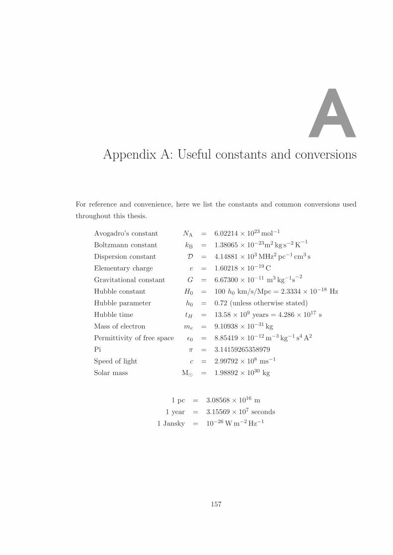
AAppendix A: Useful constants and conversions
For reference and convenience, here we list the constants and common conversions used
throughout this thesis.
Avogadro’s constant NA = 6.02214 × 10²³ mol−1
Boltzmann constant kB = 1.38065 × 10⁻²³m2 kg s−2 K−1
Dispersion constant D = 4.14881 × 10³ MHz2 pc−1 cm3 s
Elementary charge e = 1.60218 × 10⁻¹⁹ C
Gravitational constant G = 6.67300 × 10⁻¹¹ m3 kg−1s−2
Hubble constant H0 = 100 h0 km/s/Mpc = 2.3334 × 10⁻¹⁸ Hz
Hubble parameter h0 = 0.72 (unless otherwise stated)
Hubble time tH = 13.58 × 10⁹ years = 4.286 × 10¹⁷ s
Mass of electron me = 9.10938 × 10⁻³¹ kg
Permittivity of free space ǫ0 = 8.85419 × 10⁻¹² m−3 kg−1 s4A2
Pi π = 3.14159265358979
Speed of light c = 2.99792 × 10⁸ ms−1
Solar mass M⊙ = 1.98892 × 1030 kg
1 pc = 3.08568 × 10¹⁶ m
1 year = 3.15569 × 10⁷ seconds
1 Jansky = 10−26 Wm−2Hz−1
157