supervised descriptive rule discovery: a unifying survey of

Journal of Machine Learning Research 10 (2009) 377-403 Submitted 1/08; Revised 8/08; Published 2/09

Supervised Descriptive Rule Discovery: A Unifying Survey ofContrast Set, Emerging Pattern and Subgroup Mining

Petra Kralj Novak PETRA.KRALJ.NOVAK @IJS.SI

Nada Lavrac∗ NADA .LAVRAC @IJS.SI

Department of Knowledge TechnologiesJozef Stefan InstituteJamova 39, 1000 Ljubljana, Slovenia

Geoffrey I. Webb [email protected]

Faculty of Information TechnologyMonash UniversityBuilding 63, Clayton Campus, Wellington Road, ClaytonVIC 3800, Australia

Editor: Stefan Wrobel

AbstractThis paper gives a survey of contrast set mining (CSM), emerging pattern mining (EPM), and sub-group discovery (SD) in a unifying framework namedsupervised descriptive rule discovery. Whileall these research areas aim at discovering patterns in the form of rules induced from labeled data,they use different terminology and task definitions, claim to have different goals, claim to use dif-ferent rule learning heuristics, and use different means for selecting subsets of induced patterns.This paper contributes a novel understanding of these subareas of data mining by presenting a uni-fied terminology, by explaining the apparent differences between the learning tasks as variants ofa unique supervised descriptive rule discovery task and by exploring the apparent differences be-tween the approaches. It also shows that various rule learning heuristics used in CSM, EPM and SDalgorithms all aim at optimizing a trade off between rule coverage and precision. The commonali-ties (and differences) between the approaches are showcased on a selection of best known variantsof CSM, EPM and SD algorithms. The paper also provides a critical survey of existing superviseddescriptive rule discovery visualization methods.Keywords: descriptive rules, rule learning, contrast set mining, emerging patterns, subgroupdiscovery

1. Introduction

Symbolic data analysis techniques aim at discovering comprehensible patterns or models in data.They can be divided into techniques forpredictive induction, where models, typically induced fromclass labeled data, are used to predict the class value of previously unseen examples, anddescriptiveinduction, where the aim is to find comprehensible patterns, typically induced from unlabeled data.Until recently, these techniques have been investigated by two different research communities: pre-dictive induction mainly by the machine learning community, and descriptive induction mainly bythe data mining community.

∗. Also at University of Nova Gorica, Vipavska 13, 5000 Nova Gorica, Slovenia.

c©2009 Petra Kralj Novak, Nada Lavrac and Geoffrey I. Webb.

KRALJ NOVAK , LAVRA C AND WEBB

Data mining tasks where the goal is to find humanly interpretable differences between groupshave been addressed by both communities independently. The groups canbe interpreted as classlabels, so the data mining community, using the association rule learning perspective, adapted as-sociation rule learners like Apriori by Agrawal et al. (1996) to performa task namedcontrast setmining (Bay and Pazzani, 2001) andemerging pattern mining(Dong and Li, 1999). On the otherhand, the machine learning community, which usually deals with class labeled data, was challengedby, instead of building sets of classification/prediction rules (e.g., Clark andNiblett, 1989; Cohen,1995), to build individual rules for exploratory data analysis and interpretation, which is the goal ofthe task namedsubgroup discovery(Wrobel, 1997).

This paper gives a survey of contrast set mining (CSM), emerging pattern mining (EPM), andsubgroup discovery (SD) in a unifying framework, namedsupervised descriptive rule discovery.Typical applications of supervised descriptive rule discovery include patient risk group detectionin medicine, bioinformatics applications like finding sets of overexpressed genes for specific treat-ments in microarray data analysis, and identifying distinguishing features of different customer seg-ments in customer relationship management. The main aim of these applications is to understandthe underlying phenomena and not to classify new instances. Take another illustrative example,where a manufacturer wants to know in what circumstances his machines may break down; hisintention is not to predict breakdowns, but to understand the factors thatlead to them and how toavoid them.

The main contributions of this paper are as follows. It provides a survey of supervised de-scriptive rule discovery approaches addressed in different communities, and proposes a unifyingsupervised descriptive rule discovery framework, including a critical survey of visualization meth-ods. The paper is organized as follows: Section 2 gives a survey of past research done in the mainsupervised descriptive rule discovery areas: contrast set mining, emerging pattern mining, subgroupdiscovery and other related approaches. Section 3 is dedicated to unifyingthe terminology, defini-tions and the heuristics. Section 4 addresses visualization as an important open issue in superviseddescriptive rule discovery. Section 5 provides a short summary.

2. A Survey of Supervised Descriptive Rule Discovery Approaches

Research on finding interesting rules from class labeled data evolved independently in three distinctareas—contrast set mining, mining of emerging patterns and subgroup discovery—each area usingdifferent frameworks and terminology. In this section, we provide a survey of these three researchareas. We also discuss other related approaches.

2.1 An Illustrative Example

Let us illustrate contrast set mining, emerging pattern mining and subgroup discovery using datafrom Table 1, a very small, artificial sample data set,1 adapted from Quinlan (1986). The data setcontains the results of a survey on 14 individuals, concerning the approval or disapproval of anissue analyzed in the survey. Each individual is characterized by fourattributes—Education (withvaluesprimary school,secondary school, oruniversity), MaritalStatus (single, married,or divorced), Sex (male or female), andHasChildren (yes or no)—that encode rudimentaryinformation about the sociodemographic background. The last columnApproved is the designated

1. Thanks to Johannes Furnkranz for providing this data set.

378

SUPERVISEDDESCRIPTIVERULE DISCOVERY

Education Marital Status Sex Has ChildrenApproved

primary single male no noprimary single male yes noprimary married male no yes

university divorced female no yesuniversity married female yes yessecondary single male no nouniversity single female no yessecondary divorced female no yessecondary single female yes yessecondary married male yes yesprimary married female no yes

secondary divorced male yes nouniversity divorced female yes nosecondary divorced male no yes

Table 1: A sample database.

Marital Stat

0.35714.0

Sex

0.6005.0

single

no

1.0003.0

male

yes

0.0002.0

female

yes

0.0004.0

married

Has Childre

0.4005.0

divorced

yes

0.0003.0

no

no

1.0002.0

yes

Figure 1: A decision tree, modeling the data set shown in Table 1.

classattribute, encoding whether the individual approved or disapproved theissue. Since there isno need for expert knowledge to interpret the results, this data set is appropriate for illustratingthe results of supervised descriptive rule discovery algorithms, whose task is to find interestingpatterns describing individuals that are likely to approve or disapprove the issue, based on the fourdemographic characteristics.

The task ofpredictive inductionis to induce, from a given set oftraining examples, a domainmodel aimed at predictive or classification purposes, such as thedecision treeshown in Figure 1, ora rule setshown in Figure 2, as learned by C4.5 and C4.5rules (Quinlan, 1993), respectively, fromthe sample data in Table 1.

Sex = female → Approved = yesMaritalStatus = single AND Sex = male → Approved = noMaritalStatus = married → Approved = yesMaritalStatus = divorced AND HasChildren = yes → Approved = noMaritalStatus = divorced AND HasChildren = no → Approved = yes

Figure 2: A set of predictive rules, modeling the data set shown in Table 1.

379


MaritalStatus = single AND Sex = male → Approved = noSex = male → Approved = noSex = female → Approved = yesMaritalStatus = married → Approved = yesMaritalStatus = divorced AND HasChildren = yes → Approved = noMaritalStatus = single → Approved = no

Figure 3: Selected descriptive rules, describing individual patterns in the data of Table 1.

In contrast to predictive induction algorithms,descriptive inductionalgorithms typically resultin rules induced from unlabeled examples. E.g., given the examples listed in Table 1, these al-gorithms would typically treat the classApproved no differently from any other attribute. Note,however, that in the learning framework discussed in this paper, that is, inthe framework ofsu-pervised descriptive rule discovery, the discovered rules of the formX →Y are induced from classlabeled data: the class labels are taken into account in learning of patterns of interest, constrainingY at the right hand side of the rule to assign a value to the class attribute.

Figure 3 shows six descriptive rules, found for the sample data using the Magnum Opus (Webb,1995) software. Note that these rules were found using the default settings except that the criticalvalue for the statistical test was relaxed to 0.25. These descriptive rules differ from the predictiverules in several ways. The first rule is redundant with respect to the second. The first is included asa strong pattern (all 3 single males do not approve) whereas the second is weaker but more general(4 out of 7 males do not approve, which is not highly predictive, but accounts for 4 out of all 5respondents who do not approve). Most predictive systems will includeonly one of these rules,but either may be of interest to someone trying to understand the data, depending upon the specificapplication. This particular approach to descriptive pattern discovery does not attempt to secondguess which of the more specific or more general patterns will be the more useful.

Another difference between the predictive and the descriptive rule setsis that the descriptive ruleset does not include the pattern that divorcees without children approve. This is because, while thepattern is highly predictive in the sample data, there are insufficient examplesto pass the statisticaltest which assesses the probability that, given the frequency of respondents approving, the apparentcorrelation occurs by chance. The predictive approach often includes such rules for the sake ofcompleteness, while some descriptive approaches make no attempt at such completeness, assessingeach pattern on its individual merits.

Exactly which rules will be induced by a supervised descriptive rule discovery algorithm de-pends on the task definition, the selected algorithm, as well as the user-defined constraints concern-ing minimal rule support, precision, etc. In the following section, the example set of Table 1 is usedto illustrate the outputs of emerging pattern and subgroup discovery algorithms(see Figures 4 and 5,respectively), while a sample output for contrast set mining is shown in Figure 3 above.

2.2 Contrast Set Mining

The problem of mining contrast sets was first defined by Bay and Pazzani (2001) as finding con-trast sets as “conjunctions of attributes and values that differ meaningfullyin their distributionsacross groups.” The example rules in Figure 3 illustrate this approach, including all conjunctionsof attributes and values that pass a statistical test for productivity (explained below) with respect toattributeApproved that defines the ‘groups.’

380


2.2.1 CONTRAST SET M INING ALGORITHMS

The STUCCO algorithm (Search and Testing for Understandable Consistent Contrasts) by Bay andPazzani (2001) is based on the Max-Miner rule discovery algorithm (Bayardo, 1998). STUCCOdiscovers a set of contrast sets along with their supports2 on groups. STUCCO employs a numberof pruning mechanisms. A potential contrast setX is discarded if it fails a statistical test for inde-pendence with respect to the group variableY. It is also subjected to what Webb (2007) calls a testfor productivity. RuleX →Y is productive iff

∀Z ⊂ X : confidence(Z →Y) < confidence(X →Y)

whereconfidence(X →Y) is a maximum likelihood estimate of conditional probabilityP(Y|X), es-timated by the ratiocount(X,Y)

count(X) , wherecount(X,Y) represents the number of examples for which bothX andY are true, andcount(X) represents the number of examples for whichX is true. Therefore amore specific contrast set must have higher confidence than any of its generalizations. Further testsfor minimum counts and effect sizes may also be imposed.

STUCCO introduced a novel variant of the Bonferroni correction formultiple tests which ap-plies ever more stringent critical values to the statistical tests employed as the number of conditionsin a contrast set is increased. In comparison, the other techniques discussed below do not, by de-fault, employ any form of correction for multiple comparisons, as result of which they have highrisk of makingfalse discoveries(Webb, 2007).

It was shown by Webb et al. (2003) that contrast set mining is a special case of the more generalrule learning task. A contrast set can be interpreted as the antecedent of rule X →Y, and groupGi

for which it is characteristic—in contrast with groupG j—as the rule consequent, leading to rules ofthe formContrastSet→Gi . A standard descriptive rule discovery algorithm, such as an association-rule discovery system (Agrawal et al., 1996), can be used for the taskif the consequent is restrictedto a variable whose values denote group membership.

In particular, Webb et al. (2003) showed that when STUCCO and the general-purpose descrip-tive rule learning system Magnum Opus were each run with their default settings, but the consequentrestricted to the contrast variable in the case of Magnum Opus, the contrasts found differed mainlyas a consequence only of differences in the statistical tests employed to screen the rules.

Hilderman and Peckham (2005) proposed a different approach to contrast set mining calledCIGAR (ContrastIng Grouped Association Rules). CIGAR uses different statistical tests to STUCCOor Magnum Opus for both independence and productivity and introduces a test forminimum sup-port.

Wong and Tseng (2005) have developed techniques for discovering contrasts that can includenegations of terms in the contrast set.

In general, contrast set mining approaches require discrete data, which is in real world appli-cations frequently not the case. A data discretization method developed specifically for set miningpurposes is described by Bay (2000). This approach does not appear to have been further used bythe contrast set mining community, except for Lin and Keogh (2006), who extended contrast setmining to time series and multimedia data analysis. They introduced a formal notion ofa timeseries contrast set along with a fast algorithm to find time series contrast sets. An approach to quan-titative contrast set mining without discretization in the preprocessing phaseis proposed by Simeon

2. The support of a contrast setContrastSetwith respect to a groupGi , support(ContrastSet,Gi), is the percentage ofexamples inGi for which the contrast set is true.

381


and Hilderman (2007) with the algorithm GenQCSets. In this approach, a slightly modified equalwidth binning interval method is used.

Common to most contrast set mining approaches is that they generate all candidate contrast setsfrom discrete (or discretized) data and later use statistical tests to identify theinteresting ones. Openquestions identified by Webb et al. (2003) are yet unsolved: selection ofappropriate heuristics foridentifying interesting contrast sets, appropriate measures of quality for sets of contrast sets, andappropriate methods for presenting contrast sets to the end users.

2.2.2 SELECTED APPLICATIONS OFCONTRAST SET M INING

The contrast mining paradigm does not appear to have been pursued in many published applications.Webb et al. (2003) investigated its use with retail sales data. Wong and Tseng (2005) applied contrastset mining for designing customized insurance programs. Siu et al. (2005)have used contrast setmining to identify patterns in synchrotron x-ray data that distinguish tissue samples of differentforms of cancerous tumor. Kralj et al. (2007b) have addressed a contrast set mining problem ofdistinguishing between two groups of brain ischaemia patients by transformingthe contrast setmining task to a subgroup discovery task.

2.3 Emerging Pattern Mining

Emerging patterns were defined by Dong and Li (1999) as itemsets whose support increases sig-nificantly from one data set to another. Emerging patterns are said to capture emerging trends intime-stamped databases, or to capture differentiating characteristics between classes of data.

2.3.1 EMERGING PATTERN M INING ALGORITHMS

Efficient algorithms for mining emerging patterns were proposed by Dong and Li (1999) and Fanand Ramamohanarao (2003). When first defined by Dong and Li (1999), the purpose of emergingpatterns was “to capture emerging trends in time-stamped data, or useful contrasts between dataclasses”. Subsequent emerging pattern research has largely focused on the use of the discoveredpatterns for classification purposes, for example, classification by emerging patterns (Dong et al.,1999; Li et al., 2000) and classification by jumping emerging patterns3 (Li et al., 2001). An ad-vanced Bayesian approach (Fan and Ramamohanara, 2003) and bagging (Fan et al., 2006) werealso proposed.

From a semantic point of view, emerging patterns are association rules with anitemset in ruleantecedent, and a fixed consequent:ItemSet→ D1, for given data setD1 being compared to anotherdata setD2.

The measure of quality of emerging patterns is thegrowth rate(the ratio of the two supports).It determines, for example, that a pattern with a 10% support in one data setand 1% in the otheris better than a pattern with support 70% in one data set and 10% in the other (as 10

1 >7010). From

the association rule perspective,GrowthRate(ItemSet,D1,D2) = confidence(ItemSet→D1)1−confidence(ItemSet→D1)

. Thus it canbe seen that growth rate provides an identical ordering to confidence, except that growth rate isundefined when confidence = 1.0.

3. Jumping emerging patterns are emerging patterns with support zero inone data set and greater then zero in the otherdata set.

382


MaritalStatus = single AND Sex = male → Approved = noMaritalStatus = married → Approved = yesMaritalStatus = divorced AND HasChildren = yes → Approved = no

Figure 4: Jumping emerging patterns in the data of Table 1.

Some researchers have argued that finding all the emerging patterns above a minimum growthrate constraint generates too many patterns to be analyzed by a domain expert. Fan and Ramamoha-narao (2003) have worked on selecting the interesting emerging patterns,while Soulet et al. (2004)have proposed condensed representations of emerging patterns.

Boulesteix et al. (2003) introduced a CART-based approach to discover emerging patterns inmicroarray data. The method is based on growing decision trees from whichthe emerging patternsare extracted. It combines pattern search with a statistical procedure based on Fisher’s exact test toassess the significance of each emerging pattern. Subsequently, sample classification based on theinferred emerging patterns is performed using maximum-likelihood linear discriminant analysis.

Figure 4 shows all jumping emerging patterns found for the data in Table 1 when using a min-imum support of 15%. These were discovered using the Magnum Opus software, limiting the con-sequent to the variableapproved, setting minimum confidence to 1.0 and setting minimum supportto 2.

2.3.2 SELECTED APPLICATIONS OFEMERGING PATTERNS

Emerging patterns have been mainly applied to the field of bioinformatics, more specifically tomicroarray data analysis. Li et al. (2003) present an interpretable classifier based on simple rules thatis competitive to the state of the art black-box classifiers on the acute lymphoblastic leukemia (ALL)microarray data set. Li and Wong (2002) have focused on finding groups of genes by emergingpatterns and applied it to the ALL/AML data set and the colon tumor data set. Song et al. (2001) usedemerging patterns together with unexpected change and the added/perished rule to mine customerbehavior.

2.4 Subgroup Discovery

The task of subgroup discovery was defined by Klosgen (1996) and Wrobel (1997) as follows:“Given a population of individuals and a property of those individuals that we are interested in, findpopulation subgroups that are statistically ‘most interesting’, for example, are as large as possibleand have the most unusual statistical (distributional) characteristics with respect to the property ofinterest”.

2.4.1 SUBGROUPDISCOVERY ALGORITHMS

Subgroup descriptions are conjunctions of features that are characteristic for a selected class ofindividuals (property of interest). A subgroup description can be seenas the condition part of a ruleSubgroupDescription→Class. Therefore, subgroup discovery can be seen as a special case ofamore general rule learning task.

Subgroup discovery research has evolved in several directions. Onthe one hand, exhaustiveapproaches guarantee the optimal solution given the optimization criterion. One system that canuse both exhaustive and heuristic discovery algorithms is Explora by Klosgen (1996). Other algo-

383


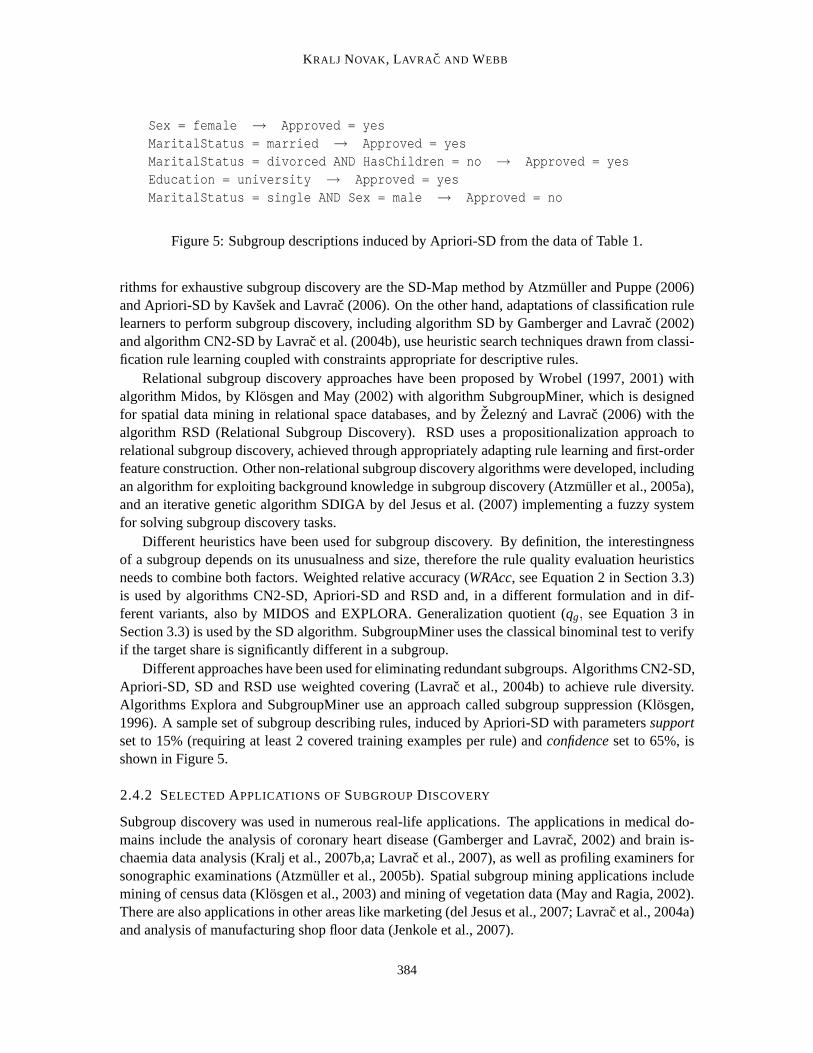
Sex = female → Approved = yesMaritalStatus = married → Approved = yesMaritalStatus = divorced AND HasChildren = no → Approved = yesEducation = university → Approved = yesMaritalStatus = single AND Sex = male → Approved = no

Figure 5: Subgroup descriptions induced by Apriori-SD from the data ofTable 1.

rithms for exhaustive subgroup discovery are the SD-Map method by Atzmuller and Puppe (2006)and Apriori-SD by Kavsek and Lavrac (2006). On the other hand, adaptations of classification rulelearners to perform subgroup discovery, including algorithm SD by Gamberger and Lavrac (2002)and algorithm CN2-SD by Lavrac et al. (2004b), use heuristic search techniques drawn from classi-fication rule learning coupled with constraints appropriate for descriptiverules.

Relational subgroup discovery approaches have been proposed byWrobel (1997, 2001) withalgorithm Midos, by Klosgen and May (2002) with algorithm SubgroupMiner, which is designedfor spatial data mining in relational space databases, and byZelezny and Lavrac (2006) with thealgorithm RSD (Relational Subgroup Discovery). RSD uses a propositionalization approach torelational subgroup discovery, achieved through appropriately adapting rule learning and first-orderfeature construction. Other non-relational subgroup discovery algorithms were developed, includingan algorithm for exploiting background knowledge in subgroup discovery (Atzmuller et al., 2005a),and an iterative genetic algorithm SDIGA by del Jesus et al. (2007) implementing a fuzzy systemfor solving subgroup discovery tasks.

Different heuristics have been used for subgroup discovery. By definition, the interestingnessof a subgroup depends on its unusualness and size, therefore the rulequality evaluation heuristicsneeds to combine both factors. Weighted relative accuracy (WRAcc, see Equation 2 in Section 3.3)is used by algorithms CN2-SD, Apriori-SD and RSD and, in a different formulation and in dif-ferent variants, also by MIDOS and EXPLORA. Generalization quotient (qg, see Equation 3 inSection 3.3) is used by the SD algorithm. SubgroupMiner uses the classical binominal test to verifyif the target share is significantly different in a subgroup.

Different approaches have been used for eliminating redundant subgroups. Algorithms CN2-SD,Apriori-SD, SD and RSD use weighted covering (Lavrac et al., 2004b) to achieve rule diversity.Algorithms Explora and SubgroupMiner use an approach called subgroup suppression (Klosgen,1996). A sample set of subgroup describing rules, induced by Apriori-SD with parameterssupportset to 15% (requiring at least 2 covered training examples per rule) andconfidenceset to 65%, isshown in Figure 5.

2.4.2 SELECTED APPLICATIONS OFSUBGROUPDISCOVERY

Subgroup discovery was used in numerous real-life applications. The applications in medical do-mains include the analysis of coronary heart disease (Gamberger and Lavrac, 2002) and brain is-chaemia data analysis (Kralj et al., 2007b,a; Lavrac et al., 2007), as well as profiling examiners forsonographic examinations (Atzmuller et al., 2005b). Spatial subgroup mining applications includemining of census data (Klosgen et al., 2003) and mining of vegetation data (May and Ragia, 2002).There are also applications in other areas like marketing (del Jesus et al., 2007; Lavrac et al., 2004a)and analysis of manufacturing shop floor data (Jenkole et al., 2007).

384


2.5 Related Approaches

Research in some closely related areas of rule learning, performed independently from the abovedescribed approaches, is outlined below.

2.5.1 CHANGE M INING

The paper by Liu et al. (2001) onfundamental rule changesproposes a technique to identify theset of fundamental changes in two given data sets collected from two time periods. The proposedapproach first generates rules and in the second phase it identifies changes (rules) that can not beexplained by the presence of other changes (rules). This is achieved by applying statisticalχ2 testfor homogeneity of support and confidence. This differs from contrast set discovery through itsconsideration of rules for each group, rather than itemsets. A change in the frequency of just oneitemset between groups may affect many association rules, potentially all rules that have the itemsetas either an antecedent or consequent.

Liu et al. (2000) and Wang et al. (2003) present techniques that identify differences in thedecision trees and classification rules, respectively, found on two different data sets.

2.5.2 MINING CLOSED SETS FROMLABELED DATA

Closed sets have been proven successful in the context of compacted data representation for asso-ciation rule learning. However, their use is mainly descriptive, dealing only with unlabeled data. Itwas recently shown that when considering labeled data, closed sets can be adapted for classificationand discrimination purposes by conveniently contrasting covering properties on positive and nega-tive examples (Garriga et al., 2006). The approach was successfully applied in potato microarraydata analysis to a real-life problem of distinguishing between virus sensitiveand resistant transgenicpotato lines (Kralj et al., 2006).

2.5.3 EXCEPTION RULE M INING

Exception rule mining considers a problem of finding a set of rule pairs, each of which consistsof an exception rule (which describes a regularity for fewer objects) associated with a strong rule(description of a regularity for numerous objects with few counterexamples). An example of sucha rule pair is “using a seat belt is safe” (strong rule) and “using a seat belt is risky for a child”(exception rule). While the goal of exception rule mining is also to find descriptive rules fromlabeled data, in contrast with other rule discovery approaches described in this paper, the goal ofexception rule mining is to find “weak” rules—surprising rules that are an exception to the generalbelief of background knowledge.

Suzuki (2006) and Daly and Taniar (2005), summarizing the research inexception rule mining,reveal that the key concerns addressed by this body of research include interestingness measures,reliability evaluation, practical application, parameter reduction and knowledge representation, aswell as providing fast algorithms for solving the problem.

2.5.4 IMPACT RULES, BUMP HUNTING, QUANTITATIVE ASSOCIATIONRULES

Supervised descriptive rule discovery seeks to discover sets of conditions that are related to devia-tions in the class distribution, where the class is a qualitative variable. A relatedbody of researchseeks to discover sets of conditions that are related to deviations in a targetquantitative variable.

385


Contrast Set Mining Emerging Pattern Mining Subgroup Discovery Rule Learning

contrast set itemset subgroup description rule conditiongroupsG1, . . .Gn data setsD1 andD2 class/propertyC class/conceptCi

attribute-value pair item logical (binary) feature conditionexamples in groups transactions in data sets examples of examples of

G1, . . .Gn D1 andD2 C andC C1 . . .Cn

examples for which transactions containing subgroup of instancescovered examplesthe contrast set is true the itemset

support of contrast set onGi support of EP in data setD1 true positive rate true positive ratesupport of contrast set onG j support of EP in data setD2 false positive rate false positive rate

Table 2: Table of synonyms from different communities, showing the compatibility of terms.

Such techniques include Bump Hunting (Friedman and Fisher, 1999), Quantitative AssociationRules (Aumann and Lindell, 1999) and Impact Rules (Webb, 2001).

3. A Unifying Framework for Supervised Descriptive Rule Induction

This section presents a unifying framework for contrast set mining, emerging pattern mining andsubgroup discovery, as the main representatives of supervised descriptive rule discovery approaches.This is achieved by unifying the terminology, the task definitions and the rule learning heuristics.

3.1 Unifying the Terminology

Contrast set mining (CSM), emerging pattern mining (EPM) and subgroup discovery (SD) weredeveloped in different communities, each developing their own terminology that needs to be clar-ified before proceeding. Below we show that terms used in different communities are compatible,according to the following definition of compatibility.

Definition 1: Compatibility of terms. Terms used in different communities are compatible if theycan be translated into equivalent logical expressions and if they bare the same meaning, that is, ifterms from one community can replace terms used in another community.

Lemma 1: Terms used in CSM, EPM and SD are compatible.Proof The compatibility of terms is proven through a term dictionary, whose aim is to translate allthe terms used in CSM, EPM and SD into the terms used in the rule learning community.The termdictionary is proposed in Table 2. More specifically, this table provides a dictionary of equivalentterms from contrast set mining, emerging pattern mining and subgroup discovery, in a unifying ter-minology of classification rule learning, and in particular of concept learning (considering classCi

as the concept to be learned from the positive examples of this concept, and the negative examplesformed of examples of all other classes).

3.2 Unifying the Task Definitions

Having established a unifying view on the terminology, the next step is to provide a unifying viewon the different task definitions.

386


CSM A contrast set mining task is defined as follows (Bay and Pazzani, 2001). Let A1, A2, . . . ,Ak be a set ofk variables called attributes. EachAi can take values from the set{vi1, vi2, . . . ,vim}. Given a set of user defined groupsG1, G2, . . . , Gn of data instances, a contrast set isa conjunction of attribute-value pairs, defining a pattern that best discriminates the instancesof different user-defined groups. A special case of contrast setmining considers only twocontrasting groups (G1 andG2). In such cases, we wish to find characteristics of one groupdiscriminating it from the other and vice versa.

EPM An emerging patterns mining task is defined as follows (Dong and Li, 1999). Let I = {i1, i2,. . . , iN} be a set of items (note that an item is equivalent to a binary feature in SD, andanindividual attribute-value pair in CSM). A transaction is a subsetT of I . A datasetis a setD of transactions. A subsetX of I is called anitemset. TransactionT contains an itemsetX in a data setD, if X ⊆ T. For two data setsD1 andD2, emerging pattern mining aims atdiscovering itemsets whose support increases significantly from one dataset to another.

SD In subgroup discovery, subgroups are described as conjunctions of features, where featuresare of the formAi = vi j for nominal attributes, andAi > valueor Ai ≤ valuefor continuousattributes. Given the property of interestC, and the population of examples ofC andC, thesubgroup discovery task aims at finding population subgroups that are as large as possible andhave the most unusual statistical (distributional) characteristics with respect to the propertyof interestC (Wrobel, 1997).

The definitions of contrast set mining, emerging pattern mining and subgroupdiscovery appeardifferent: contrast set mining searches for discriminating characteristicsof groups called contrastsets, emerging pattern mining aims at discovering itemsets whose support increases significantlyfrom one data set to another, while subgroup discovery searches forsubgroup descriptions. By us-ing the dictionary from Table 2 we can see that the goals of these three mining tasks are very similar,it is primarily the terminology that differs.

Definition 2: Compatibility of task definitions. Definitions of different learning tasks are compat-ible if one learning task can be translated into another learning task without substantially changingthe learning goal.

Lemma 2: Definitions of CSM, EPM and SD tasks are compatible.

Proof To show the compatibility of task definitions, we propose a unifying table (Table3) of taskdefinitions, allowing us to see that emerging pattern mining taskEPM(D1,D2) is equivalent toCSM(Gi ,G j). It is also easy to show that a two-group contrast set mining taskCSM(Gi ,G j) can bedirectly translated into the following two subgroup discovery tasks:SD(Gi) for C = Gi andC = G j ,andSD(G j) for C = G j andC = Gi .

387



Given Given Given Givenexamples inG1 vs. G j transactions inD1 andD2 in examplesC examples inCi

from G1, . . .Gi from D1 andD2 from C andC from C1 . . .Cn

Find Find Find FindContrastSetik → Gi ItemSet1k → D1 SubgrDescrk →C {RuleCondik →Ci}ContrastSetj l → G j ItemSet2l → D2

Table 3: Table of task definitions from different communities, showing the compatibility of taskdefinitions in terms of output rules.

Having proved that the subgroup discovery task is compatible with a two-group contrast setmining task, it is by induction compatible with a general contrast set mining task, as shown below.

CSM(G1, . . .Gn)for i=2 to ndo

for j=1, j, i to n-1doSD(C = Gi vs. C = G j)

Note that in Table 3 of task definitions column ‘Rule Learning’ again corresponds to a conceptlearning task instead of the general classification rule learning task. In theconcept learning setting,which is better suited for the comparisons with supervised descriptive rule discovery approaches,a distinguished classCi is learned from examples of this class, and examples of all other classesC1, . . . , Ci−1, Ci+1, CN are merged to form the set of examples of classCi . In this case, inducedrule set{RuleCondik → Ci} consists only of rules for distinguished classCi . On the other hand,in a general classification rule learning setting, from examples ofN different classes a set of ruleswould be learned{. . . , RuleCondik →Ci , RuleCondik+1 →Ci , . . . ,RuleCondj l →Cj , . . . ,Default},consisting of sets of rules of the formRuleCondik →Ci for each individual classCi , supplementedby the default rule.

While the primary tasks are very closely related, each of the three communities has concen-trated on different sets of issues around this task. The contrast set discovery community has paidgreatest attention to the statistical issues of multiple comparisons that, if not addressed, can result inhigh risks of false discoveries. The emerging patterns community has investigated how superviseddescriptive rules can be used for classification. The contrast set andemerging pattern communi-ties have primarily addressed only categorical data whereas the subgroup discovery community hasalso considered numeric and relational data. The subgroup discovery community has also exploredtechniques for discovering small numbers of supervised descriptive rules with high coverage of thedata.

3.3 Unifying the Rule Learning Heuristics

The aim of this section is to provide a unifying view on rule learning heuristics used in differentcommunities. To this end, we first investigate the rule quality measures.

Most rule quality measures are derived by analyzing the covering properties of the rule and theclass in the rule consequent considered as positive. This relationship can be depicted by a confusion

388


predictedactual # of positives # of negatives

# of positives p = |TP(X,Y)| p = |FN(X,Y)| P# of negatives n = |FP(X,Y)| n = |TN(X,Y)| N

p+n p+n P+N

Table 4: Confusion matrix:TP(X,Y) stands for true positives,FP(X,Y) for false positives,FN(X,Y) for false negatives andTN(X,Y) for true negatives, as predicted by ruleX →Y.

matrix (Table 4, see, e.g., Kohavi and Provost, 1998), which considersthat ruleR = X → Y isrepresented as(X,Y), and definesp as the number of true positives (positive examples correctlyclassified as positive by rule(X,Y)), n as the number of false positives, etc., from which othercovering characteristics of a rule can be derived: true positive rateTPr(X,Y) = p

P and false positiverateFPr(X,Y) = n

N .

CSM Contrast set mining aims at discovering contrast sets that best discriminate the instancesof different user-defined groups. The support of contrast setX with respect to groupGi ,support(X,Gi), is the percentage of examples inGi for which the contrast set is true. Notethatsupport of a contrast set with respect to group Gis the same astrue positive ratein theclassification rule and subgroup discovery terminology, that is,support(X,Gi) = count(X,Gi)

|Gi |=

TPr(X,Gi). A derived goal of contrast set mining, proposed by Bay and Pazzani (2001), is tofind contrast sets whose support differs meaningfully across groups, for δ being a user-definedparameter.

SuppDiff(X,Gi ,G j) = |support(X,Gi)−support(X,G j)| ≥ δ.

EPM Emerging pattern mining aims at discovering itemsets whose support increasessignificantlyfrom one data set to another Dong and Li (1999), wheresupportof itemsetX in data setDis computed assupport(X,D) = count(X,D)

|D| , for count(X,D) being the number of transactionsin D containingX. Suppose we are given an ordered pair of data setsD1 and D2. TheGrowthRateof an itemsetX from D1 to D2, denoted asGrowthRate(X,D1,D2), is defined asfollows:

GrowthRate(X,D1,D2) =support(X,D1)

support(X,D2). (1)

Definitions of special cases ofGrowthRate(X,D1,D2) are as follows, ifsupport(X,D1) = 0thenGrowthRate(X,D1,D2) = 0, if support(X,D2) = 0 thenGrowthRate(X,D1,D2) = ∞.

SD Subgroup discovery aims at finding population subgroups that are as large as possible and havethe most unusual statistical (distributional) characteristics with respect to theproperty of in-terest (Wrobel, 1997). There were several heuristics developed and used in the subgroupdiscovery community. Since they follow from the task definition, they try to maximizesub-group size and the distribution difference at the same time. Examples of such heuristics aretheweighted relative accuracy(Equation 2, see Lavrac et al., 2004b) and thegeneralization

389



SuppDiff(X,Gi ,G j ) WRAcc(X,C) Piatetski-Shapiro heuristicleverage

GrowthRate(X,D1,D2) qg(X,C) odds ratio forg = 0accuracy/precision, forg = p

Table 5: Table of relationships between the pairs of heuristics, and their equivalents in classificationrule learning.

quotient(Equation 3, see Gamberger and Lavrac, 2002) , forg being a user-defined parameter.

WRAcc(X,C) =p+nP+N

·

(

pp+n

−P

P+N

)

, (2)

qg(X,C) =p

n+g. (3)

Let us now investigate whether the heuristics used in CSM, EPM and SD are compatible, usingthe following definition of compatibility.

Definition 3: Compatibility of heuristics.Heuristic function h1 is compatiblewith h2 if h2 can be derived from h1 and if for any two rules Rand R′, h1(R) > h1(R′) ⇔ h2(R) > h2(R′).

Lemma 3: Definitions of CSM, EPM and SD heuristics are pairwise compatible.Proof The proof of Lemma 3 is established by proving two sub-lemmas, Lemma 3a and Lemma 3b,which prove the compatibility of two pairs of heuristics, whereas the relationships between thesepairs is established through Table 5, and illustrated in Figures 6 and 7.

Lemma 3a: The support difference heuristic used in CSM and the weighted relative accuracyheuristic used in SD are compatible.Proof Note that, as shown below, weighted relative accuracy (Equation 2) can be interpreted interms of probabilities of rule antecedentX and consequentY (classC representing the property ofinterest), and the conditional probability of classY givenX, estimated by relative frequencies.

WRAcc(X,Y) = P(X) · (P(Y|X)−P(Y)).

From this equation we see that, indeed, when optimizing weighted relative accuracy of ruleX →Y,we optimize two contrasting factors: rule coverageP(X) (proportional to the size of the subgroup),and distributional unusualnessP(Y|X)−P(Y) (proportional to the difference of the number of posi-tive examples correctly covered by the rule and the number of positives in the original training set).It is straightforward to show that this measure is equivalent to the Piatetski-Shapiro measure, whichevaluates the conditional (in)dependence of rule consequent and ruleantecedent as follows:

PS(X,Y) = P(X ·Y)−P(X) ·P(Y).

390


Weighted relative accuracy, known from subgroup discovery, and support difference betweengroups, used in contrast set mining, are related as follows:4

WRAcc(X,Y) == P(X) · [P(Y|X)−P(Y)] = P(Y ·X)−P(Y) ·P(X)= P(Y ·X)−P(Y) · [P(Y ·X)+P(Y ·X)]= (1−P(Y)) ·P(Y ·X)−P(Y) ·P(Y ·X)= P(Y) ·P(Y) ·P(X|Y)−P(Y) ·P(Y) ·P(X|Y)= P(Y) ·P(Y) · [P(X|Y)−P(X|Y)]= P(Y) ·P(Y) · [TPr(X,Y)−FPr(X,Y)].

Since the distribution of examples among classes is constant for any data set,the first two factorsP(Y) and P(Y) are constant within a data set. Therefore, when maximizing the weighted relativeaccuracy, one is maximizing the second factorTPr(X,Y)−FPr(X,Y), which actually is supportdifference when we have a two group contrast set mining problem. Consequently, forC = G1, andC = G2 the following holds:

WRAcc(X,C) = WRAcc(X,G1) = P(G1) ·P(G2) · [support(X,G1)−support(X,G2)].

Lemma 3b: The growth rate heuristic used in EPM and the generalization quotient heuristic usedin SD are compatible.Proof Equation 1 can be rewritten as follows:

GrowthRate(X,D1,D2) =support(X,D1)

support(C,D2)=

=count(X,D1)

count(X,D2)·|D2|

|D1|=

pn·NP

.

Since the distribution of examples among classes is constant for any data set,the quotientNP isconstant. Consequently, the growth rate is the generalization quotient withg = 0, multiplied by aconstant. Therefore, the growth rate is compatible with the generalization quotient.

GrowthRate(X,C,C) = q0(X,C) ·NP

.

The lemmas prove that heuristics used in CSM and EPM can be translated into heuristics used inSD and vice versa. In this way, we have shown the compatibility of CSM and SDheuristics, as wellas the compatibility of EPM and SD heuristics. While the lemmas do not prove directcompatibilityof CSM and EPM heuristics, they prove that heuristics used in CSM and EPMcan be translated intotwo heuristics used in SD, both aiming at trading-off between coverage anddistributional difference.

4. Peter A. Flach is acknowledged for having derived these equations.

391


Figure 6: Isometrics forqg. The dotted lines show the isometrics for a selectedg> 0, while the fulllines show the special case wheng = 0, compatible to the EPMgrowth rateheuristic.

Figure 7: Isometrics forWRAcc, compatible to the CSMsupport differenceheuristic.

Table 5 provides also the equivalents of these heuristics in terms of heuristics known fromthe classification rule learning community, details of which are beyond the scope of this paper(an interested reader can find more details on selected heuristics and their ROC representations inFurnkranz and Flach, 2003).

Note that the growth rate heuristic from EPM, as a special case of the generalization quotientheuristic withg= 0, does not consider rule coverage. On the other hand, its compatible counterpart,the generalization quotientqg heuristic used in SD, can be tailored to favor more general rules bysetting theg parameter value, as for a generalg value, theqg heuristic provides a trade-off betweenrule accuracy and coverage. Figure 65 illustrates theqg isometrics, for a generalg value, as well asfor valueg = 0.

Note also that standard rule learners (such as CN2 by Clark and Niblett, 1989) tend to generatevery specific rules, due to using accuracy heuristicAcc(X,Y) = p+n

P+N or its variants: the Laplaceand them-estimate. On the other hand, the CSM support difference heuristic and its SD counterpartWRAccboth optimize a trade-off between rule accuracy and coverage. TheWRAccisometrics areplotted in Figure 7.6

3.4 Comparison of Rule Selection Mechanisms

Having established a unifying view on the terminology, definitions and rule learning heuristics, thelast step is to analyze rule selection mechanisms used by different algorithms.The motivation forrule selection can be either to find only significant rules or to avoid overlapping rules (too manytoo similar rules), or to avoid showing redundant rules to the end users. Note that rule selection isnot always necessary and that depending on the goal, redundant rules can be valuable (e.g., clas-

5. This figure is due to Gamberger and Lavrac (2002).6. This figure is due to Furnkranz and Flach (2003).

392


sification by aggregating emerging patterns by Dong et al., 1999). Two approaches are commonlyused: statistic tests and the (weighted) covering approach. In this section,we compare these twoapproaches.

Webb et al. (2003) show that contrast set mining is a special case of the more general rulediscovery task. However, an experimental comparison of STUCCO, OPUS AR and C4.5 has shownthat standard rule learners return a larger set of rules compared to STUCCO, and that some of themare also not interesting to end users. STUCCO (see Bay and Pazzani 2001 for more details) usesseveral mechanisms for rule pruning. Statistical significance pruning removes contrast sets that,while significant and large, derive these properties only due to being specializations of more generalcontrast sets: any specialization is pruned that has a similar support to its parent or that fails aχ2

test of independence with respect to its parent.In the context of OPUSAR, the emphasis has been on developing statistical tests that are robust

in the context of the large search spaces explored in many rule discoveryapplications Webb (2007).These include tests for independence between the antecedent and consequent, and tests to assesswhether specializations have significantly higher confidence than their generalizations.

In subgroup discovery, theweighted covering approach(Lavrac et al., 2004b) is used with theaim of ensuring the diversity of rules induced in different iterations of thealgorithm. In each iter-ation, after selecting the best rule, the weights of positive examples are decreased according to thenumber of rules covering each positive examplerule count(e); they are set tow(e) = 1

rule count(e) .For selecting the best rule in consequent iterations, the SD algorithm (Gamberger and Lavrac, 2002)uses—instead of the unweightedqg measure (Equation 3)—the weighted variant ofqg defined inEquation 4, while the CN2-SD (Lavrac et al., 2004b) and APRIORI-SD (Kavsek and Lavrac, 2006)algorithms use the weighted relative accuracy (Equation 2) modified with example weights, as de-fined in Equation 5, wherep′ = ∑TP(X,Y) w(e) is the sum of the weights of all covered positiveexamples, andP′ is the sum of the weights of all positive examples.

q′g(X,Y) =p′

n+g, (4)

WRAcc′(X,Y) =p′ +nP′ +N

·

(

p′

p′ +n−

PP+N

)

. (5)

Unlike in the sections on the terminology, task definitions and rule learning heuristics, the com-parison of rule pruning mechanisms described in this section does not result in a unified view;although the goals of rule pruning may be the same, the pruning mechanisms used in differentsubareas of supervised descriptive rule discovery are—as shown above—very different.

4. Visualization

Webb et al. (2003) identify a need to develop appropriate methods for presenting contrast sets toend users, possibly through contrast set visualization. This open issue, concerning the visualizationof contrast sets and emerging patterns, can be resolved by importing some of the solutions proposedin the subgroup discovery community. Several methods for subgroup visualization were developedby Wettschereck (2002), Wrobel (2001), Gamberger et al. (2002),Kralj et al. (2005) and Atzmullerand Puppe (2005). They are here illustrated using the coronary heartdisease data set, originallyanalyzed by Gamberger and Lavrac (2002). The visualizations are evaluated by considering their

393


Figure 8: Subgroup visualization by pie charts.Figure 9: Subgroup visualization by box plots.

intuitiveness, correctness of displayed data, usefulness, ability to display contents besides the nu-merical properties of subgroups, (e.g., plot subgroup probability densities against the values of anattribute), and their extensibility to multi-class problems.

4.1 Visualization by Pie Charts

Slices of pie charts are the most common way of visualizing parts of a whole. They are widely usedand understood. Subgroup visualization by pie chart, proposed by Wettschereck (2002), consistsof a two-level pie for each subgroup. The base pie represents the distribution of individuals interms of the property of interest of the entire example set. The inner pie represents the size and thedistribution of individuals in terms of the property of interest in a specific subgroup. An example offive subgroups (subgroups A1, A2, B1, B2, C1), as well as the basepie “all subjects” are visualizedby pie charts in Figure 8.

The main weakness of this visualization is the misleading representation of the relative sizeof subgroups. The size of a subgroup is represented by the radius ofthe circle. The faultinessarises from the surface of the circle which increases with the square of itsradius. For example, asubgroup that covers 20% of examples is represented by a circle that covers only 4% of the wholesurface, while a subgroup that covers 50% of examples is representedby a circle that covers 25%of the whole surface. In terms of usefulness, this visualization is not veryhandy since—in order tocompare subgroups—one would need to compare sizes of circles, which isdifficult. The comparisonof distributions in subgroups is also not straightforward. This visualizationalso does not show thecontents of subgroups. It would be possible to extend this visualization to multi-class problems.

4.2 Visualization by Box Plots

In subgroup visualization by box plots, introduced by Wrobel (2001), each subgroup is representedby one box plot (all examples are also considered as one subgroup andare displayed in the topbox). Each box shows the entire population; the horizontally stripped areaon the left representsthe positive examples and the white area on the right-hand side of the box represents the negativeexamples. The grey area within each box indicates the respective subgroup. The overlap of the greyarea with the hatched area shows the overlap of the group with the positive examples. Hence, themore to the left the grey area extends the better. The less the grey area extends to the right of thehatched area, the more specific a subgroup is (less overlap with the subjects of the negative class).Finally, the location of the box along the X-axis indicates the relative share ofthe target class withineach subgroup: the more to the right a box is placed, the higher is the shareof the target value withinthis subgroup. The vertical line (in Figure 9 at value 46.6%) indicates the default accuracy, that is,

394


the number of positive examples in the entire population. An example box plot visualization of fivesubgroups is presented in Figure 9.

On the negative side, the intuitiveness of this visualization is relatively poor since an extensiveexplanation is necessary for understanding it. It is also somewhat illogicalsince the boxes that areplaced more to the right and have more grey color on the left-hand side represent the best subgroups.This visualization is not very attractive since most of the image is white; the greyarea (the part ofthe image that really represents the subgroups) is a relatively tiny part of the entire image. On thepositive side, all the visualized data are correct and the visualization is useful since the subgroupsare arranged by their confidence. It is also easier to contrast the sizesof subgroups compared totheir pie chart visualization. However, this visualization does not display thecontents of the data. Itwould also be difficult to extend this visualization to multi-class problems.

4.3 Visualizing Subgroup Distribution w.r.t. a Continuous Attribute

The distribution of examples w.r.t. a continuous attribute, introduced by Gamberger and Lavrac(2002) and Gamberger et al. (2002), was used in the analysis of several medical domains. It isthe only subgroup visualization method that offers an insight of the visualized subgroups. Theapproach assumes the existence of at least one numeric (or ordered discrete) attribute of expert’sinterest for subgroup analysis. The selected attribute is plotted on the X-axis of the diagram. TheY-axis represents the target variable, or more precisely, the number of instances belonging to targetpropertyC (shown on theY+ axis) or not belonging toC (shown on theY− axis) for the values ofthe attribute on the X-axis. It must be noted that both directions of the Y-axis are used to indicatethe number of instances. The entire data set and two subgroups A1 and B2are visualized by theirdistribution over a continuous attribute in Figure 10.

This visualization method is not completely automatic, since the automatic approach does notprovide consistent results. The automatic approach calculates the number of examples for each valueof the attribute on the X-axis by moving a sliding window and counting the number of examples inthat window. The outcome is a smooth line. The difficulty arises when the attributefrom the X-axisappears in the subgroup description. In such a case, a manual correction is needed for this methodto be realistic.

This visualization method is very intuitive since it practically does not need muchexplanation.It is attractive and very useful to the end user since it offers an insightin the contents of displayed

Figure 10: Subgroup visualization w.r.t. a continuous attribute. For clarity ofthe picture, only thepositive (Y+) side of subgroup A1 is depicted.

395


Figure 11: Representation of subgroups inthe ROC space.

all

A2

C1

B1

B2

A1

Figure 12: Subgroup visualization by barcharts.

examples. However, the correctness of displayed data is questionable. It is impossible to generalizethis visualization to multi-class problems.

4.4 Representation in the ROC Space

The ROC (Receiver Operating Characteristics) (Provost and Fawcett,2001) space is a 2-dimensionalspace that shows classifier (rule/rule set) performance in terms of its falsepositive rate (FPr) plottedon the X-axis, and true positive rate (TPr) plotted on the Y-axis. The ROC space is appropriate formeasuring the success of subgroup discovery, since subgroups whose TPr

FPr tradeoffs are close to themain diagonal (line connecting the points (0, 0) and (1, 1) in the ROC space)can be discardedas insignificant (Kavsek and Lavrac, 2006); the reason is that the rules with theTPr

FPr ration on themain diagonal have the same distribution of covered positives and negatives (TPr= FPr) as thedistribution in the entire data set. An example of five subgroups representedin the ROC space isshown in Figure 11.

Even though the ROC space is an appropriate rule visualization, it is usually used just for theevaluation of discovered rules. The ROC convex hull is the line connectingthe potentially optimalsubgroups. The area under the ROC convex hull (AUC, area under curve) is a measure of quality ofthe resulting ruleset.7

This visualization method is not intuitive to the end user, but is absolutely clear toevery machinelearning expert. The displayed data is correct, but there is no content displayed. An advantage of thismethod compared to the other visualization methods is that it allows the comparison of outcomesof different algorithms at the same time. The ROC space is designed for two-class problems and istherefore inappropriate for multi-class problems.

4.5 Bar Charts Visualization

The visualization by bar charts was introduced by Kralj et al. (2005). Inthis visualization, thepurpose of the first line is to visualize the distribution of the entire example set. The area on theright represents the positive examples and the area on the left represents the negative examples of thetarget class. Each following line represents one subgroup. The positive and the negative examplesof each subgroup are drawn below the positive and the negative examples of the entire example set.Subgroups are sorted by the relative share of positive examples (precision).

7. Note that in terms ofTPrFPr ratio optimality, two subgroups (A1 and B2) are suboptimal, lying below the ROC convex

hull.

396


An example of five subgroups visualized by bar charts is shown in Figure 12. It is simple, un-derstandable and shows all the data correctly. This visualization method allows simple comparisonbetween subgroups and is therefore useful. It is relatively straight-forward to understand and can beextended to multi-class problems. It does not display the contents of data, though.

4.6 Summary of Subgroup Visualization Methods

In this section, we (subjectively) compare the five different subgroup visualization methods by con-sidering their intuitiveness, correctness of displayed data, usefulness, ability to ability to displaycontents besides the numerical properties of subgroups, (e.g., plot subgroup probability densitiesagainst the values of an attribute), and their extensibility to multi-class problems.The summary ofthe evaluation is presented in Table 6.

ContinuousPie chart Box plot attribute ROC Bar chart

Intuitiveness + - + +/- +Correctness - + - + +Usefulness - + + + +Contents - - + - -Multi-class + - - - +

Table 6: Our evaluation of subgroup visualization methods.

Two visualizations score best in Table 6 of our evaluation of subgroup visualization methods:the visualization of subgroups w.r.t. a continuous attribute and the bar chartvisualization. Thevisualization of subgroups w.r.t. a continuous attribute is the only visualization that directly showsthe contents of the data; its main shortcomings are the doubtful correctness of the displayed dataand its difficulty to be extended to multi-class problems. It also requires a continuous or ordereddiscrete attribute in the data. The bar chart visualization combines the good properties of the piechart and the box plot visualization. In Table 6, it only fails in displaying the contents of the data.By using the two best visualizations, one gets a very good understanding of the mining results.

To show the applicability of subgroup discovery visualizations for supervised descriptive rulediscovery, the bar visualizations of results of contrast set mining, jumping emerging patterns andsubgroup discovery on the survey data analysis problem of Section 2 are shown in Figures 13, 14and 15, respectively.

Negatives

1.00

0.60

0.80

0.20

0.00

0.40

0.60

1.00

0.00

0.33

0.67

0.44

0.00

0.22

Positives Rule

→Approved=yes

MaritalStatus=single AND Sex=male Approved=no→

Sex=male Approved=no→

Sex=female Approved=yes→

MaritalStatus=married Approved=yes→

MaritalStatus=divorced AND HasChildren=yes Approved=no→

MaritalStatus=single Approved=no→

Figure 13: Bar visualization of contrast sets of Figure 3.

397


Negatives

1.00

0.60

0.00

0.40

1.00

0.00

0.44

0.00

Positives Rule

→Approved=yes

MaritalStatus=single AND Sex=male Approved=no→


MaritalStatus=divorced AND HasChildren=yes Approved=no→

Figure 14: Bar visualization of jumping emerging patterns of Figure 4.

Negatives

1.00

0.00

0.00

0.20

0.20

1.00

0.44

0.33

0.67

0.33

Positives Rule

→Approved=yes


MaritalStatus=divorced AND HasChildren=no Approved=yes→

Sex=female Approved=yes→

Education=university Approved=yes→

Figure 15: Bar visualization of subgroups of Figure 5 of individuals whohave approved the issue.

5. Conclusions

Patterns in the form of rules are intuitive, simple and easy for end users to understand. Therefore, itis not surprising that members of different communities have independently addressed superviseddescriptive rule induction, each of them solving similar problems in similar ways and developingvocabularies according to the conventions of their respective research communities.

This paper sheds a new light on previous work in this area by providing a systematic compari-son of the terminology, definitions, goals, algorithms and heuristics of contrast set mining (CSM),emerging pattern mining (EPM) and subgroup discovery (SD) in a unifying framework called su-pervised descriptive rule discovery. We have also shown that the heuristics used in CSM and EPMcan be translated into two well-known heuristics used in SD, both aiming at trading-off betweencoverage and distributional difference. In addition, the paper presents a critical survey of exist-ing visualization methods, and shows that some methods used in subgroup discovery can be easilyadapted for use in CSM and EPM.

Acknowledgments

The work of Petra Kralj and Nada Lavrac was funded by the project Knowledge Technologies (grantno. P2-0103) funded by the Slovene National Research Agency, andco-funded by the European 6FPproject IQ -Inductive Queries for Mining Patterns and Models(IST-FP6-516169). Geoff Webb’scontribution to this work has been supported by Australian Research Council Grant DP0772238.

References

Rakesh Agrawal, Heikki Mannila, Ramakrishnan Srikant, Hannu Toivonen, and A. Inkeri Verkamo.Fast discovery of association rules.Advances in Knowledge Discovery and Data Mining, pages307–328, 1996.

Martin Atzmuller and Frank Puppe. Semi-automatic visual subgroup mining using VIKAMINE.Journal of Universal Computer Science (JUCS), Special Issue on Visual Data Mining, 11(11):

398


1752–1765, 2005.

Martin Atzmuller and Frank Puppe. SD-Map - a fast algorithm for exhaustive subgroup discov-ery. In Proceedings of the 10th European Conference on Principles and Practice of KnowledgeDiscovery in Databases (PKDD-06), pages 6–17, 2006.

Martin Atzmuller, Frank Puppe, and Hans-Peter Buscher. Exploiting backgroundknowledge forknowledge-intensive subgroup discovery. InProceedings of the 19th International Joint Confer-ence on Artificial Intelligence (IJCAI-05), pages 647–652, 2005a.

Martin Atzmuller, Frank Puppe, and Hans-Peter Buscher. Profiling examiners using intelligentsubgroup mining. InProceedings of the 10th Workshop on Intelligent Data Analysis in Medicineand Pharmacology (IDAMAP-05), pages 46–51, 2005b.

Yonatan Aumann and Yehuda Lindell. A statistical theory for quantitative association rules. InProceedings of the 5th ACM SIGKDD International Conference on Knowledge Discovery andData Mining (KDD-99), pages 261–270, 1999.

Stephen D. Bay. Multivariate discretization of continuous variables for set mining. InProceedingsof the 6th ACM SIGKDD International Conference on Knowledge Discovery and Data Mining(KDD-2000), pages 315–319, 2000.

Stephen D. Bay and Michael J. Pazzani. Detecting group differences:Mining contrast sets.DataMining and Knowledge Discovery, 5(3):213–246, 2001.

Roberto J. Bayardo. Efficiently mining long patterns from databases. InProceedings of the 1998ACM SIGMOD International Conference on Management of Data (SIGMOD-98), pages 85–93,1998.

Anne-Laure Boulesteix, Gerhard Tutz, and Korbinian Strimmer. A CART-based approach to dis-cover emerging patterns in microarray data.Bioinformatics, 19(18):2465–2472, 2003.

Peter Clark and Tim Niblett. The CN2 induction algorithm.Machine Learning, 3(4):261–283,1989.

William W. Cohen. Fast effective rule induction. InProceedings of the 12th International Confer-ence on Machine Learning (ICML-95), pages 115–123, 1995.

Olena Daly and David Taniar. Exception rules in data mining. InEncyclopedia of InformationScience and Technology (II), pages 1144–1148. 2005.

Marıa Jose del Jesus, Pedro Gonzalez, Francisco Herrera, and Mikel Mesonero. Evolutionary fuzzyrule induction process for subgroup discovery: A case study in marketing. IEEE Transactions onFuzzy Systems, 15(4):578–592, 2007.

Guozhu Dong and Jinyan Li. Efficient mining of emerging patterns: Discovering trends and differ-ences. InProceedings of the 5th ACM SIGKDD International Conference on Knowledge Discov-ery and Data Mining (KDD-99), pages 43–52, 1999.

399


Guozhu Dong, Xiuzhen Zhang, Limsoon Wong, and Jinyan Li. CAEP: Classification by aggregatingemerging patterns. InProceedings of the 2nd International Conference on Discovery Science(DS-99), pages 30–42, 1999.

Hongjian Fan and Kotagiri Ramamohanara. A bayesian approach to use emerging patterns forclassification. InProceedings of the 14th Australasian Database Conference (ADC-03), pages39–48, 2003.

Hongjian Fan and Kotagiri Ramamohanarao. Efficiently mining interesting emerging patterns. InProceeding of the 4th International Conference on Web-Age InformationManagement (WAIM-03), pages 189–201, 2003.

Hongjian Fan, Ming Fan, Kotagiri Ramamohanarao, and Mengxu Liu. Further improving emergingpattern based classifiers via bagging. InProceedings of the 10th Pacific-Asia Conference onKnowledge Discovery and Data Mining (PAKDD-06), pages 91–96, 2006.

Jerome H. Friedman and Nicholas I. Fisher. Bump hunting in high-dimensionaldata.Statistics andComputing, 9(2):123–143, 1999.

Johannes Furnkranz and Peter A. Flach. An analysis of rule evaluation metrics. InProceedings ofthe 20th International Conference on Machine Learning (ICML-03), pages 202–209, 2003.

Dragan Gamberger and Nada Lavrac. Expert-guided subgroup discovery: Methodology and appli-cation.Journal of Artificial Intelligence Research, 17:501–527, 2002.

Dragan Gamberger, Nada Lavrac, and Dietrich Wettschereck. Subgroup visualization: A methodand application in population screening. InProceedings of the 7th International Workshop onIntelligent Data Analysis in Medicine and Pharmacology (IDAMAP-02), pages 31–35, 2002.

Gemma C. Garriga, Petra Kralj, and Nada Lavrac. Closed sets for labeled data. InProceedings ofthe 10th European Conference on Principles and Practice of Knowledge Discovery in Databases(PKDD-06), pages 163 – 174, 2006.

Robert J. Hilderman and Terry Peckham. A statistically sound alternative approach to mining con-trast sets. InProceedings of the 4th Australia Data Mining Conference (AusDM-05), pages 157–172, 2005.

Joze Jenkole, Petra Kralj, Nada Lavrac, and Alojzij Sluga. A data mining experiment on manu-facturing shop floor data. InProceedings of the 40th International Seminar on ManufacturingSystems (CIRP-07), 2007. 6 pages.

Branko Kavsek and Nada Lavrac. APRIORI-SD: Adapting association rule learning to subgroupdiscovery.Applied Artificial Intelligence, 20(7):543–583, 2006.

Willi Kl osgen. Explora: A multipattern and multistrategy discovery assistant.Advances in Knowl-edge Discovery and Data Mining, pages 249–271, 1996.

Willi Kl osgen and Michael May. Spatial subgroup mining integrated in an object-relational spatialdatabase. InProceedings of the 6th European Conference on Principles and Practiceof Knowl-edge Discovery in Databases (PKDD-02), pages 275–286, 2002.

400


Willi Kl osgen, Michael May, and Jim Petch. Mining census data for spatial effects on mortality.Intelligent Data Analysis, 7(6):521–540, 2003.

Ron Kohavi and Foster Provost, editors.Editorial for the Special Issue on Applications of MachineLearning and the Knowledge Discovery Process, Glossary of Terms, 1998.

Petra Kralj, Nada Lavrac, and Blaz Zupan. Subgroup visualization. In8th International Multicon-ference Information Society (IS-05), pages 228–231, 2005.

Petra Kralj, Ana Rotter, Natasa Toplak, Kristina Gruden, Nada Lavrac, and Gemma C. Garriga.Application of closed itemset mining for class labeled data in functional genomics. InformaticaMedica Slovenica, (1):40–45, 2006.

Petra Kralj, Nada Lavrac, Dragan Gamberger, and Antonija Krstacic. Contrast set mining for dis-tinguishing between similar diseases. InProceedings of the 11th Conference on Artificial Intelli-gence in Medicine (AIME-07), pages 109–118, 2007a.

Petra Kralj, Nada Lavrac, Dragan Gamberger, and Antonija Krstacic. Contrast set mining throughsubgroup discovery applied to brain ischaemia data. InProceedings of the 11th Pacific-AsiaConference on Advances in Knowledge Discovery and Data Mining : (PAKDD-07), pages 579–586, 2007b.

Nada Lavrac, Bojan Cestnik, Dragan Gamberger, and Peter A. Flach. Decision support throughsubgroup discovery: Three case studies and the lessons learned.Machine Learning Special issueon Data Mining Lessons Learned, 57(1-2):115–143, 2004a.

Nada Lavrac, Branko Kavsek, Peter A. Flach, and Ljupco Todorovski. Subgroup discovery withCN2-SD.Journal of Machine Learning Research, 5:153–188, 2004b.

Nada Lavrac, Petra Kralj, Dragan Gamberger, and Antonija Krstacic. Supporting factors to improvethe explanatory potential of contrast set mining: Analyzing brain ischaemia data. InProceedingsof the 11th Mediterranean Conference on Medical and Biological Engineering and Computing(MEDICON-07), pages 157–161, 2007.

Jinyan Li and Limsoon Wong. Identifying good diagnostic gene groups from gene expressionprofiles using the concept of emerging patterns.Bioinformatics, 18(10):1406–1407, 2002.

Jinyan Li, Guozhu Dong, and Kotagiri Ramamohanarao. Instance-based classification by emerg-ing patterns. InProceedings of the 14th European Conference on Principles and Practice ofKnowledge Discovery in Databases (PKDD-2000), pages 191–200, 2000.

Jinyan Li, Guozhu Dong, and Kotagiri Ramamohanarao. Making use of themost expressive jump-ing emerging patterns for classification.Knowledge and Information Systems, 3(2):1–29, 2001.

Jinyan Li, Huiqing Liu, James R. Downing, Allen Eng-Juh Yeoh, and LimsoonWong. Simple rulesunderlying gene expression profiles of more than six subtypes of acute lymphoblastic leukemia(ALL) patients.Bioinformatics, 19(1):71–78, 2003.

Jessica Lin and Eamonn Keogh. Group SAX: Extending the notion of contrast sets to time series andmultimedia data. InProceedings of the 10th European Conference on Principles and Practice ofKnowledge Discovery in Databases (PKDD-06), pages 284–296, 2006.

401


Bing Liu, Wynne Hsu, Heng-Siew Han, and Yiyuan Xia. Mining changes for real-life applica-tions. InProceedings of the 2nd International Conference on Data Warehousingand KnowledgeDiscovery (DaWaK-2000), pages 337–346, 2000.

Bing Liu, Wynne Hsu, and Yiming Ma. Discovering the set of fundamental rule changes. InProceedings of the 7th ACM SIGKDD International Conference on Knowledge Discovery andData Mining (KDD-01), pages 335–340, 2001.

Michael May and Lemonia Ragia. Spatial subgroup discovery applied to theanalysis of vegetationdata. InProceedings of the 4th International Conference on Practical Aspects of KnowledgeManagement (PAKM-2002), pages 49–61, 2002.

Foster J. Provost and Tom Fawcett. Robust classification for imprecise environments. MachineLearning, 42(3):203–231, 2001.

J. Ross Quinlan. Induction of decision trees.Machine Learning, 1(1):81–106, 1986.

J. Ross Quinlan.C4.5: Programs for Machine Learning. Morgan Kaufmann, 1993.

Mondelle Simeon and Robert J. Hilderman. Exploratory quantitative contrast set mining: A dis-cretization approach. InProceedings of the 19th IEEE International Conference on Tools withArtificial Intelligence - Vol.2 (ICTAI-07), pages 124–131, 2007.

K.K.W. Siu, S.M. Butler, T. Beveridge, J.E. Gillam, C.J. Hall, A.H. Kaye, R.A. Lewis, K. Mannan,G. McLoughlin, S. Pearson, A.R. Round, E. Schultke, G.I. Webb, and S.J. Wilkinson. Identifyingmarkers of pathology in SAXS data of malignant tissues of the brain.Nuclear Instruments andMethods in Physics Research A, 548:140–146, 2005.

Hee S. Song, Jae K. Kimb, and Soung H. Kima. Mining the change of customerbehavior in aninternet shopping mall.Expert Systems with Applications, 21(3):157–168, 2001.

Arnaud Soulet, Bruno Crmilleux, and Franois Rioult. Condensed representation of emerging pat-terns. InProceedings of the 8th Pacific-Asia Conference on Knowledge Discovery and DataMining (PAKDD-04), pages 127–132, 2004.

Einoshin Suzuki. Data mining methods for discovering interesting exceptions from an unsupervisedtable.Journal of Universal Computer Science, 12(6):627–653, 2006.

Ke Wang, Senqiang Zhou, Ada W.-C. Fu, and Jeffrey X. Yu. Mining changes of classificationby correspondence tracing. InProceedings of the 3rd SIAM International Conference on DataMining (SDM-03), pages 95–106, 2003.

Geoffrey I. Webb. OPUS: An efficient admissible algorithm for unordered search. Journal ofArtificial Intelligence Research, 3:431–465, 1995.

Geoffrey I. Webb. Discovering associations with numeric variables. InProceedings of the 7th ACMSIGKDD International Conference on Knowledge Discovery and Data Mining (KDD-01), pages383–388, 2001.

Geoffrey I. Webb. Discovering significant patterns.Machine Learning, 68(1):1–33, 2007.

402


Geoffrey I. Webb, Shane M. Butler, and Douglas Newlands. On detecting differences betweengroups. InProceedings of the 9th ACM SIGKDD International Conference on Knowledge Dis-covery and Data Mining (KDD-03), pages 256–265, 2003.

Dietrich Wettschereck. A KDDSE-independent PMML visualizer. InProceedings of 2nd Workshopon Integration Aspects of Data Mining, Decision Support and Meta-Learning (IDDM-02), pages150–155, 2002.

Tzu-Tsung Wong and Kuo-Lung Tseng. Mining negative contrast setsfrom data with discreteattributes.Expert Systems with Applications, 29(2):401–407, 2005.

Stefan Wrobel. An algorithm for multi-relational discovery of subgroups.In Proceedings of the1st European Conference on Principles of Data Mining and Knowledge Discovery (PKDD-97),pages 78–87, 1997.

Stefan Wrobel. Inductive logic programming for knowledge discovery in databases. In SasoDzeroski and Nada Lavrac, editors,Relational Data Mining, chapter 4, pages 74–101. 2001.

Filip Zelezny and Nada Lavrac. Propositionalization-based relational subgroup discovery withRSD. Machine Learning, 62:33–63, 2006.

403

supervised descriptive rule discovery: a unifying survey of

Documents