supervised evaluation of representations a...
TRANSCRIPT

SUPERVISED EVALUATION OF REPRESENTATIONS
A DISSERTATION
SUBMITTED TO THE DEPARTMENT OF STATISTICS
AND THE COMMITTEE ON GRADUATE STUDIES
OF STANFORD UNIVERSITY
IN PARTIAL FULFILLMENT OF THE REQUIREMENTS
FOR THE DEGREE OF
DOCTOR OF PHILOSOPHY
Charles Zheng
June 2017

Abstract
Intuitively speaking, a good data representation reveals meaningful differences be-
tween inputs, while being relatively invariant to differences between inputs due to
irrelevant factors or noise. In this work, we consider criteria for formally defining the
quality of a representation, which all make use of the availability of a response vari-
able Y to distinguish between meaningful and meaningless variation. Hence, these
are criteria for supervised evaluation of representations. We consider three particu-
lar criteria: the mutual information between the representation and the reponse, the
average accuracy of a randomized classification task, and the identification accuracy.
We discuss methods for estimating all three quantities, and also show how these three
quantities are interrelated. Besides the application of evaluating representations, our
work also has relevance for estimation of mutual information in high-dimensional data,
for obtaining performance guarantees for recognition systems, and for making state-
ments about the generalizability of certain kinds of classification-based experiments
which are found in neuroscience.
iv

Acknowledgements
First of all, I would like to thank my co-advisors, Trevor Hastie and Jonathan Taylor.
Trevor once told me that “I am a bit of an unusual student,” but by the same token,
Trevor is also an exceptional advisor. He really cares about making an impact in
science and industry, and also understands the difficulty of applied work in statistics.
Many times when I was frustrated about the difficulty of translating theoretical ideas
into practically useful tools, Trevor would inspire me to never give up on trying to
bridge that gap between theory and practice. I also learned a great deal from him
about how to best present and communicate my ideas, which has helped immensely
in my collaborations. I am no less fortunate to have had access to Jonathan, whose
wide-spanning technical expertise and passion for both mathematical problem-solving
and computation made him a valuable resource to consult whenever I ran into any
problem which seemed beyond my grasp. I can always count on Jonathan, with his
sharp eye for detail and his intensely curious mind, to provide numerous corrections,
suggestions, or connections anytime that I show him my work in progress, and this
applies especially to the thesis you now hold in your hands (or–more likely–which is
now displayed on your monitor.)
In addition to Trevor and Jonathan, I had an additional, informal advisor in my
collaborator Yuval Benjamini. Our extensive joint work, which forms the basis for
this thesis, was inspired by the class he taught on statistical analysis of neuroscience
data. I must also thank Yuval for his extraordinary support and assistance during
my job search.
I would also like to thank my committee members. It has always been a pleasure
to work with Russell Poldrack, and I am especially grateful to him for helping me
v

find a job! Bradley Efron has been an amazing inspiration and support to me as a
student, and I am truly honored to have had the chance to discuss my research with
one of the living legends of statistics. I am also deeply indebted to Tsachy Weissman
for being willing to lend his expertise in information theory, a field ended up quite
central to my research, despite my lack of knowledge in the subject. Of course, I
would like to thank all of my committee members for their valuable comments and
questions they provided during my oral defense, and I would like to thank my reading
committee for agreeing to read my thesis and for the feedback they have provided.
I have also relied extensively on many other faculty and staff members at Stan-
ford. It has always been a pleasure to work with Balasubramanian Narasimhan, or
“Naras,” whose expertise at statistical computing makes him a truly unique asset
to the department. My time with Naras, both as his teaching assistant and as his
student, brought me to a higher level of expertise and appreciation for the beauty of
programming. I am also grateful to Art Owen, David Siegmund, Wing Wong, Robert
Tibshirani, Persi Diaconis, Richard Olshen, and Brian Wandell for many useful dis-
cussions. I am also greatly indebted to the department staff, not only for their work
in keeping the department running, but also for the help they’ve personally given to
me over the years for matters both great and small: Cindy Kirby, Caroline Gates,
Susie Ementon, Ellen van Stone, Helen Tombropoulus, Heather Murthy, and Emily
Lauderdale.
I would also like to thank the collaborators I have had over the years: Ariel
Rokem, Franco Pestilli, Sanmi Koyejo, Jingshu Wang, Arzav Jain, Reza Zadeh, Bai
Jiang, Nick Boyd, Rakesh Achanta, Qingyuan Zhao, and Asaf Weinstein. No less
important are the friends at Stanford whom I have to blame for making the five
years of my Ph. D. seem to pass in the blink of an eye: Rakesh Achanta, Chaojun
Wang, Xin Zheng, Christof Seiler, Asaf Weinstein, Veniamin Morgenstern, Pratheepa
Jeganathan, Lucy Xia, Kris Sankaran, Subharata Sen, Joey Arthur, Junyang Qian,
Nan Bi, Jun Yan, Yuming Kuang, Ya Le, Zeyu Zheng, Ziyu Wang, Jiantao Jiao, Lucas
Janson, Shuo Xie, Joshua Loftus, Murat Erdogdu, Qianyuan Zhao, Paulo Orenstein,
Keli Liu, Stephen Bates, Hatef Monajemi, Edgar Dobriban, Cyrus DiCiccio, Oleg
Lazarev, Zhou Fan, Peter Diao, Fanya Becks, Kelvin Gu, Yan Chen, Xiaoyan Han,
vi

Haben Michael, Jiada Liu, Frederik Mikelsen, Roman Croessmann, and many others.
My greatest love and thanks for are my family, including my cousin Xin, who
also joined Stanford as a Ph. D. student, but in electrical engineering. I have been
fortunate to have been able to discuss research, learn Chinese, and rely on Xin’s help
for all kinds of matters, from helping me replace my car battery, to driving me to the
hospital, and also for taking on the role of my personal photographer at my thesis
defense. I am grateful as well for my younger brother, Bruce, who has always im-
pressed me in the degree of passion he brings to any activity that he undertakes. I
always enjoy our conversations about our many shared interests, from mathematics
to religion to TV shows, because he always has a very interesting and unique opinion.
I am grateful to my beloved mother, Xuemei Du, for always encouraging my interests
and for constantly looking out for my well-being. Because she pushed me to learn
how to play the piano during childhood, I have been able to enjoy the practice of pi-
ano through my adult life. I have especially enjoyed being able to play on Stanford’s
numerous concert pianos which are spread all over campus, and playing freestyle on
these wonderful pianos has always provided an extremely enjoyable break from my
studies. My mother has also always encouraged me to learn about my home culture.
I will always remember my trip with her to China, and from time to time she always
sends me some interesting Chinese website to me so that I can practice my reading
skills. Meanwhile, my father has always been an invaluable source of advice about
my career. He always recommended that I go to graduate school and pursue an aca-
demic life, so it is in large part due to his influence that I discovered my passion for
statistics and came to Stanford for my Ph. D. degree. We even co-authored a paper
together during my time as a Ph. D. student, which was a lot of fun! All said, I have
truly been blessed to have had such a warm and stimulating home environment, and
to have had parents who really cared about education and who cultivated a love of
learning in both myself and my brother. Therefore, it is my family who deserve the
greatest thanks for making all of this possible.
Note on attribution
The content in chapters 1,2, 4, and 5 is based on joint work with Yuval Benjamini.
vii

Chapter 3 is based on joint work with Yuval Benjamini and Rakesh Achanta. All
theoretical results are due to the author.
viii

Contents
Abstract iv
Acknowledgements v
1 Introduction 1
1.1 Finding the correct representation . . . . . . . . . . . . . . . . . . . . 1
1.1.1 Example: Receptive-field models for vision . . . . . . . . . . . 1
1.1.2 Example: Face-recognition algorithms . . . . . . . . . . . . . . 4
1.1.3 What makes a good representation? . . . . . . . . . . . . . . . 7
1.1.4 Supervised evaluation of representations . . . . . . . . . . . . 9
1.1.5 Related Work . . . . . . . . . . . . . . . . . . . . . . . . . . . 10
1.2 Overview . . . . . . . . . . . . . . . . . . . . . . . . . . . . . . . . . . 13
1.2.1 Theme and variations . . . . . . . . . . . . . . . . . . . . . . . 13
1.2.2 Organization . . . . . . . . . . . . . . . . . . . . . . . . . . . 17
1.3 Information and Discrimination . . . . . . . . . . . . . . . . . . . . . 18
1.3.1 Comparisons . . . . . . . . . . . . . . . . . . . . . . . . . . . 19
1.3.2 Identification accuracy . . . . . . . . . . . . . . . . . . . . . . 23
2 Randomized classification 29
2.1 Recognition tasks . . . . . . . . . . . . . . . . . . . . . . . . . . . . . 30
2.2 Randomized classification . . . . . . . . . . . . . . . . . . . . . . . . 31
2.2.1 Motivation . . . . . . . . . . . . . . . . . . . . . . . . . . . . . 31
2.2.2 Setup . . . . . . . . . . . . . . . . . . . . . . . . . . . . . . . 32
2.2.3 Assumptions . . . . . . . . . . . . . . . . . . . . . . . . . . . . 34
ix

2.3 Estimation of average accuracy . . . . . . . . . . . . . . . . . . . . . 40
2.3.1 Subsampling method . . . . . . . . . . . . . . . . . . . . . . . 41
2.3.2 Extrapolation . . . . . . . . . . . . . . . . . . . . . . . . . . . 42
2.3.3 Variance bounds . . . . . . . . . . . . . . . . . . . . . . . . . 42
2.4 Reproducibility and Average Bayes accuracy . . . . . . . . . . . . . . 43
2.4.1 Motivation . . . . . . . . . . . . . . . . . . . . . . . . . . . . . 43
2.4.2 Setup . . . . . . . . . . . . . . . . . . . . . . . . . . . . . . . 44
2.4.3 Identities . . . . . . . . . . . . . . . . . . . . . . . . . . . . . 45
2.4.4 Variability of Bayes Accuracy . . . . . . . . . . . . . . . . . . 46
2.4.5 Inference of average Bayes accuracy . . . . . . . . . . . . . . . 47
2.4.6 Implications for reproducibility . . . . . . . . . . . . . . . . . 48
2.4.7 Application to identification task . . . . . . . . . . . . . . . . 49
3 Extrapolating average accuracy 52
3.1 Introduction . . . . . . . . . . . . . . . . . . . . . . . . . . . . . . . . 52
3.2 Analysis of average risk . . . . . . . . . . . . . . . . . . . . . . . . . . 54
3.3 Estimation . . . . . . . . . . . . . . . . . . . . . . . . . . . . . . . . . 60
3.4 Examples . . . . . . . . . . . . . . . . . . . . . . . . . . . . . . . . . 61
3.4.1 Facial recognition example . . . . . . . . . . . . . . . . . . . . 61
3.4.2 Telugu OCR example . . . . . . . . . . . . . . . . . . . . . . . 64
4 Inference of mutual information 67
4.1 Motivation . . . . . . . . . . . . . . . . . . . . . . . . . . . . . . . . . 67
4.2 Average Bayes accuracy and Mutual information . . . . . . . . . . . . 69
4.2.1 Problem formulation and result . . . . . . . . . . . . . . . . . 69
4.2.2 Reduction . . . . . . . . . . . . . . . . . . . . . . . . . . . . . 70
4.2.3 Proof of theorem . . . . . . . . . . . . . . . . . . . . . . . . . 76
4.3 Estimation . . . . . . . . . . . . . . . . . . . . . . . . . . . . . . . . . 78
4.4 Simulation . . . . . . . . . . . . . . . . . . . . . . . . . . . . . . . . . 79
5 High-dimensional inference of mutual information 81
5.1 Motivation . . . . . . . . . . . . . . . . . . . . . . . . . . . . . . . . . 81
x

5.2 Theory . . . . . . . . . . . . . . . . . . . . . . . . . . . . . . . . . . . 83
5.2.1 Assumptions . . . . . . . . . . . . . . . . . . . . . . . . . . . . 83
5.2.2 Limiting universality . . . . . . . . . . . . . . . . . . . . . . . 84
5.3 Examples . . . . . . . . . . . . . . . . . . . . . . . . . . . . . . . . . 90
5.3.1 Simulation . . . . . . . . . . . . . . . . . . . . . . . . . . . . . 91
5.3.2 Real data example . . . . . . . . . . . . . . . . . . . . . . . . 92
6 Discussion 97
A Appendix for Chapter 1 101
A.1 Supervised learning . . . . . . . . . . . . . . . . . . . . . . . . . . . . 101
A.1.1 Performance evaluation . . . . . . . . . . . . . . . . . . . . . . 105
A.1.2 Classification . . . . . . . . . . . . . . . . . . . . . . . . . . . 107
A.1.3 Regression . . . . . . . . . . . . . . . . . . . . . . . . . . . . . 109
A.2 Information Theory . . . . . . . . . . . . . . . . . . . . . . . . . . . . 110
A.2.1 Mutual information . . . . . . . . . . . . . . . . . . . . . . . . 112
A.2.2 Channel capacity and randomized codebooks . . . . . . . . . . 115
B Appendix for Chapter 4 118
B.1 Proofs . . . . . . . . . . . . . . . . . . . . . . . . . . . . . . . . . . . 118
Bibliography 131
xi

List of Tables
3.1 Performance extrapolation: predicting the accuracy on 400 classes us-
ing data from 20 classes on a Telugu character dataset. ε = 0.002 for
ε-nearest neighbors. . . . . . . . . . . . . . . . . . . . . . . . . . . . . 66
xii

List of Figures
1.1 Visual pathway in humans. Image credit to Ratznium under CC 2.5
license. . . . . . . . . . . . . . . . . . . . . . . . . . . . . . . . . . . . 2
1.2 Examples of Gabor filters of varying size and orientation. From Haghighat,
Zonouz, and Abdel-Mottaleb 2015. . . . . . . . . . . . . . . . . . . . 3
1.3 Face recognition problem . . . . . . . . . . . . . . . . . . . . . . . . . 5
1.4 Triplet loss function for training face representations. From Amos,
Ludwiczuk, and Satyanarayanan 2016 . . . . . . . . . . . . . . . . . . 5
1.5 Comparing the discrimination tasks in multi-class classification and
information theory. . . . . . . . . . . . . . . . . . . . . . . . . . . . . 21
1.6 Mean-squared error (a) versus identification accuracy (b) for evaluting
a multivariate predictive model. . . . . . . . . . . . . . . . . . . . . . 25
1.7 Identification accuracies in toy example . . . . . . . . . . . . . . . . . 27
2.1 Training set . . . . . . . . . . . . . . . . . . . . . . . . . . . . . . . . 35
2.2 Classification rule . . . . . . . . . . . . . . . . . . . . . . . . . . . . . 37
2.3 Generalization accuracy . . . . . . . . . . . . . . . . . . . . . . . . . 39
2.4 Average generalization accuracy . . . . . . . . . . . . . . . . . . . . . 40
3.1 Conditional accuracy . . . . . . . . . . . . . . . . . . . . . . . . . . . 56
3.2 U-functions . . . . . . . . . . . . . . . . . . . . . . . . . . . . . . . . 57
3.3 (a) The estimated average accuracy for k = 2, . . . , 400 given a dataset
of 400 faces subsampled from Labeled Faces in the Wild. (b) Estimated
average accuracy for k > 400 on the same dataset, compared to the
ground truth (average k-class test accuracy using all 1672 classes). . . 63
xiii

3.4 Estimated average accuracy using subsampled datasets of size k, com-
pared to the ground truth (average k-class test accuracy using all 1672
classes). . . . . . . . . . . . . . . . . . . . . . . . . . . . . . . . . . . 65
4.1 Estimation of mutual information in simulated example. Comparison
of IIdent using k = {10, 20} and using OLS or LASSO for regression of Y
on X, to nonparametric nearest-neighbors estimator (Mnatsakanov et
al. 2008). The dimensionality of X is varied by adding noise predictors,
up to p = 600. Top plot: p = 2 (no noise predictors) to p = 10. Bottom
plot: p = 100 to p = 600. . . . . . . . . . . . . . . . . . . . . . . . . . 80
5.1 Left: The function πk(µ) for k = {2, 10}. . . . . . . . . . . . . . . . . 83
5.2 Simulation for inferring mutual information in a gaussian random clas-
sification model . . . . . . . . . . . . . . . . . . . . . . . . . . . . . . 92
5.3 Estimated mutual information for different subsets of V1 voxels, using
IIdent and IHD, both with multivariate ridge regression for predicting
Y from ~g(X). . . . . . . . . . . . . . . . . . . . . . . . . . . . . . . . 94
5.4 Dependence of estimated mutual information on k, using IIdent and
IHD, both with multivariate ridge regression for predicting Y from ~g(X). 96
A.1 Different variants of regression models . . . . . . . . . . . . . . . . . 110
xiv

Chapter 1
Introduction
1.1 Finding the correct representation
A fundamental question in the cognitive sciences is how humans and other organisms
percieve complex stimuli, such as faces, objects, and sounds. A highly related question
in artificial intelligence is how to engineer systems that can learn how to identify
objects, faces, and parse the meaning of language. Through the last couple of decades,
breakthroughs in both the understanding of cognition, and developments in artificial
intelligence, both suggest that nonlinear representations are key for making sense of
complex stimuli, regardless of whether the perciever is a biological or algorithmic.
1.1.1 Example: Receptive-field models for vision
Let us begin with the biological case. By looking at the neural pathways involved in
mammalian vision, neuroscientists know that vision begins in the retina, where light-
sensitive cells (rods and cones) detect incoming photons. The signals from the rods
and cones are aggregated by retinal cells, and then transmitted sequentially through
a series of structures within the brain. The dominant pathway goes from the retina to
the the optic chiasm, then to the lateral geniculate nucleus, and finally to the visual
cortex (Figure 1.1). The visual cortex, in turn, is divided into subregions V1 through
V6. It is an active area of research to study the specialized roles of each subregion
1

CHAPTER 1. INTRODUCTION 2
Figure 1.1: Visual pathway in humans. Image credit to Ratznium under CC 2.5license.
with regards to visual processing.
Functional MRI (fMRI) studies of vision provide one means of testing theories
about the workings of the visual cortex. In an exemplary study, Kay et al. 2008
model the response of the BOLD fMRI signal (a proxy measure of neural activity)
to greyscale natural images presented to a human subject. The data takes the form
of pairs (~zi, ~yi), where ~zi is the pixel intensities of the presented image, and ~yi is a
three-dimensional map of BOLD signal, represented as a numerical vector with one
real-valued intensity per voxel.
Kay et al. test two different models for the receptive field (RF) of V1 voxels.
A receptive field model, in this case, specifies a specific set of transformations for
explaining how visual information is represented in the V1 area of the brain. Under
one RF model, the activity of V1 voxels can be explained by retinotopic receptive
fields, in which the raw image ~zi is represented by a library of local luminance and
contrast maps. Under the second RF model, the activity of V1 voxels is explained
by Gabor filter receptive fields, consisting of sinusoidal filters which are sensitive to
position, frequency, and orientation (Figure 1.2).
Each receptive field model corresponds to a family of representations, which is a
collection ~g = (g1, . . . , gm) of linear or nonlinear transformations of the visual stimulus
~z. Let zj denote the intensity of the jth pixel in the visual stimulus, and let `j =
(rj, cj) indicate the row and column coordinates of the jth pixel. Under the retinotopic

CHAPTER 1. INTRODUCTION 3
Figure 1.2: Examples of Gabor filters of varying size and orientation. FromHaghighat, Zonouz, and Abdel-Mottaleb 2015.
model, the transformations consist of locally-weighted mean-luminance and contrast
operations,
L(~z) =
∑j wjzj∑j wj
C(~z) =
√∑j wj(zj − L(~z))2∑
j wj
where wj are weights from a symmetric bivariate Gaussian distribution (but whose
center µ and spread σ2 are free parameters),
wj =1√
2πσ2e−
12σ2||`j−µ||2 .
Under the Gabor filter model, the transformations consist of local wavelet trans-
forms of the form
g(~z) = ||∑j
e−i〈θ,`j〉wjzj||2
where || · ||2 is the squared modulus of a complex number, θ is a free parameter which
describes the frequency and orientation of the wavelet, and wj is defined the same
way as in the retinotopic RF model.

CHAPTER 1. INTRODUCTION 4
The retinotopic RF model is known in the literature to be a good model of recep-
tive fields in early visual areas (such as the retina–hence the nomenclature.) However,
Kay et al. are interested in testing whether the Gabor filter model, which is a popular
model for neurons in V1, is better supported by the data.
In order to compare the two different RF models, each of the candidate RF models
is used to fit an encoding model–a forward model for predicting the voxel activations
in V1, ~yV 1, from the representations defined by the RF model, ~g(~z). Kay et al.
consider sparse linear encoding models of the form
~yV 1 = BT~g(~z) +~b+ ~ε
where B, a sparse coefficient matrix and ~b, a offset vector, are parameters to be
estimated from the data, and ~ε is a noise variable. The quality of each encoding
model is assessed using data-splitting and the identification risk of the model–these
methods will be explained in the following background sections. Kay et al. found
that the encoding model based on Gabor filter receptive fields clearly outperformed
the encoding model based on the retinotopic RF field–supporting the hypothesis that
V1 represents visual information primarily in the form of Gabor filters.
1.1.2 Example: Face-recognition algorithms
Facial recognition is an important technology with applications in security and in so-
cial media, such as automatic tagging of photographs on Facebook. The basic prob-
lem is illustrated in Figure 1.3: given a collection of tagged and cropped photographs
{(~z(i)j ), y(i)}, where y(i) is the label, and ~z
(i)j is a vector containing the numeric features
of the photograph (e.g. pixels), assign labels y to untagged photographs ~z∗. Here,
the notation ~z(i)j indicates the jth labelled photograph in the database belonging to
the ith individual.
Decades of research into facial recognition has confirmed that careful feature-
engineering or representation-learning is the key to acheiving human-level perfor-
mance on the face recognition task. The feature-engineering approach involves craft-
ing algorithms to locate landmarks in the image (the corners of the eyes, nose, mouth,

CHAPTER 1. INTRODUCTION 5
Label Training Test
y(1)=Amelia ~z(1)1 = ~z
(1)2 = ~z
(1)3 = ~z
(1)∗ =
y(2)=Jean-Pierre ~z(2)1 = ~z
(2)2 = ~z
(2)3 = ~z
(2)∗ =
y(3)=Liza ~z(3)1 = ~z
(3)2 = ~z
(3)3 = ~z
(3)4 =
y(4)=Patricia ~z(4)1 = ~z
(4)2 = ~z
(4)3 = ~z
(4)4 =
Figure 1.3: Face recognition problem
Figure 1.4: Triplet loss function for training face representations. From Amos, Lud-wiczuk, and Satyanarayanan 2016
etc.) and to use distances between landmarks as features. The most sophisticated
approaches extract features by means of first fitting a three-dimensional model of the
face to the photograph.
More recently, fully automated feature-learning, or representation-learning, us-
ing deep convolutional networks (CNN) has yielded record performance. Google’s
FaceNet (Schroff, Kalenichenko, and Philbin 2015), using learned features from a
deep CNN, acheived an accuracy of 0.9964±0.0009 on the Labeled Faces in the Wild
(LFW) benchmark dataset, outperforming Facebook’s DeepFace (which uses both a
deep CNN, and 3D modeling, with an accuracy of 0.9735 ± 0.0025, Taigman et al.
2014) and a human benchmark (accuracy 0.9753, Kumar et al. 2009).
The method that FaceNet uses to learn a representation ~g(~z) (a collection of

CHAPTER 1. INTRODUCTION 6
nonlinear mappings of the input image) is highly interesting. The representation ~g is
parameterized by a deep CNN architecture: in other words, the basis functions gi are
the end result of composing several layers of nonlinear transformations as specified by
the hierarchical architecture of the CNN. However, for our purposes, the modeling and
algorithmic details of the CNN are not important, and we refer the interested reader
to (LeCun and Ranzato 2013) for a reference on principles of convolutional neural
networks. At a higher level of abstraction, we can say that the representation ~gθ(~z)
lies in a class of nonlinear functions, parameterized by some (possibly large) vector
of parameters, θ. The triplet loss function used by FaceNet defines the objective
function used to estimate θ; in other words, the triplet loss function measures the
quality of the representation ~gθ(~z).
The intuition behind the triplet loss function is that a good representation ~g(~z)
should cause faces of the same person to cluster, as illustrated in Figure 1.4. There-
fore, the triplet loss function encourages inputs ~z, ~z′ that belong to the same class
(that is, faces which belong to the same person) to have a representations ~g(~z), ~g(~z′)
that are close to each other in terms of Euclidean distance, while inputs ~z, ~z∗ which
belong to different classes are encouraged to have representations ~g(~z), ~g(~z∗) which
are far apart in terms of Euclidean distance. Note also that for the triplet loss, we re-
quire the representations ~g to be normalized to have unit norm, so that the maximum
distance between two representations is 2.
Recall that the training data consists of images {~z(i)j } where i indexes the person
(or class) and j indexes the repeats from the same class. Define a triplet as a triple
consisting of an anchor, a positive example from the same class as the anchor, and a
negative example from a different class from the anchor,
( ~z(i)j︸︷︷︸
anchor
, ~z(i)k︸︷︷︸
positive example
, ~z(m)`︸︷︷︸
negative example
)
where j 6= k and m 6= i. For instance, in a training set with N classes and M training
examples per class, we can form N(N−1)M2(M−1) triplets. The triplet loss is then

CHAPTER 1. INTRODUCTION 7
defined as
TripletLossθ =∑j 6=k
∑m6=i
∑`
[||~gθ(~z(i)j )− ~gθ(~z(i)
k )||2 + α− ||~gθ(~z(i)j )− ~gθ(~z(m)
` )||2]+
where α is a tuning parameter (defining the desired separation between inter-cluster
distance and between-cluster distance). In the case of FaceNet, stochastic gradient
descent with backpropagation is used to update the CNN parameters θ over mini-
batches of triplets.
1.1.3 What makes a good representation?
One of the big questions in representation learning is how to define or evaluate the
quality of a representation (Bengio, Courville, and Vincent 2013). When, as in face
recognition, the end goal of the representation learning is to obtain more accurate
predictions or classifications within a machine learning pipeline, an obvious criterion
for the quality of the representation is the prediction or classification accuracy that
can be attained after using that particular representation as the feature set for a
classification or regression model.
However, this result-oriented approach to evaluating representations has two draw-
backs. Firstly, it may be difficult to work with a performance metric (such as classi-
fication or regression accuracy) as a quality metric, since obtaining the performance
metric requires training a model and then testing it on data, which can be computa-
tionally costly and may not yield a differentiable objective function. Secondly, one of
the appealing qualities of a ‘good’ representation is that it should enable good perfor-
mance in a variety of different tasks. Limiting the definition of ‘good’ to performance
on a single task seemingly ignores the requirement that a representation should be
general across tasks.
Thinking about generative models suggests different avenues for evaluating rep-
resentations. One such generative model is that the observations ~z (e.g. images of
faces) originate from some latent objects ~t (e.g. a person’s head). We can think
of the observations ~z as being generated by some mechanism which depends on the

CHAPTER 1. INTRODUCTION 8
attributes of the latent objects, ~t, as well as some nuisance parameters or degrees of
freedom ~ξ (such as the pose, or lighting of the face) which modulate how the features
of ~t are expressed (or perhaps masked) in the observed data ~z. Presumably, for the
task at hand, e.g. identifying the person, only the latent objects ~t are important, and
not the nuisance parameters. However, it is worth noting that for a different task,
such as ‘pose identification’ (rather than face identification), it may be the case that
the roles of the nusiance parameters ~ξ and the latent objects ~t are switched–as the
saying1 goes, “one man’s noise is another man’s signal”.
Bengio, Courville, and Vincent 2013 suggest that an ideal representation, rather
than discriminating between ‘signal’ and ‘noise’, would disentangle the effects of all
factors while discarding a minimum amount of information. In other words, an ideal
representation would map ~z onto some estimate of (~t, ~ξ) which separates the effect
of the latent objects from nuisance parameters, and also allows for reconstruction
of observation from the representation. We will come across similar ideas when we
discuss auto-encoders in section 1.1.5.
However, in this work, we take a more simplistic approach, where we enforce a
distinction between one set of factors, ~t, as the ‘signal’, and the other factors, ~ξ, as
the ‘noise’, and where we consider an ideal representation to be one that keeps the
signal while discarding the noise. The ‘signal-only’ approach to representations is
sufficient for most current applications, including the two examples of ‘representation
evaluation’ that we just presented–the facial recognition problem, and the evaluation
of receptive field models in fMRI data.
In the case of facial recognition, the ‘signal’ is the features of the face that per-
sist across different perspectives and illumination, while the ‘noise’ is the effect of
pose, illumination, transient features such as hairstyle and makeup, and occlusive
accessories such as sunglasses. The effect of extracting the signal while reducing the
noise is to shrink inputs that share the same latent variables–faces from the same
person–towards each other, as illustrated in Figure 1.4.
Meanwhile, in the case of the functional MRI study, it is the V1 neurons themselves
which define what is the ‘signal’ and what is the ‘noise’ in the input. The V1 neurons
1The quotation is commonly attributed to Edward Ng, 1990.

CHAPTER 1. INTRODUCTION 9
only respond to certain features in the data, and ignore others. Therefore, the goal
of the receptive field model is to extract the information in the data that is relevant
to V1 (such as, perhaps, local angular frequencies in the image) and discard other
information (e.g. intensities of individual pixels).
1.1.4 Supervised evaluation of representations
In both examples, we not only have inputs ~z but also some form of side information
that helps us distinguish between signal and noise. In the case of facial recognition,
the side information is the labels y which label the photographs. In the case of the
functional MRI study, the side information is the V1 intensities ~yV 1 which allow us
to infer which features of the image are salient to V1 neurons.
Thus, the unifying theme of this thesis is how to evaluate (possibly nonlinear)
representations ~g(~z) of inputs ~z when we are given pairs (~zi, yi) of input vectors as
well as some form of ‘side-information’ yi, which we will call the response variable,
that gives us some basis for distinguishing signal from noise. In analogy with the ter-
minology of supervised learning, wherein a response y is available to provide feedback
to the learning algorithm, we use the terminology supervised evaluation of represen-
tations to refer to methods for evaluating representations with the aid of a response
y. In this work, we consider three particular methods for supervised evaluation of
representations.
1. The mutual information I(~g(~Z);Y ) between the representation and the response
variable.
2. In the case of discrete response variables Y : the k-class average classification
accuracy.
3. In the case of continuous response variables Y : the identification accuracy.
The mutual information is a classical measure of dependence that was first devel-
oped by Claude Shannon as one of the key concepts in information theory. The k-
class average classification accuracy is a concept that has not been (to our knowledge)

CHAPTER 1. INTRODUCTION 10
previously introduced in the literature, but it is closely related to the identification
accuracy, which was introduced by the same functional MRI study of natural images
(Kay et al. 2008) that we discussed in section 1.1.1. To our knowledge, we are the first
to investigate the properties of the identification task from a theoretical perspective.
Comparing these methods, the advantage of both the k-class average classification
accuracy and the identification accuracy is that they are relatively easy to compute,
even in high-dimensional data, because they are both based on error metrics for
supervised learning tasks. Meanwhile, the mutual information is extremely difficult to
estimate in high-dimensional data. However, the advantage of the mutual information
is that it does not depend on arbitrary tuning parameters, while both the k-class
average classification accuracy and identification risk depend on the choice of a tuning
parameter k.
However, one of the main theoretical contributions of this work is to show how all
of these three methods: mutual information, k-class average classification accuracy,
and identification accuracy, are closely related. In particular, we establish methods for
lower-bounding the mutual information from either the k-class average classification
accuracy or identification accuracy.
1.1.5 Related Work
As we hoped to convey in the introduction, the problem of finding and evaluating
representations is a hot topic in multiple disciplines, from neuroscience to machine
learning. Consequently, the space of possible approaches to the problem is vast.
We limit our study to a few highly interconnected and (in our opinion) interesting
approaches to the problem of evaluating representations, in the special case when
a response variable Y is available and where one wants to take advantage of the
side-information provided by this response.
However, many other ideas exist for evaluating representations. One extremely
notable family of approaches, which lies totally outside the scope of this thesis, is
unsupervised methods for evaluating representations– methods which do not require

CHAPTER 1. INTRODUCTION 11
access to an external response variable Y . Obviously, this is highly interesting, be-
cause in many applications one does not have easy access to such a response variable.
One family of methods–including restricted Boltzmann machines and gaussian re-
stricted Boltzmann machines–fits a parametric distribution to the inputs ~z (Hinton
and Salakhutdinov 2006). The representations are obtained as summary statistics of
the latent variables in the model, and the quality of the representation is assessed via
tha likelihood of the parametric model. Auto-encoders form another family of meth-
ods (Baldi 2012). Representations, or encoders ~g are paired with decoders ~g−1 that
infer the original input from the representation. The quality of the representation ~g
is based on the reconstruction error obtained by comparing the original input to the
inverse of the representation,
||~z − ~g−1(~g(~z))||2.
In the case that ~g is of smaller dimensionality than ~z, this forces the representation
to extract highly explanatory ‘latent factors’ that explain most of the variation in
~z. (If this sounds familiar, it may be because Principal Component Analysis can
be interpreted as an auto-encoder model: the principal components minimize the
reconstruction error over all linear encoding/decoding rules.) However, one can also
consider over-complete representations of higher dimensionality than ~z. In order to
prevent the identity map (which would trivially have zero reconstruction error) from
being the optimal representation, a variety of different approaches can be taken to
modify the objective function. One is to require the auto-encoder (the composition of
the encoder and decoder) to recover the original input ~z from a noisy input z = ~z+~ε.
Another approach is to regularize the encoder, for instance, requiring sparsity in the
output of the encoder.
With regards to supervised evaluation of representations, one can find extremely
similar ideas in the methodology of representation-similarity analysis, which was in-
troduced by (Kriegeskorte, Mur, and Bandettini 2008) to the neuroscience community,
and which has already grown incredibly popular within the field given the short span
of time since its introduction. However, this methodology is based on much more

CHAPTER 1. INTRODUCTION 12
classical work in statistics and psychometrics on distance-based inference. The idea
is that if one has multiple views of the same object, say, the pixel values ~zi of an
image, a semantic labeling yi (‘house’ or ‘chair’), as well as a subject’s response ~xi to
the image, as measured by fMRI, then all of these different views can be compared
by means of their inter-object distance matrices. That is, if we have distinct objects
indexed by i = 1, . . . , n, then one can form an n × n distance matrix for each view:
for instance, D~z, the matrix of all pairwise Euclidean distances between pixel vectors;
Dy, a binary matrix indicating pairs of identical labels with 0 and non-identical labels
with 1; and D~x, a matrix of pariwise Euclidean distances between fMRI images. One
can then compare these resulting distance matrices (e.g. in terms of correlation) to
determine which views are similar to each other, and which are dissimilar. For in-
stance, one may find that distances within ‘brain-space’, D~x, are much more similar
to semantic distances Dy than raw pixel distances D~z.
One could easily adapt the ideas in representational-similarity analysis towards the
supervised evaluation of representations. A representation ~g is good if the resulting
distance matrix D~g of pairwise distances between representations is similar to the
distance matrix Dy between responses. In fact, one could interpret the triplet-loss
objective function as enforcing a kind of representational similarity between face
representations ~g(~z) and labels y. Two faces with the same label have a distance of
0 within Dy, and therefore, they should have a small distance within D~g. Two faces
with different labels have distance 1 within Dy; therefore, they should have at least
α distance within D~g.
However, the connection between representational-similarity analysis and super-
vised evaluation of representations remains unexplored in this work. We leave it to
future research.

CHAPTER 1. INTRODUCTION 13
1.2 Overview
1.2.1 Theme and variations
We have seen that the main theme of the thesis is the supervised evaluation of rep-
resentations. However, a number of subthemes arise from similar problems in related
disciplines, and additional applications of our methods.
Subtheme: Recognition systems. We have seen that recognition systems, such as fa-
cial recognition systems, which are tasked with identifying objects from data, depend
on finding a good representation of the data. Recognition systems and representations
are also highly linked because one way to define ‘what makes a good representation?’
is that a good representation should enable accurate recognition. However, one issue
that a formal definition of how to evaluate the quality of a recognition system has
been missing in the literature. Our proposal for modelling recognition problems, and
for evaluating recognition systems, is through the formalism of randomized classifi-
cation, which defines parameters for multi-class classification problems (think of the
problem of classifying a face to K possible people) where the classes have been drawn
randomly.
Subtheme: Information geometry. An intuitive notion of quality for representa-
tions is that the distance between representations should reflect meaningful differences
(or ‘signal’) between the underlying objects ~t rather than the effect of the degrees of
freedom ~ξ in the representation. However, the proper measure of distance in the
representation space is arguably the statistical distance rather than geometric (e.g.
Euclidean) distance. That is, if we consider the nuisance parameters ~ξ as random
variables, then the distance between a representations ~g(~z) and ~g(~z′) should reflect
the power with which we can conduct a statistical hypothesis test for determining
whether the representations originate from the same latent objects,
H0 : ~t = ~t′.
This leads us to consider the ideas in information geometry, which is the study of

CHAPTER 1. INTRODUCTION 14
spaces of distributions {fθ}θ∈Θ in which distance is measured by some type of sta-
tistical distance or divergence, e.g. Kullback-Liebler divergence (Amari and Nagaoka
2007). To fit our problem into the framework of information geometry, we would
consider the latent objects ~t as playing the role of the parameter θ, and the induced
distribution of ~g(~z) as the distribution fθ. It is important to note however, that this
emphasis on parameter spaces is complemented by the concept of duality between the
space of distributions and the space of observations. The concept can be formalized
in exponential families, where a sample from fθ can be represented in the distribu-
tional space as the MLE estimate fθ, and where the process of estimation is seen to
correspond to projection operators.
Within this framework, one can consider the metric entropy of a space Θ, which
is a measure of the volume of the space according to statistical distance. A ball Bθ,r
centered at parameter θ and with radius r is defined as the set of parameters θ′ such
that the statistical distance between fθ and fθ′ is less than r:
d(fθ, fθ′) < r.
The δ-metric entropy of the space Θ is defined as the minimum number of balls of
radius δ needed to cover Θ (c.f. Adler and Taylor 2009). While we will not employ the
formal tools of information geometry in this work, we take inspiration from some of
their intuitions. Instead, we use information theory, a closely related field, to provide
much of the formalism for our theory.
Subtheme: Information theory. Similar notions of volume appear in information
theory, which is the study of how to design systems for transmitting messages be-
tween a sender and a reciever over a possibly noisy channel. We will review more of
the background of information theory later in this chapter. For now, we note that
the analogy between information theory and information geometry is that now the
encoded message plays the role of the parameter θ, and we are concerned with the
space of the distributions fθ of recieved messages. The capacity of a channel is a
measure of the volume of the space. The channel capacity is defined in terms of
mutual information, which plays the analogue of the logarithm of the metric entropy.

CHAPTER 1. INTRODUCTION 15
This can be seen clearly if we consider the Euclidean case for metric entropy: the
log-metric entropy is closely related to the difference of the log-volume of the space
and the log-volume of the ball Bθ,δ. Meanwhile, mutual information I(T ;R) is defined
as the difference between the entropy of R (the recieved message) and the conditional
entropy of R given T (the transmitted message):
I(T ;R)def= H(R)︸ ︷︷ ︸
entropy
− H(R|T )︸ ︷︷ ︸conditional entropy
.
Here the entropy H(R) is analogous to the log-volume of the entire space, while the
conditional entropy H(R|T ) measures the log-volume of the ball which is centered
at the parameter T . While mutual information is not defined explicitly in terms of
packing or covering numbers, as we see in the Euclidean example for metric entropy,
both packing and covering numbers are approximately equivalent to volume ratios.
Another difference between the mutual information and the metric entropy is that the
mutual information is concerned with volume in the observation space (the space of
recieved messages R) rather than the parameter space. However, due to the concept
of duality, we can see that one arrives at similar definitions of volume whether we
choose to use the parameter space, or its dual, the observation space.
Subtheme: Estimation of mutual information. Besides serving (in our case) as
a measure of statistical volume, the mutual information enjoys numerous other de-
sirable properties such as symmetry, invariance under bijections, and independent
additivity, as we will review later in the chapter. Due to these properties, the mutual
information is an ideal measure of dependence for many problems; therefore, in a
variety of applications, including many in neuroscience, it is desirable to estimate the
mutual information of some empirically observed joint distribution. However, this is
a highly nontrivial functional estimation problem in high dimensions. By connecting
mutual information to more easily estimated quantities such as average classification
accuracy, our work provides novel estimators of mutual information, which we show
to have better scaling properties in many high-dimensional problems than previous
approaches for estimating mutual information.
CHAPTER 1. INTRODUCTION 16
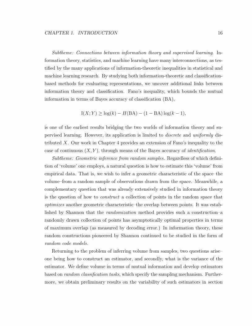
Subtheme: Connections between information theory and supervised learning. In-
formation theory, statistics, and machine learning have many interconnections, as tes-
tified by the many applications of information-theoretic inequalities in statistical and
machine learning research. By studying both information-theoretic and classification-
based methods for evaluating representations, we uncover additional links between
information theory and classification. Fano’s inequality, which bounds the mutual
information in terms of Bayes accuracy of classification (BA),
I(X;Y ) ≥ log(k)−H(BA)− (1− BA) log(k − 1),
is one of the earliest results bridging the two worlds of information theory and su-
pervised learning. However, its application is limited to discrete and uniformly dis-
tributed X. Our work in Chapter 4 provides an extension of Fano’s inequality to the
case of continuous (X, Y ), through means of the Bayes accuracy of identification.
Subtheme: Geometric inference from random samples. Regardless of which defini-
tion of ‘volume’ one employs, a natural question is how to estimate this ‘volume’ from
empirical data. That is, we wish to infer a geometric characteristic of the space–the
volume–from a random sample of observations drawn from the space. Meanwhile, a
complementary question that was already extensively studied in information theory
is the question of how to construct a collection of points in the random space that
optimizes another geometric characteristic–the overlap between points. It was estab-
lished by Shannon that the randomization method provides such a construction–a
randomly drawn collection of points has asymptotically optimal properties in terms
of maximum overlap (as measured by decoding error.) In information theory, these
random constructions pioneered by Shannon continued to be studied in the form of
random code models.
Returning to the problem of inferring volume from samples, two questions arise–
one being how to construct an estimator, and secondly, what is the variance of the
estimator. We define volume in terms of mutual information and develop estimators
based on random classification tasks, which specify the sampling mechanism. Further-
more, we obtain preliminary results on the variability of such estimators in section

CHAPTER 1. INTRODUCTION 17
2.4.4. We compare our results to existing results in information theory regarding
random code models.
Subtheme: Generalizability of experiments. Two of our motivations for studying
random classification tasks is (i) to evaluate representations, and (ii) as a model for
recognition problems. Yet a third application is for understanding the generalizabil-
ity of experiments that can be modelled as random classification tasks. For example,
many task-fMRI experiments can be modelled as random classification tasks, because
the stimuli sets used in the experiment are composed of arbitrary (‘random’) exem-
plars, and therefore the stimuli set used by one lab may differ from the stimuli set used
by another lab, even when they are presumably studying the same task. Intuitively,
holding all else fixed (such as the sample size per class), using larger and more diverse
stimuli sets should lead to better generalizability of results to the entire population of
stimuli. Our work on random classification–in particular, our variance bounds on the
classification accuracy in randomized classification tasks–provides a theoretical basis
for understanding how the results of a random classification task allow inference of
population parameters, such as the mutual information between the stimulus and the
response.
1.2.2 Organization
The rest of the thesis is organized as follows. The remaining sections in this chapter
deal with background material on supervised learning and information theory, as well
as the application of both to neuroscience, which forms a major motivation for the
current work. Chapter 2 introduces the concept of randomized classification, and also
establishes some variability bounds which will be used later in the development of
inference procedures. Chapter 3 studies the dependence of classification accuracy on
the label set size in randomized classification, and a practical method for predicting
the accuracy-versus-label set size curve from real data. Chapter 4 and 5 deal with the
applications of randomized classification to the estimation of mutual information in
continuous data: Chapter 4 derives a lower confidence bound for mutual information

CHAPTER 1. INTRODUCTION 18
under very weak assumptions, while Chapter 5 works within an asymptotic high-
dimensional framework which leads to a more powerful but less robust estimator
estimate of mutual information. We conclude the thesis with a discussion in Chapter
6.
1.3 Information and Discrimination
In studying the problem of evaluating representations, we make use of two closely
related frameworks: firstly, the multi-class classification framework from the statistics
and machine learning literature, and secondly, the concepts of information theory.
From a broader perspective, this is hardly unusual, since concepts such as entropy,
divergence, and mutual information are commonly applied in theoretical statistics and
machine learning. Furthermore, since information theory, theoretical statistics, and
machine learning are based on the same foundation of measure-theoretic probability
theory, one could go as far as to say that all three disciplines are subfields of applied
probability. However, while the three sub-fields may appear very similar from a
mathematical perspective, some differences arise if we examine the kinds of intuitions
and assumptions that are characteristic of the literature in each area.
At this point, we assume familiarity with the fundamentals of both supervised
learning and information theory. However, we refer the reader to section A.1 for a
review of supervised learning, and to section A.2 for a review of information theory.
In the rest of the chapter, we compare and contrast the kinds of problems studied
in supervised learning and information theory, and note what kind of cross-talk exists
between the two related fields, and what new developments could still arise by way
of a dialogue between supervised learning and information theory. One such new
development is the randomized classification model, since it is a very close analogue
of the random code model studied in information theory. Finally, we introduce the
identification task, a relatively new type of supervised learning task, which we propose
to utilize as a means for evaluating representations.

CHAPTER 1. INTRODUCTION 19
1.3.1 Comparisons
A common problem to statistics, information theory, and machine learning is the
inference of some unobserved quantity on the basis of observed quantities. In classi-
cal statistics, the problem is to infer an unknown parameter; in supervised learning,
the problem is to predict an unobserved label or response Y ; in information theory,
the problem is to decode a noisy message. Next, the metric for quantifying achiev-
able performance differs between the three disciplines. In classical statistics, one is
concerned with the variance of the estimated parameter, or equivalently, the Fisher in-
formation. In machine learning, one seeks to minimize (in expectation) a loss function
which measures the discrepancy between the prediction and the truth. In information
theory, one can measure the quality of the noisy channel (and therefore, the resulting
achievable accuracy) through the mutual information I(X;Y ) between the sender’s
encoded message X and the reciever’s recieved message Y . If we specialize within
machine learning to the study of classification, then we are concerned with accurate
discrimination of the input X according to labels Y . Similarly, if we specialize to the
problem of hypothesis testing within statistics, the problem is again to discriminate
between two (or more) different hypotheses regarding the data-generating mechanism.
Either natural or artificially intelligence recognition systems must rely on input
data that is informative of the optimal response if they are to achieve reasonable
discriminative accuracy. In natural environments, mammals rely on a combination of
visual, auditory, and tactile cues to recognize potential threats in the environment.
Mammalian brains integrate all of this sensory information in order to make more
rapid and reliable decisions. Generally, increased diversity and quality of the avail-
able sources of information will lead to more accurate recognition (say, of possible
environmental threats.)
This link between the information content of the input and the achievable discrim-
ination accuracy was first quantified by Claude Shannon via the concept of mutual
information. The mutual information I(X;Y ) quantifies the information content that
an input X holds about a target of interest, Y . For instance, in the case of facial
identification, the discrimination target Y is a label corresponding to the identity of
the person, and X is an image of the individual’s face. An image corrupted by noise

CHAPTER 1. INTRODUCTION 20
holds less information, and correspondingly leads to lower classification accuracies.
The discrmination problem that Shannon studied–the noisy-channel decoding prob-
lem, is extremely similar to the multi-class classification problem, but also features
some important differences. A side-by side comparison between the schematics of
multi-class classification and the noisy channel problem is displayed in Figure 1.5. We
will elaborate much further on the comparison illustrated in the figure, but for now,
one can note that both the multi-class classification problem and the noisy-channel
decoding problem involves the inference of a latent variable Y from an observation
X, where X is linked to Y through a conditional distribution FY . Here, Fy is the
conditional distribution of X given Y = y.
Therefore, we see that both the multi-class classification problem and the noisy
channel model present examples of discrimination problems where one must recover
some latent variable Y from observations X, where X is related to Y through the
family of conditional distributions FY . One difference is that while in multi-class
classification, FY is unknown and has to be inferred from data, in the noisy channel
model, the stochastic properties of the channel FY are usually assumed to be known.
A second difference is that in the noisy channel model, there is a choice in how to
specify the encoding function g(M), which affects subsequent performance. Finally,
in the broader research context, machine learning research has traditionally focused
on multi-class problems with relatively few classes, while information theory tends
to consider problems in asymptotic regimes where the number of possible messages
m is taken to infinity. These differences are perhaps sufficient to explain why little
overlap exists in the respective literatures between multi-class classification and the
noisy channel model.
However, an interesting development in the machine learning community has been
the application of multi-class classification to problems with increasingly large and
complex label sets. Consider the following timeline of representative papers in the
multi-class classification literature:
• Fisher’s Iris data set, Fisher 1936, K = 3 classes
• Letter recognition, Frey and Slate 1991, K = 26 classes

CHAPTER 1. INTRODUCTION 21
Multi-class classification Information Theory
label Y
distributionFY
observationX
classificationrule h(X)
estimate Y
message M
encoderg(M)
encodedmessage Y
noisychannel FY
observationX
decoderd(X)
estimateM
Figure 1.5: Comparing the discrimination tasks in multi-class classification and in-formation theory.

CHAPTER 1. INTRODUCTION 22
• Michalski’s soybean dataset, Mickalstd 1980, K = 15 classes
• The NIST handwritten digits data set, Grother 1995, K = 10 classes
• Phoneme recognition on the TIMIT datset, Clarkson and Moreno 1999, K = 39
classes
• Object categorization using Corel images, Duygulu et al. 2002 K = 371 classes
• Object categorization for ImageNet dataset, Deng et al. 2010, K = 10, 184
classes
• The 2nd Kaggle large-scale hierarchical text classification challenge (LSHTC),
Partalas et al. 2015, K = 325, 056
As we can see, in recent times we begin to see classification problems with extremely
large label sets. In such large-scale classification problems, or ‘extreme’ classification
problems, results for K → ∞ numbers of classes, like those found in information
theory, begin to look more applicable.
This work focuses on a particular intersection between multi-class classification
and information theory, which is the study of random classification tasks. In numerous
domains of applied mathematics, it has been found that systems with large numbers of
components can be modelled using randomized versions of those same systems, which
are more tractable to mathematical analysis: for example, studying the properties of
networks by studying random graphs in graph theory, or studying the performance
of combinatorial optimization algorithms for random problem instances. Similarly,
it makes sense to posit randomized models of multi-class discrimination problems.
Since information theorists were the first to study discrimination problems with large
number of classes, we find in the information theory literature a long tradition of
the study of random code models. This thesis is dedicated to the the study of the
analogue of random code models in the multi-class classification setting: models of
randomized classification, which we motivate and analyze in the next chapter.
CHAPTER 1. INTRODUCTION 23
1.3.2 Identification accuracy
The identification accuracy originated as a method for evaluating the quality of en-
coding models in neuroscience (Kay et al. 2008, Mitchell et al. 2008). However, it can
generally be applied to evaluate any regression model with a multivariate response
~Y . Furthermore, we argue that it can be an ideal method for evaluating the quality
of multivariate representations ~g( ~X) given a continuous multivariate response ~Y .
Suppose that we have pairs of vector-valued observations ( ~Xi, ~Yi)Ti=1, where the
features ~X are p-dimensional, and the response vectors ~Y are q-dimensional. For
instance, in the Kay et al. study of natural images, the features ~X are a basis of
10,921 Gabor filters coefficients for the presented images, and the response vectors ~Y
are a 3000-dimensional vector of activation coefficients from the visual cortex.
Step 1. Fitting the forward model
We would like to fit a linear2 multivariate regression model of the form
E[~Y | ~X = ~x] = ~xTB
where B is a p× q coefficient matrix. Data-splitting is used to partition the data into
a training and test set, so that the training set can be used to obtain an estimate of
the coefficient matrix, B, while the test set can be used to evaluate the quality of the
regression model.
To be specific, the T stimulus-response pairs ( ~X, ~Y ) are randomly partitioned into
a training set of size N and a test set of size M = T − N . Form the N × p data
matrix X tr by stacking the features of the N training set stimuli as row vectors,
and stack the corresponding responses as row vectors to form the N × q matrix Y tr.
Similarly, define X te as the N × p matrix of test stimuli and Y te as the N × q matrix
of corresponding test responses. Without loss of generality, let us suppose that the
indices i = 1, . . . ,M correspond to the test set, so that the test observations are
(~xi, ~yi)Mi=1.
2The discussion applies equally well to nonlinear regression models, but for expositional purposeswe focus on the special case of linear models.

CHAPTER 1. INTRODUCTION 24
Next, the coefficient B can be estimated from the training set data (X tr,Y tr)
using a variety of methods for regularized regression, for instance, the elastic net Zou
and Hastie 2005, where each column of B = (β1, . . . , βq) is estimated via
βi = argminβ||Y tri −X trβ||2 + λ1||β||1 + λ2||β||22,
where λ1 and λ2 are regularization parameters which can be chosen via cross-validation
(Hastie, Tibshirani, and Friedman 2009) separately for each column i.
After forming the estimated coefficient matrix B = (β1, . . . , βq), we estimate the
noise covariance Σ via a shrunken covariance estimate (Ledoit and Wolf 2004, Daniels
and Kass 2001) from the residuals,
Σ =1
N((1− λ)S + λDiag(S))
where
S = (Y tr −X trB)T (Y tr −X trB).
Step 2. Evaluating the forward model
A usual means of evaluating the linear model specified by the estimate B is to evaluate
the mean-squared error on the test set,
TMSE =1
M||Y te −X teB||2F ,
where a lower TMSE indicates a better model. Intuitively, the mean-squared error is
the average squared distance between an observation ~Y and its model prediction, Y
as illustrated in Figure 1.6(a).
However, an alternative criterion for evaluting the multivariate linear model was
proposed by Kay et al. 2008. In an identification task, as illustrated in Figure 1.6(b),
the model is first used to make predictions
yi = BT~xi

CHAPTER 1. INTRODUCTION 25
a b
Figure 1.6: Mean-squared error (a) versus identification accuracy (b) for evaluting amultivariate predictive model.
for all features {~xi}Mi=1 in the test set. Next, each of the observations ~yi in the test
set is assigned to the closest prediction {yj}Mj=1 within the test set. Here, ‘closest’ is
defined in terms of the the empirical Mahalanobis distance.
dΣ(~y, y) = (~y − y)T Σ−1(~y − y)
Finally, the M -point test identification accuracy is defined as the fraction of observa-
tions which are assigned to the correct prediction,
TIAM =1
M
M∑i=1
I(dΣ(~yi, yi) ≤ minj 6=i
dΣ(~yi, yj)).
Advantages of identification accuracy over MSE
A major reason why identification accuracy was adopted for fMRI studies is because
it provides an intuitive demonstration of how much information about the stimulus
~X is contained in the response ~Y , in a way that mean-squared error cannot. We
formalize this idea by explicitly showing how the empirical identification accuracy
can be used to obtain a lower bound of mutual information (Chapter 4). However,
some of the intuition can be demonstrated via the following toy example.
Suppose that the response ~Y and predictor ~X are both three-dimensional. The
predictor ~X is generated from a standard multivariate normal distribution, and then
~Y is generated according to the linear model
~Y = BT ~X + ε

CHAPTER 1. INTRODUCTION 26
where ε is multivariate normal
ε ∼ N(0, σ2I).
Now consider two different scenarios. In scenario 1, we have the model
~Y (1) = B(1)T ~X + ε
with
B(1) =
1 1 1
0 0 0
0 0 0
That is, the responses ~Y are only related to the first component of ~X. There is no
information in ~Y about the other two components of ~X, since ~Y is independent of
(X2, X3).
In scenario 2, we have the model
~Y (2) = B(2)T ~X + ε
with
B(2) =
1 0 0
0 1 0
0 0 1
Unlike in scenario 1, now each component Yi contains information about a different
component Xi of ~X. Therefore, ~Y contains information about all components of ~X,
Assume that a large amount of training data is available, so that there is practically
no estimation error for B. Suppose the test set consists of eight points, (~xi, ~yi)8i=1,
where
~x1 = (−1,−1,−1) ~x5 = (+1,−1,−1)
~x2 = (−1,−1,+1) ~x6 = (+1,−1,+1)
~x3 = (−1,+1,−1) ~x7 = (+1,+1,−1)
~x4 = (−1,+1,+1) ~x8 = (+1,+1,+1)

CHAPTER 1. INTRODUCTION 27
0 10 20 30 40 50
0.0
0.2
0.4
0.6
0.8
1.0
σ2
accu
racy
Scenario 1Scenario 2
Figure 1.7: Identification accuracies in toy example
Let us compare the two scenarios in terms of what happens when we evaluate
the model using mean-squared error. In both cases, the mean-squared error will be
approximately 3σ2. Therefore, MSE does not distinguish between a low-information
situation (Scenario 1) and a high-information situation (Scenario 2). Furthermore,
since the expected squared norm of Y is the same in both cases, the multivariate R2
similarly fails to distinguish the two scenarios.
Now consider the identification accuracy. In scenario 1, the fact that ~Y only con-
tains information about X1 means that it can only separate the two sets {~x1, . . . , ~x4}and {~x5, . . . , ~x8} from each other, but it cannot discriminate between stimuli ~x, ~x′
which have the same first component. It follows that regardless of how small σ2 is–
even in the noiseless case, the identification accuracy can be at most 14. On the other
hand, in scenario 2, it is clear that as σ2 goes to zero, that the accuracy increases to
1. In figure 1.7 we have computed the identification accuracy for the two scenarios
as a function of σ2. As we can see, for a large range of σ2 values, the identification
accuracy is greater in scenario 2 (reflecting greater information) than scenario 1.

CHAPTER 1. INTRODUCTION 28
Cross-validated identification accuracy
Notice that the procedure described earlier for computing the empirical identification
is non-deterministic, because of the randomness in data-splitting. Therefore, it is
extremely useful in practice to repeat the computation of identification accuracy for
multiple data splits of the same size, and then average the result.
Concretely, define the leave-k-out cross-validated estimate of identification accu-
racy as follows:
1. Let L be a large number of Monte Carlo trials. For i = 1, . . . , L, carry out
data-splitting to create a training set of size T −k, and a test set of size K. Let
TA(i) be the identification accuracy on the test set.
2. Define the cross-validated identification accuracy as the average over the L
quantities computed,
TAk,CV =1
L
L∑i=1
TA(i). (1.1)
We describe some applications of cross-validated identification accuracy to the
inference of mutual information in Chapters 4 and 5.

Chapter 2
Randomized classification
As we foreshadowed in the introduction, randomized classification is one of the three
methods we consider for evaluating representations. Two other applications of ran-
domized classification are (i) for providing a formalism for evaluting recognition sys-
tems, and (ii) for studying generalizability of certain classification-based experiments.
The application of recognition systems provides the most intuitive way of understand-
ing the randomized classification task; therefore, in this chapter, we begin with a
discussion in section 2.1 of recognition tasks, and within this context, motivate the
definition of a randomized classification task in section 2.2. We propose to use the
randomized classification task to model the problem of recognition, and to evalaute
performance via the average accuracy. Next, to put our ideas into practice, we need
ways to estimate the average accuracy from data, which we address in 2.3.
Meanwhile, the problem of generalizing classification experiments provides a nat-
ural motivation for studying the variance of classification accuracy within a random-
ized classification task, which we cover in section 2.4. Meanwhile, another one of the
methods we consider–the identification task, is closely connected with the random-
ized classification task. We discuss how our results in 2.4 can also be applied to the
identification accuracy.
29

CHAPTER 2. RANDOMIZED CLASSIFICATION 30
2.1 Recognition tasks
Human brains have a remarkable ability to recognize objects, faces, spoken syllables
and words, as well as written symbols or words. This recognition ability is essential
for everyday life. While researchers in artificial intelligence have attempted to meet
human benchmarks for these classical recognition tasks for the last few decades, only
very recent advances in machine learning, such as deep neural networks, have al-
lowed algorithmic recognition algorithms to approach or exceed human performance
(LeCun, Bengio, and Hinton 2015).
Within the statistics and machine learning literature, the usual formalism for
studying a recognition task is to pose it as a multi-class classification problem. One
delineates a finite set of distinct entities which are to be recognized and distinguished,
which is the label set Y . The input data is assumed to take the form of a finite-
dimensional real feature vector X ∈ Rp. Each input instance is associated with
exactly one true label Y ∈ Y . The solution to the classification problem takes the
form of an algorithmically implemented classification rule h that maps vectors X to
predicted labels Y ∈ Y . The classification rule can be constructed in a data-dependent
way: that is, one collects a number of labelled training observations (X1, Y1) which
is used to inform the construction of the classification rule h. The quality of the
classification rule h is measured by generalization accuracy
GA(h) = Pr[h(X) = Y ],
where the probability is defined with reference to the unknown population joint dis-
tribution1 of (X, Y ).
However, a limitation of the usual multi-class classification framework for studying
recognition problems is the assumption that the label set Y is finite and known in
advance. When considering human recognition capabilities, it is clear that this is not
1Note that GA(h) is a parameter which is defined with respect on a fixed classification rule hand the population of new observations; therefore, it cannot be observed directly. However, forany given classification rule h, even one constructed using data, it is possible to make inferenceson the unknown population-level accuracy GA(h), by using independent test data drawn from thepopulation.

CHAPTER 2. RANDOMIZED CLASSIFICATION 31
the case. Our ability to recognize faces is not limited to some pre-defined, fixed set
of faces; similarly with our ability to recognize objects in the environment. Humans
learn to recognize novel faces and objects on a daily basis. And, if artificial intelligence
is to fully match the human capability for recognition, it must also possess the ability
to add new categories of entities to its label set over time; however, at present, there
currently exists a void in the machine learning literature on the subject of the online
learning of new classes in the data.
The central theme of this thesis is the study of randomized classification, which
can be motivated as an extension of the classical multi-class classification framework
to accommodate the possibility of growing or infinite label sets Y . The basic approach
taken is to assume an infinite or even continuous label space Y , and then to study
the problem of classification on finite label sets S which are randomly sampled from
Y . This, therefore defines a randomized classification problem where the label set
is finite but may vary from instance to instance. One can then proceed to answer
questions about the variability of the performance due to randomness in the labels,
or how performance changes depending on the size of the random label set.
2.2 Randomized classification
2.2.1 Motivation
The formalism of classification is inadequate for studying many practical questions
related to the generalizability of the facial recognition system. Using test data, we es-
timate the generalization accuracy of a recognition system. However, these estimated
accuracies apply only to the particular collection of individuals {y(1), . . . , y(k)}. If we
were to add a new individual y(k+1) to the dataset, for instance, when photographs
are uploaded on Facebook containing a new user, this defines a totally new classifica-
tion problem because the expanded set of labels {y(1), . . . , y(k+1)} defines a different
response space than the old set of labels {y(1), . . . , y(k)}. Yet, these two classification
problems are clearly linked. To take another example, a client might want to run a
facial recognition system developed by lab A on their own database of individuals. In

CHAPTER 2. RANDOMIZED CLASSIFICATION 32
this case, there might be no overlap between the people in lab A’s database and the
people in the client’s database. And yet, the client might still expect the performance
figures reported by lab A to be informative of how well the recognition system will
do on their own database!
The question of how to link performance between two different but related clas-
sification tasks is an active area of research, known as transfer learning. But while
the two examples we just listed might be considered as examples of transfer learning
problems, the current literature on transfer learning, as far as we know, does not
study the problem of mutating label sets. Therefore, to address this new class of
questions about the generalizability of the recognition system, we need to formalize
our notions of (a) what constitutes a ‘recognition system’ which can be applied to
different classification problems, and (b) what assumptions about the problem, and
what assumptions about the classifiers used, allow one to infer performance in one
classification problem based on performance in another classification problem.
2.2.2 Setup
By ‘recognition system,’ we really mean a learning algorithm Λ which can take train-
ing data as input, and produce a classification rule for recognizing faces. While a
classification rule is bound to a specific label set, a learning algorithm can be applied
to datasets with arbitrary label sets, and be continually updated as new labels are
added to the label set. To ‘update’ a facial recognition system with new data means
to apply the learning algorithm to the updated database.
Now we can formalize what it means to generalize performance from one problem
to another. A classification problem P is specified by a label set Y , a predictor space
X , a joint distribution G on X ×Y , and a sampling scheme S for obtaining training
data (for example, to obtain n observations from G i.i.d.). The sampling scheme is
needed because we cannot say much about how the learning algorithm will perform
unless we know how much training data it is going to have. The generalization
accuracy (GA) of the algorithm Λ on the classification problem P = (Y ,X , G, S) is

CHAPTER 2. RANDOMIZED CLASSIFICATION 33
defined as the expected risk of the resulting classification rule h,
GAP (Λ) = E[GA(h)]
where h is produced by applying Λ to the training data, sampled by S. The expec-
tation is taken over the randomness in the generation of the training data.
At this point we have defined a general transfer learning problem: given two
different classification problems P1 = (Y1,X1, G1, S1) and P2 = (Y2,X2, G2, S2), what
can we say about the relationship between GAP1(Λ) and GAP2(Λ)? Not much, unless
we make many more assumptions about how P1 and P2 are linked.
The basic approach we will take is to assume that both P1 and P2 have been
generated randomly via a common mechanism. In the original motivating context
of facial recognition, this is to say that two different label sets Y1 and Y2 are linked
because they both belong to a common population of labels Y , i.e., the population of
all possible humans, and to further assume that both have been sampled, in the same
manner, from Y .
The study of how to make inferences about the risk in P2 given information about
the performance achieved in P1, granted a set of assumptions on how P1 and P2
have been randomly generated (and are thereby linked through shared randomization
mechanisms) forms the basis of the subject of randomized classification.
As we noted in the introduction, the problem of randomized classification has
a close ancestor in the study of random code models in information theory. There,
the problem is to understand the decoding performance (the analogue to risk) of a
encoding/decoding system P which has a randomized code space Y . Where random
code models have a random codebook which is a sample over a distribution of all
possible codes, randomized classification problems have a random label set that is a
sample of a larger label space. However, the results we obtain for randomized classi-
fication are more general in nature than the existing results availible for random code
models, because work on random codes is generally limited to asymptotic settings,
whereas we obtain finite-k results, and because random code models assume a specific
product-distribution structure on (X, Y ) which is not appropriate for classification

CHAPTER 2. RANDOMIZED CLASSIFICATION 34
problems.
2.2.3 Assumptions
The randomized classification model we study has the following features. We assume
that there exists an infinite (or even continuous) label space Y and a feature space
X ∈ Rp. Let P(X ) be the space of probability distributions over X . For each label
y ∈ Y , there exists a distribution of features Fy ∈ P(X ). That is to say, that for a
feature-label pair (X, Y ), that the conditional distribution of X given Y = y is given
by Fy.
A random classification task P can be generated as follows. The label set S =
{Y (1), . . . , Y (k)} is generated by drawing labels Y (1), . . . , Y (k) i.i.d. from π. The joint
distribution G of pairs (X, Y ) is uniquely specified by the two conditions that (i) the
marginal distribution of Y is uniform over Y , and (ii) the conditional distribution of X
given Y = Y (i) is FY (i) . We sample both a training set and a test set. The training set
is obtained by sampling r1 observations X(i)j,train i.i.d. from FY (i) for j = 1, . . . , r1 and
i = 1, . . . , k. The test set is likewise obtained by sampling r2 observations X(i)j i.i.d.
from FY (i) for j = 1, . . . , r2. For notational convenience, we represent the training set
as the set of empirical distributions {FY (i)}ki=1 where
FY (i) =1
r1
r1∑j=1
δX
(i)j,train
.
Figure 2.1 illustrates the sampling scheme for generating the training set.
Our analysis will also rely on a property of the classifier. We do not want the
classifier to rely too strongly on complicated interactions between the labels in the set.
We therefore propose the following property of marginal separability for classification
models:
Definition 2.2.1 1. The classification rule h is called a marginal rule if
h(x) = argmaxy∈Smy(x),

CHAPTER 2. RANDOMIZED CLASSIFICATION 35
Figure 2.1: Training set
where each function my maps X to R.
2. Define a marginal modelM as a mapping from empirical distributions to margin
functions,
M : P(X )→ R(X )
where R(X ) is the space of real-valued functions on X . That is, if we write
my =M(Fy),
then my(x) is a real-valued function with domain X .
3. A classifier that produces marginal classification rules
h(x) = argmaxy∈Smy(x),
by use of a marginal model, i.e. such that my = M(Fy) for some marginal
model M, is called a marginal classifier.
In words, a marginal classification rule produces a margin, or score2, for each label,
and chooses the label with the highest margin. The marginal model converts empirical
distributions Fy over X into the margin function my. The marginal property allows
2The margin my(x) is also called a discriminant function in the statistics literature.
CHAPTER 2. RANDOMIZED CLASSIFICATION 36
us to prove strong results about the accuracy of the classifier under i.i.d. sampling
assumptions.
Comments:
1. The marginal model includes several popular classifiers. A primary example for
a marginal model is the estimated Bayes classifier. Let fy be a density estimate
obtained from the empirical distribution Fy. Then, we can use the estimated
densities of each class to produce the margin functions:
mEBy (x) = log(fy(x)).
The resulting empirical approximation for the Bayes classifier (further assuming
a uniform prior π) would be
fEB(x) = argmaxy∈S(mEBy (x)).
2. Both the Quadratic Discriminant Analysis and the naive Bayes classifiers can
be seen as specific instances of an estimated Bayes classifier 3. For QDA, the
margin function is given by
mQDAy (x) = −(x− µ(Fy))
TΣ(Fy)−1(x− µ(Fy))− log det(Σ(Fy)),
where µ(F ) =∫ydF (y) and Σ(F ) =
∫(y − µ(F ))(y − µ(F ))TdF (y). In Naive
Bayes, the margin function is
mNBy (x) =
n∑i=1
log fy,i(x),
where fy,i is a density estimate for the i-th component of Fy.
3. There are many classifiers which do not satisfy the marginal property, such as
3QDA is the special case of the estimated Bayes classifier when fy is obtained as the multivariateGaussian density with mean and covariance parameters estimated from the data. Naive Bayes is theestimated Bayes classifier when fy is obtained as the product of estimated componentwise marginaldistributions of p(xi|y)

CHAPTER 2. RANDOMIZED CLASSIFICATION 37
multinomial logistic regression, multilayer neural networks, decision trees, and
k-nearest neighbors.
The operation of a marginal classifier is illustrated in figure 2.2. Since a marginal
classifier is specified entirely by its marginal model M, we will take the notational
convention of referring to a marginal classifier as M.
Figure 2.2: Classification rule
We would like to identify the sources of randomness in evaluating a classifier. First,
there is the specific choice of k classes for the label set. Second, there is randomness
in training the classifier for these classes, which comes from the use of a finite training
set. Third, there is the randomness in the estimated risk when testing the classifier
on a test set.
If we fix a particular realization of the random label set S = {y(1), . . . , y(k)} as
well as the training set {Fy(i)}ki=1, then the classifier h(x) is fixed, and only the third
source of randomness (in test risk) applies. However, the true generalization accuracy

CHAPTER 2. RANDOMIZED CLASSIFICATION 38
of the classifier is deterministic4:
GA(h) = Pr[Y = h(X)|S, {Fy(i)}ki=1]
=1
k
k∑i=1
Pr[my(i)(X(i)) = max
jmy(j)(X
(i))|S, {Fy(i)}ki=1].
=1
k
k∑i=1
∫XI(my(i)(x) = max
jmy(j)(x))dFy(i)(x),
where the probabilities are evalutated with respect to the joint distribution of Y ∼Unif(S) and X(i) ∼ FY (i) for i = 1, . . . , k; also recalling that my(i)(x)
def= M(Fy(i))(x)
is the margin function obtained from the training data of the ith class.
If we fix a particular realization of the random label set S = {y(1), . . . , y(k)}, then
we can define the (generalization) accuracy specific to that label set. However, the
training data {Fy(i)}ki=1 will be random. Let us denote the distribution of the empirical
distribution Fy constructed from sample size r as Πy,r. The accuracy of the classifier
M on label set S is given by
GAS(M) = Pr[Y = h(X)]
=1
k
k∑i=1
∫I(M(Fy(i))(x) = max
jM(Fy(j))(x))dFy(i)(x)
k∏`=1
dΠy(`),r1(Fy(`))
where the probability is taken with respect to the joint distribution of Y ∼ Unif(S), Fy(i) ∼Πy(i),r1 . The calculation of the accuracy (for fixed label set S) is illustrated in figure
2.3.
Finally, suppose we do not fix any of the random quantities in the classification
task P , and merely specify k, the number of classes, and r1, the number of repeats
in the training set. Then the k-class, r-repeat average generalization accuracy of a
4Although h is data-dependent and therefore random, for a fixed h, the generalization accuracyis a deterministic parameter which depends on h and the population.
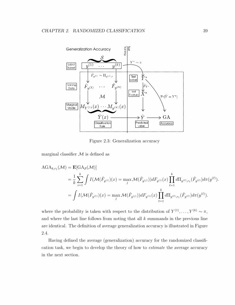
CHAPTER 2. RANDOMIZED CLASSIFICATION 39
Figure 2.3: Generalization accuracy
marginal classifier M is defined as
AGAk,r1(M) = E[GAS(M)]
=1
k
k∑i=1
∫I(M(Fy(i))(x) = max
jM(Fy(j)))dFy(i)(x)
k∏`=1
dΠy(`),r1(Fy(`))dπ(y(`)).
=
∫I(M(Fy(1))(x) = max
jM(Fy(j)))dFy(1)(x)
k∏`=1
dΠy(`),r1(Fy(`))dπ(y(`)).
where the probability is taken with respect to the distribution of Y (1), . . . , Y (k) ∼ π,
and where the last line follows from noting that all k summands in the previous line
are identical. The definition of average generalization accuracy is illustrated in Figure
2.4.
Having defined the average (generalization) accuracy for the randomized classifi-
cation task, we begin to develop the theory of how to estimate the average accuracy
in the next section.

CHAPTER 2. RANDOMIZED CLASSIFICATION 40
Figure 2.4: Average generalization accuracy
2.3 Estimation of average accuracy
Suppose we have training and test data for a classification task P1 with k1 classes, r1-
repeat training data and r2-repeat test data. That is, we have label set S1 = {y(i)}k1i=1,
as well as training sample Fy(i) and test sample (x(i)1 , . . . , x
(i)r2 ) for i = 1, . . . , k1. How
can we estimate the k, r-average accuracy of a marginal classifier M for arbitrary k
and r?
Let us start with the case k = k1 and r = r1. Then the answer is simple: construct
the classification rule h using marginal model M from the training data. Then the
test accuracy of h is an unbiased estimator of AGAk,r.
This follows from definition. Observe that AGAk1,r1 is the expected prediction
risk for the classification rule h for a randomized classification problem P with k1
classes and r1-repeat training data. Of course, the classification task P1 that we have
been given is a random draw from the desired distribution of random classification
problems. Therefore, the prediction risk of h constructed from P1 is unbiased for

CHAPTER 2. RANDOMIZED CLASSIFICATION 41
AGAk1,r1 , and since test accuracy is unbiased for generalization accuracy, it follows
that the test accuracy of h is an unbiased estimator of AGAk,r, as we claimed.
In following sections, we consider more complicated cases where k1 6= k. However,
before proceeding, let us first review the procedure for computing the test accuracy.
For any given test observation x(i)j , we obtain the predicted label y
(i)j by computing
the margin for each class,
Mi,j,` =M(Fy(`))(x(i)j ) = my(`)(x
(j)i ),
for ` = 1, . . . , k1, and by finding the class with the highest margin Mi,j,`,
y(i)j = y(argmax`Mi,j,`).
The test accuracy is the fraction of correct classification over test observations,
TA =1
r2k1
k1∑i=1
r2∑j=1
I(y(i)j = y(i)). (2.1)
For each test observation, define the ranks of the margins by
Ri,j,` =∑m 6=`
I{Mi,j,` ≥Mi,j,m}.
Therefore, y(i)j is equal to y(i) if and only if Ri,j,i = k1. Thus, an equivalent expression
for test accuracy is
TA =1
r2k1
k1∑i=1
r2∑j=1
I{Riji = k1}. (2.2)
2.3.1 Subsampling method
Next, let us consider the case where k < k1 and r = r1. Define a classification problem
P2 with label set S2 obtained by sampling k labels uniformly without replacement
from S1. Let the training and test data for P2 be obtained by taking the training

CHAPTER 2. RANDOMIZED CLASSIFICATION 42
data and test data from P1 belonging to labels in S1. It follows that P2 is a ran-
domized classification task with k labels, r1-repeat training data and r2-repeat test
data. Therefore, by the previous argument, the test accuracy for a classification rule
h constructed using the training data in P2 provides an unbiased estimate of AGAk,r1 .
However, we can get a much better unbiased estimate of AGAk,r1 by averaging
over the randomization of S2. Naıvely, this requires us to train and evaluate(k1k
)classification rules. However, due to the special structure of marginal classifiers, we do
the computation in the same order of computation as evaluating a single classification
rule (assuming that the computational bottleneck is in training the classifier.)
This is because the rank Riji of the correct label, i, for the x(i)j allows us to
determine how many subsets S2 will result in a correct classification. For example
x(i)j , there are Riji− 1 labels with a lower margin than the correct label i. Therefore,
as long as one of the classes in S2 is i, and the other k − 1 labels are from the set
of Riji − 1 labels with lower margin than i, the classification of x(i)j will be correct.
This implies that there are(Riji−1k−1
)such subsets S2 where x
(i)j is classified correctly,
and therefore
AverageTAk,r1 =1(k1k
) 1
r2k
k1∑i=1
r2∑j=1
(Riji − 1
k − 1
). (2.3)
2.3.2 Extrapolation
A much more challenging case is when k2 > k1: that is, we want to predict the
performance of the classification model in a setting with more labels than we currently
see in the training set. This is the subject of Chapter 3.
2.3.3 Variance bounds
By now we have developed unbiased estimators for average generalization accuracy
in the special case k ≤ k1, and the following chapter will present methods for the
more difficult case k > k1. However, to get useful inference statements, we also have
to understand the variance of these estimators. For the large part, this is still work-
in-progress. However, some first steps towards addressing this problem are described

CHAPTER 2. RANDOMIZED CLASSIFICATION 43
in the next section.
2.4 Reproducibility and Average Bayes accuracy
2.4.1 Motivation
In task fMRI experiments, one typically obtains data of the form (~xi, yi), where
~xi are activity patterns obtained from the fMRI scan for a region of interest, and
yi are categories for tasks. The labels yi are limited to a discrete label set S =
{y(1), . . . , y(k)}. Data-splitting is used to obtain a test accuracy TA for predicting
y from ~x. The test accuracy is then interpreted as evidence for the specialization
of that region of interest for the task at hand: a high accuracy suggests that the
region is specialized for the task, while a low accuracy suggests that the region is not
specialized for the task.
However, a limitation of this approach is the poor reproducibility of the test
accuracy TA. Besides the dependence of TA on the particular subject participating in
the experiment, the randomness in sampling training and test data, and the classifier
used, there is an even more fundamental issue in that the classification task is often
inconsistent from lab to lab. That is because the task exemplars–that is, the set of
labels {y(i)}ki=1, may be arbitrarily specified, and therefore even ignoring the effect of
subject, sampling of the data, and classifier, the generalization accuracy depends on
an arbitrary choice of exemplars.
On the other hand, fixing in advance the set of exemplars {y(i)}ki=1 is also not
a satisfactory solution, since the objective of the experiment is to understand the
general relation between the task and the region of interest, and not the relationship
between a particular set of task exemplars {y(i)}ki=1 and the region of interest.
Randomized classification provides a solution for addressing both the variability
in estimation target and generalization to the population, as long as one can justify
the assumption that the labels {y(i)}ki=1 are a random sample from some population
of task exemplars π. While the generalization accuracy GA for any particular, fixed
set of exemplars is not a population parameter, the average generalization accuracy

CHAPTER 2. RANDOMIZED CLASSIFICATION 44
AGA is defined with reference to a population, albeit also dependent on a specific
classifier and sampling scheme. Meanwhile, the limitations on reproducibility due to
differing choices of labels sets can be understood based on the variability properties
of GA.
However, one can argue that randomized classification does not go far enough to
ensure generalizability of results, because AGA still depends on the sampling scheme
(the amount of training data) and the choice of classifier, which are both arbitrary
experimental choices. Therefore, our proposal is to treat the average Bayes accuracy
as the estimation target of interest. The average Bayes accuracy is defined indepen-
dently of the classifier and sampling scheme, and we will develop tools for inferring
probabilistic lower bounds (lower confidence bounds) of the average Bayes accuracy
in this section.
2.4.2 Setup
The generalization accuracy of any classification rule is upper-bounded by the ac-
curacy of the optimal classification rule, or Bayes rule. That is, one can define the
Bayes accuracy as
BA = suph
GA(h).
And due to Bayes’ theorem, the optimal classification rule h∗ which achieves the
Bayes accuracy can be given explicitly: it is the maximum a posteriori (MAP) rule
h∗(x) = argmaxki=1 p(x|y(i)).
Of course, it is not possible to construct this rule in practice since the joint distribution
is unknown. Instead, a reasonable approach is to try a variety of classifiers, producing
rules h1, . . . , hm, and taking the best generalization accuracy as an estimate of the
Bayes accuracy.
Now consider a randomized classification task where the labels {Y (1), . . . , Y (k)}are drawn iid from a population π, and where the observations X for label Y are
drawn from the conditional distribution FY . In this case, the Bayes accuracy is a

CHAPTER 2. RANDOMIZED CLASSIFICATION 45
random variable depending on the label set, since
BA(y(1), . . . , y(k)) =1
k
k∑i=1
Pr[argmaxki=1 p(X(i)|y(i)) = i].
where the probabilities inside the sum are taken with respect to the distribution of
X(i) ∼ Fy(i) for each i = 1, . . . , k. The k-class Average Bayes accuracy is defined as
the average Bayes accuracy,
ABAk = E[BA(Y (1), . . . , Y (k))]
where the expectation is taken over the joint distribution of {Y (1), . . . , Y (k)}.
2.4.3 Identities
The following theorem gives a convenient formula for computing ABAk.
Theorem 2.4.1 Suppose (X, Y ) have a joint distribution with a density p(x, y), with
a marginal density π(y). Then for a randomized classification task with {Y (1), . . . , Y (k)}are drawn iid from π, the k-class average Bayes accuracy can be computed as
ABAk[p(x, y)] =1
k
∫ [ k∏i=1
π(yi)dyi
]∫dxmax
ip(x|yi).
Proof. Write
ABAk[p(x, y)] = E[BA(Y (1), . . . , Y (k))]
=1
k
∫π(y1) . . . π(yk)
k∑i=1
I{argmaxki=1 p(x|yi) = i}p(x|yi)dxdy1 . . . dyk
=1
k
∫π(y1) . . . π(yk)p(x|yargmaxki=1 p(x|yi))dy1 . . . dykdx.
=1
k
∫π(y1) . . . π(yk)
kmaxi=1
p(x|yi)dy1 . . . dykdx.

CHAPTER 2. RANDOMIZED CLASSIFICATION 46
2.4.4 Variability of Bayes Accuracy
By definition, BAk = BA(X1, ..., Xk) is already an unbiased estimator of ABAk.
However, to get confidence intervals for ABAk, we also need to know the variability
of BAk.
We have the following upper bound on the variability.
Theorem 2.4.2 For a randomized classification task with {Y (1), . . . , Y (k)} are drawn
iid from π, the variability of the Bayes accuracy can be bounded as
Var[BA(Y (1), ..., Y (k))] ≤ 1
4k.
Proof. According to the Efron-Stein inequality (Efron and Stein 1981),
Var[BA(Y (1), ..., Y (k))] ≤k∑i=1
E[Var[BA|Y (1), ..., Y (i−1), Y (i+1), ..., Y (k)]].
which is the same as
Var[BA(Y (1), ..., Y (k))] ≤ kE[Var[BA|Y (1), ..., Y (k−1)]].
The term Var[BA|Y (1), ..., Y (k−1)] is the variance of BA(Y (1), ..., Y (k)) conditional
on fixing the first k − 1 curves p(x|y(1)), ..., p(x|y(k−1)) and allowing the final curve
p(x|Y (k)) to vary randomly.
Note the following trivial results
−p(x|y(k)) +k
maxi=1
p(x|y(i)) ≤ k−1maxi=1
p(x|y(i)) ≤ kmaxi=1
p(x|y(i)).
This implies
BA(Y (1), ..., Y (k))− 1
k≤ k − 1
kBA(Y (1), ..., Y (k−1)) ≤ BA(Y (1), ..., Y (k)).
i.e. conditional on (Y (1), ..., Y (k−1)), BAk is supported on an interval of size 1/k.

CHAPTER 2. RANDOMIZED CLASSIFICATION 47
Therefore,
Var[BA|Y (1), ..., Y (k−1)] ≤ 1
4k2
since 14c2
is the maximal variance for any r.v. with support of length c. �
2.4.5 Inference of average Bayes accuracy
Recall the procedure used to estimate generalization error: by applying data-splitting,
one creates a training set consisting of r1 repeats per class, and a test set consisting
of the remaining r2 = r − r1 repeats. One inputs the training data into the classifier
to obtain the classification rule f , and computes the test accuracy,
GA =1
kr2
k∑i=1
r∑j=r1+1
I(f(x(i)j ) 6= i).
Since kr2GA is a sum of independent binary random variables, from Hoeffding’s
inequality, we have
Pr[GA > GA +t
kr2
] ≤ 2e−2kr2t2 .
Therefore,
GAα = GA−
√− log(α/2)
2kr2
is a (1− α) lower confidence bound for GA(f). But, since
GA(f) ≤ BA(y(1), . . . , y(k)),
it follows that GAα is also a (1− α) lower confidence bound for BA(x(1), . . . , x(k)).
Next, consider the variance bound for BA. From Chebyshev’s inequality,
Pr[|BA(Y (1), . . . , Y (k))− ABAk| >1√4αk
] ≤ α.
Combining these facts, we get the following result.

CHAPTER 2. RANDOMIZED CLASSIFICATION 48
Theorem 2.4.3 The following is a (1− α) lower confidence bound for ABAk:
ABAk = GA−
√− log(α/4)
2kr2
− 1√2αk
.
That is,
Pr[ABAk > ABAk] ≤ α.
Proof. Suppose that both BA(Y (1), . . . , Y (k)) ≤ ABAk + 1√2αk
and GAα/2 ≤ GA.
Then it follows that
GAα/2 ≤ BA(Y (1), . . . , Y (k)) ≤ ABAk +1√2αk
and hence
ABAk = GAα/2 −1√2αk
≤ ABAk.
Therefore, in order for a type I error to occur, either BA(Y (1), . . . , Y (k)) > ABAk +1√2αk
or GAα/2 > GA. But each of these two events has probability of at most α/2,
hence the union of the probabilities is at most α. �
2.4.6 Implications for reproducibility
Returning to the original problem of experimental reproducibility or generalizability
to a larger population under the assuption that the task exemplars have been drawn
from a population. It follows from our analysis that both reproducibility and genral-
izability are assured if experimental parameters enable inference of a lower confidence
bound ABAk which is close to the true average Bayes accuracy. This would require
two conditions:
1. The training data is sufficiently large, and the classifier is chosen so that the
generalization accuracy is close to the Bayes accuracy.
2. The number of classes k is sufficiently large so that the Bayes accuracy BA(Y (1), . . . , Y (k))
is close to the average Bayes accuracy.

CHAPTER 2. RANDOMIZED CLASSIFICATION 49
Under those two conditions, the lower confidence bounds ABAk have a distribution
which is concentrated close to the true population parameter ABAk, which ensures
both reproducibility (in the estimates produced by two realizations of the same ran-
domized classification task) and generalizability to the population parameter ABA.
Our analysis of the variance of BAk gives an easy criterion for ensuring that k
is large enough, since k needs to be inversely proportional to the desired variance.
However, we have not developed methods for checking condition 1. In practice, when a
large number of different classifiers achieve similar accuracies, and when performance
is not particularly affected by training on a fractional subsample of the training data,
this can be heuristically taken as evidence that the generalization accuracy is close
to Bayes accuracy. However, it remains to theoretically characterize the assumptions
that make this possible (e.g. smoothness of the model, low signal-to-noise ratio) and
to develop formal tests for convergence to Bayes accuracy.
2.4.7 Application to identification task
In the same way that average Bayes accuracy provides an upper bound for the average
generalization error in the randomized classification task, the average Bayes accuracy
can also bound the expected cross-validated identification accuracy (1.1).
This is clear if we define a generalized identification task, which is constructed as
follows:
Generalized identification task
1. Draw ~X1, . . . , ~Xk from the marginal distribution of ~X.
2. Draw index J uniformly from {1, . . . , k}.
3. Generate ~Y from the conditional distribution p(~y| ~X = ~Xj).
4. Let g be a function which takes a response vector ~Y and k feature vectors
~X1, . . . , ~Xk and outputs an index in {1, . . . , k}
g : Y × X k → {1, . . . , k}.

CHAPTER 2. RANDOMIZED CLASSIFICATION 50
Define the identification generalization accuracy of g as
Pr[g(~Y ; ~X1, . . . , ~Xk) = J ]
under the above setup.
We will now claim the following. Claim 1: the identification task introduced in
section 1.3.2 is a special case of the generalized identification task. Claim 2: one can
define a randomized classification task such that the k-class average Bayes accuracy
is an upper bound of the identification generalization accuracy.
Claim 1 can be argued as follows. In the identification task introduced in section
1.3.2, when we fix a training set, the expected test identification accuracy is equivalent
to the identification generalization accuracy of a rule g, which can be writen as
g(~Y ; ~X1, . . . , ~Xk) = argminj(~Y − f( ~Xj))T Σ−1(~Y − f( ~Xj)).
where f(~x) is the estimate of the regression function E[~Y | ~X = ~x], and Σ is the
estimated covariance matrix of the noise.
Claim 2 follows because the Bayes identification rule,
g(~Y ; ~X1, . . . , ~Xk) = argmaxjp(~Y | ~X = ~x)
maximizes the identification generalization accuracy over all functions g. But now
consider a randomized classification task where ~X are the labels, and ~Y are the feature
vectors (note that this is the reverse of the convention previously used in this chapter.)
Then we see that the Bayes identification rule g is also the Bayes classification rule
for the label set { ~X1, . . . , ~Xk}.Since the average Bayes accuracy is an upper-bound for the expected identification
accuracy over any training-test split, it follows that ABAk is also an upper bound for
the expected CV-identification accuracy: that is,
ABAk ≥ E[TAk,CV ] (2.4)

CHAPTER 2. RANDOMIZED CLASSIFICATION 51
for TAk,CV as defined in (1.1).
We use this fact in Chapters 4 and 5 to link identification accuracy to mutual
information via the average Bayes accuracy.
Chapter 3
Extrapolating average accuracy
3.1 Introduction
In this chapter, we continue the discussion of Chapter 2, but focus specifically on
the question of how to estimate the k-class average accuracy, AGAk,r1 , based on data
from a problem P1 with k1 < k classes, and r1-repeat training data. This problem of
prediction extrapolation is especially interesting for a number of applied problems.
• Example 1: A researcher develops a classifier for the purpose of labelling images
in 10,000 classes. However, for a pilot study, her resources are sufficient to tag
only a smaller subset of these classes, perhaps 100. Can she estimate how well
the algorithm will work on the full set of classes based on an initial ”pilot”
subsample of class labels?
• Example 2: A neuroscientist is interested in how well the brain activity in
various regions of the brain can discriminate between different classes of stimuli.
Kay et al. 2008 obtained fMRI brain scans which record how a single subject’s
visual cortex responds to natural images. They wanted to know how well the
brain signals could discriminate between different images. For a set of 1750
photographs, they constructed a classifier which achieved over 0.75 accuracy of
classification. Based on exponential extrapolation, they estimate that it would
take on the order of 109.5 classes before the accuracy of the model drops below
52

CHAPTER 3. EXTRAPOLATING AVERAGE ACCURACY 53
0.10! A theory of performance extrapolation could be useful for the purpose of
making such extrapolations in a more principled way.
• The stories just described can be viewed as a metaphor for typical paradigm of
machine learning research, where academic researchers, working under limited
resources, develop novel algorithms and apply them to relatively small-scale
datasets. Those same algorithms may then be adopted by companies and ap-
plied to much larger datasets with many more classes. In this scenario, it would
be convenient if one could simply assume that performance on the smaller-scale
classification problems was highly representative of performance on larger-scale
problems.
Previous works have shown that generalizing from a small set of classes to a
larger one is not straightforward. In a paper titled “What does classifying more than
10,000 Image Categories Tell Us,” Deng and co-authors compared the performance of
four different classifiers on three different scales: a small-scale (1,000-class) problem,
medium-scale (7,404-class) problem, and large-scale (10,184-class) problem (all from
ImageNet.) They found that while the nearest-neighbor classifier outperformed the
support vector machine classifier (SVM) in the small and medium scale, the ranking
switched in the large scale, where the SVM classifier outperformed nearest-neighbor.
As they write in their conclusion, “we cannot always rely on experiments on small
datasets to predict performance at large scale.” Theory for performance extrapola-
tion may therefore reveal models with bad scaling properties in the pilot stages of
development.
However, in order to formally develop a method for extrapolating performance,
it is necessary to specify the model for how the small-scale problem is related to
the larger-scale problem. The framework of randomized classification introduced in
Chapter 2 is one possible choice for such a model: the small-scale problem and large-
scale problem are linked by having classes drawn from the same population.
The rest of the chapter is organized as follows. We begin by continuing to analyze
the average accuracy AGAk,r, which results in an explicit formula for the average
accuracy. The formula reveals that all of the information needed to compute the

CHAPTER 3. EXTRAPOLATING AVERAGE ACCURACY 54
average accuracy is contained in a one-dimensional function D(u), and therefore that
estimation of the average accuracy can be accomplished via estimation of the unknown
function D(u). This allows the development of a class of unbiased estimators of
D(u), presented in section 3.3 given the assumption of a known parametric form
for D(u). We demonstrate our method to a face-recognition example in section 3.4.
Additionally, in Chapter 5 we compare the estimator to an alternative, information-
theory based estimator in simulated and real-data examples.
3.2 Analysis of average risk
The result of our analysis is to expose the average accuracy AGAk,r as the weighted
average of a function D(u), where D(u) is independent of k, and where k only changes
the weighting. The result is stated as follows.
Theorem 3.2.1 Suppose π, {Fy}y∈Y and marginal classifier F satisfy the tie-breaking
condition. Then, under the definitions (3.2) and (3.5), we have
AGAk,r = 1− (k − 1)
∫D(u)uk−2du. (3.1)
The tie-breaking condition referred in the theorem is defined as follows.
• Tie-breaking condition: for all x ∈ X , M(FY )(x) = M(FY ′)(x) with zero
probability for Y, Y ′ independently drawn from π.
The tie-breaking condition is a technical assumption which allows us to neglect the
specification of a tie-breaking rule in the case that margins are tied. In practice, one
can simply break ties randomly, which is mathematically equivalent to adding a small
amount of random noise ε to the function M.
As we can see from Figure 2.4, the average accuracy is obtained by averaging over
four randomizations:
A1. Drawing the label subset S.
A2. Drawing the training dataset, FY (1) , . . . , FY k .

CHAPTER 3. EXTRAPOLATING AVERAGE ACCURACY 55
A3. Drawing Y ∗ uniformly at random from S.
A4. Drawing X∗ from FY ∗ .
Our strategy is to analyze the average accuracy by means of conditioning on the
true label and its training sample, (y∗, Fy∗), and the test feature x∗ while averaging
over all the other random variables. Define the conditional accuracy CondAcck((y∗, Fy∗), x
∗)
as
CondAcck((y∗, Fy∗), x
∗) = Pr[argmaxy∈SM(Fy)(X∗) = Y ∗|Y ∗ = y∗, X∗ = x∗, FY ∗ = Fy∗ ].
Figure 3.1 illustrates the variables which are fixed under conditioning and the variables
which are randomized. Compare to figure 2.4.
Without loss of generality, we can write the label subset S = {Y ∗, Y (1), . . . , Y (k−1)}.Note that due to independence, Y (1), . . . , Y (k−1) are still i.i.d. from π even condition-
ing on Y ∗ = y∗. Therefore, the conditional risk can be obtained via the following
alternative order of randomizations:
C0. Fix y∗, Fy∗ , and x∗. Note that My∗(x∗) =M(Fy∗)(x
∗) is also fixed.
C1. Draw the incorrect labels Y (1), . . . , Y (k−1) i.i.d. from π. (Note that Y (i) 6= y∗
with probability 1 due to the continuity assumptions on Y and π.)
C2. Draw the training samples for the incorrect labels FY (1) , . . . , FY (k−1) . This de-
termines
Y = argmaxy∈SMy(x∗)
and hence, whether or not the classification is correct for (x∗, y∗)
Compared to four randomization steps for the average risk, we have essentially con-
ditioned on steps A3 and A4 and randomized over steps A1 and A2.
Now, in order to analyze the k-class behavior of the conditional accuracy, we begin
by considering the two-class situation.
In the two-class situation, we have a true label y∗, a training sample Fy∗ , and one
incorrect label, Y . In this case, we obtain the margin functions for both classes from

CHAPTER 3. EXTRAPOLATING AVERAGE ACCURACY 56
Figure 3.1: Conditional accuracy
the training data,
My∗ =M(Fy∗),
for the correct label, and
MY =M(FY )
for the random incorrect label. The classification is correct if and only if
My∗(x∗) ≥MY (x∗),
that is, if the score of the incorrect class is larger than the score of the correct class
for observation x∗.
Define the U-function Ux∗(y∗, Fy∗) as the conditional accuracy (the probability of
correct classification) in the two-class case. Since we are fixing x∗ and (y∗, Fy∗), the

CHAPTER 3. EXTRAPOLATING AVERAGE ACCURACY 57
probability of correct classification is obtained by taking an expectation:
Ux∗(y∗, Fy∗) = Pr[My∗(x
∗) >M(FY )(x∗)] (3.2)
=
∫Y×PY
I{My∗(x∗) >M(Fy)(x
∗)}dΠy,r(Fy)dπ(y). (3.3)
Recall that Πy,r is the distribution of Fy, where Fy is the empirical distribution of
a sample of size r from label y (that is, Πy,r is a distribution over distributions), as
we defined in section 2.2.3. See also figure 3.2 for an graphical illustration of the
definition.
Figure 3.2: U-functions
An important property of the U-function, and the basis for its name, is that the
random variable UX(Y, FY ) for Y ∼ π and FY ∼ ΠY,r and X ∼ FY , is uniformly
distributed conditional on X = x, for all fixed x ∈ X . This is proved in the following
Lemma.
Lemma 3.2.1 Suppose π, {Fy}y∈Y and marginal classifier F satisfy the tie-breaking
condition. Take x ∈ X . Defining Uy,Fy(x) as in (3.2), and defining the random
variable U by
U = UY,FY (X)
for Y ∼ π, FY ∼ ΠY,r and X ∼ FY . Then the conditional distribution of U given

CHAPTER 3. EXTRAPOLATING AVERAGE ACCURACY 58
X = x for any x ∈ X is uniform on [0, 1], i.e.
Pr[U ≤ u|X = x] = min{u, 1}.
Proof of Lemma.
The result follows from the fact that the conditional probability Pr[W > W ′|W ]
is uniformly distributed for any W,W ′ which are i.i.d. with a continuous distribution.
Define Z = M(FY )(x) and Z ′ = M(FY ′)(x) for Y, Y ′i.i.d.∼ π. Then, conditional
on X = x, we have
U = Pr[Z > Z ′|Z].
The tie-breaking conditional implies that Z has a continuous distribution, so therefore
U is uniformly distributed conditional on X = x. �
Now, we will see how the U-function allows us to understand the k-class case.
Suppose we have true label y∗ and incorrect labels Y (1), . . . , Y (k−1). Note that the
U-function Ux∗(y, Fy) is monotonic in My(x∗). Therefore,
Y = argmaxy∈SMy(x∗) = argmaxy∈SUx∗(y, Fy).
Therefore, we have a correct classification if and only if the U-function value for the
correct label is greater than the maximum U-function values for the incorrect labels:
Pr[Y = y∗] = Pr[Ux∗(y∗, Fy∗) >
k−1maxi=1
Ux∗(Y(i), FY (i))] = Pr[u∗ > Umax].
where u∗ = Ux∗(y∗, Fy∗) and Umax,k−1 = maxk−1
i=1 Ux∗(Y(i), FY (i)). But now, observe
that we know the distribution of Umax,k−1. Since Ux∗(Y(i), FY (i)) are i.i.d. uniform,
we know that
Umax,k−1 ∼ Beta(k − 1, 1). (3.4)
Therefore, in the general case, the conditional accuracy is
CondAcck((y∗, Fy∗), x
∗) = Pr[Umax ≤ u∗] =
∫ u∗
0
(k − 1)uk−2du.

CHAPTER 3. EXTRAPOLATING AVERAGE ACCURACY 59
Now the average accuracy can be obtained by integrating over the distribution of
U∗ = UX∗(Y∗, FY ∗), which we state in the following proof of theorem 3.2.1.
Proof of Theorem 3.2.1. We have
AGAk,r = E[
∫ U∗
0
(k − 1)uk−2du]
= E[
∫ 1
0
I{u ≤ U∗}(k − 1)uk−2du]
= (k − 1)
∫ 1
0
Pr[U∗ ≥ u]uk−2du.
Or equivalently,
AGAk,r((y∗, Fy∗), x
∗) = 1− (k − 1)
∫D(u)uk−2du.
where D(u) denotes the cumulative distribution function of U∗ on [0, 1]:
D(u) = Pr[UX∗(Y∗, Fy∗) ≤ u]. (3.5)
We have expressed the average risk expressed as a weighted integral of a certain
function D(u) defined on u ∈ [0, 1]. We have clearly isolated the part of the average
risk which is independent of k–the univariate function D(u), and the part which is
dependent on k–which is the density of Umax.
In section 3.3, we will develop estimators of D(u) in order to estimate the k-class
average risk.
Having this theoretical result allows us to understand how the expected k-class
risk scales with k in problems where all the relevant densities are known. However,
applying this result in practice to estimate AGAk requires some means of estimating
the unknown function D–which we discuss in the following.

CHAPTER 3. EXTRAPOLATING AVERAGE ACCURACY 60
3.3 Estimation
Now we address the problem of estimating AGAk2,r1 from data. As we have seen from
Theorem 3.2.1, the k-class average accuracy of a marginal classifierM is a functional
of a object called D(u), which depends marginal model M of the classifier, the joint
distribution of labels Y and features X when Y is drawn from the population density
π.
Therefore, the strategy we take is to attempt to estimate D for the given classifi-
cation model, and then plug in our estimate of D into the integral (3.1) to obtain an
estimate of AGAk2,rtrain .
Having decided to estimate D, there is then the question of what kind of model
we should assume for D. In this work, we assume that some parametric model1 is
available for D.
Let us assume the linear model
D(u) =m∑`=1
β`h`(u), (3.6)
where h`(u) are known basis functions, and β are the model parameters to be esti-
mated. We can obtain unbiased estimation of AGAk2,rtrain via the unbiased estimates
of k-class average risk obtained from (2.3).
If we plug in the assumed linear model (3.6) into the identity (3.1), then we get
1− AGAk,rtrain = (k − 1)
∫D(u)uk−2du (3.7)
= (k − 1)
∫ 1
0
m∑`=1
β`h`(u)uk−2du (3.8)
=m∑`=1
β`H`,k (3.9)
where
H`,k = (k − 1)
∫ 1
0
h`(u)uk−2du. (3.10)
1While a nonparametric approach may be more ideal, we leave this to future work.

CHAPTER 3. EXTRAPOLATING AVERAGE ACCURACY 61
The constants H`,k are moments of the basis function h`: hence we call this method
the moment method. Note that H`,k can be precomputed numerically for any k ≥ 2.
Now, since the test accuracies TAk are unbiased estimates of AGAk,rtrain , this
implies that the regression estimate
β = argminβ
k1∑k=2
((1− TAk)−
m∑`=1
β`H`,k
)2
is unbiased for β. The estimate of AGAk2,r1 is similarly obtained from (3.9), via
AGAk2,r1 = 1−m∑`=1
β`H`,k2 . (3.11)
We have not discussed how to choose the basis functions {h`} in practice, nor
what kind of additional constraints can be imposed on the estimation to improve
performance. While these are important practical issues, we leave these questions to
future work. However, we will see some of these considerations at play in the next
section, when we apply the estimation method to a real-data example.
3.4 Examples
3.4.1 Facial recognition example
From the “Labeled Faces in the Wild” dataset (Huang et al. 2007), we selected 1672
individuals with at least 2 face photos. We form a dataset consisting of photo-label
pairs (~z(i)j , y
(i)) for i = 1, . . . , 1672 and j = 1, 2 by randomly selecting 2 face photos
for each of the 1672 individuals.
We implement a face recognition system based on one nearest-neighbor and Open-
Face (Amos, Ludwiczuk, and Satyanarayanan 2016) for feature extraction. For each
photo ~z, a 128-dimensional feature vector ~x is obtained as follows.
1. The computer vision library DLLib is used to detect landmarks in ~z, and to
apply a nonlinear transformation to align ~z to a template.

CHAPTER 3. EXTRAPOLATING AVERAGE ACCURACY 62
2. The aligned photograph is downsampled to a 96 × 96 input, which is fed into
a pre-trained deep convolutional neural network to obtain the 128-dimensional
feature vector ~x.
Therefore, we obtain feature-label pairs (~x(i)j , y
(i)) for i = 1, . . . , 1672 and j = 1, 2.
The recognition system then works as follows. Suppose we want to perform facial
recognition on a subset of the individuals, I ⊂ {1, . . . , 1672}. Then, for all i ∈ I, we
load one feature vector-label pair, into the system, (~x(i)1 , y
(i)). In order to identify a
new photo ~z∗, we obtain the feature vector ~x∗, and guess the label y based on example
with the minimal distance to ~x∗,
y = y(i∗)
where
i∗ = argminid(~x, ~x(i)1 ).
The test accuracy is assessed on the unused repeat for all individuals in I. Note
that the assumptions of our estimation method are met in this example because
one-nearest neighbor is a marginal classifier. One can define the margin functions as
(M(~x))(~x∗) = −||~x− ~x∗||2.
We note that m-nearest neighbor for m > 1 is not marginal.
While we can apply our extrapolation method to estimate the average accuracy
for any number of faces k, it will not be possible to validate our estimates if we
use the full dataset. Therefore, we take the average accuracies computed using the
subsampling method (2.3) on the full dataset as a ground truth to compare to the
average accuracy estimated from a subsampled dataset. Therefore, we simulate the
problem of performance extrapolation from a database of K faces by subsampling a
dataset of size K from the LFW dataset.
To do the performance extrapolation, we use a linear spline basis,
h`(u) =
[u− `− 1
m
]+
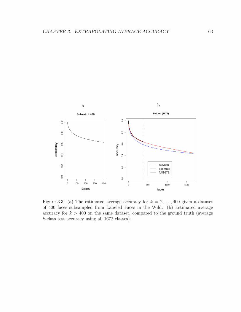
CHAPTER 3. EXTRAPOLATING AVERAGE ACCURACY 63
a b
0 100 200 300 400
0.0
0.2
0.4
0.6
0.8
1.0
Subset of 400
faces
accu
racy
0 500 1000 1500
0.0
0.2
0.4
0.6
0.8
1.0
Full set (1672)
faces
accu
racy
sub400estimatefull1672
Figure 3.3: (a) The estimated average accuracy for k = 2, . . . , 400 given a datasetof 400 faces subsampled from Labeled Faces in the Wild. (b) Estimated averageaccuracy for k > 400 on the same dataset, compared to the ground truth (averagek-class test accuracy using all 1672 classes).

CHAPTER 3. EXTRAPOLATING AVERAGE ACCURACY 64
for ` = 1, . . . ,m. Here we take m = 10000. We model the function D(u) as a
non-negative linear combination of basis functions,
D(u) =m∑`=1
β`h`(u),
with β` ≥ 0. The non-negativity constraint on the coefficients β, combined with the
linear spline basis, ensures that D(u) is a monotonic and convex function on [0, 1].
We have found that in many simulated examples, D(u) appears to be monotone
and convex, and we have also found that including the monotonicity and convexity
constraint in the estimation procedure improves performance in practical examples.
The resulting estimated generalization accuracies, computed using (3.1), are plotted
in Figure (3.3) (b). As we already mentioned, to assess the quality of the estimated
average accuracy, we compare them to the ‘ground truth’ accuracy curve obtained by
using all 1672 examples to compute the the average test risk.
To get an idea of the accuracy and variance of the accuracy curve estimates for
varying sample sizesK, we repeat this procedure multiple times forK ∈ {100, 200, 400, 800}.The results, again compared to the ground truth computed from the full data set, are
illustrated in figure 3.4.
3.4.2 Telugu OCR example
While the previous example was a perfect fit to the assumptions of the framework, we
also want to see how well the method works when some of the assumptions may be
violated. Towards this end we apply performance extrapolation in an optical character
recognition example (Achanta and Hastie 2015) for predicting the accuracy on 400
classes of Telugu characters from a subsample of size K = 20. We consider the use of
five different classifiers: Naive Bayes, logistic regression, SVM, ε-nearest neighbors2,
and a deep convolutional neural network3. Of the five classifiers, only Naive Bayes
satisfies the marginal classifier assumption. Again, we compare the result of our
model to the ground truth obtained by using the full dataset.
2m-nearest neighbors with m = εn for fixed ε > 03The network architecture is as follows: 48x48-4C3-MP2-6C3-8C3-MP2-32C3-50C3-MP2-200C3-SM.
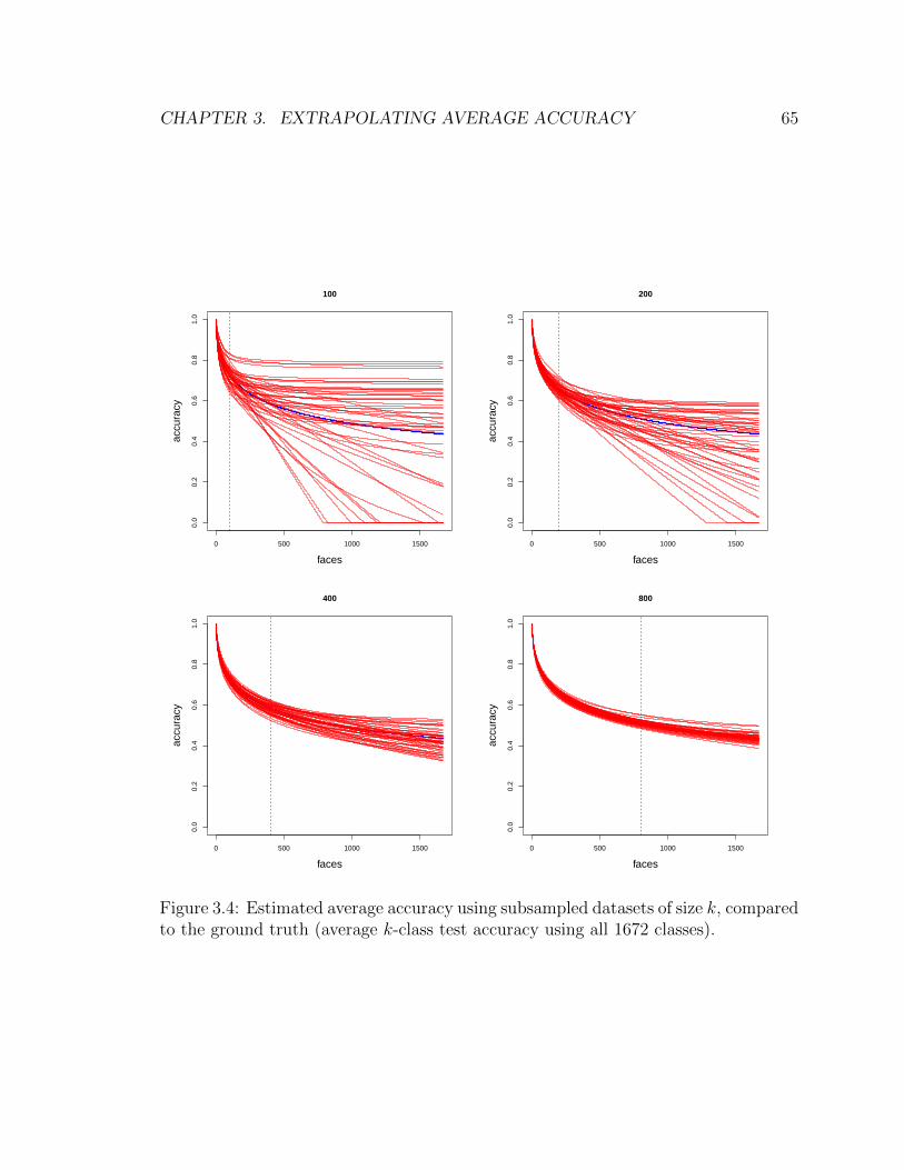
CHAPTER 3. EXTRAPOLATING AVERAGE ACCURACY 65
0 500 1000 1500
0.0
0.2
0.4
0.6
0.8
1.0
100
faces
accu
racy
0 500 1000 1500
0.0
0.2
0.4
0.6
0.8
1.0
200
faces
accu
racy
0 500 1000 1500
0.0
0.2
0.4
0.6
0.8
1.0
400
faces
accu
racy
0 500 1000 1500
0.0
0.2
0.4
0.6
0.8
1.0
800
faces
accu
racy
Figure 3.4: Estimated average accuracy using subsampled datasets of size k, comparedto the ground truth (average k-class test accuracy using all 1672 classes).

CHAPTER 3. EXTRAPOLATING AVERAGE ACCURACY 66
Classifier Test acc(20) Test acc(400) ˆAGA400
Naive Bayes 0.951 0.601 0.858Logistic 0.922 0.711 0.812
SVM 0.860 0.545 0.687ε-NN 0.951 0.591 0.410
Deep neural net 0.995 0.986 0.907
Table 3.1: Performance extrapolation: predicting the accuracy on 400 classes usingdata from 20 classes on a Telugu character dataset. ε = 0.002 for ε-nearest neighbors.
The results are displayed in Table 3.1. To our surprise, the worst absolute differ-
ence between ground truth and estimated average accuracy was in the case of Naive
Bayes (|δ| = 0.257) which satisfies the marginal property. All other classifiers had
absolute errors less than 0.2. It is also interesting to note that, even though Naive
Bayes and ε-nearest neighbors have the same test accuracy on the subset, that the
predicted accuracy on 400 differs greatly between then (0.858 vs 0.400).
While further work is still needed to better understand the performance of the pro-
posed performance extrapolation method, both for marginal classifiers (which satisfy
the theoretical assumptions) and non-marginal classifiers (which do not), the results
obtained in these two examples are encouraging in the sense that useful predictions
were obtained both for marginal and non-marginal classifiers.

Chapter 4
Inference of mutual information
4.1 Motivation
As we discussed in the introduction, the mutual information I(X;Y ) provides one
method for the supervised evaluation of representations. Recall that Shannon’s mu-
tual information I(X;Y ) is fundamentally a measure of dependence between random
variables X and Y , defined as
I(X;Y ) =
∫p(x, y) log
p(x, y)
p(x)p(y)dxdy.
Various properties of I(~g(~Z);Y ), such as sensitivity to nonlinear relationships, sym-
metry, and invariance to bijective transformations, make it ideal for quantifying the
information between a representation of an input vector ~g(~Z) and a (possibly vector-
valued) response Y .
However, current methods estimating mutual information for high-dimensional
data either require large and over-parameterized generative models, or work only
for discrete responses. For continuous (X, Y ), one can tractably estimate mutual
information by assuming a multivariate Gaussian model: however, this approach
essentially assumes a linear relationship between the input and output, and hence
fails to quantify nonlinear dependencies. Meanwhile, in the case of a discrete response
Y , one can obtain a lower bound on the mutual information by using the confusion
67

CHAPTER 4. INFERENCE OF MUTUAL INFORMATION 68
matrix of a classifier. This is the most popular approach for estimating mutual
information in neuroimaging studies, but suffers from known shortcomings (Gastpar,
Gill, and Theunissen 2009, Quian Quiroga and Panzeri 2009). The idea of linking
classification performance to mutual information dates back to the beginnings of
information theory: Shannon’s original motivation was to characterize the minimum
achievable error probability of a noisy communication channel. More explicitly, Fano’s
inequality (Fano 1961) provides a lower bound on mutual information in relation to
the optimal prediction error, or Bayes error. Fano’s inequality can be further refined
to obtain a tighter lower bound on mutual information (Tebbe and Dwyer 1968.)
However, a shortcoming to all of these classification-based approaches is that if Y is
not already discrete, the discretization of the response Y necessarily loses information.
In this chapter, we develop an analogue of Fano’s inequality for the identification
task, rather than the classification task, which can therefore be applied to the case
of a continuous response Y . In this way, we derive a new machine-learning based
estimator of mutual information I(X;Y ) which can be applied without the need to
discretize a continuous response.
As we saw in Chapter 2, the identification task is highly related to the randomized
classification framework. Therefore, we analyse the identification risk by means of
the k-class average Bayes accuracy, which provides an upper bound to identification
accuracy. Our main theoretical contributions are (i) the derivation of a tight lower
bound on mutual information as a function of k-class average Bayes accuracy, and
(ii) the derivation of an asymptotic relationship between the k-class average Bayes
accuracy and the mutual information. Our method therefore estimates the k-class
Bayes identification accuracy to be translated into estimate of the mutual information.
Our method complements the collection of existing approaches for estimating
mutual information in the sense that it allows the leveraging of different kinds of prior
assumptions than ones previously considered in the literature. Our target application
is when the relationship between the random variables (X, Y ) is well-described by
a parametric regression model E[Y |X = x] = fθ(x). An important special case is
when a sparse relationship exists between the predictor and response. As we will
demonstrate, exploiting sparsity assumptions can vastly improve the efficiency of

CHAPTER 4. INFERENCE OF MUTUAL INFORMATION 69
estimation in high-dimensional settings.
The rest of the chapter is organized as follows. Section 4.2 establishes the theoret-
ical results linking average Bayes accuracy and mutual information, and Section 4.3
describes our proposed identification-based estimator of mutual information based on
the theory. We present one simulation example in section 4.4, but will we also see
some real data applications in the next chapter.
4.2 Average Bayes accuracy and Mutual informa-
tion
4.2.1 Problem formulation and result
Let P denote the collection of all joint densities p(x, y) on finite-dimensional Euclidean
space. For ι ∈ [0,∞) define Ck(ι) to be the largest k-class average Bayes error attained
by any distribution p(x, y) with mutual information not exceeding ι:
Ck(ι) = supp∈P:I[p(x,y)]≤ι
ABAk[p(x, y)].
A priori, Ck(ι) exists since ABAk is bounded between 0 and 1. Furthermore, Ck is
nondecreasing since the domain of the supremum is monotonically increasing with ι.
It follows that for any density p(x, y), we have
ABAk[p(x, y)] ≤ Ck(I[p(x, y)]).
Hence Ck provides an upper bound for average Bayes error in terms of mutual infor-
mation.
Conversely we have
I[p(x, y)] ≥ C−1k (ABAk[p(x, y)])
so that C−1k provides a lower bound for mutual information in terms of average Bayes

CHAPTER 4. INFERENCE OF MUTUAL INFORMATION 70
error.
On the other hand, there is no nontrivial lower bound for average Bayes error in
terms of mutual information, nor upper bound for mutual information in terms of
average Bayes error, since
infp∈P:I[p(x,y)]≤ι
ABAk[p(x, y)] =1
k.
regardless of ι.
In the following sections we determine the value of Ck(ι), leading to the following
result.
Theorem 4.2.1 For any ι > 0, there exists cι ≥ 0 such that defining
Qc(t) =exp[ctk−1]∫ 1
0exp[ctk−1]
,
we have ∫ 1
0
Qcι(t) logQcι(t)dt = ι.
Then,
Ck(ι) =
∫ 1
0
Qcι(t)tk−1dt.
We obtain this result by first reducing the problem to the case of densities with
uniform marginals, then doing the optimization over the reduced space.
4.2.2 Reduction
Let p(x, y) be a density supported on X × Y , where X is a subset of Rd1 with a
non-empty interior, and Y is a subset of Rd2 , also with non-empty interior, and such
that p(x) is uniform on X and p(y) is uniform on Y .
Now let Punif denote the set of such distributions: in other words, Punif is the
space of joint densities in Euclidean space with uniform marginals over the marginal

CHAPTER 4. INFERENCE OF MUTUAL INFORMATION 71
supports. In this section, we prove that
Ck(ι) = supp∈P:I[p(x,y)]≤ι
ABAk[p(x, y)] = supp∈Punif :I[p(x,y)]≤ι
ABAk[p(x, y)],
thus reducing the problem of optimizing over the space of all densities to the problem
of optimizing over densities with uniform marginals.
Also define Pbounded to be the space of all densities p(x, y) with finite-volume
support. Since uniform distributions can only be defined over sets of finite volume,
we have
Punif ⊂ Pbounded ⊂ P .
Therefore, it is necessary to first show that
supp∈P:I[p(x,y)]≤ι
ABAk[p(x, y)] = supp∈Pbounded:I[p(x,y)]≤ι
ABAk[p(x, y)].
This is accomplished via the following lemma.
Lemma 4.2.1 (Truncation). Let p(x, y) be a density on Rdx × Rdy with I[p(x, y)] <
∞. For all ε > 0, there exists a subset X ⊂ Rdx with finite volume with respect
to dx-dimensional Lesbegue measure, and a subset Y ⊂ Rdy with finite volume with
respect to dy-dimensional Lesbegue measure, such that defining
p(x, y) =I{(x, y) ∈ X × Y}∫X×Y p(x, y)dxdy
p(x, y),
we have
|I[p]− I[p]| < ε
and
|ABAk[p]− ABAk[p]| < ε.
Proof. Recall the definition of the Shannon entropy H:
H[p(x)] = −∫p(x) log p(x)dx.

CHAPTER 4. INFERENCE OF MUTUAL INFORMATION 72
It is a well-known in information theory that
I[p(x, y)] = H[p(x)] + H[p(y)]− H[p(x, y)].
There exists a sequence (Xi,Yi)∞i=1 where (Xi)∞i=1 is an increasing sequence of finite-
volume subsets of Rdx and (Yi)∞i=1 is an increasing sequence of finite-volume subsets
of Rdy , and limi→∞Xi = Rdx , limi→∞ Yj. Define
pi(x, y) =I{(x, y) ∈ Xi × Yi}∫Xi×Yi p(x, y)dxdy
p(x, y)
Note that pi gives the conditional distribution of (X, Y ) conditional on (X, Y ) ∈Xi × Yi. Furthermore, it is convenient to define p∞ = p. We can find some i1, such
that for all i ≥ i1, we have ∣∣∣∣∫x/∈Xi
p(x) log p(x)dx
∣∣∣∣ < ε
6∣∣∣∣∫y/∈Yi
p(y) log p(y)dy
∣∣∣∣ < ε
6∣∣∣∣∫(x,y)/∈Xi×Yi
p(x, y) log p(x, y)dxdy
∣∣∣∣ < ε
6
and also such that
− log
[∫x,y∈Xi×Yi
p(x, y)dxdy
]<ε
2
Then, it follows that
|I[p]− I[pi]| < ε
for all i ≥ i1.
Now we turn to the analysis of average Bayes error. Let fi denote the Bayes
k-class classifier for pi(x, y) and f∞ the Bayes k-class classifier for p(x, y): recall that
by definition,
ABAk[pi] = Prpi
[fi(Y(1), ..., Y (k), X) = Y (1)]

CHAPTER 4. INFERENCE OF MUTUAL INFORMATION 73
where the probability is taken with respect to the joint distribution of Y (1), . . . , Y (k)
drawn from p(y), and X drawn from the conditional distribution p(x|Y (1)). Define
εi = Prp
[(Y (1), ..., Y (k), X) /∈ Yki ×Xi];
by continuity of probability we have limi εi → 0. We claim that
|ABAk[pi]− ABAk[p]| ≤ εi.
Given the claim, the proof is completed by finding i > i1 such that εi < ε, and defining
X = Xi, Y = Yi.Consider using fi to obtain a classification rule for p(x, y): define
fi =
fi(y(1), . . . , y(k), x) when (y(1), . . . , y(k), x) ∈ X ki × Yi
0 otherwise.
We have
ABAk[p] = supf
Prp
[f(Y (1), . . . , Y (k), X) = Y (1)]
≥Prp
[fi(Y(1), . . . , Y (k), X) = Y (1)]
=(1− εi) Prp
[fi(Y(1), . . . , Y (k), X) = Y (1)|(Y (1), . . . , Y (k), X) ∈ X k
i × Yi]
+ εi Prp
[fi(Y(1), . . . , Y (k), X) = Y (1)|(Y (1), . . . , Y (k), X) /∈ X k
i × Yi]
=(1− εi) Prp
[fi(Y(1), . . . , Y (k), X) = Y (1)] + εi0
=(1− εi)ABAk[pi] ≥ ABAk[pi]− εi.
In other words, when pi is close to p, the Bayes classification rule for pi obtains close
to the Bayes rate when the data is generated under p.
Now consider the reverse scenario of using fp to perform classification under pi.
This is equivalent to generating data under p(x, y), performing classification using
f , then only evaluating classification accuracy conditional on (Y (1), ..., Y (k), X) ∈

CHAPTER 4. INFERENCE OF MUTUAL INFORMATION 74
Yki ×Xi. Therefore,
ABAk[pi] = supf
Prpi
[f(Y (1), . . . , Y (k), X) = Y (1)]
≥Prpi
[fi(Y(1), . . . , Y (k), X) = Y (1)]
= Prp
[fi(Y(1), . . . , Y (k), X) = Y (1)|(Y (1), . . . , Y (k), X) ∈ Yki ×Xi]
=1
1− εiPrp
[I{(X(1), ..., X(k), Y ) ∈ Yki ×Xi} and fi(Y(1), . . . , Y (k), X) = Y (1)]
≥ 1
1− εi
(1− Pr
p[I{(Y (1), ..., Y (k), X) /∈ Yki ×Xi}]− Pr
p[fp(Y
(1), . . . , Y (k), X) 6= Y (1)]]
)=
ABAk[p]− εi1− εi
≥ ABAk[p]− εi.
In other words, when pi is close to p, the Bayes classification rule for p obtains close
to the Bayes rate when the data is generated under pi.
Combining the two directions gives |ABAk[pi]− ABAk[p]| ≤ εi, as claimed. �
One can go from bounded-volume sets to uniform distributions by adding auxillary
variables. To illustrate the intution, consider a density p(x) on a set of bounded
volume, X . Introduce a variable W such that conditional on X = x, we have W
uniform on [0, p(x)]. It follows that the joint density p(x,w) = 1 and is supported on
a set X ′ = X × [0,∞]. Furthermore, X ′ is of bounded volume (in fact, of volume 1)
since ∫X ′dxdw =
∫X ′p(x,w)dxdw = 1.
Therefore, to accomplish the reduction from P to Punif , we start with a density
p(x, y) ∈ P , and using Lemma 4.2.1, find a suitable finite-volume truncation p(x, y).
Finally, we introduce auxillary variables w and z so that the expanded joint distribu-
tion p(x,w, y, z) has uniform marginals p(x,w) and p(y, z). However, we still need to
check that the introduction of auxillary variables preserves the mutual information
and average Bayes error; this is the content of the next lemma.
Lemma 4.2.2 Suppose X, Y , W , Z are continuous random variables, and that W ⊥

CHAPTER 4. INFERENCE OF MUTUAL INFORMATION 75
Y |Z, Z ⊥ X|Y , and W ⊥ Z|(X, Y ). Then,
I[p(x, y)] = I[p((x,w), (y, z))],
and also for all k ∈ {2, 3, . . . , },
ABAk[p(x, y)] = ABAk[p((x,w), (y, z))].
Proof. Due to conditional independence relationships, we have
p((x,w), (y, z)) = p(x, y)p(w|x)p(z|y).
It follows that
I[p((x,w), (y, z))] =
∫dxdwdydz p(x, y)p(w|x)p(z|w) log
p((x,w), (y, z))
p(x,w)p(y, z)
=
∫dxdwdydz p(x, y)p(w|x)p(z|w) log
p(x, y)p(w|x)p(z|y)
p(x)p(y)p(w|x)p(z|y)
=
∫dxdwdydz p(x, y)p(w|x)p(z|w) log
p(x, y)
p(x)p(y)
=
∫dxdy p(x, y) log
p(x, y)
p(x)p(y)= I[p(x, y)].
Also,
ABAk[p((x,w), (y, z))] =
∫ [ k∏i=1
p(xi, wi)dxidwi
]∫dydz max
ip(y, z|xi, wi).
=
∫ [ k∏i=1
p(xi, wi)dxidwi
]∫dy max
ip(y|xi)
∫dz p(z|y).
=
∫ [ k∏i=1
p(xi)dxi
][k∏i=1
∫dwip(wi|xi)
]∫dy max
ip(y|xi)
= ABAk[p(x, y)].
�

CHAPTER 4. INFERENCE OF MUTUAL INFORMATION 76
Combining these lemmas gives the needed reduction, given by the following the-
orem.
Theorem 4.2.2 (Reduction.)
supp∈P:I[p(x,y)]≤ι
ABAk[p(x, y)] = supp∈Punif :I[p(x,y)]≤ι
ABAk[p(x, y)].
The proof is trivial given the previous two lemmas.
4.2.3 Proof of theorem
Proof of theorem 4.2.1
Using Theorem 4.2.2, we have
Ck(ι) = supp∈Punif :I[p(x,y)]≤ι
ABAk[p(x, y)].
Define σ(ι) =∫ 1
0Qcι(t)t
k−1dt: our goal is to establish that Ck(ι) = σ(ι). Note
that σ(ι) is the same function which appears in Lemma B.1.5 and the same bound as
established in Lemma B.1.4.
Define the density pι(x, y) where
pι(x, y) =
gι(y − x) for x ≥ y
gι(1 + y − x) for x < y
where
gι(x) =d
dxGι(x)
and Gι is the inverse of Qc.
One can verify that I[pι] = ι, and
ABAk[p] =
∫ 1
0
Qcι(t)tk−1dt.

CHAPTER 4. INFERENCE OF MUTUAL INFORMATION 77
This establishes that
Ck(ι) ≥∫ 1
0
Qcι(t)tk−1dt.
It remains to show that for all p ∈ Punif with I[p] ≤ ι, that ABAk[p] ≤ ABAk[pι].
Take p ∈ Punif such that I[p] ≤ ι. Letting Y (1), ..., Y (k) ∼ Unif[0, 1], and X ∼Unif[0, 1] define Zi(x) = p(x|Yi). We have E(Z1(x)) and,
I[p(x, y)] = E(Z1(X) logZ1(X))
while
ABAk[p(x, y)] = k−1E(maxiZi(X)).
Letting Gx be the distribution of Z(x), we have
E[Gx] = 1
I[p(x, y)] = E(I[GX ])
ABAk[p(x, y)] = E(ψk[GX ])
where the expectation is taken over X ∼ Unif[0, 1] and where E[G], I[G], and ψk[G]
are defined as in Lemma B.1.4.
Define the random variable J = I[GY ]. We have
ABAk[p(x, y)] = E(ψk[GX ])
=
∫ 1
0
ψk[GX ]dy
≤∫ 1
0
(sup
G:I[G]≤I[Gx]
ψk[G]
)dy
=
∫ 1
0
σ(I[Gx])dy = E[σ(J)].
Now, since f is concave by Lemma B.1.5, we can apply Jensen’s inequality to conclude
that
ABAk[p(x, y)] = E[σ(J)] ≤ σ(E[J ]) = σ(ι),

CHAPTER 4. INFERENCE OF MUTUAL INFORMATION 78
which completes the proof. �
4.3 Estimation
Now let us return to the problem of estimating the mutual information I(X;Y ) based
on observations (xi, yi)ni=1 drawn iid from the joint distribution.
We would like to use the cross-validated identication accuracy (1.1) as a basis for
estimating the mutual information. How this works is as follows.
Define the k-class average identification accuracy as the expected value of the
cross-validated identification accuracy (1.1),
AIAkdef= E[TAk,CV ].
As we argued in section 2.4.7, the k-class average identification accuracy is a lower
bound for the k-class average Bayes accuracy,
AIAk ≤ ABAk.
Finally, applying the theorem 4.2.1, we have
I(X;Y ) ≥ C−1k (ABAk) ≥ C−1
k (AIAk).
Replacing AIAk with its estimate, TAk,CV , yields the estimator
IIdent(X;Y )def= C−1
k (TAk,CV ) (4.1)
Since we use a lower bounding theorem to obtain the estimate, the estimated
mutual information tends to be an underestimate of the true result. Therefore, we get
a better estimate if we choose a regression model which maximizes the identification
accuracy. For example, when it is known that a sparse linear relationship is a good
fit for the regression function E[Y |X = x], then it would be advised to use sparse
linear regression models, such as elastic net (Zou and Hastie 2005), to obtain the

CHAPTER 4. INFERENCE OF MUTUAL INFORMATION 79
identification accuracy.
4.4 Simulation
In order to demonstrate the advantages of our identification-based estimator of mutual
information, we ran a simple simulation study under relatively ideal conditions. Our
simulation model was a sparse multivariate linear model of the form
(Y1, Y2) = (X1, X2)TB + ε
where B is a randomly generated coefficient matrix. Then we added extra noise di-
mensions X3, X4, . . . , Xp for p ranging up to 600. For data with sample size n = 1000,
we compared the estimates of mutual information I(X;Y ) obtained using the nearest-
neighbor estimator (Mnatsakanov et al. 2008, implemented in FNN) with our method,
using both ordinary least-squares and LASSO regression (using cross-validation to
choose λ, as implemented in Friedman, Hastie, and Tibshirani 2010).
The results of the simulation are displayed in Figure 4.1. We see that for small
p, the nearest-neighbor method and our method, for both OLS and LASSO perform
similarly. As p increases to 10, the nearest neighbor estimator rapidly deteriorates,
while OLS and LASSO-based estimators remain at similar levels. For p larger than
100, the LASSO-based estimator begins to outperform the OLS-based estimator, as
LASSO better leverages the sparsity of the data. We see that the LASSO-based esti-
mator is highly robust to addition of noise predictors up to the largest dimensionality
we attempted in the simulation, p = 600.
We will see additional examples in the next chapter, including a simulation exam-
ple involving a dense model.

CHAPTER 4. INFERENCE OF MUTUAL INFORMATION 80
Figure 4.1: Estimation of mutual information in simulated example. Comparisonof IIdent using k = {10, 20} and using OLS or LASSO for regression of Y on X, tononparametric nearest-neighbors estimator (Mnatsakanov et al. 2008). The dimen-sionality of X is varied by adding noise predictors, up to p = 600. Top plot: p = 2(no noise predictors) to p = 10. Bottom plot: p = 100 to p = 600.

Chapter 5
High-dimensional inference of
mutual information
5.1 Motivation
In the previous chapter, we saw that the identification accuracy of predicting Y given
X can be used to yield a lower bound on I(X;Y ). This relied on the inequality
relating k-class average Bayes accuracy and mutual information. However, because
in some cases the mutual information may be much higher than the lower bound,
the estimator IIdent (4.1) may remain an underestimate of mutual information, even
under favorable sample size conditions. In other words, the estimator IIdent is not
consistent. On the other hand, the theory behind IIdent relies on extremely weak
assumptions. This makes the estimator quite generally applicable, but on the other
hand, much better estimators may be available in certain applications where much
stronger assumptions can be made.
In this chapter we develop yet another estimator of mutual information based on
identification accuracy, but this time making relatively strong assumptions relating to
the dimensionality of the data and the dependence structure of the components. As we
will spell out in more detail in section 5.2.1, we assume a setting where both (X, Y )
are high-dimensional, and where the true mutual information I(X;Y ) is relatively
low. Furthermore, we require the components of X to have “low dependence,” in a
81

CHAPTER 5. HIGH-DIMENSIONAL INFERENCEOFMUTUAL INFORMATION82
certain sense.
We expect that these assumptions are well-matched to applications such as fMRI
data, where the effective dimensionality of the data is large, but where the noise level
limits the mutual information between X and Y .
The estimator of mutual information we develop in this chapter is based on ex-
ploiting a universality property that arises in high-dimensions. This universality
phenomenon allows us to establish a relationship between the mutual information
I(X;Y ) and the k-class average Bayes accuracy, ABAk. In short, we will identify a
function πk (which depends on k),
ABAk ≈ πk(√
2I(X;Y )) (5.1)
and that this approximation becomes accurate under a limit where I(X;Y ) is small
relative to the dimensionality of X, and under the condition that the components of
X are approximately independent. The function πk is given by
πk(c) =
∫Rφ(z − c)Φ(z)k−1dz.
This formula is not new to the information theory literature: it appears in the error
rate of an orthogonal constellation (Cioffi 2014). What is surprising is that the same
formula can be used to approximate the error rate in much more general class of
classification problems1–this is precisely the universality result which provides the
basis for our proposed estimator.
Figure 5.1 displays the plot of πk for several values of k. For all values of k, πk(µ)
is monotonically increasing in µ, and tends to 1 as µ→∞, which is what we expect
since if I(X;Y ) is large, then we should be able to achieve perfect accuracy. Another
intuitive fact is that πk(0) = 1k, since after all, an uninformative response cannot lead
to above-chance classification accuracy.
1An intuitive explanation for this fact is that points from any high-dimensional distribution liein an orthogonal configuration with high probability.

CHAPTER 5. HIGH-DIMENSIONAL INFERENCEOFMUTUAL INFORMATION83
Figure 5.1: Left: The function πk(µ) for k = {2, 10}.
The estimator we propose is
IHD =1
2(π−1
k (TAk,CV ))2, (5.2)
obtained by inverting the relation (5.1), then substituting an estimate of the identi-
fication accuracy TAk,CV for ABAk.
5.2 Theory
5.2.1 Assumptions
Our asymptotic theory applies to an infinite sequence of densities p[d](x, y) for d =
1, 2, . . ., where the following conditions hold.
A1. The mutual information converges to a finite constant: limd→∞ I[p[d](x, y)] =
ι <∞.
For all integers k > 2, we also require the following assumptions A2-A4 to hold. For
d = 1, . . ., let (X(i), Y (i)) be drawn i.i.d. from p[d](x, y), for i = 1, . . . , k. Define
`ij = log p[d](X(i)|Y (i))
Then:

CHAPTER 5. HIGH-DIMENSIONAL INFERENCEOFMUTUAL INFORMATION84
A2. There exists a sequence of scaling constants a[d]ij and b
[d]ij such that the random
vector (aij`[d]ij + b
[d]ij )i,j=1,...,k converges in distribution to a multivariate normal
distribution.
A3. Define
u[d](x, y) = log p[d](x, y)− log p[d](x)− log p[d](y).
There exists a sequence of scaling constants a[d], b[d] such that
a[d]u[d](X(1), Y (2)) + b[d]
converges in distribution to a univariate normal distribution.
A4. For all i 6= k,
limd→∞
Cov[u[d](X(i), Y (j)), u[d](X(k), Y (j))] = 0.
Assumptions A1-A4 are satisfied in a variety of natural models. One example is
a multivariate Gaussian sequence model where X ∼ N(0,Σd) and Y = X + E with
E ∼ N(0,Σe), where Σd and Σe are d × d covariance matrices, and where X and E
are independent. Then, if dΣd and Σe have limiting spectra H and G respectively, the
joint densities p(x, y) for d = 1, . . . , satisfy assumptions A1 - A4. Another example
is the multivariate logistic model, which we describe in section 5.3.1.
5.2.2 Limiting universality
We obtain the universality result in two steps. First, we link the average Bayes error
to the moments of some statistics Zi. Secondly, we use Taylor approximation in order
to express I(X;Y ) in terms of the moments of Zi. Connecting these two pieces yields
the formula (5.1).
Let us start by rewriting the average Bayes error:
ABAk = Pr[p(X|Y (1)) >k
maxj=2
p(X|Y (j))].

CHAPTER 5. HIGH-DIMENSIONAL INFERENCEOFMUTUAL INFORMATION85
where the expectation is taken over the joint distribution Y (1), . . . , Y (k) i.i.d.∼ p(y) and
X ∼ p(x|Y (1)). Defining the statistic Zi = log p(X|Y (i)) − log p(X|Y (1)), we obtain
ABAk = Pr[maxkj=2 Zj < 0]. The key assumption we need is that Z2, . . . , Zk are
asymptotically multivariate normal. If so, the following lemma allows us to obtain a
formula for the average Bayes accuracy.
Lemma 1. Suppose (ζ1, ζ2, . . . , ζ`) are jointly multivariate normal, with E[ζi] =
−α Var(ζi) = β ≥ 0, Cov(ζi, ζj) = γ for i = 1, . . . , ` and j = 1, . . . , ` with i 6= j.
Then, letting
µ =E[−ζ1]√
12Var(ζ1 − ζ2)
=α√β − γ
,
ν2 =Cov(ζ1, ζ2)
12Var(ζ1 − ζ2)
=γ
β − γ,
we have
Pr[0 >k
maxi=1
ζi] = Pr[W > Mk−1]
=
∫1√
2πν2e−
(w−µ)2
2ν2 Φ(w)k−1dw,
where W ∼ N(µ, ν2) and Mk−1 is the maximum of k−1 independent standard normal
variates, which are independent of W .
Remark. To see why the assumption that Z2, . . . , Zk are multivariate normal
might be justified, suppose that X and Y have the same dimensionality d, and that
joint density factorizes as
p[d](x, y) =d∏i=1
pi(xi, yi)
where x(j)i , yi are the ith scalar components of the vectors x and y. Further assume
that∞
supi=1
E[pi(Xi, Yi)2] <∞.
Then,
Zi =d∑
m=1
log pm(xm|y(i)m )− log pm(xm|y(1)
m ).

CHAPTER 5. HIGH-DIMENSIONAL INFERENCEOFMUTUAL INFORMATION86
The d terms log pm(xm|y(i)m )−log pm(xm|y(1)
m ) are independent across the indicesm, but
dependent between the i = 2, . . . , k. Therefore, the multivariate central limit theorem
can be applied to conclude that the vector (Z2, . . . , Zk) can be scaled to converge to a
multivariate normal distribution. While the componentwise independence condition is
not a realistic assumption, the key property of multivariate normality of (Z2, . . . , Zk)
holds under more general conditions, and appears reasonable in practice.
Proof. We can construct independent normal variates G0, G1, . . . , Gk such that
G0 ∼ N(0, γ)
and
Gi ∼ N(0, β − γ) for i = 1, . . . , `
such that
ζi = −α +G0 +Gi for i = 1, . . . , `
Hence
Pr[0 >k
maxi=1
ζi] = Pr[k
mini=1
G0 +Gi − α > 0]
= Pr[k
mini=1
Gi > α−G0]
= Pr[k
mini=1
Gi√β − γ
>α−G0√β − γ
].
Since Gi√β−γ are iid standard normal variates, and since −α−G0√
β−γ ∼ N(µ, ν2) for µ and
ν2 given in the statement of the Lemma, the proof is completed via a straightforward
computation. �
It remains to link the moments of Zi to I(X;Y ). This is accomplished by approx-
imating the logarithmic term by the Taylor expansion
logp(x, y)
p(x)p(y)≈ p(x, y)− p(x)p(y)
p(x)p(y)−(p(x, y)− p(x)p(y)
p(x)p(y)
)2
+ . . . .
The is the intuition behind the theorem which establishes (5.1), which we now state.

CHAPTER 5. HIGH-DIMENSIONAL INFERENCEOFMUTUAL INFORMATION87
Theorem 1. Let p[d](x, y) be a sequence of joint densities for d = 1, 2, . . .. Further
assume conditions A1 - A4. Then for ABAk as defined above, we have
limd→∞
ABAk = πk(√
2ι)
where
πk(c) =
∫Rφ(z − c)Φ(z)k−1dz
where φ and Φ are the standard normal density function and cumulative distribution
function, respectively.
Proof.
For i = 2, . . . , k, define
Z[d]i = log p[d](X|Y (i))− log p[d](X|Y (1)).
Then, we claim that as d→∞, ~Z [d] = (Z[d]2 , . . . , Z
[d]k ) converges in distribution to
~Z [d] ∼ N
−2ι,
4ι 2ι · · · 2ι
2ι 4ι · · · 2ι...
.... . .
...
2ι 2ι · · · 4ι
.
Combining the claim with Lemma 1 yields the desired result.
To prove the claim, it suffices to derive the limiting moments
limd→∞
E[Z[d]i ] = −2ι,
limd→∞
Var[Z[d]i ] = 4ι,
limd→∞
Cov[Z[d]i , Z
[d]j ] = 2ι,
for i 6= j, since then assumption A2 implies the existence of a multivariate normal
limiting distribution with the given moments.
Before deriving the limiting moments, note the following identities. Let Y = Y (1)

CHAPTER 5. HIGH-DIMENSIONAL INFERENCEOFMUTUAL INFORMATION88
and Y ′ = Y (2). Then for all d ≥ 1,
E[eu[d](X,Y ′)] =
∫p[d](x)p[d](y)eu
[d](x,y)dxdy =
∫p[d](x, y)dxdy = 1.
Therefore, from assumption A3 and the formula for gaussian exponential moments,
we have
limd→∞
E[u[d](X, Y ′)]− 1
2Var[u[d](X, Y ′)] = 0.
In other words, u[d](X, Y ′) converges in distribution to N(−σ2
2, σ2), where we define
σ2 = limd→∞
Var[u[d](X, Y ′)].
Meanwhile, by applying assumption A2,
ι = limd→∞
I[p[d](x, y)] = limd→∞
∫p[d](x, y)u[d](x, y)dxdy = lim
d→∞
∫p[d](x)p[d](y)eu
[d](x,y)u[d](x, y)dxdy
= limd→∞
E[eu[d](X,Y ′)u[d](X, Y ′)]
Now note that for Z ∼ N(µ, σ2), we have E[ZeZ ] = (µ + σ2)eµ+σ2
2 . Since
u[d](X, Y ′) converges in distribution to N(−σ2
2, σ2), we get
ι = limd→∞
E[eu[d](X,Y ′)u[d](X, Y ′)] =
1
2σ2.
Therefore,
σ2 = 2ι,
and it follows that
limd→∞
E[u[d](X ′, Y )] = −ι.
Meanwhile, since I[p[d](X, Y )] = E[u[d](X, Y )], we have
limd→∞
E[u[d](X, Y )] = ι.

CHAPTER 5. HIGH-DIMENSIONAL INFERENCEOFMUTUAL INFORMATION89
Once again by applying A2, we get
limd→∞
Var[u[d](X, Y )] = limd→∞
∫(u[d](x, y)− ι)2p[d](x, y)dxdy
= limd→∞
∫(u[d](x, y)− ι)2eu
[d](x,y)p[d](x)p[d](y)dxdy
= limd→∞
E[(u[d](X, Y ′)− ι)2eu[d](X,Y ′)]
=
∫(z − ι)2ez
1√4πι
e−(z+ι)2
4ι dz (applying A2)
=
∫(z − ι)2 1√
4πιe−
(z−ι)24ι dz
= 2ι.
We now proceed to derive the limiting moments. We have
limd→∞
E[Z[d]i ] = lim
d→∞E[log p[d](X|Y ′)− log p[d](X|Y )]
= limd→∞
E[u[d](X, Y ′)− u[d](X, Y )] = −2ι.
Also,
limd→∞
Var[Z [d]] = limd→∞
Var[u[d](X, Y ′)− u[d](X, Y )]
= limd→∞
Var[u[d](X, Y ′)] + Var[u[d](X, Y )] (using assumption A4)
= 4ι,
and similarly
limd→∞
Cov[Z[d]i , Z
[d]j ] = lim
d→∞Var[u[d](X, Y )] (using assumption A4)
= 2ι.
This concludes the proof. �.

CHAPTER 5. HIGH-DIMENSIONAL INFERENCEOFMUTUAL INFORMATION90
5.3 Examples
We demonstrate the application of our proposed estimators, IIdent, which was in-
troduced in the previous chapter, and the estimator IHD based on high-dimensional
asymptotics, as defined in (5.2).
We compare our methods to a number of existing methods for mutual information.
For any k-class classification task, define the k×k confusion matrix M as the matrix
whose i, j counts how many times a output in the ith class was classified to the jth
class.
The estimator IFano is based on Fano’s inequality, which reads
H(Z|Y ) ≤ H(1− BA) + (1− BA) log ||Z| − 1|
where BA is Bayes accuracy, and H(e) is the entropy of a Bernoulli random variable
with probability e. Replacing H(Z|Y ) with H(X|Y ) and replacing BA with the test
accuracy TA, we get the estimator
IFano = log(K)− (1− TA) log(K − 1) + (1− TA) log(1− TA) + TA log(TA).
Meanwhile, the confusion matrix estimator computes
ICM =1
k2
k∑i=1
k∑j=1
logMij
r/k,
which is the empirical mutual information of the discrete joint distribution (Z, f(Y )).
The estimator I0 is the so-called ‘naive’ estimate of mutual information, based on
the identity
I(X;Y ) = H(Y )−H(Y |X).
Given any nonparametric estimator of entropy H, we obtain
I0 = H(Y )−k∑i=1
H(Y |X(i)).

CHAPTER 5. HIGH-DIMENSIONAL INFERENCEOFMUTUAL INFORMATION91
We use the polynomial-based entropy estimator introduced by Jiao et al. 2015 as the
estimator of entropy.
It is known that I0 tends to underestimate the mutual information. Therefore,
Gastpar et al. introduced the anthropic correction estimator Iα which adds a bias-
correction term 2to I0.
5.3.1 Simulation
We compare the estimators ICM , IFano, IHD with a nonparametric estimator Iα (Gast-
par, Gill, and Theunissen 2009) in the following simulation, and the correctly specified
parametric estimator IMLE. We generate data according to a multiple-response logis-
tic regression model, where Y ∼ N(0, Ip), and X is a binary vector with conditional
distribution
Xi|Y = y ∼ Bernoulli(yTBi)
where B is a p× q matrix. We generate training data with r responses per stimulus
Y (i). One application of this model might be modeling neural spike count data X
arising in response to environmental stimuli Y (Banerjee, Dean, and Pesaran 2012).
We choose the naive Bayes for the classifier: it is consistent for estimating the Bayes
rule.
Figure 5.2 displays the simulation results for two cases:
(a). A low-dimensional example with {p = 3, q = 3, B = 4√3I3, K = 20, r = 40}
(b). A high-dimensional example with {p = 50, q = 50, B = 4√50I50, K = 20,
r = 8000}
We see that in the low-dimensional example, the naıve estimator I0 achieves the best
performance, with both of our proposed estimators IIdent and IHD biased downwards.
However, in the high-dimensional example, which approximately satisfies the assump-
tions of our high-dimensional theory, we see that all estimators of mutual information
become highly concentrated. Therefore, it is the amount of bias in the estimator that
2However, without a principled approach to choose the parameter α ∈ (0, 1], Iα could still vastlyunderestimate or overestimate the mutual information.

CHAPTER 5. HIGH-DIMENSIONAL INFERENCEOFMUTUAL INFORMATION92
a b
I 0 I 0.5 I 0.9 ICM IF I Id IHD
0.0
0.5
1.0
1.5 RMSE x 100 =
8.9 12.2 16.2 12.2 60.6 45.6 29.9
I 0 I 0.5 I 0.9 ICM IF I Id IHD
01
23
45
6 RMSE x 100 =
120.1189.4350.4 86.7 90.9 29.3 7.9
Figure 5.2: Simulation for inferring mutual information in a gaussian random classi-fication model
mainly determines estimation performance. We see heavy bias in estimators except
for IHD, which is to be expected since the nonparametric estimators Iα scale poorly in
high dimensions, while ICM , IFano and IIdent are based on lower bounds and therefore
should have a downward bias.
5.3.2 Real data example
Kay et al. 2008 employed a randomized stimuli design in their 2008 paper, “Iden-
tifying Natural Images from Human Brain Activity.” The experiment was designed
in order to investigate how visual information from natural images is encoded in the
V1 through V3 brain regions. The stimulus space, X , consists of 128 × 128-pixel
grayscale photographs. The response data consists of BOLD response in regions V1,
V2, and V3 from a single subject. The raw time series were processed to yield a
single averaged response vector y(i) for each stimulus x(i), for i = 1, . . . , 1870. The
dimensionality of y(i) varies depending on which regions of interest we are discussing,
and whether we consider a subset of the voxels in those regions. Let v denote the

CHAPTER 5. HIGH-DIMENSIONAL INFERENCEOFMUTUAL INFORMATION93
dimensionality (number of voxels) of y.
Let x(i) denote the native 128 × 128-pixel representation of the image (i.e. a
16384-dimensional vector with entries between 0 and 1.) One of the goals of the Kay
et al. paper is to evaluate competing encoding models. In the context of the study,
an encoding model is a vector-valued function from the stimulus to a p-dimensional
space,
~g(x) = (g1(x), . . . , gp(x)).
One of the encoding models studied by Kay et al. is the Gabor wavelet pyramid,
~gGabor, with p = 10921. Using a training subset of the stimulus-response pairs (xi, yi),
i = 1, . . . , 1750, Kay et al. fit a regularized linear model
y(i) ≈ BT~g(x(i))
where B is a 10921× v-dimensional matrix, which is to be fit to the data. Then they
computed the identification accuracy for k (number of stimulus classes) ranging from
2 to 1000.
Using the Kay et al. data, we sort voxels in V1 according to estimated signal-
to-noise ratio3 (Benjamini and Yu 2013). Then, using cross-validated elastic net on
the top p = {100, 200, 300, 400, 500} voxels, we compute the identification accuracy
for k = {20, . . . , 240} classes. The test identification accuracy was used to estimate
mutual information using both IIdent and IHD. Due to the dimensionality of the data,
we expected IHD to yield more accurate estimates of mutual information.
The estimated mutual information using k = 240 is displayed in Figure 5.3. Both
estimators indicate a large jump in the mutual information when going from 100 to
200 voxels, almost no increase from 200 to 400, then a slight increase in information
from 400 to 500. The two estimators IIdent and IHD differ greatly for all numbers of
voxels. We see from this that it is important to choose the estimator which is best
suited for the application: if the high-dimensional assumption can be justified, IHD
3We are using the same data for variable selection and for training the classifier: therefore, thetest error estimates are biased. However, the sample size is sufficiently large that the bias should beminor, and we neglect this effect.

CHAPTER 5. HIGH-DIMENSIONAL INFERENCEOFMUTUAL INFORMATION94
Figure 5.3: Estimated mutual information for different subsets of V1 voxels, usingIIdent and IHD, both with multivariate ridge regression for predicting Y from ~g(X).
can yield a much better estimate; but if not justified, then it could be a significant
overestimate of the mutual information, and it would be preferable to use IIdent.
Next, let us examine the sensitivity of the point estimates to the choice of the
tuning parameter k. Figure 5.4 shows how the estimates displayed in the previous
figure depend on the choice of k. For all numbers of voxels, we see that k does have an
appreciable affect on the resulting estimate of mutual information. This is predicted
from the theory for IIdent, but under the high-dimensionality assumptions IHD should
not significantly depend on k. Therefore, the sensitivity of IHD we see, especially for
the 500-voxel case, indicates a detectable violation of the asymptotic assumptions.
Given such evidence for violation of assumptions, the conservative approach would
be to abandon IHD in this situation and choose IIdent as the estimator. Since IIdent is
an underestimate for all k, one should choose the k which maximizes the estimated
mutual information. However, even then, as we see from the earlier simulation, we

CHAPTER 5. HIGH-DIMENSIONAL INFERENCEOFMUTUAL INFORMATION95
can expect IIdent to significantly underestimate the true mutual information.

CHAPTER 5. HIGH-DIMENSIONAL INFERENCEOFMUTUAL INFORMATION96
Figure 5.4: Dependence of estimated mutual information on k, using IIdent and IHD,both with multivariate ridge regression for predicting Y from ~g(X).

Chapter 6
Discussion
In this thesis, we considered the problem of evaluating the quality of a feature embed-
ding, or representation ~g(~x) using side-information from a response y. As we showed
in the introduction, the problem of supervised evaluation of representations occurs
in both machine learning and neuroscience; therefore, our work is relevant for both
areas, but also yields tools that may be useful for other disciplines as well.
We investigated three closely related approaches for doing so: mutual informa-
tion I(~g( ~X);Y ), average accuracy for randomized classification, and identification
accuracy. The identification accuracy is based on the same fundamental prediction
task as randomized classification, which is to assign a feature vector X to one of k
discrete classes. Therefore, the average Bayes accuracy, defined in Chapter 2, is an
upper bound for both average accuracy for randomized classification and identifica-
tion accuracy. The mutual information can be linked, via Shannon’s coding theorem,
to the decoding accuracy achievable using a random codebook, and therefore it is
not surprising that we can link mutual information to average Bayes accuracy for
randomized classification, as we showed in Chapter 4.
Thus, by combining all of these results, we can convert estimates of average ac-
curacy or estimates of identification accuracy into estimates of mutual information.
This provides a useful tool for several reasons. One is that for the purpose of assess-
ing representations, both the average accuracy and the identification accuracy have
a dependence on an arbitrary tuning parameter k. To eliminate the dependence, we
97

CHAPTER 6. DISCUSSION 98
can convert either to an estimate of mutual information, which can be interpreted
without knowing k. Of course, the estimation procedure itself might still depend on
the choice of k, as we saw in the example of section 5.3.2–but it is possible that future
work may provide a remedy.
Secondly, for users interested in estimating the mutual information I(X;Y ), the
possibility of deriving new estimators of mutual information from average accuracy
or identification accuracy greatly expands the arsenal of mutual information estima-
tors. This is because one can exploit a variety of different types of problem-specific
assumptions, such as sparsity, in the training of the regression or classification model
used to compute average accuracy or identification risk.
Thirdly, there is the interesting possibility of converting k1-class accuracy into an
estimate of mutual information, and then converting the estimated mutual informa-
tion into an estimate of k2-class accuracy, for some k2 > k1. We have not addressed
this possibility in the current work, but it provides an information-based means of
extrapolating classification accuracy, which could be compared to the unbiased esti-
mation method for the same problem that we developed in Chapter 3.
On the other hand, one may choose to work with the average accuracy or identifi-
cation accuracy directly. Rather than trying to eliminate the parameter k, we can try
to understand its effect. For this purpose, the theory of average accuracy (which also
applies to identification accuracy) developed in Chapter 3, is invaluable. We see that
the k-class average accuracy is simply a (k − 1)th moment of a conditional accuracy
distribution; and this can be used to estimate average accuracy at arbitrary k. Un-
derstanding how the average accuracy scales with k also yields practical benefits: it
allows us to understand how recognition systems might scale under larger problems,
and it allows us to compare two different feature representations on the basis of the
entire average accuracy curve rather than the average accuracy at a single k.
In the ideal case, however, the mutual information and average accuracy curve
give equivalent information–which is to say that the mutual information is a perfect
summary of the average accuracy curve. We saw in Chapter 5 that such a situa-
tion occurs in a particular high-dimensional limit where the true mutual information
tends to a constant. This limit may be a good fit to many applied high-dimensional
CHAPTER 6. DISCUSSION 99
problems. However, in lower-dimensional problems, there is a tradeoff between work-
ing with k-class average accuracy or average identification directly, which are easy to
estimate but which depend on the choice of k, or getting rid of k by converting to an
estimate of mutual information.
While we showed mathematically how mutual information is connected to average
accuracy and identification accuracy, from an intuitive perspective, they can all be
seen to correspond to some notion of information-theoretic volume in the embedding
space. We already saw how mutual information can be related to metric entropy in
Chapter 1; but the average accuracy (or equivalently, the identification accuracy) can
also be used to measure volume, if we define the ε-capacity of an embedding to be
the maximal number of classes k where the average accuracy is above some threshold
ε. This concept of volume differs slightly from metric entropy or covering numbers
because it refers to the spacing properties of random sets of points, rather than an
optimized set of points. Still, we expect that the different ways of defining volume
can all be connected in a more formal sense, and we anticipate that lower or upper
bounds of metric entropy can be stated in terms of average Bayes accuracy or mutual
information.
Two obvious areas of development for our methods is to obtain (i) formal checks
of the assumptions (e.g. the high-dimensionality assumption in Ch. 5) which our
methods depend on, and (ii) to characterize the quality of the estimators in a decision-
theoretic framework, and (iii) to develop interval estimates of mutual information or
ε-capacity. We have made initial progress towards developing the understanding
necessary to develop these methods, e.g. the variance bounds on Bayes accuracy in
Chapter 2.
Another important research direction would be to apply these methods to more
practical real-life examples. Applications always reveal surprising insights about what
kind of models are needed, or what kind of properties are most desirable for a statis-
tical procedure. In this thesis, we discussed the use of our methods in predicting the
performance of face-recognition systems, understanding the generalizability of neu-
roscience experiments, and estimating mutual information in high-dimensional set-
tings; further exploration of any of these particular applications could motivate new

CHAPTER 6. DISCUSSION 100
refinements and extensions of our methods, but there may also be many additional
applications where our ideas can be applied.

Appendix A
Appendix for Chapter 1
A.1 Supervised learning
Supervised learning refers to the training of predictive models; both classification and
regression are special cases of supervised learning. But let us begin with the most
general recipe for a prediction task, which involves:
• A predictor space X defining the possible values the predictor X can take;
though typically, X = Rp.
• A response space Y defining the possible values the response Y can take;
• An unknown population joint distribution G for the pair ( ~X, Y );
• A cost function defining the penalty for incorrect predictions, C : Y × Y → R.
If Y is the response, and Y = h( ~X) is the prediction, then the loss for making
the prediction Y when the truth is Y is given by C(Y ; Y ).
The prediction task can be viewed as a game between two players: nature and
the statistician. Nature draws an observation ( ~X, Y ) from the joint distribution G.
The statistician only gets to see ~X, and has to make a prediction Y for the response
Y . Later on, the true value Y is revealed, and the statistician pays the cost C(Y ; Y )
depending on how well their prediction matched the actual value of Y .
101

APPENDIX A. APPENDIX FOR CHAPTER 1 102
The various types of prediction tasks include classification, regression, and mul-
tivariate variants: such as multi-label classification and multiple-response regression.
These special cases are just specializations of the general prediction task to a partic-
ular type of response space.
• In classification, the response space is finite and discrete. In binary classifica-
tion, the response space Y consists of two elements, say, Y = {0, 1}. Multi-class
classification usually refers to the case Y has more than two elements. The most
common cost function for classification is zero-one loss,
C(y; y) = I(y 6= y).
• In regression, the response space is R. The most common cost function is
squared loss:
C(y; y) = (y − y)2.
• In multi-label classification, the response space is a product of several finite
sets, say Y = Y1×Y2× · · · Y`. That is to say, that the response ~Y consists of a
categorical vector, ~Y = (Y1, . . . , Y`). More complex types of cost functions can
be considered, such as Jaccard distance,
C(~y; ~y) =
∑`i=1 yi ∧ yi∑`i=1 yi ∨ yi
.
• In multiple-response regression, the response space is Rp. A natural cost function
is squared Euclidean distance,
C(~y; ~y) = ||~y − ~y||2.
A prediction rule is a function h : X → Y for predicting Y as a function of ~X.
Prediction rules can be found through a variety of means. In some domains, experts
manually construct the prediction rules using their domain knowledge. However,
the field of supervised learning aims to algorithmically construct, or ‘learn’ a good

APPENDIX A. APPENDIX FOR CHAPTER 1 103
prediction rule from data. In supervised learning, we assume that we have access to a
training set consisting of n1 observations {( ~Xi, Yi)}n1i=1, plus a test set consisting of n2
observations {( ~Xi, Yi}n1+n2i=n1+1; usually, we assume that the pairs in both the training
and test set have been sampled i.i.d. from the distribution G. As we will elaborate
further, the training set is used to construct h, while the test set is used to evaluate
the performance of h.
A learning algorithm Λ is a procedure for constructing the prediction rule h given
training data {( ~Xi, Yi)}n1i=1 as an input. Formally, we write
h = Λ({( ~Xi, Yi)}n1i=1),
indicating that h is the output of the function Λ evaluated on the input {( ~Xi, Yi)}n1i=1.
But recall that h : X → Y , the classification rule, is also a function! How learning
algorithms are implemented in practice can very considerably; we illustrate just a few
of the most common types of learning algorithms:
• Parametric generative models. These types of learning algorithms Λ first fit a
statistical model to the observed data, then use that model to predict on new
observations. Define a parametric family Fθ of joint distributions (X, Y ). For
instance, in linear regression, a commonly studied family is the multivariate
normal linear model, where
( ~X, Y ) ∼ N((1, 0, . . . , 0, β0),
(ΣX ΣXβ
βTΣX βTΣXβ + Σε
),
or equivalently,
~X ∼ N((1, 0, . . . , 0),ΣX)
Y | ~X ∼ N( ~XTβ,Σε).
The learning algorithm Λ proceeds by first fitting the parametric model to
estimate the parameter θ. A variety of methods may be chosen to estimate
θ, such as maximum likelihood, penalized maximum likelihood, or Bayesian
estimation. Given the fitted statistical model, we can obtain the conditional

APPENDIX A. APPENDIX FOR CHAPTER 1 104
distribution of Y given ~X. The prediction rule h(~x) is then constructed using
this conditional distribution; for instance, taking h(~x) to be the conditional
mean of Y given ~X = ~x.
• Discriminative models. These types of learning algorithms directly attempt to
find a good prediction rule, using empirical performance on the training data
as a criterion. One typically limits the search over possible prediction rules to
a function class H. We wish to search for an element h ∈ H which minimizes
the empirical risk on the training set,
h = argminh∈H1
n1
n1∑i=1
C(Yi;h( ~Xi))
Here, C could be taken to be equal to the original cost function C, or could be
taken to be a different function, such as a smoothed approximation of C. The
advantage of using a smoothed approximation C is that the empirical risk can be
made differentiable (whereas the original cost C might be nondifferentiable) and
hence the optimization made much more tractable from a numerical standpoint.
This is often the case in binary classification, where C is zero-one loss, but C
is the logistic loss
C(y; p) = y log p+ (1− y) log(1− p).
Further complicating the picture is the fact that often the learning algorithm requires
specification of various hyperparameters. For instance, lasso regression (Hastie, Tib-
shirani, and Friedman 2009) is a penalized generative model which finds β minimizing
the objective function
β = argminβ1
2
n1∑i=1
(yi − ~xTi β)2 + λ||β||1.

APPENDIX A. APPENDIX FOR CHAPTER 1 105
and then constructs the prediction rule
h(~x) = ~xTβ.
Here, the L1-penalty constant λ needs to be specified by the user. In practice, one
can either use prior knowledge or theoretically-justified rules to select λ; or, more
commonly, one uses various procedures to automatically tune λ based on the training
data. The most common procedure for automatically selecting λ is cross-validation,
with either the “min” or “one standard deviation” rule. We do not go into details
here, and refer the interested reader to Hastie, Tibshirani, and Friedman 2009, section
7.10.
A.1.1 Performance evaluation
In practice, we would often like to know how well the prediction rule h will perform
on new data. This can be done rigorously if we can assume that the new data
pairs (X, Y ) will be drawn i.i.d. from some population distribution G, and that
the observations in the test set are also drawn i.i.d. from G. The criterion we use
to judge the performance of the prediction rule h is the prediction risk (also called
generalization error)
Risk(h) = EG[C(Y ;h(X))].
Under the assumption that the test set is drawn i.i.d. from G, then it follows that
the test risk (aka test error) is an unbiased estimator of the risk.
TestRisk(h) =1
n2
n1+n2∑i=n1+1
C(yi;h(xi)).
E[TestRisk(h)] = Risk(h).
Under mild assumptions, one can use the Student-t quantiles to construct a con-
fidence interval for the risk,
TestRisk(h)± t1−α/2;df=n2−1sd({C(yi;h(xi))}n1+n2i=n1+1)

APPENDIX A. APPENDIX FOR CHAPTER 1 106
where t1−α/2,df=n2−1 is the 1− α2
quantile of the t-distribution with n2 − 1 degrees of
freedom, and sd is the sample standard deviation.
A common pitfall is to attempt to use the training data, rather than independent
test data, to estimate the risk. The empirical risk on the training data tends to be
an underestimate of the true population risk, due to the phenomenon of overfitting.
That is, the prediction rule h may be capturing the effect of noise in the training data
as well as signal.
It is usually the job of the data analyst to make sure that the data has been parti-
tioned into independent training and test data sets before carrying out any analysis.
It is an important decision as to how much data to allocate to each of the training
and test sets. A larger training set generally results in better prediction rules, but a
larger test set allows for more precise estimates of prediction risk.
In any case, once it has been decided to allocate n1 observations to the training
set, and n2 observations to the test set, one carries out data-splitting in order to
randomly assign the observations to the training and test sets. The randomization
ensures that the i.i.d. sampling assumption is met for both the training and test
set. Concretely speaking, given observations (~xi, yi)ni=1, one draws a random permu-
tation σ : n → n, then takes {(~xσi , yσi)n1i=1} as the training set, and the remaining
observations {(~xσi , yσi)ni=n1+1} as the test set.
Often it is the case that the number of observations n is so small that one cannot
afford to create a large test set. To avoid the tradeoff between having insufficient
training data and insufficient test data, one can use the k-fold cross-validation pro-
cedure. In cross-validation, one uses the entire data set to construct the prediction
rule h. Now, in order to estimate the prediction risk, one splits the data into k
(approximately) equally-sized partitions. Then, for fold i = 1, . . . , k, we take the
ith partition as the test set, and merge the the remaining k − 1 partitions into the
training set. The training set is used to construct a new prediction rule, h(i). Then,
the test set is used to estimate the risk of h(i), yielding the empirical risk TestRisk(i).
After this has been done for all k folds, we have the cross-validation risk estimates

APPENDIX A. APPENDIX FOR CHAPTER 1 107
TestRisk(1), . . . ,TestRisk(k). The risk of h itself is estimated as
CVRisk =1
k
k∑i=1
TestRisk(i).
The intuition behind cross-validation is that each cross-validated risk estimate TestRisk(i)
should be an overestimate of the population risk of h, because h(i), being constructed
from fewer training data, tends to have a larger population risk than h. Therefore,
CVRisk should be an overestimate of the risk of h.
A.1.2 Classification
In classification, the response space Y is discrete. The prediction rule is called a
classification rule, and the learning algorithm is called a classifier. The elements
y ∈ Y of the response space are called labels. Let k = |Y| be the number of labels.
When a feature vector ~x has the true label i, we can also say that ~x belongs to the
ith class.
The most common cost function considered in classification problems is zero-one
loss,
C(y; y) = I(y 6= y).
We assume the zero-one loss for the rest of the discussion. This implies that the risk
of a classification rule is the probability of misclassification,
Risk(h) = E[C(Y ;h(X))] = Pr[Y 6= h(X)].
A theoretically important (but non-implementable) classification rule is the Bayes
rule, which achieves optimal prediction risk. However, since the Bayes rule requires
knowledge of the population joint distribution, it cannot be constructed in practice.
Supposing that ( ~X, Y ) are drawn from a joint distribution G, then define Fy as the
conditional distribution of ~X given Y = y. Supposing that Fy has a density fy, and
that the labels Y have a uniform distribution, then the Bayes rule assigns feature

APPENDIX A. APPENDIX FOR CHAPTER 1 108
vectors ~x to the label with the highest density.
hBayes(~x) = argmaxy∈Yfy(~x).
Since the response space is discrete, the classification rule h partitions the input
space X into k partitions. The boundaries between adjacent partitions are called
decision boundaries. A large number of popular classifiers produce linear decision
boundaries : that is, each decision boundary lies on a hyperplane.
A large number of classifiers create classification rules that are based on margin
functions (or discriminant functions.) A margin function is produced for each label
in Y . The margin function for label y, my : X → R quantifies how likely a feature
vector ~x has label y. We say that my(~x) is the margin (or discriminant score) of ~x for
the ith label. The classification rule h, therefore, assigns points to the label having
the highest margin for ~x,
h(~x) = argmaxy∈Ymy(x).
Classifiers with linear discriminant functions ; that is, which produce margin func-
tions of the form
my(~x) = wT~x
result in linear decision boundaries. These include:
• Linear support vector machines (Hastie, Tibshirani, and Friedman 2009).
• Multinomial logistic regression.
• Fisher’s linear discriminant analysis.
Another large class of classifiers–generative classifiers–are based on estimating the
conditional distribution of ~x within each class. These classifiers use the discriminant
function
my(~x) = log fy(~x)
where fy is the estimated density of the distribution Fy. The estimated densities
fy also comprise a generative model in the sense that they allow the possibility of

APPENDIX A. APPENDIX FOR CHAPTER 1 109
simulating new data from the class–hence the nomenclature. Different distributional
assumptions lead to different classifiers within the generative category. Some exam-
ples are:
• Naive Bayes. One assumes that Fy is a product distribution on the components
of ~x.
• Fisher’s linear discriminant analysis. One assumes that {Fy}y∈Y are multivari-
ate normal with common covariance.
• Quadratic discriminant analysis. One assumes that {Fy}y∈Y are multivariate
normal.
Some other commonly used classifiers include:
• k-Nearest neighbors. Uses margin functions my(~x) which count how many of
the k nearest neighbors of ~x in the training set have the label y.
• Decision trees. Recursively partitions the input space X into smaller and smaller
regions, then assigns points ~x to the majority class within the region.
• Multilayer neural networks. Learns nonlinear representations of the input space,
gj(~x), then constructs margin functions which are linear combinations of the
representations gj.
Under zero-one loss, it is easy to conduct inference for the prediction risk of h.
Under the i.i.d. sampling assumption, the loss of a test observation L(yi;h(xi)) has
a Bernoulli distribution with probability equal to the population risk. Therefore, we
have
n2TestRisk(h) ∼ Bernoulli(n2,Risk(h)).
A.1.3 Regression
Regression models predict a continuous response Y as a function of a vector-valued
predictor ~X. The model assumed is written as
Y = f( ~X) + ε

APPENDIX A. APPENDIX FOR CHAPTER 1 110
Classical SparseLinear Ordinary Least-Squares Elastic net
(Legendre 1805) (Zou 2008)Nonpar. LOWESS Random forests
(Cleveland 1979) (Breiman 2001)
Figure A.1: Different variants of regression models
where ε is additive noise with zero mean, E[ε] = 0. The function f is called the
regression function since
f(~x) = E[Y | ~X = ~x].
The goal in regression is to recover the unknown function f .
In linear regression, we assume f is linear. However, if we do not assume a
particular form for f , we can use nonparametric regression.
When ~X is high dimensional, classical regression techniques perform poorly. Yet,
if the true function f only depends on a small number of components in ~X, we can
still do well if we use sparse regression methods. Table A.1 shows some examples of
different regression procedures proposed in the literature which are suited for different
scenarios.
A.2 Information Theory
Information theory is motivated by the question of how to design a message-transmission
system, which includes two users–a sender and a reciever, a channel that the sender
can use in order to communicate to the reciever, and a protocol that specifies:
a. how the sender can encode the message in order to transmit it over the channel.
Morse code is one example of an encoding scheme: a means of translating
plaintext into signals than can be transmitted over a wire (dots and dashes);
and
b. how the reciever can decode the signals recieved from the channel output in
order to (probabilistically) recover the original message.

APPENDIX A. APPENDIX FOR CHAPTER 1 111
Beginning with Shannon (1948), one constrains the properties of the channel, and
studies properties of encoding/decoding protocols to be used with the channel. Two
types of channels are studied: noiseless channels, which transmit symbols from a fixed
alphabet (e.g. “dots” and “dashes”) from the sender to reciever, and noisy channels,
which transmit symbols from a discrete symbol space Y to a possibly different symbol
space X in a stochastic fashion. That is, for each input symbol y ∈ Y , the transmitted
symbol1 output X is drawn from a distribution Fy that depends on y. It is the study
of noisy channels that is of primary interest to us.
We allow the sender to transmit a sequence of L input symbols over the channel,
~Y = (Y1, Y2, . . . , YL). The reciever will observe the output ~X = (X1, X2, . . . , XL),
where each Xi is drawn from FYi independently of the previous X1, . . . , Xi−1.
An example of a noisy channel is the bit-flip channel. Let Y = X = {0, 1}, so
that both the input and output are binary strings. The bit flip channel is given by
F0 = Bernoulli(ε)
F1 = Bernoulli(1− ε)
so that X = Y with probability 1− ε, and X = 1− Y otherwise.
Now, let us assume that the sender wants to transmit message M , out of a finite
set of possible messagesM = {1, . . . ,m}. The message must be encoded into a signal
~Y ∈ YL, which is sent through a stochastic channel F . Thus, the encoding scheme
is given by a codebook or encoding function g : {1, . . . ,m} → YL which specifies how
each message i is mapped to an input sequence, g(i) ∈ YL. Conversely, the decoding
scheme is given by a decoding function d( ~X) which infers the message {1, . . . ,m}from the recieved signal ~X. Theoretically speaking2, a reasonable decoding scheme
1Note that here we have flipped the usual convention in information theory, in which the letterX commonly denotes the input and Y denotes the output. However, we flip the notation in orderto match the convention in multi-class classification.
2Practically speaking, the maximum likelihood (ML) decoder may be intractable to implement,and computational considerations mean that development of practical decoders remains a challengingproblem.

APPENDIX A. APPENDIX FOR CHAPTER 1 112
is the maximum likelihood decoder,
d(~x) = maxi∈{1,...,m}
Pr[ ~X = ~x|~Y = g(i)] = maxi∈{1,...,m}
L∏j=1
F(g(i))j(Xj).
The design of encoding/decoding schemes with minimal error (or other desirable
properties) over a fixed channel is a highly nontrivial problem, which remains a core
problem in the information theory literature. However, Shannon’s original proof of
the noisy channel capacity theorem demonstrates a surprising fact, which is that for
large message spaces M, close-to-optimal information transmission can be achieved
by using a randomized codebook. In order to discuss the noisy channel capacity
theorem and the construction of the randomized codebook, we first need to define
the concept of mutual information.
A.2.1 Mutual information
If X and Y have joint density p(x,y) with respect to the product measure µx × µy,then the mutual information is defined as
I(X;Y ) =
∫p(x,y) log
p(x,y)
p(x)p(y)dµx(x)dµy(y).
where p(x) and p(y) are the marginal densities with respect3 to µx and µy. When the
reference measure µx × µy is unambiguous, note that I(X;Y ) is simply a functional
of the joint density p(x,y). Therefore, we can also use the functional notation
I[p(x,y)] =
∫p(x,y) log
p(x,y)
p(x)p(y)dµx(x)dµy(y).
The mutual information is a measure of dependence between random vectors X
and Y , and satisfies a number of important properties.
1. The channel input X and output Y can be random vectors of arbitrary di-
mension, and the mutual information remains a scalar functional of the joint
3Note that the mutual information is invariant with respect to change-of-measure.

APPENDIX A. APPENDIX FOR CHAPTER 1 113
distribution P of (X,Y ).
2. When X and Y are independent, I(X;Y ) = 0; otherwise, I(X;Y ) > 0.
3. The data-processing inequality: for any vector-valued function ~f of the output
space,
I(X; ~f(Y )) ≤ I(X;Y ).
4. Symmetry: I(X;Y ) = I(Y ;X).
5. Independent additivity: if (X1,Y 1) is independent of (X2,Y 2), then
I((X1,X2); (Y 1,Y 2)) = I(X1;Y 1) + I(X2;Y 2).
Three additional consequences result from the data-processing inequality:
• Stochastic data-processing inequality. If ~f is a stochastic function independent
of both X and Y , then
I(X; ~f(Y )) ≤ I(X;Y ).
This can be shown as follows: any stochastic function ~f(Y ) can be expressed as
a deterministic function ~g(Y ,W ), where W is a random variable independent
of X and Y . By independent additivity,
I(X;Y ) = I(X; (Y ,W )).
Then, by the data-processing inequality,
I(X;Y ) = I(X; (Y ,W )) ≥ I(X;~g(Y ,W )) = I(X; ~f(Y )).
• Invariance under bijections. If ~f has an inverse ~f−1, then
I(X; ~f(Y )) ≤ I(X;Y ) = I(X; ~f−1(~f(Y ))) ≤ I(X; ~f(Y )),

APPENDIX A. APPENDIX FOR CHAPTER 1 114
therefore, I(X; ~f(Y )) = I(X;Y ).
• Monotonicity with respect to inclusion of outputs. Suppose we have an output
ensemble (Y 1,Y 2). Then the individual component Y 1 can be obtained as a
projection of the ensemble. By the data-processing inequality, we therefore have
I(X;Y 1) ≤ I(X; (Y 1,Y 2)).
Intuitively, if we observe both Y 1 and Y 2, this can only increase the information
we have about X compared to the case where we only observe Y 1 by itself.
And it is the property of invariance under bijections, inclusive of non-linear bijections,
which qualifies mutual information as a non-linear measure of dependence. Linear
correlations are invariant under scaling and translation, but not invariant to nonlinear
bijections.
Besides the formal definition, there are a number of well-known alternative char-
acterizations of mutual information in terms of other information-theoretic quantities:
the entropy H:
Hµ(X) = −∫p(X) log p(X)dµ(X),
and the conditional entropy :
Hµ(X|Y ) = −∫p(Y )dµy(Y )
∫p(X|Y ) log p(X|Y )dµx(X).
Some care needs to be taken with entropy and conditional entropy since they are not
invariant with respect to change-of-measure: hence the use of the subscript in the
notation Hµ. In particular, there is a difference between discrete entropy (when µ
is the counting measure) and differential entropy (when µ is p-dimensional Lesbegue
measure.) Intutively, entropy measures an observer’s uncertainty of the random vari-
able X, supposing the observer has no prior information other than the distribution
of X. Conditional entropy measures the expected uncertainty of X supposing the
observer observes Y .

APPENDIX A. APPENDIX FOR CHAPTER 1 115
The following identities characterize mutual information in terms of entropy:
I(X;Y ) = Hµx×µy((X,Y ))− Hµx(X)− Hµy(Y ).
I(X;Y ) = Hµy(Y )− Hµy(Y |X). (A.1)
Loosely speaking, Hµy(Y ) is the uncertainty of Y before having observed X, and
Hµy(Y |X) is the uncertainty of Y after having observed X, hence Hµy(Y )−Hµy(Y |X)
is how much the observation of X has reduced the uncertainty of Y . Stated in words,
I(X;Y ) = average reduction of uncertainty about Y upon observing X.
The identity (A.1) is also noteworthy as being practically important for estimation
of mutual information. Since the entropies in question only depend on the marginal
and conditional distributions of Y , the problem of estimating I(X;Y ) can be re-
duced from a dim(X) + dim(Y )-dimensional nonparametric estimation problem to
a dim(Y )-dimensional problem: hence this identity is a basis of several methods of
estimation used in neuroscience, such as Gastpar (2014).
A.2.2 Channel capacity and randomized codebooks
As a general measure of dependence, mutual information has enjoyed numerous and
diverse applications outside of information theory. However, its original role in Shan-
non’s paper was to define the quantity known as channel capacity of a noisy channel.
Let us first note that the channel capacity of a noiseless channel with S symbols
is simply logS. The justification is that if we allow L symbols to be sent, then SL
possible messages can be encoded. Therefore, the channel capacity of a noiseless
channel can be understood as the logarithm of the number of possible messages to be
transmitted divided by the length of the sequence, with is logS.
However, how can the idea of channel capacity be generalized to the noisy case?
At first glance, it would seem like no comparison is possible, because no matter how
many symbols L the sender is allowed to transmit, the probability of decoding error
may remain nonzero. Consider the bit-flip channel, where X = Y with probability

APPENDIX A. APPENDIX FOR CHAPTER 1 116
1−ε and X = 1−Y otherwise. Given two different messages, M ∈ {1, 2}, a reasonable
encoding scheme is for the sender to transmit a string of L repeated zeros for M = 1,
and an string of L repeated ones for M = 2.
Y1 = Y2 = · · · = YL = M − 1.
The reciever should guess M = 1 if she recieves more zeros than ones, and guess
M = 2 otherwise. However, for any L, the decoding error will always be nonzero.
Therefore there seems to be no analogy to the noiseless channel, where zero decoding
error can be achieved.
Shannon’s idea was to invent an asymptotic definition of channel capacity. Con-
sider a sequence of problems where the number of messages M is increasing to infinity.
In the mth coding problem, where M = m, let (gm, dm) be an encoder/decoder pair
(or protocol), where gm produces strings of length Lm. Let em be the maximum error
probability over all messages 1, . . . ,m when using the protocol (gm, dm). Now, let us
require that we choose (gm, dm) so that the error probability vanishes in the limit:
limm→∞
em → 0.
We can define the channel capacity to be the best possible limiting ratio
C = limm→∞
logm
Lm
over all sequences of protocols that have vanishing error probability. Note that this
definition yields C = logS for the noiseless channel, but can also be extended to
the noisy channel case. Remarkably, Shannon finds an explicit formula for the noisy
channel capacity, which is proved in his noisy channel capacity theorem. We will now
discuss how to calculate the capacity of a noisy channel.
First, let us define the set of joint distributions which can be realized in the noisy
channel. Let py be a probability distribution over input symbols Y . If we transmit
input Y randomly according to Y ∼ py, the induced joint distribution p(Y,X) is given

APPENDIX A. APPENDIX FOR CHAPTER 1 117
by
p(y, x) = py(y)Fy({x}).
The set P is simply the collection of all such distributions: that is,
P = {p(y, x) such that p(x|y) = Fy({x}) for all (x, y) ∈ X × Y}.
Suppose we have a noisy channel with transmission probabilities given by {Fy}y∈Y .
Shannon came with with the following result:
C = maxp∈P
I[p(y, x)].
The noisy channel capacity is given by the maximal mutual information I(Y ;X) over
all joint distributions of (Y,X) that can be realized in the channel.
To show that C = maxp I[p(y, x)] is the noisy channel capacity, then, (i) we need
to show that there exists a sequence of codes with length L = logMC
which achieves
vanishing4 decoding error as M → ∞, and (ii) we need to show that any code with
a shorter length has non-vanishing decoding error. We omit the proof of (i) and (ii),
which can be found in any textbook on information theory, such as Cover and Thomas
2006. However, for our purposes, it is very much worth discussing the construction
that shows direction (i) of the proof–the achievability of channel capacity.
For a given channel {Fy}, let p∗ ∈ P be the distribution which maximizes I[p(y, x)].
Let p∗y be the marginal distribution of Y , and let L = d logMCe. Now we can define
the random code. Let g(i) = (Y(i)
1 , . . . , Y(i)L ) where Y
(i)j are iid draws from p∗y for
i = 1, . . . ,M and j = 1, . . . , L. Shannon proved that average decoding error, taken
over the distribution of random codebooks, goes to zero as M → ∞. This implies
the existence of a deterministic sequence of codebooks with the same property, hence
establishing (i).
4Shannon’s noisy channel capacity theorem shows a much stronger property–that the maximumdecoding error over all messages has to vanish. However, for our purposes, we will limit our discussionto a weaker form of the noisy channel capacity theorem which is only concerned with average decodingerror over all messages.

Appendix B
Appendix for Chapter 4
B.1 Proofs
Lemma B.1.1 Let f(t) be an increasing function from [a, b]→ R, where a < b, and
let g(t) be a bounded continuous function from [a, b]→ R. Define the set
A = {t : f(t) 6= g(t)}.
Then, we can write A as a countable union of intervals
A =∞⋃i=1
Ai
where Ai are mutually disjoint intervals, with inf Ai < supAi, and for each i, either
f(t) > g(t) for all t ∈ Ai or f(t) < g(t) for all t ∈ Ai.
Proof of Lemma B.1.1.
The function h(t) = f(t) − g(t) is measurable, since all increasing functions are
measurable. Define A+ = {t : f(t) > g(t)} and A− = {t : f(t) < g(t)}. Since A+
and A− are measurable subsets of R, they both admit countable partitions consisting
of open, closed, or half-open intervals. Let H+ be the collection of all partitions of
A+ consisting of such intervals. There exists a least refined partition A+ within H+.
118

APPENDIX B. APPENDIX FOR CHAPTER 4 119
Define A− analogously, and let
A = A+ ∪ A−
and enumerate the elements
A = {Ai}∞i=1.
We claim that the partitions A+ and A− have the the property that for all t ∈ A±,
ther interval I ∈ A± containing t has endpoints l ≤ u defined by
l = infx∈[a,b]
{x : Sign(h([x, t])) = {Sign(h(t))}}
and
u = supx∈a[,b]
{x : Sign(h([t, x])) = {Sign(h(t))}}.
We prove the claim for the partition A+. Take t ∈ A+ and define l and u as above.
It is clear that (l, u) ∈ A+, and furthermore, there is no l′ < l and u′ > u such that
(l′, x) ∈ A+ or (x, u′) ∈ A+ for any x ∈ I. Let H be any other partition of A+.
Some disjoint union of intervals Hi ∈ H necessarily covers I for i = 1, ..., and we can
further require that none of the Hi are disjoint with I. Since each Hi has nonempty
intersection with I, and I is an interval, this implies that ∪iHi is also an interval.
Let l′′ ≤ u′′ be the endpoints of ∪iHi Since I ⊆ ∪iHi, we have l′′ ≤ l ≤ u ≤ u′′.
However, since also I ∈ A+, we must have l ≤ l′′ ≤ u′′ ≤ u. This implies that l′′ = l
and u′′ = u. Since ∪iHi = I, and this holds for any I ∈ A+, we conclude that H is a
refinement of A+. The proof of the claim for A− is similar.
It remains to show that there are not isolated points in A, i.e. that for all I ∈ Awith endpoints l ≤ u, we have l < u. Take I ∈ A with endpoints l ≤ u and let
t = l+u2
. By definition, we have h(t) 6= 0. Consider the two cases h(t) > 0 and
h(t) < 0.
If h(t) > 0, then t′ = g−1(h(t)) > t, and for all x ∈ [t, t′] we have h(x) > 0.
Therefore, it follows from definition that [t, t′] ∈ I, and since l ≤ t < t′ ≤ u, this
implies that l < u. The case h(t) < 0 is handled similarly. �

APPENDIX B. APPENDIX FOR CHAPTER 4 120
Lemma B.1.2 Let f(t) be a measurable function from [a, b]→ R, where a < b. Then
there exists sets B0 and B1, satisfying the following properties:
• B = B0 ∪ B1 is countable partition of [a, b],
• f(t) is constant on all B ∈ B0, but not constant on any proper superinterval
B′ ⊃ B, and
• B ∈ B1 contains no positive-length subinterval where f(t) is constant.
Proof of Lemma B.1.2. To construct the interval, define
l(t) = inf{x ∈ [0, 1] : f([x, t]) = {f(t)}}
u(t) = sup{x ∈ [0, 1] : f([t, x]) = {f(t)}},
Let B0 be the set of all t such that l(t) < u(t), and let B1 be the set of all t such that
l(t) = t = u(t). For all t ∈ B0, define
I(t) = (l(t), u(t)) ∪ {x ∈ {l(t), u(t)} : f(x) = f(t)}.
Then we claim
B0 = {I(t) : t ∈ B0}
is a countable partition of B0. The claim follows since the members of B0 are disjoint
intervals of nonzero length, and B0 has finite length. It follows from definition that
for any B ∈ B0, that f is not constant on any proper superinterval B′ ⊃ B.
Meanwhile, let B1 be a countable partition of B1 into intervals.
Next, we show that for all I ∈ B1, I does not contain a subinterval I ′ of nonzero
length such that f is constant on I ′. Suppose to the contrary, we could find such an
interval I and subinterval I ′. Then for any t ∈ I ′, we have t ∈ B0. However, this
implies that t /∈ B1, a contradiction.
Since t ∈ [a, b] belongs to either B0 or B1, letting B = B0 ∪ B1 yields the desired
partition of [a, b]. �.

APPENDIX B. APPENDIX FOR CHAPTER 4 121
Lemma B.1.3 Define an exponential family on [0, 1] by the density function
qβ(t) = exp[βtk−1 − logZ(β)]
where
Z(β) =
∫ 1
0
exp[βtk−1]dt.
Then, the negative entropy
I(β) =
∫ 1
0
qβ(t) log qβ(t)dt
is decreasing in β on the interval (−∞, 0]. and increasing on the interval [0,∞).
Furthermore, for any ι ∈ (0,∞), there exist two solutions to I(β) = ι: one positive
and one negative.
Proof of Lemma B.1.3.
Define β(µ) as the solution to
µ =
∫ 1
0
tqβ(t)dt.
By [Wainwright and Jordan 2008], the function β(µ) is well-defined. Furthermore,
since the sufficient statistic tk−1 is increasing in t, it follows that β(µ) is increasing.
Define the negative entropy as a function of µ,
N(µ) =
∫ 1
0
qβ(µ)(t) log qβ(µ)(t)dt.
By Theorem 3.4 of [Wainwright and Jordan 2008], N(µ) is convex in µ. We claim
that the derivative of N(µ) = 0 at µ = 12. This implies that N(µ) is decreasing in µ
for µ ≤ 12
and increasing for µ ≥ 12. Since I(β(µ)) = N(µ), β is increasing in µ, and
β(12) = 0, this implies that I(β) is decreasing in β for β ≤ 0 and increasing for β ≥ 0.

APPENDIX B. APPENDIX FOR CHAPTER 4 122
We will now prove the claim. Write
d
dµN(µ)
∣∣∣∣µ=1/2
=d
dβI(β(µ))
∣∣∣∣β=0
dβ
dµ
∣∣∣∣µ=1/2
.
We haved
dβI(β) = β
∫qβt
k−1dt− logZ(β).
Meanwhile, Z(0) = 1 so logZ(0) = 0. Therefore,
d
dβI(β)
∣∣∣∣β=0
= 0.
This implies that ddµN(µ)|µ=1/2 = 0, as needed.
For the final statement of the lemma, note that I(0) = 0 since q0 is the uniform
distribution. Meanwhile, since qβ tends to a point mass as either β →∞ or β → −∞,
we have
limβ→∞
I(β) = limβ→−∞
I(β) =∞.
And, as we can check that I(β) is continuous in β, this means that
I((−∞, 0]) = I([0,∞)) = [0,∞)
by the mean-value theorem. Combining this fact with the monotonicity of I(β)
restricted to either the positive and negative half-line yields the fact that for any
ι > 0, there exists β1 < 0 < β2 such that I(β1) = I(β2) = ι. �.
Lemma B.1.4 For any measure G on [0,∞], let Gk denote the measure defined by
Gk(A) = G(A)k,
and define
E[G] =
∫xdG(x).
I[G] =
∫x log xdG(x)

APPENDIX B. APPENDIX FOR CHAPTER 4 123
and
ψk[G] =
∫xd(Gk)(x).
Then, defining Qc and cι as in Theorem 1, we have
supG:E[G]=1,I[G]≤ι
ψk[G] =
∫ 1
0
Qcι(t)tk−1dt.
Furthermore, the supremum is attained by a measure G that has cdf equal to Q−1c ,
and thus has a density g with respect to Lesbegue measure.
Proof of Lemma B.1.4.
Consider the quantile function Q(t) = infx∈[0,1] : G((−∞, x]) ≥ t. Q(t) must be
a monotonically increasing function from [0, 1] to [0,∞). Let Q denote the collection
of all such quantile functions.
We have
E[G] =
∫ 1
0
Q(t)dt
ψk[G] =
∫ 1
0
Q(t)xk−1dt.
and
I[G] =
∫ 1
0
Q(t) logQ(t)dt.
For any given ι, let Pι denote the class of probability distributions G on [0,∞]
such that E[G] = 1 and I[G] ≤ ι. From Markov’s inequality, for any G ∈ Pι we have
G([x,∞]) ≤ x−1
for any x ≥ 0, hence Pι is tight. From tightness, we conclude that Pι is closed under
limits with respect to weak convergence. Hence, since ψk is a continuous function,
there exists a distribution G∗ ∈ Pι which attains the supremum
supG∈Pι
ψk[G].
Let Qι denote the collection of quantile functions of distributions in Pι. Then, Qι

APPENDIX B. APPENDIX FOR CHAPTER 4 124
consists of monotonic functions Q : [0, 1]→ [0,∞] which satisfy
E[Q] =
∫ 1
0
Q(t)dt = 1,
and
I[Q] =
∫ 1
0
Q(t) logQ(t)dt ≤ ι.
Let Q denote the collection of all quantile functions from measures on [0,∞]. And
letting Q∗ be the quantile function for G∗, we have that Q∗ attains the supremum
supQ∈Qι
φk[Q] = supQ∈Qι
∫ 1
0
Q(t)tk−1dt. (B.1)
Therefore, there exist Lagrange multipliers λ ≥ 0 and ν ≥ 0 such that defining
L[Q] = −φk[Q] + λE[Q] + νI[Q] =
∫ 1
0
Q(t)(−tk−1 + λ+ ν logQ(t))dt,
Q∗ attains the infimum of L[Q] over all quantile functions,
L[Q∗] = infQ∈QL[Q].
The global minimizer Q∗ is also necessarily a stationary point: that is, for any per-
turbation function ξ : [0, 1] → R such that Q∗ + ξ ∈ Q, we have L[Q∗] ≤ L[Q∗ + ξ].
For sufficiently small ξ, we have
L[Q+ ξ] ≈ L[Q] +
∫ 1
0
ξ(t)(−tk−1 + λ+ ν + ν logQ(t))dt. (B.2)
Define
∇LQ∗(t) = −tk−1 + λ+ ν + ν logQ(t). (B.3)
The function ∇LQ∗(t) is a functional derivative of the Lagrangian. Note that if we
were able to show that ∇LQ∗(t) = 0, this immediately yields
Q∗(t) = exp[−1− λν−1 + ν−1tk−1]. (B.4)

APPENDIX B. APPENDIX FOR CHAPTER 4 125
At this point, we know that the right-hand side of (B.4) gives a stationary point of
L, but we cannot be sure that it gives the global minimzer. The reason is because
the optimization occurs on a constrained space. We will show that (B.4) indeed gives
the global minimizer Q∗, but we do so by showing that the set of points t where
∇LQ∗(t) 6= 0 is of zero measure. Since sets of zero measure don’t affect the integrals
defining the optimization problem (B.1), we conclude there exists a global optimal
solution with ∇LQ∗(t) = 0 everywhere, which is therefore given explicitly by (B.4)
for some λ ∈ R, ν ≥ 0.
We will need the following result: that for ι > 0, any solution to (B.1) satisfies
φk[Q] < 1. This follows from the fact that
E[Q]− φk[Q] =
∫ 1
0
(1− tk−1)Q(t)dt,
where the term (1 − tk−1) is negative, except for the one point t = 1. Therefore, in
order for φk[Q] = 1 = E[Q], we must have Q(t) = 0 for t < 1. However, this yields a
contradiction since Q(t) = 0 for t < 1 implies that E[Q] = 0, a violation of the hard
constraint E[Q] = 1.
Let us establish that ν > 0: in other words, the constraint I[Q] = ι is tight.
Suppose to the contrary, that for some ι > 0, the global optimum Q∗ minimizes
a Lagrangian with ν = 0. Let φ∗ = φk[Q∗] < 1. However, if we define Qκ(t) =
I{t ≥ 1 − 1κ}κ, we have E[Qκ] = 1, and also for some sufficiently large κ > 0,
φk[Qκ] > φ∗. But since the Lagrangian lacks a term corresponding to I[Q], we
conclude that L[Qκ] < L[Q∗], a contradiction.
The rest of the proof proceeds as follows. We will use Lemmas B.1.1 and B.1.2
to define a decomposition A = D0 ∪D1 ∪D2, where D2 is of measure zero. First, we
show that assuming the existence of t ∈ D0 yields a contradiction, and hence D0 = ∅.Then, again using argument from contradiction we establish that D1 = ∅. Finally,
since D2 is a set of zero measure, this allows us to conclude that the Q∗(t) = 0 on all
but a set of zero measure.
We will now apply the Lemmas to obtain the necessary ingredients for constructing
the sets Di. Since ∇LQ∗(t) is a difference between an increasing function and a

APPENDIX B. APPENDIX FOR CHAPTER 4 126
continuous stricly increasing function, we can apply Lemma B.1.1 to conclude that
there exists a countable partition A of the set A : {t ∈ [0, 1] : ∇LQ∗(t) 6= 0} into
intervals such that for all J ∈ A, |Sign(∇Q∗(J))| = 1 and inf J < sup I . Applying
Lemma B.1.2 we get a countable partition B = B0 ∪ B1 of [0, 1] so that each element
J ∈ B0 is an interval such that ∇LQ∗(t) is constant on J , and furthermore is not
properly contained in any interval with the same property, and each element J ∈ B1
is an interval, such that J contains no positive-length subinterval where ∇LQ∗(t) is
constant. Also define Bi as the union of the sets in Bi for i = 0, 1.
Note that B0 is necessarily a subset of A. That is because if ∇LQ∗(t) = 0 on any
interval J , then that Q∗(t) is necessarily not constant on the interval.
We will construct a new countable partition of A, called D. The partition D is
constructed by taking the union of three families of intervals,
D = D0 ∪ D1 ∪ D2.
Define Di to be the union of intervals in Di for i = 0, 1, 2.
Define D0 = B0, Define a countable partition D1 by
D1 = {J ∩ L : J ∈ A, L ∈ B1, and |L| > 1},
in order words, D1 consists of positive-length intervals where ∇Q∗(t) is entirely pos-
itive or negative and is not constant. Define
D2 = {J ∈ B1 : J ⊂ A and |J | = 1},
i.e. D2 consists of isolated points in A.
One verifies that D is indeed a partition of A by checking that D0 = B0, D1∪D2 =
B1 ∩ A, so that D0 ∪ D2 ∪ D2 = A: it is also easy to check that elements of D are
disjoint. Furthermore, as we mentioned earlier, the set D2 is indeed of zero measure,
since it consists of countably many isolated points.
Now we will show that the existence of t ∈ D0 implies a contradiction. Take t ∈ D

APPENDIX B. APPENDIX FOR CHAPTER 4 127
for D ∈ D0, and let a = inf D and b = supD. Define
ξ+ = I{t ∈ D}(Q∗(b)−Q∗(t))
and
ξ− = I{t ∈ D}(Q∗(a)−Q∗(t)).
Observe that Q + εξ+ ∈ Q and Q + εξ− ∈ Q for any ε ∈ [0, 1]. Now, if ∇LQ∗(t)is strictly positive on D, then for some ε > 0 we would have L[Q∗ + εξ−] < L[Q∗],
a contradiction. A similar argument with ξ+ shows that ∇LQ∗(t) cannot be strictly
negative on D either. From this pertubation argument, we conclude that ∇LQ∗(t) =
0. Since this argument applies for all t ∈ D0, we conclude that D0 = ∅: therefore, on
the set [0, 1] \ (D1 ∪D2), we have ∇LQ∗(t) = 0.
The following observation is needed for the next stage of the proof. If we look at
the function Q∗(t), then up so sets of neglible measure, it is given by the expression
(B.4) on the set [0, 1] \D1, and it is piecewise constant in-between. But since (B.4)
gives a strictly increasing function, and since Q∗ is increasing, this implies that Q∗ is
discontinuous at the boundary of D1.
Now we are prepared to show that ∇LQ∗(t) = 0 for t ∈ D1. Take t ∈ D for
D ∈ D1, and let a = inf D and b = supD. From the previous argument, there
is a discontinuity at both a and b, so that limu→a− Q(u) < Q(t) < limu→b+ Q(u).
Therefore, for any ξ(t) which is increasing on D and zero elsewhere, there exists
ε > 0 such that ∇Q∗ + εξ ∈ Q. It remains to find such a perturbation ξ such that
L[Q+ εξ] < L[Q].
Also, since by definition ∇LQ∗(t) is constant on D, follows from(B.3) that ∇Q∗
is strictly decreasing, and thus either
• Case 1: ∇LQ∗(t) ≥ 0 on D,
• Case 2: ∇LQ∗(t) ≤ 0 on D, or
• Case 3: ∇LQ∗(t) ≥ 0 for all t ∈ D∩ [a, t0] and ∇LQ∗(t) ≤ 0 for all t ∈ D∩ [t0, b].
Depending on the case, we construct a suitable perturbation ξ:

APPENDIX B. APPENDIX FOR CHAPTER 4 128
• Case 1: Construct ξ(t) = −I{t ∈ D}.
• Case 2: Construct ξ(t) = I{t ∈ D}
• Case 2: Construct
ξ(t) =
−1 for t ∈ D ∩ [a, t0],
0 otherwise.
In all three cases, given the corresponding construction for ξ(t) we get∫ 1
0
ξ(t)∇LQ∗(t)dt < 0.
Therefore, from (B.2), there exists some ε > 0 such that L[Q + εξ] < L[Q], a con-
tradiction. Again, since the contradiction applies for all t ∈ D1, we conclude that
D1 = ∅.By now we have established that a global optimum for (B.1) exists, and is given
by (B.4) for some λ ∈ R, ν > 0. It remains to determine the values of λ and ν.
Reparameterize α = exp[−1− λν−1] and β = ν−1. Therefore,
Q∗(t) = α exp[βtk−1]
for α > 0, β > 0. There is a one-to-one mapping from (α, β) ∈ (0,∞)2 to (λ, ν) ∈R× (0,∞).
Now, from the constraint
1 = E[Q∗] =
∫ 1
0
α exp[βtk−1]dt.
we conclude that
α =1∫ 1
0exp[βtk−1]dt.
Therefore, we have reduced the set of possible solutions Q∗ to a one-parameter family,
Q∗(t) =exp[βtk−1]
Z(β).

APPENDIX B. APPENDIX FOR CHAPTER 4 129
where
Z(β) =
∫ 1
0
exp[βtk−1]dt.
Next, note that
I[Q∗] =
∫ 1
0
Q∗(t) logQ∗(t) = βµβ − logZ(β),
as a function of β, is completely characterized by Lemma B.1.3. Let us define cι as
the unique positive solution to the equation
cιµcι − logZ(cι) = ι
given by Lemma B.1.3. We therefore have
Q∗(t) =exp[cιt
k−1]∫ 1
0exp[cιtk−1]
,
as needed. �
Lemma B.1.5 The map
ι→∫ 1
0
Qcι(t)tk−1dt
is concave in ι > 0.
Proof of Lemma B.1.5. It is equivalent to show that the inverse function
C−1k (p) = inf
G:E[G]=1,φk[G]=pI[G]
is convex. Let p1, p2 ∈ [0, 1]. From lemma B.1.4, we can find measures G1, G2 on
[0,∞) which minimize I[Gi] subject to E[Gi] = 1 and φk[Gi] = pi. Define the measure
H =G1 +G2
2.

APPENDIX B. APPENDIX FOR CHAPTER 4 130
Since φk is a linear functional,
φk[H] =φk[G1] + φk[G2]
2=p1 + p2
2.
But since I is a convex functional,
I[H] ≤ I[G1] + I[G2]
2.
Therefore,
C−1k
(p1 + p2
2
)≤ I[H] =
I[G1] + I[G2]
2=C−1k (p1) + C−1
k (p2)
2.
�.

Bibliography
Achanta, Rakesh and Trevor Hastie (2015). “Telugu OCR Framework using Deep
Learning”. In: arXiv preprint arXiv:1509.05962.
Adler, Robert J and Jonathan E Taylor (2009). Random fields and geometry. Springer
Science & Business Media.
Amari, Shun-ichi and Hiroshi Nagaoka (2007). Methods of information geometry.
Vol. 191. American Mathematical Soc.
Amos, Brandon, Bartosz Ludwiczuk, and Mahadev Satyanarayanan (2016). Open-
Face: A general-purpose face recognition library with mobile applications. Tech.
rep. CMU-CS-16-118, CMU School of Computer Science.
Baldi, Pierre (2012). “Autoencoders, unsupervised learning, and deep architectures.”
In: ICML unsupervised and transfer learning 27.37-50, p. 1.
Banerjee, Arpan, Heather L Dean, and Bijan Pesaran (2012). “Parametric models
to relate spike train and LFP dynamics with neural information processing”. In:
Frontiers in computational neuroscience 6, p. 51.
Bengio, Yoshua, Aaron Courville, and Pascal Vincent (2013). “Representation learn-
ing: A review and new perspectives”. In: IEEE transactions on pattern analysis
and machine intelligence 35.8, pp. 1798–1828.
Benjamini, Yuval, Bin Yu, et al. (2013). “The shuffle estimator for explainable vari-
ance in fmri experiments”. In: The Annals of Applied Statistics 7.4, pp. 2007–
2033.
Cioffi, John M. (2014). Signal processing and detection.
131

BIBLIOGRAPHY 132
Clarkson, Philip and Pedro J Moreno (1999). “On the use of support vector machines
for phonetic classification”. In: Acoustics, Speech, and Signal Processing, 1999.
Proceedings., 1999 IEEE International Conference on. Vol. 2. IEEE, pp. 585–588.
Cover, Thomas M. and Joy A. Thomas (2006). Elements of Information Theory.
2nd ed. Wiley-Interscience. isbn: 978-0471241959.
Daniels, Michael J. and Robert E. Kass (2001). “Shrinkage Estimators for Covariance
Matrices”. In: Biometrics 57.4, pp. 1173–1184. issn: 0006341X. doi: 10.1111/j.
0006-341X.2001.01173.x. url: http://doi.wiley.com/10.1111/j.0006-
341X.2001.01173.x.
Deng, Jia et al. (2010). “What does classifying more than 10,000 image categories
tell us?” In: European conference on computer vision. Springer, pp. 71–84.
Duygulu, Pinar et al. (2002). “Object recognition as machine translation: Learning a
lexicon for a fixed image vocabulary”. In: European conference on computer vision.
Springer, pp. 97–112.
Efron, Bradley and Charles Stein (1981). “The jackknife estimate of variance”. In:
The Annals of Statistics, pp. 586–596.
Fano, Robert M (1961). Transmission of information: A statistical theory of commu-
nications.
Fisher, Ronald A (1936). “The use of multiple measurements in taxonomic problems”.
In: Annals of eugenics 7.2, pp. 179–188.
Frey, Peter W and David J Slate (1991). “Letter recognition using Holland-style
adaptive classifiers”. In: Machine learning 6.2, pp. 161–182.
Friedman, Jerome, Trevor Hastie, and Robert Tibshirani (2010). “Regularization
Paths for Generalized Linear Models via Coordinate Descent”. In: Journal of
Statistical Software 33.1, pp. 1–22. url: http://www.jstatsoft.org/v33/i01/.
Gastpar, Michael C., Patrick R. Gill, and Frederic E. Theunissen (2009). “Anthropic
correction of information estimates”. In: Proceedings - 2009 IEEE Information
Theory Workshop on Networking and Information Theory, ITW 2009 56.2, pp. 152–
155. issn: 00189448. doi: 10.1109/ITWNIT.2009.5158561.
Grother, Patrick J (1995). “NIST special database 19”. In: Handprinted forms and
characters database, National Institute of Standards and Technology.

BIBLIOGRAPHY 133
Haghighat, Mohammad, Saman Zonouz, and Mohamed Abdel-Mottaleb (2015). “Clou-
dID: Trustworthy cloud-based and cross-enterprise biometric identification”. In:
Expert Systems with Applications 42.21, pp. 7905–7916.
Hastie, Trevor, Robert Tibshirani, and Jerome Friedman (2009). The Elements of
Statistical Learning. 2nd ed. Vol. 1. Springer, pp. 337–387. isbn: 9780387848570.
doi: 10.1007/b94608. arXiv: 1010.3003. url: http://www.springerlink.com/
index/10.1007/b94608.
Hinton, Geoffrey E and Ruslan R Salakhutdinov (2006). “Reducing the dimensionality
of data with neural networks”. In: science 313.5786, pp. 504–507.
Huang, Gary B. et al. (2007). Labeled Faces in the Wild: A Database for Studying
Face Recognition in Unconstrained Environments. Tech. rep. 07-49. University of
Massachusetts, Amherst.
Jiao, Jiantao et al. (2015). “Minimax estimation of functionals of discrete distribu-
tions”. In: IEEE Transactions on Information Theory 61.5, pp. 2835–2885.
Kay, Kendrick N et al. (2008). “Identifying natural images from human brain activity.”
In: Nature 452.March, pp. 352–355. issn: 0028-0836. doi: 10.1038/nature06713.
Kriegeskorte, Nikolaus, Marieke Mur, and Peter A Bandettini (2008). “Representa-
tional similarity analysis-connecting the branches of systems neuroscience”. In:
Frontiers in systems neuroscience 2, p. 4.
Kumar, Neeraj et al. (2009). “Attribute and simile classifiers for face verification”. In:
Computer Vision, 2009 IEEE 12th International Conference on. IEEE, pp. 365–
372.
LeCun, Yann, Yoshua Bengio, and Geoffrey Hinton (2015). “Deep learning”. In: Na-
ture 521.7553, pp. 436–444.
LeCun, Yann and M Ranzato (2013). “Deep learning tutorial”. In: Tutorials in In-
ternational Conference on Machine Learning (ICML13).
Ledoit, Olivier and Michael Wolf (2004). “Honey, I Shrunk the Sample Covariance
Matrix”. In: The Journal of Portfolio Management 30.4, pp. 110–119. issn: 0095-
4918. doi: 10.3905/jpm.2004.110.

BIBLIOGRAPHY 134
Mickalstd, RS (1980). “LEARNING BY BEING TOLD AND LEARNING FROM
EXAMPLES: AN EXPERIMENTAL COMPARISON OF THE TWO METH-
ODS OF KNOWLEDGE ACQUISITION”. In:
Mitchell, Tom M. et al. (2008). “Predicting Human Brain Activity Associated with
the Meanings of Nouns”. In: Science 320.5880.
Mnatsakanov, R. M. et al. (2008). “K n -nearest neighbor estimators of entropy”. In:
Mathematical Methods of Statistics 17.
Partalas, Ioannis et al. (2015). “LSHTC: A benchmark for large-scale text classifica-
tion”. In: arXiv preprint arXiv:1503.08581.
Quian Quiroga, Rodrigo and Stefano Panzeri (2009). “Extracting information from
neuronal populations: information theory and decoding approaches.” In: Nature
reviews. Neuroscience 10.3, pp. 173–185. issn: 1471-003X. doi: 10.1038/nrn2578.
Schroff, Florian, Dmitry Kalenichenko, and James Philbin (2015). “Facenet: A uni-
fied embedding for face recognition and clustering”. In: Proceedings of the IEEE
Conference on Computer Vision and Pattern Recognition, pp. 815–823.
Taigman, Yaniv et al. (2014). “Deepface: Closing the gap to human-level performance
in face verification”. In: Proceedings of the IEEE Conference on Computer Vision
and Pattern Recognition, pp. 1701–1708.
Tebbe, D and S Dwyer (1968). “Uncertainty and the probability of error (Corresp.)”
In: IEEE Transactions on Information Theory 14.3, pp. 516–518.
Zou, Hui and Trevor Hastie (2005). “Regularization and variable selection via the elas-
tic net”. In: Journal of the Royal Statistical Society: Series B (Statistical Method-
ology) 67.2, pp. 301–320. issn: 1369-7412. doi: 10.1111/j.1467-9868.2005.
00503.x. url: http://doi.wiley.com/10.1111/j.1467-9868.2005.00503.x.