supervised learning classifier system for grid data mining

14

Supervised Learning Classifier System for Grid Data Mining

Henrique Santos, Manuel Filipe Santos and Wesley Mathew University of Minho,

Portugal

1. Introduction

During the last decades, applications of data mining techniques have been receiving increasing attention from the researchers and computer professionals (J. Luo, et al, 2007). Data mining on localized computer environments no longer meets the demands of solving today’s complex scientific and industrial problems because of the huge amount of data that is stored in geographically distributed worldwide databases (M. F, Santos et al, 2009 J. Luo et al, 2007). The purpose of this work is to generate a global model from distributed data sets. We consider two platforms for distributed data mining: one is based on divers distributed sites and the other on a global site (central site). There are two main methods for solving the data mining challenge in the distributed data set. The first method is to collect all data from the different repositories and store it in one location and then apply data mining on the collected data in order to make the global model. The second method applies the data mining in each distributed location generating local models, then collects and merges those models as a way to make the global model. The first method is defined as Centralized Data Mining (CDM) and the second method as Distributed Data Mining (DDM). This paper compares the performance of these two methods on three different data sets: two synthetic data sets (Monk 3 and 11 multiplexer) and a real-world data set (Intensive Care Unit (ICU) data). Classification is one of the most popular data mining technologies that can be defined as a process of assigning a class label to a given problem, given a set of problems previously defined (A. Orriols, et al 2005). Considering the actual level of data distribution, classification becomes a challenging problem. Current advances in Grid technology make it a very proactive in developing distributed data mining environment on grid platform. In this work grid is designed in a parallel and distributed fashion. Supervised learning method is used for data mining in the distributed sites. Data mining is applied in every node in the grid environment. The main objective of this work is to induce a global model from the local learning models of the grid. Every node of the grid environment manages an independent supervised classifier system and such nodes transmit learning models to the central site for making global model. This global model can show complete knowledge of all nodes. The construction of the global model is based on already induced models from distributed sites. This paper presents different strategies for merging induced models from each

www.intechopen.com

New Fundamental Technologies in Data Mining

260

distributed site. The different strategies tested are Weighted Classifier Method (WCM), Specific Classifier Method (SCM), Generalized Classifier Method (GCM), and Majority Voting Method (MVM) (M. F, Santos et al, 2009). The remaining sections of this paper are organized as follows: Section 2 gives the background information about grid based supervised learning classifier systems. This section explains the grid data mining, distributed data mining, Supervised Classifier System (UCS), and GridClass learning classifier system. Section 3 explains the different methods for constructing and optimizing techniques for global model. Section 4 explains the experimental work and results. Experimental setup of Monk 3 problem and 11 multiplexer problem and ICU data are explained here. Section 5 discusses the results obtained so far based on the performance of different strategies used in the system and further illustrates some aspects of the DDM and CDM methods. The final section presents conclusion and the future work.

2. Background

The grid and agent technology assure to supply reliable and secure computing infrastructure facilitating the perfectly consistent use of distributed data, tools, and systems to solve complex problems in different areas such as health care, research centre and business management (J. Luo etal 2006). Distributed data mining, which executes data mining in distributed fashion, uses the technologies available for data mining in distributed environments like distributed computing, cluster computing, grid computing and cloud computing. Grid computing is applied in this work, because of the compatibility for data mining in grid platform. Supervised classifier system is a newly introduced, successive implementation of learning classifier system (K. Shafi, et al, 2007). The following subsections give detailed explanation of supervised classifier system, distributed data mining, grid data mining and details of Gridclass system.

2.1 Supervised Classifier System (UCS)

Supervised Classifier System (UCS) is a Learning Classifier System (LCS) derived from XCS and is designed for supervised learning scheme (A Orriols_Puig, et al, 2007). UCS adopts main components and patterns of the XCS which are accepted for supervised learning (A Orriols_Puig, et al, 2007). LCS gives accurate response for each environmental problem because it is an adaptive model. LCS was introduced by John H Holland in 1970. The XCS follows reinforcement learning scheme. In the supervised learning classifier, the environment shows the correct action only after the learner chooses (predict) the action (H. H. Dam, 2008). Basic function of UCS is to generate the learning model and check the accuracy of that model. The population of a UCS is based on a kind of rules (containing a condition and an action), the Classifiers. A set of parameters should be defined in order to govern the UCS execution. The parameters include: Accuracy, Number of Match, Number of Correct, Correct Set Size, Numerosity, Last Time this was in the GA (Experience). Fitness of the classifiers in the UCS is a measure of their performance and is calculated based on the accuracy of the classifier (H. H. Dam, 2008, A Orriols_Puig, et al, 2007). Classifiers are grouped in two categories, the correct and incorrect classifiers. Correct classifiers are those receiving the highest payoff contrasting with incorrect classifiers that receive the lowest payoff. Correct classifiers have more chance to sustain in the population because incorrect classifiers are receiving less fitness.

www.intechopen.com


261

Training and testing are the two fundamental processes in the UCS system. During the training phase, the system receives inputs from the environment and develops the population related to the input data. When new input enters into the system, it matches the input data with current population of classifiers. If there is some classifiers in the population that matched with condition and action parts of the new input data, those matched classifiers are stored in the correct set (C) (H. H. Dam, 2008, A Orriols_Puig, et al, 2007, K. Shafi, et al, 2007). Otherwise, correct set would be empty. Genetic Algorithm (GA) and covering are the two different training processes in the classifier system. In UCS, if the correct set is empty, then covering method will be executed; otherwise, if the average experience of the classifiers in the correct set is greater than user defined constant GA_Throshold, then GA will be executed (H. H. Dam, 2008, A Orriols_Puig, et al, 2007). The parameters associated to each classifier are updated only in the training period. When a classifier condition part matches with condition part of the training data, then the number of match of that classifier will be increased by one, similarly when a condition and action parts of a classifier match with condition and action part of the training data, then the number of correct will be increased by one (H. H. Dam, 2008). User can set the maximum size of the population. When population reaches the maximum size, then the system has to find space for the new classifier by removing one classifier from the population. After the training process, UCS will find the accuracy of generated population (training model) with testing data. User has to give two files to UCS, one file for training and another file for testing. Figure 1 show the life cycle of the UCS system. Table 1 displays the configuration parameters of the UCS system.

Parameters Default value

Meaning

coveringProbability 0.33 Probability of covering

crossoverProb 0.8 The probability of choosing instead of mutation to perform on a rule condition

GaThreshold 25 Threshold value for genetic algorithm

inexperiencePenalty 0.01 The factor by which to discount when experience is too low

mutationProb 0.05 The probability of mutation a single point in a rule condition.

Noise 0.0 Probability of class noise being added to each example in the training data.

Onlinelearning TRUE Boolean value to decide online learning or offline learning

POPMAXSIZE 400 Maximum size of population

Probabilityofclasszero 0.5 Balance of class distribution in the training data

ThetaDel 20 Deletion vote experience threshold

ThetaDelFrac 0.10 Deletion vote fraction

ThetaSub 20 Subsumption experience threshold

V 20 Parameter controlling fitness evaluation for UCS

Table 1. Configuration parameters of the UCS system

www.intechopen.com


262

Initialize UCS parameters

Set Population to empty.

Delete classifier from the population to

keep maximum size at POPMAX,

Select one data from the training data set

Create match set [M] and correct set [C]

based on selected data for training.

And update the classifier parameters

If [C] is Empty

Covering will be executed

Add new classifier into Population

Avg Experience

of [C] >

GA_ Threshold

If POPMAX has

reached at maximum

Select two classifiers from the

[C] and apply cross over and

mutation to generate two

offspring. And add these

offspring to population based

on generality

Form a match set [M]

Select the best prediction from the vote

of all classifiers in [M]

A

A

Calculate the testing accuracy of the

learning model

yes

Yes

yes

No

No

No

Yes

Start

Iteration <=

Max_ Iteration

If testing data has

finished

Stop

yes

No

A

No

Testing accuracy of

the learning model

A

Fig. 1. Flow chart of the UCS system.

www.intechopen.com


263

2.2 Grid Data Mining (GDM)

Grid computing is the next generation of distributed and parallel computing technologies. Grid integrates the technologies of both distributed and parallel computing, focused on large-scale and higher-level, so it can manage more complex distributed data mining tasks (I. Foster, 2001). Grid computing gives higher throughput computing by taking the benefits of other computers, which are connected by a network thus, grid computing is viewed as virtual computing (V. Stankovski et al, 2007). Under distributed computing, one or more resources is shared by other resources (computers) in the same network, hence every resource in the network is shared in grid computing (M. F. Santos, et al 2009). Grid computing is a distributed heterogeneous computer network with storage and network resources, which gives secure and feasible access to their combined capabilities. Grid environment makes it possible to share, transfer, explore, select and merge distributed heterogeneous resources. In grid, all computer resources in the network are connected together and share their computing capability to elaborate the computing power like a supercomputer so that users can access and leverage the collected power of all the computers in the system (M. F. Santos, et al, 2009). Grid computing can increase the efficiency, decrease the cost of computing by reducing the processing time, optimize resources, and distribute workloads. Therefore, users can achieve much faster results on massive operations at lower costs. The grid platform has the facility to apply parallel computing and dynamic allocation of resources. Decentralized method for data mining is suitable for grid based DM. Grid platform can offer data management services and computations for distributed data mining process of parallel data analysis and decentralization. The objective of grid computing is to create distributed computing environment for organizations and provide application developers the ability to utilize computing resources on demand.

2.3 Distributed Vs centralized data mining.

The goal of distributed data mining is to get global knowledge from the local data at distributed sites (N. Zhang, et al, 2009). Recently, many companies, organizations and research centers have been generating and manipulating huge amounts of digital data and information. The digital data are stored in distributed repositories for more reliable and fast access of information. Basically two approaches can be used for mining data from the distributed database: one is Distributed Data Mining (DDM) and the other is Centralized Data Mining (CDM) (M. F. Santos, et al, 2010, C. Clifton et al, 2002). Centralized Data Mining is also known as warehousing method (N. Zhang, et al, 2009). In CDM, data is stored in the different local databases, but for mining purpose, all data has to be transferred from local databases to the centralized data repository. There are many excising applications that are used this principle of collecting data at centralized site and running an algorithm on that data. Figure 2 depicts the centralized method when considering three geographically distributed databases. These three databases may be the parts of one organization, while the execution of distributed data mining, the data which is stored in the local database has to send to the central repository. The data mining algorithm is applied on that collected data, which is in the central repository and generate global model. The size and security of data are two main concerns in the centralized mining method. The large size of the data will increase the communication and computational cost of mining process. The size of the local data may vary from one site to another and it is not controlled

www.intechopen.com


264

Fig. 2. Centralized data mining method.

by the user. Algorithm can retrieve local data depending on the requirement of the user, but the size is not predictable. High bandwidth communication channel is required for sending large sized data to a central site; otherwise, it will take longer to send data to central site. After receiving all data from different nodes, mining algorithm would be applied to the centralized data. Because of the large size of the data, generating the centralized model would be slower, resulting in higher computational cost. The privacy is another main issue of sending data to a central repository. For example, an insurance company with different branches may be unwilling to transmit large amounts of data across a network (C. Clifton et al, 2002). Distributed data mining means data mining in the distributed data sets (N. Zhang, et al,

2009). In DDM, data sets are stored in different local data sets, and hosted by local

computers that are connected through a computer network (N. Zhang, et al, 2009). First,

data mining is executed in all local environments, and then all these local models (results)

from local nodes are combined. The combined model (result) is called Global Model (GM).

Figure 3 depicts the DDM method with three geographically distributed databases. The first

process of the DDM is to make three local models by applying mining algorithm at each site

in parallel fashion. Central node will receive all these three local models and merge them to

develop the GM.

Fig. 3. Distributed data mining method

Local data 3

Central Repository

Data mining

Global ModelLocal data 2

Local data 1

Local Data 3

Data Mining

Global Model

Local Data 2 Local Data 1

Data Mining Data Mining

Local Model Local Model Local Model

Merging Technique

www.intechopen.com


265

The DDM has several advantages compared to the CDM. First, the DDM system doesn’t need to send original data to the central node; instead, system can send local trained models to the central site, making DDM more secure than CDM. Second, the local model has a fixed size, which is set by the user. Since the size of the local model would be less than the size of training data, DDM doesn’t require high bandwidth for communicational channel thus reducing the communication cost. Third, the computational cost of the DDM is less because in DDM paradigm, data mining is executed in parallel fashion on small data sets from each node.

2.4 Gridclass system

Gridclass is a grid based UCS structured for grid data mining in a parallel and distributed fashion. Gridclass should be installed in every node in the distributed environment in order to use the training data to develop the local models (M. F. Santos et al, 2010). The execution of basic UCS system needs one training data set and one testing data set. The initial population can be empty, or a given population generated in previous runs of the Gridclass (incremental learning). Incremental learning mechanism uses previous experience to improve the learning model. This helps to improve the quality of the classifiers (M. F. Santos et al, 2010). If user does not give the predefined population, Gridclass starts the training process with an empty population. The Gridclass system writes its training model into an XML file, and the training and testing data sets are stored in CSV files. When placing a predefined population in the current population, Gridclass makes some modification in the parameters of the classifiers. The parameters Number of Match, Number of Correct, Accuracy and Numerosity are the same as in the previous model, but the parameters Last Time This Was In The GA and Correct Set Size are set to zero. If the maximum size of population is less than the predefined population, then the number of classifiers copied would be equal to the maximum size. The training process is the process of generating and updating the classifiers in the population based on the training data. Condition and action are the two parts of each row of the training data set and are matched with the classifier’s condition and action parts respectively. The action part is defined in a binary language and has only two possible values in the Gridclass system: 0 or 1 (yes or no). Genetic Algorithm (GA) and covering are the two methods for the learning process. The classifiers, whose condition part is correctly matched with the condition value of the training data, compose the match set (M) (H. H. Dam, 2008, A Orriols_Puig, et al, 2007, K. Shafi, et al, 2007). Similarly the classifiers, which are correctly matched with condition and action part of the training data are considered as the correct set (C) (H. H. Dam, 2008, A Orriols_Puig, et al, 2007, K. Shafi, et al, 2007). The covering is executed only when the correct set becomes empty; otherwise, if the average experience of classifier in the correct set is greater than the GA_ Threshold, then GA is executed (H. H. Dam, 2008, A Orriols_Puig, et al, 2007, K. Shafi, et al, 2007, M. F. Santos, et at, 2010). Covering is the process of generating new classifiers into the population. While covering, condition part of the training data is used as the condition part of the new classifier, and action part of the training data is used as the action part of the new classifier. Each position of the condition part of the new classifiers is checked against the covering probability. If any position is less than the covering probability, then that position is changed with don’t care symbol (#). Don’t care symbol is the substitution of all the possible values in that position (T. Kovacs, 2004). The “#” symbol can represents both 0 and 1 in binary data.

www.intechopen.com


266

In the case of genetic algorithm, two classifiers are selected from the correct set; these two classifiers are known as parent classifiers. In crossover function, the parent classifiers are split to generate two new classifiers, which are known as child classifiers (offspring). If any position of the new classifier is less than the mutation probability, then the mutation process is applied to that position. After the mutation, classifier checks the generality of new classifier. If the child classifier is more general than the parent classifier, then new child classifier is added into the population. Accuracy of the child classifier is the average of parent Accuracy, and Correct Set Size of the child classifier is the average of parent Correct Set Size. Other parameters such as Number of Match, Number of Correct, Numerosity and Last Time This Was In The GA are set to 1. If the parent classifier is more general than the child classifier, then the parent classifier is added again into the population (H. H. Dam, 2008). The parameters of classifier are updated only during the training process. These parameters are Number of Match, Number of Correct, Accuracy, Numerosity, Last Time This Was In The GA, and Correct Set Size. When the classifier’s condition part is correctly matched with the condition part of the training data, the Number of Match of that classifier is increased by one (H. H. Dam, 2008, A Orriols_Puig, et al, 2007, K. Shafi, et al, 2007). Likewise, when the condition and action of one classifier is correctly matched with condition and action of one training data, the Number of Correct is increased by one (H. H. Dam, 2008, A Orriols_Puig, et al, 2007). Accuracy of the classifier is the Number of Correct divided by Number of Match (H. H. Dam, 2008, A Orriols_Puig, et al, 2007, K. Shafi, et al, 2007). Fitness is based on the accuracy of the classifier, i.e. Accuracy ^v (H. H. Dam, 2008, A Orriols_Puig, et al, 2007, K. Shafi, et al, 2007). In UCS, Numerosity of the classifier is always one, and Correct Set Size of classifier is the average size of all correct sets when the classifier takes part in correct set. The supervised classifier system has a maximum size for the population. During the training, if the number of classifier reaches the maximum population size the system removes one classifier from the population to make room for the new one. Testing is used to check the Accuracy of the population. Each node in the distributed site has a separate testing data set. This data set has the same format as the training data set but the data may be different. Each row in the testing data set is matched with the classifiers in the population to create the match set. Classifiers in this match set are used to predict the action of the testing data. The system finds the sum of the fitness and Numerosity of classifiers in the match set based on the action. Then the ratio of fitness and Numerosity are found. The action that corresponds to the maximum ratio is selected as predicted action. During testing, the population of classifiers is not changed.

3. Methods for generating the global model

The most critical task of this work is to optimize the global model generated from all local models in the distributed sites. A challenge in optimizing the global model is combining local models without losing the benefits of any classifier (M. F. Santos, et al, 2010). Local models only represent their own training data (problem defined in the node) but the global model should represent all local models from the grid environment (M. F. Santos, et al, 2010). Two main approaches have been considered while generating the global model from the local models in the grid environments: 1) managing the size of global model, 2) keeping the benefits of each classifier while modifying the parameters. The size of the local model is

www.intechopen.com


267

fixed; it will not change during execution (dynamically). But, in the optimized global model, system does not add all the classifiers from the distributed sites. So, the global model size depends on the strategies used for constructing the global model, and on the classifiers in the local models. While training, the local model parameters of the classifiers are updated, but the parameters of the classifiers in the global model are updated during the merging of different local models. Basically, there are two situations when we need to update the parameters: first, if two classifiers are the same, then there is no need to add repeated classifier in the global model. In this case, keep one classifier in the global model and update the parameters of that classifier with the parameters of the other. Second, if one classifier is more general than the other one, then the more general classifier is kept in the global model and the less general classifier is removed from the global model. The parameters of the more general classifier are updated with the parameters of the less general classifier. Next we present four different strategies for constructing and optimizing the global model (Figure 4): Weighted Classifier Method (WCM), Majority Voting Method (MVM), Specific Classifier Method (SCM), and Generalized Classifier Method (GCM).

Fig. 4. Different methods for combining and optimizing local models

3.1 Weighted Classifier Method (WCM)

WCM is used to construct the global model considering the highest weighted classifier from the local models and keeping with the size of global model (M. F. Santos, et al, 2010). Global model size is set by the average size of local models. Weight of the classifier (Wgt) is derived from the parameters of Number of Match (Nm), Number of Correct (Nc), and Accuracy (Acc) as given by expression 1.

Wgt Nm Nc Acc= ∗ ∗ (1)

When a new classifier comes to the global model, it is compared with all other classifiers that are already stored in the global model. If the weight of the new classifiers is higher than the weights of any classifier in the global model, then the new classifier is added to the population. If the population size reaches the maximum, then one classifier whose weight is less than those of all other classifiers in the population is removed from the population. The

www.intechopen.com


268

populations of global model may repeat same classifier many times, but the global population size should not change dynamically. Expression 2 defines the computing processing efficiency (Eff) of the classifiers.

Eff Teval Tupdate= + (2)

In the above expression, Teval stands for the evaluation time and Tupdate is the Update time, where evaluation time represents the time needed to check whether the classifier needs to be kept in the global model, and update time is the time needed to update the parameters of the classifier in the global model. The total time of evaluation is computed from expression 3.

1Teval T eval Pop= ∗ (3)

T1eval is the time needed for evaluating one classifier. The total time of update is computed using expression 4.

1Tupdate T update Pop= ∗ (4)

T1update is the time need for updating the parameters of one classifier and pop is the total number of classifier given by expression 5.

Pop N Popmax= ∗ . (5)

In the above, N is the number of nodes with each node having fixed number of classifiers, and Popmax is the number of classifier in a single node. In the case of weighted classifier method, each classifier only needs to be evaluated and not updated. So the processing efficiency of weighted classifier, Effweighted is: Teval. In this method, each classifier needs to be compared to the global model only once, and there is no need to update the classifier parameters. So the processing efficiency is high.

3.2 Specific Classifier Method (SCM)

SCM is another strategy for constructing and optimizing a global model. In this method, the global model preserves discrete classifiers (M. F. Santos, et al, 2010). Here discrete classifiers mean that there are no two classifiers with the same condition and action parts. Two classifiers are considered to be similar if the condition and action parts of one classifier are the same as the condition and action parts of the other classifier. For example, consider three classifiers:

c1= 0,#,0 ->1 c2= 0,1,0 ->1 c3= 0,0,0 ->1

These three classifiers have the same action, that is “1”, and a condition part represented with 3 bits of data. “#” symbol represents the wildcard. The classifier c1 is more general than classifier c2 and c3; even though in SCM, these three classifiers are considered as three different classifiers. If a classifier is repeated, its parameters are updated with those of the repeating classifier. The size of the global model generated by SCM is dynamic. Expressions 6 and 7 defining how the parameters of SCM are updated are given below.

www.intechopen.com


269

GNm GNm NNm= + (6)

GNc GNc NNc= + (7)

In the above expressions, GNm is the Number of Match of the current classifier in the global model, NNm represents the Number of Match for the new classifier, GNc stands for the Number of Correct of current classifier in the global model, NNc is the Number of Correct for the new classifier. Accuracy of current classifier in the global model (GAcc) is computed in expression 8.

( ) ( )

( ) ( )

GNm GNc GAcc NNm NNc NAccGAcc

GNm GNc NNm NNc

∗ ∗ + ∗ ∗= ∗ + ∗ (8)

The parameter, Last Time This Was In The GA of the classifier in the global model is updated with the maximum value of Last Time This Was In The GA. Numerosity and Correct Set Size are not updated. The total processing efficiency, Effspecific of SCM is based on the evaluation time of the classifier and modification time of the parameters in the global mode as defined in expression 9.

Effspecific Teval Tupdate= + (9)

Teval is the total evaluation time and Tupdate is the total update time.

3.3 Majority Voting Method (MVM)

MVM is a third method for constructing and optimizing the global model from the

distributed local models. This approach finds one cut-off-threshold value to benchmark the

classifiers in the global population from all discrete classifiers in the local model (M. F.

Santos, et al, 2010). The global population size of the MVM is not previously fixed by the

user. Here, the system first selects the discrete classifiers from the local models. If a new

classifier is already in the global model, then parameters of the existing classifier are

modified based on the parameters of the new classifier. After reading the entire local models

from the distributed site, the system calculates the average value of accuracy, which is

considered as cut-of-threshold value of Majority Voting. If the classifier accuracy is less than

this threshold value, then that classifier is removed from the global model. This method

helps to maintain the valid classifiers in the global model. Parameter updates of the

classifiers in Majority Voting are the same as the SCM.

The processing efficiency of Majority Voting is calculated as the sum of the processing

efficiency of discrete classifiers and the processing efficiency of applying the cutoff

threshold to those discrete classifiers. The processing efficiency of discrete classifiers was

derived in the above section (SCM). For the execution of cutoff threshold, the system

evaluates all discrete classifiers. Total processing efficiency of majority voting, Effmajority is

given by expression 10.

1Effmajorityvoting Effspecific NS T eval= + ∗ (10)

Where NS represents the size of a discrete classifier and NS*T1eval represents the processing efficiency for applying cutoff threshold to a classifier.

www.intechopen.com


270

3.4 Generalized Classifier Method (GCM)

GCM is the last method for constructing and optimizing the global model from distributed

local models. This strategy is used to keep only more general and discrete classifiers in the

global model (M. F. Santos, et al, 2010). The phrases less general and more general refer to the

degree of generality of classifiers. Each classifier in the local model would be compatible to

any one of four different situations: 1) Global model may have the same classifier, 2) Global

model may have more general classifier than the new classifier, 3) New classifier may be

more general than the classifier in the global model, and 4) New classifier may be

completely new (M. F. Santos, et al, 2010).

In the first case, a classifier just updates its value and does not allow a new classifier to enter

the global model. In the second case, classifiers in the global model, which are more general,

updates its parameter values with new classifier parameters and does not let a new classifier

to enter into the global model. In the third case, classifiers which are less general are

removed from the global model, and the parameters of the new classifier are updated with

the parameters of the classifiers that are removed from the global model. The new classifier

is then added into the global model. In the fourth case, new classifiers directly enter into the

global model. For example, consider three classifiers:

c1 = 0,1,0 -> 1 c2 = 0,#,0 -> 1 c3 = 0,0,0 -> 1

These three classifiers have the same action that is set to 1 and a condition part represented

by 3 bits of data. Assuming that they come in that order, with classifier c1 as the first

classifier, the system only keeps classifier c2, because the other two are less general than

classifier c2. The first classifier c1 will be saved in the global model, but when the classifier

c2 arrives, classifier c1 is removed because classifier c1 is less general than classifier c2, and

parameters of classifier c2 are updated with those of classifier c1. Classifier c3 will not be

saved because it is less general than classifier c2 that is already in the global model. The

parameters of classifier c2 are again updated with those of classifier c3. The size of the

global model in this method is dynamic and it is smaller than the size of the global model

generated by other methods. In this model, the classifiers are very general, but the testing

accuracy is normally very low. Parameters that are updated by the GCM are the same as

those updated by SCM as given by expressions 11 and 12.

GNm GNm LNm= + (11)

GNc GNc LNc= + (12)

The new accuracy, Newacc, is computed by expression 13.

( ) ( )

( ) ( )

GNm GNc GAcc LNm LNc LAccNewacc

GNm GNc LNm LNc

∗ ∗ + ∗ ∗= ∗ + ∗ (13)

Where GNm is the Number of Match of more general classifier, LNm stands for the Number of

Match of less general classifier, GNc represents the Number of Correct of more general

classifier, LNc is the Number of Correct of less general classifier, GAcc is the Accuracy of more

general classifier, and LAcc is the Accuracy of less general classifier.

www.intechopen.com


271

The parameter, Last Time This Was In The GA of the classifier in the global model is updated with the maximum value of Last Time This Was In The GA. Numerosity and Correct Set Size are not updated. The processing efficiency of GCM is the sum of processing efficiency of SCM, processing efficiency of classifier modification, and processing efficiency of deleting less general classifier. The processing efficiency of SCM is the same as that for GCM. The processing efficiency of classifier modification is the efficiency of matching each classifier in the global model with every other classifier in the global model to update the more general classifier. The modification efficiency is calculated by the sum of the evaluation time and update time of the discrete classifier: NS*T1eval+NS*T1update. The processing efficiency of removing the less general classifier is equal to the evaluation time of classifiers in the global model; so, the evaluation time of this process is NS*T1eval. The total efficiency of generalized classifier, Effgeneral, is given by expression 14.

1 2 1Effgeneral Effspecific NS T eval NS T update= + ∗ ∗ + ∗ (14)

4. Experimental work and results

Experiment was done with Monk3 problem and 11 multiplexer problems and Intensive Care Unit (ICU) data. Two sets of experiments were done in monks3 problem and 11 multiplexer problem and one experiment was done with ICU data. Each experiment differs by the way it generates training data and testing data. For training, all experiments were done with 5000 iterations. For the various experiments it was considered a grid environment with four nodes (sites) each one containing a local model. In order to promote a benchmark among the strategies, all four strategies were applied in each problem.

4.1 Eleven multiplexer problem

Boolean multiplexer has an ordered list of 11 bits; therefore 11 multiplexer problems have 2048 different ordered lists. First 3 bits of the 11 multiplexer (a0 - a2) are considered as the address bits and next 8 bits (d0 - d7) are considered as answer bits. The data format of the 11 multiplexer problems is typically a string a0, a1, a2, d0, d1, d2, d3, d4, d5, d6, d7. In learning classification, multiplexers are used as a class of addressing problem. The action class is merged with each problem data; the action has two possibilities, either zero or one. The following example elucidates the above description:

01101100110 =>class 1 01011100110 =>class 0 10011100110 =>class 0 11001100110 =>class 1 00101100110 =>class 0

4.1.1 Experimental setup for 11 multiplexer problem

The two experiments of the 11 multiplexer are differentiated by the way they choose training and testing data. The entire data was divided into two parts, 70% of the data was taken for training and 30% for testing. The training data was divided into four equal portions for four nodes. Similarly the testing data also was divided into four equal portions for four nodes. So the size of training data set is 340 examples and the size of testing data set is 172 examples.

www.intechopen.com


272

In the first experiment, the training data in each node is completely different from the data in other nodes and the same was true for the testing data. In the second experiment, the training and testing data in the four nodes shared some common classifiers because the data for each node was selected randomly. The centralized training data sets were created by combining four training data sets in the distributed site, so the total size of the centralized training data set is 1360 (340*4) . Similarly, the centralized testing data was created by combining four testing data sets in the distributed sites, being the centralized testing data set size equal to 688(172*4).

4.1.2 Results from 11 multiplexer problem

Table 2 displays the different testing accuracies of global models, which are generated by using the four different strategies in both experiments. The global model size of the WCM is set to 400 and the sizes of the other three methods are not fixed.

First Experiment

Strategy Accuracy Global model

Size

GCM 0.7848 238

SCM 0.9534 772

MVM 0.8953 503

WCM 0.9127 400

Second Experiment

GCM 0.7965 220

SCM 0.9302 775

MVM 0.9186 507

WCM 0.9476 400

Table 2. Testing accuracies of the global model for the 11 multiplexer problems.

Table 3 displays the testing accuracy of centralized learning models of both experiments. It shows testing accuracies for different sizes of learning model ranging from 100 to 800. The size of the centralized learning model is varied so that the results can be compared with those of the distributed method. Five thousand training iteration were done in each execution of the centralized method. The testing accuracy of SCM is the highest in the first experiment when compared to the other strategies used in the Gridclass system. In the first experiment, testing accuracy is also good for WCM and MVM. The testing accuracy of SCM and WCM were the best in the second experiment. The performance of GCM is very low in both experiments. Table 3 shows that the accuracy of the learning model is dependent on the size of the learning model, because the accuracy increases with the global model size. Here it is difficult to compare the results of distributed and centralized methods, because the differences in the sizes of learning models. In the case of distributed models, except for WCM, the size of the global model is not fixed because its size is based on the local model. But in the centralized model, global model size is defined by the user. Comparison of WCM with the centralized model shows that in both experiments, WCM has

better accuracy than the centralized method according to the related global model size.

www.intechopen.com


273

Comparison of other strategies such as SCM, GCM, and MVM with the centralized model

shows that both experiments of these three strategies resulted in almost similar accuracy

based on global model size.

Centralized model of 11 multiplexer problem

Experiment Testing

Accuracy learning model

size

1 0.53 100

2 0.64 100

1 0.72 200

2 0.81 200

1 0.92 300

2 0.85 300

1 0.90 400

2 0.87 400

1 0.90 500

2 0.95 500

1 0.94 600

2 0.96 600

1 0.96 700

2 0.94 700

1 0.99 800

2 0.95 800

Table 3. Testing accuracies of centralized model based on different sizes of learning model in the 11 multiplexer problems.

4.2 Monks3 problem

In the second experiment, environmental problems are defined by Monks3 problem that has 8 attributes and 432 instances. Table 4 shows the position and available values for each attribute in the Monks3 problem.

Attributes Allowed Values

Class 0,1

a1 1,2,3

a2 1,2,3

a3 1,2

a4 1,2,3

a5 1,2,3,4,5

a6 1,2

a7 ID

Table 4. Attributes of monk3 problem.

www.intechopen.com


274

The table 4 describes the allowed values for each position of the classifiers in the monks3

problem. The class has only two possible values: 1 and 0. The permitted values of the first,

second and forth positions (a1, a2, a4) of monks 3 problem vary from 1 to 3, the third and

sixth positions (a3, a6) can have values 1 and 2, and the fifth position can have values from 1

to 5. The seventh position is used to identify each instance of the data. In data mining

applications class is used as action and a1 to a6 are used for representing condition of the

training and testing data. The position a7 (Id) is not necessary for data mining problems.

Examples of data patterns are shown below:

Class a1, a2, a3, a4, a5, a6, Id 1 1 3 1 1 3 2 data_1 0 2 2 2 3 4 1 data_2 1 3 1 1 3 3 2 data_3

4.2.1 Experimental setup for Monks 3 problem

Two different experiments were done. First experiment toke 144 examples in each training

data set and 72 examples in each testing data set; second experiment had 72 examples in

each training data set and 36 examples data in each testing data set. The differences of

training size in both experiments were introduced to find the importance of training size.

In the centralized data mining, training data was made by combining all four training data

in the distributed sites, so the first training data set size became 576 (144*4) and testing data

set size became 288 (72*4). For the second experiment, training data set size was 288 (72*4)

and testing data set size was 144 (36*4). The size of each local model was 400 classifiers.

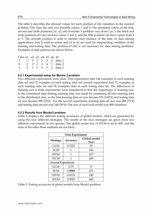
4.2.2 Results from Monks3 problem

Table 5 displays the different testing accuracies of global models, which are generated by

using the four different strategies. The results of the four strategies are given from two

different experiments in two groups. The global model size of WCM is set to 400, and the

sizes of the other three methods are not fixed.

First Experiment


Size

GCM 0.7222 39

SCM 1 196

MVM 1 167

WCM 1 400

Second Experiment

GCM 0.75 17

SCM 0.9583 276

MVM 0.8333 240

WCM 0.9583 400

Table 5. Testing accuracies of global models from Monk3 problem.

www.intechopen.com


275

The size of the training and testing data are the basic differences in these two experiments.

Here, accuracy of the first experiment is better than the accuracy of the second experiment.

In the first experiment, WCM, MVM and SCM attained 100% of accuracy. In the second

experiment, WCM and SCM have given better accuracy than other two strategies. The

Accuracy of MVM is significantly better in the first experiment than in the second

experiment. The accuracy of GCM in both experiments is poor.

Table 6 displays the testing accuracy of centralized learning model of both experiments. The

training iteration of centralized model was 5000 and the size of the learning model was set

to 400. These experiments help to compare the distributed data mining and centralized data

mining.

Centralized Model

Experiment Accuracy Learning Size

1 1 400

2 1 400

Table 6. Testing accuracies of Centralized model from Monk3 problem.

In centralized model, both experiments reached 100% of accuracy. In the first experiment,

the testing accuracies of the centralized model and the distributed model are similar, but in

the second experiment, the testing accuracy of the centralized model is better than the

testing accuracy of the distributed model.

4.3 ICU data

The Intensive Care Unit data is about the prediction of organ failure about 6 different

organic systems (M. Vilas-Boas, et al, 2010). The data have been collected from three distinct

sources: the electronic health record, ten bed side monitors, and paper based nursing record.

There is a total 31 fields of data in this problem. The data was collected from thirty two

patients’ information for first five days. The total number of records in this data set is 2107,

but this data was not balanced (the number of resulting ones and zeros were not equal).

Consequently, the data set was extracted for balancing the output. Hence the final data set

has 3566 records.

4.3.1 Experimental setup for ICU data

The ICU data was divided into two parts: 70% of the data was selected as training data and

the rest 30% was selected as testing data. Four different data sets with 624 records were

selected from the training data to make the four different training data sets in the

distributed sites. Similarly, four different data sets with 268 records were selected from the

testing data for four different testing data sets in the distributed sites. In the centralized data

mining, training data is made by combining all those four training data sets, so the training

data set size became 2496 (624*4), similarly testing data set was made by combining all those

four testing data sets, so the testing data set size became 1072 (268*4).

www.intechopen.com


276

4.3.2 Results from ICU data

Table 7 shows the different testing accuracies of global model, which are generated by using

the four different strategies used for constructing global model.

First Experiment


Size

GCM 0.84 1382

SCM 0.85 1466

MVM 0.89 1416

WCM 0.73 400

Table 7. Testing accuracies of global models from Monk3 problem.

The results showed in table 7 correspond to an interesting result when the ICU data is used.

The MVM has the best result but the GCM and SCM also are very close. Table 8 displays the

testing accuracy of centralized learning model. The training iteration of centralized model

was 5000 and the size of the learning model was set to 400.

Centralized Model

Experiment Accuracy Learning Size

1 0.68 400

Table 8. Testing accuracies of centralized model from ICU data.

The testing accuracy of CDM from ICU data is 0.68 (68%). In this problem, testing accuracy

of CDM has less accuracy than the testing accuracies of DDM. The global model sizes of

WCM and CDM are the same even though the testing accuracy of CDM is less than the

global model testing accuracy of WCM.

5. Discussion

Three axes will be considered to analyze the experimental results: 1. Significance of the training size; 2. Efficiency of different strategy for generating global model; 3. Comparison of DDM and CDM. The training data size affects the quality of models in the distributed sites. In monks 3

problem, training size of each node in the first experiment corresponds to double the

training size of each node in the second experiment; therefore, global model of the first

experiment is more general than the global model of the second experiment. That is why the

accuracy of the global model in the first experiment is better than the accuracy of the second

experiment.

www.intechopen.com


277

Now let’s examine the operating efficiency of each strategy used for making global model.

Here, less processing efficiency means that the processing time of the strategy is higher, and

more processing efficiency means those strategies need less processing time. The best

processing efficiency model is the WCM; because the WCM does not have any updates

(parameter modification) instead of it has only evaluation process (comparison). The

processing efficiency of SCM is lower than the WCM because SCM has not only the update

process, but also the evaluation process. The first process of the GCM and MVM is to

develop discrete classifier in the global model, up to SCM function. Hence the processing

efficiency of these two methods is lower than WCM and SCM. The GCM has less processing

efficiency than MVM because the GCM has two more processes after developing discrete

classifier, but the MVM has only one more process after the generation of discrete classifiers.

The global model of GCM and SCM represents all the local models. When the global model

is generated by WCM or MVM, some classifiers are removed from the global models. The

WCM keeps only the highest weighted classifiers in the global model therefore other

classifiers have to be removed from the global model. The number of classifiers kept in the

population is equal to the predefined size of the global model. In the MVM, the classifiers

which are above the threshold value are kept in the global model, other classifiers which are

less than the threshold value must be removed from the global model. The size of SCM is

bigger than those of all other methods and the accuracy of the global model also

comparatively better.

In the 11 multiplexer problems, centralized accuracy and distributed accuracy are almost

similar in both experiments. In the first experiment monks 3 problem centralized testing

accuracy and distributed testing accuracy are similar, but in the second experiment

centralized testing accuracy is better than the distributed testing accuracy.

Four main disadvantages of the CDM are: i, ii) the communication and computation are

higher; iii) less privacy of local data; and iv) the cost of implementation is higher. The

communicational cost of CDM is always higher because CDM has to send huge amount of

data from each distributed site to the central repository. Collected data in the central

repository would be very large therefore the computational cost of the CDM would be

higher (M. F. Santos, et al, 2010). There is some privacy issue to send private data of each

branch of the organization to central repository. Another constraint is that the cost of

implementation would be higher because the CDM requires high bandwidth

communicational channel for sending huge sized data, also very large sized storage

repository is required in the central repository because central repository has to store a large

size of data for centralized data mining. On the other hand, the DDM only needs to send the

local models from the distributed sites to the global site. The local model size would be very

smaller than the size of the processed data therefore the communicational cost is less. Data

mining is applied in every node in the distributed sites hence the computational cost of

DDM would be less than the computational cost of the CDM. In DDM, there is no privacy

issue because in DDM system doesn’t need to send data to central repository also the cost of

implementation is less because there is no need of high bandwidth communicational

channel and large size of storage device in the central repository. The main advantage of

CDM is that the global model of the centralized method represents the whole data set. So

the global model generated by the centralized method is more general than the global model

generated from the distributed method.

www.intechopen.com


278

6. Conclusions and future work

The main objective of this work is to find the benefits of the DDM relative to the CDM.

Above sections describe the benefits of the DDM, such as less implementation cost, less

communication cost, less computation cost, and no privacy issue. In addition to these

benefits, the accuracy of the global model in the DDM and the CDM are almost similar,

which means that we can change from CDM to DDM without losing accuracy. Therefore,

this work shows that DDM is the best method for implementing data mining in a

distributed environment.

Constructing and optimizing the global model was the second objective of this work that

describes and test four different strategies. The strategies of SCM and WCM achieved

accuracies that are close to those of CDM. Among those four strategies, GCM performed

worse.

The results also show that the size of the training data affect the quality of the models in the

Gridclass system.

Future work will address testing of bigger size of real world data. The communication and

computational cost of DDM and CDM would be included in the study for better

understanding of the performance of those two methods. Likewise further work would also

include more dynamic strategies to induced global model from the distributed local learning

model.

7. Acknowledgment

The authors would like to express their gratitudes to FCT (Foundation of Science and

Technology, Portugal), for the financial support through the contract

GRID/GRI/81736/2006.

8. References

A. Orriols-Puig, A Further Look at UCS Classifier System. GECCO’06, Seattle, Washington,

USA, 2006.

A. Orriols, EsterBernado-Mansilla, Class Imbalance Problem in UCS Classifier System:

Fitness Adaptation..,Evolutionary Computation, 2005. The 2005 IEEE congress on, 604-

611 Vol.1 2005.

A. Orriols, EsterBernado-Mansilla, Class Imbalance Problem in Learning Classifier System:

A Preliminary study. GECCO´05 Washington DC, USA, ACM 1-59593-097-3/05 2006,

2006

A. Meligy, M. Al-Khatib, A Grid-Based Distributed SVM Data Mining Algorithm.

European Journal of Scientific Research ISSN 1450-216X, Vol.27, No.3, pp313-321,

2009.

C. Clifton, M. Kantarcioglu, J. Vaidya, X. Lin, M. Y. Zhu, Tool for Privacy Preserving

Distributed Data Mining. Sigkdd Explorations volume 4, 2002.

G. Brown., T. Kovacs., J. Marshall., UCSpv: Principled Voting in UCS Rule Populations.

GECCO 2007, Genetic and Evolutionary Computation Conference proceeding of the 9th

annual conference on Genetic evolutionary computation, 2007.

www.intechopen.com


279

H. H. Dam, A scalable Evolutionary Learning Classifier System for Knowledge Discovery in

Stream Data Mining, M.Sci. University of Western Australia, Australia, B.Sci. (Hons)

Curtin University of Technology, Australia. Thesis work 2008.

H. Lu., E. Pi., Q. Peng., L. Wang., C. Zhang.,: A particle swarm optimization-aided fuzzy

cloud classifier applied for plant numerical taxonomy based on attribute similarity.

Expert system with applications, volume 36, pages 9388-9397 (2009).

I. Foster, The Anatomy of the Grid: Enabling Scalable Virtual Organizations, 1st International

Symposium on Cluster Computing and the Grid (CCGRID'01), Brisbane, Australia,

IEEE.

J. H. Holmes., P. L.. Lanzi., S. W. Wilson., W. Stolzmunn., Learning Classification System:

New Models Successful Applications., Information Processing Letters, 82 (23- 30),

2002.

J. Luo, M. Wang, J. Hu, Z. Shi, Distributed data mining on Agent Grid: Issues,

Platform and development toolkit. Future Generation computer system 23, 61-68,

2007.

K. Shafi, T. Kovacs, H. A. Abbass, W. Zhu, Intrusion detection with evolutionary learning

classifier system. Springer Science+ Business Media B. V. 2007.

M. F. Santos, W. Mathew, T. Kovacs, H. Santos, A grid data mining architecture for learning

classifier system. WSEAS TRANSACTIONS on COMPUTERS Volume 8, ISSN: 1109-

2750 2009.

M. F. Santos, W. Mathew, H. Santos, GridClass: Strategies for Global Vs Centralized Model

Construction in Grid Data Mining. Workshop on Ubiquitous Data Mining, Artificial

Intelligence (ECAI2010), in Portugal, 2010.

M. F. Santos, H. Quintela, J. Neves, Agent-Based learning Classifier System for Grid Data

Mining. . GECCO, Seattle, WA, USA 2006.

M. F. Santos. Learning Classifier System in Distributed environments, University of Minho

School of Engineering Department of Information System. PhD Thesis work 1999.

M.Cannataro, A. Congiusta, A. Pugliese, D.Talia, P. Trunfio, Distributed Data Mining on

Grid: Services, Tools, and Applications. IEEE TRANSACTIONS ON SYSTEM,

MAN, AND CYBERNETICS- PART B: CYBETNETICS, VOL. 34 NO6, DECEMBER

2004.

M. Plantie., M. Roche., G. Dray., P. Poncelet.,: Is voting Approach Accurate for Opinion Mining?

Proceedings of the 10th international conference on Data Warehousing and Knowledge

Discovery 2008.

M. Vilas-Bous, M. F. Santos, F. Portela, A. Silva, F. Rua, Hourly prediction of organ failure

and outcome in intensive care based on data mining techniques. ICEIS 2010

conference, 2010.

M. Y. Santos., A. Moreira., Automatic Classification of Location Contexts with Decision

Tree. Proceeding of the Conference on Mobile and Ubiquitius System, 2006.

N. Zhang, H. Bao, Researchon Distributed Data Technology Based on Grid. First

International Workshop on Database Technology and Applications 2009.

T. Kovacs, Strength or Accuracy: Credit Assignment in Learning Classifier

Systems. Distinguished Dissertation,. Springer-Verlag London limited, page 26,

2004.

www.intechopen.com


280

V. Stankovski, M. Swain, V. Kravtsov, T. Niessen, D. Wegener, J. Kindermann, W. Dubitzky,

Grid-enabling data mining applications with DataMiningGrid: An Architectural

perspective. Future Generation Computer System24, 256- 279, 2008.

www.intechopen.com

New Fundamental Technologies in Data MiningEdited by Prof. Kimito Funatsu

ISBN 978-953-307-547-1Hard cover, 584 pagesPublisher InTechPublished online 21, January, 2011Published in print edition January, 2011

InTech EuropeUniversity Campus STeP Ri Slavka Krautzeka 83/A 51000 Rijeka, Croatia Phone: +385 (51) 770 447 Fax: +385 (51) 686 166www.intechopen.com

InTech ChinaUnit 405, Office Block, Hotel Equatorial Shanghai No.65, Yan An Road (West), Shanghai, 200040, China

Phone: +86-21-62489820 Fax: +86-21-62489821

The progress of data mining technology and large public popularity establish a need for a comprehensive texton the subject. The series of books entitled by "Data Mining" address the need by presenting in-depthdescription of novel mining algorithms and many useful applications. In addition to understanding each sectiondeeply, the two books present useful hints and strategies to solving problems in the following chapters. Thecontributing authors have highlighted many future research directions that will foster multi-disciplinarycollaborations and hence will lead to significant development in the field of data mining.

How to referenceIn order to correctly reference this scholarly work, feel free to copy and paste the following:

Henrique Santos, Manuel Filipe Santos and Wesley Mathew (2011). Supervised Learning Classifier System forGrid Data Mining, New Fundamental Technologies in Data Mining, Prof. Kimito Funatsu (Ed.), ISBN: 978-953-307-547-1, InTech, Available from: http://www.intechopen.com/books/new-fundamental-technologies-in-data-mining/supervised-learning-classifier-system-for-grid-data-mining

© 2011 The Author(s). Licensee IntechOpen. This chapter is distributedunder the terms of the Creative Commons Attribution-NonCommercial-ShareAlike-3.0 License, which permits use, distribution and reproduction fornon-commercial purposes, provided the original is properly cited andderivative works building on this content are distributed under the samelicense.

https://creativecommons.org/licenses/by-nc-sa/3.0/

supervised learning classifier system for grid data mining

Documents