Intensified summer monsoon and the urbanization of Indus Civilization in

northwest India

Yama Dixit1,2, David A. Hodell1, Alena Giesche1, Sampat K. Tandon4, Fernando Gázquez1,3, Hari S. Saini5, Luke Skinner1, Syed A.I. Mujtaba5, Vikas Pawar6, Ravindra N. Singh7, Cameron A. Petrie8

1Godwin Laboratory for Palaeoclimate Research, Department of Earth Sciences, University of Cambridge, Cambridge, CB2 3EQ, United Kingdom2IFREMER, Unité de Recherche Géosciences Marines, Z.I. Pointe du Diable, BP 70, 29280 Plouzané, France3School of Earth and Environmental Sciences, University of St. Andrews, UK4Department of Earth and Environmental Sciences, IISER Bhopal, India5Geological Survey of India, Faridabad, India6 Department of History, Maharshi Dayanand University, Rohtak, Haryana, India7 Department of AIHC and Archaeology, Banaras Hindu University, Varanasi, India8Department of Archaeology, University of Cambridge, Cambridge, CB2 3DZ, United Kingdom

Corresponding author E-mail address: yamadixit@gmail.com

1

Supplementary information

OSL dating methodology

The middle part from each sample tube was selected to determine the depositional

ages by OSL technique 1. The outer parts were used for dose rate and water content

measurements. A selected portion was treated with 1N HCl solution to remove the

carbonates and 30% H2O2 to remove organic impurities. The dried sediments were

sieved to separate a 90-150 μm grain size fraction from which quartz grains were

separated using a sodium polytungstate solution of 2.58 g/cm3 specific density. The

20 μm outer layer of quartz grains was removed by etching with 40% HF for 80

minutes and then by HCL for 20 minutes. This was done to remove feldspars and the

alpha irradiated layer. The quartz grains were temporarily mounted on stainless steel

discs (9.6 mm diameter) as a monolayer, generally over a circular area of 4 mm

diameter with the help of silicon spray. Luminescence measurements were carried out

using a Risoe TL/OSL Reader 15-20 DA, equipped with a calibrated Sr-90 beta

source. The stimulation was made using blue LED’s (470±30 nm) and the

luminescence was detected in the UV range through a Hoya UV-340 filter placed in

front of an EMI9671 photomultiplier tube. Luminescence was recorded in 250

channels (40 s) in which counts of first five channels were considered for further

calculation after subtracting background counts of the last 25 channels. The aliquot

discs were placed in alternating holes of the sample carousel to avoid

irradiation/stimulation crosstalk. Generally four pre-dating tests were conducted on

each sample before actual measurement of De. These included feldspar screening,

2

rough dose estimation, preheat plateau test and dose recovery test. When feldspar

signals were recorded, the sample was retreated with HF. Generally the IRSL/OSL

ratio was kept below 1%. Nevertheless, an additional step of IRSL at 75°C per sec for

100 sec was given before each blue OSL measurement. Blue light stimulation was

carried out at 125°C for 40 s. A preheat temperature of 220°C for 10 s and TL of

180°C (in-lieu of preheat) were found suitable. The heating rate used was 5°C/s. The

dose recovery was within ±10% of the administered dose. The equivalent dose (De)

was measured following the Single Aliquot Regeneration (SAR) protocol 2,3.Sample

discs with recycling ratio within 10% and recuperation of less than 5% were

considered for final calculation of the De values. The commercial software “Analyst”

was used for the calculation of individual De values. Calculation of De’s was repeated

from the spreadsheets provided by A.S. Murray, Risoe National Laboratory,

Denmark. It was found that average De values of well bleached samples were similar

in both calculations. The spreadsheets were helpful in discriminating the recuperation,

sensitivity changes and recycling ratio. The samples had near normal distribution of

De values, therefore, weighted averages were employed for age calculation using

Grun software. The dose rates (Dr) of samples were calculated from the concentration

of U and Th (analyzed by ICP-MS) and K (by flame photometer at Chemical Labs,

GSI, Faridabad). The OSL ages are compiled in Table 1.

Isotope mass balance model for Unit III gypsum deposition

As described in the main text, paleolake Karsandi was a closed basin during the

Holocene and the only significant water loss from the lake was through the process of

3

evaporation. The change in oxygen isotope ratios from a drying water body can be

described by the Craig-Gordon equation4, which takes into account evaporation and

the changing isotopic composition between lake and atmospheric water in similar

lines as Dixit et al., 20165. The assumption made in the calculations is that the water

loss results from evaporation and that the conditions of evaporation (e.g., temperature,

relative humidity) remained unchanged. The evolution of oxygen isotope ratios as a

function of fraction of residual lake water with progressive evaporation is calculated

from the following relationship 6:

where δ0 is the initial isotopic composition of water, f is the fraction of residual water

in the lake, A/B is the isotopic composition that water attains in its final evaporation

stages when f approaches zero and A and B are:

δa is the δ18O of the atmosphere, which can be calculated from the ambient

temperature in Karsandi as, δ18O = 0.39T (C) – 22.8;

Given the average annual temperature range at Karsandi, 17 to 33°C, the calculations

were performed at 25°C, aw is the thermodynamic activity of water: aw = -0.000543/f2 -

0.018521/f + 0.99931; h is the fractional relative humidity, taken as h/aw that changes

with lake volume; ∆, the kinetic enrichment factor: ∆= 0.0142 (1-h/aw); is the

4

equilibrium fractionation factor: = exp (1137/T2 - 0.4156/T- 0.00207) 7; T is the

temperature in Kelvin; is total isotopic enrichment factor: = -1

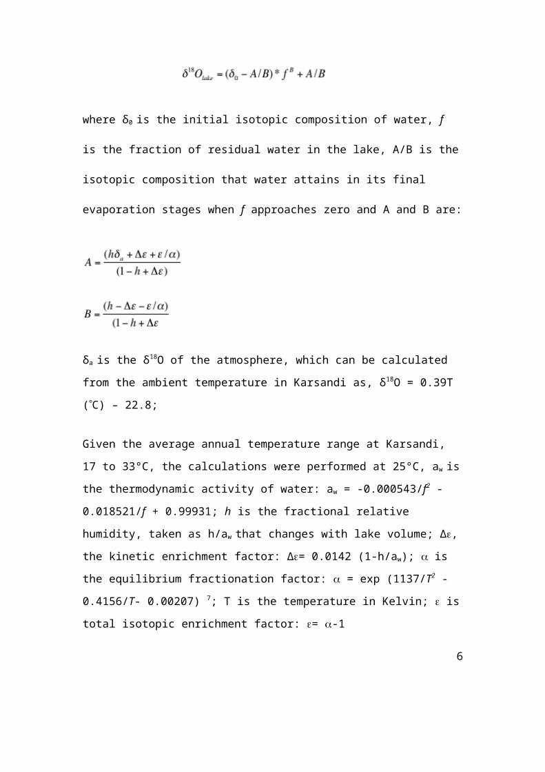
We evaluate two possible scenarios firstly for Unit III deposition (Case I) and

secondly for the deposition of massive gypsum (Case II).

Case I: When the summer monsoon rain was higher than today (in blue). We

take the initial composition of lake water, δ0 = -10, the present day isotopic

composition of the summer rain.

Case II: When the summer monsoon rainfall was much lower (in red) and

therefore initial composition of lake water δ0 = -7, which is about the present day

isotopic composition of the groundwater in Karsandi (obtained from the intersection

of Karsandi evaporative line and the local meteoric water line as described in the main

text).

Using these two initial composition of lakewater as the starting point, the calculations

for the evolution of δ18O in the lake water were carried out until f = 0.2. The δ18O in

the lake water obtained by evaporation of lake water until the remaining volume

changed from 100 to 20%, is ~3‰, which is about the average δ18O of Unit III and is

lower than the δ18O of gypsum units.

5

Supplementary Figure 1

6

Figure S1. The top image shows a panoramic view of the location of paleolake

Karsandi deposits (N28°59’29.6: E74°45’53.8) from Nohar-Bhadra district in the

Indian state of Rajasthan on the Thar Desert margin in northwest India. The red

rectangle denotes the approximate size of the section sampled for this study. Bottom

figure shows the lithology of Karsandi paleolake section sampled (this study) and

corresponding units (A1, A2, F1-F3) as described by Saini et al (2005)8. Position of

radiocarbon levels are denoted by red triangles and OSL dates in blue. Unit I- Yellow-

brown Aeolian sand; Unit II- Massive gypsum deposits; Unit III- silty sand with

nodular gypsum and ostracods and gastropods, Unit IV- Massive gypsum; Unit V-

Interbedded sand with gypsum; Unit VI- Massive gypsum; Unit VII Interbedded sand

with gypsum lenses; Unit VIII- Massive gypsum deposits. The lacustrine deposits

7

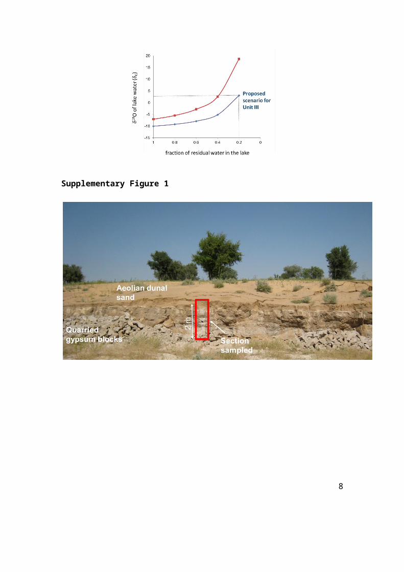
from Unit I-VIII are underlain by yellow brown aeolian sand.Supplementary Figure

2:

8

Figure S2: (A) Location of samples taken for OSL dating located just above the

topmost gypsum unit at 40 cm; (B) Location of OSL date sample taken from the

aeolian sands underlying the lowermost gypsum unit at 230 cm.

9

Supplementary Figure 3

Figure S3. Schematic cross-section of an ephemeral playa (using CorelDRAW X6

software). (A) During periods of reduced monsoon, a shallow saline pond is

maintained at gypsum saturation throughout the year through groundwater inflow to

the playa basin and high evaporation rates, resulting in massive continuous gypsum

deposits. (B) In contrast, periods of greater monsoon rainfall results in groundwater

and surface flow into the lake in summer transporting detrital sediments followed by

gypsum formation during the dry season.

Supplementary Figure 4

10

Figure S4. XRD results of (A) bulk sediment sample from a typical gypsum unit from

Karsandi, Unit II (10-12 cm) showing 2-theta peak of gypsum. (B) bulk sediment

sample from Unit III (12-14 cm) showing 2-theta peak of gypsum (G), calcite (C) and

quartz (Q). The reference peak positions and intensities are from the PDF2 database.

11

Mineral identification was aided by the use of an automated search-match computer

program9.

12

Supplementary Figure S5

Figure S5. Karsandi age model obtained using BACON program based on flexible

Bayesian age modeling 10. The top and bottom OSL dates are shown in light blue

colour. The radiocarbon dates were calibrated using the IntCal13 calibration curve 11.

13

Figure S6. 18O and D values of lake water plotted vs BACON model ages. Grey

bands show the gypsum units. The wettest period suggested by high 18O and D

values occurs between ~5.2 and ~4.4 ka BP. High 18O and D values indicating arid

conditions (shown in red bar) has a median age of ~4.1 ± 0.1 ka BP, which is

coincident with the timing of Indus de-urbanization 12. Also shown are the high lake

level period (rectangles in blue) and timing of permanent decline of lake levels

(indicated by red dashed line) in other Thar Desert lakes from west to east, Lakes Bap

Malar 13 and Lunkaransar 14 on the western margin dried up first followed by Didwana 15, Karsandi and finally Sambhar 16. The numerals indicate ages in ka BP.

14

Supplementary Figure S7

Figure S7: Percent gypsum (green), % detrital (red) and % calcium carbonate (black)

from paleolake Karsandi. Yellow horizontal bars denote the gypsum units VIII, VI,

IV and II.

15

Supplementary Figure S8

Figure S8: Uncorrected 18O and D of gypsum hydration water from Karsandi

profile. Error bars show 1 based on the 18O and D results for the internal

gypsum standard NewGyp 17.

16

References:

1. Aitken, M. J. Introduction to optical dating: the dating of Quaternary

sediments by the use of photon-stimulated luminescence. (Clarendon Press,

1998).

2. Murray, A. S. & Roberts, R. G. Measurement of the equivalent dose in quartz

using a regenerative-dose single-aliquot protocol. Radiat. Meas. 29, 503–515

(1998).

3. Murray, A. S. & Wintle, A. G. Luminescence dating of quartz using an

improved single-aliquot regenerative-dose protocol. Radiat. Meas. 32, 57–73

(2000).

4. Craig, H. & Gordon, L. I. Deuterium and oxygen 18 variations in the ocean and

the marine atmosphere. (1965).

5. Dixit, Y., Hodell, D. A., Sinha, R. & Petrie, C. A. Oxygen isotope analysis of

multiple, single ostracod valves as a proxy for combined variability in seasonal

temperature and lake water oxygen isotopes. J. Paleolimnol. 53, 35–45 (2015).

6. Gonfiantini, R. Environmental isotopes in lake studies. Handb. Environ. Isot.

Geochemistry; Terr. Environ. 113–168 (1986).

7. Majoube, M. Fractionnement en oxygene 18 et en deuterium entre l’eau et sa

vapeur. J. Chim. Phys. 68, 1423–1436 (1971).

17

8. Saini, H. S., Tandon, S. K., Mujtaba, S. A. I. & Pant, N. C. Lake deposits of the

northeastern margin of Thar Desert: Holocene(?) Palaeoclimatic implications.

Curr. Sci. 88, 1994–2000 (2005).

9. Marquart, M., Deisenhofer, J., Huber, R. & Palm, W. Crystallographic

refinement and atomic models of the intact immunoglobulin molecule Kol and

its antigen-binding fragment at 3.0 Å and 1.9 Å resolution. J. Mol. Biol. 141,

369–391 (1980).

10. Blaauw, M. & Christen, J. A. Flexible paleoclimate age-depth models using an

autoregressive gamma process. Bayesian Anal. 6, 457–474 (2011).

11. Reimer, P. J. et al. IntCal13 and Marine13 radiocarbon age calibration curves

0–50,000 years cal BP. Radiocarbon 55, 1869–1887 (2013).

12. Dixit, Y., Hodell, D. A. & Petrie, C. A. Abrupt weakening of the summer

monsoon in northwest India ~4100 yr ago. Geology 42, 339–342 (2014).

13. Deotare, B. C. et al. Palaeoenvironmental history of Bap-Malar and Kanod

playas of western Rajasthan, Thar desert. J. Earth Syst. Sci. 113, 403–425

(2004).

14. Enzel, Y. et al. High-resolution Holocene environmental changes in the Thar

Desert, northwestern India. Science (80-. ). 284, 125–128 (1999).

15. Singh, G., Wasson, R. & Agrawal, D. Vegetational and seasonal climatic

18

changes since the last full glacial in the Thar Desert, northwestern India. Rev.

Palaeobot. Palynol. 64, 351–358 (1990).

16. Sinha, R. et al. Late Quaternary palaeoclimatic reconstruction from the

lacustrine sediments of the Sambhar playa core, Thar Desert margin, India.

Palaeogeogr. Palaeoclimatol. Palaeoecol. 233, 252–270 (2006).

17. Gázquez, F., Evans, N. P. & Hodell, D. A. Precise and accurate isotope

fractionation factors (α17O, α18O and αD) for water and CaSO4·2H2O

(gypsum). Geochim. Cosmochim. Acta 198, 259–270 (2017).

19