supplementary online content - jama psychiatry · supplementary online content sun h, lui s, yao l,...

© 2015 American Medical Association. All rights reserved.

Supplementary Online Content

Sun H, Lui S, Yao L, et al. Two patterns of white matter abnormalities in medication-naive patients with

first-episode schizophrenia revealed by diffusion tensor imaging and cluster analysis. JAMA Psychiatry.

Published online May 20, 2015. doi:10.1001/jamapsychiatry.2015.0505.

eAppendix. Methods

eFigure 1. Flowchart That Illustrates Analytic Procedures for the DTI Data

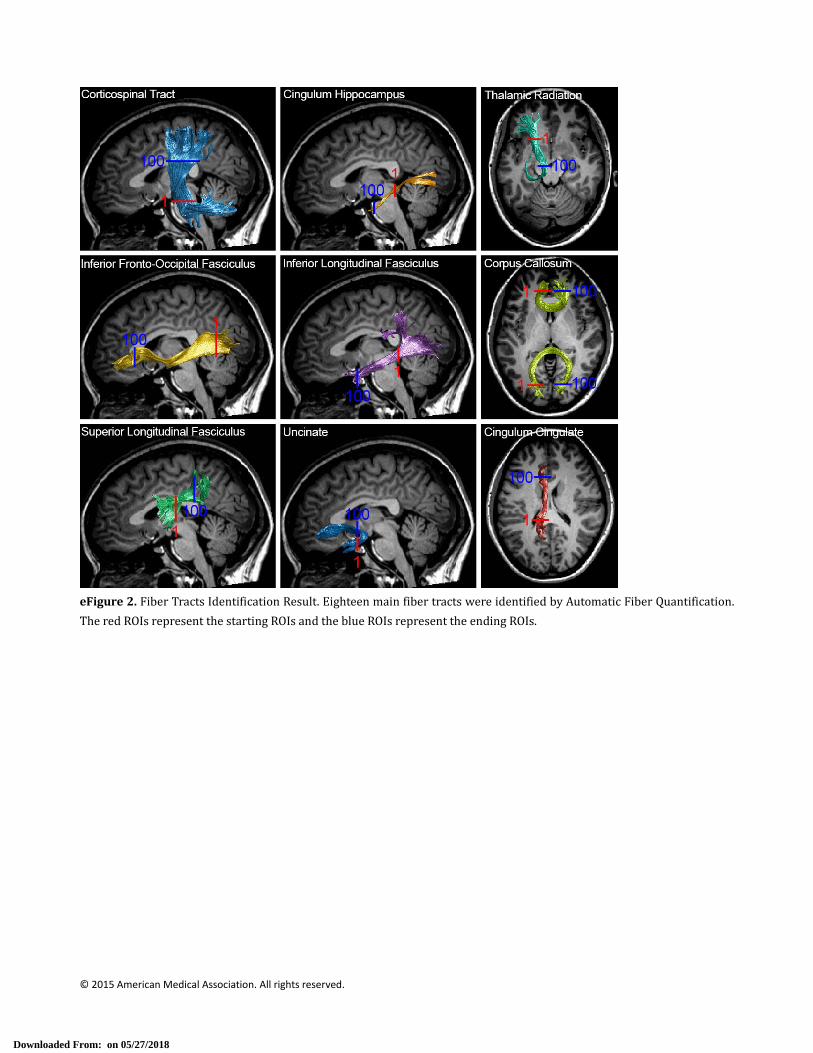
eFigure 2. Fiber Tracts Identification Result

eFigure 3. Flowchart for Pointwise Comparison

eFigure 4. Cluster Validation to Determine the Optimal Cluster Number

eFigure 5. Stability Test Based on Subsampling Technique and Comparison With Randomly Generated Data

eTable 1. Comparison of Mean FA Between Healthy Controls and Patient Subgroups Across 18 Fiber Tracts

eTable 2.Comparison of Mean MD Between Healthy Controls and Patient Subgroups Across 18 Fiber Tracts

eReferences

This supplementary material has been provided by the authors to give readers additional information about their

work.

Downloaded From: on 05/27/2018


eAppendix. Methods

1. Participants

One hundred and thirteen right‐handed first‐episode schizophrenia patients (56 male, 57 female, age from 16 to 46, mean

age 23.8) recruited from inpatient units of the Mental Health Center, West China Hospital, Sichuan University were

included in this study. Diagnosis was determined using the Structured Clinical Interview for DSM‐IV (SCID), and clinical

symptoms were assessed using the Positive and Negative Syndrome Scale (PANSS). Illness duration of all patients was less

than 2 years, with illness onset evaluated by the Nottingham Onset Schedule1 using information provided by patients,

family members and other sources when available.

Healthy controls (58 male, 52 female, age from 18 to 41, mean age 23.4) were recruited from the local community via

poster advertisements. None had a history of psychiatric disorder determined by the SCID interview, and none had

first‐degree relatives had a known history of a psychotic disorder. Patients and controls were matched in terms of age, sex,

years of education, and handedness between schizophrenia patients and healthy controls (all p>0.05). All participants had

no current or past history of substance abuse or dependence as assessed by SCID.

This study was approved by the Ethics Committee of West China Hospital. Written informed consent was obtained

from each participant before study participation.

2. Magnetic resonance imaging acquisition

All magnetic resonance imaging scans were performed using a GE Signa EXCITE 3.0T scanner (GE healthcare, Milwaukee,

Wisconsin) equipped with an 8‐channel phase array head coil. The DTI data was acquired using a bi‐polar diffusion

weighted spin‐echo echo planar imaging (EPI) sequence (TR=10000ms, TE=70ms) with 128 x 128 matrix over a field of view

of 240 x 240 mm and 42 axial slices of 3 mm thickness to cover the whole brain without gap. Each DTI dataset included 20

images of unique diffusion directions at b=1000s/mm2 and a non‐diffusion image (b=0). High resolution T1 weighted

anatomical images were acquired for registration purposes using a 3D spoiled gradient (3D‐SPGR) sequence (TR=8.5ms,

TE=3.5ms, TI=400ms, Flip angle=12) with 240 x 240 matrix over a field of view of 240 x 240 mm and 156 axial slices of

1mm thickness. All scans were reviewed by an experienced neuroradiologist to exclude gross brain abnormalities.



3. DTI processing and automatic tracts identification

Raw DTI images were preprocessed using FSL software (FMRIB Software Library, FMRIB, Oxford, UK)2. For each DTI

dataset, all diffusion weighted images were affinely coregistered to the b0 image using FLIRT (FMRIB’s Linear Image

Registration Tool)3 with 12 degree of freedom so as to correct for eddy current induced distortion and subtle head

motion. The rotational component of the transformation matrix was extracted for each volume to adjust the

diffusion gradient encoding table. A brain mask was created from the b0 image using BET (Brain extraction Tool)4 with

fractional intensity threshold equal to 0.2. FDT (FMRIB’s Diffusion Toolbox) was used to fit the tensor model with the

adjusted gradient encoding table.

For fiber tract identification, we used a Matlab‐based open source software Automatic Fiber Quantification

(AFQ),5 which implemented both fiber tracts identification algorithms proposed by Hua et al.6 and Zhang et al.7. The

identification procedure included three primary steps. Firstly, whole brain deterministic fiber tracking was performed

on preprocessed tensor images using a streamline tracking algorithm with a fourth‐order Runge‐Kutta path

integration method.8 The tracking algorithm starts within a white matter mask defined as voxels with FA value

greater than 0.3, then the path integration procedure traces the fiber in both directions along principal diffusion axes.

The tracing is terminated when the FA value becomes lower than 0.2 or the minimum angle between the last path

segment and next step is greater than 30°. Secondly, fiber tract segmentation was performed using the waypoint ROI

procedure described by Wakana et al.9 The waypoint ROI sets developed at the John Hopkins Medical Institute

(http://cmrm.med.jhmi.edu/) were warped from the MNI template space into individual coordinate space via

non‐linear transformation. Each fiber was defined as a candidate to a particular fiber group if it passed through two

waypoint ROIs that define a specific fiber tract. Finally, fiber refinement was accomplished by comparing each

candidate fiber to fiber tract probability maps develop by Hua et al.6 The fiber tract probability maps were also

registered to each individual space and then candidate fibers for a particular fiber group were assigned scores

according to probability values of the voxels they pass through. If a candidate fiber does not get the highest

probability score to the same fiber group, it was judged to have an aberrant trajectory and would be discarded.



Additionally, an iterative procedure was used to remove fibers that were much longer or shorter than the mean fiber

length or far from the core of the fiber tract and finally form a compact fiber bundle. Eighteen fiber tracts were

identified according to the predefined ROIs and probability maps: bilateral anterior thalamic radiation, corticospinal

tract (CST), cingulum cingulate, cingulum hippocampus, inferior fronto‐occipital fasciculus (IFOF), inferior longitudinal

fasciculus (ILF), superior longitudinal fasciculus (SLF), uncinate, genu and splenium of corpus callosum.

4. Feature extraction, cluster analysis and cluster validation

Feature extraction

After tract identification, the portion of fibers between two waypoint ROIs was clipped. The fiber tract core is

calculated by resampling each clipped fiber into 100 equidistant nodes and calculating the mean location of each

node. Diffusion measurements are calculated at each node on fiber core by calculating the weighted average of the

diffusion properties of each clipped fiber at corresponding node. The weighting was determined based on the

Mahalanobis distance of each fiber node from the fiber core. The diffusion measurement along the fiber tract core,

which is a vector of 100 values, was defined as the tract profile. In addition to FA, the tract profile of mean diffusivity

(MD), a summative measure that describes average total diffusivity in a given voxel,10 was also evaluated because

previous studies observed MD increased in white matter of schizophrenia patients.11 The resulted tract profiles were

visually inspected to exclude subjects with obvious calculation error in fiber reconstruction or identification.

Before feature extraction, both FA and MD profiles were first smoothed using 10‐point moving average to

reduce local dramatic variation caused by imaging noise. As only monotone FA or MD changes have been reported in

previous DTI studies, we defined the integration of FA and MD values along the full length of profiles as the features

of a tract. In this way, each tract had two features and each subject would have 36 features to depict their global

white matter status. The use of tract‐based feature extraction method has advantages over existed pattern

classification studies using DTI data, which adopted voxel information from warped FA maps followed by

dimensionality reduction techniques such as principle component analysis (PCA).12,13 The voxel‐based feature

extraction scheme is susceptible to alignment error. Moreover, the anatomical information attached to voxels is



discarded after dimensionality reduction, which makes it difficult to further locate the abnormalities. In contrast, the

tract‐based method was performed in individual coordinate space, thus relatively insensitive to alignment error and

anatomical variation.

Cluster analysis

The next step was to perform a cluster analysis in the schizophrenia patients using the 36 numerical white

matter feature extracted above. As the number of subgroups in schizophrenia patients is unknown, hierarchical

clustering was performed as it does not require cluster number as a prior input.14 Agglomerative hierarchical

clustering was done with in‐house Matlab code. Each feature was normalized into range of (‐1, 1) before fed into

clustering procedure. Euclidean distance was used as the distance metric between subjects, and average distance

between clusters was used as the linkage function. In the clustering procedure, Euclidean distance was first

calculated between subjects, and then pairs of subjects that were in close proximity were linked into binary clusters.

The newly formed clusters were grouped into larger clusters in an iterative way until a hierarchical tree was formed.

Cluster validation

To determine the optimal cluster number, the following indices: Silhouette index15, Dunn Index16 and Connectivity17, which

reflect the compactness, separation and connectedness, were employed in this study.

Silhouette index is the mean Silhouette width of all the samples and it reflects the compactness and separation of

clusters. The Silhouette width s of a sample is defined as:

max ,

Where a represents the average distance of a sample from the other samples of the cluster to which the sample is

assigned, and b represents the minimum of the average distance of the sample from samples of the other clusters. The

value of Silhouette index varies from ‐1 to 1 and higher value indicates better clustering result.

Dunn index is the ratio of the smallest distance between samples not in the same cluster to the largest intra‐cluster

distance. It is computed as



min min,

,max ∆

Where m is the number of clusters, δ , is the inter‐cluster distance between clusters and ,

∆ max , ∈ , is the maximum distance between two samples within same cluster. The Dunn index has a

value between zero and ∞. Larger values of Dunn index correspond to better cluster quality and the number of clusters

that maximizes the Dunn index is taken as the optimal number of clusters.

The Connectivity is defined as

,

for a particular clustering partition of N samples into m clusters, Define as the jth nearest neighbor of sample i, and

let , be zero if i and j are in the same cluster and 1 ⁄ otherwise. L is a parameter giving the number of nearest

neighbors to use. This index is capable of detecting the appropriate clusters with any shape, size or convexity as long as

they are separated. The connectivity has a value between zero and 1 and should be minimized for achieving the proper

clustering.

Above three indices were measured by cutting the dendrogram into 2 to 10 clusters. Silhouette and Dunn index reach

maximum and connectivity reaches minimum when cluster number equals to 2 (eFigure 4). Thus the optimal cluster

number that best represents the data structure is 2.

Cluster algorithm tends to generate clusters even if the data has no inherent cluster structure. We employ a

subsampling method proposed by Ben‐Hur et al.18 to validate the stability of cluster result. The general idea about stability

of clusters is that when a partition has captured the structure in the data, this partition should be stable with respect to

perturbation of the data. The method is implemented as follows: the whole dataset is clustered; a set of random

subsamples (75% of whole dataset) is generated and clustered as well. For increasing values of cluster number m, the

similarity between partitions of the whole dataset into m clusters and partitions of the subsamples are calculated. When

the structure in the data is well represented by m clusters, the partition of the whole dataset will be highly similar to

partitions of the subsampled data. To comparison with dataset without inherent cluster structure, ten random datasets



with same size with our original datasets and with each diffusion parameter randomly sampled from a normal distribution

with same mean and standard deviation of original data were generated. The plot of similarity versus cluster number

shows our data reach maximum similarity (0.97) when cluster number equal to 2, which indicate two‐cluster partition

scheme is most stable (eFigure 5). The curve derived from randomly generated dataset showed low similarity (around 0.4)

in all possible cluster numbers. The difference behavior between the curves derived from real dataset and random

datasets confirmed our data did have inherent cluster structure.



eFigure 1. Flowchart That Illustrates Analytic Procedures for the DTI Data. Red rectangles represent data while blue

rectanglesrepresentoperationsperformedonthem



eFigure2.FiberTractsIdentificationResult.EighteenmainfibertractswereidentifiedbyAutomaticFiberQuantification.

TheredROIsrepresentthestartingROIsandtheblueROIsrepresenttheendingROIs.



eFigure3. Flowchart forPointwiseComparison.The tractprofiles froma subjectwerearranged in a singlematrix.All

thesematrixeswere fed intopermutation‐based statistical analysiswith10000permutationsusing theFSLRandomize

program with age and illness duration as covariates. The statistical results were subject to family‐wise error (FWE)

correctionformultiplecomparisonsfollowingthreshold‐freeclusterenhancement(TFCE)andthresholdedbyp<0.05and

finallydisplayedasbarsundereachtractprofileplot.



eFigure4.ClusterValidationtoDeterminetheOptimalClusterNumber.Theplotsofvalidityindicesversusthenumberof

clusters from2 to10.Our cluster result reaches themaximum forSilhouette index (0.51),Dunn index (19.25) and the

minimum for connectivity (2.93) when cluster number equals to 2, suggesting the optimal cluster number that best

representsthedatastructureis2.



eFigure5. Stability Test Based on Subsampling Technique and ComparisonWith Randomly Generated Data (Red line

representsourrealdata;bluelinesrepresentrandomlygenerateddata).Ourdatareachesthehighestaveragesimilarity

(0.97)betweenwholedatasetandsubsampleddatasetswhenclusternumberequalsto2.



eTable 1. Comparison of Mean FA Between Healthy Controls and Patient Subgroups Across 18 Fiber Tracts

Subgroup 1 Subgroup2 Healthy control

ANOVA Post hoc*

F P Subgroup 1 vs HC P Subgroup2 vs HC P

L. ATR 0.4646±0.0349 0.4754±0.0242 0.4812±0.0320 5.27 0.0058 0.0027 0.4685

R. ATR 0.4736±0.0303 0.4824±0.0208 0.4861±0.0275 4.06 0.0186 0.0098 0.6464

L. CST 0.6102±0.0288 0.6219±0.0259 0.6214±0.0280 4.59 0.0111 0.0093 0.8695

R. CST 0.5956±0.0275 0.6089±0.0277 0.6110±0.0284 6.06 0.0028 0.0018 0.8806

L. CCing 0.4395±0.0613 0.4637±0.0472 0.4704±0.0517 6.71 0.0016 0.0011 0.9337

R. CCing 0.4201±0.0349 0.4355±0.0463 0.4425±0.0415 5.41 0.0051 0.0029 0.7723

L. CHipp 0.3853±0.0409 0.4238±0.0466 0.4312±0.0426 22.1 <0.0001 0.0029 0.5308

R. CHipp 0.4039±0.0362 0.4447±0.0329 0.4546±0.0453 31.07 <0.0001 <0.0001 0.2693

CC Splenium 0.5995±0.0586 0.6327±0.0266 0.6302±0.0494 9.40 0.0001 0.0003 0.9412

CC Genu 0.5982±0.0306 0.6274±0.0269 0.6347±0.0332 26.68 <0.0001 <0.0001 0.3031

L. IFOF 0.4931±0.0308 0.5110±0.0314 0.5168±0.0331 10.41 <0.0001 <0.0001 0.4823

R. IFOF 0.4781±0.0287 0.5029±0.0258 0.5087±0.0318 20.85 <0.0001 <0.0001 0.4366

L. ILF 0.4491±0.0296 0.4826±0.0358 0.4846±0.0333 24.11 <0.0001 <0.0001 0.9205

R. ILF 0.4140±0.0278 0.4434±0.0292 0.4498±0.0298 29.42 <0.0001 <0.0001 0.3492

L. SLF 0.4297±0.0318 0.4379±0.0407 0.4575±0.0445 9.73 0.0001 <0.0001 0.0105

R. SLF 0.4210±0.0273 0.4481±0.0437 0.4557±0.0425 17.30 <0.0001 <0.0001 0.0815

L. Uncinate 0.4352±0.0378 0.4727±0.0426 0.4668±0.0414 15.07 <0.0001 <0.0001 0.6301

R. Uncinate 0.4139±0.0347 0.4438±0.0337 0.4484±0.0329 20.88 <0.0001 <0.0001 0.6529

eTable 2. Comparison of Mean MD Between Healthy Controls and Patient Subgroups Across 18 Fiber Tracts

Subgroup 1 Subgroup 2 Healthy control

ANOVA Post hoc*

F P Subgroup 1 vs HC P Subgroup 2 vs HC P

L. ATR 0.7163±0.0209 0.7008±0.0218 0.7023±0.0277 7.62 0.0006 0.0013 0.9127

R. ATR 0.7222±0.0234 0.7054±0.0236 0.7074±0.0216 10.20 <0.0001 0.0002 0.8335

L. CST 0.7074±0.0238 0.6894±0.0185 0.6884±0.0218 15.96 <0.0001 <0.0001 0.9592

R. CST 0.7061±0.0211 0.6927±0.0191 0.6897±0.0174 14.42 <0.0001 <0.0001 0.5868

L. CCing 0.7356±0.0318 0.7106±0.0347 0.7148±0.0370 6.49 0.0018 0.0046 0.7795

R. CCing 0.7032±0.0263 0.6848±0.0369 0.6886±0.0306 4.26 0.0153 0.0311 0.7641

L. CHipp 0.7619±0.0366 0.7395±0.0298 0.7403±0.0345 8.95 0.0002 0.0003 0.9881

R. CHipp 0.7664±0.0292 0.7309±0.0293 0.7341±0.0304 27.41 <0.0001 <0.0001 0.7733

CC Splenium 0.8175±0.0525 0.7893±0.0378 0.7834±0.0751 6.01 0.0029 0.0017 0.8130

CC Genu 0.7859±0.0314 0.7467±0.0363 0.7493±0.0346 26.01 <0.0001 <0.0001 0.8837

L. IFOF 0.7591±0.0198 0.7247±0.0202 0.7277±0.0231 29.48 <0.0001 <0.0001 0.6449

R. IFOF 0.7749±0.0246 0.7440±0.0260 0.7478±0.0256 27.42 <0.0001 <0.0001 0.6076

L. ILF 0.7681±0.0229 0.7304±0.0302 0.7363±0.0325 29.29 <0.0001 <0.0001 0.4165

R. ILF 0.7881±0.0216 0.7531±0.0252 0.7556±0.0250 21.59 <0.0001 <0.0001 0.7959

L. SLF 0.6904±0.0284 0.6627±0.0294 0.6657±0.0312 16.05 <0.0001 <0.0001 0.8016

R. SLF 0.6937±0.0258 0.6722±0.0351 0.6767±0.0274 9.20 0.0001 <0.0001 0.5850

L Uncinate 0.7396±0.0290 0.7055±0.0354 0.7096±0.0308 21.72 <0.0001 <0.0001 0.6846

R Uncinate 0.7728±0.0290 0.7444±0.0310 0.7465±0.0319 16.64 <0.0001 <0.0001 0.8938

Abbreviations: ATR, anterior thalamic radiation; CST, corticospinal tract; CCing, cingulum cingulate; CHipp, cingulum

hippocampus; CC, corpus callosum; IFOF, inferior fronto‐occipital fasciculus; ILF, inferior longitudinal fasciculus; SLF,



superior longitudinal fasciculus.

*Dunnett's test was used as post hoc test



eReferences

1. Singh SP, Cooper JE, Fisher HL, et al. Determining the chronology and components of psychosis onset: The Nottingham

Onset Schedule (NOS). Schizophr Res. 2005;80(1):117–130.

2. Jenkinson M, Beckmann CF, Behrens TEJ, Woolrich MW, Smith SM. Fsl. Neuroimage. 2012;62(2):782–90.

3. Jenkinson M, Smith S. A global optimisation method for robust affine registration of brain images. Med Image Anal.

2001;5(2):143–156.

4. Smith SM. Fast robust automated brain extraction. Hum Brain Mapp. 2002;17(3):143–55.

5. Yeatman JD, Dougherty RF, Myall NJ, Wandell B a, Feldman HM. Tract profiles of white matter properties: automating

fiber‐tract quantification. PLoS One. 2012;7(11):e49790.

6. Hua K, Zhang J, Wakana S, et al. Tract probability maps in stereotaxic spaces: analyses of white matter anatomy and

tract‐specific quantification. Neuroimage. 2008;39(1):336–47.

7. Zhang W, Olivi A, Hertig SJ, van Zijl P, Mori S. Automated fiber tracking of human brain white matter using diffusion

tensor imaging. Neuroimage. 2008;42(2):771–7.

8. Basser PJ, Pajevic S, Pierpaoli C, Duda J, Aldroubi A. In vivo fiber tractography using DT‐MRI data. Magn Reson Med.

2000;44(4):625–32.

9. Wakana S, Caprihan A, Panzenboeck MM, et al. Reproducibility of quantitative tractography methods applied to cerebral

white matter. Neuroimage. 2007;36(3):630–44.

10. Alexander AL, Lee JE, Lazar M, Field AS. Diffusion Tensor Imaging of the Brain. Neurotherapeutics. 2007;4:316–329.

11. Kyriakopoulos M, Frangou S. Recent diffusion tensor imaging findings in early stages of schizophrenia. Curr Opin

Psychiatry. 2009;22(2):168–76.

12. Ardekani B a, Tabesh A, Sevy S, Robinson DG, Bilder RM, Szeszko PR. Diffusion tensor imaging reliably differentiates

patients with schizophrenia from healthy volunteers. Hum Brain Mapp. 2011;32(1):1–9.

13. Caprihan a, Pearlson GD, Calhoun VD. Application of principal component analysis to distinguish patients with

schizophrenia from healthy controls based on fractional anisotropy measurements. Neuroimage. 2008;42(2):675–82.

14. Johnson SC. Hierarchical clustering schemes. Psychometrika. 1967;32(3):241–254.

15. Rousseeuw PJ. Silhouettes: A graphical aid to the interpretation and validation of cluster analysis. J Comput Appl Math.

1987;20:53–65.

16. Dunn JC. A Fuzzy Relative of the ISODATA Process and Its Use in Detecting Compact Well‐Separated Clusters. J Cybern.

1973;3(3):32–57.

17. Saha S, Bandyopadhyay S. A validity index based on connectivity. In: Proceedings of the 7th International Conference on

Advances in Pattern Recognition, ICAPR 2009.; 2009:91–94.



18. Ben‐Hur A, Guyon I. Detecting stable clusters using principal component analysis. Funct Genomics Methods Protoc.

2003;224(1):159–182.


supplementary online content - jama psychiatry · supplementary online content sun h, lui s, yao l,...

Documents