Supplier Diversification under Buyer Risk

Jiri Chod, Nikolaos Trichakis, Gerry Tsoukalas∗

October 20, 2017

Abstract

We develop a new theory of supplier diversification based on buyer risk. When suppliers are

subject to the risk of buyer default, buyers may take costly action to signal creditworthiness so as

to obtain more favorable terms. But once signaling costs are sunk, buyers sourcing from a single

supplier become vulnerable to future holdup. Although ex ante supply base diversification can

be effective at alleviating the holdup problem, we show that it comes at the expense of higher

upfront signaling costs. We resolve the ensuing trade-off and show that diversification emerges as

the preferred strategy in equilibrium. Our theory can help explain sourcing strategies when risk

in a trade relationship originates from the sourcing firm, e.g., SMEs or startups; a setting which

has eluded existing theories so far.

Keywords: Supplier diversification, multi-sourcing, buyer default risk, signaling.

1 Introduction

When should a firm diversify its supply base? Most existing theories are based on the premise that

buyers are subject to supplier risks like capacity disruption, performance risk, yield uncertainty and

supplier default—see Tomlin and Wang (2010) and Section 2 for overviews. These theories rationalize

multi-sourcing as a means for buyers to mitigate supply risks, and can aptly explain why firms such as

Apple, for example, often choose to source input components (such as memory chips, high-resolution

displays, etc.) from two, or more suppliers (Li and Debo 2009).

But what if it is the suppliers who are subject to buyer risk, i.e., the risk of buyer default? When

risk exposure is reversed, theories based on supply risk are unable to explain sourcing strategies.

Acknowledging that risk can originate on either side of the trade relationship exposes an important

∗Chod (chodj@bc.edu) is from the Carroll School of Management, Boston College, Trichakis (ntrichakis@mit.edu) isfrom the MIT Sloan School of Management and Tsoukalas (gtsouk@wharton.upenn.edu) is from the Wharton school,University of Pennsylvania.

1

gap between theory and practice. A notable economic sector on which this gap impinges is SMEs

and startups. Consider Meizu, an up-and-coming Chinese smartphone manufacturer that sources

numerous components (CPUs, cameras etc.) from well established suppliers. To produce the Pro

6, one of its flagship devices, Meizu sourced the front camera entirely from Omnivision and the

back camera entirely from Sony (Humrick 2016). This sourcing strategy from Sony and Omnivision,

both of which can easily produce both camera types, cannot possibly be explained by supply risk

theories. Worse, these theories would predict Meizu’s to be a bad strategy: were either supplier to

be disrupted, Meizu’s phone assembly would halt.1

This paper provides a new rationale for supplier diversification based on buyer risk. To com-

pensate for the risk of buyer default, suppliers command a premium, which incentivizes buyers to

signal creditworthiness. But signaling requires costly actions that, once sunk, could leave buyers

vulnerable to holdup: because sourcing from new suppliers involves fresh signaling costs, an in-

formed supplier could exploit its position to continue to extract a premium. Sourcing from (and

thus signaling to) multiple suppliers, on the one hand, could alleviate this problem by establishing

sustained, long-term competition between informed suppliers. On the other hand, we show that, by

being potentially more attractive to all buyers, multi-sourcing increases the willingness of low quality

buyers to imitate, and could therefore involve greater signaling costs. Our analysis shows that, in

equilibrium, multi-sourcing emerges as a dominating strategy, which provides a possible explanation

of why firms might benefit from a Meizu-type sourcing strategy.

The literature’s emphasis on supply risk can be traced to the modus operandi of traditional

supply chains. Many industries including computer and car manufacturing were historically domi-

nated by large vertically integrated firms like IBM and GM, which sourced large quantities of raw

materials from smaller suppliers. As supply chains became more modular, firms increasingly wore

both hats, becoming both upstream buyers and downstream suppliers (see e.g., Stuckey and White

(1993), Baldwin and Clark (2000), Feng and Zhang (2014)). The resulting exposure to risks on

both sides creates a need for a deeper understanding of risk and sourcing strategies in modern trade

relationships. By showing that a firm’s own risk can drive its sourcing strategy, this paper fills an

important gap in the existing literature, and enables to unify the idea that diversification can help

firms mitigate supply chain risks originating from either side of trade relationships.

Our theory is particularly relevant to startups and young firms, which, lacking a track record,

1Similarly, a volume discount argument would predict Meizu to be better off sourcing both components from asingle supplier. To add to the puzzle, smartphone components having largely been commoditized (Cheng 2016),alternative explanations based on price, yield and/or quality differences between suppliers would likely also fall shortat rationalizing this type of diversification strategy.

2

tend to be viewed by suppliers as particularly risky. Take for example Xiaomi, founded in 2010, and

now considered China’s leading mobile phone company. One of the biggest challenges it faced in the

beginning was to unlock access to the mature and competitive market for mobile phone components

(Yoshida 2014). Chinese tech companies were at the time widely perceived to produce imitations,

and a number of suppliers had had bad experiences with Chinese firms that had gone bankrupt (Yu

2014). Xiaomi’s sourcing strategy from the get-go was to approach as many suppliers as early as

possible. The company reached out to more than 100, and was initially rejected by 85, of the world’s

leading component suppliers. Some didn’t want to provide capacity, others quoted prices “five times

higher than usual.” In co-founder Bin Lin’s words: “That means no.”

Of multiple mechanisms through which suppliers are exposed to buyer default risk, the most

common, in practice, is arguably trade credit, whereby a buyer that purchases goods on account

promises to pay the supplier at a later date. The World Trade Organization estimates 80%-90% of

global merchandise trade flows relies on some type of trade credit. Trade credit being ubiquitous

in practice, we include it in the model to capture supplier exposure to buyer risk. Similarly, of the

multiple mechanisms through which buyers can signal to suppliers, following the growing literature on

signaling in operations,2 we consider signaling through the size of inventory orders. This endogenizes

the firm’s signaling costs and naturally ties them to the choice of the firm’s sourcing strategy.

To develop our theory, we take the perspective of a manufacturing firm that operates over two

production periods. In each, in order to produce its output, the firm needs to source inputs from a

pool of homogeneous, perfectly competitive, and riskless suppliers. The firm can be one of two types,

either high or low quality, which determines its default risk and constitutes its private information.

The firm has no pre-existing sourcing relationships, meaning, all suppliers have the same prior

regarding the firm’s type. In each period, the firm decides whether to single-source or multi-source

and how much to order. Upon receipt of an order and based on all prior transactional information

with the firm (if there is any), suppliers form a belief about the firm’s quality, set the credit terms,

and deliver the goods. The firm chooses its sourcing strategy and order quantities so as to maximize

its expected payoffs.

We find single-sourcing to incur severe informational holdup effects ex post. In particular, a

high quality firm that signals to a single supplier in the first period ends up forfeiting all potential

benefits in the second: sure enough, the informed supplier sets future credit terms so as to leave

the firm indifferent between continuing the relationship, and starting anew. By broadcasting private

information to multiple suppliers, multi-sourcing enables firms to sustain supplier competition and

2See, for example, Lai, Xiao and Yang (2012), Schmidt et al. (2015), Lai and Xiao (2016).

3

eliminates future holdup costs. But doing so is not without cost. Multi-sourcing, being potentially

more attractive to both types of firms, inclines low-quality firms to imitate, and thereby increases

up-front signaling costs for high-quality firms.

We demonstrate that, in equilibrium, multi-sourcing emerges as the dominating strategy for high

quality firms. These findings are discussed in detail in Section 4. We preface the development of our

model with a brief overview of the literature.

2 Literature

The existing literature on multi-sourcing has, for the most part, focused on supply base disruption

risk. See Tomlin and Wang (2005), Tomlin (2006), Babich, Burnetas and Ritchken (2007), Dada

and Petruzzi (2007), Federgruen and Yang (2007), Tomlin (2009a,b), Babich et al. (2010), Wang,

Gilland and Tomlin (2010), Kouvelis and Tang (2011), Dong and Tomlin (2012) and many others.

As previously discussed, the risks considered usually involve bankruptcy, general disruption, yield

uncertainty, etc. For example, Tomlin (2006) focuses on contracts with suppliers of different reliability

levels; Federgruen and Yang (2007) study optimal supplier diversification with heterogeneous firms

(in terms of yields, costs, and capacity). Wang, Gilland and Tomlin (2011) study trade regulations

as a risk driver of supply chain strategy. More recently, Bimpikis, Candogan and Ehsani (2014)

study optimal multi-tier supply chain networks in the presence of disruption risk. Ang, Iancu and

Swinney (2016) study disruption risk and optimal sourcing in a multi-tier setting; Bimpikis, Fearing

and Tahbaz-Salehi (2017) study how nonconvexities of the production function affect supply chain

risk. At a very high level, the general message of these papers is that multi-sourcing helps diversify

away idiosyncratic upstream risk. Interestingly, recent empirical evidence put forth in Jain, Girotra

and Netessine (2015) shows that diversification may not be as effective in practice, compared to

long-term relationships, when it comes to recovering from supply chain interruptions.

Of course, in many cases, supplier diversification represents a trade-off. For instance, Babich,

Burnetas and Ritchken (2007) study a trade-off between diversification and competition. Yang et al.

(2012) extend this work by considering a more general competition framework and allowing the buyer

to pre-commit to a sourcing strategy. They find that depending on how dual sourcing is implemented,

it could reduce supply base risk, but may also lead to less competitive pricing. In our framework,

multi-sourcing ensures competitive pricing, but only if the competing suppliers are equally informed.

There is some literature on sourcing under information asymmetry, but, unlike us, it focuses

on settings in which buyers are the less informed party. For instance, Hasija, Pinker and Shumsky

4

(2008) study outsourcing contracts assuming client firms have asymmetric information about vendors’

worker productivity. Within this literature, several papers focus specifically on the issue of multi-

sourcing when buyers have limited information about suppliers. Tomlin (2009) develops a Bayesian

updating model to describe how the buyer learns about the supplier’s reliability. Yang et al. (2012)

find that better information may increase or decrease the value of the dual-sourcing option. In

particular, they highlight cases in which asymmetric information would cause buyers to refrain from

diversifying even as the reliability of the supply base decreases. In our model, actions taken to

alleviate asymmetric information have the potential to cause holdup over time, which strengthens

buyer diversification incentives.

In contrast to our work, none of the aforementioned papers focus on buyer default risk. To the

best of our knowledge, we are not aware of any other work in the literature that studies how a firm’s

own riskiness impacts its sourcing diversification strategy.

That inventory can serve as a signal of firm prospects is relatively well established (Lai, Xiao

and Yang 2012, Schmidt et al. 2015, Lai and Xiao 2016). While this theory has been developed in

the context of signaling to equity investors, only recently has there been an effort to extend it to the

supplier-buyer setting (Chod, Trichakis and Tsoukalas 2017). Yet, this latter setting might be just

as much, if not more relevant, given that suppliers observe order quantities on the fly, while equity

investors rely on reported and often delayed information from financial statements. We extend and

generalize this framework in several new directions that may be relevant to both settings: First,

our focus is not on understanding whether firms overorder inventory, but rather on understanding

sourcing strategies. Second, we consider a dynamic setting, which unlocks new qualitative insights

that existing static models cannot capture, such as the genesis of holdup effects. Third, we consider

firms requiring multiple inputs to create their output. Fourth, we consider signaling to more than

just one supplier. Lastly, we also generalize firm production functions to a broader class, and derive

more fundamental conditions under which signaling to suppliers remains credible.

In the economics literature, signaling games have been studied extensively, most often however,

within single-period models (Kaya 2009). Among recent papers that consider repeated signaling, our

work is most closely related to Kaya (2009). In every period of Kaya’s model, the informed player

takes an action, after which the uninformed player, who has observed the entire history of actions,

makes an inference about the informed player’s type and reacts. Among multiple pure strategy

perfect Bayesian equilibria that could arise, Kaya studies least-cost separating equilibria (SE),3 after

3A separating equilibrium is one in which the uninformed player’s belief is degenerate, or a singleton, after anyequilibrium path history. A least-cost SE is a SE that maximizes the high type’s payoff.

5

ruling out other alternatives, such as non-least-cost SE or pooling equilibria, based on standard

refinement techniques, e.g., the Cho-Kreps intuitive criterion. Kaya also argues that the least-cost

SE can involve signaling in every period or signaling “a lot” only in the first period. Other papers

on multi-period signaling focus on “constrained strategies,” i.e., they assume that either (1) agents

are allowed to signal only once, e.g., in the first period (see Alos-Ferrer and Prat (2012)), or (2) high

types pre-commit to their actions in every period (see Kreps and Wilson (1982)).

Methodologically, our work is in line with Kaya (2009) in the sense that (a) we allow suppli-

ers’ beliefs to be updated based on current actions and past history, (b) we focus on least-cost SE

(although we also consider pooling in the Extensions Section 7.4), and (c) we allow signaling to

occur either once upfront or repeatedly, whichever arises endogenously as less costly. By capturing

important elements relevant to our sourcing context, our work departs from Kaya (2009) in several

dimensions: First, we consider multiple uninformed players (suppliers). Second, we consider compe-

tition among the uninformed players. Third, we distinguish between privately observed signals, such

as prior bilateral transactions between the firm and a supplier, and publicly observed signals, such

as bankruptcy re-organization.

The literature on trade credit spans several areas, including operations management, finance, and

economics. The main question raised in the finance and economics literatures is why trade credit

is so ubiquitous in practice. After all, it is not obvious why suppliers systematically play the role

of creditors. For a good overview, see Petersen and Rajan (1997), Burkart and Ellingsen (2004)

and Giannetti, Burkart and Ellingsen (2011). The operations literature has examined how trade

credit affects inventory decisions (Luo and Shang 2013); whether trade credit can be used to improve

supply-chain efficiency (Kouvelis and Zhao 2012, Chod 2016); and whether trade credit and bank

financing are complements or substitutes (Babich and Tang 2012, Chod, Trichakis and Tsoukalas

2017). None of these papers has addressed supplier diversification or informational holdup.

The literature on holdup is vast and has been primary developed from an economics and finance

perspective, starting with the seminal work of Williamson (1971). A recent overview of the holdup

literature can be found in Hermalin (2010). Within the topic of holdup, our paper focuses specifically

on informational holdup. There is empirical evidence to support our premise that creditors can

obtain an informational advantage through their relationship with firms over time, which allows

them to holdup firms in later periods. For instance, using survey data from African trade credit

relationships, Fisman and Raturi (2004) find that monopoly power is associated with less credit

provision due to ex post holdup problems. Hale and Santos (2009) find evidence to suggest that

banks’ private information lets them hold up borrowers for higher interest rates in future periods.

6

Similarly, Schenone (2010) finds a U-shaped relation between borrowing rates and relationship length

for pre-IPO firms. The underlying hypothesis is that when a private firm first approaches a lender, it

bears high borrowing costs reflecting the risk premium. These costs start decreasing as information

asymmetry is alleviated over time, but then increase again when holdup effects start manifesting.

Although these papers provide empirical evidence supporting our premise that informational holdup

can arise, they do not study whether and how it can be mitigated, which is the main focus of our

work.

In the supply chain literature, holdup is usually studied from the perspective of a buyer holding up

a supplier who needs to make buyer-specific investments at the genesis of the relationship (e.g., Taylor

and Plambeck (2007)). With respect to supplier opportunism, Babich and Tang (2012) show how

product adulteration by suppliers can be mitigated via deferred payments and inspections. Similarly,

Rui and Lai (2015) study a firm’s procurement strategy in the presence of product adulteration risk.

Li, Gilbert and Lai (2014) study supplier encroachment in cases where buyers are better informed

than suppliers. None of these papers considers informational holdup.

Finally, many other papers study sourcing strategies while focusing on questions and/or con-

texts that depart from our own. Among these, Tunca and Wu (2009) and Pei, Simchi-Levi and

Tunca (2011) study procurement contract design, the former through option contracts, and the

latter through auctions. Wu and Zhang (2014) study the trade-off between efficient and responsive

sourcing, characterizing conditions under which backshoring is optimal. Zhao, Xue and Zhang (2014)

study optimal sourcing when competing suppliers are asymmetrically informed about the costs of

fulfilling the buyer’s order. Both Wu and Zhang (2014) and Zhao, Xue and Zhang (2014) consider

single-sourcing only. In contrast, our work focuses on supplier diversification driven by buyer default

risk.

3 Model

Consider an economy consisting of manufacturing firms (or simply “firms” for short) and suppliers

that transact over two periods. In each period, firms decide how much input to source from suppliers

to produce their output. Production requires multiple inputs, or components, and one unit of

each is required to produce one unit of output (e.g., a phone module and a screen to produce a

smartphone). For ease of exposition, we assume that exactly two inputs are required for production.4

Let Q := [Q1;Q2] denote the procured input quantities or inventory, and let c := [c1; c2] be the

4In Section 7.2, we show that our results persist when the firm sources a single input.

7

associated unit purchasing costs. Given procured inventory Q, the production quantity is then

Q := min{Q} = min{Q1, Q2

}. We also let c := c1 +c2 be the total input cost for one unit of output.

Firms can be one of two types: high quality and low quality, denoted by index H and L, respec-

tively. The firm’s type is its private information. In each period, for given production quantity Q, a

firm of type i ∈ {L,H}, or simply firm i, generates revenue πi (Q) if its product is a success, which

occurs with probability 1 − bi. If its product is a failure, which occurs with probability bi, the firm

generates zero revenue. That is, the stochastic revenue that firm i generates is given by

πi (Q) :=

πi (Q) with probability 1− bi,

0 with probability bi.(1)

We assume that πi (·) is any generic differentiable, non-decreasing, and strictly concave function such

thatπi (0) = 0 and limQ→∞

π′i (Q) = 0 for i ∈ {L,H} .

High and low types differ in two ways. First, the high type is less likely to fail, i.e., bH < bL.

Therefore, if identified as high, a firm would secure more favorable trade credit terms from its

suppliers, which provides both types with an incentive to signal “high.” Second, conditional on

success, the high type generates a higher revenue from each additional unit of output, i.e., π′H (Q) >

π′L (Q). The reason we assume that a higher probability of success is associated with the ability to

earn higher unit revenue is that both are likely to stem from superior management or operations

capabilities. As we shall see, under this assumption firms signal by overordering inventory. If the

reserve were true, i.e., π′H (Q) < π′L (Q), firms would signal by underordering. In Section 7.3, we

analyze this alternative and show that our results continue to hold.

Firms start without any cash reserves and finance both inputs entirely through supplier trade

credit. Suppliers are a priori homogeneous and each can produce both inputs without any disruption

risk or capacity constraints. The supplier market is competitive and suppliers engage in Bertrand

competition, which has two implications. First, suppliers are price-takers with respect to c1 and c2.

Second, trade credit is fairly priced, that is, suppliers charge a trade credit interest amount at which

they expect to break even.5 As we shall see, the nature of competition among suppliers may change

throughout the game.

Consider now a supplier that receives in period t an order for Q = [Q1;Q2] units of the two

inputs from a firm. Because the supplier does not a priori know the firm’s true type, it forms a

belief βt based on the received order quantity Q and the entire firm history it has observed up to

5Without loss of generality, we normalize suppliers’ cost of capital and the risk-free rate to zero.

8

the beginning of period t. This history, which we denote with Ft, comprises any previous orders

placed by the firm with the supplier and information about whether the firm underwent bankruptcy

re-organization at the end of the first period; we make the latter point precise when we discuss the

sequence of events. Similar to Spence (1973), we posit the supplier’s belief to be defined by an

endogenous threshold ht, and subsequently show its self-consistency in equilibrium:

βt(Q,Ft) :=

H if Qj ≥ ht(Ft), ∀j : Qj > 0

L o/w, t ∈ {1, 2}. (2)

In other words, the supplier believes the firm to be of the high type if and only if all input orders

it receives from the firm are at or above some threshold.6 The belief threshold ht is determined

endogenously in equilibrium and depends on the time period and the observed history Ft. To ease

notation, we hereafter do not make the dependence of ht on the observed history explicit, i.e., we

write ht instead of ht(Ft), but the reader should be cognizant of this dependence. In Section 7.1, we

generalize our analysis by considering an arbitrary belief structure that is not necessarily threshold-

type, and show that our results continue to hold.

In each period, for any given inventory order Q and trade credit interest r, the expected payoff

to firm i’s equity holders, or simply firm i’s payoff, is given by

vi (Q, r) := Emax{πi (min {Q})− cTQ− r, 0

}, (3)

where the max function captures limited liability.

Firms can follow one of two sourcing strategies. They can either procure both inputs from

the same supplier (single-sourcing), or they can order each input from a different supplier (multi-

sourcing). Firms choose their sourcing strategies, suppliers, and order quantities so as to maximize

their equity value, i.e., the sum of expected payoffs over the two periods. Let Πki be the equity value

of a firm of type i when it chooses to single-source (k = S) or multi-source (k = M). To streamline

exposition, we group equity values of high- and low-type firms under sourcing strategy k ∈ {M,S}

using vector notation Πk := [ΠkH ; Πk

L]. Furthermore, we use the inequality operator “�” for vectors

to denote Pareto dominance, i.e., for vectors x and y, x � y means that x is component-wise greater

than or equal to y, xn ≥ yn, and there is at least one component n′ for which xn′ > yn′ .

6Associating a higher order quantity with the high-type firm is reasonable given that in the absence of informationasymmetry, the optimal order quantity of the high type exceeds that of the low type.

9

Sequence of Events

The sequence of events is identical between the two sourcing modes, adjusting for singular or plural

form with respect to supplier(s).

In period 1, the firm makes its sourcing decision and orders its two inputs. Upon observing

the order, the firm’s chosen suppliers update their beliefs about the firm type, set the trade credit

interest accordingly, and deliver the goods. Finally, cash flows are realized and if the firm succeeds,

it repays its suppliers in full and distributes the residual revenue as dividends to equity holders. If

the firm fails, it goes bankrupt.

In practice, bankrupt firms either reorganize their business and continue operating (Chapter 11,

reorganization), or are liquidated (Chapter 7, liquidation). To capture both these outcomes and

retain generality, we assume that conditional on bankruptcy at the end of period 1, the firm enters

liquidation and leaves the market with probability η ∈ (0, 1), or reorganizes and continues to operate

in period 2 with probability 1 − η. According to the American Bankruptcy Institute, Chapter 7

bankruptcies are generally more prevalent than Chapter 11 bankruptcies, implying that η will be

closer to 1 in practice. Because undergoing re-organization is part of a firm’s public profile, we

include it in the history F2 that suppliers use to form their beliefs.

In period 2, the firm either sources from its original suppliers, to whom it signaled its type in

the first period, or approaches new “uninformed” suppliers, and orders its inputs. Upon observing

the order, the firm’s chosen suppliers update their beliefs about the firm type, set the trade credit

interest accordingly, and deliver the goods. Cash flows are realized and trade credit is repaid, if

possible.

For convenience, we provide a summary of the events below.

1. The firm observes its own type.

(First period begins)

2. The firm chooses its suppliers, and places its input orders.

3. The chosen suppliers observe the orders, update their beliefs, price trade credit accordingly, and

deliver the goods. Note that this is equivalent to suppliers announcing upfront price schedules,

in which prices include implicit interest and depend on the order being below or at/above a

threshold, and firms choosing quantity.

4. The firm produces and sells output, and uncertainty is resolved:

(a) If the firm succeeds, it pays its suppliers and shareholders, and continues to period 2.

10

(b) If the firm fails, with probability η it is liquidated and exits the market; with probability

1− η it reorganizes and continues to period 2.

(Second period begins, if the firm continues to operate)

5. The firm either transacts with its original suppliers, or chooses new “uninformed” suppliers,

and places its input orders.

6. The chosen suppliers observe the orders, update their beliefs (taking into account prior trans-

actional history, if any), price trade credit accordingly, and deliver the goods.

7. The firm produces and sells output, uncertainty is resolved, and trade credit is repaid, if

possible.

Although the sequence of events is identical for the two sourcing strategies, the nature of supplier

competition need not be. To make this precise, it is useful first to define the terms informed and

uninformed supplier formally.

Definition 1 A supplier that forms the belief that the firm is of high type in period 1 is referred to

as “informed” in period 2. A supplier that does not form this belief is referred to as “uninformed.”

In period 1, suppliers’ homogeneity leads to Bertrand competition, as we argued above. In period 2,

however, the information gathered by some suppliers breaks this homogeneity. There are two cases:

If the firm signaled its type to two suppliers in period 1, then both informed suppliers engage in

Bertrand competition against each other in period 2, in addition to competing with the broader pool

of uninformed suppliers. If the firm signaled its type to a single supplier in period 1, this informed

supplier competes against the pool of uninformed suppliers in period 2.

In the latter case above, when the firm transacts with the informed supplier in period 2, a

bargaining game arises. Because our motivating context involves small start-up firms transacting

with large well-established suppliers, it is natural to assume that bargaining power lies then with

the supplier. We assume, for simplicity, that the supplier in this case has monopolistic bargaining

power. In Section 7.5, we show that our results persist under any bargaining solution—including

the Nash bargaining solution, the Kalai-Smorodinsky solution, and the egalitarian solution—except

for the extreme case of the firm having monopolistic bargaining power, in which case there is no

difference between single- and multi-sourcing.

Note that we assumed that any profits generated in the first period are distributed to equity

holders via dividends, and thus will not be used to finance inventory in the second period. This

assumption ensures that suppliers play a dual role throughout both periods: they not only produce

11

inputs, but also provide the necessary financing. The assumption can be relaxed without affecting

our insights as long as the profit margin is relatively low, so that the first-period proceeds are not

sufficient to entirely finance the second-period inventory investment. This is reasonable given that a

majority of B2B transactions are financed by trade credit, as discussed earlier.

A couple of additional assumptions are made to simplify the exposition. First, regardless of the

period, any inventory that is not used for production spoils and has no salvage value. Second, we

assume that the low and high quality firms are not “excessively different,” in which case the high

type would be able to separate while following its first-best strategy, leading to a trivial equilibrium

unaffected by information asymmetry. Formal statements will be made when necessary to make this

assumption more precise.

Lastly, we focus on characterizing least-cost pure-strategy perfect Bayesian separating equilibria

(see relevant discussion in Section 2). We also study pooling equilibria in the Extensions Section 7.4.

Next, we define firms’ first-best actions, which will serve as a benchmark going forward.

First Best Under Full Information

Absent information asymmetry, i.e., when suppliers know each firm’s type, the firms are indifferent

between single- and multi-sourcing. It is clearly optimal for them to procure the same quantity of

each input, so that Q1 = Q2 = Q in both periods. We refer to the inventory or production quantity

that maximizes firm value in each period under full information as the first-best quantity and denote

it with

Qfbi := arg max

Q≥0[Eπi (Q)− cQ] for i = L,H. (4)

It is straightforward to show that the first-best quantity of the high type is larger, i.e., QfbH > Qfb

L .

4 Main Result

We preface the formal analysis of our model with a summary of the paper’s main findings and their

underlying intuition.

High quality firms, being less risky, can expect more favorable trade credit interest provided they

credibly signal their type through their inventory orders. In turn, low quality firms have an incentive

to mimic the high types’ order pattern, so as to mislead suppliers into offering the same favorable

interest. Because they extract higher value from each unit of inventory, high quality firms are always

able to signal their type in equilibrium, specifically by inflating their inventory orders to levels low

12

quality firms are not willing to imitate. Ideally, signaling in the first period serves as an “investment”

that yields additional benefits in the form of lower signaling costs in the second period. As we discuss

next, both the size and return of the signaling investment depend on the sourcing strategy.

Under single-sourcing, a high quality firm entering the second period faces a single informed sup-

plier that has an informational monopoly among suppliers. This leads to a holdup problem whereby

the informed supplier is able to extract the entire value of the previously acquired information, leaving

the firm with its reservation payoff (which the firm can obtain by contracting with new uninformed

suppliers). In other words, under single-sourcing, the first-period signaling investment does not yield

any benefits in the second period, and the two periods decouple.

Under multi-sourcing, a high quality firm entering the second period faces multiple informed

suppliers competing with one another. This prevents the aforementioned informational monopoly

and holdup. In other words, the first-period signaling now yields future benefits. However, it requires

higher up-front investment. The reason is that the second-period competition between informed

suppliers benefits both types. This provides the low type with a stronger incentive to mimic the high

type’s multi-sourcing strategy from the beginning, which in turn increases the high type’s first-period

signaling costs. In summary, high quality firms face a trade-off between (i) higher initial signaling

costs under multi-sourcing and (ii) future holdup costs under single-sourcing.

Recall that ΠM and ΠS are the firms’ equity values under multi- and single-sourcing, respectively.

The main finding of our work, informally stated for now, is the following.

Main result Under buyer default risk, buyers prefer multi-sourcing over single-sourcing in equilib-

rium, i.e.,

ΠM � ΠS .

The next section presents a rigorous equilibrium analysis culminating in Theorem 1, which formalizes

our main result.

Our finding identifies a new strategic dimension that buyers may want to consider when contem-

plating their long-term sourcing strategy. We argue that a firm’s own riskiness, not just the riskiness

of its suppliers, should be an important driver of its sourcing strategy. This finding complements

the existing literature, which, up until now, has been debating the pros and cons of multi-sourcing

primarily in the context of supplier risk.

The intuition behind our result is as follows. Under single-sourcing, because the two periods

decouple, firms face the same signaling costs in both periods. Under multi-sourcing, firms are willing

to incur higher signaling costs in the first period, in exchange for lower signaling costs in the second.

13

Whether this first-period signaling investment pays off is not obvious. Low quality firms, being more

prone to bankruptcy, and therefore less likely to survive into the second period, put less weight on

second-period outcomes. This allows high types to concentrate their signaling efforts in the first

period, in which they are more effective at deterring the low types from mimicking. Therefore,

under multi-sourcing, high quality firms bear “somewhat” higher signaling costs in the first period

in exchange for “much” lower signaling costs in the second. The net result is that multi-sourcing

emerges as the preferred sourcing strategy in equilibrium.

5 Technical Analysis

Following backwards induction, we start by analyzing the second period subgame, and then move on

to characterizing the equilibrium of the full game.

5.1 Second Period Subgame

Depending on its first-period actions, a firm that continues its operations into the second period may

have different sourcing options available. In particular, the firm may have access to either zero, one,

or two informed suppliers. We analyze these cases separately.

(a) No Access to Informed Suppliers

A firm that did not convince any suppliers of its high type in period 1, can only transact with

uninformed suppliers in period 2. Although the firm can choose to either single-source or multi-

source, as we formally show in the proof of Lemma 1, these two sourcing modes are equivalent.

Intuitively, this is because period 2 is the last period and, therefore, the firm cannot benefit from

establishing relationships with multiple suppliers to avoid holdup in subsequent periods. For the

ease of exposition, we continue the discussion assuming that the firm sources from a single supplier.

Because the two inputs are perfect complements, the firm orders the same quantity of each, i.e.,

Q1 = Q2 = Q. After receiving the purchase order, the supplier delivers the goods, provides trade

credit in the amount of cQ, and charges fair interest according to its belief regarding the firm type.

In particular, if the supplier believes the firm to be of type j, it charges interest rj(Q), which is given

by the break-even condition

Emin {cQ+ rj (Q) , πj (Q)} = cQ. (5)

Condition (5) ensures that the expected repayment to the supplier, which is the minimum of the

14

amount due, cQ + rj (Q), and the firm’s revenue, πj (Q), equals the credit amount cQ. Combining

(5) with (1), we can write the fair interest explicitly as

rj (Q) =bj

1− bjcQ. (6)

It is also useful to define the payoff of a firm of type i sourcing input quantities [Q;Q] from a supplier

that believes the firm to be of type j, as

vij (Q) := vi ([Q;Q], rj (Q)) = (1− bi)(πi (Q)− cQ

1− bj

). (7)

Because rH(Q) < rL(Q) for all Q, each firm, regardless of its true type, wants the supplier to

believe that it is of high type and thus worth lower interest. As discussed earlier, the supplier forms

its belief regarding the firm type based on the order quantity using a threshold decision rule (2). A

separating equilibrium belief threshold used by uninformed suppliers in period 2, which we denote

as q, is given by the following necessary and sufficient conditions:

maxQ<q

vHL (Q) ≤ maxQ≥q

vHH (Q) and (8)

maxQ<q

vLL (Q) ≥ maxQ≥q

vLH (Q) . (9)

At a separating equilibrium (SE), each type has to be identified correctly. Condition (8) ensures

that a high-quality firm prefers to order a quantity at or above the threshold q, and be identified as

high. Similarly, condition (9) ensures that a low-quality firm prefers to order a quantity below this

threshold, and be identified as low. Because there are generally multiple SE’s, we adopt the Cho

and Kreps (1987) intuitive criterion refinement which eliminates any Pareto-dominated equilibria.

We refer to any equilibria that survive as least-cost separating equilibria (LCSE). In our analysis,

we limit our attention only to LCSE.7

In the next lemma, we characterize firms’ actions and payoffs in period 2 when sourcing from

uninformed supplier(s).

Lemma 1 When sourcing from uninformed suppliers in period 2,

(i) the low type orders its first best, i.e., QfbL units of each input, and earns a payoff of vLL(Qfb

L );

(ii) the high type inflates its order to q units of each input and earns a payoff of vHH(q), where q

7In Section 7.4, we also discuss pooling equilibria.

15

is the larger of the two roots of

vLH (q) = vLL

(Qfb

L

). (10)

The belief threshold q is the order quantity such that the low type is indifferent between inflating

its input orders up to q units each and being perceived as high, and ordering its first-best while being

perceived as low. In equilibrium, the low type follows its first best, whereas the high type needs to

overorder up to q units of each input to separate. Thus, it is the high type that bears the costs of

information asymmetry, as is usually the case in signaling games (Spence 1973).8

Note that regardless of how many informed suppliers a firm has access to, it has always the

option to transact with new and hence uninformed suppliers in period 2. Therefore, sourcing from

uninformed suppliers serves as an outside option for any firm in period 2, and we shall accordingly

refer to a firm’s payoff under this option as its reservation payoff.

(b) Access to One Informed Supplier

Next, we turn our attention to a firm that has access to one, and only one, informed supplier in

period 2. This would be the case if in period 1 the firm sourced from a single supplier, to which it

credibly signaled “high.” Apart from sourcing both inputs from the informed supplier, the firm has

its outside option as discussed above.9

When transacting with the firm in period 2, the informed supplier may reaffirm or change the

“high” belief it formed in period 1, depending on whether the firm takes actions consistent with

being of high type in period 2. To this end, let s2 be the order threshold for the firm to retain

its characterization as high type in the second period. (Letter s is mnemonic for single-sourcing

and subscript 2 denotes period 2.) Thus, if the firm orders at, or above s2, in the second period,

the informed supplier confirms its belief, whereas if the firm orders below s2, the informed supplier

updates its belief to “low.” Because the threshold s2 is determined jointly with the first-period belief

threshold, we take s2 as given for now, and endogenize it once we analyze period 1. Since it is

unnatural for a supplier to have a stricter rule for simply confirming high type than for identifying

high type for the first time, we assume s2 ≤ q.10

Importantly, the informed supplier has an informational advantage over its peers in the sense

8We are assuming here that q given by (10) satisfies q > QfbH . Otherwise, the game has a trivial equilibrium in

which both types order their first-best quantities and information asymmetry plays no role, as discussed earlier.9It can be easily shown that the firm will never source one input from the informed supplier and the other input

from an uninformed supplier, or source different quantities of the two inputs.10This is without any loss of generality because in the presence of the outside option, any value of s2 > q leads to

the same actions and payoffs as s2 = q.

16

that it is no longer part of the perfectly competitive, uninformed, market. Rather, it can act as a

“monopolist” dealing with a firm that has the uninformed market as its outside option. As such, upon

receiving an order Q ≥ s2, the informed supplier charges the interest at which a high quality firm

earns its reservation payoff, or fair interest, whichever is higher. Let rM (Q) be this “monopolistic”

interest. Formally, rM (Q) is the maximum of the fair interest rH (Q) and the interest r that satisfies

vH ([Q;Q], r) = vHH (q) . (11)

Let us now discuss how a high quality firm would transact with the informed supplier. Even if

the firm reaffirms its high type by ordering at, or above s2, the supplier charges the monopolistic

interest that extracts any value above the firm’s reservation payoff (if there is any). Thus, the high

type can never earn a payoff exceeding its reservation payoff vHH (q) by ordering from the informed

supplier. This is the informational holdup effect.

We now switch our attention to the actions of a low quality firm that managed to deceive its

supplier in period 1 by signaling high.11 The firm can deceive the informed supplier once again, this

time by ordering Q ≥ s2. If it does, the supplier charges the monopolistic interest rM (Q). However,

because the monopolistic interest is set as to extract all surplus from the high type, the firm (being

of low type) may be able to retain some surplus despite paying this interest. Whether this is the

case or not depends on the threshold s2 as shown in the next lemma.

Lemma 2 When having access to one and only one informed supplier in period 2,

(i) the high type is “held up,” i.e., it does not extract any benefit from having signaled “high” in

period 1, and earns its reservation payoff vHH (q);

(ii) the low type earns a payoff

vLH =

maxQ≥s2

vL ([Q,Q] , rM (Q)) > vLL

(Qfb

L

)if s2 < q,

vLL

(Qfb

L

)o/w.

In summary, when having access to only one informed supplier in period 2, the high type fails

to benefit from having established itself as high in period 1. This is because of the holdup problem,

whereby the first-period supplier extracts the entire benefit of the acquired information. The low

type would enjoy a second-period benefit of being identified as high in the first period, if and only

11Although this is an off-equilibrium action, it is relevant for establishing the LCSE of the full two-period game.

17

if the order quantity required to confirm one’s high type, s2, were lower than the order quantity

required to signal high for the first time, q.

(c) Access to Two Informed Suppliers

Consider a firm that has access to two informed suppliers because it multi-sourced and signaled

high in period 1. An informed supplier may again reaffirm or change its belief formed in period 1,

depending on the firm’s second-period order quantity. Let m2 be the order threshold required for

an informed supplier to confirm its first-period belief. (Letter m is mnemonic for multi -sourcing

and subscript 2 denotes period 2.) For now, we take m2 as given and assume without any loss of

generality that m2 ≤ q.12

In the second period there is no difference between sourcing from one or two informed suppliers.

The mere existence of two informed suppliers competing with one another, eliminates the hold-up

problem and ensures that each of them offers fair credit terms. Let’s suppose that the firm continues

to source from both informed suppliers.13 If the firm fails to reaffirm its high type by ordering

Q < m2, it is considered low type and earns a payoff that cannot exceed its reservation payoff. If the

firm reaffirms its high type by ordering Q ≥ m2, it is charged fair interest as a high type, rH (Q),

and it earns a payoff of

maxQ≥m2

viH (Q) , (12)

where i is the firm’s true type. Because signaling to informed suppliers is no more onerous than

signaling to uninformed suppliers, i.e., m2 ≤ q, this payoff is at least as good as the firm’s reservation

payoff. This leads to the following result.

Lemma 3 When having access to two informed suppliers in period 2, a firm of type i, i ∈ {L,H},

earns a payoff of maxQ≥m2

viH (Q).

5.2 First Period

The sourcing strategy that a firm follows in period 1 determines the number of informed suppliers

that are available to it in period 2. The number of informed suppliers available to a firm in period 2

then determines the firm’s second-period payoff as discussed in Lemmas 1-3 and summarized in

Table 1.

12There is no loss of generality because any value of m2 > q results in the same actions and payoffs as m2 = q. Weendogenize m2 once we analyze period 1

13Given the input complementarity, it is straightforward to show that the firm orders the same quantity of each.

18

# informed suppliers High Type Low Type

0 vHH(q) vLL

(Qfb

L

)1 vHH(q) vLH ≥ vLL(Qfb

L )2 max

Q≥m2

vHH (Q) maxQ≥m2

vLH (Q)

Table 1: Summary of Firms’ Period 2 Payoffs

A firm realizes its second-period payoff given in Table 1 only if it continues to operate in the

second period. Recall that a firm discontinues operations and leaves the market after period 1 if

two events take place: the firm defaults in period 1, which happens with probability bi for type

i ∈ {L,H}, and it is subsequently liquidated (according to Chapter 7 bankruptcy), which happens

with probability η. Therefore, the probability that a firm of type i continues to operate in period 2

is 1 − ηbi. The firm’s objective in period 1 is to maximize its equity value, which is the sum of its

expected payoff in period 1 and its expected payoff in period 2.

In period 1 all suppliers are equally uninformed and, therefore, have the same belief thresholds.

We denote suppliers’ first-period belief thresholds under single-sourcing and multi-sourcing as s1 and

m1, respectively. This means that a supplier uses belief threshold s1 whenever it receives orders for

both inputs, and it uses belief threshold m1 whenever it receives an order for only one of the inputs.

With this, we are ready to analyze firms’ first-period actions under each sourcing strategy. We start

with single-sourcing.

(a) Single-Sourcing

Suppose the firm chooses to single-source in period 1. A separating equilibrium of the full two-period

game under single-sourcing consists of the optimal input quantities that each type orders in each

period, and consistent belief thresholds s1 and s2 that satisfy the following necessary and sufficient

conditions:

maxQ<s1

vHL (Q) ≤ maxQ≥s1

vHH (Q) and (13)

maxQ<s1

vLL (Q) + (1− ηbL) vLL

(Qfb

L

)≥ max

Q≥s1vLH (Q) + (1− ηbL) vLH . (14)

Condition (13) ensures that in period 1, the high type is identified as high by ordering Q ≥ s1.

Note that the high type’s ordering decision in period 1 does not take into account period 2. This

is because of the holdup problem, which eliminates any potential second-period benefits of being

19

identified as high in period 1 by a single supplier. In other words, the high type’s second-period

payoff is the same whether it signals or not in period 1.

Condition (14) ensures that in period 1, the low type is identified as low by ordering Q < s1.

Unlike the high type, the low type needs to take into account period 2 when choosing how much

to order in period 1. This is because for the low type, there is a potential second-period benefit of

being misidentified as high in period 1, provided s2 < q.

Proposition 1 Under single-sourcing, there exists a unique LCSE under which in both periods

(i) the low type orders its first best QfbL ,

(ii) the high type inflates its orders to q units, where q is given in Lemma 1,

and the consistent belief thresholds are s1 = s2 = q. The firms’ LCSE equity values are

ΠSL = (2− ηbL) vLL

(Qfb

L

)and ΠS

H = (2− ηbH) vHH (q) . (15)

This equilibrium outcome reflects the informational hold-up that arises under single-sourcing:

establishing creditworthiness with only one supplier does not afford firms any advantage in future

transactions because the informed supplier will use its unique position to extract the entire value

of the acquired information. As a result, the two periods completely decouple and firms interact in

each period as if it were a single-period game.

(b) Multi-Sourcing

Suppose the firm chooses to source from two suppliers in period 1. A SE under multi-sourcing consists

of the optimal quantities that each type orders in each period, and consistent belief thresholds m1

and m2 that satisfy the following necessary and sufficient conditions:

maxQ<m1

vHL (Q) + (1− ηbH) vHH (q) ≤ maxQ≥m1

vHH (Q) + (1− ηbH) maxQ≥m2

vHH (Q) and (16)

maxQ<m1

vLL (Q) + (1− ηbL) vLL

(Qfb

L

)≥ max

Q≥m1

vLH (Q) + (1− ηbL) maxQ≥m2

vLH (Q) . (17)

Condition (16) ensures that in the first period, the high type signals by ordering Q ≥ m1,

whereas condition (17) guarantees that the low type does not imitate and orders Q < m1. Note that

in contrast to the single-sourcing game, under multi-sourcing the high type’s decision to signal in

the first period affects its payoff in the second period. This is because competition between the two

informed suppliers in the second period allows the high type to reap the benefits of being identified

20

as high in the first period. In other words, multi-sourcing eliminates informational hold-up. The

next proposition characterizes the LCSE.

Proposition 2 Under multi-sourcing, there exists a LCSE under which

(i) the low type orders its first best QfbL in both periods,

(ii) the high type inflates its orders to m1 units in period 1 and m2 units in period 2,

and the consistent belief thresholds m1 and m2 satisfy

m1,m2 ∈ arg maxm1,m2≤q

[vHH (m1) + (1− ηbH) vHH (m2)]

subject to (2− ηbL) vLL

(Qfb

L

)= vLH (m1) + (1− ηbL) vLH (m2) . (18)

The firms’ LCSE equity values are

ΠML = (2− ηbL) vLL

(Qfb

L

)and ΠM

H = vHH (m1) + (1− ηbH) vHH (m2) . (19)

According to (18), the LCSE thresholds (m1,m2) maximize the high type’s equity value, while

ensuring that the low type is not willing to imitate. Although the optimization in (18) leaves open

the possibility that there may be multiple LCSE’s, by definition of the least-cost SE, all of these

equilibria must result in the same firm equity values. In the next section, we compare firm equity

values under single- and multi-sourcing.

5.3 Preferred sourcing mode

A firm’s choice between single- and multi-sourcing comes down to a choice between the equilibrium

equity values given in (15) and (19), respectively. In either case, the low quality firm achieves first

best and is therefore indifferent between the two sourcing modes. In contrast, the high quality

firm has to distort its order quantities to separate, incurring different signaling costs under each

sourcing mode. Whether these costs are higher under single- or multi-sourcing depends on how the

suppliers’ equilibrium belief threshold under single-sourcing, s1 = s2 = q, compares to the equilibrium

thresholds under multi-sourcing, m1 and m2. These thresholds determine how much the high type

needs to overorder beyond its first best to signal. Therefore, the higher these thresholds, the higher

the signaling costs, and the lower the high type’s equity value.

Although we know that multi-sourcing eliminates hold-up, it is not obvious that it is the preferred

sourcing mode for the high type. The reason is that second-period competition between informed

21

suppliers potentially benefits both types. This means that under multi-sourcing, the low type is more

eager to imitate in period 1, increasing the high type’s first-period signaling cost. This reduces the

attractiveness of multi-sourcing for the high type. The high type will be better off under multi-

sourcing only if it can internalize greater benefit in period 2 than what it has to pay in higher

signaling cost in period 1. As we show in Theorem 1, this is indeed the case.

Theorem 1 Equilibrium firm values under multi-sourcing Pareto-dominate equilibrium firm values

under single-sourcing, i.e.,

ΠM � ΠS . (20)

Furthermore, the equilibrium belief thresholds satisfy m1 > s1 = q = s2 > m2.

According to Theorem 1, the high type is able to enjoy the second-period benefits of multi-

sourcing—no informational hold-up—despite the higher efforts needed to deter the low type from

imitating this strategy in period 1. This is possible because of the different weights that the two

types put on the second period. The low quality firms are more prone to bankruptcy and therefore

less likely to survive into the second period. Whereas this has no effect on single-sourcing, where the

two periods decouple, it impacts multi-sourcing, where the low type discounts second-period payoff

more heavily than the high type. Consequently, the high type prefers to concentrate its signaling

efforts into the first period, in which it is more effective at deterring the low type from mimicking.

The result is the multi-sourcing belief structure where m1 > q > m2: the high type bears somewhat

higher signaling cost in one period in exchange for much lower signaling cost in the next.

6 Numerical Examples And Comparative Statics

In this section, we quantify the benefits of multi-sourcing using a series of numerical experiments.

The effect is significant: for a wide range of model parameters that we consider, we find that multi-

sourcing, relative to single-sourcing, reduces inventory ordering signaling distortions by approxi-

mately 25%, on average, and enables firm value to increase by approximately 15%, on average.

The firm equity values under each sourcing strategy are summarized in Table 2. Recall that in

equilibrium, it is only the high type who bears signaling costs and is thus affected by the choice of

sourcing strategy. As can be seen from Table 2, the effect of sourcing strategy on the high type’s

equity value is driven by the equilibrium thresholds q, m1, and m2 (recall that these thresholds

22

determine how much the high type needs to overorder to signal and, therefore, the magnitude of the

signaling costs). Threshold q can be obtained from (10), while m1 and m2 are given by (18). The

latter two thresholds can be obtained by solving the following first order conditions:

v′HH (m1) =(1− ηbH) v′LH (m1)

(1− ηbL) v′LH (m2)v′HH (m2) ,

and (2− ηbL) vLL

(Qfb

L

)= vLH (m1) + (1− ηbL) vLH (m2) .

Sourcing Strategy High Type Low Type

Single-Sourcing ΠSH = (2− ηbH) vHH (q) ΠS

L = (2− ηbL) vLL

(Qfb

L

)Multi-Sourcing ΠD

H = vHH (m1) + (1− ηbH) vHH (m2) ΠDL = (2− ηbL) vLL

(Qfb

L

)Table 2: Summary of Firms’ Equity Values

Our model so far has considered only abstract operational differences between the two types,

keeping the revenue function πi as general as possible. To quantify the performance differential

between the two sourcing strategies, we need to adopt a specific functional form for πi. We assume

that when firm i’s product is a success, it is sold at price Pi (Q) , resulting in total revenue πi (Q) =

QPi (Q). We further assume that each firm’s selling price is given by an iso-elastic demand curve,

i.e., Pi (Q) = αiQ−1/e, where e > 1 is demand elasticity, αi measures demand level, and αH ≥ αL.

In this case, firm i’s revenue is

πi (Q) = αiQ−1/e+1.

Figure 1 shows the high type’s equilibrium order quantity (for each input) in the first and second

periods and in aggregate, as a function of the firm’s bankruptcy probability bH . Red is reserved

for the single-sourcing threshold q, while blue is reserved for the multi-sourcing thresholds, m1 in

period 1, and m2 in period 2. These thresholds represent the firm’s equilibrium order quantities. The

first-best order quantity is represented by a dashed black line, and always lies below the equilibrium

orders. In other words, whether the firm decides to single-source or multi-source, it needs to overorder

compared to its first best to separate itself from the low type.

As can be seen in all subfigures of Figure 1, order quantities are decreasing with bH , which is

expected. In the first period, q < m1, i.e., firms that are multi-sourcing need to overorder compar-

atively more initially, and hence incur larger upfront costs. In period 2, however, m2 is not only

below q, it is very close to the first best. In other words, having made a significant investment to

signal to multiple suppliers in the first period, the high type can reap large benefits in the second

23

0.00 0.05 0.10 0.15 0.200

1

2

3

4

5

bH

Q1

(a) First Period

0.00 0.05 0.10 0.15 0.200

1

2

3

4

bH

Q2

(b) Second Period

0.00 0.05 0.10 0.15 0.200

2

4

6

8

bH

Qtot

(c) Total

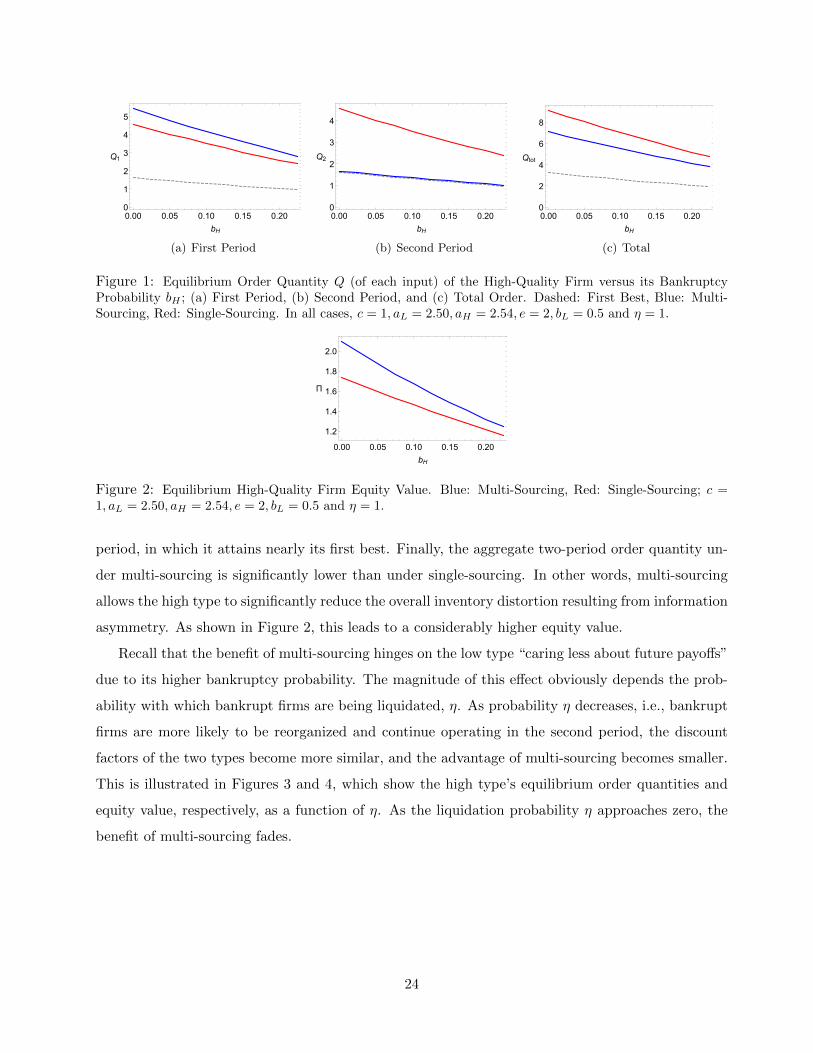
Figure 1: Equilibrium Order Quantity Q (of each input) of the High-Quality Firm versus its BankruptcyProbability bH ; (a) First Period, (b) Second Period, and (c) Total Order. Dashed: First Best, Blue: Multi-Sourcing, Red: Single-Sourcing. In all cases, c = 1, aL = 2.50, aH = 2.54, e = 2, bL = 0.5 and η = 1.

0.00 0.05 0.10 0.15 0.20

1.2

1.4

1.6

1.8

2.0

bH

Π

Figure 2: Equilibrium High-Quality Firm Equity Value. Blue: Multi-Sourcing, Red: Single-Sourcing; c =1, aL = 2.50, aH = 2.54, e = 2, bL = 0.5 and η = 1.

period, in which it attains nearly its first best. Finally, the aggregate two-period order quantity un-

der multi-sourcing is significantly lower than under single-sourcing. In other words, multi-sourcing

allows the high type to significantly reduce the overall inventory distortion resulting from information

asymmetry. As shown in Figure 2, this leads to a considerably higher equity value.

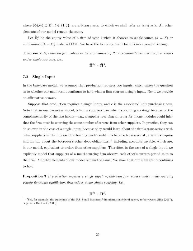
Recall that the benefit of multi-sourcing hinges on the low type “caring less about future payoffs”

due to its higher bankruptcy probability. The magnitude of this effect obviously depends the prob-

ability with which bankrupt firms are being liquidated, η. As probability η decreases, i.e., bankrupt

firms are more likely to be reorganized and continue operating in the second period, the discount

factors of the two types become more similar, and the advantage of multi-sourcing becomes smaller.

This is illustrated in Figures 3 and 4, which show the high type’s equilibrium order quantities and

equity value, respectively, as a function of η. As the liquidation probability η approaches zero, the

benefit of multi-sourcing fades.

24

0.0 0.2 0.4 0.6 0.80

1

2

3

4

η

Q1

(a) First Period

0.0 0.2 0.4 0.6 0.80.0

0.5

1.0

1.5

2.0

2.5

3.0

3.5

η

Q2

(b) Second Period

0.0 0.2 0.4 0.6 0.80

1

2

3

4

5

6

7

η

Qtot

(c) Total

Figure 3: Equilibrium Order Quantity Q (of each input) of the High-Quality Firm versus η; (a) First Period,(b) Second Period, and (c) Total Order. Dashed: First Best, Blue: Multi-Sourcing, Red: Single-Sourcing. Inall cases, c = 1, aL = 2.50, aH = 2.54, e = 2, bL = 0.5 and bH = 0.1.

0.0 0.2 0.4 0.6 0.8

1.50

1.55

1.60

1.65

η

Π

Figure 4: Equilibrium High-Quality Firm Equity Value. Blue: Multi-Sourcing, Red: Single-Sourcing; c =1, aL = 2.50, aH = 2.54, e = 2, bL = 0.5 and bH = 0.1.

7 Model Extensions

In this section, we verify the robustness of our results by considering several extensions and gener-

alizations of the model we have studied thus far.

7.1 General Belief Structure

In Section 3, we assumed that suppliers’ beliefs about their buyers’ types were threshold-based.

Under this belief structure, we showed that multi-sourcing yields a lower cost equilibrium than

single-sourcing. In this section, we confirm that this result holds true even if we allow a general

belief structure that is not necessarily threshold-based.

Consider a supplier who receives an order Q in period t. Recall that Ft is the set containing

all information observed by the supplier up to that point, which comprises prior order quantities, a

record of re-organization, or the lack thereof. We assume that the supplier forms a belief

βt(Q,Ft) =

H if Q ∈ Ht(Ft)

L o/w,

25

where Ht(Ft) ⊂ R2, t ∈ {1, 2}, are arbitrary sets, to which we shall refer as belief sets. All other

elements of our model remain the same.

Let Πki be the equity value of a firm of type i when it chooses to single-source (k = S) or

multi-source (k = M) under a LCSE. We have the following result for this more general setting:

Theorem 2 Equilibrium firm values under multi-sourcing Pareto-dominate equilibrium firm values

under single-sourcing, i.e.,

ΠM � ΠS .

7.2 Single Input

In the base-case model, we assumed that production requires two inputs, which raises the question

as to whether our main result continues to hold when a firm sources a single input. Next, we provide

an affirmative answer.

Suppose that production requires a single input, and c is the associated unit purchasing cost.

Note that in our base-case model, a firm’s suppliers can infer its sourcing strategy because of the

complementarity of the two inputs—e.g., a supplier receiving an order for phone modules could infer

that the firm must be sourcing the same number of screens from other suppliers. In practice, they can

do so even in the case of a single input, because they would learn about the firm’s transactions with

other suppliers in the process of extending trade credit—to be able to assess risk, creditors require

information about the borrower’s other debt obligations,14 including accounts payable, which are,

in our model, equivalent to orders from other suppliers. Therefore, in the case of a single input, we

explicitly model that suppliers of a multi-sourcing firm observe each other’s current-period sales to

the firm. All other elements of our model remain the same. We show that our main result continues

to hold.

Proposition 3 If production requires a single input, equilibrium firm values under multi-sourcing

Pareto-dominate equilibrium firm values under single-sourcing, i.e.,

ΠM � ΠS .

14See, for example, the guidelines of the U.S. Small Business Administration federal agency to borrowers, SBA (2017),or p.84 in Buchheit (2000).

26

7.3 Signaling by Underordering

In the base-case model, we assumed that the two types differ in two ways. First, the high type is

less likely to fail, i.e., bH < bL, and second, the high type generates a higher revenue from each

additional unit of output conditional on success, i.e., π′H (Q) > π′L (Q) . A higher probability of

success could be associated with the ability to earn a higher unit revenue when both are a result of

superior management or operations capabilities, for example.

However, it is also conceivable that the reverse could be true, e.g., when there exist two production

technologies, with the newer one being more efficient, but also more prone to failure. In this case, a

high type, i.e., a firm that faces a lower risk of failure, would earn a lower net revenue on each unit

produced conditional on success, i.e., we have bH < bL and π′H (Q) < π′L (Q) . Suppose further that

the difference in marginal revenues is such that the first-best quantity of the high type falls below

that of the low type, i.e., QfbH < Qfb

L . We can show that as long as a firm’s suppliers can observe

each other’s sales to the firm (see our discussion in Section 7.2), the high type can in this case signal

by underordering. Observability is required to ensure that the low type cannot costlessly imitate the

high type’s underordering strategy by splitting its order for a given input among multiple suppliers.

Most important, we can show that our main result continues to hold. In particular, let Πki be

the equity value of a firm of type i when it chooses to single-source (k = S) or multi-source (k = M)

under a LCSE in this setting.

Proposition 4 Equilibrium firm values under multi-sourcing Pareto-dominate equilibrium firm val-

ues under single-sourcing, i.e.,

ΠM � ΠS .

7.4 Pooling Equilibria

So far we have restricted our attention to separating equilibria (SE), leaving aside any discussion

of possible pooling outcomes. Here, we study equilibria that involve pooling and find that they are

always dominated by least-cost SE as long as the proportion of low-quality firms is not “too small.”

It is straightforward to show that any pooling outcome in the second period cannot survive the

intuitive criterion refinement of Cho and Kreps (1987). However, we cannot eliminate the possibility

that firms pool in the first period and separate in the second. Let ` be the proportion of low-

quality firms in the economy, which is also suppliers’ prior that a firm is of low type in period 1.

Intuitively, if ` is very small, the fair interest under pooling, rP (Q), is not much different from the

fair interest charged to a high type, rH(Q). In this case the high type may prefer pooling to incurring

27

the signaling cost, which is independent of `. If firms indeed pool in period 1, sourcing strategy is

irrelevant because pooling is not informative and the number of first-period suppliers has no effect

on a firm’s payoff period 2. Most important, we can show that when ` is sufficiently large, the high

type is better off separating from the outset and, therefore, has a strict preference for multi-sourcing.

We formalize the result in the next proposition.

Proposition 5 There exists ¯ ∈ (0, 1) such that if ` > ¯, the high type strictly prefers to separate

from the low type in both periods and use multi-sourcing over any other equilibrium that survives the

intuitive criterion.

7.5 Bargaining Power

Recall that under a single-sourcing strategy, when the firm transacts with the single informed supplier

in period 2, a bargaining game arises between them. Because our focus are small, risky firms dealing

with large, established suppliers, our base-case model assumed that in this situation, the supplier

has monopolistic bargaining power and extracts his maximum possible surplus. In this extension, we

relax this assumption and show that our main result holds true for any bargaining solution—including

the Nash bargaining solution, the Kalai-Smorodinsky solution, and the egalitarian solution—except

for the extreme case of the firm having monopolistic bargaining power.

In particular, let B be the firm’s extracted surplus from the aforementioned bargaining game

as a proportion of the firm’s maximum possible surplus from bargaining. Loosely speaking, B is a

measure of the firm’s bargaining power. The case of the supplier having monopolistic bargaining

power, assumed in the base-case model, corresponds to B = 0. The Nash bargaining solution, the

Kalai-Smorodinsky solution, and the egalitarian solution all correspond to values of B ∈ (0, 1). We

have the following result.

Proposition 6 For any 0 ≤ B < 1, equilibrium firm values under multi-sourcing Pareto-dominate

equilibrium firm values under single-sourcing, i.e.,

ΠM � ΠS .

Note that single-sourcing becomes equivalent to multi-sourcing if B = 1, i.e., when the firm has

monopolistic bargaining power. However, this case is incompatible with our intention of studying

small, risky buyers sourcing from large, well-established suppliers.

28

8 Conclusion

Existing theories of supplier diversification are based on the premise that the bulk of the risk in

trade relationships originates from suppliers. In this context, diversification is put forth as a means

to hedge against supply-side risks. This view is well suited for situations in which large buyers

source from smaller, riskier, or less well-established suppliers and has roots in the way traditional

supply chains used to operate. But this setting is inadequate to describe sourcing strategies when

the premise is reversed, for instance, when risky firms, such as SMEs or startups, are dealing with

well established suppliers. What’s more, this alternative setting is increasingly relevant in modern

modular supply chains, in which firms operate both as buyers and suppliers, and can be exposed to

risks on either side.

This paper argues that a firm’s own risk can drive its sourcing strategy. Inspired by some of the

difficulties that startup firms often encounter in practice, we start from the premise that a firm’s risk

can represent an obstacle in its attempt to access a competitive supply market. In such situations,

the firm has the incentive to make an up-front investment (i.e., take costly actions) to convince

suppliers of its quality, so as to unlock fair access to the market. So doing, however, could leave the

firm exposed to supplier opportunism, which in our model, takes the form of informational holdup.

Supplier diversification can then be put forth as a means to alleviate this opportunism. By arguing

that a firm’s own riskiness, not just the riskiness of its suppliers, should be an important driver of its

sourcing strategy, our work identifies a new strategic dimension that young firms, and in particular

startups, may want to consider when contemplating their long-term sourcing strategy.

There are some immediate extensions that would make our model more realistic but would not

affect qualitative insights. For example, one may reflect the increased cost of complexity when dealing

with multiple suppliers. Clearly, if this cost is high enough, it will eventually overcome the advantage

of multi-sourcing identified here. More involved extensions that may provide potentially interesting

insights could consider supplier heterogeneity (cost, quality, risk), different competitive structures of

the supplier industry (e.g., oligopoly), alternative signaling mechanisms, and different types of buyer

risk or supplier opportunism. Finally, there could be other channels through which buyer risk could

motivate supplier diversification, which could be explored in future research.

References

Alos-Ferrer, C, and J Prat. 2012. “Job market signaling and employer learning.” Journal of Economic

Theory, 147: 1787–1817.

29

Ang, E, DA Iancu, and R Swinney. 2016. “Disruption Risk and Optimal Sourcing in Multitier Supply

Networks.” Management Science, Articles in Advance.

Babich, V, AN Burnetas, and PH Ritchken. 2007. “Competition and diversification effects in supply

chains with supplier default risk.” Manufacturing & Service Operations Management, 9(2): 123–146.

Babich, V, and CS Tang. 2012. “Managing opportunistic supplier product adulteration: Deferred payments,

inspection, and combined mechanisms.” Manufacturing & Service Operations Management, 14(2): 301–

314.

Babich, V, G Aydin, P-Y Brunet, J Keppo, and R Saigal. 2010. Risk, financing, and the optimal num-

ber of suppliers. H. Gurnani, A. Mehrotra, S. Ray, eds. Managing Supply Disruptions. London:Springer-

Verlag.

Baldwin, Carliss Young, and Kim B Clark. 2000. Design rules: The power of modularity. Vol. 1, MIT

press.

Bimpikis, K, D Fearing, and A Tahbaz-Salehi. 2017. “Multi-Sourcing and Miscoordination in Supply

Chain Networks.”

Bimpikis, K, O Candogan, and S Ehsani. 2014. “Supply Disruptions and Optimal Network Structures.”

Buchheit, LC. 2000. How to negotiate eurocurrency loan agreements. Vol. 2, Euromoney Institutional In-

vestor.

Burkart, M, and T Ellingsen. 2004. “In-kind finance: A theory of trade credit.” American Economic

Review, 94(3): 569–590.

Cheng, J. 2016. “Smartphone Makers Look Beyond the Device.” https: // www. wsj. com/ articles/

smartphone-makers-look-beyond-the-device-1456434361 .

Chod, J. 2016. “Inventory, Risk Shifting, and Trade Credit.” Management Science.

Chod, J, N Trichakis, and G Tsoukalas. 2017. “A Signaling Theory of In-Kind Finance.” Working Paper.

Cho, IK, and M Kreps. 1987. “Signaling games and stable equilibria.” Quarterly Journal of Economics,

102(2): 179–221.

Dada, M, and NC Petruzzi. 2007. “A newsvendors procurement problem when suppliers are unreliable.”

Manufacturing & Service Operations Management, 9(1): 9–32.

Dong, L, and B Tomlin. 2012. “Managing disruption risk: The interplay between operations and insurance.”

Management Science, 58(10): 1898–1915.

Federgruen, A, and N Yang. 2007. “Optimal supply diversification under general supply risks.” Operations

Research, 57(6): 1451–1468.

Feng, Tianjun, and Fuqiang Zhang. 2014. “The impact of modular assembly on supply chain efficiency.”

Production and Operations Management, 23(11): 1985–2001.

Fisman, R, and M Raturi. 2004. “Does competition encourage credit provision? Evidence from African

Trade Credit Relationships.” Review of Economic Studies, 86(1): 345–352.

30

Giannetti, M, M Burkart, and T Ellingsen. 2011. “What you sell is what you lend? Explaining trade

credit contracts.” Review of Financial Studies, 24(4): 1261–1298.

Hale, G, and JAC Santos. 2009. “Do banks price their informational monopoly?” Journal of Financial

Economics, 93: 185–206.

Hasija, Sameer, Edieal J Pinker, and Robert A Shumsky. 2008. “Call center outsourcing contracts

under information asymmetry.” Management Science, 54(4): 793–807.

Hermalin, BE. 2010. “Holdup: Implications for Investment and Organization.” California Management

Review, 52(2): 132–137.

Humrick, M. 2016. “The Meizu PRO 6 Review.” http: // www. anandtech. com/ show/ 10545/

the-meizu-pro-6-review .

Jain, N, K Girotra, and S Netessine. 2015. “Recovering from Supply Interruptions: The Role of Sourcing

Strategy.” INSEAD Working Paper No. 2016/58/TOM.

Kaya, Ayca. 2009. “Repeated Signaling Games.” Games and Economic Behavior, 66: 841–854.

Kouvelis, P, and SY Tang. 2011. “Supplier Diversification Strategies in the Presence of Yield Uncertainty

and Buyer Competition.” Manufacturing & Service Operations Management, 13(13): 1523–4614.

Kouvelis, P, and W Zhao. 2012. “Financing the newsvendor: Suppliers vs. Bank, and the Structure of

Optimal trade credit contracts.” Operations Research, 60(94): 569–590.

Kreps, DM, and R Wilson. 1982. “Reputation and Imperfect Information.” Journal of Economic Theory,

27: 253–279.

Lai, G, and W Xiao. 2016. “Inventory Decisions and Signals of Demand Uncertainty to Investors.” Working

Paper.

Lai, G, W Xiao, and J Yang. 2012. “Supply chain performance under market valuation: An operational

approach to restore efficiency.” Management Science, 57(2): 332–346.

Li, C, and LR Debo. 2009. “Second Sourcing vs. Sole Sourcing with Capacity Investment and Asymmetric

Information.” Manufacturing & Service Operations Management, 11(3).

Li, Z, SM Gilbert, and G Lai. 2014. “Supplier Encroachment Under Asymmetric Information.” Manage-

ment Science, 60(2): 449–462.

Luo, W, and K Shang. 2013. “Managing inventory for entrepreneurial firms with trade credit and payment

defaults.” Working Paper.

Pei, PP-E, D Simchi-Levi, and TI Tunca. 2011. “Sourcing Flexibility, Spot Trading, and Procurement

Contract Structure.” Operations Research, 59(3): 578–601.

Petersen, MA, and RG Rajan. 1997. “Trade credit: Theories and Evidence.” Review of Financial Studies,

10(3): 661–691.

Rui, H, and G Lai. 2015. “Sourcing with Deferred Payment and Inspection under Supplier Product Adul-

teration Risk.” Production and Operations Management, 24(6): 934–946.

31

SBA. 2017. “Loans & Grants. United States Small Business Administration (SBA).” https: // www. sba.

gov/ loans-grants/ get-ready-apply/ gather-info-youll-need .

Schenone, C. 2010. “Lending relationships and information rents: do banks exploit their informational

advantages?” Review of Financial Studies, 23(3): 1149–1199.

Schmidt, W, V Gaur, R Lai, and A Raman. 2015. “Signaling to partially informed investors in the

newsvendor model.” Prod. Oper. Manag., 24(3): 383–401.

Spence, M. 1973. “Job Market Signaling.” Quarterly Journal of Economics, 87(3): 355–374.

Stuckey, J, and D White. 1993. “When and When Not to Vertically Integrate.” McKinsey Quarterly, , (3).

Taylor, TA, and EL Plambeck. 2007. “Supply Chain Relationships and Contracts: The Impact of Repeated

Interaction on Capacity Investment and Procurement.” Management Science, 53(10): 1577–1593.

Tomlin, B. 2006. “On the value of mitigation and contingency strategies for managing supply chain disruption

risks.” Management Science, 52(5): 639–657.

Tomlin, B. 2009a. “The impact of supply learning when suppliers are unreliable.” Manufacturing & Service

Operations Management, 11(2): 192–209.

Tomlin, B, and Wang. 2010. Operational strategies for managing supply chain disruption risk. P. Kouvelis,

O. Boyabatli, L. Dong, R. Li, eds. New York:John Wiley & Sons.

Tomlin, Brian. 2009b. “Disruption-management strategies for short life-cycle products.” Naval Research

Logistics (NRL), 56(4): 318–347.

Tomlin, Brian, and Yimin Wang. 2005. “On the value of mix flexibility and dual sourcing in unreliable

newsvendor networks.” Manufacturing & Service Operations Management, 7(1): 37–57.

Tunca, TI, and Q Wu. 2009. “Multiple Sourcing and Procurement Process Selection with Bidding Events.”

Management Science, 55(5): 763–780.

Wang, Yimin, Wendell Gilland, and Brian Tomlin. 2011. “Regulatory trade risk and supply chain

strategy.” Production and Operations Management, 20(4): 522–540.

Wang, Y, W Gilland, and B Tomlin. 2010. “Mitigating Supply Risk: Dual Sourcing or Process Improve-

ment?” Manufacturing & Service Operations Management, 12(3): 489–510.

Williamson, O. 1971. “The Vertical Integration of Production: Market Failure Considerations.” American

Economic Review, 62(2).

Wu, Xiaole, and Fuqiang Zhang. 2014. “Home or overseas? An analysis of sourcing strategies under

competition.” Management Science, 60(5): 1223–1240.

Yang, Z, G Aydin, V Babich, and Beil DR. 2012. “Using a Dual-Sourcing Option in the Presence of

Asymmetric Information About Supplier Reliability: Competition vs. Diversification.” Manufacturing &

Service Operations Management, 14(2): 202–217.

Yoshida, J. 2014. “Exclusive: Xiaomi Challenged. Xiaomis rollercoaster ride continues.” http: // www.

eetimes. com/ document. asp? doc_ id= 1321490& page_ number= 1 .

32

Yu, H. 2014. “How Xiaomi wooed the best suppliers.” https: // www. ft. com/ content/

6a675fe2-a9c6-11e3-adab-00144feab7de .

Zhao, X, L Xue, and F Zhang. 2014. “Outsourcing Competition and Information Sharing with Asymmet-

rically Informed Suppliers.” Production and Operations Management, 23(10): 17061718.

33

A Proofs

Proof of Lemma 1: We first prove that the expected payoffs of the two types satisfy the single

crossing property, i.e.,

vLL (Q1) ≤ vLH (Q2)⇒ vHL (Q1) < vHH (Q2) (21)

for any Q2 > Q1. Suppose Q2 > Q1. Using (7), statement (21) can be written as

cQ2

1− bH− cQ1

1− bL≤ πL (Q2)− πL (Q1)⇒ cQ2

1− bH− cQ1

1− bL< πH (Q2)− πH (Q1) . (22)

Thus, to prove (22), it is enough to prove

πL (Q2)− πL (Q1) < πH (Q2)− πH (Q1)⇔ (23)∫ Q2

Q1

π′L (Q) dQ <

∫ Q2

Q1

π′H (Q) dQ, (24)

which follows from the assumption π′H (Q) > π′L (Q) .

Next, we prove the desired result separately for sourcing from a single supplier and for sourcing

from two suppliers.

Sourcing from a single supplier. Because vLH (Q) is continuous and concave, and vLH (0) = 0,

vLH

(Qfb

L

)> vLL

(Qfb

L

)and lim

Q→∞vLH (Q) = −∞, eq. (10) has two roots, the larger of which satisfies

q > QfbL . To exclude trivial equilibria in which the high type can separate while ordering its first-best

quantity, we assume q > QfbH . Next, we show that, independent of whether the firm underwent

re-organization, q satisfies conditions (8) and (9), starting with the latter. Because QfbL < q, the LHS

of (9) is vLL

(Qfb

L

). Because vLH (Q) is decreasing for Q ≥ q, the RHS of (9) is equal to vLH (q) ,

and condition (9) is satisfied as equality.

Next, we prove that q satisfies condition (8) by showing that vHL (Q) ≤ vHH (q) for any Q < q.

Given (21), it is enough to show that vLL (Q) ≤ vLH (q) for any Q < q. This follows from (10)

and the definition of QfbL . Thus, we proved that q satisfies both (8) and (9). This, the fact that

QfbL < Qfb

H < q, and the concavity of vHH(Q) together imply that order quantities[Qfb

L , q]

with the

belief threshold q are a SE.

To prove that this is a LCSE, we need to show that there is no SE in which the high type

is better off. Because vHH(Q) is decreasing for Q > q > QfbH , such an equilibrium would have

to have a threshold belief q < q. However, a threshold q < q cannot be a SE belief because if it

were, the low type could order q − ε, in which case it would be perceived as the high type and

34

vLH(q − ε) > vLH (q) = vLL

(Qfb

L

).

Sourcing from two suppliers. We first show, by contradiction, that a strategy profile where either

type orders Q1 6= Q2 cannot be a SE. Suppose the high type chooses Q1 6= Q2 at a SE. At any SE,

the high type needs to choose Q1 ≥ q and Q2 ≥ q. Because the inputs are perfect complements, the

high type can always improve its payoff by simply reducing the larger of the two quantities. Thus,

Q1 6= Q2 cannot be the high type’s SE quantities, and similarly for the low type.

When a firm chooses Q1 = Q2, its payoff is the same as under single-sourcing. Thus, to prove

that the order quantities and belief threshold characterized in Lemma 1 are a unique LCSE under

multi-sourcing, it is enough to show that neither type can improve its payoff by deviating from this

strategy profile to some[Q1, Q2

]such that Q1 6= Q2. This follows again from the perfect comple-

mentarity of the two inputs.�

Proof of Lemma 2: We consider the payoffs of the two types one by one.

High type. If the high type orders Q < s2 from the informed supplier, it is considered low and its

payoff is necessarily below its reservation payoff.

If the high type orders Q ≥ s2 from the informed supplier, it is considered high, but the supplier

charges interest rM (Q) that extracts any value above the firm’s reservation payoff (if there is any).

Thus, in either case, the high type cannot earn more than its reservation payoff by ordering from

the informed supplier. Therefore, its second-period payoff is always equal to its reservation payoff

vHH (q) .

Low Type. To derive the low type’s payoff, we consider two cases.

Case 1: s2 < q. If the low type orders Q < s2 from the informed supplier, it is recognized as

low type and its payoff cannot exceed vLL

(Qfb

L

). Now suppose that the low type orders Q ≥ s2

from the informed supplier. It is considered a high type and charged the monopolistic interest

rM (Q) . Because the firm chooses the optimal order quantity, its payoff is maxQ≥s2

vL ([Q,Q] , rM (Q)) . To

prove that maxQ≥s2

vL ([Q,Q] , rM (Q)) > vLL

(Qfb

L

), we show that there exists a feasible order quantity

Q = q − ε ≥ s2 such that vL ([q − ε, q − ε] , rM (q − ε)) > vLL

(Qfb

L

). Because vL ([Q,Q] , rM (Q)) is

continuous, it is enough to show that (i) vL ([q, q] , rM (q)) = vLL

(Qfb

L

)and (ii) vL ([Q,Q] , rM (Q)) is

strictly decreasing in Q ∈ [q−ε, q). To show (i), note that rM (q) = rH (q) and so vL ([q, q] , rM (q)) =

vLH (q) = vLL

(Qfb

L

). To show (ii), note that for any Q ∈ [q − ε, q), we have vH ([Q,Q] , rH (Q)) >

35

vHH (q) , and so rM (Q) is given by (11). Thus

rM (Q) = πH (Q)− cQ− πH (q) +cq

1− bHand, thus, (25)

vL ([Q,Q] , rM (Q)) = (1− bL)

(πL (Q)− πH (Q) + πH (q)− cq

1− bH

), and (26)

d

dQvL ([Q,Q] , rM (Q)) = (1− bL)

(π′L (Q)− π′H (Q)

)< 0. (27)

Thus, the low type orders Q ≥ s2 from the informed supplier and earns maxQ≥s2

vL ([Q,Q] , rM (Q)) >

vLL

(Qfb

L

).

Case 2: s2 = q. If the belief threshold of the informed supplier is as high as the belief threshold

of uninformed suppliers, the low type cannot earn a payoff above its reservation payoff vLL

(Qfb

L

).�

Proof of Lemma 3: The result follows directly from the discussion preceding Lemma 3. �

Proof of Proposition 1: To establish the result, we consider two cases.

Case 1: s2 = q. Using Lemma 2, the firms’ second-period payoffs become independent of their first-

period actions, the equilibrium conditions (13) and (14) simplify into (8) and (9), and the first period

is thus equivalent to a single-period game in the absence of informed suppliers. Invoking Lemma

1, the only first-period order quantities and belief threshold that can be a LCSE are(Qfb

L , q)

and

s1 = q, and they result in first-period payoffs vHH (q) and vLL

(Qfb

L

)for the two types, respectively.

In the second period, the high type orders q units from either the informed supplier or an uninformed

supplier, in each case earning vHH (q). The low type orders its first best and earns vLL

(Qfb

L

).

Case 2: s2 < q. It follows from Lemma 2 and condition (14) that maxQ<s1

vLL (Q) > maxQ≥s1

vLH (Q) .

Invoking (10), this inequality implies s1 > q, which in turn implies that the high type’ first-period

payoff is below vHH (q) . Because the high type’s second-period payoff is always vHH (q) and the

low type’s payoff in each period is vLL

(Qfb

L

), any SE with s2 < q is Pareto-dominated by the SE

where s2 = q.

Thus, the SE where s2 = q is the unique LCSE. �

Proof of Proposition 2: We first prove the existence of a SE by verifying that the low type

ordering QfbL and the high type ordering q in each period, and belief thresholds m1 = m2 = q is a SE.

If we substitute q for both m1 and m2, the equilibrium conditions (16) and (17) simplify into (8) and

(9), which are satisfied by the definition of q. Under this belief structure, the two-period problem

36

decouples into two single-period problems, and we know from Lemma 1 that the order quantities,

QfbL and q, and belief threshold q are indeed a SE.

Next, we characterize a LCSE. Suppose m1 ≤ QfbH . Because Qfb

H < q, this implies m1 < q. This

together with m2 ≤ q means that (17) cannot be satisfied. Hence, we must have m1 > QfbH , and

conditions (16) and (17) simplify into

maxQ

vHL (Q) + (1− ηbH) vHH (q) ≤ vHH (m1) + (1− ηbH) maxQ≥m2

vHH (Q) and (28)

vLL

(Qfb

L

)+ (1− ηbL) vLL

(Qfb

L

)≥ vLH (m1) + (1− ηbL) max

Q≥m2

vLH (Q) . (29)

Now suppose m2 < QfbH . This cannot correspond to a LCSE because any SE under this belief

structure is strictly Pareto-dominated by the same SE with m2 being replaced by QfbH . (This is

because replacing m2 with QfbH will not change the second-period payoff of the high type, but it

will strictly reduce the second-period payoff of the low type that signals in the first period. This

will in turn decrease the low type’s willingness to signal in the first period captured by m1. Because

m1 > QfbH , reducing m1 will reduce the high type’s first-period signaling cost.) Thus, at any LCSE

we must have m2 ≥ QfbH .

The fact that m2 ≥ QfbH implies that both vHH (Q) and vLH (Q) are decreasing for Q ≥ m2 and,

therefore, conditions (28) and (29) simplify into

maxQ

vHL (Q) + (1− ηbH) vHH (q) ≤ vHH (m1) + (1− ηbH) vHH (m2) and (30)

vLL

(Qfb

L

)+ (1− ηbL) vLL

(Qfb

L

)≥ vLH (m1) + (1− ηbL) vLH (m2) . (31)

The LCSE belief structure is one that maximizes the high type’s total equilibrium payoff, which is

the RHS of (30), while ensuring that the low type does not imitate, i.e., condition (31) holds.

Finally, suppose condition (31) is satisfied as a strict inequality for some SE belief structure

(m1,m2). If this is the case, there must be some (m1 − ε,m2) that also satisfies condition (31), but

results in a strictly larger RHS of (30). Thus, (m1,m2) cannot be a LCSE. Therefore, at any LCSE

condition (31) must be satisfied as an equality, and the desired result follows. �

Proof of Theorem 1: Note that m1 = m2 = q satisfies conditions (16) and (17), i.e., m1 = m2 = q

is a SE under multi-sourcing. Furthermore, firm equity values at this particular multi-sourcing SE

are the same as those under the single-sourcing LCSE.

Next, we show that under multi-sourcing, this particular SE is not a LCSE, i.e., we show that

37

m1 = m2 = q, which is clearly a feasible solution of problem (18), is not its optimal solution. To do

that, we reformulate (18) as

m1 ∈ arg maxm1≥q

[vHH (m1) + (1− ηbH) vHH (m2 (m1))] , (32)

where function m2 (m1) is given implicitly by the larger root of

(2− ηbL) vLL

(Qfb

L

)= vLH (m1) + (1− ηbL) vLH (m2) . (33)

Taking the total derivative of the objective function in (32) w.r.t. m1 yields

v′HH (m1)−(1− ηbH) v′LH (m1)

(1− ηbL) v′LH (m2)v′HH (m2) . (34)

Evaluating this derivative at m1 = q gives

v′HH (q)

(1− (1− ηbH)

(1− ηbL)

)> 0. (35)

Thus, m1 = q cannot be the optimal solution of (32), i.e., m1 = m2 = q cannot be the optimal

solution of (18) even though it is clearly feasible. Therefore, the optimal solution of (18) must

provide a larger value of the objective than m1 = m2 = q does. This means that under multi-

sourcing, the LCSE must result in a larger payoff for the high type than the SE where m1 = m2 = q,

which gives the same payoffs as the LCSE under single-sourcing.

Finally, note that according to (18), m2 = q implies m1 = q. Since this is not a LCSE under

multi-sourcing, a LCSE must have m2 < q, which, according to (18), requires m1 > q. This, together

with Proposition 1, implies that the LCSE thresholds satisfy m1 > s1 = q = s2 > m2. �

Proof of Theorem 2. To introduce some notation first, we denote the information available to

a supplier at the begining of the second period with F2 = (Q, I), where Q and I are interpreted as

follows. If the supplier transacted with the firm before, Q is the prior order it received; otherwise

we write Q = ∅. The signal I equals R or NR, depending on whether the firm went through re-

organization or not. We can then write the second-period belief setH2(F2) also asH2(Q, I). Because

no information is available at the beginning of the first period, we write the first-period belief set

simply as H1.

Consider some belief sets Ht(Ft) for t ∈ {1, 2} and all possible Ft’s, that are consistent with a

38

separating equilibrium. The existence of such a collection of sets is guaranteed by our analysis in

§5 that identified interval sets of the form [h,∞), which formed a threshold-type SE belief system.

Because under a SE the low type orders its first-best quantity and no order below that quantity is

credible in either period, we have

Ht(Ft) ⊂ (QfbL ,∞)× (Qfb

L ,∞), ∀Ft, t ∈ {1, 2}. (36)

We analyze the single-sourcing strategy first. Consider a firm in period 2. There are two cases:

the firm has access to either one informed supplier or none. Let vi(1,F2) be the second-period payoff

of type i if it has access to 1 informed supplier that has observed F2 = (Q, I). Let also vi(0,F2)

be the second-period payoff of type i if it has access only to uniformed suppliers that have observed

F2 = (∅, I). (We are assuming without a loss that the firm will never source from a supplier to

which it signaled low in period 1.) These payoffs are generalizations of the payoffs we derived in

Lemmata 1-3. We can characterize these second-period payoffs as follows:

• When having access to no informed suppliers, the firm transacts with a new supplier and

F2 = (∅, I). The firm can then can signal high or low, and if its true type is i, its payoff is

given by

vi(0, (∅, I)) = max

{max

[Q;Q]∈H2(∅,I)viH(Q), max

[Q;Q]/∈H2(∅,I)viL(Q),

}, i ∈ {L,H}, (37)

where vij(·) was defined in (7).

• When having access to one informed supplier, using similar arguments as in the proof of

Lemma 2, it can be readily seen that a firm of high type is “held up” and, therefore,

vH(1, (Q, I)) = vH(0, (∅, I)), ∀(Q, I). (38)

A firm of low type has always the option of transacting with an uninformed supplier and, thus,

vL(1, (Q, I)) ≥ vL(0, (∅, I)), ∀(Q, I). (39)

Consider now the full two-period game. At a SE, the low type signals its true type in both

periods and obtains its first-best payoff, vLL

(Qfb

L

). Therefore, in the second period it has no access

39

to informed suppliers. Combining these two facts and (37) we get that

vLL

(Qfb

L

)= vL(0, (∅, I)) ≥ max

[Q;Q]∈H2(∅,I)vLH(Q), ∀I. (40)

Consider now the critical quantity q we introduced in Lemma 1. As we showed in the proof of that

Lemma, we have that vLH(Q) > vLL

(Qfb

L

)for all Qfb

L < Q < q. Therefore, we conclude that

H2(∅, I) ⊂ [q,∞)× [q,∞), ∀I. (41)

To derive the SE conditions for the first period, let’s consider first the off-equilibrium path in

which the low type orders a quantity Q ∈ H1 and imitates the high type. Its expected payoff is then

given by

vLH(Q) + E [vL(1, ([Q;Q], I) 1C ] ,

where 1C is the indicator of the firm continuing into the second period, and the expectation is taken

over bankruptcy and re-organization. Under a SE, the low type shall be better off revealing its true

type rather than imitating the high type. That is,

max[Q;Q]∈H1

{vLH(Q) + E [vL(1, ([Q;Q], I) 1C ]

}≤ (2− ηbL)vLL(Qfb

L ), (42)

where the right-hand side of the inequality is the low-type’s expected payoff under a SE (cf. Propo-

sition 1).

Suppose now that there exists a Q = [Q;Q] ∈ H1 such that vLH(Q)> vLL(Qfb

L ). That leads to

the following contradiction:

max[Q;Q]∈H1

{vLH(Q) + E [vL(1, ([Q;Q], I) 1C ]

}≥ vLH(Q) + E

[vL(1, (Q, I) 1C

]≥ vLH(Q) + E [vL(0, (∅, I) 1C ]

= vLH(Q) + E[vLL(Qfb

L ) 1C

]> vLL(Qfb

L ) + (1− ηbL)vLL(QfbL )

= (2− ηbL)vLL(QfbL ),

where the second inequality follows from (39), the first equality from the equality in (40), and the

final inequality from evaluating the continuation probability and our assumption above. Given that

40

vLH (Q) ≤ vLL(QfbL ) for all [Q;Q] ∈ H1, we conclude that

H1 ⊂ [q,∞)× [q,∞). (43)

We now switch our attention to the high type. In the second period, as we remarked above, the

high type is “held up” and, therefore, we can assume without a loss that under a SE it transacts

with an uninformed supplier. Consequently, we get

vH(0, (∅, I)) = max[Q;Q]∈H2(∅,I)

vHH(Q) ≤ vHH(q), ∀I, (44)

where the equality follows from (37) and the fact that the high type signals its type under a SE,

and the inequality from (41) and the fact that vHH is decreasing in [q,∞). Suppose that in the first

period under a SE, the high type orders Q = [Q; Q] ∈ H1. Then, its payoff is given by

vHH(Q) + E[vH(1, (Q, I) 1C

]= vHH(Q) + E [vH(0, (∅, I) 1C ]

≤ vHH(Q) + E [vHH(q) 1C ]

= vHH(Q) + (1− ηbH)vHH(q)

≤ vHH(q) + (1− ηbH)vHH(q) = (2− ηbH)vHH(q),

where the first equality follows from (38), the first inequality from (44), and the second inequality

from (43) and the fact that vHH is decreasing in [q,∞). Given that the belief system and Q were

arbitrarily chosen so as to only satisfy necessary conditions for a SE, we get that

ΠSH ≤ (2− ηbH)vHH(q).

To complete the proof, note that the LCSE equity value of a multi-sourcing high type under this

more general game, ΠMH , is greater than or equal to the LCSE equity value of a multi-sourcing high

type under the original game, ΠMH . Thus,

ΠMH ≥ ΠM

H > (2− ηbH)vHH(q) ≥ ΠSH ,

where the strict inequality follows from Theorem 1.

Proof of Proposition 3: We prove the result by showing that our base-case two-input model and

41

a model, in which production requires a single input with a unit cost c = c1 + c2 are equivalent, i.e.,

they result in the same payoffs for both types as functions of production quantity Q and thresholds

q, s1, s2,m1,m2. Under single-sourcing, the number of inputs is clearly irrelevant as one can think

of the two inputs as a single input with cost c = c1 + c2.

Next, consider multi-sourcing in either period. For any given production quantity Q, value of

type i is vi (Q, r) := Emax {πi (Q)− cQ− r (Q) , 0} in both two-input and single-input scenarios.

Thus, it is enough to show that for any given production quantity Q and belief threshold t, each

type is charged the same total interest r (Q) in both scenarios. We characterize this interest in the

two scenarios next.

Total interest in the base-case two-input scenario. Recall that a multi-sourcing firm orders

Q units of one input from one supplier and Q units of the other input from another supplier. If

supplier of input i believes the firm to be of type j, it charges fair interest rij(Q) that satisfies the

break-even condition

(1− bj)(ciQ+ rij (Q)

)= ciQ,

where RHS is the input cost and the LHS is the expected payment. Thus, this interest can be

written explicitly as rij (Q) =bj

1−bj ciQ. Because each supplier forms its belief by comparing the order

quantity Q and threshold t, the total interest faced by the firm is

r (Q) =

r1H (Q) + r2

H (Q) = bH1−bH cQ if Q ≥ t,

r1L (Q) + r2

L (Q) = bL1−bL cQ o/w

. (45)

Total interest in the single-input scenario. Suppose that a firm splits the total input order Q

between two suppliers in proportions γ1 ∈ (0, 1) and γ2 = 1 − γ1. If supplier i believes the firm to

be of type j, it charges fair interest that satisfies the break-even condition

(1− bj)(cγiQ+ rij (γiQ)

)= cγiQ,

and is thus equal to rij (γiQ) =bj

1−bj cγiQ. Because each of the two suppliers forms its belief by

comparing the total order quantity Q and threshold t, the firm faces total interest

r (Q) =

r1H (γ1Q) + r2

H (γ2Q) = bH1−bH cQ if Q ≥ t,

r1L (γ1Q) + r2

L (γ2Q) = bL1−bL cQ o/w

. (46)

Because the two scenarios lead to the same trade credit interests and, thus, the same firm values,

42

they also result in the same equilibrium payoffs. Therefore, Theorem 1 continues to hold in the

single-input scenario. �

Proof of Proposition 4: Suppose without loss of generality that production requires two inputs

and suppliers’ belief structure is

β :=

H if Q ≤ t,

L o/w,j ∈ {1, 2}, (47)

for some endogenous threshold t. We first consider the second period.

(a) No Access to Informed Suppliers. This situation is equivalent to a single-period game,

so there is no difference between single- and multi-sourcing, We assume for simplicity that firms

source from a single supplier. The only difference from our base-case is that the conditions for a

separating equilibrium belief threshold q change as follows:

maxQ>q

vHL (Q) ≤ maxQ≤q

vHH (Q) and (48)

maxQ>q

vLL (Q) ≥ maxQ≤q

vLH (Q) . (49)

Next, we prove that analogously to Lemma 1, the low type orders its first best, QfbL , of each input and

earns vLL(QfbL ), whereas the high type reduces its order to q units of each input and earns vHH(q),

where q is the smaller of the two roots of

vLH (q) = vLL

(Qfb

L

). (50)

We first show that the expected payoffs of the two types satisfy the following property, i.e.,

vLL (Q2) ≤ vLH (Q1)⇒ vHL (Q2) < vHH (Q1) (51)

for any Q2 > Q1. Suppose Q2 > Q1. Using (7), statement (51) can be written as

cQ1

1− bH− cQ2

1− bL≤ πL (Q1)− πL (Q2)⇒ cQ1

1− bH− cQ2

1− bL< πH (Q1)− πH (Q2) . (52)

43

Thus, to prove (52), it is enough to prove

πL (Q1)− πL (Q2) < πH (Q1)− πH (Q2)⇔ (53)

πL (Q2)− πL (Q1) > πH (Q2)− πH (Q1)⇔ (54)∫ Q2

Q1

π′L (Q) dQ >

∫ Q2

Q1

π′H (Q) dQ, (55)

which follows from the assumption π′L (Q) > π′H (Q) .

Because vLH (Q) is continuous and concave, and vLH (0) = 0, vLH

(Qfb

L

)> vLL

(Qfb

L

)and

limQ→∞

vLH (Q) = −∞, eq. (50) has two roots, the smaller of which satisfies q < QfbL . To exclude

trivial equilibria in which the high type can separate while ordering its first-best quantity, we assume

q < QfbH . Next, we show that q satisfies conditions (48) and (49), starting with the latter. Because

QfbL > q, the LHS of (49) is vLL

(Qfb

L

). Because vLH (Q) is increasing for Q ≤ q, the RHS of (49) is

equal to vLH (q) , and condition (49) is satisfied as equality.

Next, we prove that q satisfies condition (48) by showing that vHL (Q) ≤ vHH (q) for any Q > q.

Given (51), it is enough to show that vLL (Q) ≤ vLH (q) for any Q > q. This follows from (50)

and the definition of QfbL . Thus, we proved that q satisfies both (48) and (49). This, the fact that

q < min{Qfb

L , QfbH

}, and the concavity of vHH(Q) together imply that order quantities

[Qfb

L , q]

with the belief threshold q are a SE.

To prove that this is a LCSE, we need to show that there is no SE, in which the high type

is better off. Because vHH(Q) is increasing for Q < q < QfbH , such an equilibrium would have

to have a threshold belief q > q. However, a threshold q > q cannot be a SE belief because if it

were, the low type could order q + ε, in which case it would be perceived as the high type and

vLH(q + ε) > vLH (q) = vLL

(Qfb

L

).

(b) Access to One Informed Supplier. Analogously to the base case, we assume without

any loss of generality that s2 ≥ q. We prove that analogously to Lemma 2, the high type earns its

reservation payoff vHH (q), whereas the low type earns a payoff

vLH =

maxQ≤s2

vL ([Q,Q] , rM (Q)) > vLL

(Qfb

L

)if s2 > q,

vLL

(Qfb

L

)o/w.

Consider the high type first. If the high type orders Q > s2 from the informed supplier, it is

considered low and its payoff is necessarily below its reservation payoff. If the high type orders

Q ≤ s2 from the informed supplier, it is considered high, but the supplier charges interest rM (Q)

44

that extracts any potential value above the firm’s reservation payoff. Thus, the high type cannot earn

more than its reservation payoff by ordering from the informed supplier. Therefore, its second-period

payoff is always equal to its reservation payoff vHH (q) .

To derive the low type’s payoff, we consider two cases.

Case 1: s2 > q. If the low type orders Q > s2 from the informed supplier, it is recognized as

low type and its payoff cannot exceed vLL

(Qfb

L

). Now suppose that the low type orders Q ≤ s2

from the informed supplier. It is considered a high type and charged the monopolistic interest

rM (Q) . Because the firm chooses the optimal order quantity, its payoff is maxQ≤s2

vL ([Q,Q] , rM (Q)) . To

prove that maxQ≤s2

vL ([Q,Q] , rM (Q)) > vLL

(Qfb

L

), we show that there exists a feasible order quantity

Q = q + ε ≤ s2 such that vL ([q + ε, q + ε] , rM (q + ε)) > vLL

(Qfb

L

). Because vL ([Q,Q] , rM (Q)) is

continuous, it is enough to show that (i) vL ([q, q] , rM (q)) = vLL

(Qfb

L

)and (ii) vL ([Q,Q] , rM (Q)) is

strictly increasing in Q ∈ (q, q+ε]. To show (i), note that rM (q) = rH (q) and so vL ([q, q] , rM (q)) =

vLH (q) = vLL

(Qfb

L

). To show (ii), note that for any Q ∈ (q, q + ε], we have vH ([Q,Q] , rH (Q)) >

vHH (q) , and so rM (Q) is given by (11). Thus

rM (Q) = πH (Q)− cQ− πH (q) +cq

1− bHand, thus, (56)

vL ([Q,Q] , rM (Q)) = (1− bL)

(πL (Q)− πH (Q) + πH (q)− cq

1− bH

), and (57)

d

dQvL ([Q,Q] , rM (Q)) = (1− bL)

(π′L (Q)− π′H (Q)

)> 0. (58)

Thus, the low type orders Q ≤ s2 from the informed supplier and earns maxQ≤s2

vL ([Q,Q] , rM (Q)) >

vLL

(Qfb

L

).

Case 2: s2 = q. If the belief threshold of the informed supplier is as low as the belief threshold of

uninformed suppliers, the low type cannot earn a payoff above its reservation payoff vLL

(Qfb

L

).

(c) Access to Two Informed Suppliers. Analogously to the base case, we assume without

any loss of generality that m2 ≥ q. If a firm fails to reaffirm its high type by ordering Q > m2, it is

considered low type and earns a payoff that cannot exceed its reservation payoff. If a firm reaffirms

its high type by ordering Q ≤ m2, it is charged fair interest as a high type, rH (Q), and it earns a

payoff of

maxQ≤m2

viH (Q) , (59)

where i is the firm’s true type. Because m2 ≥ q, this payoff is at least as good as the firm’s reservation

payoff. This leads to a result analogous to Lemma 3, i.e., a firm of type i, i ∈ {L,H}, earns a payoff

45

of maxQ≤m2

viH (Q).

We are ready to consider the full two-period game.

(a) Single-Sourcing. Under single-sourcing, the SE belief thresholds s1 and s2 are given by

maxQ>s1

vHL (Q) ≤ maxQ≤s1

vHH (Q) and (60)

maxQ>s1

vLL (Q) + (1− ηbL) vLL

(Qfb

L

)≥ max

Q≤s1vLH (Q) + (1− ηbL) vLH . (61)

We prove that analogously to Proposition 1, there exists a LCSE under which in both periods the

low type orders its first best QfbL , the high type reduces its orders to q units, s1 = s2 = q, and the

equity values are

ΠSL = (2− ηbL) vLL

(Qfb

L

)and ΠS

H = (2− ηbH) vHH (q) . (62)

We do so by considering two cases.

Case 1: s2 = q. The firms’ second-period payoffs are independent of their first-period actions, the

equilibrium conditions (60) and (61) simplify into (48) and (49), and the first period is equivalent to

a single-period game in the absence of informed suppliers. Therefore, it has a LCSE order quantities(Qfb

L , q)

and a consistent belief threshold s1 = q, resulting in first-period payoffs vHH (q) and

vLL

(Qfb

L

)for the two types, respectively. In the second period, the high type orders q units from

either the informed supplier or an uninformed supplier, in each case earning vHH (q). The low type

orders its first best and earns vLL

(Qfb

L

).

Case 2: s2 > q. The fact that vLH > vLL

(Qfb

L

)together with condition (61) imply that

maxQ>s1

vLL (Q) > maxQ≤s1

vLH (Q) . This implies that s1 < q, and the high type’s first-period payoff is

below vHH (q) . Because the high type’s second-period payoff is always vHH (q) and the low type’s

payoff in each period is vLL

(Qfb

L

), any SE with s2 > q is Pareto-dominated by the SE where s2 = q.

(b) Multi-Sourcing. Under multi-sourcing, the SE belief thresholds m1 and m2 are given by

maxQ>m1

vHL (Q) + (1− ηbH) vHH (q) ≤ maxQ≤m1

vHH (Q) + (1− ηbH) maxQ≤m2

vHH (Q) and (63)

maxQ>m1

vLL (Q) + (1− ηbL) vLL

(Qfb

L

)≥ max

Q≤m1

vLH (Q) + (1− ηbL) maxQ≤m2

vLH (Q) . (64)

We prove that analogously to Proposition 2, there exists a LCSE under which the low type orders

its first best QfbL in both periods, the high type reduces its orders to m1 units in period 1 and m2

46

units in period 2, m1 and m2 satisfy

m1,m2 ∈ arg maxm1,m2≥q

[vHH (m1) + (1− ηbH) vHH (m2)]

subject to (2− ηbL) vLL

(Qfb

L

)= vLH (m1) + (1− ηbL) vLH (m2) , (65)

and the equity values are

ΠML = (2− ηbL) vLL

(Qfb

L

)and ΠM

H = vHH (m1) + (1− ηbH) vHH (m2) . (66)

Similar to the base case, we can verify that the low type ordering QfbL and the high type ordering q in

each period, and m1 = m2 = q is a SE. Next, we characterize a LCSE. Suppose m1 ≥ QfbH . Because

QfbH > q, this implies m1 > q. This together with m2 ≥ q means that (64) cannot be satisfied. Hence,

we must have m1 < QfbH < Qfb

L , and conditions (63) and (64) simplify into

maxQ>m1

vHL (Q) + (1− ηbH) vHH (q) ≤ vHH (m1) + (1− ηbH) maxQ≤m2

vHH (Q) and (67)

vLL

(Qfb

L

)+ (1− ηbL) vLL

(Qfb

L

)≥ vLH (m1) + (1− ηbL) max

Q≤m2

vLH (Q) . (68)

Now suppose m2 > QfbH . This cannot correspond to a LCSE because any SE under this belief

structure is strictly Pareto-dominated by the same SE with m2 being replaced by QfbH . (This is

because replacing m2 with QfbH will not change the second-period payoff of the high type, but it

will strictly reduce the second-period payoff of the low type that signals in the first period. This

will in turn decrease the low type’s willingness to signal in the first period captured by m1. Because

m1 < QfbH , increasing m1 will reduce the high type’s first-period signaling cost.) Thus, at any LCSE

we must have m2 ≤ QfbH . This implies that both vHH (Q) and vLH (Q) are increasing for Q ≤ m2

and, therefore, conditions (67) and (68) simplify into

maxQ>m1

vHL (Q) + (1− ηbH) vHH (q) ≤ vHH (m1) + (1− ηbH) vHH (m2) and (69)

vLL

(Qfb

L

)+ (1− ηbL) vLL

(Qfb

L

)≥ vLH (m1) + (1− ηbL) vLH (m2) . (70)

The LCSE belief structure is one that maximizes the high type’s total equilibrium payoff, which

is the RHS of (69), while ensuring that conditions (69) and (70) hold. Suppose condition (70) is

satisfied as a strict inequality for some SE belief structure (m1,m2). If this is the case, there must

be some (m1 + ε,m2) that also satisfies condition (70), but results in a strictly larger RHS of (69).

47

Thus, (m1,m2) cannot be a LCSE. Therefore, at any LCSE condition (70) must be satisfied as an

equality.

It remains to show that m1 and m2 given in (65) satisfy condition (69). Because m1 = m2 = q

is a feasible solution to (65), the optimal solution to (65) satisfies

vHH (m1) + (1− ηbH) vHH (m2) ≥ vHH (q) + (1− ηbH) vHH (q) .

Thus, to show that the optimal solution to (65) satisfies condition (69), it is enough to show that it

satisfies the following:

maxQ>m1

vHL (Q) + (1− ηbH) vHH (q) ≤ vHH (q) + (1− ηbH) vHH (q) .

Thus, it is enough to show that vHL (Q) ≤ vHH (q) for any Q. We have already shown above that this

is true for any Q > q. Now suppose that Q ≤ q. The fact that q < QfbH implies vHH (Q) ≤ vHH (q) ,

which in turn implies vHL (Q) ≤ vHH (q) .

Preferred sourcing mode. Having characterized the the separating equilibria under both

single- and multi-sourcing, it remains to show ΠM � ΠS . Note that m1 = m2 = q satisfies conditions

(63) and (64), i.e., m1 = m2 = q is a SE under multi-sourcing. Furthermore, firm equity values at this

particular multi-sourcing SE are the same as those under the single-sourcing LCSE. Next, we show

that under multi-sourcing, this particular SE is not a LCSE, i.e., we show that m1 = m2 = q, which

is clearly a feasible solution of problem (65), is not its optimal solution. To do that, we reformulate

(65) as

m1 ∈ arg maxm1≤q

[vHH (m1) + (1− ηbH) vHH (m2 (m1))] , (71)

where function m2 (m1) is given implicitly by the smaller root of

(2− ηbL) vLL

(Qfb

L

)= vLH (m1) + (1− ηbL) vLH (m2) . (72)

Taking the total derivative of the objective function in (71) w.r.t. m1 yields

v′HH (m1)−(1− ηbH) v′LH (m1)

(1− ηbL) v′LH (m2)v′HH (m2) . (73)

Evaluating this derivative at m1 = q gives

v′HH (q)

(1− (1− ηbH)

(1− ηbL)

)< 0. (74)

48

Thus, m1 = q cannot be the optimal solution of (71), i.e., m1 = m2 = q cannot be the optimal solu-

tion of (65) even though it is clearly feasible. Therefore, the optimal solution of (65) must provide

a larger value of the objective than m1 = m2 = q does. This means that under multi-sourcing, the

LCSE must result in a larger payoff for the high type than the SE where m1 = m2 = q, which gives

the same payoffs as the LCSE under single-sourcing. �

Proof of Proposition 5: We first show that no equilibrium, in which firms pool in period 2 can

survive the intuitive criterion. Consider an equilibrium, in which in period 2 both types order QP

units of each input. (It is immaterial whether a firm uses one or two suppliers in the last period.) Let

rP (Q) and viP (Q) := vi ([Q,Q] , rP (Q)) be the fair interest and value of type i, respectively, when

suppliers cannot distinguish between the two types. We define Q as the largest quantity to which

the low type would be willing to deviate in period 2, if it meant being perceived as high. Formally,

Q is the larger root of

vLP (QP ) = vLH(Q)

⇔ (1− bL)(πL(QP )− cQP − rP (QP )

)= (1− bL)

(πL(Q)− cQ− rH(Q)

)⇔ cQ+ rH(Q)− cQP − rP (QP ) = πL(Q)− πL(QP ). (75)

Next, we show that the high type would strictly prefer deviating to Q if it meant being perceived as

high, i.e.,

vHP (QP ) < vHH(Q)

⇔ (1− bH)(πH(QP )− cQP − rP (QP )

)< (1− bH)

(πH(Q)− cQ− rH(Q)

). (76)

Using (75), inequality (76) is equivalent to

πL(Q)− πL(QP ) < πH(Q)− πH(QP ). (77)

Inequality (77) follows from the proof of Lemma 1 and the fact that Q > QP . Because the low

type would not deviate to Q + ε even if it meant being perceived as high, whereas the high type

would, associating Q + ε with β = L would violate the intuitive criterion. Associating Q + ε with

β = H cannot be an equilibrium belief at all because the high type would deviate. Thus, there is no

equilibrium in which firms pool in period 2, that would survive the intuitive criterion.

49

It remains to consider an equilibrium, in which the two types pool in period 1 and separate

in period 2. (Because pooling is not informative, it is immaterial whether firms single- or multi-

source.) Because there are no informed suppliers in period 2, the high type’s equity value under this

equilibrium is

ΠPH = vHP

(QP)

+ (1− ηbH) vHH (q) ,

where QP is the first-period order quantity of either type. We define

ΠPH := max

Q≥0vHP (Q) + (1− ηbH) vHH (q) .

Thus, ΠPH is an upper bound on the high type’s equity value under any equilibrium, in which the two

types pool in period 1. To prove the desired result, it is enough to show that there exists ¯∈ (0, 1)

such that if ` > ¯ then ΠMH > ΠP

H . Because ΠMH is independent of `, and ΠP

H is continuous in `, it is

enough to show that ΠMH > lim`−→1 ΠP

H . Using Theorem 1, it is enough to show

ΠSH ≥ lim

`−→1ΠP

H

⇔ vHH (q) + (1− ηbH) vHH (q) ≥ lim`−→1

[maxQ≥0

vHP (Q) + (1− ηbH) vHH (q)

]⇔ vHH (q) ≥ lim

`−→1

[maxQ≥0

vHP (Q)

]⇔ vHH (q) ≥ max

Q≥0vHL (Q) .

The last inequality follows directly from the proof of Lemma 1. �

Proof of Proposition 6: Under single-sourcing in period 2, the high type’s reservation payoff is

vHH (q), whereas the supplier’s reservation payoff is 0. If a firm reafirms its high type by ordering

at/above s2, the supplier believes that the total expected payoff of the two parties is vHH (s2),

resulting in total gain of vHH (s2) − vHH (q). Thus, the supplier charges an interest rB (Q) so that

the firm, which he believes to be high type, receives fraction B of this gain, i.e.,

vH ([Q,Q], rB (Q)) = vHH (q) +B (vHH (Q)− vHH (q)) . (78)

It is straightforward to show that in a LCSE under single-sourcing, we must have s1 ≥ q ≥ s2, and

50

the high type’s payoff is

ΠSH = max

s1, s2≤q[vHH (s1) + (1− ηbH) vH ([s2, s2] , rB (s2))]

subject to (2− ηbL) vLL

(Qfb

L

)= vLH (s1) + (1− ηbL) vL ([s2, s2] , rB (s2)) . (79)

Using (78) and the definition of vi ([Q,Q] , r) = (1− bi) (πi (Q)− cQ− r), this is equivalent to

ΠSH = max

s1, s2≤q[vHH (s1) + (1− ηbH) ((1−B) vHH (q) +BvHH (s2))]

subject to (2− ηbL) vLL

(Qfb

L

)= vLH (s1) + (1− ηbL) (1− bL)

(πL (s2)− πH (s2) +

(1−B) vHH (q) +BvHH (s2)

(1− bH)

).

(80)

This can be equivalently thought of as

ΠSH = max

s1[vHH (s1) + (1− ηbH) ((1−B) vHH (q) +BvHH (s2 (s1)))] , (81)

where function s2 (s1) is given implicitly by the larger root of

(2− ηbL) vLL

(Qfb

L

)= vLH (s1) + (1− ηbL) (1− bL)

(πL (s2)− πH (s2) +

(1−B) vHH (q) +BvHH (s2)

(1− bH)

). (82)

Because ΠMH = ΠS

H (B = 1) , we can prove the desired result by showing that ΠSH given in (81) strictly

increases in B. We show that by proving that the objective of (81), which we denote by Ψ, strictlty

increases in B for any s1 ≥ q. We have

dΨ

dB=∂Ψ

∂B+∂s2

∂B

∂Ψ

∂s2,

where ∂s2∂B is given by implicit differentiation of (82). We have

dΨ

dB= (1− ηbH) (−vHH (q) + vHH (s2)) +

∂s2

∂B(1− ηbH)Bv′HH (s2) ,

where∂s2

∂B=

vHH(q)−vHH(s2)(1−bH)

π′L (s2)− π′H (s2) +Bv′HH(s2)

(1−bH)

51

Thus, dΨdB > 0 if and only if

− vHH (q) + vHH (s2) +

vHH(q)−vHH(s2)(1−bH)

π′L (s2)− π′H (s2) +Bv′HH(s2)

(1−bH)

Bv′HH (s2) > 0. (83)

We know that the desired result holds when s2 = q, in which case the two periods decouple, so we can

assume WLOG that s2 < q. Using the fact that vHH (s2) > vHH (q) , inequality (83) is equivalent to

1−1

(1−bH)

π′L (s2)− π′H (s2) +Bv′HH(s2)

(1−bH)

Bv′HH (s2) > 0.

This follows directly from the facts that π′L (s2) < π′H (s2) and v′HH (s2) < 0. �

52