SUPPLY CHAIN DESIGN: A CONCEPTUAL MODEL AND TACTICAL

SIMULATIONS

A Dissertation

by

JEREMY M. BRANN

Submitted to the Office of Graduate Studies of Texas A&M University

in partial fulfillment of the requirements for the degree of

DOCTOR OF PHILOSOPHY

May 2008

Major Subject: Information and Operations Management

SUPPLY CHAIN DESIGN: A CONCEPTUAL MODEL AND TACTICAL

SIMULATIONS

A Dissertation

by

JEREMY M. BRANN

Submitted to the Office of Graduate Studies of Texas A&M University

in partial fulfillment of the requirements for the degree of

DOCTOR OF PHILOSOPHY

Approved by: Chair of Committee, Antonio Arreola-Risa Committee Members, Rogelio Oliva Benito E. Flores Arunachalam Narayanan Head of Department, E. Powell Robinson, Jr.

May 2008

Major Subject: Information and Operations Management

iii

ABSTRACT

Supply Chain Design: A Conceptual Model and Tactical Simulations. (May 2008)

Jeremy M. Brann, B.B.A., University of Texas at San Antonio;

M.B.A., Texas A&M University

Chair of Advisory Committee: Dr. Antonio Arreola-Risa

In current research literature, supply chain management (SCM) is a hot topic

breaching the boundaries of many academic disciplines. SCM-related work can be

found in the relevant literature for many disciplines. Supply chain management can be

defined as effectively and efficiently managing the flows (information, financial and

physical) in all stages of the supply chain to add value to end customers and gain profit

for all firms in the chain. Supply chains involve multiple partners with the common goal

to satisfy customer demand at a profit.

While supply chains are not new, the way academics and practitioners view the

need for and the means to manage these chains is relatively new. Very little literature

can be found on designing supply chains from the ground up or what dimensions of

supply chain management should be considered when designing a supply chain.

Additionally, we have found that very few tools exist to help during the design phase of

a supply chain. Moreover, very few tools exist that allow for comparing supply chain

designs.

We contribute to the current literature by determining which supply chain

management dimensions should be considered during the design process. We employ

text mining to create a supply chain design conceptual model and compare this model to

iv

existing supply chain models and reference frameworks. We continue to contribute to

the current SCM literature by applying a creative application of concepts and results in

the field of Stochastic Processes to build a custom simulator capable of comparing

different supply chain designs and providing insights into how the different designs

affect the supply chain’s total inventory cost. The simulator provides a mechanism for

testing when real-time demand information is more beneficial than using first-come,

first-serve (FCFS) order processing when the distributional form of lead-time demand is

derived from the supply chain operating characteristics instead of using the assumption

that lead-time demand distributions are known. We find that in many instances FCFS

out-performs the use of real-time information in providing the lowest total inventory

cost.

v

To my wife and best friend, Amanda, who is always there for me.

vi

ACKNOWLEDGEMENTS

I would first and foremost like to acknowledge the support, patience, and love of

my wife, Amanda, and my four children: Kyle, Kelsey, Keira, and Kenna. Without

their support and patience, I would have never had the courage to pursue this

dissertation. Without my wife, I would be eternally lost.

I give special thanks to my advisor, mentor, and friend, Dr. Antonio (Tony)

Arreola-Risa. He has helped me in more ways than he may ever understand. His

positive attitude, encouraging words, realistic approach and plentiful analogies helped

me endure to the end. Through his guidance, my family and I survived the dissertation

process and found the place we are meant to be for the next interval in our lives. I am

indebted to him for his kindness and support.

I would also like to give thanks to Dr. Rogelio Oliva, Dr. Benito Flores, and Dr.

Arunachalam Narayanan; Dr. Oliva for his willingness to serve on my committee in

various capacities throughout my program, Dr. Flores for lending his hard-earned and

much appreciated experience to my education, and Dr. Narayanan for always stepping

up in my time of need. Thanks to Dr. Bala Shetty for facilitating the opportunities I have

enjoyed while at Texas A&M.

My Ph.D. experience would have been much more difficult if not for my superb

office mate and trusted forerunner, Chalam. I would have never been able to navigate

the academic waters without him. I hope to have provided him with as much reality and

insight as he provided me.

vii

I am forever grateful to my many friends who helped make my time in College

Station the best time of my life, to date. I will forever appreciate the reality checks and

diversions presented to me by Aaron Stuart and Troy Kema. I appreciate Aaron teaching

me to fish, in more ways than one, and would hope that he would always remember

“You Take Left.” I can never repay Kema for providing me and my family access to his

life, home, family, and the reason for my undying love of Texas A&M: Aggie Football.

Troy has never failed to make good on his promise of “I got it,” except on Taco Night.

I would be remiss if I didn’t acknowledge the debt I owe to my parents for

providing me with the talents and gifts that I have. Under their roof I learned everything

I needed to know in order to be successful in life. I appreciate their sacrifices for my

siblings and me more than they know. I am grateful for their love and want them to

know of my love for them in return.

viii

TABLE OF CONTENTS Page ABSTRACT ........................................................................................................... iii DEDICATION ....................................................................................................... v ACKNOWLEDGEMENTS ................................................................................... vi TABLE OF CONTENTS ....................................................................................... viii LIST OF TABLES ................................................................................................. xi LIST OF FIGURES................................................................................................ xiii CHAPTER I INTRODUCTION .................................................................................. 1 1.1 Goals of the Dissertation ................................................................ 3 1.2 Organization of the Dissertation..................................................... 4 II SUPPLY CHAIN DESIGN: A CONCEPTUAL MODEL.................... 5 2.1 Need for a Supply Chain Design Model......................................... 8 2.2 Literature Review ........................................................................... 11 2.3 Methodology................................................................................... 15 2.3.1 Research Sample ................................................................. 18 2.3.2 Text Mining Software ......................................................... 19 2.3.3 Text Mining Basics ............................................................. 19 2.3.4 Research Procedure Using the SAS Text Miner ................. 25 2.4 Analyses and Findings.................................................................... 32 2.5 Discussion....................................................................................... 43 2.5.1 The Supply Chain Design Conceptual Model..................... 43 2.5.2 Current Framework Comparisons ....................................... 48 2.5.3 The Pragmatic View of the SCDCM and the Current SCM

Frameworks......................................................................... 51 2.5.4 Contributions....................................................................... 56

ix

CHAPTER Page III ARB: A TOOL FOR COMPARING SUPPLY CHAIN DESIGNS....... 59 3.1 Current Issues ................................................................................. 59 3.2 Rationale for Building the ARB Simulator .................................... 60 3.3 The ARB Model ............................................................................. 61 3.4 ARB Simulator Capabilities ........................................................... 63 3.4.1 Runtime Parameters ............................................................ 64 3.4.2 Model Parameters................................................................ 66 3.4.2.1 Infrastructure Parameters ..................................... 66 3.4.2.2 Process Parameters............................................... 66 3.4.2.3 Item Parameters ................................................... 68 3.4.3 Economic Parameters.......................................................... 69 3.4.4 Reporting Options ............................................................... 69 3.5 Implementation of Capabilities ...................................................... 70 3.6 ARB Simulator Order Processing Policy Implementation............. 73 3.7 ARB Simulator Inventory Cost Policy Implementation................. 76 3.8 ARB Simulation Process ................................................................ 78 3.9 Testing the ARB Model.................................................................. 84 IV COMPARING SUPPLY CHAIN DESIGNS ......................................... 90 4.1 Supply Chain Design Complexity .................................................. 90 4.2 The Use of Real-Time Information in a Production-Distribution

Environment ................................................................................... 91 4.3 Simulation Methodology ................................................................ 95 4.4 Research Problem........................................................................... 98 4.5 Experimental Design ...................................................................... 105 4.5.1 Runtime and Infrastructure Parameters.............................. 105 4.5.2 Process, Item, and Economic Parameters .......................... 106 V COMPARING THREE-STAGE SUPPLY CHAIN DESIGNS ............. 109 5.1 Experimental Runs ......................................................................... 109 5.2 Experimental Results...................................................................... 109 5.2.1 Postulate Results ................................................................ 109 5.2.2 Proposition Results............................................................. 111 5.2.2.1 Proposition 1 ......................................................... 111 5.2.2.2 Proposition 2 ......................................................... 119 5.2.2.3 Proposition 3 ......................................................... 121 5.2.2.4 Proposition 4 ......................................................... 125 5.2.2.5 Proposition 5 ......................................................... 127

x

CHAPTER Page 5.3 Cost Justification of the Zheng and Zipkin Cases .......................... 133 5.4 Conclusions .................................................................................... 134 VI COMPARING FOUR-STAGE SUPPLY CHAIN DESIGNS ............... 136 6.1 Constructing a Four-Stage Supply Chain Model............................ 136 6.2 Four-Stage Supply Chain Research Problem ................................. 139 6.3 Experimental Design ...................................................................... 141 6.4 Experimental Results...................................................................... 141 6.5 Conclusions .................................................................................... 148 VII SUMMARY AND CONCLUSIONS ..................................................... 151 REFERENCES....................................................................................................... 154 APPENDIX A ........................................................................................................ 161 APPENDIX B ........................................................................................................ 175 APPENDIX C ........................................................................................................ 242 VITA ...................................................................................................................... 322

xi

LIST OF TABLES TABLE Page 2.1 Text Miner Run 1 .................................................................................... 33 2.2 Text Miner Run 2 .................................................................................... 35 2.3 Run 2 SCM Topics.................................................................................. 36 2.4 Text Miner Run 5 .................................................................................... 40 2.5 Run 5 SCM Topics.................................................................................. 41 2.6 Run 5 SCM Topics – Categorized .......................................................... 41 2.7 Modified Run 5 Topic Categorization .................................................... 43 2.8 Current Supply Chain Management Frameworks................................... 49 2.9 Framework Comparison.......................................................................... 51 3.1 ARB Parameters...................................................................................... 65

3.2 Analytical vs. Simulated Results for Exp. Random Variable Generation............................................................................................... 85

3.3 Comparison of M/M/1 Results................................................................ 88 4.1 Three-Stage Design Parameters .............................................................. 108 5.1 LILF Wins by Capacity Utilization......................................................... 112 5.2 Capacity Utilization vs Demand Arrival Rate ........................................ 115 5.3 Capacity Utilization vs Transportation Time.......................................... 116 5.4 Specific Examples of the Benefit of FCFS over LILF for the Different Levels of Capacity Utilization ................................................................ 117 5.5 LILF Wins by Demand Arrival Rate ...................................................... 119 5.6 LILF Wins by Production Time Distribution ......................................... 122

xii

TABLE Page 5.7 Processing Distribution vs. Demand Arrival Rate .................................. 123 5.8 Processing Distribution vs. Transportation Time .................................. 123 5.9 Specific Examples of the Benefit of FCFS Over LILF for the Different Processing Time Distributions ................................................ 124 5.10 LILF Wins by Transportation Time........................................................ 125 5.11 Specific Examples of the Benefit of FCFS Over LILF for the Different Transportation Times .............................................................. 127 5.12 LILF Wins by Holding Cost ................................................................... 128 5.13 LILF Wins by Penalty Ratio ................................................................... 130 5.14 Specific Examples of the Benefit of FCFS Over LILF for the Different Economic Parameters .............................................................. 132 6.1 Four-Stage Design Parameters................................................................ 142 6.2 Overall Percentage of Wins by Model and Policy, Under Penalty p ...... 143 6.3 Overall Percentage of Wins by Model and Policy, Under Penalty π ...... 143 6.4 Percentage of LILF Wins by Model and Capacity Utilization Level Under Penalty p............................................................................. 144 6.5 Percentage of LILF Wins by Model and Capacity Utilization Level Under Penalty π............................................................................. 145 6.6 Percentage of LILF Wins by Model and Demand Arrival Rate Level Under Penalty p............................................................................. 146 6.7 Percentage of LILF Wins by Model and Demand Arrival Rate Level Under Penalty π............................................................................. 147 6.8 D4 – D3 Comparison................................................................................ 148

xiii

LIST OF FIGURES FIGURE Page

2.1 Supply Chain Design Conceptual Model................................................ 47 3.1 ARB Three-Stage Supply Chain Model.................................................. 62 3.2 ARB Setup Process Flow........................................................................ 79 3.3 ARB Simulation Process Part 1 .............................................................. 80 3.4 ARB Simulation Process Part 2 .............................................................. 81 5.1 LILF Wins by Capacity Utilization......................................................... 113 5.2 Capacity Utilization by Demand Arrival Rate ........................................ 115 5.3 Capacity Utilization by Transportation Time ......................................... 116 5.4 LILF Wins by Demand Arrival Rate ...................................................... 120 5.5 LILF Wins by Processing Time Distribution.......................................... 122 5.6 Processing Time Distributions by Demand Arrival Rate........................ 123 5.7 Processing Time Distribution by Transportation Time........................... 124 5.8 LILF Wins by Transportation Time........................................................ 126 5.9 LILF Wins by Holding Cost ................................................................... 129 5.10 LILF Wins by Backorder to Holding Cost Ratio .................................... 130 6.1 ARB Four-Stage Supply Chain Model ................................................... 138 6.2 Model Comparison by Capacity Utilization Under p ............................. 144 6.3 Model Comparison by Capacity Utilization Under π ............................. 145 6.4 Model Comparisons by Demand Arrival Rate Under p.......................... 147

1

CHAPTER I

INTRODUCTION

A supply chain is a network of organizations, information, services, and

materials that experience demand, supply and transformation (Chen and Paulraj, 2004;

Stadtler, 2005). Supply chain management (SCM) has been defined as the managing of

the information, financial and physical flows in all stages of the supply chain to provide

customer value and profit for all members of the chain (Sahin and Robinson, 2002).

Using these definitions of supply chain and supply chain management, we define supply

chain design as the processes and procedures to establish and define the organization

networks and flows for set of partners aiming to provide value to end customers while

making a profit.

Supply chain management, currently a popular topic in research literature,

breaches the boundaries of many academic disciplines. SCM related work can be found

in the relevant literature for engineering (Kouvelis and Milner, 2002), operations

research (Chan, et al., 2002), operations management (Li, 2002), accounting (Thomas

and Mackey, 2006), information systems (Subramani, 2004), marketing (Juttner, et al.,

2007), finance (Guillen, et al., 2007), and economics (Warburton, 2007). SCM is also a

hot topic in many consulting reports and white papers across the web. SCM

differentiates itself from other management subtopics by dealing with a chain of firms

with a common goal. At some point, either explicitly or on an ad hoc basis, supply

chains are formed and implemented, or rather designed, by one or more of the parties

This dissertation follows the style of Journal of Operations Management.

2

involved. In this study we examined the key considerations for explicitly designing a

supply chain to achieve a desired outcome.

The idea of SCM has been scrutinized and the chain itself has been referred to by

various names such as value chain and value system (Porter, 1985), demand chain (Lee

and Whang, 2001; Walters and Rainbird, 2004), and supply network (Poulin, Montreuil

and Martel, 2006). In its most basic form, SCM looks at entities and processes that

allow for market economies to provide trade opportunities to interested parties. As

multiple parties engage in trade and sustain the market economies that we all rely upon,

the management of these entities and processes garners a great deal of attention. What is

not well known is how supply chains should be designed in order to efficiently and

effectively accomplish the task of providing trade opportunities to participants in the

market economy.

Our review of the current SCM literature, presented more thoroughly in the next

chapter, reveals very little about how a supply chain should be designed and what the

key factors and concepts are for building a supply chain. To this end, one aim of this

dissertation is to look at the important supply chain design dimensions that should be

considered when building a supply chain.

Once we understand what the key supply chain dimensions are, we can use these

dimension to aid in either building a supply chain from the ground up or redesigning an

existing supply chain. We can also compare supply chain designs along the dimensions

we uncover to determine which designs will provide the best outcome (however it may

3

be defined) for a given set of parameters. In order to compare supply chain designs, we

will need tools to help make those comparisons.

In our search for supply chain design tools, we were unable to locate any

specifically created to aid in the supply chain design process. Therefore, once we

uncover the key supply chain design dimensions, we build a tool for comparing supply

chain designs with respect to total inventory costs of the supply chain.

1.1 Goals of the Dissertation

There are two goals of this dissertation: 1) assess the current SCM literature to

derive a set of key design dimensions from which to build a conceptual model of supply

chain design and 2) create, use and analyze a tool for comparing supply chain designs at

the tactical level. To achieve these goals we attack the supply chain design problem

from two different angles.

First, we employ text mining, a form of data mining, to analyze the current SCM

literature from the academic community. By doing so, we obtain insight into the

relationships, trends and patterns in the literature using a quantitative method (Singh, et

al., 2007). From this insight, we develop a conceptual model for supply chain design

and compare it to existing supply chain management models to try and identify the key

design components necessary to build a solid supply chain.

Second, we build a simulator that allows us to compare the benefits of real-time

order processing policies against a generic first-come, first-serve policy. Through our

simulator, we are able to test whether or not real-time information aids in lowering total

inventory costs under a wide variety of conditions.

4

1.2 Organization of the Dissertation

In Chapter II, we look more closely at the current SCM literature to discover

what it currently says about the importance of SCM and supply chain design. We

examine the literature and develop our Supply Chain Design Conceptual Model

(SCDCM). Additionally, we compare the SCDCM to contemporary SCM frameworks

as well as compare our results to a pragmatic view of supply chain design.

In Chapter III we describe the simulator we built to tackle the supply chain

design issue of order processing to lower total inventory costs. In Chapter IV, we

describe how we can use our simulator to compare supply chain designs and the

experiments that we will be considering. Chapters V and VI present the results from

running the simulator under a variety of conditions. In Chapter VII we present the

summary and conclusions of this dissertation.

5

CHAPTER II

SUPPLY CHAIN DESIGN: A CONCEPTUAL MODEL

In order to uncover key supply chain design dimensions, we should understand

the linkages between supply chain management and supply chains. From an academic

standpoint, the term “supply chain management” has been defined in a number of ways

from different perspectives. Sahin and Robinson (2002) define SCM as effectively and

efficiently managing the flows (information, financial and physical) in all stages of the

supply chain to add value to end customers and gain profit for each partner in the chain.

Swaminathan and Tayur (2003) define SCM as the efficient management of end-to-end

processes starting with the design of a product or service and ending with the sale,

consumption and disposal of the product or service. Chen and Paulraj (2004) define

SCM as the planning and control of materials and flows, as well as, logistic activities

both internal and external to a firm. The level of detail regarding what is managed

differs in the above definitions, but one aspect remains constant: each definition

involves multiple firms interacting to accomplish a goal.

Not surprisingly, we found that the viewpoint for looking at the relationships

between the interacting firms in a supply chain differ among academics. Stadtler (2005)

quotes Christopher (1998) in defining a supply chain as ‘…a network of organizations

that are involved, through upstream and downstream linkages in the different processes

and activities that produce value in the form of products and services in the hand of the

ultimate consumer.’ Chen and Paulraj (2004) explain that a supply chain is typically

characterized as a network of information, services and materials that experience

6

demand, supply and transformation. Sahin and Robinson (2002) propose that a supply

chain consists of supplier/vendors, manufacturers, distributors, and retailers

interconnected by transportation, information and financial infrastructure. We suggest a

unifying definition which describes a supply chain as an association of firms vertically

and, possibly, horizontally linked, sharing common flows of materials, information and

finances in order to provide a valued product or service to the end customer. Typically,

each link in the chain is a profit-focused, value-adding enterprise.

Porter’s (1985) work on competitive advantage and his concept of value chains

and value systems may have been the impetus to stimulate the interest in what is now

called supply chain management. Porter asserts that supply chains should be designed to

provide the linked firms an overall competitive advantage in the marketplace. However,

we propose that achieving such competitive advantage through supply chain design is a

difficult undertaking. Prescriptive articles by esteemed academics Fisher (1997) and Lee

(2004) illustrate that the supply chains for a number of the respected companies they

studied and learned from encountered problems. We believe these problems arose from

three main sources. First, the supply chains could have failed to evolve as the market

demands changed over time, or, second, the chains were poorly managed by the firms

involved. Third, given the firms’ business strategy and product characteristics, the

supply chains could have been designed incorrectly from the start.

Incorrect or mismatched designs stem from a variety of issues and initial

problems. Some of these issues include the misdiagnosis of the product and market

characteristics (Fisher, 1997; Christopher and Towill, 2002), a misunderstanding of

7

supply and demand characteristics and their impact on supply chain effectiveness (Lee,

2002), a misguided operational focus (Lee, 2004), a mismatch between the supply chain

strategy and value focus (Morash, 2001), or possibly misaligned incentives (Narayanan

and Raman, 2004).

In order to understand how design mismatches between supply chains and their

markets can occur, we must recognize and understand the processes by which supply

chains could be designed. Fisher (1997) discusses how different product types require

different supply chain process focuses. Functional products require efficient supply

chain processes while innovative products require responsive supply chain processes.

However, Fisher’s example of Campbell Soup demonstrates how poor management can

cause problems for even a functional product with an efficient supply chain process.

The marketing price promotions wreaked havoc with Campbell’s continuous

replenishment initiatives, illustrating the complexity of the supply chain design process.

In attempting to redesign their supply chain, the company failed to calculate marketing

trends and tendencies (a display of poor management) and incorporate them into the

final design. We offer the supposition that the mismatch between the efficient supply

chain and the marketing promotions might have been avoided had management owned a

more comprehensive understanding of the necessary supply chain design processes.

In much the same way, Lee (2004) proposes that supply chains must be agile,

adaptable and properly aligned, pointing to Lucent Technologies which found its supply

chain misaligned with its markets due to changes in global demand. In the 1990s, the

Asian market for Lucent’s products grew at an incredible, unanticipated pace. Lucent

8

opted to use its existing supply chain instead of properly building a new supply chain for

the expanding Asian market. The company lost substantial market share until it

redesigned its supply chain. This insufficient understanding of the crucial role a

properly designed supply chain plays in business performance led to a misalignment

between supply chain capability, business strategy and market requirements. Our goal in

this research is to identify supply chain design dimensions which impact the alignment

of the business strategy and market requirements with the supply chain’s capabilities.

2.1 Need for a Supply Chain Design Model

Current SCM literature fails to present or address models and/or frameworks for

the key dimensions of supply chain design. Chen and Paulraj (2004) attempt to develop

a generic instrument for building SCM theories by presenting a set of constructs and

measurements developed from a buyer-supplier relationship centric model. While these

constructs may aid other researchers in future SCM theory building, we find them

insufficient to explicitly address the supply chain design challenges facing management

today. A supply chain is a complex network of organizations attempting to satisfy end

customer demands for a valued product, hopefully in an integrated, coordinated manner

that maximizes profits for every member of the chain. Therefore, the underlying model

or framework that would guide supply chain design will also be a complex undertaking.

However, once established, the resulting model or framework could provide academics

with a starting point for developing a supply chain design theory (Meredith, 1993).

A simplified view of supply chain design may suggest that the design decisions

are intuitively obvious because there are definite steps a company must take to get its

9

product from their suppliers to their customers (procurement, production, transportation,

inventory management, etc). However, the appropriate design decisions for a given

business case are not necessarily as intuitive and obvious as they may seem. We suggest

that if design decisions were intuitive and obvious, we would expect most companies to

be running smooth, efficient and effective supply chains. Supporting our suggestion are

the numerous examples provided by Fisher (1997), Lee (2004), Lambert and Knemeyer

(2004), Christopher and Towill (2002), and Narayanan and Raman (2004) demonstrating

that this is not the case. More recently, an August 30, 2006, article in the Wall Street

Journal (Lawton, 2006) indicates the susceptibility of even a highly touted company

considered to be a supply chain management expert to long-term misalignments between

some of its markets and its supply chain design. Therefore, we consider it critical to

look at the supply chain design process and realize the need for a design model or

framework as one component of that process.

The lack of supply chain models, frameworks and theories has also been

addressed in the academic literature. Operations Management (OM), a topic closely

related to the concept of Supply Chain Management, deals with managing the

conversion of inputs to outputs (Heizer and Render, 2004). During the 1990s,

researchers realized a lack of theory-building research in OM and the necessity for more

empirical research to help solve this research void (Swamidass, 1990; Meredith, 1993).

Schmenner and Swink (1998) proposed that the existing OM research could be

organized into productive and useful theories. Amundson (1998) suggests that OM

theorizing is less mature than other disciplines and the role of theory in OM has not been

10

explored to the same extent as in other disciplines. We believe that as an even more

contemporary topic than OM, SCM theories can be considered still less mature and in

crucial need of further development.

Meredith (1993) and Handfield and Melnyk (1998) explain the cyclical nature of

theory building. If SCM theories are to be built, they must follow this same cyclical

pattern. Meredith (1993) proposes that descriptive models are first built and then

expanded into explanatory frameworks. These frameworks are then tested against

reality until they eventually evolve into accepted theories. Handfield and Melnyk (1998)

use different terminology to explain the same phenomenon. The long-term goal of

proposing a theory of supply chain design must therefore begin with a descriptive model,

which we aim to do.

According to Turban and Meredith (1991), a model is a “simplified

representation or abstraction of reality.” For Zaltnian et al. (1982) a model describes,

reflects, or replicates a real event, object, or process but does not "explain" it. Therefore,

the first step in understanding supply chain design process is to be able to describe the

necessary decision areas and build a conceptual model of supply chain design from that

description. Meredith (1993) defines a conceptual model as a “set of concepts, with or

without propositions, used to represent or describe (but not explain) an event, object or

process.” Hence, we must devise a method for observing and describing the supply

chain design process. This research aims to begin the process of supply chain design

theory building by exploring the supply chain design process and describing it through

the important design dimensions included in our conceptual model.

11

2.2 Literature Review

As a preliminary step, we conducted an extensive review of the current SCM

literature to ascertain the extent to which supply chain design is being researched and at

what level. We reviewed the major academic journals in the fields of industrial

engineering, operations management, management strategy, as well as managerial-

focused journals, such as Harvard Business Review and Sloan Management Review.

Not unexpectedly, we were unable to uncover any specific research detailing the

necessary processes and procedures to design a supply chain. The majority of the

articles we reviewed discuss steps necessary to redesign an existing supply chain or

ideas about improving the link between supply chain design and product/market

characteristics. Although supply chain redesign addresses the needs of misaligned

supply chains, the existing constraints in a redesign effort do not necessarily provide

complete insight into the key decision areas for designing a supply chain from the

ground up.

While the literature review revealed very little regarding supply chain design as a

whole, we found examples of research focusing on the design of supply chain

subcomponents in the literature and those examples will be discussed below. We also

found a variety of SCM literature reviews presented in the current literature. All of the

reviews looked at the supply chain from differing academic viewpoints. Several articles

discussed the need to correlate business strategy with a supply chain’s redesign, but

failed to present the necessary operational and tactical supply chain decisions needed to

support the business strategy. Some of these findings are listed below.

12

Several existing literature reviews dissect the SCM literature into a wide variety

of frameworks. Thomas and Griffin (1996) look at existing articles that discuss

coordinated planning between two or more stages in the supply chain. Mabert and

Venkataramanan (1998) reviewed the existing literature in an attempt to differentiate

SCM literature from pure logistics papers. They presented their definition of SCM and

categorized the literature using the following headings: location and transportation

research, multi-echelon inventory decisions, product design and development, real-time

control of material and information flows, relationship development, data capture and

analysis, and process development.

In 2002, Sahin and Robinson presented a framework for the existing literature

that categorized articles based on the amount of information sharing and flow

coordination contained in the authors’ research models. Also in 2002, Johnson and

Whang narrowed their review to include SCM research that focused on the use of the

Internet or Internet related issues to improve supply chain coordination. Swaminathan

and Tayur (2003) followed suit by analyzing supply chain literature that emphasized

issues with increasing importance because of the Internet and new issues facing the e-

business environment. In 2004, Gunasekaran and Ngai also looked into the intersection

of IT and SCM.

Chen and Paulraj (2004) performed a thorough literature review with the intent

of developing a set of agreed upon constructs that could be used in building supply chain

theories. In doing so, they presented a set of 11 constructs which they empirically tested

and which they now believe adequately represent the SCM framework. These constructs

13

do not specifically consider supply chain design; however, one of the constructs dealing

with “supply network structure” is one aspect of design. In 2005, Stadtler wrote a

current summary of SCM literature with the specific aim of reviewing articles concerned

with Advanced Planning Systems but not supply chain design issues.

In addition to the literature reviews, we studied several articles focused on supply

chain subcomponents and processes, utilizing both analytical and empirical research

methodologies. For example, in 2001, Cachon and Lariviere examine the impact of

forecast sharing on supply chain variability when contract compliance falls into one of

two regimes. Milner and Rosenblatt (2002) investigate the effect of short term contract

environments and the negotiation of monetary penalties between parties on order

quantities from the downstream stage to the upstream stage in the supply chain. In 2003,

Guide, Jayaraman and Linton use case study research to analyze closed-loop supply

chains to determine the needed management tactics to best handle different industry

structures. Chen and Samroengraja (2004) study two common replenishment strategies,

(R,Q) and (T,Y), and the effects of these policies on order volatility and supply chain

costs.

We also found in the literature several prescriptive articles detailing the need for

congruence between supply chain design and business strategy. Fisher (1997) and

Christopher and Towill (2002) present their views on how product and market

characteristics can be used as guidelines for supply chain decisions. However, they fail

to discuss specific decisions that could be made with findings from their work. Lee

(2002 and 2004) focuses on the inherent characteristics of a supply chain’s supply and

14

demand to provide strategic design guidelines (such as the need for alignment,

adaptability and agility) and what happens when those guidelines are violated in the way

the chain is operationalized. Narayanan and Raman (2004) provide an interesting

discussion on supply chain incentives, part of the supply chain design, and how

misalignment can create operational headaches.

As described, the needed supply chain design topics are being discussed in the

literature as various aspects of SCM. However, this direction has not translated into a

single set of decision variables to use as guidelines for complete, end-to-end supply

chain design. Nevertheless, an examination of the various aspects of SCM described in

the current literature reveals a great deal of information about the categories of decisions

managers must address in order to run a supply chain. If a manager can affect a decision

area (such as supply chain processes and practices) through active management, that

particular decision area could be redesigned if so needed. If the decision area could be

redesigned at a later stage of the supply chain’s life cycle, it could be designed from the

ground up at the beginning of the supply chain’s life cycle. Therefore, we propose in

this research the careful study and analysis of the current SCM literature as an

appropriate starting point for developing a conceptual model of supply chain design.

While SCM research can be reviewed through the scope of many disciplines, we

have, for feasibility purposes, limited this study to SCM research reported in the

traditional areas of operations management, operations research, logistics, management

science, and industrial engineering. While research dealing specifically with supply

chain design or dimensions of design has yet to be identified, the research in SCM can

15

provide insight into the topics and concepts that are currently presenting a challenge to

the academic community. Given the previous argument for managed decision areas

being open for initial design, we propose that these concepts and ideas will form the

basis for developing a conceptual model of important supply chain design decisions.

2.3 Methodology

The observation of the academic literature can be done in many ways. As

previously mentioned, many literature reviews exist for various aspects of the SCM

literature. We acknowledge the traditional literature review in the form of searching a

large number of articles and building a structured view of the articles in an attempt to

describe the interrelations between the articles falls subject to the views and

interpretations of the researcher. A preliminary search into the breadth of SCM research

also indicates that an in-depth review of all of the related articles would be both

inefficient and prone to possible researcher misclassifications. As a means of building

our conceptual model of supply chain design dimensions, we propose a unique approach

to the observation of the current SCM literature: employing text mining as a quantitative

method for performing a preliminary examination of the SCM literature.

Text mining is “a process that employs a set of algorithms for converting

unstructured text into structured data objects and the quantitative methods used to

analyze these data objects. It is the process of investigating a large collection of free-

form documents in order to discover and use the knowledge that exists in the collection

as a whole” (SAS Institute, 2003). Text mining is a type of data mining, except the data

does not have to be structured. Text mining is about looking for relationships, trends or

16

patterns in unstructured or semi-structured text (Singh, et al., 2007). As in data mining, a

variety of algorithms can be utilized in text mining

In terms of grouping similar documents, text mining removes preconceived

notions and researcher bias to the articles in question. The use of text mining allows for

the discovery of new patterns and linkages in a body of literature (Yetisgen-Yildez and

Pratt, 2006). Text mining for pattern discovery is used in bioinformatics (Li and Wu,

2006) and the drug industry as a means to shorten the R&D cycle (Hale, 2005). Text

mining has also been used to show common themes in a body of literature (Swanson and

Smalheiser, 1997) and, in particular, text mining has been used to identify emerging

themes in the hospitality management literature (Singh et. al., 2007), which is in a

similar vein of this research project. One of the strengths of text mining lies in its ability

to cluster similar documents from a corpus of documents (SAS Institute, 2003). We

recognize that this innovative approach to analyzing the current SCM literature allows

for the proposition of a unique structure for this body of literature, apart from its

contribution to the supply chain design conceptual model.

In this study we cluster the articles based on their content and research goals. In

text mining, clustering is a technique used to group similar documents “on the fly” with

no predefined topics (Fan et al., 2006). Fan et al. (2006) explain that “a basic clustering

algorithm creates a vector of topics for each document and measures the weights of how

the document fits into each cluster.” Text mining adds value to knowledge discovery

through computer aided analysis (Singh, et al., 2007). Ultimately, this quantitative

17

algorithm will provide high-level groupings of related SCM articles for further

exploration.

Once the algorithm returns the set of high-level groupings, the researcher must

then explore these grouping in an attempt to extract the common themes of the various

clusters. This exploration leads to the determination of the appropriate supply chain

design dimensions that should be included in the supply chain design model. This

exploration of the grouping by the researcher is, by nature, subject to researcher bias.

However, the non-bias, quantitative algorithm should provide a neutral basis for

beginning this determination.

We limited the observation of the SCM literature for this research to the

traditional “OM/OR” areas of operations management, operations research, logistics,

management science, and industrial engineering. Therefore, we confined the collection

of SCM articles for use in this study to eight leading journals in these areas, including

the following list of academic publications: Production and Operations Management, the

Journal of Operations Management, Operations Research, IIE Transactions, the

European Journal of Operational Research, Management Science, Decision Sciences,

and Naval Research Logistics. A recent article by Vasilis, et al. (2007) lists six of the

eight journals in their list of the top eleven POM journals. Only Operations Research

and Naval Research Logistics were included in that list due to the explicit action of the

authors to remove purely “OR” journals from consideration (Vasilis, 2007). We

accumulated an exhaustive list of SCM articles from these journals using a number of

search terms including, but not limited to: supply chain, supply chain management,

18

supply chain design, supply chain research, value chain, value chain management,

supply networks, and supply network management.

2.3.1 Research Sample

The eight-journal search returned more than 200 articles that were purportedly

related to SCM in some way. We reviewed each article to ensure that it was

appropriately classified as a SCM article, rather than accidentally retrieved by the

database searching algorithms. The original sample included 219 SCM articles. Before

the articles could be processed by the text miner, the articles needed to undergo a

cleaning and pre-processing routine. The original articles were stored as PDF files

needing to be converted to text files. A PDF-to-Text converter was used to create the

needed text files. Due to some of the security measures on certain PDF documents, we

were unable to convert some of the articles into text. In these cases, we acquired other

versions of the articles where possible. Eight of the original 219 articles could not be

retrieved in a format that could be converted for use in the text mining software. The

eight articles (Anderson, et al., 2000; Chen, et al., 2001; Eisenstein and Iyer, 1996; Fine,

2000; Huchzenmeir and Cohen, 1996; Krajewski and Wei, 2001; Lee, et al., 1997; Sobel

and Zhang, 2001) were spread across four journals and four years, indicating no specific

pattern of exclusion. We made several attempts to obtain convertible copies, but nothing

was available for these eight articles. Therefore, the final sample size for this study is

211 SCM articles. A list of the 211 SCM articles used in this study can be found in

Appendix A.

19

Once the files were converted into text, the articles were cleaned to ensure that

only the content of the articles was left in the text document. The header and footer

information about the original PDF files were programmatically removed so that the text

files contained nothing but the article title, abstract and article text. Additionally, a

Microsoft Access database was created to store the article authors, title and abstract.

This database would later be combined with the text miner results to aid in the analysis

of the cluster contents and themes.

2.3.2 Text Mining Software

For this research we used SAS Enterprise Miner (version 5.1) with Text Miner

(version 5.1). SAS Enterprise Miner runs as an optional module of the SAS Institute’s

statistical software package. We utilized SAS version 9.1 for this study.

2.3.3 Text Mining Basics

To obtain useable results from the Text Miner, we followed a five step process

delineated by the SAS Institute (2003). The required five step process includes:

document preprocessing, document parsing, and document-by-term-frequency matrix

derivation, transformation of the document-by-term-frequency matrix, and analysis of

the document-by-term-frequency matrix. Each step in the process results in the creation

of the input for the next step. Document preprocessing creates a SAS dataset which

contains a logical reference to the location of the documents to be analyzed. Document

parsing produces the set of terms that will be used to derive the document-by-term-

frequency matrix. Step three creates document-term matrix whose elements represent

20

the occurrence frequency of each term within each document. The next step transforms

the document-by-term-frequency matrix into a more manageable matrix that represents

the original frequency matrix. The final step performs the analysis of the documents

using the transformed matrix.

In the first step, the sample of text documents described in the previous section

must be converted into a SAS dataset. To accomplish this, the SAS text mining filter

(TMFILTER), a standard software macro that comes as part of the SAS Enterprise

Miner/Text Miner module, must be employed using the SAS programming language.

The remainder of the steps can be accomplished through the graphical interface provided

with SAS Enterprise Miner. The TMFILTER then reads all of the text files and creates a

dataset with a brief excerpt from the document along with a record of where the

document is located on the computer hard drive. Once this dataset is created, the

remaining four steps can be performed.

The document parsing step results in a list of terms which are used in the

derivation of the document-by-term-frequency matrix (SAS Institute, 2003). This step is

accomplished under the guidance of user-defined settings. With a large number of

documents, the number of distinct terms can become quite large. In this research study,

we documented more than 135,000 distinct terms in the 211 documents reviewed.

In order to parse the documents and create a manageable document-by-term-

frequency matrix, the Text Miner can also use stemming, part of speech tagging, noun

groups, entities. Stemming is an algorithm that creates a table of root words and their

corresponding stemmed terms (SAS Institute, 2003). An example would be the

21

grouping of the terms big, bigger and biggest. In creating the document by term matrix,

these three words would be considered equivalent. The part of speech tagging option

helps in the formation of stop and start lists. By selecting this option, each word is

labeled with its part of speech (noun, verb, etc.). This helps a researcher eliminate

unneeded parts of speech (according to the parameters of the research). The option to

use noun groups enables the Text Miner to find multiword terms that form descriptive

noun groups in sentences (SAS Institute, 2003) and treat these word groups as single

terms. Choosing to parse by entities allows the Text Miner to classify terms according

to categories such as company, address, date, currency, etc. (SAS Institute, 2003).

The synonym list is another table that relates like terms. Because a very limited

default synonym list is available in the Text Miner, a researcher must be precise in

creating an accurate synonym list, which would, in turn, link terms such as “big” and

“large” or “teaching” and “instructing.” Combined with the list of related terms created

through stemming, the synonym and stemmed terms should represent the set of

equivalent terms for the document parsing function.

Stop and start lists are complementary methods for parsing the documents. The

stop list is a set of terms that the Text Miner removes from consideration during the

analysis of the documents. The start list, on the other hand, is a restrictive list that

controls which terms the Text Miner includes in the analysis (SAS Institute, 2003).

Given a set of documents, the start list would be the complement to the stop list and vice

versa. Parsing the documents with a start list would result in a list of term extracted

from the documents, and this list would be a subset of the terms found in the start list.

22

The third step in the process is the derivation of the document-by-term-frequency

matrix. Once the parsing has been completed and the list of terms to use for analysis has

been created, the Text Miner creates the document-by-term-frequency matrix. The

document by term matrix uses columns that represent the distinct terms from the

previous step and rows that represent each individual document (Sanders and DeVault,

2004). Each element in this matrix represents the number of times that a specific term

occurs in a given document (SAS Institute, 2003). Each element is a weighted

frequency where the total weight of a matrix element is a determined by its frequency

weight and term weight (SAS Institute, 2003). There are a number of different weighting

options for both the frequency weight and term weight, one of which is a weight of one

for both which results in a matrix that is nothing more than a frequency count of each

term in each document.

The next step of the process is to transform the document-by-term-frequency

matrix into a lower-dimensional matrix that represents the original matrix (SAS Institute,

2003). The pre-transformation matrix is inherently filled with many zeroes, representing

document-term combinations that don’t actually exist. Working with such a sparse

matrix is resource intensive. Therefore, the Text Miner uses one of two methods for

reducing the dimension complexity of the document-by-term-frequency matrix. The

methods are Rolled-Up Terms and Singular Value Decomposition (SVD). Rolled-Up

Terms uses the N largest weighted terms to create a reduced dimensional array (Sanders

and DeVault, 2004). The resulting document by term matrix is the result of the N largest

weighted terms by the number of documents; all other terms are discarded and no further

23

reduction takes place (SAS Institute, 2003). The value of N is supplied by the researcher

and the default value for N is 100.

SVD is a multivariate matrix algebra technique that approximates the original

weighted frequency matrix with a smaller, more manageable matrix (Johnson and

Wichern, 2007). As with the Rolled-Up Terms, the maximum number of SVD

dimensions to consider is provided by the user. Again the default number is 100.

Unlike Rolled-Up Terms, the maximum number of SVD dimensions is not necessarily

used during the analysis step (SAS Institute, 2003). The user also has the ability to

choose the resolution settings of the SVD dimensions. The resolution settings are low,

medium, and high. If, for example, the researcher chooses to uses 100 SVD dimensions

with low resolution, the Text Miner will compute the amount of variance explained by

the 100 dimensions and then only use enough SVD dimensions to account for two-thirds

of the total variance explained by the 100 dimensions. Medium resolution employs

enough SVD dimensions to account for 5/6 of the variance and high resolution uses

100% of the dimensions specified (SAS Institute, 2003).

Another option is to scale the SVD dimensions by the inverse of the singular

values so that they all have equal variance. According to Sanders and DeVault (2004),

when the SVD dimensions are scaled, it creates completely uncorrelated observations

and therefore more compact clusters in the next step of the Text Mining process.

However, this does not always guarantee the best clustering results. They suggest using

SVD scaling when using categorical data with rare targets, which we did not employ in

24

this research. We discuss all of the settings used to transform the document-by-term-

frequency matrix below.

The last step of the process is to perform an analysis of the transformed

document-by-term-frequency matrix. One of the strengths of text mining is its ability to

provide both exploratory and predictive models of a corpus of documents (SAS Institute,

2003). In this research we utilized the exploratory power of the text mining algorithms

by employing cluster analysis. The Text Miner allows the user to select either

hierarchical clustering or expectation maximization clustering. Hierarchical clustering

organizes the clusters in such a way that one cluster may be contained entirely in a

parent cluster (SAS Institute, 2003). Therefore, a document would be placed in more

than one cluster. Expectation maximization clustering organizes the documents in

disjoint clusters and places each document in a single cluster (SAS Institute, 2003). We

chose expectation maximization clustering in order to force the documents into singular

clusters. The strength of the clusters is determined by the root-mean squared standard

deviation statistic (RMS). The lower the RMS values, the more compact the cluster is

(Sanders and DeVault, 2004). In expectation maximization clustering, the distance

between the document and the cluster is the Mahalanobis distance, sqrt((x-u)'S(x-u)),

where u is the cluster mean and S is the inverse of the cluster covariance matrix (SAS

Institute, 2003).

How well the clusters are separated from one another can be determined by

looking at the terms used to describe each cluster (Sanders and DeVault, 2004). When

choosing which method to use for clustering, the user can also specify the number of

25

terms to use to describe each cluster and either the maximum number of clusters to use

or the exact number of clusters to use. According to the SAS Institute, 2003, when

specifying m number of terms to describe a document cluster, the top 2*m most

frequently occurring terms in each cluster are used to compute the descriptive terms. For

each of the 2*m terms, a binomial probability is computed for each cluster. The

probability of assigning a term to cluster j is prob=F(k|N, p), where F is the binomial

cumulative distribution function, k is the number of times that the term appears in cluster

j, N is the number of documents in cluster j, p is equal to (sum-k)/(total-N), sum is the

total number of times that the term appears in all the clusters, and total is the total

number of documents. The m descriptive terms are those with the highest binomial

probabilities. By assigning a larger m, the user will expand the list of terms used to

describe a document cluster while continuing to include the terms that would describe

the cluster when using a smaller m.

The terms used to describe the documents should provide insight into the nature

of each cluster (Sanders and DeVault, 2003). We agree that if this is not the case, the

process should be refined beginning with the document parsing stage. It is important

that the list of terms used for clustering are meaningful and representative of the

information domain of the documents.

2.3.4 Research Procedure Using the SAS Text Miner

As described earlier, the first step we took in this research was to convert the 211

sample articles into text files and use the SAS TMFILTER macro to create a SAS dataset

indicating where the documents resided on the computer. The second step was to parse

26

through the documents using the Text Miner to discover the extent of the terms found in

the documents and to decide upon the best method for narrowing down the number of

terms to use for the clustering analysis. In order to discover the number of terms in the

document, the Text Miner was run using the default parsing values. This included using

stemming, identifying the part of speech for each word, and including the use of noun

groups. We did not use entities because it was not useful to identify words as falling

into certain categorical entities for this research. Nor did we perform data

transformation or clustering analysis; however, we did use the default stop list for the

Text Miner. The default synonym list was empty and therefore not used. The default

stop list contains 330 basic terms such as all of the letters of the alphabet and common

prepositions and pronouns.

The results of this first run recorded a list of more than 40,000 terms from the

documents that were not discarded due to the stop list. The documents themselves

contained over 135,000 words. This indicates that the 330 words in the stop list were

repeated nearly 90,000 times. At this point, we made a decision about the remaining

40,000 words. Since a goal of our research is to uncover interesting connections

between academic research articles in the field of supply chain management, we deemed

it important to not allow clusters to be formed on uninformative or uninteresting terms.

Therefore, we discarded all abbreviations, adjectives, adverbs, prepositions,

conjunctions, and verbs from the remaining 40,000 terms, leaving roughly 11,000 nouns

and noun groups. Because stop lists and start lists are complements of each other, we

27

decided to place the 15,000 nouns and noun groups into a start list and use them as the

exclusive list of words to consider.

Once the start list was created, we examined it for inaccuracies. We alphabetized

and searched the start list, deleting clearly extraneous and misclassified terms, such as

numbers and symbols and “garbage characters.” Approximately 9,000 words remained

in the start list. Next, we parsed the list of 9,000 words in an attempt make the start list

more accurately reflect important aspects of the SCM literature. This tedious process

left the startlist with over 7,000 words. Before declaring the start list completely

cleaned, we again ran the Text Miner using the list. We decided to turn on the default

transformation options and clustering option in order to get a feel for which of the terms

would be used in creating the transformed document-by-term-frequency matrix and

document clusters. The default settings were to use SVD with a maximum of 100

dimensions with low resolution and expectation maximization clustering with a

maximum of 40 clusters. The only change to the default settings asked for 20 terms to

describe the document clusters. By asking for 20 terms, the nature of the terms being

used in the SVD transformation and the clustering would become evident.

The initial run indicated that the SVD transformation and the clustering were

occurring based on single nouns and not on noun groups. Terms such as “order,”

“machine,” “parameter,” “limit,” and “method” were being returned by the clustering

algorithm. This run solidified the intuition that noun groups would provide the most

insightful descriptions for clustering documents. Therefore, we dropped the nouns from

the start list, leaving only noun groups in the list and roughly 4,500 words in the start

28

list. We once again ran the Text Miner. This time, as expected, the results showed that

the clusters were created using multiword terms. However, we found that some of the

noun groups were less desirable than others for this research project.

Many of the terms included in the clusters dealt with the research methodology

of the articles and not the content of the articles. Additionally, we realized that many of

the terms were stems of one another or of synonyms. The document parsing step created

stemmed equivalents of single words, but not of the noun groups. Therefore, the

remaining noun groups would have to be analyzed and synonyms would need to be

created manually. Accordingly, we reexamined the start list and found approximately

900 synonyms. Additionally, we eliminated the terms from the start list dealing with

research methodology. In the end, we refined the start list and pared it down to just over

3,000 terms. We ran the Text Miner several times to verify and subsequently remove

any noun groups from the start list that were used to describe the document clusters in an

uninformative and uninteresting manner.

It is important to note that we created this start list from the documents that were

later clustered using this start list. Therefore, all of the terms left in the start list exist

somewhere in the document corpus. If this start list were applied to a different

document corpus, there is a good chance that not all of the terms would be used as

possible clustering terms. Hence, one of the contributions of this research is a refined

start list that could be used to classify a much larger corpus of SCM literature.

The document parsing options become rather irrelevant at this point. The

stemming, noun grouping, and part of speech tagging were all used to create the start

29

list. By using the start list, we have effectively limited the number of terms for

consideration to the exact number of terms in the start list (because the list was created

from the document corpus), minus the number of synonym groups. Therefore, we set

the Text Miner to run with the start list and the synonym list.

Now, however, the document-by-term-frequency matrix derivation requires some

explanation. Earlier we noted that the elements of the matrix were weighted by the

product of the Frequency Weight and the Term Weight and those different weighting

schemes were available for each. One of those schemes for each of the weights is

“None,” indicating no weighting factor. Combining the “None” option for both weights

leaves a matrix whose elements are a nominal count of the number of times each term

appears in each document. According to the SAS Institute (2003), using a straight count

of the frequencies does not provide any insight into which terms do a better job in

separating the documents. For example, seeing that the first term appears 16 times in the

first document does not provide any indication whether or not that term-document

combination is unique. Only when the elements are weighted will these differences be

illuminated.

The total weight of a term-document combination (aij) is equal to the product of

the frequency weight (Lij) and the term weight (Gi). The frequency weights are a

function of the frequency of the term in the document alone and the term weights are a

function of the term counts in the document collection. The options for frequency

weighting are Binary, Log and None. The Binary option produces a 1 if the term

appears in the document and a 0 if it doesn’t, regardless of how many times it may

30

appear in the document (Sanders and DeVault, 2004). This gives the same weight to a

term that appears once and a term that appears 10 times in the same document. The Log

option takes the log (base 2) of the frequency plus one, thus the effect of a single word

being repeated often is lessened but not completely diminished (SAS Institute, 2003).

Having already discussed the “None” option, we will exclusively use the Log option as a

means of dampening the effect of an oft repeated word in a document, but not ignoring

the importance that the repetition of a few phrases may have in classifying the article.

The term weight option has eight alternatives, with “None” being one of them.

Three of the options, Chi-Squared, Mutual Information, and Information Gain are

category specific weighting schemes that can be used with categorical data that has a

target variable (Sanders and DeVault, 2004). Therefore, these options do not apply to

our research. The remaining four options are Entropy, Inverse Document Frequency,

Global Frequency Times Inverse Document Frequency, and Normal. Entropy calculates

the value of 1 - Entropy so that the highest weight goes to terms that occur infrequently

in the document collection. This weight emphasizes words that occur in few documents

within the collection (SAS Institute, 2003). The inverse document frequency

emphasizes the terms that occur in the fewest documents, and the global frequency times

inverse document frequency does just as its name implies and provides a weight very

similar to entropy (SAS Institute, 2003). The normal option is the proportion of times

the term appears on the document rather than the number of times it appears. According

to the SAS Institute (2003), entropy and the global frequency times inverse document

frequency provide the best performance in the information retrieval and text mining

31

research fields when no category information is taken into account. Therefore, we

chose, for the purposes of this research, the entropy setting.

The matrix transformation settings provide two main options: Singular Value

Decomposition and Rolled-Up Terms. As we previously stated, rolled up terms takes an

input N and selects the N highest weighted terms and discards the rest. No further

reduction is performed. The SVD utilizes the mathematical properties of matrices as

discussed earlier. Both Sanders and DeVault (2004) and the SAS Institute (2003)

indicate that Rolled-Up Terms are useful when the document collection is small and the

number of terms in each document is also relatively small. A couple of preliminary runs

to compare the clustering analysis results using SVD vs. Rolled-Up Terms indicated that

the SVD transformation would provide clusters with lower RMS statistics. Given the

size of the data set and the number of terms per document, we expected this was. With

all other parameters held constant at the default values, the SVD transformation

generated RMS statistics between 0.08 and 0.15 for the document clusters. The Rolled-

Up Terms transformation generated RMS statistics between 0.30 and 0.55. Therefore,

for this research we utilized the SVD transformation method.

Additionally, the SVD transformation allows an input to the maximum number

of dimensions to consider as well as the option to scale those dimensions. Sanders and

DeVault (2004) mention using fewer than the default 100 dimensions when computing

resources are inadequate or the resulting scree plots of the dimension clusters indicate

the need for fewer SVD dimensions. Computing resources were not scarce and later

dimensions were still accounting for variance. Therefore, we used the default 100

32

dimensions in this research. The preliminary runs, using the default 100 dimensions,

showed very little difference between the scaled vs. non-scaled SVD dimensions. As we

previously mentioned, scaling should be used when trying to identify rare targets, which

is not the case here. For that reason, we used non-scaled SVD dimensions in this

project. However, we alternated the SVD resolution between low and high during the

final analysis runs in order to use the difference in the variance captured in the number

of dimensions used to alter the clustering results. We analyzed these findings to

determine how the resulting clusters differed between runs and what topics could be

extracted from the SCM literature.

The final set of variables deal with the clustering algorithms. For the reasons

explained earlier, we used expectation maximization clustering. In the final runs we

asked for a maximum of 40 clusters (the default value) ) and set the clusters to be created

using 15 terms in order to provide adequate insight into the nature of each cluster.

2.4 Analyses and Findings

We began the final analysis of the document corpus by running the Text Miner

with the settings listed above and additionally selecting to use high SVD resolution. For

simplicity, we will refer to the execution of the Text Miner software with a given set of

parameters as a “run.” The main output of each run is listed in a table. This table shows

the number of clusters formed, the terms describing each cluster, the number of

documents in each cluster, the percentage of the total number of documents that is

represented in each cluster and the RMS statistic for each of the clusters discussed

earlier. After the completion of each run, the terms describing each cluster were

33

reviewed to gain insight into the nature of each cluster. In order to verify or clarify the

nature of each cluster, we reviewed the documents within each cluster to better

understand the nature of the topics being discussed.

The initial run of the analysis produced two clusters. With a high SVD

resolution setting, the Text Miner was allowed to use all of the 100 generated SVD

dimensions for clustering purposes. All of the dimensions were used by the clustering

algorithm. The results for the first run are listed below in Table 2.1.

Text Miner Run 1

Cluster Descriptive Terms Freq % of Docs RMS

1

holding cost, unit costs, inventory model, total costs, setup costs, raw materials, fixed cost, finished good, transportation costs, inventory cost, production plans, capacity constraint, production costs, quantity discounts, optimal policy

124 59% 0.0954

2

operations management, supplier relationships, information technology, information sharing, demand process, demand forecast, competitive advantage, demand information, supply-chain performance, material management, customer order, customer demand, performance metrics, service levels, bullwhip effect

87 41% 0.0961

Table 2.1

As noted, the RMS statistics are fairly low, especially when compared to the

preliminary runs using the Rolled-Up Terms transformation. An examination of the

descriptive terms shows there is no overlap in terms between the two clusters, indicative

of good separation between them (Sanders and DeVault, 2004). The terms in Cluster 1

indicate that the documents deal with operational issues in a supply chain. The terms in

Cluster 2 provide insight into more strategic issues of supply chain management. Upon

exploring the documents in each cluster, we can validate this insight. Therefore, Cluster

34

1 represents an “Operational Supply Chain Tactics” cluster and Cluster 2 represents a

“Supply Chain Strategy” cluster.

We note at this point that the clustering takes place based on the transformed

document-by-term-frequency matrix. This means that the writing style of the authors of

academic research can influence how the documents are clustered. If we, for example,

used the appropriate “strategic” terms when writing a research paper on operational

supply chain tactics, the paper could end up in the “Supply Chain Strategy” cluster.

However, our goal in this research is not to ensure that every document is appropriately

clustered and classified. We look to uncover a general understanding of what is being

researched and discussed in the supply chain management literature as a means of

determining the important supply chain design decision areas.

The initial run did not indicate anything revolutionary in terms of research

content. However, the results are completely within the bounds of the supply chain

management domain. Therefore, we are satisfied that the results of the text mining

algorithm are logical, reasonable, and valid for these research purposes. Nevertheless,

stopping with two clusters that indicate that supply chain design should address

operational issues and strategic issues in neither insightful nor informative. Therefore,

we will employ the Text Miner to execute a few more runs in an attempt to uncover a

larger number of meaningful clusters.

The second run continued to use the same basic parameters as the first run.

However, the SVD resolution was set to low, thus using a smaller number of dimensions

to transform the data and cluster the documents. Given the fact that less variance in the

35

original document-by-term-frequency matrix is explained by the transformed matrix

(less variance than would otherwise be explained using high SVD resolution), we would

expect the clusters to be less compact and have higher RMS statistics.

The results of the second run are listed in Table 2.2. Using the low SVD

resolution setting, the Text Miner utilized 49 of the available 100 SVD dimensions for

transformation and clustering. In doing so, the number of clusters used to describe the

document corpus increased from two to four. As expected, the RMS statistics are higher

than Run 1 using high SVD resolution. However, the RMS statistics all fall between .12

and .13 (rounded to two decimal places). These statistics are not much higher than the

high SVD resolution and are significantly lower than using Rolled-Up Terms for matrix

transformation.

Text Miner Run 2Cluster Descriptive Terms Freq % of Docs RMS

1

supply-chain partners, business process, final assembler, competitive advantage, information flow, individual companies, materials flow, performance metrics, product design, customer satisfaction, information systems, operations management, supplier relationships, customer service, production scheduling

49 23% 0.1243

2

competitive priorities, purchasing function, business strategy, strategic purchasing, individual item, operations strategy, manufacturing strategies, supplier relationships, product development, supply management, quality management, firm performance, competitive advantage, business performance, strategic importance

16 8% 0.1192

3

expected profit, order quantity, wholesale pricing, demand process, allocation policies, demand distribution, multiple retailers, bullwhip effect, demand information, demand variability, demand uncertainties, random demands, ordering policy, average inventory, supply-chain performance

53 25% 0.1277

4

setup costs, lot size, inventory model, inventory cost, total costs, expected cost, transportation costs, holding cost, processing times, planning horizons, base stock, cost function, optimal policy, capacity constraint, ordering costs

93 44% 0.1252

Table 2.2

36

A review of the descriptive terms of each document reveals that clusters one and

two have a few overlapping terms. However, these terms are not listed until later in the

list of terms, which are ordered according to the binominal probability of the term being

representative of the cluster (SAS Institute, 2003). While the overlap indicates that they

are not completely distinct, the fact that the primary terms are different indicate that they

are still relatively independent clusters.

When analyzing each of the cluster’s descriptive terms, combined with the

analysis of the documents in each of the clusters, we can conclude that this set of four

documents are derivatives of the first run. The first two clusters could be considered

sub-clusters of Cluster 2 of Run 1 and clusters three and four could be considered sub-

clusters of Cluster 1 in Run 2. Cluster 1 in Run 2 uses terms that describe supply

chain/business level strategy. On the whole, the documents in this cluster support this.

Cluster 2, while also a strategic cluster, focuses on the purchasing/buyer-supplier

strategies of the supply chain. Cluster 3 deals with operation issues of the supply chain,

but more specifically the operational policies of the chain. Cluster 4 focuses on the

modeling and optimization of the operational supply chain parameters. Table 2.3 lists

the topic areas given to the four clusters of Run 2.

Run 2 SCM TopicsCluster Topic Area

1 Business Level/Supply Chain Strategy2 Buyer-Supplier Strategy3 Operational Supply Chain Policies4 Supply Chain Operational Optimization

Table 2.3

37

Once again, these clusters fall within what might be deemed as logical and

acceptable topics related to supply chain management. Additionally, these four topics

do not provide sufficient insight into decision areas that should be considered when

attempting to design a supply chain from the ground up. We propose that it would be

more useful to continue to divide the clusters up further and analyze how those clusters

are formed. Before deciding how to best run the Text Miner in order to create more

clusters, it should be noted that the number of document in Clusters 1 and 2 of Run 2 is

not equal to the number of documents in Cluster 2 of Run 1. We concluded that

documents are able to shift between runs and thereby be associated with different

documents based on the clustering algorithm.

Because of the ability and tendency of the document associations to shift

somewhat between runs, based on the Text Miner settings, we believed it more

appropriate to continue to analyze the document corpus as a whole, rather than breaking

it up based on the Run 1 clusters and further analyzing those sub-groups of documents.

In order to do so, we took advantage of one of the clustering algorithm settings. The

Text Miner can be forced to produce n number of clusters, where n is a user-defined

input. If the clustering algorithm cannot justify separating the document into n clusters,

it will return as many as it can and leave the other clusters blank (SAS Institute, 2003).

Therefore, Text Miner execution will be repeated, each time incrementing the number of

n clusters by two until the Text Miner returns blank clusters or the clusters become too

narrow and therefore uninformative. We performed a final run using n-1 clusters to

ensure that the odd number of clusters shouldn’t be the final run. Run 2 showed the

38

topic areas uncovered when the text miner produces four clusters, and therefore the Text

Miner will begin using n=6 for Run 3.

For Run 3 and beyond, we will use all of the previous settings except two. SVD

resolution will be held constant at the “high” level. This will allow the Text Miner to

use all 100 SVD dimensions if so needed. This will also produce the most compact

clusters with the lowest possible RMS statistics. Additionally, the number of descriptive

terms is reduced from 15 to 10. This continues to allow for sufficient terms to describe a

cluster while speeding up the run time (10 terms is twice the default value of the Text

Miner).

Runs 3, 4, and 5 (six clusters, eight clusters and ten clusters, respectively, all

resulted in reasonable clusters in terms of descriptive terms and cluster topics. The

results of these runs are not presented because the our objective in this further analysis is

to determine where the clustering algorithm breaks down with respect to this document

corpus and these Text Miner settings. However, like Runs 1 and 2, the terms were fair

representations of what topics the clusters covered and an analysis of the documents in

each of the clusters agreed with the term descriptions. All of the topics found could be

described as potential sub-topics of the Run 1 clusters.

39

In Run 6 (12 clusters), the clustering algorithm began to break down. That is, the

descriptive terms used to describe some of the clusters were not as intuitive as the

previous runs. Additionally, a single cluster was found to contain an odd mixture of

documents. According to Sanders and DeVault (2004), this is usually an indication of a

cluster of “outlier” documents. In Run 6, this was evidently the case. Run 7 was

performed with n=11 to test whether or not this outlier cluster still presented itself. Like

Run 6, the descriptive terms were not as straightforward as Run 5 and there was an

outlier cluster. Therefore, we decided that Run 5 with 10 clusters was the final run to

use in this analysis. The results from Run 5 are listed in Table 2.4.

An examination of the documents in each of the Run 5 clusters, combined with

the descriptive terms, reveals the supply chain management topic that pervades each

cluster. The topics derived from each of the clusters from Run 5 can be found in Table

2.5. Using the clusters from Run 1 as the two main topic areas, the ten clusters in Run 5

can be categorized as either Strategic topics or Operational topics. Table 2.6 shows how

the Run 5 topics can be categorized in this manner.

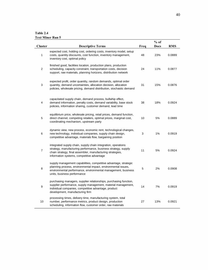
40

Text Miner Run 5

Cluster Descriptive Terms Freq % of Docs RMS

1expected cost, holding cost, ordering costs, inventory model, setup costs, quantity discounts, cost function, inventory management, inventory cost, optimal policy

48 23% 0.0889

2finished good, facilities location, production plans, production scheduling, capacity constraint, transportation costs, decision support, raw materials, planning horizons, distribution network

24 11% 0.0877

3expected profit, order quantity, random demands, optimal order quantity, demand uncertainties, allocation decision, allocation policies, wholesale pricing, demand distribution, stochastic demand

31 15% 0.0876

4capacitated supply chain, demand process, bullwhip effect, demand information, penalty costs, demand variability, base stock policies, information sharing, customer demand, lead time

38 18% 0.0924

5equilibrium price, wholesale pricing, retail prices, demand function, direct channel, competing retailers, optimal prices, marginal cost, coordinating mechanism, upstream party

10 5% 0.0889

6dynamic view, new process, economic rent, technological changes, new technology, individual companies, supply chain design, competitive advantage, materials flow, bargaining position

3 1% 0.0919

7

integrated supply chain, supply chain integration, operations strategy, manufacturing performance, business strategy, supply chain strategy, final assembler, manufacturing strategies, information systems, competitive advantage

11 5% 0.0924

8

supply management capabilities, competitive advantage, strategic planning process, environmental impact, environmental issues, environmental performance, environmental management, business units, business performance

5 2% 0.0908

9

purchasing managers, supplier relationships, purchasing function, supplier performance, supply management, material management, individual companies, competitive advantage, product development, manufacturing firm

14 7% 0.0919

10processing times, delivery time, manufacturing system, total number, performance metrics, product design, production scheduling, information flow, customer order, raw materials

27 13% 0.0921

Table 2.4

41

Run 5 SCM TopicsCluster Topic Area

1 Inventory Management2 Planning and Scheduling3 Demand Management4 Forecasting and Information Sharing5 Contracts and Coordination6 Technology7 Integration8 Business/SC Strategy9 Buyer-Supplier Relationships10 Production-Distribution Systems

Table 2.5

Run 5 SCM Topics – Categorized

Cluster Topic Area5 Contracts and Coordination6 Technology7 Integration8 Business/SC Strategy9 Buyer-Supplier Relationships

Cluster Topic Area1 Inventory Management2 Planning and Scheduling3 Demand Management4 Forecasting and Information Sharing10 Production-Distribution Systems

Table 2.6

Strategic Topics:

Operational Topics:

42

As noted in Table 2.4, the Operational topic clusters contain a greater number of

articles than the Strategic topic clusters. Upon closer inspection of the Operational

topics, it becomes apparent that some of the clusters contain other research areas that

logically fit within these broader topics. For example, both the Planning and Scheduling

topic and the Production-Distribution Systems topic contain articles dealing with

transportation issues, with the majority of the transportation papers falling in the

Production-Distribution category. Additionally, the Inventory Management topic

contains articles that deal with base inventory policies as well as a large number of

articles dealing with inventory modeling and optimization. Both the Operational topic of

Forecasting and Information Sharing, as well as the Strategic topic of Supply Chain

Integration, contain articles dealing with the importance of e-commerce and information

systems. Obviously, these systems are needed to both share information and integrate a

supply chain. The sub-topics that emerge when dissecting the contents of each category

are shown in Table 2.7. These clusters constitute the final results of the Text Miner

analysis of the SCM document corpus. Based on the previous arguments for using these

topics as a proxy for important supply chain design decision areas, we determined that

these clusters and topic area represent the basic general scope of the current literature

and the input into a general supply chain design conceptual model.

43

Modified Run 5 Topic Categorization

Cluster Topic Area5 Contracts and Coordination6 Technology7a Integration Strategy7b e-Commerce Strategy8 Business/SC Strategy9 Buyer-Supplier Relationships

Cluster Topic Area1a Inventory Management Policies1b Inventory Modeling and Optimization2 Planning and Scheduling3 Demand Management4 Forecasting and Information Sharing

10a Production-Distribution Systems10b Transportation

Table 2.7

Strategic Topics:

Operational Topics:

2.5 Discussion

2.5.1 The Supply Chain Design Conceptual Model

The results of the first run of the Text Miner provided us with two main

dimensions found in the SCM literature: supply chain strategy and supply chain

operations. Throughout the subsequent clustering runs, some of the articles moved

between the strategy clusters and the operations clusters. This indicated that there are

many research dimensions that bridge the gap between strategy and operations. Table

2.7 provides the final results of the Text Mining analysis. We listed the ten main supply

chain design dimensions and the three sub dimensions that were discovered. While the

classifications of the categories may seem intuitive, it is important to remember that they

44

have been identified using a quantitative approach to surveying a corpus of literature.

These categories reveal what is being studied and researched in the academic community

regarding supply chain management. From this analysis, we see that the proportion of

Operational topics is significantly greater than that of the Strategic topics. The analysis

also reveals what is not currently being researched on a grand scale. For example,

facility layout research did not emerge as a major topic of current SCM research.

Therefore, we researchers assert that these SCM categories are suitable inputs into a

conceptual model of critical supply chain design dimensions.

The identification of these dimensions is the first step in aiding the development

of supply chain design theories. However, the dimensions alone do not constitute a

conceptual model as defined by Meredith (1993). Therefore, one of the contributions of

this research is the proposal of a Supply Chain Design Conceptual Model (SCDCM).

We will now consider the 13 SCM categories as the 13 supply chain design

dimensions along with the explanation of their place among the SCDCM. The graphical

representation of the model can be seen in Figure 1. The two main categories from the

Text Mining analysis serve as initial basis for the conceptual model. Thus, the logical

space for supply chain design can be divided into two sub-spaces: Strategy and

Operations. Figure 1 indicates that although these two sub-spaces are independent of

one another, they are closely held within the supply chain design space.

The arrows between the Strategy and Operations sub-spaces indicate that the two

areas influence each other and very few decisions can be made in one area that don’t

affect the other. Additionally, the dimensions that are specific to a certain sub-space are

45

located to represent how closely related the design dimensions are to the other sub-

space. The relationships are derived from the observations of the different articles that

“moved” between the Strategy and Operations sub-spaces from one Text Mining run to

the next. For example, the articles that were placed in the Business / Supply Chain

Level Strategy dimension in the Strategy sub-space never crossed over into dimensions

located in the operations sub-space. Likewise, Inventory Modeling and Optimization

papers rarely intermingled with the Strategy dimensions.

However, a number of papers moved between the sub-spaces depending on the

number of clusters requested from the Text Miner. As we noted earlier, the e-Commerce

dimension was found within both the Integration dimension of the Strategy sub-space

and the Forecasting and Information Sharing dimension of the Operations sub-space.

This was also true for Technology articles. Consequently, the SCDCM shows the

majority of the e-Commerce and Technology dimensions resting in the Strategy sub-

space while extending into the Operations sub-space to interact with the Forecasting and

Information Sharing dimension.

46

We have shown that the Strategy and Operations sub-spaces of the SCDCM influence

one another directly through a couple of different dimensions. All of these dimensions

influence the design of a supply chain and so affect one another. This conceptual model

provides visualization into the difficult nature of making supply chain design decisions.

Very few of these decisions can be made in isolation without impacting the supply chain

as a whole, and thereby impact supply chain performance.

The SCDCM provides a starting point for both supply chain design theory

development and applied supply chain design for new products and ventures in the

business world. At this point, our model does not possess explanatory power. It

describes the theoretical view of supply chain management and uses this view as input

data for defining the decision areas deserving of consideration when trying to design a

supply chain that will allow a set of organizations to profitably provide a product or

service.

In the next section of this paper we compare the model that has been uncovered

through the use of text mining on the SCM body of literature with some of the current

models of supply chain management found in academic learning institutions.

47

Supply Chain Design

Strategy Operations

Contracts /Coordination

Business / SCLevel Strategy

IntegrationStrategy

e-Commerce

Technology

Buyer-SupplierRelationships

Inventory MgmtPolicies

Inventory ModelingAnd Optimization

Planning andScheduling

DemandManagement

Forecasting /Information Sharing

Production –Distribution

Transportation

Fig 2.1. Supply Chain Design Conceptual Model

Supply Chain Design

Strategy Operations

Contracts /Coordination

Business / SCLevel Strategy

IntegrationStrategy

e-Commerce

Technology

Buyer-SupplierRelationships

Inventory MgmtPolicies

Inventory ModelingAnd Optimization

Inventory MgmtPolicies

Inventory ModelingAnd Optimization

Planning andScheduling

DemandManagement

Forecasting /Information Sharing

Production –Distribution

Transportation

Production –Distribution

Transportation

Fig 2.1. Supply Chain Design Conceptual Model

48

2.5.2 Current Framework Comparisons

Within business schools across the United States, the concept of supply chains

and supply chain management is presented in a variety of ways. Traditional Operations

Management classes are introducing the notion of Supply Chain Management as a

fundamental topic for graduates to understand. Terms like “Supply Chain

Management,” “Supply Chain Design,” and “Supply Chain Strategy” are being used

interchangeably with the concept of Operations Management. However, the list of SCM

topics derived in this paper for inclusion in the Supply Chain Design Conceptual Model

(SCDCM) represent the concepts and topics that academics are researching under the

SCM umbrella. We contend that if the list of discovered design dimensions is important

in an academic research setting, then those discoveries should also be important in an

academic learning environment.

We will now look at three contemporary supply chain frameworks for

comparison against the thirteen dimensions discussed in the previous section. By

mapping these research findings to frameworks used in general SCM courses, we can

hopefully explore and reconcile gaps between the conceptual design dimensions and

these frameworks. The three frameworks come from common textbooks used in

business schools. While the number of OM/SCM books is quite large, we limited our

comparison to texts using the term “Supply Chain” in the title. OM books will not be

compared in this study.

The three supply chain text books utilized for this comparison of frameworks are:

first, Simchi-Levi, Kaminsky and Simchi-Levi’s book Designing and Managing the

49

Supply Chain; second, Chopra and Meindl’s text Supply Chain Management, Strategy,

Planning and Operations, second edition; and third, Supply Chain Strategy by Frazelle.

Table 2.8 details the key concepts in each of these frameworks as derived by the table of

contents and chapter content of each book.

Current Supply Chain Management FrameworksSimchi-Levi, Kaminsky, and Simchi-Levi Chopra and Meindl Frazelle

Logistics Network Configuration SC Strategy Logistics Performance MeasuresInventory Management Designing the SC Network Customer Relationship ManagementValue of Information Forecasting Inventory ManagementDistribution Strategies Planning Supply ManagementStrategic Alliances Inventory Management TransportationInternational Issues Sourcing Warehouse OperationsCoordinated Product and SC Design Transportation Information SystemsCustomer Value and SCM ContractsInformation Technology for SCM Technology and the SCDSS for SCM E-business

Table 2.8

The Simchi-Levi, Kaminsky and Simchi-Levi (S-K-S) framework is fairly

comprehensive. The Logistics Network Configuration is an attempt to put physical

boundaries on the supply chain by looking at transportation issues, warehouse costs and

capacities and service level demands. This is a one-dimensional approach to supply

chain design. The S-K-S concept of Inventory Management is straightforward, as are

the Distribution Strategies and Information Technology concepts. The Value of

Information refers to Information Sharing and its impact on the Bullwhip Effect.

Strategic Alliances touches on supplier integration. International Issues raises one set of

business strategy concerns in the supply chain. Coordinated Product and SC Design also

touches on supplier integration as well as production strategies. Decision Support

Systems in SCM is an attempt to discuss the impact of one technology on the supply

50

chain. The Customer Value and SCM concept is an indirect attempt to discuss business

level strategy and supply chain strategy. However, the attempt is not in the same vein as

the strategy papers found in the strategy clusters.

The Chopra and Meindl (C&M) framework is the most complete of the three

frameworks, touching on 12 of the 13 supply chain design dimensions we uncovered

during this study. This framework does not delve as deeply into the supply chain

optimization and process modeling component as the current SCM literature so heavily

emphasizes. Otherwise, the Supply Chain Management principles and concepts in the

C&M framework touches on the majority of the design dimensions previously discussed.

The key difference between the ideas presented in the C&M framework and the design

dimensions we focus on in this paper is an on-going concern. The C&M framework

looks at the decisions as modifications to existing problems whereas the SCDCM must

look at these decision areas as inputs into a new supply chain design.

The Frazelle framework is the least complete of the three when compared to the

dimensions of the SCDCM. Although the book is titled Supply Chain Strategy, we find

the framework to have a heavy logistics focus. The framework is centered on production

and distribution strategies and systems, inventory management, information systems in

logistics, and a look at buyer-supplier dynamics. We propose that this framework

provides a good example of an overuse of the term “supply chain” when referring to a

single component of the supply chain.

None of the frameworks explored here presented concepts, ideas or principles

that are not covered by the supply chain design dimensions uncovered in the previous

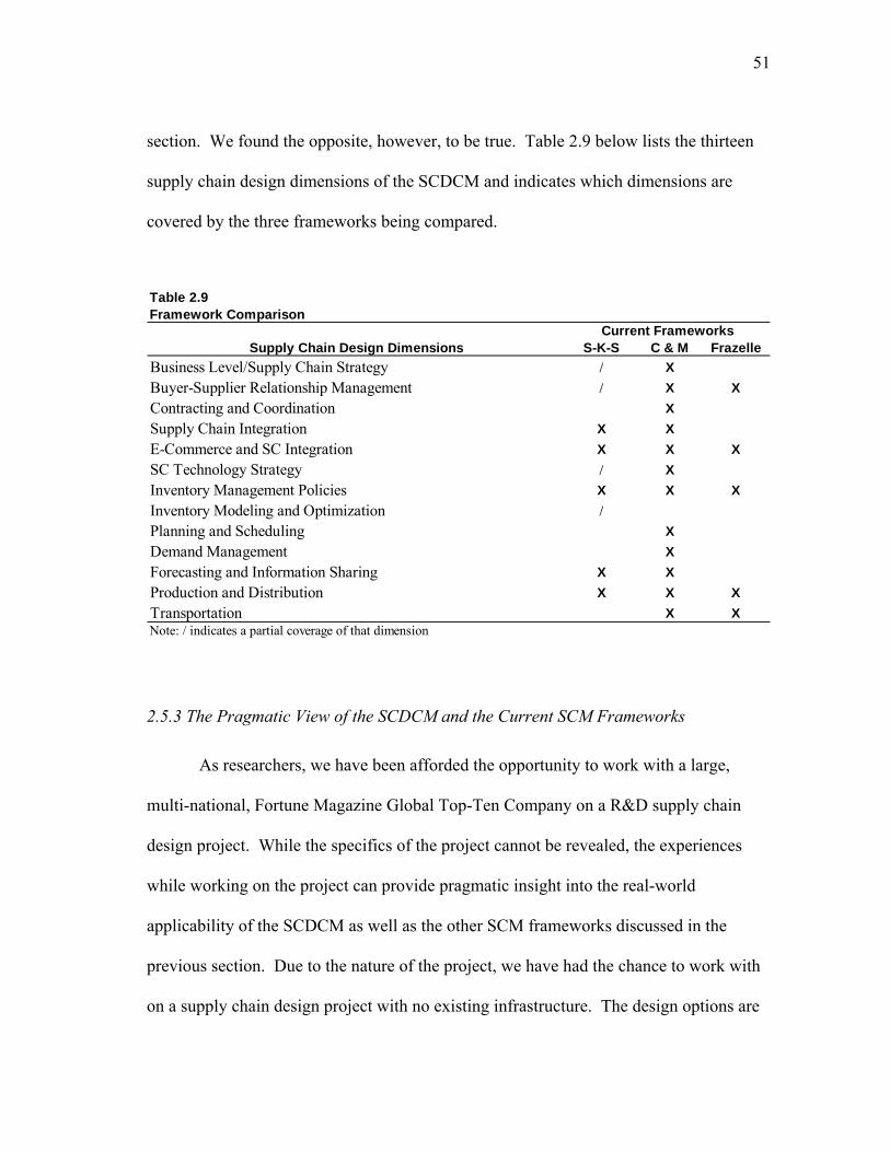
51

section. We found the opposite, however, to be true. Table 2.9 below lists the thirteen

supply chain design dimensions of the SCDCM and indicates which dimensions are

covered by the three frameworks being compared.

Framework Comparison

Supply Chain Design Dimensions S-K-S C & M FrazelleBusiness Level/Supply Chain Strategy / XBuyer-Supplier Relationship Management / X XContracting and Coordination XSupply Chain Integration X XE-Commerce and SC Integration X X XSC Technology Strategy / XInventory Management Policies X X XInventory Modeling and Optimization /

Planning and Scheduling XDemand Management XForecasting and Information Sharing X XProduction and Distribution X X XTransportation X XNote: / indicates a partial coverage of that dimension

Current Frameworks

Table 2.9

2.5.3 The Pragmatic View of the SCDCM and the Current SCM Frameworks

As researchers, we have been afforded the opportunity to work with a large,

multi-national, Fortune Magazine Global Top-Ten Company on a R&D supply chain

design project. While the specifics of the project cannot be revealed, the experiences

while working on the project can provide pragmatic insight into the real-world

applicability of the SCDCM as well as the other SCM frameworks discussed in the

previous section. Due to the nature of the project, we have had the chance to work with

on a supply chain design project with no existing infrastructure. The design options are

52

limited only by product characteristics and imagination. From this project, a number of

applied supply chain design questions have been raised. We have determined that the

answers for many of these questions are not readily available. In this section, some of

these questions are generically discussed and shortfalls between the desired answers and

the SCDCM, the S-K-S, C&M, and Frazelle frameworks are identified.

Although these questions stem from a pure supply chain design project, i.e. a

supply chain that does not currently exist, these questions can be applied to an existing

supply chain in a redesign setting. While a project of this magnitude assuredly generates

hundreds, if not thousands, of unique supply chain design questions, through this

research we present five main questions that have proven to be quite difficult to answer.

Below, we address each question individually, detailing any sub-questions that arise.

These questions are:

1. When designing a supply chain, how many stages should be included in the

design?

2. How many suppliers per raw material/subassembly should each stage have?

3. Who should own/control each stage in the supply chain?

4. What is the appropriate interplay between Intellectual Property Rights and

Outsourcing?

5. When insufficient capacity exists at any stage in the supply chain, should

investments be made in existing suppliers or should the chain consider greenfield

construction?

53

The first question is an issue of supply chain length and complexity. When

designing a supply chain, one must understand the complexity of the task at hand.

Theoretically, supply chains could begin with the extraction of natural resources and end

with delivering a product to the final consumer. In some cases, a supply chain could

begin with the companies that build the equipment to extract the natural resource. Tied

to this question is the perspective one should take when designing the supply chain,

meaning, “Whose supply chain is it?” Wal-mart’s supply chain would most likely look

very different if Procter and Gamble would have been in charge of designing their

supply chain.

The answer to this question is not a simple one, nor is it known. So many factors

are involved in determining the number of stages to consider, such as buyer-supplier

power and global market share, to name a few, that the answer will differ for each

supply chain design project. The answer to this question is mostly the development of a

process which provides a set of key constraints for a company to consider before making

this decision. We recognize through this study that the SCDCM does not have adequate

explanatory power to answer this question. None of the other frameworks discussed in

the previous section deal with this issue either. This topic is ripe for further academic

research.

The second question regarding how many suppliers to have per product per stage

can be looked at from a “portfolio diversification” standpoint. We acknowledge that

having a single supplier ties the hands of the buyer. Given that the number of suppliers

should be greater than one, the question of how many suppliers should each stage have is

54

still unknown. Once again, this is a very complex question with potentially many

complex answers. To the best of our knowledge, there is no magic formula to calculate

the answer to this problem. Generically speaking, this is a Business/Supply Chain Level

Strategy question. However, none of the frameworks, or the SCDCM, can currently

tackle this problem.

The third question deals with stage ownership and control questions. In most

instances, it is not feasible for a single entity to own the entire supply chain. However,

in some cases it may be more feasible for a company to own more than one stage of the

supply chain. Accompanying this question is the notion of stage control. For example,

it may be feasible for a company to own a particular stage in the supply chain while

subcontracting out the control and operation of that particular stage. In other cases, a

third party may own a certain stage of the supply chain, but the company designing the

chain may want to put certain people and processes in place to effectively control that

stage of the chain. What is the interplay between stage ownership and stage control?

We determined that the academic community currently has little to offer on the matter.

While these issues are likely to come up in the dimension of Contracts and Coordination

found in both the SCDCM and the C&M framework, neither of these models provide

answers to this question.

The fourth question centers around the trade-offs between protecting intellectual

property rights and the value of outsourcing. The idea of IP protection vs. outsourcing

falls into the dimensions of Buyer-Supplier Relationships and Contracting and

Coordination. All of the models/frameworks present some type of Buyer-Supplier

55

Relationship dimension with the SCDCM and C&M framework also presenting a

Contracts and Coordination dimension. Our investigation into these models and

frameworks reveals no answers regarding IP and outsourcing. It is possible that these

issues have been left to the jurisprudence literature to handle; however, we concur that

these are very important issues that directly affect the design of a supply chain.

The last question deals with supply chain stage capacity. If a certain stage in the

supply chain is found to lack sufficient capacity to meet the needs of the supply chain, a

couple of different alternatives exist. First of all, additional suppliers could be sought

for the material/subassembly in question. However, this is not always possible. When

no other suppliers exist, the supply chain designers must decide whether or not the

existing supplier’s capacity should be expanded or whether or not to expand capacity

through greenfield expansion. Additionally, how does the chain decide who should pay

for the expansion and who should control the expansion? Under what circumstances is it

beneficial for the supplier to foot the bill for the capacity expansion and when should the

designer pay for it? If the supplier pays for the expansion, how should the contracts be

set up in order to reap the rewards for making the investment? If the designer pays for

the expansion, how does he guarantee that the additional capacity will benefit his firm?

Of all of the questions presented, we find some answers to the fifth question in

the SCDCM. Within the Contracts and Coordination dimension, we found articles that

begin to tackle some of these questions. For instance, Gan, Sethi, and Yan (2004) look

at issues of supply chain coordination with risk-adverse agents. While their paper does

56

not directly answer these questions, we can gain insights from such articles to begin to

formulate an appropriate response.

From the pragmatic questions presented in this section, the reader can begin to

understand the types of real-world problems that supply chain designers must face. The

lack of supporting answers in the SCDCM and the other current SCM frameworks

indicates the need for the academic community to look to the business world for new

research domains that will help provide much needed answers to the real world supply

chain design problems. Nevertheless, the SCDCM provides a broad spectrum of design

elements that must be also be addressed when building or redesigning a supply chain.

As such, we believe it is a good starting point for the creation of an explanatory supply

chain design framework.

2.5.4 Contributions

Through this research, we provide four main contributions to the current body of

SCM literature. First of all, this project demonstrates the usefulness of a quantitative

algorithm in dealing with qualitative, unstructured data. Text mining allows the

researcher to efficiently analyze greater amounts of data than traditional literature

reviews. Text mining provides a way to extract themes and ideas from large bodies of

literature while minimizing the subjective input of the researcher. To our knowledge,

this has not been done before in the field of SCM. Additionally, the start list created

from the current SCM document corpus can be used in the future to analyze a larger

number of SCM documents, should the opportunity arise.

57

Secondly, we have provided a comparison of the text mining results with

currently accepted frameworks used to teach supply chain management to business

students. We acknowledge that not every academic has the same interpretation of the

term “supply chain” and that the term has been loosely applied in some instances. Our

results show that the current body of academic literature is researching and reporting on

supply chain concepts that should be considered when designing a supply chain. Next,

we have also provided a conceptual model for the supply chain design elements. This

conceptual model is the first step pushing the development of a supply chain design

framework and theory. Businesses engage in new endeavors that require a new supply

chain design. This conceptual model takes a step in the direction of helping practitioners

understand the important concepts to consider when designing those new supply chains.

Lastly, we looked at the pragmatic approach of supply chain design and

demonstrated the inadequacies of the current SCM models, including the SCDCM that

was derived from current academic research. This comparison indicates the need to look

at practical applications of the knowledge being created in the academic field and the

necessity for finding new academic research streams by examining real world issues.

The conceptual model requires further extensions in order to take the next step in

building a conceptual framework (Meredith, 1993). Right now, the conceptual model

lacks explanatory power. Future research could develop the constructs necessary to

provide the explanatory power for describing the supply chain design process. In the

realm of text mining, we located several opportunities in the SCM literature. Further

research would be capable of determining whether or not the text mining results would

58

differ if only the article abstracts were used in the research rather than the entire

document. As newer text mining tools emerge with greater explanatory power, future

researchers could re-analyze this study to confirm the findings or to find new linkages

between the natures of the clusters.

59

CHAPTER III

ARB: A TOOL FOR COMPARING SUPPLY CHAIN DESIGNS

3.1 Current Issues

In the previous chapter, we developed a framework for looking at the important

dimensions to consider when designing a new supply chain. With all of the complexity

that exists in global supply chains, we have found that numerous designs could be

feasible for a given set of parameters and assumptions. Therefore, it is important to have

tools for comparing alternate supply chain designs.

Much like our investigation into the existence of supply chain design literature,

we are unable to find academic research or industry accepted quantitative methods or

tools for comparing supply chain designs. Lee (2002) describes how a supply chain

must be agile, adaptable and aligned and Fisher (1997) provides a framework illustrating

how to determine whether a business should use an efficient or a responsive supply

chain. While both articles provide insight into how a supply chain should be

competitively positioned, neither article advises how to evaluate the alternatives that

would fit the needs of a supply chain that could be designed using the authors’ insights.

This illustrates the ongoing need for new tools to evaluate supply chain design options.

In looking for tools by which we can compare different supply chain designs, we

recognize the enormity of the task at hand. Supply chains are complex and intricate in

nature with many different sides. For example, supply chains can be analyzed from

various points of view, including financial analysis, operations management, inventory

management, information sharing, and transportation and logistics.

60

The alluded complexities and intricacies of supply chains naturally lead to

analytical models that are mathematically intractable (Arreola-Risa, 1996 Zipkin 2000).

Consequently, researchers have resorted to heuristics and simulation as alternative tools

for the optimization of supply chain designs (Arreola-Risa, 1998; Zipkin, 2000).

Heuristics have been successful for very limited supply chain configurations (one

product or one stage), but are more difficult to develop for multi-stage and multi-product

supply chain designs. We aim to look at slightly more complex supply chains, and

therefore, we opted for using simulation as the tool for comparing supply chain designs.

Simulation models, after all, are only constrained by the ability of the modeler and the

problem being modeled.

3.2 Rationale for Building the ARB Simulator

We considered two options for building and running a simulation model. The

first option was to buy commercially available simulation software (such as ARENA or

Extend) and the second was to build a piece of software from the ground up. We have

chosen the second option. The reasoning follows.

Commercially available simulators offer a great deal of flexibility in terms of

modeling and data collection. Most packages utilize a graphical user interface that

allows the user the ability to select model inputs and outputs without having to

understand a great deal about how the simulator works behind the scenes. Our

investigation into commercially available software discovered that most software

packages provide the user with standard output variables such as mean, standard

deviation, utilization levels and a variety of general outputs. We were unable to find a

61

software package that provided the actual distributions of output variables as well as

other statistics of interest such as the lead-time demand for orders in the system (the

number of demand arrivals after an order is placed and before the order is received at the

distribution center) and the system inventory level distribution (the distribution of the

actual inventory values throughout the simulation). As demonstrated by Arreola-Risa

(1998) and Zipkin (2000), the random variable lead-time demand is the key for

determining optimal base-stock levels and reorder points. Consequently we built a

simulator that could collect the standard output variables as well as other variables of

interest such as lead-time demand. It should be noted that finding the distribution of

lead-time demand requires programming ingenuity. In our case, we creatively used

object-oriented programming to accomplish the task. The simulator is called the ARB

(Arreola-Risa Brann) Simulator and will be referred to from here on as ARB.

The creation of ARB not only serves as a tool to compare supply chain designs in

this research stream, but is also an academic contribution by itself. ARB can be used for

a variety of different design comparisons and to test an array of hypotheses related to

multi-stage production-inventory supply chain designs. The main simulation processing

code for ARB is provided in Appendix B with the remaining code available from the

author upon request.

3.3 The ARB Model

ARB was designed to be a three-stage supply chain that allows for multiple

customers demanding multiple products from multiple distribution centers. The

distribution centers place orders to a single production facility; in addition, the

62

production facility can have multiple parallel machines to accommodate the orders.

Figure 3.1 provides a graphical depiction of the supply chain design model used by

ARB.

Production Stage

Customer

X0X000XOrder Queue

p1

p2

pn

DC 1

p1

p2

pn

DC n

Customer

Fig. 3.1. ARB Three-Stage Supply Chain Model

Production Stage

Customer

X0X000XOrder Queue

p1

p2

pn

DC 1

p1

p2

pn

p1

p2

pn

DC 1

p1

p2

pn

DC n

p1

p2

pn

p1

p2

pn

DC n

Customer

Fig. 3.1. ARB Three-Stage Supply Chain Model

There is no time delay between when a distribution center places an order and

when the order is received and put into the production queue. There is a setup time (τ)

for each order as well as a production time (α) and a transportation time (t) for the order

to reach the distribution center. The manufacturing time (M) for a given order is found

in Equation 3.1. The manufacturing time does not include the transportation time.

),()( M jijjki,j,k Qατω ++= (3.1)

63

In Equation 3.1, i is the distribution center, j is the product, k is the order number,

ω is the waiting time (the time each order spends in the production queue before it

actually gets produced), and Q(i, j) is the order quantity associated with distribution center

i for product j. For simplification purposes, the distribution center-product combinations

will be referred to as items and will be given then notation of Ii,j. It should be noted that

even if the setup and production times are deterministic, the waiting time will still be a

random variable dependent on system congestion when the order arrives and

consequently the manufacturing time will be a random variable with an associated

distribution (Arreola-Risa, 1998). The lead time (LT) for each order is found in equation

3.2.

ii,j,kkji t+= )(),,( MLT (3.2)

In equation 3.2, ti is the transportation time (mentioned above) from the

production facility to distribution center i. Again, even if the transportation time is

deterministic, the manufacturing time is a random variable and therefore so is the lead

time.

For each of the parameters and variables in the manufacturing time and lead time

equations, ARB has multiple settings and distributions to choose from. The choices for

these variables and other settings for the supply chain design are described in the next

section.

3.4 ARB Simulator Capabilities

ARB has three categories of capabilities as well as a number of reporting options.

The first category deals with runtime parameters, the second category deals with supply

64

chain design, or model, parameters and the third category is the economic parameters.

Runtime parameters handle the actual running of the simulator while model parameters

dictate the supply chain design that ARB is simulating. The user is first prompted for

the runtime parameters followed by the model and economic parameters. Table 3.1

contains a list of the runtime, model, and economic parameters.

3.4.1 Runtime Parameters

The runtime parameters include the number of sampling intervals, the interval

length and the warm-up period. ARB is capable of running the same model several

consecutive times and providing the output for each run individually and for the

aggregate run as well. Therefore, the user needs to specify the number of sampling

intervals to run, ranging from one to twenty. The length of each run is entered directly

into the system. The length of each run is restricted between 10 and 10,000,000 time

periods. So for example, for one model the user may simulate three replications (or

sampling intervals) each with one interval length of 1,000,000 periods.

The warm-up period is the number of time periods in which the simulation runs

but the data for the output variables and statistics is not collected, thus allowing the

simulation to get into steady state (Law and Kelton, 1999). The warm-up period is

specified as a percentage of the length of each interval. The warm-up period in ARB is

required to be between zero and 50%. For example, the user may run the simulation for

100,000 time periods with a warm-up period of 10%, in which case the simulation runs

for 100,000 time periods but only collects data from period 10,001 to period 100,000.

65

Table 3.1ARB ParametersParameter Options

Runtime Parameters

Number of Sampling Intervals 1 - 20*Interval Length (periods) 10 - 10,000,000*Warm-up Period 0% - 50%

Model ParametersInfrastructure Parameters

Distribution Centers 1 - 20*Products 1 - 20*Machines 1 - 20*Production Lot Processing unit, batch

Process Parameters

Demand Inter-Arrival Time (1/λ) x > 0Demand Order Size x* ≥ 1Production Time (µ) x > 0Setup Time (τ) x ≥ 0Transportation Time (t) x ≥ 0Reorder Point −∞ < x* < ∞Order Quantity x* ≥ 1Quality Yield 0 < x ≤ 1

Item Parameters

Demand Inter-Arrival Time homogeneous, heterogeneousDemand Order Size homogeneous, heterogeneousProduction Time homogeneous, heterogeneousSetup Time homogeneous, heterogeneousTransportation Time homogeneous, heterogeneousReorder Point homogeneous, heterogeneousOrder Quantity homogeneous, heterogeneous

Economic Parameters

Unit Cost x ≥ 0Holding Cost 0 ≤ x ≤ 1Backorder Penalty x ≥ 0

* Integer values

66

3.4.2 Model Parameters

As conveyed earlier, the supply chain being explored is formed through the

parameters that constitute the model capabilities. These parameters were classified into

three different categories: supply chain infrastructure parameters, supply chain process

parameters, and the item parameters. The infrastructure parameters include the number

of distribution centers, the number of products, the number of parallel machines at the

production facility, and the production lot processing capability. The process parameters

consist of the demand inter-arrival time, demand order size, production time, setup time,

transportation time, reorder point, order quantity, and quality yield. The item parameters

determine whether items, Ii,j for all i and j, are homogeneous or heterogeneous across all

of the process parameters except quality yield.

3.4.2.1 Infrastructure Parameters

The infrastructure parameters, the number of distribution centers, the number of

products, and the number of machines, can range from one to twenty. The production

lot processing capability dictates whether items are produced on a per unit basis or on a

batch basis. The per unit basis indicates that each order is produced one unit at a time

while the batch selection will cause the entire order to be produced collectively in a

single batch (such as an oven operation).

3.4.2.2 Process Parameters

The eight process parameters determine how the supply chain reacts to its

customers and orders. The demand inter-arrival time specifies how often customers

arrive at the distribution center demanding a given product. The demand order size

67

indicates how many products the customer demands when arriving at the distribution

center. Setup time, production time and transportation time parameters indicate how

long it takes to setup the production line in order to make the product, the time necessary

to produce the product, and how long it takes to ship the product back to the distribution

center. The reorder point is the specific inventory level that triggers the placement of an

order from the distribution center to the production facility and the order quantity is the

quantity of product ordered each time an order is placed. The quality yield is an input

that indicates the average percentage yield of the process (the percentage of products

produced that pass “quality inspection” and are placed in inventory at the distribution

center).

The demand inter-arrival time, demand order size, setup time, production time

and transportation time require three inputs: distribution, mean and coefficient of

variation (CV). Demand inter-arrival time, setup time, production time and

transportation time can follow either a discrete or continuous distribution. The only

discrete distribution available in ARB for these four parameters is the deterministic

distribution where each of the process times is fixed at a single time value. Otherwise,

these parameters can be continuously distributed according to a gamma, uniform,

triangular, or normal distribution (an exponential distribution is created by setting the

coefficient of variation for the gamma distribution equal to one (Law and Kelton, 1999)).

The demand order size must be a discrete random variable (it is assumed that production

is of discrete units that can not be broken into parts) and can be distributed according to

a deterministic, Poisson, negative binomial, or uniform distribution. The generation of

68

the random variates is implemented using the procedures found in Law and Kelton

(1999).

The remaining process parameters, reorder point, order quantity, and quality

yield, are single value parameters. The reorder point and order quantity are integer

values that respectively represent the inventory level, when reached, at which an order

will be placed to the manufacturing plant and the size of the order that is placed. The

quality yield parameter determines the average yield of the supply chain for each order.

The options for quality yield are (as percentages): 100, 99, 98, 97, 96, 95, 90, 85, 80, 75,

and 50. Quality yield assumes 100% inspection upon arrival at the distribution center, at

which time the quality yield of each order is determined and only the “good” products

are put into inventory; the defected products are discarded. The details of how this is

implemented will be explained in further detail in a subsequent section.

3.4.2.3 Item Parameters

The last model parameters, the item parameters, determine if and how the items

differ. While quality yield has been modeled at the supply chain level, meaning all

items, Ii,j, experience the same yield percentage, the item parameters can be

differentiated according to the distribution center level, the product level, or both. The

demand inter-arrival time (IAT) and the transportation time are distribution-center

dependent and are therefore able to be differentiated at the distribution center level. This

means that while each distribution center has the same random variable distributions for

the IAT and transportation time, the distribution centers can have different mean and

CVs for these parameters.

69

Setup times and production times are product dependent and can be differentiated

at the product level. Like IAT and transportation time, all products will have the same

setup time distribution and production time distribution with potentially different means

and CVs for each parameter. The demand order size, reorder point, and order quantity

applies to each item on both the distribution center and product level. Therefore, these

parameters can have different means and CVs (demand order size) or integer values

(reorder point and quantity) for each distribution center-product combination.

3.4.3 Economic Parameters

One of the automatic outputs of the ARB is to calculate the base-stock level that

will produce the lowest expected total inventory cost based on expected stockouts,

backorders, and on-hand inventory. In order to do this the model must be provided with

a unit cost, holding cost and a backorder cost or penalty. ARB requires that the user

input a unit cost, the holding cost as a percentage of the unit cost, and the backorder

penalty as a ratio of the backorder cost to the holding cost. If the unit cost is $10, the

holding cost percentage is 20% and the backorder penalty ratio is 4, then holding cost is

$2, and the backorder cost is $8.

3.4.4 Reporting Options

Once the runtime and supply chain design (model) parameters have been

selected, the ARB provides a number of reporting options. In the case where more than

one item is being simulated (more than one distribution center-product combination),

ARB provides the option to report the statistics and distributions for only the first item

70

(I1,1) or for all items. Additionally, there are two categories of statistics and distributions

to choose from: system and item statistics and distributions.

System statistics and distributions consist of the order arrival times into the

production system, the system waiting time, and the system production queue length. In

the case where the simulation is only dealing with one item, the system statistics and

distributions will be identical to the item statistics and distributions for these three

variables. The item statistics and distributions include the item level demand inter-

arrival time, order arrival rate, waiting time, manufacturing time, lead time, lead-time

demand, inventory level, inventory on-hand, inventory backorders, maximum

backorders, stock outs, outstanding orders, setup times, production times, transportation

times, and the demand order size. In the report output, the mean and variance is

provided for each of the variables selected as well as the actual distribution of that

variable. The collection and reporting of these distributions as a group is what separates

the ARB simulator from the commercially available simulators.

3.5 Implementation of Capabilities

With the ARB runtime and supply chain design (model) capabilities having been

described in the previous section, we will now describe how these capabilities are input

into ARB. Upon start-up, ARB requires the runtime parameters be selected before

moving on to the model parameters. The number of sampling intervals is selected from

a drop-down menu that allows the user to select up to 20 sampling intervals (or

consecutive runs with the same supply chain design) with the default being one sampling

interval. The user then enters the length of the sampling interval ranging between 10

71

and 10,000,000 time periods and ARB will inform the user to correct any intervals that

do not lie within this range. The user will then enter the warm-up period as a percentage

of the overall sampling interval. Again, this period must be between zero and 50

percent, entered as a decimal.

Once the runtime parameters are entered, ARB requests the supply chain design

level parameters. These parameters will define the structure of the supply chain as well

as overall distribution types for the process parameters and the supply chain’s quality

capabilities. The user selects the number of distribution centers, the number of products

going to each of the distribution centers, and the number of parallel machines in the

production facility from drop-down menus. These variables range from one to 20

available DCs, products or machines, with the default being one. The user then selects

the production lot processing capability, which can either be “one unit at a time” or

“batch processing,” with the default being “one unit at a time.”

Following the production lot processing capability selection, ARB needs the

distribution selections for the demand inter-arrival times, demand order size, production

times, setup times, and transportation times. These supply chain level variables can be

chosen according to the distributions described for each one of them in the previous

section. The default selection for all of these variables is deterministic. The final supply

chain level variable selection is the quality yield of the production system. This is

selected from a drop-down box that is populated with the values provided in the previous

section. The default value is 100% and all items are assumed to have the same average

72

quality yield due to the fact that they all come from the same production process and

facility.

The item parameters are entered next. The available options depend on the

inputs for the number of distribution centers and the number of products. If the there is

only one distribution center and one product, there is only one item. Therefore, if the

simulation consists of a single item, the item parameters are fixed so that the demand

inter-arrival time, demand order quantity, production time, setup time, transportation

time, reorder point, and order quantity are all homogeneous (by definition, they cannot

be otherwise with only one item). If, however, the user selects to have more than one

distribution center, demand inter-arrival times, transportation times, demand order

quantities, reorder points and reorder quantities can now be heterogeneous. If more than

one product is selected, production and setup times along with demand order quantities,

reorder points and reorder quantities can now be heterogeneous.

Once the homogeneity decisions have been made for the item parameters, the

user must enter the means and CVs (if applicable) for all of these parameters. How these

items are input depend on two previous inputs: the supply chain level distributions and

the homogeneity decisions. For any of the item parameters that were chosen to have a

deterministic distribution, only a mean is required to be entered. The mean would then

represent the exact number for that parameter. For any of the continuous or discrete

(non-deterministic) distributions that were chosen, the user must input a mean and a CV

for those parameters. Again, the reorder point and order quantity are integer values

without an underlying distribution.

73

If all items are homogeneous, the user can input the means, CVs, and integer

values at one time. If the items are heterogeneous, the user will be prompted to enter the

information for the demand inter-arrival times first, followed by the demand order

quantities, production times, setup times, transportation times, reorder points and finally

the reorder quantities. Once the pertinent means, CVs, and integer values have been

input, the user must decide on the statistics to be reported. The selection of statistics can

be selected using the corresponding check boxes. Once this has occurred, the user has

completed the runtime and supply chain design (model) selection process. Before the

simulation can be run, the user must also decide upon the order processing policy for the

production facility and the inventory cost policy for the simulation. These topics are

covered in the next two sections.

3.6 ARB Simulator Order Processing Policy Implementation

In the ARB, we implement three order processing policies: First-Come, First

Serve (FCFS), Longest Queue First (LQF), and Fixed Priority (FP). FCFS was chosen

because it is a very common method for processing work requests in the business world.

LQF is implemented because of the claims that this policy produces lower total

inventory costs than FCFS (Zheng and Zipkin, 1990). FP has been implemented to

allow for comparisons when a single, predominant customer is given preferential

treatment over the other customers.

Our inventory system implements the FCFS rule in the simplest possible manner.

Orders are processed in the sequence in which they are received. This requires no

additional steps to determine which order is next in line. No rearranging of the

74

production queue is permitted under FCFS. The LQF order processing rule looks to see

which item has the greatest number of orders outstanding and then rearranges the

production queue to produce that item next. LQF can be implemented in a number of

different ways.

One of the variations available to LQF is the implementation of preemptive

processing. Under preemptive processing, the system calculates the greatest number of

orders outstanding immediately upon receiving the next order. If the order that was just

received gives item A more outstanding orders than item B, the system will immediately

stop producing item B, if it is being produced, and begin producing item A (Zheng and

Zipkin, 1990). ARB does not implement preemptive processing. Orders currently in

production are allowed to finish once started, even though the state of the system may

have changed. Additionally, production priorities are checked when the manufacturing

machine becomes available and not when an order is placed, thereby coinciding with a

non-preemptive manufacturing policy.

The greatest number of outstanding orders can also be implemented in different

ways. To make this determination, the simulator can look at the actual production queue

or it can look at the inventory level of the distribution center. By looking at the

inventory level at the distribution center, the system can determine the greatest need

based on relative inventory levels.

ARB implements this policy by looking at the inventory level of the distribution

center and not the production queue length. ARB calculates the ratio of inventory level

to the base-stock level and gives priority to the item with the lowest ratio. For

75

homogeneous items, this procedure will produce the exact same result as looking at the

production queue length while providing ARB the opportunity to use a more realistic

measure of inventory “need” in the heterogeneous item case.

ARB implements a third processing rule that we call Fixed Priority (FP). FP

rearranges the production queue based on a predetermined item priority. If item 1 is

given the priority the production system will always give the available machine to item 1

if an order for item 1 exists. Otherwise it will process the remaining items on a FCFS

basis. This order processing rule is equivalent to giving item 1 access to a much faster

production rate than it would have under the other two ordering policies. The main

benefit of this rule is to allow the user to see the impact of giving priority to one main

customer on the manufacturing time and lead time for the other customers.

With any production-inventory system, customers who “show up” and demand a

product only to find out that temporarily there is no product in stock have two options:

wait for the product (create a backorder) or leave and buy the product elsewhere (lost

sales). ARB does not allow any lost sales. Therefore, any unfulfilled orders at the time

of demand become backorders in the system.

As mentioned in the previous section, the order processing policy for a given

simulation run is selected after the runtime and model parameters have been input. The

order processing policy options are also controlled by the number of items in the system.

If only one item is specified (one distribution center-product combination), then FCFS is

the only option. If more than one item is specified, the user can then choose between

FCFS, LQF, and FP. If FP is selected, the user must then determine which of the items

76

receives priority. Once the order processing rule has been chosen, the user must

determine the inventory cost policy. This policy is covered in the next section.

3.7 ARB Simulator Inventory Cost Policy Implementation

Hadley and Whitin (1963) present two different methods by which to charge for

backorders: per unit backordered and per unit per unit time backordered. In ARB, the

per unit backorder cost is labeled as p and the per unit per unit time is labeled as π. The

expected total inventory cost (E(Kp)) for a base stock policy that penalizes backorders

using p is defined by Equation 3.3, where E(OH) is the expected amount of on-hand

inventory, h is the holding cost percentage, C is the unit cost, P(SO) is the probability of

a stockout, p is the previously defined backorder penalty, T is a time-based factor to

convert from the prevailing time period assumption to a cost-based time basis that is

compatible with the one selected for h (e.g. to convert from a daily basis to an annual

basis), and λ is the demand inter-arrival time.

1 −⋅+⋅= λΤpP(SO)hCE(OH))E(K p (3.3)

Equation 3.3 shows that the total inventory cost associated with a given base

stock policy with a per unit backorder penalty is the combination of the holding cost for

the expected on-hand inventory plus the backorder penalty that results from multiplying

the probability of being out of stock times the demand rate per time period, adjusted if

necessary for obtaining the cost in a different time basis than the simulation assumes,

times the penalty paid for being out of stock. In this case, using p as the backorder

penalty policy, E(Kp) can be interpreted as the expected cost for implementing a certain

base stock policy over an infinite-time horizon.

77

If a policy is chosen that penalizes backorder per unit per unit time, the expected

total inventory cost function changes as does the interpretation of the penalty. This

policy is analogous to working a job that pays an hourly wage. If you work for half the

day (four hours), you are paid for only half the day. Therefore, if a customer arrives at

the distribution center demanding a certain item that is backordered, the customer will

receive compensation for waiting as long as necessary to receive the item. If π is $10 a

day/unit and the customer waits for two days, the customer receives $20 in

compensation. On the other hand, if the customer only waits half a day then he receives

$5 in compensation. Under the p policy, if p is $10 the customer would receive a flat

$10 in compensation regardless of waiting time.

The expected total inventory cost under π, i.e. E(Kπ), is defined in Equation 3.4.

Like Equation 3.3, the holding cost is calculated using the expected on-hand inventory,

the holding cost percentage and the unit cost. The backorder penalty is calculated as the

expected number of backorders (E(BO)) times the penalty cost π. Once the simulation

has reached steady state, the expected number of backorders at a single moment in time

or over any number of time periods is the same. Therefore, the expected penalty paid

per unit per unit time is simply E(BO)⋅π. The units of hC and π must match.

ππ ⋅+⋅= E(BO)hCE(OH))E(K (3.4)

On a related matter, there is no direct way to compare the expected costs of the

two backorder penalty policies. One can be given in terms of the backorder penalty paid

over a specific time period and the other is the average amount paid over any time period

in question. Once the unit cost, holding cost percentage and backorder cost to holding

78

cost ratio is input, ARB will calculate the base-stock level that minimizes the expected

total inventory cost under both p and π for all items in the simulation and will report the

optimal base-stock level and its associated minimum expected cost for both penalty

scenarios. These expected total inventory costs can be used to directly compare supply

chain designs and order processing policies.

3.8 ARB Simulation Process

ARB runs following two distinct processes: the setup process and the simulation

process. Most of the setup process has been described in the previous sections. The

setup process flow can be seen in Figure 3.2. The final setup steps that are not

mentioned above are the simulation initialization steps including initializing the

simulator, initializing the statistical counters and variables, the creation of the initial

demand events for all items and the firing of the main simulation routine.

The simulation process used by ARB follows the general simulation steps

outlined in Law and Kelton (1999). The unique characteristics of the ARB process are

outlined in Figures 3.3 and 3.4. The process begins with grabbing the first event in the

event queue. This event is checked to see if the simulation should be terminated. If the

event is a termination event, the simulation queues are cleared, the statistics are

collected, the output reports are generated, and the simulation is terminated. If the event

is not a cue to stop the simulation, the process checks to see if it is still in the warm-up

period attempting to reach steady state. If the simulation is still running in warm-up

mode, no statistics are collected. If not, the global simulation statistics are collected.

Then the simulator determines what type of event it has removed from the event queue.

79

There are only four production-inventory events: DEMAND, ORDER,

PRODUCTION_DONE, and SHIPMENT. Depending on the event type, the process in

Figure 3.3 continues with the appropriate node on Figure 3.4.

Fig. 3.2. ARB Setup Process Flow

80

Fig. 3.3. ARB Simulation Process Part 1

81Fig. 3.4. ARB Simulation Process Part 2

82

DEMAND events indicate a customer has arrived at the distribution center

demanding an item. The system checks to see if the distribution center has any

inventory. If it does not, ARB records the stockout situation. ARB then determines how

many items the customer is demanding using the distribution that was specified for the

demand order size. For each item demanded, the inventory level is decremented and the

appropriate lead-time demand statistics are collected for the system. ARB also

determines whether or not an order is created for each item demanded. If the demand

causes an order to be generated, the ORDER event is created and place in the event

queue. Next the system creates the next DEMAND event for the current item. If the

system is not in warm-up mode, the appropriate statistics are collected. ARB then

returns control to the main loop which updates the current “clock” and pulls the next

event from the event queue (The return arrows at the end of the DEMAND loop to the

top of Figure 3.4 indicate a return to Figure 3.3).

The ORDER event indicates that an order has been placed to the

production/manufacturing facility. The ORDER event causes an order for the

appropriate item to be created and ARB records the arrival time of the order into the

system. Depending on the order processing rules, the order is assigned a priority within

the production queue. The number of outstanding orders is incremented and ARB

checks to see if there is a free production machine. If there is a free machine, the order is

produced immediately with the appropriate setup and production distributions and times

being generated. The production of the order creates the PRODUCTION_DONE and

SHIPMENT events and places those events in the event queue. If a machine is

83

unavailable, the order is placed in the production queue to wait its turn. The ORDER

event returns control to the main loop. The main loop then updates the current “clock”

and pulls the next event from the event queue.

The PRODUCTION_DONE event causes the order associated with this event to

be deleted from the production queue and checks the system to see if there are any

orders waiting to be produced. Depending on the order processing policy selected, the

orders are prioritized and the order with the highest priority is selected for production.

The production routine is called and the PRODUCTION_DONE and SHIPMENT events

are created for the next order. Control is then returned to the main loop.

The SHIPMENT event indicates that an order has reached the distribution center.

If the system is not in the warm-up period, all of the statistics for the order and shipment

are collected and the items undergo 100% inspection. The outcome of this inspection is

determined using the quality yield input. For a given order, each item in the order is

tested for quality using Law and Kelton’s (1999) procedure for generating random

Bernoulli variates. A uniform random number is generated. If that number is less than

or equal to the quality yield percentage, the item passes inspection. If it is larger than the

quality yield percentage that item fails inspection. The inventory level for the items

received is then incremented by the number of “good” items. The number of

outstanding orders is decremented and the order is removed from the system. Control is

then returned to the main loop.

This process continues until the simulation interval length has been reached.

Once the simulation stop time is reached the termination routine is executed. The output

84

files are written and the simulation stops. At this point, the output is ready for analysis.

The size of the ARB code precludes it from all being placed in the appendix of this

document. However, we reiterate that the main code for ARB is included in Appendix B

and the remaining code can be obtained by contacting the author.

3.9 Testing the ARB Model

We first verified that the random number generators included in the ARB Model

were working properly, by performing a battery of simulations. The results of these

simulations are available from the author upon request. However, given the importance

of the exponential random variable in our work, we decided to include the test for this

distribution in Table 3.2. The simulator was run using exponentially distributed demand

inter-arrival times (0.5 periods between arrivals, or equivalently 2 arrivals per time

period). The distribution for these inter-arrival times was captured from the output and

compared to the analytical results for an exponential distribution. As can be observed in

that table, the analytical and simulated results match.

We next proceeded to test the model logic. To do so, we decided to replicate in our

model a system with well-known analytical results, the steady-state M/M/1 queuing

system, by using the following settings:

1) Number of distribution centers: 1.

2) Number of products: 2.

3) Number of parallel machines: 1.

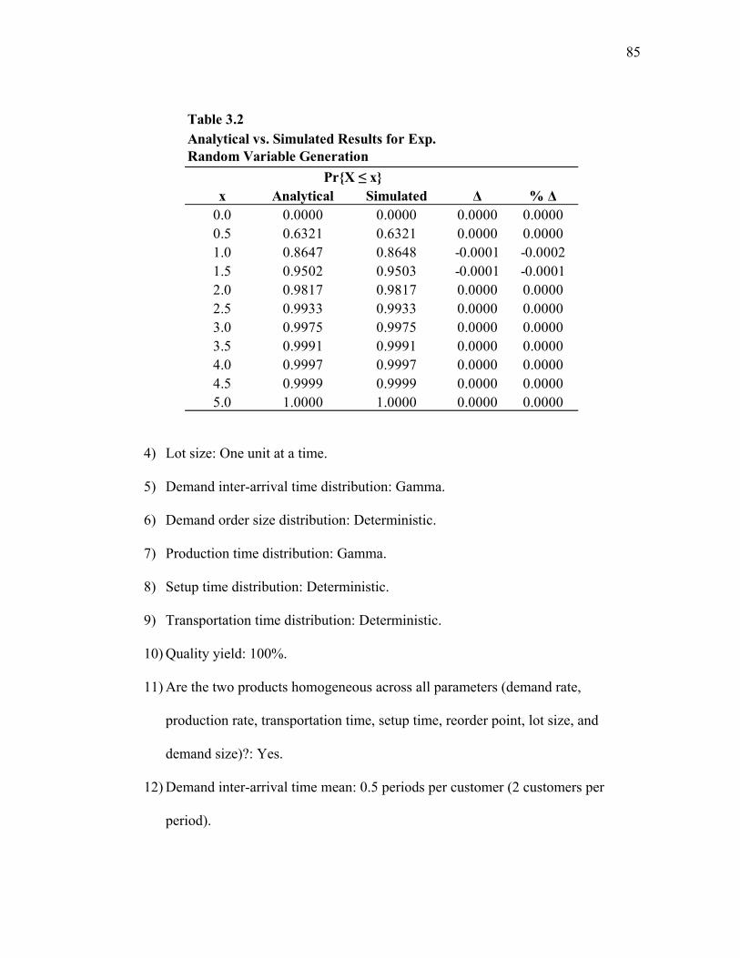
85

Table 3.2

x Analytical Simulated ∆ % ∆0.0 0.0000 0.0000 0.0000 0.00000.5 0.6321 0.6321 0.0000 0.00001.0 0.8647 0.8648 -0.0001 -0.00021.5 0.9502 0.9503 -0.0001 -0.00012.0 0.9817 0.9817 0.0000 0.00002.5 0.9933 0.9933 0.0000 0.00003.0 0.9975 0.9975 0.0000 0.00003.5 0.9991 0.9991 0.0000 0.00004.0 0.9997 0.9997 0.0000 0.00004.5 0.9999 0.9999 0.0000 0.00005.0 1.0000 1.0000 0.0000 0.0000

Pr{X ≤ x}

Analytical vs. Simulated Results for Exp. Random Variable Generation

4) Lot size: One unit at a time.

5) Demand inter-arrival time distribution: Gamma.

6) Demand order size distribution: Deterministic.

7) Production time distribution: Gamma.

8) Setup time distribution: Deterministic.

9) Transportation time distribution: Deterministic.

10) Quality yield: 100%.

11) Are the two products homogeneous across all parameters (demand rate,

production rate, transportation time, setup time, reorder point, lot size, and

demand size)?: Yes.

12) Demand inter-arrival time mean: 0.5 periods per customer (2 customers per

period).

86

13) Demand inter-arrival time coefficient of variation (CV): 1.

14) Demand order size: 1.

15) Unit production time: 0.225 periods (4.44 units per period).

16) Coefficient of variation (CV) of demand inter-arrival time: 1.

17) Setup time: 0.

18) Transportation time: 0.

19) Distribution center Order lot size: 1.

20) Distribution center reorder point: 0.

21) Order processing rule: FCFS.

To determine the number of demand arrivals needed to reach steady-state is a

well-known problem in simulation. An excellent treatment of this problem can be found

in Whitt (1989). In his seminal paper, Whitt suggests that for M/G/1 queueing systems,

to achieve a given relative standard error (defined as the ratio of standard deviation to

mean) and confidence level in the steady-state simulation results, the number of demand

arrivals should be n, where

222

22/

2

)1()1(8

ερρβ

−

+=

zcn s (3.5)

and 2sc is the squared coefficient of variation of service times, 1 – β is the confidence

level, zβ/2 is the z value providing and area β/2 in the upper tail of the standard normal

probability distribution, ρ is the capacity utilization level, and ε is the relative standard

error.

87

Hence for the M/M/1 queuing system under consideration, for a relative standard

error of 0.05 and a 95% confidence level, the minimum required number of arrivals

should be 3,160,494. Consequently, and because the demand arrival rate per period was

set at 2 per period for each product, we decided to simulate the system for one million

periods, yielding a total of 4 million arrivals, which exceeds the minimum number

suggested by Whitt.

The steady-state cumulative distribution function (CDF) of waiting time in queue

(Wq) for an M/M/1 queuing system is given by (see, for example, Gross and Harris

(1985))

µρ / 1)Pr( xq exW −−=≤ (3.6)

where 1/µ is the unit production time. The exact and simulated cumulative distribution

functions (CDFs) for the system being replicated are provided in Table 3.3.

We next tested the following null hypothesis: The exact and simulated CDFs are

equal, against the alternative hypothesis: The exact and simulated CDFs are not equal.

Such a test was conducted using the Kolmogorov-Smirnoff methodology (Johnson and

Wichern, 2007). Of the 4 million demand arrivals, we selected the last 100,000 and

measured their waiting time in queue. We then tested for correlation among the observed

waiting times. Given that the Kolmogorov- Smirnoff test assumes independent

observations, we determined, using brute force and Excel, that to obtain independent

waiting times in queue we had to select waiting times in queue that were 500

observations apart. This left a total of 2,000 observations for the Kolmogorov-Smirnoff

test. The calculated p value of the test was 0.75 which clearly cannot be used to reject

88

the null hypothesis. The two most important conclusions from this test are the

following:

1) There is no reason to suspect the model logic is incorrect.

2) Based on Whitt’s (1989) results, Equation 3.5, and our test results, at least 4

million demand arrivals are needed to achieve steady-state results when

production times are exponentially distributed. This conclusion will be used later

in the dissertation.

Table 3.3Comparison of M/M/1 Results

x Analytical Simulated ∆ % ∆

0.0000 0.1000 0.1006 -0.0006 -0.00600.4500 0.2630 0.2646 -0.0016 -0.00610.9000 0.3965 0.3990 -0.0025 -0.00631.3500 0.5058 0.5084 -0.0026 -0.00521.8000 0.5953 0.5976 -0.0023 -0.00392.2500 0.6686 0.6703 -0.0017 -0.00262.7000 0.7286 0.7298 -0.0012 -0.00163.1500 0.7778 0.7783 -0.0005 -0.00073.6000 0.8180 0.8185 -0.0005 -0.00064.0500 0.8510 0.8517 -0.0007 -0.00094.5000 0.8780 0.8787 -0.0007 -0.00084.9500 0.9001 0.9008 -0.0007 -0.00085.4000 0.9182 0.9189 -0.0007 -0.00085.8500 0.9330 0.9333 -0.0003 -0.00036.3000 0.9451 0.9452 -0.0001 -0.00016.7500 0.9551 0.9549 0.0002 0.00027.2000 0.9632 0.9628 0.0004 0.00047.6500 0.9699 0.9694 0.0005 0.00058.1000 0.9753 0.9748 0.0005 0.0005

>8.1000 0.0247 0.0252 -0.0005 -0.0206

Total 1.0000 1.0000

Pr(Wq ≤ x)

89

We re-emphasize that ARB not only aids in the supply chain design research

contributions of this dissertation but is also an academic contribution by itself. The

collection and reporting of the non-standard statistical distributions, the built-in order

processing rules, and the associated base stock policy economic analysis make ARB

unique in the realm of off-the-shelf simulators. This simulator represents new

capabilities for comparing production-inventory supply chain designs.

90

CHAPTER IV

COMPARING SUPPLY CHAIN DESIGNS

4.1 Supply Chain Design Complexity

In Chapters II and III, we have established the fact that supply chains are

complex networks of firms (Christopher, 1998; Stadtler, 2005) dealing with the physical,

financial, and information flows (Sahin and Robinson, 2002) between all stages in the

chain in order to increase the overall profitability of the chain (Chopra and Meindl,

2004). The complexity inherent in supply chain management increases when designing

or redesigning a supply chain. Our conceptual model of supply chain design identified a

minimum of thirteen design dimensions that need to be taken into account when creating

a supply chain design. Within these dimensions there are numerous angles to attack the

design possibilities.

Within the Business/Supply Chain Strategy category there are several strategies

to consider. Supply chain designs must match the operating strategy and competitive

priorities (Boyer and Lewis, 2002) with product types (Christopher and Towill, 2002).

Management must also decide on environmental strategies (Angell and Klassen, 1999;

Bowen, et. al., 2001; Zhu and Sarkis, 2004), purchasing strategies (Chen, Paulraj, and

Lado, 2004), and information strategies (Techmistocleous, Irani, and Love, 2004) to

name a few.

In the Buyer-Supplier Relationship category, we learn of the importance of

designing the correct power relationships (Benton and Maloni, 2005), the effect of

service quality along the supply chain (Stanley and Wisner, 2001), and the impact of

91

supplier evaluation strategies on supply chain performance (Prahinski and Benton,

2004). The Planning and Scheduling category includes logistics scheduling problems

(Bertazzi and Speranza, 1999), the impact of advanced planning systems on the supply

chain (Stadtler, 2005) and the need to optimize lot sizing for scheduling purposes

(Kaminsky and Semchi-Levi, 2003) to list a few of the design consideration areas.

Each of the design categories can be broken down into several sub-categories and

topics which demand consideration when building a supply chain. The reality of

building all of these concepts simultaneously and being able to factor in the impact that

one decision has on another would be near impossible. The best we can do is isolate one

or more of these issues at a time and look to see how these issue affect one another and

how to achieve the best supply chain design possible given the constraints of each

unique situation. Along those same lines, it would be very difficult to compare supply

chain designs if several parameters for the designs differed between the chains under

comparison. Given the development of the ARB simulator described in the previous

chapter, our research looks to use ARB as a tool to compare supply chain designs. To do

this effectively we decided to focus this research on the impact of the use of real-time

information on order processing rules in a production-distribution environment.

4.2 The Use of Real-Time Information in a Production-Distribution Environment

Much has been said about information sharing in the operations management and

supply chain management literature (Ketzenberg, et.al., 2007; Ferguson and Ketzenberg,

2006; Ketzenberg, et.al., 2006; Sahin and Robinson, 2002). Accurate, up-to-date

information is needed in the business world to facilitate decision making at all levels of

92

an organization. It has become a given that real-time information, when available, can

prove valuable to a company.

In their 1990 paper, Zheng and Zipkin provide analytical proof that using real-

time information can provide lower total inventory costs when applied to a production

environment. They compare two supply chain designs that differ solely based on the use

of real-time information. The first supply chain design does not use real-time

information to update the sequence of customer orders through the production facility.

The design uses a first-come, first-serve approach (FCFS) to process customer orders.

The authors believed that using real-time information to alter the sequence of the

production of customer orders could improve the expected amount of on-hand inventory

while reducing the number of expected backorders and lower the probability of the

customer experiencing a stockout.

To implement the second supply chain design, Zheng and Zipkin (1990) looked

at a ready source of real-time information: the production queue length for different

customer orders. By determining which customer had the greatest number of orders in

the system, the sequence of order production could be altered to give priority to the

customer with the greatest number of orders. By giving priority to that customer’s order

the lead-time would be shortened, on-hand inventory would rise, backorders would

decrease, and the probability of the next customer experiencing a stockout is lowered.

The authors refer to this real-time information order processing policy as the longest

queue first (LQF) policy.

93

Zheng and Zipkin (1990) assume a very basic supply chain design for their

analysis. The supply chain consists of customers, a single distribution center, and a

single stage production facility with no raw material constraints. They analyze the chain

assuming two (homogeneous) products with identical Poisson demand rates. Both

products utilize the same production facility and the facility can only manufacture one of

the two products at a time. The economic factors between the products are identical and

the production rate for both products is an exponentially distributed random variable

with a mean production rate greater than twice the demand rate. The products do not

have setup times or transportation times. Additionally, the order processing policy is

implemented preemptively, meaning that the machine will stop working on one product

and start working on the second product if an order, or string of orders, is received for

the second product that causes the second product to now have the longer queue.

Using an analytical model, Zheng and Zipkin (1990) provide evidence that the

LQF policy provides higher expected on-hand inventory and lower expected backorders

and probability of stockouts than the FCFS policy. This is demonstrated at different

base stock inventory levels and different production facility utilization rates. While

never directly showing the proof, the authors infer mathematically that the total

inventory cost for LQF would be lower than that of FCFS because all of the

inventory/stockout variables favor LQF. Zheng and Zipkin (1990) do not claim that

LQF is the optimal order processing policy; they merely claim that it is always better

than FCFS. These findings are then used to claim that the use of real-time information is

always better than not using it.

94

In 1998, DeCroix and Arreola-Risa provide indirect analytical validation for

Zheng and Zipkin when they present an optimal production and inventory policy for

multiple products over an infinite horizon with capacity constraints. The DeCroix and

Arreola-Risa model is more complex as it implements resource constraints, two or more

products, and economic penalties. In this model there are no setup times, setup costs, or

transportation times. Although it is a more complex undertaking, the DeCroix and

Arreola-Risa model is a discrete time model where Zheng and Zipkin presented a

continuous time model.

DeCroix and Arreola-Risa (1998) do not specifically pit one order processing

policy against the other. Their aim is to find the optimal production and inventory

policy that minimizes the expected total inventory cost. Therefore, the policy they

derive is the best the system could expect to perform given the model parameters and

constraints of the system. They call this policy a modified base stock policy (DeCroix

and Arreola-Risa, 1998). While all the particulars of this policy are not germane for

substantiating Zheng and Zipkin’s (1990) claims, the modified base stock policy, which

is found to be optimal, requires the use of real-time information. This modified base

stock policy uses inventory level information to allocate the constrained resources and

the sequence of order processing. The use of real-time information in an optimal policy

implies that not using the information would lead to a sub-optimal policy and therefore

higher expected total inventory costs.

We now have two valuable conclusions concerning the use of real-time

information in a supply chain design. The first conclusion is that the LQF policy is

95

always better than the FCFS policy (Zheng and Zipkin, 1990) and the second is that the

optimal production and inventory policy for an infinite horizon with resource constraints

includes the use of real-time information (DeCroix and Arreola-Risa, 1998). The

collection of real-time information and implementing systems to use it, however, is

neither trivial nor cost free. Therefore, what we don’t know is how large of a financial

benefit a firm can receive from using and implementing real-time information systems.

Consequently, we do not know if these information systems can be implemented at a

cost that is lower than the savings they would produce. The goal of this supply chain

design research is to investigate Zheng and Zipkin’s conclusion that LQF is always

better than FCFS and determine whether or not the information systems will produce an

acceptable return on investment.

The model proposed by Zheng and Zipkin (1990) is a stylized model of a supply

chain design, as is DeCroix and Arreola-Risa’s model, due to the difficult nature of

analytical mathematical analysis. Therefore, we propose using simulation analysis to

explore in a more complex model whether LQF always performs better than FCFS and

to determine the financial implications of implementing a LQF order processing policy.

4.3 Simulation Methodology

In this section we present the simulation methods we utilize to investigate

whether or not the LQF policy is always better than the FCFS policy, and if so,

determine whether the cost savings justify the implementation of a real-time information

system. We begin by explaining the simulation methodology used, followed by a

96

discussion of the risk-neutral viewpoint taken in our examination of the simulation

results.

Law and Kelton (1999) explain that simulations can be subject to start-up

variations because most simulations start with an empty model and must “ramp-up” to a

consistent state. When reached, this state is known as the “steady state,” or the state in

which the system is expected to operate at under normal conditions. For example, if a

queuing model for the length of time a person waits in line at an amusement park is to

provide reliable results, the system statistics of how long a customer waits at the

beginning of the simulation is not representative of the normal operating characteristics

of the system. Therefore, it is recommended that the model run for a warm-up period to

allow the system to achieve steady state before statistics are collected from the system

(Winston, 2004). Once in steady state, the simulation provides a clear picture of what is

going on in the system under normal operating conditions (Winston, 2004).

According to Whitt (1989), simulations can be used under two different

scenarios. The first is the simulation of an unknown system in which the examiner is

looking to uncover behaviors that cannot be predicted. In these models, the researcher

may not know what to expect from the system. Additionally, it may prove difficult to

ensure that the system is running in steady state over the desired interval length that the

researcher wishes to study. When dealing with an unknown system it is best to run the

system for several iterations and perform the necessary statistical calculations to obtain

the confidence intervals for the statistics in question.

97

Whitt (1989) also explains that systems that are familiar to the researcher and,

therefore, understood benefit from taking an alternate approach. When it can be shown

that the simulation of a modeled system behaves according to the expected results, the

simulation will provide the best results when run once for a very long duration after the

system has achieved its steady state. Examples of this type of analysis can be found in

such papers as Arreola-Risa (1996, 1998).

The model presented by Zheng and Zipkin (1990) is equivalent to an M/M/1

queuing system in which customer arrival times are Poisson, production (server)

processing times are exponential, and there is only one server. From Gross and Harris

(1985), we know what the expected arrival, waiting, and processing times are for an

M/M/1 system with the different parameters that Zheng and Zipkin (1990) used.

Because the M/M/1 system can be solved analytically, we contend that this type of

system would be classified as a familiar and understood system, and would therefore

benefit from a single, very long run instead of a series of shorter runs for which

confidence intervals must be built. In section 3.9, we demonstrated that ARB can match

the analytical M/M/1 results with a high degree of precision. Therefore, we maintain

that single, long runs of ARB will provide the insight we need into our real-time

information, supply chain design dilemma.

The single, long runs in ARB will provide us an expected value for each of the

reported statistics, as well as a variance. From the decision-making literature, we know

that there are three types of decision makers: risk-averse, risk-seeking, and risk-neutral

(Clemen, 1996). Risk-averse and risk-seeking decision makers concern themselves to a

98

large extent with the variability surrounding the expected values of a decision (Clemen,

1996). Risk-averse decision makers are typically willing to take lower expected payouts

with lower variability surrounding the payout over higher expected payouts with a lot of

variability. A risk-seeker would take the payout with the highest variability regardless

of the size of the expected payout. A risk-neutral decision maker concerns himself

strictly with the expected values of the proposed payouts (Brinkley et al., 2001). For this

research, we are taking the risk-neutral perspective for decision-making purposes. When

analyzing the simulation results, we will consider the expected total cost of inventory for

the base-stock policies that minimize that expected cost without concern for the

variability surrounding that cost.

In summary, this research looks to investigate the claims from Zheng and Zipkin

(1990) that LQF always outperforms FCFS and see if the base-stock level that minimizes

total expected inventory costs includes the use of real-time information as DeCroix and

Arreola-Risa (1998) showed in their work. To do so, we are using Whitt’s (1989, 1991)

approach for simulating well-known systems by running the model in steady state for a

single, long-duration run. Additionally, we are taking the risk-neutral perspective to the

data analysis, concerning ourselves with the expected values of the total inventory levels

and not their variability.

4.4 Research Problem

Zheng and Zipkin (1990) present results for utilization rates of 25% and higher

in their manufacturing/production stage of their supply chain. The results indicate that

LQF provides lower probabilities of stockouts, lower backorders and lower expected on-

99

hand inventories. As noted earlier, this is given as evidence of LQF providing a lower

expected total inventory cost than FCFS. However, the differences are quite small in

terms of numerical values.

We also discussed the simple nature of the Zhang and Zipkin model due to the

difficult nature of using an analytical approach to solve a complex supply chain problem.

Therefore, we do not know the impact on the total inventory costs when other variables

are entered into the system. For example, we do not know the impact of adding a

transportation time to the system, even a deterministic transportation time. We also do

not know the impact that a fixed processing time (as opposed to an exponential

processing time) could have on the system.

In highly automated plants and industries, such as computer chip manufacturing,

it is not unreasonable to have a process whose production times are extremely stable

with little to no variation in the production times. Or, the variability in production time

is so small compared to other factors that impact lead-time that the production times can

be thought of as being deterministic. Under deterministic processing times, we suspect

that LQF may not provide as much help in reducing expected total inventory costs

because one less random variable exists in the system, thus reducing lead-time

variability and the need to “police” the system.

On the cost side of the equation, we are given no insight from Zheng and Zipkin

(1990) into how much a supply chain could save by implementing their LQF approach.

Therefore, we do not know the impact of holding costs, backorder penalty costs,

100

backorder penalty policies, or unit costs have on determining whether or not cost

justification exists for implementing a real-time information system.

Due to the complexity of adding or changing variables in a supply chain design,

it is not possible to determine the outcome of the system by merely looking at the

changes “on paper” and deriving the answer without performing the required research.

In the end the answer may seem intuitive or it may not, but we do not know what it will

be until the tests have been performed. Therefore, we must look into whether or not

LQF is always better than FCFS, even when minor changes are made to the assumptions

of the model. We believe that conditions may exist where FCFS will perform equal to or

better than LQF. However, this runs counter to the findings of both Zheng and Zipkin

(1990) and DeCroix and Arreola-Risa (1998).

The term LQF comes from Zheng and Zipkin’s (1990) model in which they

actually looked at the production queue length to determine the product with the greatest

need. In ARB, we take a slightly different approach to determining which item has the

greatest current need. We described earlier how we look at the lowest inventory level at

the distribution centers and adjust that amount for the base-stock policy in effect. If the

products have homogeneous base-stock policies, this method for shuffling the queue will

be identical to LQF. The test cases were performed with homogeneous base-stock

policies. Due to the difference in calculating priorities, we will now refer to our order

processing policy as the Lowest Inventory Level First, or LILF instead of LQF in the

rest of the paper.

101

By the very nature of the order processing policy, LILF aids the item with the

greatest need at the point in which the system becomes congested enough to create a

production queue. As long as the production queue has at least one more order waiting

to be produced than there are number of items a priority can be established among the

waiting orders (e.g. if the system consists of only two items, then a queue length of three

is needed before any sort of prioritizing can occur). Therefore, it stands to reason that

the more congested the system becomes, the greater the role that real-time information

can play in helping lower total inventory costs. According to Gross and Harris (1985),

the greater the capacity utilization of a system’s resources, the greater the congestion

will be in the system. Therefore, we would expect the impact of LILF to increase as

system congestion increases.

In the case of a start-up venture, system utilization may be very low to begin

with. Should random events conspire against the under utilized system and several

orders arrive in quick succession, we would still expect LILF to contribute to lower total

inventory costs. However, by definition the system experiencing low capacity utilization

would be expected to overcome the length of the production queue in short order and

remain idle for the majority of the time. Therefore, although LILF could contribute at

low levels of utilization and congestion, we would not expect LILF to have near the

impact that it would have on the total inventory cost as that utilization level increases

and congestion gets worse.

102

Taking the findings of Zheng and Zipkin (1990) as a base case, we would expect

LILF to always perform better than FCFS. Let *LILFTC denote the minimum inventory

cost under LILF and *FCFSTC denote the minimum inventory cost under FCFS.

Postulate I: For all cases, LILF will provide a lower total cost of inventory than

FCFS (i.e., *LILFTC - *

FCFSTC < 0).

Postulate I, the main argument for our research, can be further examined along

the different model parameters. For this research, these parameters are production

capacity utilization, demand arrival rates, production time distributions, transportation

times, holding costs and backorder penalties. For these parameters, we propose six

propositions to be examined in relation to Postulate I. We begin with production

capacity utilization in Proposition 1.

Proposition 1: *LILFTC < *

FCFSTC for all production capacity utilization levels.

Additionally, as utilization level increases the benefit of LILF also increases.

Like capacity utilization, demand arrival rates may also influence the difference

between *FCFSTC and *

LILFTC . If demand arrival rates are low, this means that the number

of orders placed into the production queue in a given time period will also be low. As

that number of orders increases, we would expect to see the benefits of using LILF

increase as well due to its ability to prioritize orders to the benefit of the item that is in

the most need.

Proposition 2: *LILFTC < *

FCFSTC for all demand arrival rates. Additionally, as

the number of demand arrivals increases the benefit of LILF also increases.

103

In the previous chapter, we explained that the manufacturing time for each order

is a random variable because the production time (α) is a random variable. This in turn

makes the lead-time for each order a random variable. In the initial case, our model

replicates the Zheng and Zipkin (1990) model and only has two stochastic variables,

demand inter-arrival time and production time. If we replace the production time with a

deterministic time, the only sources of randomness would be the demand inter-arrival

time and the production queue waiting time. As such, the manufacturing time and lead-

time would no longer have two sources of randomness (waiting time and production

time). With less randomness in the system, we would expect the benefits of queue

reordering to decrease. Therefore, if production times are deterministic we would expect

*LILFTC to be greater than *

FCFSTC , but only marginally.

Proposition 3: *LILFTC < *

FCFSTC for all production time distributions.

Additionally, as production times move from deterministic to exponential the benefit of

LILF increases.

Zheng and Zipkin (1990) and DeCroix and Arreola-Risa (1998) do not consider

the impact of transportation times on the system. Transportation times would add to the

lead-time and therefore impact the lead-time demand experienced by each order.

Increased lead-time demand equates to more orders being placed with the production

facility before the completed order arrives back at the distribution center. An increase in

orders represents more opportunities to help the item in greatest need. We believe that

LILF would provide greater cost savings opportunities as transportation times increase,

104

even if transportation times are set to a deterministic level. This leads us to Proposition

4.

Proposition 4: *LILFTC < *

FCFSTC for all deterministic transportation times.

Additionally, as transportation time increases the benefit of LILF also increases.

The single largest question that we are left with when analyzing the results is

whether or not the savings from implementing LILF over using the “free” FCFS order

processing rule can justify the cost of implementing a real-time information system. A

quick look into the marketing literature and websites for some of the leading enterprise

software systems (systems that allow companies to collect real-time sales information

and integrate it into the daily manufacturing decisions) reveals that the software can cost

several thousand dollars upwards to several million dollars. The cost savings from using

LILF instead of FCFS would need to offset the cost of the software. While we are not

looking to get into financial evaluations and payback periods, we are interested to see if

the cost savings seem reasonable enough to justify looking into purchasing an enterprise

software system.

While total inventory cost savings are not the sole driver for purchasing

enterprise software and real-time information systems, it is the cost impacted most by

implementing a real-time, information-based order processing policy. The total

inventory cost is directly impacted by the assumptions made for the unit (item) cost,

annual holding cost percentage, and backorder penalty. Therefore, if the cost of the

items is very large and the annual holding cost and backorder penalties are also large, the

cost savings by implementing the LILF policy will be larger than when these factors are

105

small. Therefore, as these cost factors increase, so does the likelihood that the enterprise

real-time information system will pay for itself.

Proposition 5: *LILFTC < *

FCFSTC for all economic parameters. Additionally, as

the economic parameters increase the benefit of LILF also increases.

We believe that LILF will provide a lower expected total inventory cost than

FCFS. The previous five propositions indicate as such. In the next section we present

the experimental design that we will follow, using ARB, to investigate whether or not

our propositions are fully merited.

4.5 Experimental Design

In order to investigate and compare our supply chain designs, we have developed

an experiment based on the propositions listed in the previous section. The experimental

design consists of two basic components: fixed simulation parameters and variable

simulation parameters.

4.5.1 Runtime and Infrastructure Parameters

The runtime and infrastructure parameters consist of the number of distribution

centers, number of products, product types, number of machines in the production

facility, the setup time, the simulation interval length, and the simulation warm-up

period. The first five parameters are based on the model presented by Zheng and Zipkin

(1990). The last three parameters are parameters needed to begin running the

simulation.

The model will consist of one distribution center and two products. The products

will be homogeneous in all aspects (setup time, production time, transportation time,

106

quality yield, demand arrival rate, demand order quantity, reorder point and order

quantity). The production facility will consist of one machine (one server) and the setup

time for each of the items will be zero.

To set the number of periods in each simulation, we used our experience

described in Section 3.9, namely that 4 million demand arrivals should ensure that the

results are valid. In addition, we decided to set the number of periods to simulate for

each test problem equal to 1 million, given the following:

1. As it will be described later in this chapter, the minimum demand rate for each

product that we will consider will be two per period, for a total of four per period

(two products with independent demand of two arrivals per period).

2. According to Equation 3.5, in Chapter III, when unit production times are

deterministic, cs = 0 and hence fewer demand arrivals would be required than for

its exponential counterpart which has a cs = 1.

4.5.2 Process, Item, and Economic Parameters

In order to compare the supply chain designs, one using real-time information

and the other not, we need to vary the parameters that can influence the total inventory

cost. The parameters we will vary are: demand arrival rate, production time distribution,

production capacity utilization levels, transportation times, unit cost, annual holding cost

percentage, and the backorder penalty to holding cost ratio. Of course, we will be

looking at these variables for both the LILF and FCFS order processing policies. We

will also be looking at the expected total inventory cost using both penalty methods for

107

backorders available in ARB, p and π (penalty per unit and penalty per unit per unit

time, respectively).

The demand is a Poisson random variable with mean λ per unit time. We will be

using the same rate for both items. The rate will be evaluated at three levels λ ∈ {2, 10,

100} where λ is the rate per time period. Because there are two items, the system’s

mean rate will equal twice those numbers. For each of the levels of λ, the expected

number of simulated demand arrivals will be 4 million, 20 million, and 200 million

respectively. The production rate, µ, will be considered from two distributions,

deterministic and exponential. Production times will be a function of the demand rate

and the production capacity utilization, ρ. Utilization is defined by the ratio of demand

arrival rate and the production rate, as shown in Equation 4.1. Utilization is evaluated at

three levels ρ ∈ {0.1, 0.5, 0.9}.

µλρ = (4.1)

These levels of ρ allow us to look at the effects of low, medium and high

production capacity utilization and determine the effects on the expected total cost of

inventory at each level. Transportation times will be deterministic and will also be

considered at three time period levels where t ∈ {0, 0.5, 2}.

For the economic variables we will vary the unit cost (c), the annual holding cost

(h), the backorder penalty type (p, π), and the backorder penalty/holding cost ratio (B/H)

as follows: c ∈ {10; 100; 1,000; 10,000; 100,000; 1,000,000}, h ∈ {12%, 24%, 36%}, B

∈ {$/unit (p), $/unit/unit time (π)}, B/H ∈ {2, 10, 20, 100}. The holding cost, H, in the

108

backorder penalty/holding cost ratio is the equal to the annual holding cost percentage

times the unit cost, or hc. All of the fixed and variable simulation parameters can be

seen in table format in Table 4.1.

Table 4.1Three-Stage Design ParametersFixed Parameters ValuesDistribution Centers (i) 1Products (j) 2Product Type HomogeneousNumber of Machines (k) 1Run-Time (periods) 1,000,000Warm-up 10%

Variable Parameters ValuesDemand Arrival Rate (λ) 2; 10; 100

Production Time Distribution (µ) Deterministic; Exponential

Capacity Utilization (ρ) 0.1; 0.5; 0.9

Transportation Time (τ, in periods) 0; 0.5; 2.0

Unit Cost (c, in $) 10; 100; 1,000; 10,000; 100,000; 1MM

Annual Holding Cost (h) 12%; 24%; 36%

Backorder/Holding Cost Ratio (B/H) 2; 10; 20; 100

Backorder Penalties (p, π) p = $ / unit; π = $ /unit / unit time

Order Processing Rules LILF; FCFS

With all of the design parameters set, we are ready to run the simulation analysis

for our two different supply chain designs. The generic supply chain is the three-stage

model described in the previous chapter, with customers, a distribution center, and a

manufacturing facility. The results for this analysis are presented in the next chapter.

109

CHAPTER V

COMPARING THREE-STAGE SUPPLY CHAIN DESIGNS

5.1 Experimental Runs

Based on the experimental design parameters detailed in the previous chapter, we

performed 3,888 simulation runs for each of the order processing policies and backorder

penalty types (p,π). For the three-stage supply chain design comparisons, we performed

15,552 total simulations. For each simulation, the optimal base-stock level for both

LILF and FCFS was found by brute force, using lead-time demand as the guiding

variable. The runs were performed on 2 GHz Intel Core Duo processors with 2GB of

RAM. The total run time for the simulations was over 144 hours. Upon completion of

the runs, the data for each of the runs was aggregated into a single data file and analyzed

collectively.

The data was analyzed in relation to Postulate I and each of the six propositions

listed in the previous chapter. The results are given in the next section, beginning with

the postulate and then ordered according to the propositions.

5.2 Experimental Results

5.2.1 Postulate Results

In Postulate I, we believe that LILF will always provide a lower total inventory

cost than FCFS. In order to compare the results of the simulation runs, we calculate the

difference *LILFTC - *

FCFSTC to determine whether or not LILF provides and advantage

over FCFS. If the result of the difference is less than zero, we deem that LILF has

performed better than FCFS. Is the difference is greater than or equal to zero, we

110

declare FCFS the winner. FCFS is deemed the winner when the difference is zero

because FCFS is free due to the fact that a company does not need to do anything special

to use a FCFS order processing policy.

We ran the three-stage model 15,552 times to obtain the LILF and FCFS results.

Taking the difference between the two order processing policies leaves us with 7,776

cases. We look at the percentage of cases that either provide support or do not support

for Postulate I and each of the propositions. To present the results, Postulate I and the

five propositions are restated, followed by the respective analysis.

Postulate I: For all cases, LILF will provide a lower total cost of inventory than

FCFS (that is, *LILFTC - *

FCFSTC < 0).

Based on Postulate I, we expect to find the results in favor of LILF 100% of the

time. In fact, this postulate is not supported by the data. In 64.3% of the cases, *LILFTC

is greater than or equal to *FCFSTC . This implies that not only is Postulate I not supported

by the data, but we find that FCFS wins in the majority of the cases. LILF provides a

benefit only 35.7% of the time. Under penalty π, we find that this percentage favors

FCFS even more. FCFS wins 71.1% of the time versus 28.9% for LILF, under π.

Under penalty policy π, we might expect LILF to perform better than under

FCFS. As explained in Chapter III, the π policy penalizes based on the amount of time

that the customer spends waiting. Therefore, we would expect that any opportunity to

reduce the expected number of backorders would lower the total inventory cost. From

these results, however, we find that this is not the case. At this time, we are not sure

why this is happening and the focus of this dissertation is not to determine why the

111

backorder penalty policies behave the way they do. The rationale behind why LILF

benefits more from using penalty p versus penalty π defies our intuition.

From the above finding, we know that the first part of Propositions 1-5 are not

supported by the data either because each of them state that *LILFTC < *

FCFSTC for all

levels of the parameters in question. However, what we don’t know is how the levels of

each of those parameters impact the relationship between FCFS and LILF. Therefore,

we will look at each proposition in an attempt to glean insight into how the FCFS

(64.3%, 71.1%) – LILF (35.7%, 28.9%) dispersion is accounted for by each of the

design parameters.

5.2.2 Proposition Results

In each of the propositions, we make two claims. The first claim is that LILF

will always beat FCFS. This is a direct reflection of our belief in Postulate I. The

second claim is that the benefits of LILF over FCFS will increase as the level of the

variable in question increases. The benefits of LILF over FCFS could be defined in a

variety of ways such as the amount of the savings of LILF over FCFS, or the percentage

of savings, or even make distinctions between wins, losses and ties. However, for this

dissertation we define benefits to be the number of times LILF wins over FCFS. These

benefits are given as percentages of the overall number of opportunities for LILF to win

(each unique simulation).

5.2.2.1 Proposition 1

Proposition 1: *LILFTC < *

FCFSTC for all production capacity utilization levels.

Additionally, as utilization level increases the benefit of LILF also increases.

112

The overall percentages in favor of FCFS and LILF for ρ will be the same as for

the overall results for all of the cases (same cases being analyzed will lead to the same

results). However, the breakdown between the utilization levels will differ and therefore

the overall percentages will be constructed from average of the utilization level

percentages. Table 5.1 presents the percentage of LILF wins for the different levels of ρ,

for both penalty p and π. From these results we can see that when ρ=0.1, LILF provides

little to no impact. As ρ increases, the impact of LILF also increases. As noted, the

impact of LILF is even smaller under penalty π. The reason for this defies intuition. We

would have thought that LILF would provide even greater benefits when the penalty cost

was based on the amount of time the customer spent in backorder. However, this is not

the case and cannot be explained at this time.

Table 5.1LILF Wins by Capacity Utilization

ρ p π

0.9 56.9% 45.8%

0.5 47.4% 38.8%

0.1 2.8% 2.0%

We believe the reason behind increasing benefits of LILF as utilization increases

is intuitive. As capacity utilization increases, the system becomes more congested.

Inherent in having more congestion is the fact that there will be more orders waiting in

the queue. The distribution centers experience a greater number of backorders because

the production facility gets busier and therefore the customers will wait longer. Because

of the congestion, it makes sense that LILF should be able to help the alleviate the

113

amount of time customers wait by making sure that the item with the greatest number of

backorders get the next available machine. In doing so, the amount of time the

customers spend in backorder should be reduced due to the help that LILF provides by

reshuffling the queue. Figure 5.1 shows the basic relationship is an increasing

relationship between the increase in capacity utilization and the benefits of LILF.

2.8%

56.9%

47.4%45.8%

38.8%

2.0%0.0%

20.0%

40.0%

60.0%

0.1 0.5 0.9

Capacity Utilization

Percentage of LILF Wins

pπ

Figure 5.1. LILF Wins by Capacity Utilization

In trying to better understand how capacity utilization impacts the benefits

provided by LILF, we now look at how capacity utilization interacts with some of the

other process parameters. For this proposition and each of the subsequent propositions,

we look at the two-factor interactions in an attempt to determine which parameter

interactions impact the benefit of LILF the most.

By looking at the variables two at a time, we can learn about interesting

combinations that contributed to the overall single factor percentages for the effect of a

114

single variable on the impact of LILF. For example, we can learn about the values of λ

that contribute the most to the pattern found for the impact of ρ.

We will only show interesting combinations of variables that can provide non-

intuitive insights into our findings. Typically, we define interesting combinations as

those combinations that the patterns found in the last section do not hold for all levels of

each of the two variables. For example, if the combination of all three levels of ρ and h

demonstrate the same slope or trend as the variable does by itself, that analysis is

omitted. For simplicity purposes, the two-variable tables only show the percentage of

time LILF wins at each of the levels of the variables shown on the tables. The

percentage of time that FCFS wins is one minus the values on the tables and figures.

For simplification purposes, the two-factor analysis will only be discussed in the

first instance in which it appears. For example, the utilization-demand arrival interaction

will be analyzed and discussed in the utilization proposition and will not be repeated in

the demand arrival proposition. The two-factor analysis is also performed using only the

results under penalty p for the sake of clarity and ease of interpretation.

In the analysis above, we found that as ρ increases, the percentage of time LILF

wins also increases. This pattern holds for most levels of the other design parameters.

However, both demand arrival rate (λ) and transportation time (t) do not share this

pattern for all three of their levels. In Table and Figure 5.2, we find the results of

looking at the percent of time that LILF wins for all nine combinations of ρ and λ. We

see that the percentage of times LILF wins increases as ρ increases for λ=2, the lowest

level of λ. When λ=10, the mid-level value, we find that production utilization and

115

demand arrival rate have an inverted U-shaped relationship. We also find this pattern

when λ=100. However, the pattern is most exaggerated for the mid-level value of λ.

Table and Figure 5.2 also show that LILF has the largest impact when ρ is high and λ is

low. The mid-level combination of ρ and λ has the second largest impact. These two

combinations seem to influence the patterns of ρ and λ the most.

Table 5.2Capacity Utilization vs. Demand Arrival Rate

2 10 100 Total0.1 0.0% 8.3% 0.0% 2.8%0.5 26.6% 74.0% 41.7% 47.4%0.9 81.3% 56.3% 33.3% 56.9%

Total 36.0% 46.2% 25.0% 35.7%

λ

ρ

81.3%

56.3%

33.3%26.6%

8.3%

74.0%

41.7%

0.0%0.0%

20.0%

40.0%

60.0%

80.0%

100.0%

0.1 0.5 0.9

Capacity Utilization

Percentage of LILF Wins

210100

Demand Arrival Rate

Figure 5.2. Capacity Utilization by Demand Arrival Rate

116

In Table and Figure 5.3, we see that the mid-level and high-level values for

transportation time exhibit the same U-shaped pattern as the mid-level and high-level

values of demand arrival rate. Finding the inverted U-shaped pattern between ρ and λ

was not as surprising as finding this relationship because the overall relationship

between λ and the impact of LILF was the same way. However, transportation had a

negative relationship with the impact of LILF and capacity utilization had a positive

relationship with the impact of LILF.

Table 5.3Capacity Utilization vs.Transportation Time

0 0.5 2 Total0.1 0.0% 0.0% 8.3% 2.8%0.5 57.9% 51.0% 33.3% 47.4%0.9 91.7% 50.0% 29.2% 56.9%

Total 49.8% 33.7% 23.6% 35.7%

ρ

t

50.0%

29.2%

91.7%

0.0%

57.9%

51.0%

33.3%

8.3%

0.0%

20.0%

40.0%

60.0%

80.0%

100.0%

0.1 0.5 0.9

Capacity Utilization

Percentage of LILF Wins

00.52

TransportationTime

Figure 5.3. Capacity Utilization by Transportation Time

117

Discounting the ρ = 0.1 level, the ρ = 0.9 and t = 2.0 combination has the lowest

effect on the impact of LILF on total inventory cost while the ρ = 0.9 and t = 0

combination has the largest effect. We also find that when ρ = 0.1 the negative

relationship between transportation time and LILF does not hold. At this point, we

cannot speculate as to why these relationships exist between the different levels of

utilization and transportation time exists.

In further support of our finding to show that Proposition 1 cannot be supported

by the data, we present a few specific cases from the simulation runs. Table 5.4 shows

three different cases for each value of capacity utilization in which LILF provides either

an equal total inventory cost (a win for FCFS) or a higher total inventory cost than

FCFS.

Table 5.4Specific Examples of the Benefit of FCFS Over LILF for the Different Levels of Capacity Utilization

ρ λ µ τ h p /H c TC*FCFS TC*LILF % ∆0.1 2 Exp 0 12% 10 100 44.09$ 44.09$ 0.00%0.1 10 Exp 0.5 36% 2 100,000 420,364.80$ 420,364.80$ 0.00%0.1 100 Exp 2 24% 10 1,000 12,459.91$ 12,459.91$ 0.00%0.5 2 Det 0 12% 2 100 59.00$ 59.00$ 0.00%0.5 10 Exp 0.5 24% 20 10 30.00$ 30.00$ 0.00%0.5 100 Det 2 12% 100 1 MM 6,304,344.00$ 6,304,344.00$ 0.00%0.9 2 Exp 0 12% 100 10 46.21$ 51.36$ 11.16%0.9 10 Exp 2 36% 20 10,000 138,571.56$ 174,498.12$ 25.93%0.9 100 Exp 2 24% 2 10 137.96$ 164.39$ 19.16%

From Table 5.4, we see that for each utilization level ρ there are cases in which

*FCFSTC is either equal to or less than *

LILFTC . These cases are in direct contradiction

with our expectations, which assumed that *LILFTC would always be less than *

FCFSTC .

This is clearly not the pattern for all of the different design parameter combinations.

118

For ρ = 0.1, we find that all parameter combinations yield the same results, that is

*LILFTC = *

FCFSTC for all cases. This finding may seem intuitive once the results have

been analyzed. A 10% utilization level means that 90% of the time the machine is free

when an order arrives. In this case, there is no waiting queue and therefore no orders to

rearrange. This finding differs from the results presented by Zheng and Zipkin (1990).

However, they did not present results below a 25% utilization level.

The reality of a 10% utilization level may rarely occur, for example in a start-up

business, for a business that is performing badly, or by specific design. In either case, it

would not make sense to pay for a real time information system to help process orders if

a business continually runs at a low production utilization level. It has been the author’s

personal experience that a small firm may not exceed a low level of utilization for an

extended period of time while attempting to grow the business. In this case, an

investment in a real-time information system would not prove to be a good financial

decision.

Although parameter combinations can be found to support Proposition 1 when ρ

= 0.5 and 0.9, there are other cases for these utilization levels in which the proposition

cannot be supported. We have presented a few of these examples. In the ρ = 0.5 cases,

we found examples where no difference existed between *LILFTC and *

FCFSTC . In the ρ =

0.9 case, we were able to find situations in which *FCFSTC was actually lower than

*LILFTC .

119

5.2.2.2 Proposition 2

Proposition 2: *LILFTC < *

FCFSTC for all demand arrival rates. Additionally, as

the number of demand arrivals increases the benefit of LILF also increases.

For λ under penalty p, we find an interesting relationship between the demand

arrival rates and the impact that LILF has on the total inventory cost. When λ is small

the impact of LILF is small. As λ increases to 10 arrivals per period per item, the

percentage of time that LILF helps lower total inventory cost increases. However, as λ

continues to increase to 100 demand arrivals per period per item, we find that the impact

of LILF decreases. Under π, we find that LILF has a decreasing benefit as demand

arrivals increase. The jump between 2 and 10 demand arrivals shows the biggest

decrease in LILF benefits and then a slow decrease between 10 and 100 arrivals. Why

this happens under π defies our intuition.

Although additional simulations have not been performed in this analysis, we

conjecture that there is a λ for this model that would maximize the impact of LILF and λ,

under p, because there is an “inverted U-shaped” relationship with the impact of LILF.

Table 5.5 and Figure 5.4 provide the basis for these results.

Table 5.5LILF Wins by Demand Arrival Rate

λ p π

36.1%2

100

10 26.3%46.2%

25.0% 24.3%

36.0%

120

36.0%25.0%

46.2%

36.1%

24.3%26.3%

0.0%

20.0%

40.0%

60.0%

2 10 100

Demand Arrival Rate

Percentage of LILF Wins

p

π

Figure 5.4. LILF Wins by Demand Arrival Rate

We suspect that as demand arrival rates increase and more orders are being

placed, LILF is able to provide the help we originally believed it could. However, as

demand arrival rate continued to increase, we conjecture that the number of orders from

two homogeneous items began to overwhelm the system to the point that reshuffling the

queue only complicated matters more than it helped. Additional analysis is needed to

determine the exact cause of the systems behavior under both p and π.

In the previous section, we discussed the interaction between capacity utilization

and demand arrival rate. We will not repeat the discussion here. We do want to reiterate

the fact that these two parameters seem to have the greatest impact, both individually

and together, on the benefit of LILF to the system. However, demand arrival rate does

have an interesting impact on the production time distribution parameter. Due to the

impact of production time distribution on transportation time as well as demand arrival

rate, the discussion for this interaction will be found in the Proposition 3 section below.

121

Table 5.4, in the previous section, can also be used to show specific examples of

simulation runs that do not support the first statement in Proposition 2. For each of the

instances of ρ, Table 5.4 lists an example for each of the three levels of λ (2, 10, and

100) in which *LILFTC is not less than *

FCFSTC .

5.2.2.3 Proposition 3

Proposition 3: *LILFTC < *

FCFSTC for all production time distributions.

Additionally, as production times move from deterministic to exponential the benefit of

LILF increases.

Production time distribution, µ, has two options in this research: deterministic

and exponential. While we know that FCFS will win 64.3% of the time, we would

anticipate that the percentage of time LILF wins would be higher for exponential

production times, when production times have more noise through randomness. This is

indeed the case as we see from Table 5.6 and Figure 5.5 that LILF provides a benefit

33.5% of the time when µ is deterministic and 37.9% of the time when µ is exponential,

under penalty p. Under penalty π, we find that the percentages are slighty lower at

25.9% and 31.9%, respectively. These percentages follow the same pattern. However,

we were surprised to find out that the increase from 33.5% to 37.9% and 25.9% to

31.9% is not that big, considering that deterministic and exponential represent two

extremes in the randomness scale. Even under the present results that we are now aware

of (FCFS dominating LILF), we would have expected a greater difference between the

deterministic processing times and the exponential processing times. Once again, the

results defy our intuition and provide yet another opportunity for further research.

122

Table 5.6LILF Wins by Production Time Distribution

µ p π

25.9%

31.9%Exponential 37.9%

Deterministic 33.5%

33.5%37.9%

25.9%

31.9%

0.0%

20.0%

40.0%

60.0%

Deterministic Exponential

Production Time Distributions

Percentage of LILF Wins

p

π

Figure 5.5. LILF Wins by Processing Time Distribution

The impact of randomness in processing times is shown to have a positive relationship

with the impact of LILF as the processing time distribution changed from deterministic

to exponential. This relationship holds true for all combinations of µ and the other

design parameters except for the demand arrival rate and transportation time mid-level

values. In both cases the relationship is inverted, meaning that LILF wins more often in

the deterministic case at these levels than in the exponential case. At λ = 10 and t = 0.5

LILF provides greater benefits in the deterministic case. It is unclear why this happens.

However, as noted in the previous two sections, the mid level values tend to show

123

different tendencies than the high and low values. Tables 5.7 and 5.8, along with

Figures 5.6 and 5.7, show these results.

Table 5.7Processing Distribution vs. Demand Arrival Rate

2 10 100 TotalDet 35.8% 48.0% 16.7% 33.5%Exp 36.1% 44.4% 33.3% 37.9%

Total 36.0% 46.2% 25.0% 35.7%

λ

µ

35.8% 36.1%

48.0%44.4%

16.7%

33.3%

0.0%

10.0%

20.0%

30.0%

40.0%

50.0%

60.0%

Deterministic Exponential

Processing Time Distributions

Percentage of LILF Wins

210100

Demand Arrival Rate

Figure 5.6. Processing Time Distributions by Demand Arrival Rate

Table 5.8Processing Distribution vs. Transportation Time

0 0.5 2 TotalDet 44.1% 36.9% 19.4% 33.5%Exp 55.6% 30.5% 27.8% 37.9%

Total 49.8% 33.7% 23.6% 35.7%

t

µ

124

44.1%

36.9%

30.5%

19.4%

27.8%

55.6%

0.0%

10.0%

20.0%

30.0%

40.0%

50.0%

60.0%

Deterministic Exponential

Processing Time Distributions

Percentage of LILF Wins

00.52

TransportationTime

Figure 5.7. Processing Time Distribution by Transportation Time

As in the previous two sections, we can find specific examples of when the first

statement in Proposition 3 is not supported. Table 5.9 shows these examples. For both

cases of µ, deterministic and exponential, we find examples where *LILFTC = *

FCFSTC

when ρ = 0.1 and 0.5. When ρ = 0.9, we find examples for both settings of µ where

*FCFSTC < *

LILFTC , the opposite of what was expected to occur. In fact, the percent

difference in the two examples with high capacity utilization and transportation times

show LILF to be at least 19% higher than FCFS.

Table 5.9Specific Examples of the Benefit of FCFS Over LILF for the Different Processing Time Distributions

µ ρ λ τ h p /H c TC*FCFS TC*LILF % ∆Det 0.1 100 0 24% 2 10 13.50$ 13.50$ 0.00%Det 0.5 2 0 12% 2 100 59.00$ 59.00$ 0.00%Det 0.9 10 2 36% 20 1,000 9,551.48$ 12,071.38$ 26.38%Exp 0.1 2 0 12% 10 100 44.09$ 44.09$ 0.00%Exp 0.5 10 0.5 24% 20 10 30.00$ 30.00$ 0.00%Exp 0.9 100 2 24% 2 10 137.96$ 164.39$ 19.16%

125

5.2.2.4 Proposition 4 Proposition 4: *

LILFTC < *FCFSTC for all deterministic transportation times.

Additionally, as transportation time increases the benefit of LILF also increases.

As explained in Chapter IV, we utilized three levels of t, or deterministic

transportation times, which are 0, 0.5, and 2 periods. The transportation times are

deterministic in order to minimize the sources of randomness in the model. The

minimization of this randomness makes understanding the results a bit easier. Future

research may include transportation time randomness.

We initially thought that increases in transportation times would lead to stronger

support for LILF over FCFS due to longer lead-times that would require more help to

reduce backorders and inventory costs. As Table 5.10 and Figure 5.8 demonstrate, the

opposite of this was true for this model. We conjecture that this may be the case based

on how LILF was implemented. LILF looks at the inventory level of the distribution

center to determine where the greatest need lies. LILF does not consider the in-transit

orders. Therefore, in future research we can alter the LILF policy to consider in-transit

orders for re-shuffling purposes to determine the impact of in-transit orders on the

effectiveness of LILF.

Table 5.10LILF Wins by Transportation Time

t p π

0.0 49.8%

2.0 23.6%

0.5 33.7%

62.5%

14.5%

9.6%

126

9.6%

23.6%

33.7%

49.8%

62.5%

14.5%

0.0%

20.0%

40.0%

60.0%

80.0%

0.0 0.5 2.0

Transportation Time

Percentage of LILF Wins

pπ

Figure 5.8. LILF Wins by Transportation Time

From the above table and figure, we see that LILF won more often when

transportation time was zero, just like in the Zheng and Zipkin model. Additionally,

LILF provided more benefit when transportation time was zero under penalty π. We

have also shown in the previous sections that transportation time has some interesting

interactions with capacity utilization and processing distribution.

For specific examples of when the results do not support the first statement in

Proposition 4, we turn to Table 5.11. Here, we find examples for all three levels (0, 0.5,

2) of deterministic transportation time, t, where *LILFTC is either equal to or greater than

*FCFSTC . Once again, we notice that the “greater than” relationship of *

LILFTC to *FCFSTC

occurs when ρ = 0.9. While a few cases of this relationship can be found in the lower

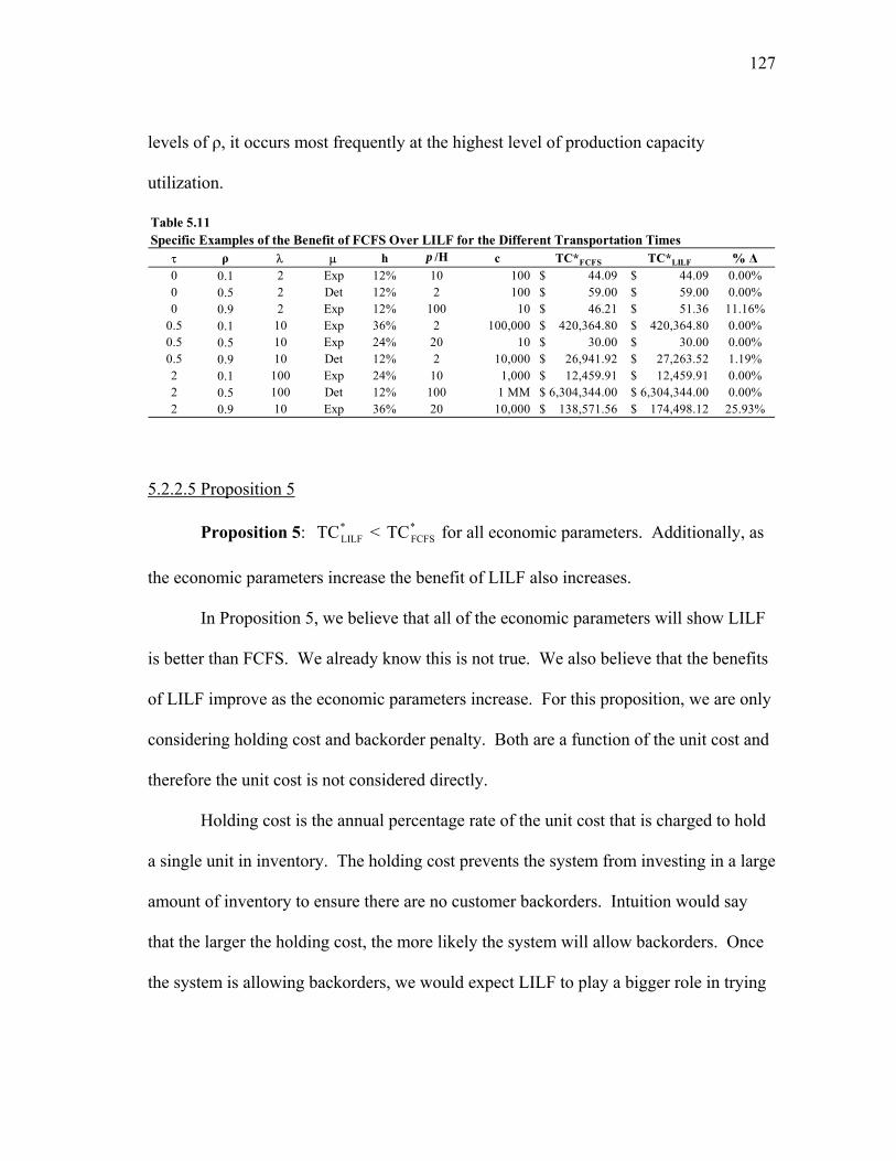
127

levels of ρ, it occurs most frequently at the highest level of production capacity

utilization.

Table 5.11Specific Examples of the Benefit of FCFS Over LILF for the Different Transportation Times

τ ρ λ µ h p /H c TC*FCFS TC*LILF % ∆0 0.1 2 Exp 12% 10 100 44.09$ 44.09$ 0.00%0 0.5 2 Det 12% 2 100 59.00$ 59.00$ 0.00%0 0.9 2 Exp 12% 100 10 46.21$ 51.36$ 11.16%

0.5 0.1 10 Exp 36% 2 100,000 420,364.80$ 420,364.80$ 0.00%0.5 0.5 10 Exp 24% 20 10 30.00$ 30.00$ 0.00%0.5 0.9 10 Det 12% 2 10,000 26,941.92$ 27,263.52$ 1.19%2 0.1 100 Exp 24% 10 1,000 12,459.91$ 12,459.91$ 0.00%2 0.5 100 Det 12% 100 1 MM 6,304,344.00$ 6,304,344.00$ 0.00%2 0.9 10 Exp 36% 20 10,000 138,571.56$ 174,498.12$ 25.93%

5.2.2.5 Proposition 5

Proposition 5: *LILFTC < *

FCFSTC for all economic parameters. Additionally, as

the economic parameters increase the benefit of LILF also increases.

In Proposition 5, we believe that all of the economic parameters will show LILF

is better than FCFS. We already know this is not true. We also believe that the benefits

of LILF improve as the economic parameters increase. For this proposition, we are only

considering holding cost and backorder penalty. Both are a function of the unit cost and

therefore the unit cost is not considered directly.

Holding cost is the annual percentage rate of the unit cost that is charged to hold

a single unit in inventory. The holding cost prevents the system from investing in a large

amount of inventory to ensure there are no customer backorders. Intuition would say

that the larger the holding cost, the more likely the system will allow backorders. Once

the system is allowing backorders, we would expect LILF to play a bigger role in trying

128

to reduce the number of backorders, especially under penalty policy p where a penalty is

paid regardless of how long the customer waits.

From the results, we see that holding cost has no effect on the impact of LILF on

the total inventory cost. Table 5.12 and Figure 5.9 show that for all levels of h LILF

wins almost exactly 35.7% (the overall percentage of LILF wins) of the time, under

penalty p. Under penaly π, the line is flat and LILF wins at the exact same rate (28.9%)

for every level of holding cost as the overall percentage of LILF wins. We conjecture

that holding cost impacts both LILF and FCFS equally and therefore it may affect the

base-stock policy equally for both order processing policies without affecting the

relationship between the policies.

Table 5.12LILF Wins by Holding Cost

h p π

28.9%

28.9%

28.9%35.4%

0.24 35.9%

0.36 35.9%

0.12

129

35.4% 35.9% 35.9%

28.9%28.9%28.9%

0.0%

20.0%

40.0%

0.12 0.24 0.36

Holding Cost

Percentage of LILF Wins

pπ

Figure 5.9. LILF Wins by Holding Cost

If holding cost is the constraint that prevents unlimited or large volumes of

inventory from building up, then the backorder penalty ratio is the constraint that keeps

the system from keeping no inventory and making every customer wait. Given the

results from the holding cost analysis, we would now expect to see the same pattern for

backorder penalty ratio as we did for holding cost. In Table 5.13 and Figure 5.10, we

find support for this new insight for the backorder penalty p. Backorder penalty π shows

a slightly different pattern.

130

Table 5.13LILF Wins by Penalty Ratio

B/H p π

100 34.1% 34.2%

36.9% 28.7%

36.0% 29.6%20

10

2 35.9% 23.1%

35.9% 36.9% 36.0%

34.1%

29.6%28.7%

23.1%

34.2%

0.0%

20.0%

40.0%

2 10 20 100

Backorder to Holding Cost Ratio

Percentage of LILF Wins

pπ

Figure 5.10. LILF Wins by Backorder to Holding Cost Ratio

In Table 5.13 and Figure 5.10, we see that the backorder penalty ratio, π/H, has

an increasing, positive effect on the impact of LILF on the total inventory cost. Under p,

the backorder penalty ratio had no effect on the impact of LILF. Recall, under p the

penalty was paid the moment the customer encountered a backorder. Therefore, there is

no difference if the customer waits for 1/100th of a time period or 20 time periods. In

131

either case the back order penalty is paid. However, under π there is a difference in the

time it the customer waits. As a result, we conjecture that reshuffling the queue affects

the amount of time a customer waits while in backorder and thereby lowers the amount

of penalty paid to the customer.

In terms of specific cases which show evidence that does not support the

propositions, we have already shown cases that do not support Proposition 5. In Table

5.14, we show that a single case in which *LILFTC > *

FCFSTC can also demonstrate that

*LILFTC can be greater than *

FCFSTC for all holding cost values and for all values of B/H,

which in this case is p/H. While increases in the holding costs show larger numerical

differences between the other cases holding all other parameters constant, the actual

percent difference between *LILFTC and *

FCFSTC remains the same. This is indicative of

the relationship between the holding costs and the inventory costs. As the holding cost

percentage increases, the total inventory cost increases because it is a function of the cost

to hold the necessary inventory to offset the cost of backordering.

Table 5.14 also shows that the optimal base-stock level for the case at hand does

not depend on the holding cost. The optimal base-stock level is a function of the back

order penalty to holding cost ratio, at least up to a point. The optimal base-stock level

increases equally for all three values of the holding cost. The increases can be seen

between the cases where p/H increases from 2 to 10 and then 10 to 20. From p/H = 20

to p/H = 100, neither the optimal base-stock level changes nor does the total inventory

cost of LILF or FCFS.

132

Table 5.14Specific Examples of the Benefit of FCFS Over LILF for the Different Economic Parameters

h p /H c BSLLILF BSLFCFS TC*LILF TC*FCFS TC*LILF - TC*FCFS % ∆12% 2 1,000 14 14 $ 1,245.01 $ 1,210.08 $ 34.93 2.89%12% 10 1,000 15 15 $ 1,435.09 $ 1,347.61 $ 87.48 6.49%12% 20 1,000 17 16 $ 1,499.93 $ 1,380.04 $ 119.89 8.69%12% 100 1,000 17 16 $ 1,499.93 $ 1,380.04 $ 119.89 8.69%24% 2 1,000 14 14 $ 2,490.02 $ 2,420.16 $ 69.86 2.89%24% 10 1,000 15 15 $ 2,870.18 $ 2,695.22 $ 174.96 6.49%24% 20 1,000 17 16 $ 2,999.86 $ 2,760.07 $ 239.78 8.69%24% 100 1,000 17 16 $ 2,999.86 $ 2,760.07 $ 239.78 8.69%36% 2 1,000 14 14 $ 3,735.04 $ 3,630.24 $ 104.80 2.89%36% 10 1,000 15 15 $ 4,305.28 $ 4,042.84 $ 262.44 6.49%36% 20 1,000 17 16 $ 4,499.78 $ 4,140.11 $ 359.68 8.69%36% 100 1,000 17 16 $ 4,499.78 $ 4,140.11 $ 359.68 8.69%

▪ ρ = 0.5, λ = 2, µ = exponential, τ = 2

To summarize the results for Propositions 1-5, we have found that the

relationships between the design parameters and the impact of LILF on total inventory

cost differ from factor to factor. Two factors, holding cost and backorder penalty ratio

do not affect the impact of LILF on total inventory cost. Production capacity utilization,

ρ, had an increasing, positive effect on the impact of LILF while transportation time, t,

had a decreasing, negative effect. Increases in production time randomness, going from

deterministic to exponential processing times, had a slightly increasing, positive effect as

well. The demand arrival rate, λ, had a unique affect on the impact of LILF. As λ

increased, LILF won more often. However, as λ continued to increase, the impact

diminished and was eventually lower than the impact started out at.

In the examples shown in this section, we find that the three parameters that tend

to confuse the issue most often are capacity utilization, demand arrival rate, and

transportation time. This demonstrates that predicting what is going to happen in a

modest three-stage supply chain is not so simple. We propose that trying to guess as to

what might happen in a much more complex real-world supply chain is next to

133

impossible. Therefore, we would counsel against using blanket statements about how

orders should be processed for any given supply chain design.

5.3 Cost Justification of the Zheng and Zipkin Cases

In their paper, Zheng and Zipkin (1990) presented results that indicated that the

real-time information policy of longest queue first was always superior to first-come,

first-serve policy. They also claimed that this would be the case regardless of the

economics imposed on the model. While the claim of relative superiority, using

equivalent parameters, was confirmed by our simulations, we are left wondering whether

or not the actual dollar amounts saved under these scenarios could justify the expense of

the real-time information system that would need to be implemented.

We looked at the annual cost savings under p and π for each of the cases that

represent the Zheng and Zipkin (1990) test cases. The greatest cost savings we could

find was when demand arrivals were equal to 100 per period, production utilization was

90%, transportation time was zero, annual holding cost was 36%, and the unit cost was

$1,000,000. The total inventory costs did not change with increases in p/H (this case

assumed the p penalty cost structure) because the optimal base-stock level occurred

when the PSO was zero. The difference in costs was $362,268 per year. While this

amount seems significant and could possibly justify the long-term investment in a small-

scale information system, we must question whether or not the assumptions are valid.

We do not believe that an industry exists where $1M units are being sold at a

constant rate of 100/day for an entire year. Even if transportation could be eliminated,

the volume for such an expensive product seems dubious. A company like GE, for

134

example, may sell jet engines at well over $1M/unit but they do not sell 36,500 of them a

year. Additionally, a company the size of Boeing would need to invest in an information

system to support their entire operation, which could never be paid for at a savings of

$362,268 a year. Most ERP systems cost several hundred million dollars for companies

the size of GE and Boeing (O’Leary, 2000). Therefore, it would be very difficult to

prove economic feasibility for purchasing a real-time information system based on the

change from FCFS to LILF.

5.4 Conclusions

The simulation results shed light on the debate for using real-time information to

alter the production schedule. First of all, we were able to show on the macro and micro

level that the results do not support the claim that LILF is always better than FCFS. We

were also able to find that production utilization, demand arrival rate, and deterministic

transportation time are the three design parameters that seem to drive the impact of LILF

on total inventory cost.

Of particular importance, we are able to see how the process parameters can

affect a company’s decision to use real-time information to reshuffle the production

queue. All else remaining equal, if a production facility has a high, steady capacity

utilization level, the firm would want to look into the benefits of using real-time

information. However, if that high utilization rate is coupled with longer transportation

time, the benefits of LILF may not materialize unless the way inventory level is

calculated changes.

135

Additionally, having a high demand arrival rate is not necessarily an indication

that the company should invest in a real-time information system, nor does having

random production times. In fact, if production times are random and demand arrival

rates are anything other than “mid-level,” the company may seriously want to consider

sticking with FCFS as an order processing policy.

Our results also quantify the cost savings between LILF and FCFS when LILF

does indeed provide them. The annual total cost savings in these cases are small and

could not justify the investment in a real-time information system. However, we do not

claim that LILF is the only other possible order processing strategy. There are other

potential processing strategies that may yield better results than LILF and prove

economically feasible to implement. This is another potential area for future research

consideration.

The goal of this research was not to find the optimal order processing policy. It

may very well be that the method we used to determine which order receives priority can

be dominated by several other methods. The goal of this research was to determine how

much better LILF is than FCFS and whether that relationship always holds. We believe

the pursuit of the optimal order processing policy will be long and difficult, providing

varied and interesting research possibilities.

136

CHAPTER VI

COMPARING FOUR-STAGE SUPPLY CHAIN DESIGNS

6.1 Constructing a Four-Stage Supply Chain Model

In the last chapter, we presented the results of using our three-stage ARB

simulator to determine whether or not cases exist where the FCFS order processing

policy fared better than the LILF order processing policy. In Chapter IV we presented

six propositions indicating our belief that LILF would always provide lower total

inventory costs than FCFS, based on the findings of Zheng and Zipkin (1990) and the

supporting findings of DeCroix and Arreola-Risa (1998). We were surprised to find

cases that did not support those propositions. Therefore, we decided to expand the ARB

capabilities to incorporate a second production stage, thus increasing the total number of

supply chain stages to four, in an effort to determine whether or not the restricted

number of stages influenced the effectiveness of LILF.

The four-stage supply chain simulator, ARB2, is an extension of ARB. The

runtime and model parameters remain the same for both simulators. The input

parameters and the input process outlined in Chapter III for ARB apply to ARB2 as well.

The addition of the second production stage required significant internal code changes,

but did not change the simulator’s interface, except to add additionally reporting options

for the second production stage. Therefore, the changes discussed in this section deal

strictly with the internal workings of the simulator to accommodate the second

production stage.

137

Figure 6.1 provides a graphical depiction of the four-stage supply chain model

implemented in ARB2. The addition of a second production stage is accompanied by

the addition of a second production queue. The second queue and production stage are

replicas of the first queue and production stage. However, the processing policy selected

for each simulation run is applied to the order queues independently. When the first

stage production machine is free, it looks to reshuffle the queue, or not depending on the

policy for the run, based on the current inventory levels of the distribution center –

product combinations. When the second stage production machine is available, it will

shuffle its queue independently of the first stage. The inputs and design parameters for

the first stage, however, apply to the second stage as well. While providing independent

parameters for both stages is both feasible and able to be implemented with relative ease,

the potential number of combinations would create a much more complex environment

to analyze. Therefore, we decided to implement an identical second stage in an effort to

simplify the effects the second stage would have on the results. Once these results are

analyzed, the potential for more research exists in this area by allowing the second stage

to have parameters independent of the first stage.

138

ProductionStage 2

Customer

X0X000XOrder Queue 1X0X000XOrder Queue 1

p1

p2

pn

DC 1

p1

p2

pn

p1

p2

pn

DC 1

p1

p2

pn

DC n

p1

p2

pn

p1

p2

pn

DC n

Customer

Figure 6.1: ARB Four-Stage Supply Chain Model

X0X000XOrder Queue 2X0X000XOrder Queue 2

ProductionStage 1

Fig. 6.1. ARB Four-Stage Supply Chain Model

The complexities involved with adding a second stage are two-fold. The first is

keeping track of the orders waiting in each queue and the statistics related to the orders

has they move through the second stage. The second complexity is that we are building

a queuing network instead of an M/M/1 queuing system. By creating an identical second

stage, we can minimize the complexity of the problem by building onto a system we

know works correctly.

We know how to keep track of the statistics of interest in the three-stage model

and transferring those techniques to the four-stage model are straightforward. From a

programming standpoint, the work is highly involved but low on the overall scale of

implementation complexity. The heart of the code for implementing the four-stage

supply chain model can be found in Appendix C. The full code can be obtained by

contacting the author.

139

6.2 Four-Stage Supply Chain Research Problem

To our knowledge, the analytical equivalent to test our four-stage supply chain

design problem, such as was done by Zheng and Zipkin (1990) for the three-stage

design, has never been performed. Therefore, we make no claims about comparing our

results to results presented in another study. Our propositions for this experiment are

based on the intuition and insight gathered from the three-stage problem in the previous

chapter.

As stated, this model consists of a second production queue and a second

production stage. It is the addition of this production queue that leads us to believe that

LILF may be able to provide greater help in a four-stage supply chain model over a

three-stage supply chain model. With a second opportunity to prioritize customer orders

based on need, we believe that LILF and the real-time information system behind it will

lead to bigger savings as compared to FCFS.

From the three-stage supply chain experiment, we learned that blanket statements

about LILF providing lower total inventory costs than FCFS under all conditions are not

supported by the data. We believe that the same premise holds true for the four-stage

model. Therefore, we believe comparing the four-stage output to the three-stage output

to be a more interesting case than directly comparing the four-stage LILF and FCFS

results. Accordingly, our propositions about the four-stage model will be based on

comparing it to the three-stage model results.

Due to the extra production queue, and thus a second opportunity for LILF to

contribute to lowering the total cost of inventory, we believe there will be a greater

140

number of cases in the four-stage model that show LILF providing a lower total

inventory cost than FCFS. Because both experiments will use the same number of cases,

we can look at the number of cases in percentage terms.

Proposition 1: The percentage of cases where LILF provides a lower total

inventory cost than FCFS in the three-stage model (P3) is less than the percentage of

cases in the four-stage model (P4). In equation terms, we believe P3 < P4.

In the three-stage model, we found that low utilization rates produced no

difference in total inventory costs between LILF and FCFS. We expect that pattern will

hold, or the number of cases that show a difference between the two order processing

policies will be very small. We also saw that the single biggest factor in the magnitude

of the difference *LILFTC - *

FCFSTC was the production utilization factor, ρ. Therefore,

we believe that LILF in the four-stage model will provide increasing benefits as ρ

increases. We also saw that the demand arrival rate (λ) had a unique effect on the

number of times LILF won. As demand arrivals increased from two per period to ten,

the percentage of LILF wins increased. However, as demand arrivals increased from ten

to one hundred, the percentage of LILF wins decreased. We would expect the same

pattern to hold for the four-stage model as well. However, under the four-stage model,

we expect the actual number of wins to be higher than in the three-stage model.

Proposition 2: As ρ increases, the difference P4 - P3 will increase.

Proposition 3: P4 - P3 > 0 for all λ.

Based on our first three propositions, it should be clear that we expect an increase

in help from the LILF policy in the four-stage model. Using the same logic, that there is

141

more opportunity for help in the four-stage model, we expect the gap between LILF and

FCFS to be greater in the four-stage model than in the three-stage model. That being

said, we can only compare the cases from the two models in which the difference

*LILFTC - *

FCFSTC < 0. This indicates that LILF has a lower TC* than FCFS. D3

represents the difference *LILFTC - *

FCFSTC for the three-stage model and D4 represents

the same difference for the four-stage model.

Proposition 4: D4 > D3 for all matching cases where D4 and D3 are negative.

The settings used in the three-stage model simulations will be used in the four-

stage model simulations. These settings are reviewed in the next section.

6.3 Experimental Design

The experimental design for investigating our three propositions require that we

run the four-stage model with the same parameter settings and do so for the same

combination of parameters. This will yield the same number of simulation runs

(15,552). For completeness, the parameters are provided in Table 6.1.

6.4 Experimental Results

Using the same parameters as the three-stage model, we ran 15,552 simulations.

The simulation runs took just over 150 hours. In order to compare the data to three-stage

model results, we first determined the difference *LILFTC - *

FCFSTC for both p and π. We

then classified the data according to the differences found at the aggregate level and then

by utilization levels. Finally, we determined the cases for which the difference *LILFTC -

*FCFSTC was less than zero, indicating that LILF provided a lower total cost of inventory.

142

We then extracted the cases in which the difference *LILFTC - *

FCFSTC was less than zero

for both the three-stage and four-stage models for comparison purposes. For these cases,

we calculated the number of cases in for which the four-stage model produced larger

*LILFTC - *

FCFSTC differences than the three-stage model. The results are shown below.

Table 6.1Four-Stage Design ParametersFixed Parameters ValuesDistribution Centers (i) 1Products (j) 2Product Type HomogeneousNumber of Machines (k) 1Run-Time (periods) 1,000,000Warm-up 10%

Variable Parameters ValuesDemand Arrival Rate (λ) 2; 10; 100

Production Time Distribution (µ) Deterministic; Exponential

Capacity Utilization (ρ) 0.1; 0.5; 0.9

Transportation Time (τ, in periods) 0; 0.5; 2.0

Unit Cost (c, in $) 10; 100; 1,000; 10,000; 100,000; 1MM

Annual Holding Cost (h) 12%; 24%; 36%

Backorder/Holding Cost Ratio (B/H) 2; 10; 20; 100

Backorder Penalties (p, π) p = $ / unit; π = $ /unit / unit time

Order Processing Rules LILF; FCFS

Proposition 1 stated that LILF would provide help in more cases for the four-

stage model than the three-stage model. The rationale is that there are two queues and

therefore greater opportunity to lower the total cost of inventory by reshuffling the

143

queues. Tables 6.2 and 6.3 show the differences between the two models for both p and

π, respectively. It is important to note, once again that the percentages listed in the

tables are derived by counting the number of wins for the order policies. Therefore, the

percentage of wins cannot be compared for statistical significance. To help the reader

make comparisons by row and column, the percentage of wins for both FCFS and LILF

have been included.

Table 6.2

Order Policy Three-Stage Four-Stage

FCFS 64.3% 77.3%

LILF 35.7% 22.7%

Overall Percentage of Wins by Model and Policy, Under Penalty p

Table 6.3

Order Policy Three-Stage Four-Stage

FCFS 71.1% 75.6%

LILF 28.9% 24.4%

Overall Percentage of Wins by Model and Policy, Under Penalty π

As in the previous chapter, we consider cases in which FCFS and LILF provide

the same total inventory cost as a “win” for FCFS because it is free to implement. For

these cases, the four-stage model has about 13% more cases under p and 4.5% more

cases under π where FCFS dominates LILF. In the three-stage model, FCFS dominates

64.3% of the time under p and 77.3% of the time under π. The percentage of wins for

FCFS in the three-stage model matches what was found in the previous chapter. We see

144

that LILF has a larger impact on the total inventory cost in the three-stage model than it

does in the four-stage model. Therefore, our results do not support Proposition 1.

Proposition 2 states that as ρ increases the percentage of cases in which LILF

dominates FCFS will increase linearly. This implies that the difference in cases at the

ρ=0.5 level will be greater than the ρ=0.1 level and ρ=0.9 level will be greater than the

ρ=0.5 level. Table 6.4 and Figure 6.2 present the results under penalty p. Table 6.5 and

Figure 6.3 present the results under penalty π.

Table 6.4

ρ Three-Stage Four-Stage ∆ % ∆

0.1 2.8% 2.8% 0.0% 0.0%

0.5 47.4% 41.6% -5.8% -12.2%

0.9 56.9% 23.6% -33.3% -58.5%

Percentage of LILF Wins by Model and Capacity Utilization Level Under Penalty p

Percentage of LILF Wins by Model and Capacity Utilization Level Under Penalty p

47.4%

23.6%

56.9%

2.8%

41.6%

0.0%

10.0%

20.0%

30.0%

40.0%

50.0%

60.0%

0.1 0.5 0.9

Capacity Utilization

Perc

enta

ge o

f LIL

F W

ins

Three-Stage

Four-Stage

Figure 6.2. Model Comparison by Capacity Utilization Under p

145

Table 6.5

ρ Three-Stage Four-Stage ∆ % ∆

0.1 2.0% 2.8% 0.7% 35.8%

0.5 38.8% 48.8% 10.0% 25.8%

0.9 45.8% 21.5% -24.3% -53.1%

Percentage of LILF Wins by Model and Capacity Utilization Level Under Penalty π

Percentage of LILF Wins by Model and Capacity Utilization Level Under Penalty π

21.5%

38.8%

2.0%

45.8%

2.8%

48.8%

0.0%

10.0%

20.0%

30.0%

40.0%

50.0%

60.0%

0.1 0.5 0.9

Capacity Utilization

Perc

enta

ge o

f LIL

F W

ins

Three-Stage

Four-Stage

Figure 6.3. Model Comparison by Capacity Utilization Under π

When looking at the percentage of LILF wins under p in Table 6.4, we see that

the proposed trend does not hold for the four-stage model. At the ρ = 0.5 level, the four-

stage model has fewer LILF dominate cases than the three-stage model by -5.8% and the

gap increases to -33.3% fewer cases at the ρ = 0.9 level. Therefore, the gap increases but

in the wrong direction. In actuality, what we expected to happen for LILF occurred for

FCFS. The ρ = 0.5 and ρ = 0.9 gaps increased in favor of FCFS by 4.5% and 33.3%,

146

respectively. In the case of penalty type π in Table 6.5, the dominance of LILF

increased at the ρ = 0.5 by 10% but dropped at the ρ = 0.9 level by -24.3%.

We see that the results for capacity utilization do not follow the same pattern in

the four-stage model as the results of the three-stage model. Instead of an increasing

number of wins for LILF, the four-stage model has an inverted “U” shaped function,

indicating that LILF wins the most at the mid-level utilization and falls off as utilization

increases or decreases. The results cannot support Proposition 2 and the reasons why

this may be happening defy our intuition.

Proposition 3 states that for all demand arrival rates, the percentage of LILF wins

will be higher in the four-stage model than in the three-stage model. In Tables 6.6 and

6.7, we see that this is only true when demand arrives at a rate of 100 per period, under

both penalty p and π. In the previous chapter, we saw that the percentage of LILF wins

with respect to demand arrival rate followed an inverted “U” shaped curve under penalty

p for the three-stage model. Figure 6.4 shows that in the four-stage model, the

percentage of LILF wins follows a “U” shaped curve; however, it is not inverted. The

rationale for this occurrence defies our intuition.

Table 6.6

λ Three-Stage Four-Stage ∆ % ∆

2 36.0% 24.6% -11.4% -31.7%

10 46.2% 15.6% -30.6% -66.2%

100 25.0% 27.8% 2.8% 11.2%

Percentage of LILF Wins by Model and Demand Arrival Rate Under Penalty p

147

Table 6.7

λ Three-Stage Four-Stage ∆ % ∆

2 36.1% 26.8% -9.3% -25.8%

10 26.3% 18.8% -7.6% -28.7%

100 24.3% 27.6% 3.3% 13.5%

Percentage of LILF Wins by Model and Demand Arrival Rate Under Penalty π

Percentage of LILF Wins by Model and Demanad Arrival Rate Under Penalty p

46.2%

36.0%

25.0%

27.8%24.6%

15.6%

0.0%

5.0%

10.0%

15.0%

20.0%

25.0%

30.0%

35.0%

40.0%

45.0%

50.0%

2 10 100

Demand Arrival Rate

Perc

enta

ge o

f LIL

F W

ins

Three-Stage

Four-Stage

Figure 6.4. Model Comparisons by Demand Arrival Rate Under p

Proposition 4 states that in the cases where both the three-stage and the four-

stage models show that LILF is the dominant order processing strategy, the four-stage

cases will provide a larger difference *LILFTC - *

FCFSTC . In order to show this, we

matched up each simulation run by design parameter settings and calculated the

difference *LILFTC - *

FCFSTC . Once the differences were calculated, we determined the

148

number of cases in which the difference was equal, the cases where the three-stage

model dominated, and the cases where the four-stage model dominated. This analysis

was performed for both the p and π backorder penalties. The results are shown in Table

6.8.

Table 6.8D4 - D3 Comparison

Result p π

D4 = D3 7.1% 0.1%

D4 < D3 71.7% 67.6%

D4 > D3 21.2% 32.3% From Table 6.8 we see that in the case of backorder penalty p, the three-stage

model had a greater improvement (LILF over FCFS) than the four-stage model 71.7% of

the time and 67.6% of the time in the case of π. These results show that the results do

not support Proposition 4 either.

6.5 Conclusions

We anticipated that the four-stage model would demonstrate the superiority of a

real-time information order-processing rule, such as LILF, due to the extra opportunity

of reshuffling a second queue. However, we discovered that the impact of LILF on the

four-stage model was lower than its impact on the three-stage model, both in terms of

the number of cases in which LILF performed better and the degree to which it

decreased total inventory costs. Further investigation is required to sort out the root

cause of the counter-intuitive results.

149

Intuition may lead us in two directions when trying to decipher why the results

are what they are. First of all, we can look at the second queue as an opportunity to

further improve the process, or we can consider it a second place to muddy the waters.

If may be possible that the first queue optimizes based on a current inventory level and

the second queue then reverses the order when it is time to look at inventory levels to

determine which product should be produced first. This constant back-and-forth may be

less beneficial than the alternative of leaving things alone.

Second, we can look and say that the products are homogeneous in every respect,

and therefore the system should help or hurt them both equally. By helping or hurting

them both equally, the process should sort itself out and by helping even occasionally the

total cost of inventory should prove to be smaller under LILF than FCFS. This is clearly

not the case.

From the start, we have not claimed that we are attempting to find the optimal

order scheduling policy. We are only trying to compare the results of the two policies

and determine the extent of help that a real-time information system using a LILF policy

could help the total system costs. Further research may lead us into trying to tweak the

LILF policy or develop an alternative policy that might help even more. One issue is

that the way our LILF policy reshuffles the queue may not be optimal given

deterministic transportation times. LILF does not account for orders already in the

pipeline to the distribution centers. This may cause LILF to be less effective when

transportation time is introduced into the system. However, it does not account for why

150

LILF consistently yields very small differences in the total inventory cost such that the

savings could not justify the cost of a real-time information system.

In the end, what we know is that even a few variables create a lot of counter-

intuitive optimal behavior in production scheduling systems. The bottom line is that it is

not so easy to tell what the impacts of a real-time information system will be in a very

simple system, much less a very complex supply chain such as those found in real

business operations. Our suggestion would be to make sure the company could justify

an ERP system on other factors besides the total inventory cost savings that are

anticipated due to real-time information. If the cost justification for investing in an ERP

system hinges on order processing efforts and inventory savings, we would recommend

a very detailed analysis of the core business and potential benefits before allocating the

type of funds required to pay for a real-time information system such as an ERP system.

151

CHAPTER VII

SUMMARY AND CONCLUSIONS

We developed a conceptual model for supply chain design using a novel

approach for analyzing the current body of SCM literature, built the ARB Simulator for

comparing supply chain designs, and demonstrated the difficulty of developing an order

processing policy which can consistently beat FCFS.

In developing the SCDCM, we found that many of the key design dimensions

identified in the SCM literature are intertwined with one another. This overlap between

design dimensions helps illuminate the complexity that exists when both trying to design

a supply chain and actively manage one as well. We found that a good supply chain

design will address strategic as well as operational and tactical supply chain issues. We

also found that the SCM literature tends to lag behind the current business needs of

supply chain design as demonstrated through the comparison of the SCDCM to the

pragmatic issues we have come across in industry.

Our SCDCM research provides four contributions to the academic community.

First of all, this research demonstrates the usefulness of a quantitative algorithm in

dealing with qualitative, unstructured data. Secondly, this research provides a

comparison of the text mining results with currently accepted frameworks used to teach

supply chain management to business students. Third, this research provides a

conceptual model for the supply chain design elements. Fourth, this research looks at

the pragmatic approach of supply chain design and demonstrates the inadequacies of the

152

current SCM models, including the SCDCM that was derived from current academic

research.

In the next phase of this dissertation, we examined the idea that real-time

information always provides a lower total inventory cost that using a first-come, first-

serve approach to processing production orders. We have presented ARB, our specially

designed simulator that allows us to collect specific statistics, such as lead-time demand,

which allow us to more closely examine the implications of different order processing

policies.

We found that the introduction of only a few different design parameters can

introduce enough complexity into the supply chain design to cloud the FCFS vs. real-

time information issue. In fact, we found that in the majority of our test cases, FCFS

beat LILF in terms of the difference in total inventory cost.

Of particular importance, we are able to see how the process parameters can

affect a company’s decision to use real-time information to reshuffle the production

queue. All else remaining equal, if a production facility has a high, steady capacity

utilization level, the firm would want to look into the benefits of using real-time

information. However, if that high utilization rate is coupled with longer transportation

time, the benefits of LILF may not materialize unless the way inventory level is

calculated changes.

Additionally, having a high demand arrival rate is not necessarily an indication

that the company should invest in a real-time information system, nor does having

random production times. In fact, if production times are random and demand arrival

153

rates are anything other than “mid-level,” the company may seriously want to consider

sticking with FCFS as an order processing policy.

From the tactical supply chain design research, we provide two contributions to

the academic community. First, we built ARB, which is a contribution in and of itself.

We have provided the heart of the code for both the three-stage and four-stage models in

Appendices B and C. The complete code can be obtained by contacting the author.

Second, we have demonstrated that real-time information systems do not always provide

the benefits that are promised. Although we do not claim that real-time information

systems, such as ERP, do not provide benefits to a company, we caution against using

their perceived benefits over a FCFS order processing system as financial justification to

implement one.

Supply chain design is a topic with a great deal of potential and research

possibilities. It is also a very complex topic that is difficult to work with at the macro

level. However, we have conveyed the importance of considering the various

dimensions of supply chain management when designing a supply chain in order to

maximize the benefits each partner in the chain can obtain. The benefits of a well-

designed and “well-oiled” supply chain can be tremendous to the same extent that the

impact of not having the right supply chain design for the intended market can be

disastrous. We hope that this research contributes to decide which is which.

154

REFERENCES

Amundson, S. D., 1998. Relationships between theory-driven empirical research in operations management and other disciplines. Journal of Operations Management 16, 341-359.

Anderson, E., Fine, C. and Parker, G., 2000. Upstream volatility in the supply chain: The machine tool industry as a case study. Production and Operations Management 9(3), 239-261.

Angell, L.C. and Klassen, R.D., 1999. Integrating environmental issues into the mainstream: An agenda for research in operations management. Journal of Operations Management 17(5), pp. 575-598.

Arreola-Risa, A., 1996. Integrated multi-item production-inventory systems. European Journal of Operational Research 89 (2), 326-340.

Arreola-Risa, A., 1998. On inventory abatement via manufacturing randomness reductions. Decision Sciences 29 (4), 983-1004.

Benton, W.C., Maloni, M., 2005. The influence of power driven buyer/seller relationships on supply chain satisfaction. Journal of Operations Management 23, 1-22.

Bertazzi, L., Speranza, M., 1999. Minimizing logistics costs in multistage supply chains. Naval Research Logistics 46, 399-417.

Bowen, F., Cousins, P., Lamming, R., Faruk, A., 2001. The role of supply management capabilities in green supply. Production and Operations Management 10 (2), 174-189.

Boyer, K.K. and Lewis, M.W., 2002. Competitive priorities: Investigating the need for trade-offs in operations strategy. Production and Operations Management 11 (1), 9-20.

Brickley, J.A., Smith, C.W., and Zimmerman, J.L., 2001. Managerial Economics and Organizational Architecture. McGraw-Hill, New York, NY.

Cachon, G.P., Lariviere, M.A., 2001. Contracting to assure supply: How to share demand forecasts in a supply chain. Management Science 47 (5), 629-646.

Chan, L.M.A., Muriel, A., Shen, Z., and Simchi-Levi, D., 2002. On the effectiveness of zero-inventory ordering policies for the economic lot-sizing model with a class of piecewise linear cost structures. Operations Research 50(6), 1058-1067.

155

Chen, F., Federgruen, A., and Zheng, Y., 2001. Near optimal pricing and replenishment strategies for a retail/distribution system. Operations Research 49(6), 839-853.

Chen, I.J., Paulraj, A., 2004. Towards a theory of supply chain management: The constructs and measurements. Journal of Operations Management 22, 119-150.

Chen, I., Paulraj, A., Lado, A., 2004. Strategic purchasing, supply management, and firm performance. Journal of Operations Management 22, 505-523.

Chen, F., Samroengraja, R., 2004. A staggered ordering policy for one-warehouse, multiretailer systems. Operations Research 52 (5), 707-722.

Chopra, S. and Meindl, P., 2004. Supply Chain Management: Strategy, Planning and Operations, 2nd Edition. Prentice Hall, Englewood Cliffs, NJ.

Christopher, M., 1998. Logistics and Supply Chain Management. Strategies for Reducing Cost and Improving Service, 2nd Edition. Prentice Hall, London.

Christopher, M. and Towill, D.R., 2002. Developing market specific supply chain strategies. International Journal of Logistics Management 13 (1), 1-14.

Clemen, R. T., 1996. Making hard decisions: An introduction to decision analysis, 2nd Edition. Duxbury Press, Belmont, California.

DeCroix, G.A., Arreola-Risa, A., 1998. Optimal production and inventory policy for multiple products under resource constraints. Management Science 44 (7), 950-961.

Eisenstein, D. and Iyer, A., 1996. Separating logistics flows in the Chicago public school system. Operations Research 44(2), 265-273.

Fan, W., Wallace, L., Rich, S., and Zhang, Z., 2006. Tapping the power of text mining. Communications of the ACM 49 (9), 77-82.

Ferguson, M. and Ketzenberg, M.E., 2006. Information sharing to improve retail product freshness of perishables. Production and Operations Management 15(1), 57-73.

Fine, C., 2000. Clockspeed-based strategies for supply chain design. Production and Operations Management 9(3), 213-221.

Fisher, M.L., 1997. What is the right supply chain for your product? Harvard Business Review March-April, 105-116.

Frazell, E., 2002. Supply Chain Strategy: The Logistics of Supply Chain Management. McGraw-Hill, New York, NY.

156

Gross, D. and Harris, C.M., 1985. Fundamentals of Queueing Theory. John Wiley & Sons, Inc, New York, NY.

Guide Jr., V.D.R., Jayaraman, V., Linton, J.D., 2003. Building contingency planning for closed-loop supply chains with product recovery. Journal of Operations Management 21, 259-279.

Guillen, G., Badell, M. and Puigjaner, L., 2007. A holistic framework for short-term supply chain management integrating production and corporate financial planning. International Journal of Production Economics 106, 288-306.

Gunasekaran, A., Ngai, E.W.T., 2004. Information systems in supply chain integration and management. European Journal of Operational Research 159 (2), 269-295.

Hadley, G. and Whitin, T.M., 1963. Analysis of Inventory Systems. Prentice Hall, Englewood Cliffs, NJ.

Hale, R., 2005. Editorial. Drug Discovery Today 10 (6), 377-379.

Handfield, R.B. and Melnyk, S.A., 1998. The scientific theory-building process: A primer using the case of TQM. Journal of Operations Management 16, 321-339.

Heizer, J. and Render, B., 2004. Operations Management, 7th Edition. Prentice Hall, Englewood Cliffs, NJ.

Heyman, D.P. and Sobel, M.J. eds., 1990. Handbooks in Operations Research and Management Science: Stochastic Models. Elsevier, New York, NY.

Huchzenmeir, A. and Cohen, M., 1996. Valuing operational flexibility under exchange rate risk. Operations Research 44(1), 100-113.

Johnson, M.E., Whang, S., 2002. E-business and supply chain management: An overview and framework. Production and Operations Management 11 (4), 413-423.

Johnson, R.A. and Wichern, D.W., 2007. Applied Multivariate Statistical Analysis, 6th Edition. Prentice Hall, Englewood Cliffs, NJ.

Juttner, U., Christopher, M. and Baker, S., 2007. Demand chain management-integrating marketing and supply chain management. Industrial Marketing Management 36, 377-392.

Kaminsky , P., Simchi-Levi, D., 2003. Production and distribution lot sizing in a two-stage supply chain. IIE Transactions 35, 1065-1075.

157

Ketzenberg, M.E., Rosenzweig, E.D., Maruchek, A.E., and Metters, R.D., 2007. A framework for the value of information in inventory replenishment. European Journal of Operational Research 182(3), 1230-1250.

Ketzenberg, M.E., van der Laan, E., and Teunter, R.H., 2006. Value of information in closed loop supply chains. Production and Operations Management 15(3), 393-406.

Kouvelis, P. and Milner, J.M., 2002. Supply chain capacity and outsourcing decisions: the dynamic interplay of demand and supply uncertainty. IIE Transactions 34(8), 717-728.

Krajewski, L. and Wei, J., 2001. The value of production schedule integration in supply chains. Decision Sciences 32(4), 601-634.

Lambert, D.M. and Knemeyer, A.M., 2004. We’re in this together. Harvard Business Review 82 (12), 114-122.

Law, A.M. and Kelton, W.D., 2000. Simulation Modeling and Analysis, 3rd Ed. McGraw-Hill, Boston, MA.

Lawton, C., 2006. Desk job: Consumer demand and growth in laptops leave dell behind. Wall Street Journal (Eastern Edition), New York, NY, A1.

Lee, H.L., 2002. Aligning supply chain strategies with product uncertainties. California Management Review 44 (3), 105-119.

Lee, H.L., 2004. The triple a supply chain. Harvard Business Review October, 102-112.

Lee, H.L., Pabmanabhan, V., and Whang, S., 1997. Information distortion in the supply chain: The bullwhip effect. Management Science 43(4), 546-558.

Lee, H.L. and Whang, S., 2001. Demand chain excellence. Supply Chain Management Review March/April, 40-46.

Li, L., 2002. Information sharing in a supply chain with horizontal competition. Management Science 48 (9), 1196-1212.

Li, Q. and Wu, Y.B., 2006. Identifying important concepts from medical documents. Journal of Biomedical Informatics 39, 668-679.

Mabert, V.A., Venkataramanan, M.A., 1998. Special research focus on supply chain linkages: Challenges for design and management in the 21st century. Decision Sciences 29 (3), 537-552.

Meredith, J., 1993. Theory building through conceptual models. International Journal of Operations and Production Management 13 (5), 3-11.

158

Milner, J.M., Rosenblatt, M.J., 2002. Flexible supply contracts for short life-cycle goods: the buyer's perspective. Naval Research Logistics 49, 25-45.

Morash, E.A., 2001. Supply chain strategies, capabilities, and performance. Transportation Journal Fall, 37-54.

Narayanan, V.G and Raman, A., 2004. Aligning incentives in supply chains. Harvard Business Review November, 94-102.

O’Leary, D.E., 2000. Enterprise resource planning systems: Systems, life cycle, electronic commerce and risk. Cambridge University Press, New York, NY.

Porter, M.E., 1985. Competitive Advantage. Free Press, New York, NY.

Poulin, M., Montreuil, B. and Martel, A., 2006. Implications of personalization offers on demand and supply network design: A case from the golf club industry. European Journal of Operations Research 169, 996-1009.

Prahinski, C., Benton, W., 2004. Supplier evaluations: Communication strategies to improve supplier performance. Journal of Operations Management 22, 39-62.

Sahin, F., Robinson, E.P., 2002. Flow coordination and information sharing in supply chains: Review, implications and directions for future research. Decision Sciences 33 (4), 505-536.

Sanders, A. and DeVault, C., 2004. Using SAS at SAS: The mining of SAS technical support. International Conference SUGI-29 (Canada). Paper 010-29: Analytics Track.

SAS Institute, Inc., 2003. Text Mining Using SAS Software Course Notes. SAS Institute, Cary, NC.

SAS Institute, Inc., 2003. SAS Software Version 9.1 Help Files. SAS Institute, Cary, NC.

Schmenner, R. W. and Swink, M. L., 1998. On theory in operations management. Journal of Operations Management 17 (1), 97–113.

Simchi-Levi, D., Kaminsky, P. and Simchi-Levi, E., 2000. Designing and Managing the Supply Chain: Concepts, Strategies, and Cases. McGraw-Hill/Irwin, New York, NY.

Singh, N., Hu, C. and Roehl, W.S., 2007. Text mining a decade of progress in hospitality human resource management research: identifying emerging thematic development. International Journal of Hospitality Management 26(1), 131-147.

159

Sobel, M. and Zhang, R., 2001. Inventory policies for systems with stochastic and deterministic demand. Operations Research 49(1), 157-162.

Stadtler, H., 2005. Supply chain management and advanced planning--basics, overview and challenges. European Journal of Operational Research 163, 575-588.

Stanley, L., Wisner, J., 2001. Service quality along the supply chain: implications for purchasing. Journal of Operations Management 19, 287-306.

Subramani, M., 2004. How do suppliers benefit form information technology use in supply chain relationships? MIS Quarterly 28 (1), 45-73.

Swamidass, P.M., 1990. Empirical science: The new frontier in operations management research. Academy of Management Review 16 (4), 793-814.

Swaminathan, J.M., Tayur, S.R., 2003. Models for supply chain in e-business. Management Science 49 (10), 1387-1406.

Swanson, D.R. and Smalheiser, N.R., 1997. An interactive system for finding complementary literatures: A stimulus to scientific discovery. Artificial Intelligence 91, 183-203.

Techmistocleous, M., Irani, Z., Love, P., 2004. Evaluating the integration of supply chain information systems: A case study. European Journal of Operational Research 159, 393-405.

Thomas, D.J., Griffin, P.M., 1996. Coordinated supply chain management. European Journal of Operational Research 94, 1-15.

Thomas, M. and Mackey, J., 2006. Supply chain management: Monitoring strategic partnering contracts with activity-based measures. Management Accounting Quarterly 8 (1), 1-10.

Turban, E. and Meredith, J.K., 1991. Fundamentals of Management Science, 5th ed. Irwin, Homewood, IL.

Vasilis, T., Voss, C., Hadjinicola, G., and Soteriou, A., In Press. Insights on factors affecting production and operations management (POM) journal evaluations. Production and Operations Management.

Walters, D. and Rainbird, M., 2004. The demand chain as an integral component of the value chain. Journal of Consumer Marketing 21 (7), 465-475.

Warburton, R., 2007. An optimal, potentially automatable ordering policy. International Journal of Production Economics 107, 483-495.

160

Whitt, W., 1989. Planning queueing simulations. Management Science 35(11), p 1341-1366.

Whitt, W., 1991. The efficiency of one long run versus independent replication in steady-state simulation. Management Science 37(6), p 645-666.

Winston, W.L., 2004. Introduction to Probability Models, Operations Research: Volume Two, 4th Edition. Brooks/Cole, Toronto, Canada.

Yetisgen-Yildiz, M. and Pratt, W., 2006. Using statistical and knowledge-based approaches for literature-based discovery. Journal of Biomedical Informatics 39, 600-611.

Zaltnian, G., Lemasters, K. and Heffring, M., 1982. Theory Construction in Marketing: Some Thoughts on Thinking. Wiley, New York. NY.

Zheng, Y. and Zipkin, P., 1990. A queueing model to analyze the value of centralized inventory information. Operations Research 38 (2), 296-307.

Zipkin, P.H., 2000. Foundations of Inventory Management. McGraw-Hill, New York, NY.

Zhu, Q. and Sarkis, J., 2004. Relationships between operational practices and performance among early adopters of green supply chain management practices in Chinese manufacturing enterprises. Journal of Operations Management 22(3), 265-289.

161

APPENDIX A

Adelman, D., 2004. A price-directed approach to stochastic inventory/routing. Operations Research 52 (4), 499-514.

Agrawal, N., Cohen, M., 2001. Optimal Material Control in an Assembly System with Component Commonality. Naval Research Logistics 48, 409-429.

Agrawal, V., Seshadri, S., 2000. Risk intermediation in supply chains. IIE Transactions 32 (9), 819-831 .

Akkermans, H., Bogerd, P., Yucesan, E., Van Wassenhove, L., 2003. The impact of ERP on supply chain management: Exploratory findings from a European Delphi study. European Journal of Operational Research 146, 284-301.

Akkermans, H., Vos, B., 2003. Amplification In Service Supply Chains: An Exploration Case Study From The Telecom Industry. Production and Operations Management 12 (2), 204-223.

Alptekinoglu, A.., Tang, S., 2005. A model for analyzing multi-channel distribution systems. European Journal of Operational Research 163, 802-824.

Angell, L., Klassen, R., 1999. Integrating environmental issues into the mainstream: an agenda for research in operations management. Journal of Operations Management 17, 575-598.

Aviv, Y., 2001. The effect of collaborative forecasting on supply chain performance. Management Science 47 (10), 1326-1343.

Aviv, Y., 2003. A Time Series Framework for Supply Chain Inventory Management. Operations Research 51 (2), 210-227.

Axsanter, S., 2000. Exact analysis of continuous review (R,Q) policies in two-echelon inventory systems with compound poisson demand. Operations Research 48 (5), 686-696.

Axsater, S., Zhang, W., 1996. Recursive evaluation of order-up-to-S political for tow-echelon inventory systems with compound Poisson demand. Naval Research Logistics 43 (1), 151-157.

Ayanso, A., Diaby, M., Nair, S., 2004. Inventory rationing via drop-shipping in Internet retailing: A sensitivity analysis. European Journal of Operational Research 171, 135-152.

Bendiksen, B., Dreyer, B., 2003. Technological changes––the impact on the raw material flow and production. European Journal of Operational Research 144, 237-246.

Benton, W.C., Maloni, M., 2005. The Influence Of Power Driven Buyer/Seller Relationships On Supply Chain Satisfaction. Journal of Operations Management 23, 1-22.

162

Bernstein, F., Federgruen, A., 2003. Pricing And Replenishment Strategies In A Distribution System With Competing Retailers. Operations Research 51 (3), 409-426.

Bertazzi, L., Speranza, M., 1999. Minimizing Logistics Costs in Multistage Supply Chains. Naval Research Logistics 46, 399-417.

Bertsimas, D., Gamarnik, D., Sethuraman, J., 2003. From Fluid Relaxations to Practical Algorithms for High-Multiplicity Job-Shop Scheduling: The Holding Cost Objective. Operations Research 51 (5), 798-813.

Bhaskaran, S., 1998. Simulation analysis of a manufacturing supply chain. Decision Sciences 29 (3), 633-657.

Bhattacharjee, S., Ramesh, R., 2000. A multi-period maximizing model for retail supply chain management: an integrationof demand and supply-side mechanisms. European Journal of Operational Research 122 (3), 584-601.

Bookbinder, J., Cakanyildirim, M.A.., 1999. Random lead times and expedited orders in (Q, r) inventory systems. European Journal of Operational Research 115, 300-313.

Bordley, R., Kirkwood, C., 2004. Multiattribute Preference Analysis with Performance Targets. Operations Research 52 (6), 823-835.

Bowen, F., Cousins, P., Lamming, R., Faruk, A., 2001. The Role of Supply Management Capabilities in Green Supply. Production and Operations Management 10 (2), 174-189.

Bradley, J., Arntzen, B., 1999. The simultaneous Planning of Production, Capacity and Inventory in Seasonal Demand Environments. Operations Research 47 (6), 795-806.

Cachon, G., 1999. Managing supply chain demand variability with scheduled ordering policies. Management Science 45 (6), 843-856.

Cachon, G., Fisher, M., 2000. Supply Chain Inventory Management and the Value of Shared Information. Management Science 46 (8), 1032-1048.

Cachon, G., Lariviere, M., 1999. An equilibrium analysis of linear, proportional and uniform allocation of scarce capacity. IIE Transactions 31, 835-849.

Cachon, G.P., 2001. Stock Wars: Inventory Competition In A Two-Echelon Supply Chain With Multiple Retailers. Operations Research 49 (5), 658-674.

Cachon, G.P., Fisher, M., 1997. Campbell Soup'S Continuous Replenishment Program: Evaluation And Enhanced Inventory Decision Rules. Production and Operations Management 6 (3), 266-276.

Cachon, G.P., Lariviere, M.A., 2001. Contracting To Assure Supply: How To Share Demand Forecasts In A Supply Chain. Management Science 47 (5), 629-646.

163

Carlsson, D., Ronnqvist, M., 2005. Supply Chain Management In Forestry--Case Studies At Sodra Cell Ab. European Journal of Operational Research 163, 589-616.

Carter, C.R., 2000. Ethical issues in international buyer–supplier relationships: a dyadic examination. Journal of Operations Management 18, 191-208.

Centinkaya, S., Lee, C., 2002. Optimal outbound dispatch policies: Modeling inventory and cargo capacity. Naval Research Logistics 49 (6), 531-556.

Chan, L., Muriel, A., Shen, Z., Simchi-Levi, D., 2002. On the effectiveness of zero-invetory-ordering policies for the economic lot-sizing model with a class of piecewise linear cost structures. Operations Research 50 (6), 1058-1067.

Chandra, C., Grabis, J., 2005. Application of multi-steps forecasting for restraining the bullwhip effect and improving inventory performance under autoregressive demand. European Journal of Operational Research 166, 337-350.

Chang, Y., Lee, C., 2004. Machine scheduling with job delivery coordination. European Journal of Operational Research 158, 470-487.

Chen, B., Munson, C., 2001. Resource allocation with lumpy demand: to speed up or not to speed?. Naval Research Logistics 51 (3), 363-385.

Chen, F., 1999. Decentralized Supply Chains Subject To Information Delays. Management Science 45 (8), 1076-1090.

Chen, F., Ryan, J., Simchi-Levi, D., 2000. The impact of exponential emoothing forecasts on the bullwhip effect. Naval Research Logistics 47 (4), 269-286.

Chen, F., Samroengraja, R., 2000. Order Volatility And Supply Chain Costs. Operations Research 48 (2), 281-293.

Chen, F., Samroengraja, R., 2004. A Staggered Ordering Policy For One-Warehouse, Multiretailer Systems. Operations Research 52 (5), 707-722.

Chen, F., Song, J., 2001. Optimal polices for multi-echelon inventory problems with markovmodulated demand. Operations Research 49 (2), 226-234.

Chen, I., Paulraj, A., Lado, A., 2004. Strategic purchasing, supply management, and firm performance. Journal of Operations Management 22, 505-523.

Chen, I.J., Paulraj, A., 2004. Towards A Theory Of Supply Chain Management: The Constructs And Measurements. Journal of Operations Management 22, 119-150.

Cheung, K., Lee, H., 2004. The inventory benefit of shipment coordination and stock rebalancing in a supply chain. Management Science 50 (4), 445-457.

Cheung, K., Zhang, A., 1999. The impact of inventory information distortion due to customer order cancellations. Naval Research Logistics 46 (2), 213-231.

Chiang, W., Chhajed, D., Hess, J., 2003. Direct marketing, indirect profits: a strategic analysis of dual channel supply chain design. Management Science 49 (1), 1-20.

164

Chiang, W., Monahan, G., 2005. Managing inventories in a two-echelon dual-channel supply chain. European Journal of Operational Research 162, 325-341.

Choi, K., Dai, J., Song, J., 2000. On measuring supplier performance under vendor-managed-inventory programs in capacitated supply chains. Manufacturing & Service Operations Management 9 (3), 213-221.

Choi, T., Dooley, K., Rungtusanatham, M., 2001. Supply networks and complex adaptive systems: control versus emergence. Journal of Operations Management 19, 351-366.

Choi, T., Li, D., Yan, H., 2004. Quick Response Policy With Bayesian Information Updates. European Journal of Operational Research, In Press.

Chopra, S., Rao, M., Tsai, C., 1997. Computational Study of the Multiechelon Production Planning Problem. Naval Research Logistics 44, 1-19.

Chung, C., Flynn, J., Stalinski, P., 2001. A single-period inventory placement for a serial supply chain. Naval Research Logistics 48 (6), 506-517.

Chung, C., Hum, S., Kirca, O., 2000. An Optimal Procedure for the Coordinated Replenishment Dynamic Lot-Sizing Problem with Quantity Discounts. Naval Research Logistics 47, 686-695.

Cohen, M., Mallic, S., 1997. Global supply chain: Research and applications. Production and Operations Management 6 (3), 193-210.

Corbett, C., 2001. Sochastic Inventory Systems in a Supply Chain with Asymmetric Information: Cycle Stocks, Safety Stocks, and Consignment Stock. Operations Research 49 (4), 487-500.

Corbett, C., DeCroix, G., Hameri, A., 2005. Optimal shared-savings contract in supply chains: linear contracts and double moral hazards. European Journal of Operational Research 163 (3), 653-667.

Crama, Y., Pascual, P., Torres, A., 2004. Optimal procurement decisions in the presence of total quantity discounts and alternative product recipes. European Journal of Operational Research 159, 364-378.

Crespo, A., Bianchi, C., Gupta, J., 2004. Operational and Financial effectiveness of e-collaboration tools in supply chain integration. European Journal of Operational Research 159, 348-363.

Croson, R., Donohue, K., 2003. Impact of POS data sharing on supply chain management: An experimental study. Production and Operations Management 12 (1), .

Cvsa, V., Gilbert, S., 2002. Strategic commitment vs. postponement in a two-tier supply chain. European Journal of Operational Research 141, 526-543.

Daganzo, C., 2004. On the Stability of Supply Chains. Operations Research 52, 909-921.

165

Dasci, A., Verter, V., 2001. A continuous model for production-distribution system design. European Journal of Operational Research 129, 287-298.

Deshapande, V., Cohen, M., Donohue, K., 2003. An Empirical Study of Service Differentiation for Weapon System Service Parts. Operations Research 51 (4), 518-530.

Dogan, K., Goetschalckx, M., 1999. A Primal Decomposition Method For The Integrated Design Of Multi-Period Production-Distribution Systems. IIE Transactions 31 (11), 1027-1036.

Dong, Y., Carter, C., Dresner, M., 2001. JIT purchasing and performance: an exploratory analysis of buyer and supplier perspectives. Journal of Operations Management 19, 471-483.

Erhun, F., Tayur, S., 2003. Enterprise-wide optimization of total landed cost at a grocery retailer. Operations Research 51 (3), 343-353.

Ertek, G., Griffin, P.M., 2002. Supplier- And Buyer-Driven Channels in A Two-Stage Supply Chain. IIE Transactions 34 (8), 691-700.

Ertogral, K., Wu, S., 2000. Auction-theoretic coordination of production planning in the supply chain. IIE Transactions 32, 931-940.

Escudero, L., Galindo, E., Garcia, G., Gomez, E., Sabau, V., 1999. Schuman, a modeling framework for supply chain management under uncertainty. European Journal of Operational Research 119, 14-34.

Ettl, M., Feigin, G., Linton, G., Yao, D., 2000. A supply network model with base-stock control and service requirements. Operations Research 48 (2), 216-232.

Ferguson, M., 2003. When to Commit in a Serial Supply Chain with Forecast Updating. Naval Research Logistics 50, 917-936.

Frederix, F., 2001. An extended enterprise planning methodology for the discrete manufacturing industry. European Journal of Operational Research 129, 317-325.

Fricker, R., Goodhart, C., 2000. Applying a Bootstrap Approach for Setting Reorder Points in Military Supply Systems. Naval Research Logistics 47, 459-478.

Frohlich, M., 2002. e-Integration in the supply chain: barriers and performance. Decision Sciences 33 (4), 537-556.

Frohlich, M., Westbrook, R., 2001. Arcs of Integration: an international study of supply chain strategies. Journal of Operations Management 19, 185-200.

Gallego, G., Toktay, L., 2004. All-or-nothing ordering under a capacity constraint. Operations Research 52 (6), 1001-1002.

Gan, X., Sethi, S., Yan, H., 2004. Coordination of Supply Chains with risk-averse agents. Production and Operations Management 13 (2), 135-149.

166

Gans, N., Zhou, Y., 2003. A call-routing problem with service- level constraints. Operations Research 51 (2), 255-271.

Garg, A., 1999. An application of designing products and processes for supply chain management. IIE Transactions 31 (5), 417-429.

Garg, D., Narahari, Y., Viswanadham, N., 2004. Achieving sharp deliveries in supply chains through variance pool allocation. European Journal of Operational Research 171, 227-254.

Gavirneni, S., 2001. Benefits Of Co-Operation In A Production Distribution Environment. European Journal of Operational Research 130, 612-622.

Gavirneni, S., 2002. Information flows in capacitated supply chains with fixed ordering costs. Management Science 48 (5), 644.

Gavirneni, S., Kapuscinski, R., Tayur, S., 1999. Value of Information in Capacitated Supply Chains. Management Science 45 (1), 16-24.

Gavirneni, S., Tayur, S., 2001. An efficient procedure for non-stationary inventory control. IIE Transactions 33, 83-89.

Gerchak, Y., 2000. On the allocation of uncertainty-reduction effort to minimize total variability. IIE Transactions 32 (4), 403-407.

Geunes, J., Zeng, S., 2001. , Impacts of inventory shortage policies on transportation requirements in two-stage distribution systems. European Journal of Operational Research 129, 299-310.

Gigler, J., Hendrix, E., Heesen, R., Van den Hazelkamp, V., Meerdink, G., , 2002. On optimization of agri chains by dynamic programming. European Journal of Operational Research 139, 613-625.

Grover, V., Malhotra, M., 2003. Transaction cost framework in operations and supply chain management research: theory and measurement. Journal of Operations Management 21, 457-473.

Guide Jr., V.D.R., Jayaraman, V., Linton, J.D., 2003. Building Contingency Planning For Closed-Loop Supply Chains With Product Recovery. Journal of Operations Management 21, 259-279.

Gunasekaran, A., Ngai, E.W.T., 2004. Information Systems In Supply Chain Integration And Management. European Journal of Operational Research 159, 269-295.

Gunnarsson, H., Ronnqvist, M., Lundgren, J.T., 2004. Supply Chain Modeling Of Forest Fuel. European Journal of Operational Research 158, 103-123.

Ha, A., 2001. Supplier-buyer contracting: asymmetric cost information and cutoff level policy for buyer participation. Naval Research Logistics 48 (1), 41-64.

Hall, N., Potts, C., 2003. Supply chain scheduling: batching and delivery. Operations Research 51 (4), 566.

167

Hariga, M., 1998. A Single-Period, Multi-Echelon Stochastic Model Under A Mix Assembly To Order And Assemble In Advance Policies. Naval Research Logistics 45, 599-614.

He, Q., Jewkes, E., 2000. Performance measures of a make-to-order inventory-production system. IIE Transactions 32, 409-419.

Heese, H., Cattani, K., Ferrer, G., Gilland, W., Roth, A., , 2005. Competitive advantage through take-back of used products. European Journal of Operational Research 164, 143-157.

Heikkilä, J., 2002. From supply to demand chain management: efficiency and customer satisfaction. Journal of Operations Management 20, 747-767.

Hendricks, K., Singhal, V., 2003. The effect of supply chain glitches on shareholder wealth. Journal of Operations Management 21, 501-522.

Herer, Y., Tzur, M., 2001. The Dynamic Transshipment Problem. Naval Research Logistics 48, 386-408.

Herer, Y.T., Rashit, A., 1999. Lateral Stock Transshipments In A Two-Location Inventory System With Fixed And Joint Replenishment Costs. Naval Research Logistics 46, 525-547.

Hill, C., Scudder, G., 2002. The use of electronic data interchange for supply chain coordination in the food industry. Journal of Operations Management 20, 375-387.

Hillier, M., 1999. Product Commonality in Multiple-Period, Make-to-Stock Systems. Naval Research Logistics 46, 737- 751.

Huang, W., Kulkarni, V., Swaminathan, J., 2003. Optimal EOQ for announced price increase in infinite horizon. Operations Research 51 (2), 336.

Jammernegg, W., Kischka, P., 2005. Dynamic, customer oriented improvement of supply networks. European Journal of Operational Research 106, 413-426.

Jayaraman, V., Pirkul, H., 2001. Planning and coordination of production and distribution facilities for multiple commodities. European Journal of Operational Research 133, 394-408.

Johnson, M.E., Whang, S., 2002. E-Business And Supply Chain Management: An Overview And Framework. Production and Operations Management 11 (4), 413-423.

Johnson, P., Klassen, R., Leenders, M., Fearon, H., 2002. Determinants of purchasing team usage in the supply chain. Journal of Operations Management 20, 77-89.

Kachani, S., Perakis, G., 2006. Fluid dynamics models and their applications in transportation pricing. European Journal of Operational Research 170, 496-517.

168

Kaminsky , P., Simchi-Levi, D., 2003. Production and Distribution Lot Sizing in a Two Stage Supply Chain. IIE Transactions 35, 1065-1075.

Karaesmen, F., Buzacott, J., Dallery, Y., 2002. Integrating advance order information in make-to-stock production systems. IIE Transactions 34, 649-662.

Khouja, M., 2000. The economic lot and delivery scheduling problem: common cycle, rework, and variable production rate. IIE Transactions 32, 715-725.

Kim, B., 2000. Coordinating an Innovation in Supply Chain Management. European Journal of Operational Research 123, 568-584.

Kim, B., Leung, J.M.Y., Park, K.T., Zhang, G., Lee, S., , 2002. Configuring a Manufacturing Firm's Supply Network with Multiple Suppliers. IIE Transactions 34, 663-667.

Kim, H., Ryan, J., 2001. The cost impact of using forecasting techniques in a supply chain. Naval Research Logistics 50 (5), 388-411.

Klastorin, T., Moinzadeh, K., Son, J., 2002. Coordinating orders in supply chains through price discounts. IIE Transactions 34, 679-689.

Koksalan, M., Plante, R., 2003. Interactive Multi-criteria Optimization for Multiple-Response Product and Process Design. Manufacturing & Service Operations Management 5 (4), 334-347.

Kouvelis, P., Milner, J., 2002. Supply chain capacity and outsourcing decisions: the dynamic interplay of demand and supply uncertainty. IIE Transactions 34 (8), 717-728.

Krajewski, L., Wei, J., Tang, L., 2004. Responding to schedule changes in build-to-order supply chains. Journal of Operations Management, .

Krause, D., Handfield, R., Scannell, T., 1998. An empirical investigation of supplier development: reactive and strategic process. Journal of Operations Management 17, 39-58.

Krause, D., Pagell, M., Curkovic, S., 2001. Toward a measure of competitive priorities for purchasing. Journal of Operations Management 19, 497-512.

Kreipl, S., Pinedo, M., 2004. Planning and scheduling in supply chains: an overview of issues in practice. 13 (1), 77-92.

Kulp, S., Lee, H., Ofek, E., 2004. Manufacturers benefits from information integration with retail customers. Management Science 50 (4), 431-444.

Lawson, D.G., Porteous, E.L., 2000. Multistage Inventory Management with Expediting. Operations Research 48 (6), 878-893.

Lee, C., 2001. Coordinated stocking, clearance sales, and return policies for a supply chain. European Journal of Operational Research 131 (3), 491-513.

169

Lee, C., Chu, W., 2005. Who should control inventory in a supply chain?. European Journal of Operational Research 164 (1), 158-172.

Lee, C., Tan, S., Yan, H., 2003. Designing an Assembly Process with Stochastic Material Arrivals. IIE Transactions 35, 803-815.

Lee, H., So, K., Tang, C., 2000. The value of information sharing in a two-level supply chain. Management Science 46 (5), 626.

Lejeune, M., Yakova, N., 2005. On characterizing the 4 C's in supply chain management. Journal of Operations Management 23 (1), 81-100.

Li, C., Xiao, W., 2004. Lot streaming with supplier-Manufacturer Coordination. Naval Research Logistics 51 (4), 522-542.

Li, L., 2002. Information Sharing in a Supply Chain with Horizontal Competition. Management Science 48 (9), 1196-1212.

Li, L., Zhang, H., 2000. The Mulitstage Service Facility Start-up and Capacity Model. Operations Research 48 (3), 490-497.

Lu, Y., Song, J., Yao, D.D., 2003. Order Fill Rate, Lead-time Variability, and Advance Demand Information in an Assemble to Order System. Operations Research 51 (2), 292-308.

Mabert, V.A., Venkataramanan, M.A.., 1998. Special Research Focus on Supply Chain Linkages: Challenges for Design and Managmet in the 21st Century. Decision Sciences 29 (3), 537-552.

Mallik, S., Harker, P., 2004. Coordinating supply chains with competition: capacity allocation in semiconductor manufacturing. European Journal of Operational Research 159 (2), 330-347.

Marasimhan, R., Jayaraman, J., 1998. Casual linkages in supply chain management: an exploratory study of North American manufacturing firms. Decision Sciences 29 (3), 579-605.

Marklund, J., 2002. Centralized inventory control in a tow-level distribution system with Poisson demand. Naval Research Logistics 49 (8), 798-822.

Melachrinoudis, E., Min, H., 2000. The dynamic relocation and phase-out of a hybrid, two echelon plant/warehousing facility: A multiple objective approach. European Journal of Operational Research 123, 1-15.

Milner, J.M., Rosenblatt, M.J., 2002. Flexible Supply Contracts for Short Life-Cycle Goods: The Buyer's Perspective. Naval Research Logistics 49, 25-45.

Mishra, B., Raghunatahn, S., 2003. Retailer – vs. Vendor –Managed Inventory and Brand Competition. Management Science 50, 917-936.

Moinzadeh, K., Nahmias, S., 2000. Adjustment strategies for a fixed delivery contract. Operations Research 48 (3), 408-423.

170

Monizadeh, K., 2002. A multi-echelon inventory system with information exchange. Management Science 48 (3), 414.

Moses, M., Seshadri, S., 2000. Policy mechanisms for supply chain coordination. IIE Transactions 32 (3), 245-262.

Munson, C., Rosenblatt, M., 2001. Coordinating a three-level supply chain with quantity discounts. IIE Transactions 33 (5), 371-384.

Nagurney, A., Cruz, J., Dong, J., Zhang, D., 2005. Supply chain networks, electronic commerce, and supply side and demand side risk. European Journal of Operational Research 164, 120-142.

Nielsen, C., Larsen, C., 2005. An analytical study of the Q(s, S) policy applied to the joint replenishment problem. European Journal of Operational Research 163, 721-732.

Olson, J., Boyer, K., 2003. Factors influencing the utilization of Internet purchasing in small organizations. Journal of Operations Management 21, 225-245.

Otto, A., Kotzab, H., 2003. Does supply chain management really pay? Six perspectives to measure the performance of managing a supply chain. European Journal of Operational Research 144, 306-320.

Ozer, O., 2003. Replenishment Strategies for Distribution Systems Under Advance Demand Information. Management Science 49 (3), 255-272.

Pagell, M., 2004. Understanding the factors that enable and inhibit the integration of operations, purchasing and logistics. Journal of Operations Management 22, 459-487.

Parija, G., Sarker, B., 1999. Operations planning in a supply chain system with fixed-interval deliveries of finished goods to multiple customers. IIE Transactions 31 (11), 1075-1082.

Paschalidis, I., Liu, Y., 2003. Large deviation-based asymptotic for inventory control in supply chains. Operations Research 51 (3), 437.

Piramuthu, S., 2005. Knowledge-based framework for automated dynamic supply chain configuration. European Journal of Operational Research 165, 219-230.

Porteus, E.L., 2000. Responsibility Tokens in Supply Chain Management. Manufacturing & Service Operations Management 2 (2), 203-219.

Prahinski, C., Benton, W., 2004. Supplier evaluations: communication strategies to improve Supplier performance. Journal of Operations Management 22, 39-62.

Pujawan, I.N., 2004. The Effect of Lot Sizing Rules on Order Variability. European Journal of Operational Research 159, 617-635.

171

Qu, W.W., Bookbinder, J.H., Iyogun, P., 1999. An Integrated Inventory-Transportation System With Modified Periodic Policy for Multiple Products. European Journal of Operational Research 115, 254-269.

Raghunathan, S., 2001. Information Sharing in a Supply Chain: A Note on its Value when Demand Is Non-stationary. Management Science 47 (4), 605-610.

Rajaram, K., Karmarkar, U., 2002. Product Cycling with Uncertain Yields: Analysis and Application to the Process Industry. Operations Research 50 (4), 680-691.

Randall, T., Ulrich, K., 2001. Product Variety, Supply Chain Structure, and Firm Performance: Analysis of the U.S. Bicycle Industry. Management Science 47 (12), 1588-1604.

Rao, U., Scheller-Wolf, A., Tayur, S., 2000. Development of a rapid-response supply chain at Caterpillar. Operations Research 48 (2), 189-204.

Ravulapati, K., Rao, J., Das, T., 2004. A reinforcement learning approach to stochastic business games. IIE Transactions, 373-385.

Ray, S., Gerchak, Y., Jewkes, E., 2004. The effectiveness of investment in lead time reduction for a make-to-stock product. IIE Transactions 36, 333-344.

Romeijn, H.E., Morales, D.R., 2003. An Asymptotically Greedy Heuristic for the Multiperiod Single-Sourcing Problem: The Cyclic Case. Naval Research Logistics 50, 412-437.

Rosenzweig, E., Roth, A., Dean Jr., J., 2003. The influence of an intergration strategy on competitive capabilities and business performance: an exploratory study of consumer products manufactuers. Journal of Operations Management 21 (4), 437-456.

Ross, A., Venkataramanan, M., Ernstberger, K., 1998. Reconfiguring the Supply Network Using Current Performance Data. Decision Sciences 29 (3), 707- 728.

Rungtusanatham, M.J., Choi, T., Hollingworth, D., Wu, Z., Forza, C., , 2003. Survey research in operations management: historical analyses. Journal of Operations Management 21, 475-488.

Sahin, F., Robinson, E.P., 2002. Flow Coordination and Information Sharing in Supply Chains: Review, Implications and Directions for Future Research. Decision Sciences 33 (4), 505-536.

Salvador, F., Forza, C., Rungtusanatham, M., 2002. Modularity, product variety, production volume, and component sourcing: theorizing beyond generic prescriptions. Journal of Operations Management 20, 549-575.

Samaddar, S., Kadiyala, S.S., 2004. An Analysis of Inter-organizational Resource Sharing Decisions in Collaborative Knowledge Creation. European Journal of Operational Research, In Press.

172

Seral, D.A., Dada, M., Moskowitz, H., 2001. Sourcing Decisions with Capacity Reservation Contracts. European Journal of Operational Research 131, 635-648.

Sheu, J., 2005. A Multi-Layered Demand-Responsive Logistics Control Methodology for Alleviating the Bullwhip Effect of Supply Chains. European Journal of Operational Research 161, 797-811.

Shin, H., Collier, D., Wilson, D., 2000. Supply management orientation and supplierrbuyer performance. Journal of Operations Management 18, 317-333.

Simchi-Levi, D., Zhao, Y., 2003. The Value of Information Sharing in a Two-Stage Supply Chain with Production Capacity Constraints. Naval Research Logistics 50, 888-916.

Simpson, N., Erenguc, S., 2001. Modeling the order picking function in supply chain systems: formulation, experimentation, and insights. IIE Transactions 33 (2), 119-130.

Sivadasan, S., Efstathiou, J., Calinescu, A., Huatuco, L.H., 2004. Advances on Measuring the Operational Complexity of Supplier-Customer Systems. European Journal of Operational Research, In Press.

Slikker, M., Fansoo, J., Wouters, M., 2005. Cooperation between multiple news-vendors with transshipments. European Journal of Operational Research 167, 370-380.

Spitter, J., Hurkens, C., De Kok, A., Lenstra, J., Negenman, E., , 2005. Linear programming models with planned lead times for supply chain operations planning. European Journal of Operational Research 163, 706-720.

Stadtler, H., 2005. Supply Chain Management and Advanced Planning--Basics, Overview and Challenges. European Journal of Operational Research 163, 575-588.

Stanley, L., Wisner, J., 2001. Service quality along the supply chain: implications for purchasing. Journal of Operations Management 19, 287-306.

Su, J., Chang, Y., Ferguson, M., 2004. Evaluation of postponement structures to accommodate mass customization. Journal of Operations Management, .

Sucky, E., 2004. Abargaining model with asymmetric information for a single supplier-single buyer problem. European Journal of Operational Research, In Press.

Sun, D., Queyarnne, M., 2002. Production and Inventory Model Using Net Present Value. Operations Research 50 (3), 528-537.

Swaminathan, J.M., Tayur, S.R., 2003. Models for Supply Chain in E-Business. Management Science 49 (10), 1387-1406.

Syam, S., Shetty, B., 1998. Coordinated replenishments from multiple suppliers with price discounts. Naval Research Logistics 45 (6), 579-598.

173

Tagaras, G., Nikolaidis, Y., 2002. Comparing the effectiveness of various Bayesian X Control Charts. Operations Research 50 (5), 878-888.

Talluri, S., Baker, R., 2002. A multi-phase mathematical programming approach for effective supply chain design. European Journal of Operational Research 141, 544-558.

Tatsiopoulos, I., Ponis, S., Hadzilias, E., Panayiotou, N., 2002. Realization of the virtual enterprise paradigm in the clothing industry through e-business technology. Production and Operations Management 11 (4), 516-530.

Techmistocleous, M., Irani, Z., Love, P., 2004. Evaluating the integration of supply chain information systems: A case study. European Journal of Operational Research 159, 393-405.

Thomas, D., Hachman, S., 2003. A committed delivery strategy with fixed frequency and quantity. European Journal of Operational Research 148, 363-373.

Thomas, D.J., Griffin, P.M., 1996. Coordinated Supply Chain Management. European Journal of Operational Research 94, 1-15.

Thoney, K., Hodgson, T., King, R., Taner, M., Wilson, A., , 2002. Satisfying due-dates in large multi-factory supply chains. IIE Transactions 34, 803-811.

Timpe, C., Kallrath, J., 2000. Optimal planning in large multi-site production networks. European Journal of Operational Research 126 (2), 422-435.

Treville, S., Shapiro, R., Hameri, A., 2004. From supply chain to demand chain: the role of lead time reduction in improving demand chain performance. Journal of Operations Management 21, 613-627.

Tsay, A., Agrawal, N., 2004. Channel Conflict and Coordination in the E-Commerce Age. Production and Operations Management 13 (1), 93-110.

Tsay, A.A., 1999. The quantity flexibility contract and supplier-customer incentives. Management Science 45 (10), 1339.

Vakharia, A., 2002. e-Business and supply chain management. Decision Sciences 33 (4), 495-504.

Van Landeghem, H., Vanmaele, H., 2002. Robust planning: a new paradigm for demand chain planning. Journal of Operations Management 10, 769-783.

Veeramani, D., Joshi, P., 1997. Methodologies for rapid and effective response to requests for quotation (RFQs). IIE Transactions 29, 825-838.

Vikery, S., Droge, C., Jayaram, J., Calantone, R., 2003. The effect of an integrative supply chain strategy on customer service and financial performance: an analysis of direct versus indirect relationships. Journal of Operations Management 21, 523-539.

174

Viswanathan, S., Piplani, R., 2001. Coordinating supply chain inventories through common replensihment epochs. European Journal of Operational Research 129 (1), 277-286.

Wang, S., Sarker, B., 2005. An assembly-type supply chain system controlled by kanbans under a just-in-time delivery policy. European Journal of Operational Research 162 (1), 153-172.

Warburton, R.D.H., 2004. An Analytical Investigation of the Bullwhip Effect. Production and Operations Management 13 (2), 150-160.

Weng, Z.K., 1999. The power of coordinated decision for short-life-cycle products in a manufacturing and distribution supply chain. IIE Transactions 31, 1037-1049.

Widodo, K., Nagasawa, H., Morizawa, O., K., ., in press. A periodical flowering-harvesting model for delivering agricultural fresh products. European Journal of Operational Research , .

Wijngaard, J., 2004. The effect of foreknowledge of demand in case of a restricted capacity: The single-stage, single product case. European Journal of Operational Research 159, 95-109.

Xu, J., Lu, L., 1998. The Dynamic Lot Size Model with Quantity Discount: Counterexamples and Correction. Naval Research Logistics 45, 419- 422.

Yea, K., Ning, J., in press. Managing uncertainty in major equipment procurement in engineering projects. European Journal of Operational Research , .

Zhang, H., 2002. Vertical Information Exchange in a Supply Chain with Duopoly Retailers. Production and Operations Management 11 (4), 531-546.

Zhang, V.L., 1996. Ordering Policies for an Inventory System with Three Supply Modes. Naval Research Logistics 43 (5), 691-708.

Zhao, W., Wang, Y., 2002. Coordination of joint pricing-production decisions in a supply chain. IIE Transactions 34 (8), 701-715.

Zhu, K., Thonemann, U., 2004. Modeling the Benefits of Sharing Future Demand Information. Operations Research 52 (1), 136-147.

Zhu, Q., Sarkis, J., 2004. Relationships between operational practices and performance among early adopters of green supply chain management practices in Chinese manufacturing enterprises. Journal of Operations Management 22, 265-289.

175

APPENDIX B

THREE-STAGE ARB SIMULATOR CODE Public Class Simulator Private system As New SimInput Private eTemp As cEvent Private dc, prod As Integer Private currentTime As Double Private sw As StreamWriter Private res As Integer Private sw2 As StreamWriter 'Private sw3 As StreamWriter Public Sub New(ByVal settings As SimInput) system = settings End Sub '********************** Initialize Functions ************************************* '********************************************************************************** Public Sub initializeSimulator() Dim txt As String = "" txt = Globals.outdir If system.finalanalysis And count = 0 Then sw2 = New StreamWriter(txt) count += 1 ElseIf system.finalanalysis Then sw2 = New StreamWriter(txt, True) End If 'sw3 = New StreamWriter("D:\Temp\WaitingTimes.txt") Dim i, j As Integer res = 2 i = 0 j = 0 dc = system.dc prod = system.products

176

simEvents.Clear() simProductionQueue.Clear() simWaitingQueue.Clear() ReDim dcQuantity(dc, prod) ReDim stockouts(dc, prod) ReDim ordersOutstanding(dc, prod) ReDim countCustomers(dc, prod) ReDim countOrders(dc, prod) ReDim countManuf(dc, prod) ReDim countDemand(dc, prod) ReDim lastDemandTime(dc, prod) ReDim lastOrderTime(dc, prod) ReDim orderCount(dc, prod) ReDim simStat(dc, prod) ReDim summaryStats(dc, prod) ReDim summarySqStats(dc, prod) maxRunTime = system.samples * system.runtime + 0.0000001 numSampleIntervals = system.samples - 1 eTemp = New cEvent(maxRunTime, STOP_SIMULATION, 50, 50, 50) simEvents.Add(eTemp) For i = 0 To numSampleIntervals eTemp = New cEvent(system.simstart(i), START_SAMPLING, 50, 50, 50) simEvents.Add(eTemp) eTemp = New cEvent(system.simstop(i), STOP_SAMPLING, 50, 50, 50) simEvents.Add(eTemp) Next If system.processingRules = 2 Then nextDemand = 2 system.lambda(0, 0) = system.lambda(0, 0) / 2 eTemp = New cEvent(get_rv(system.lambda_dist, 0, 0, 1), DEMAND, 0, 0, 0) simEvents.Add(eTemp) Else For i = 0 To dc For j = 0 To prod eTemp = New cEvent(get_rv(system.lambda_dist, i, j, 1), DEMAND, i, j, 0) simEvents.Add(eTemp) Next

177

Next End If For i = 0 To dc For j = 0 To prod dcQuantity(i, j) = system.R(i, j) + system.Q(i, j) orderCount(i, j) = 0 summarySqStats(i, j) = New cSumSQStat ''initialize each cSumSQStat to be a new instance Next Next gblSqStat = New gblSqStats simEvents.Sort() End Sub Public Sub initializeStatistics() Dim i, j As Integer For i = 0 To dc For j = 0 To prod 'dcQuantity(i, j) = 0 stockouts(i, j) = 0 ordersOutstanding(i, j) = 0 countCustomers(i, j) = 0 countOrders(i, j) = 0 countManuf(i, j) = 0 countDemand(i, j) = 0 lastDemandTime(i, j) = 0 lastOrderTime(i, j) = 0 simStat(i, j) = New Stats summaryStats(i, j) = New cSumStat Next Next gblStat = New gblStats gblSumStat = New gblSumStats

178

totCompleteOrders = 0 lastSystemOrderTime = 0 End Sub '******************************* Run Simulation Functions ********************************** '******************************************************************************************* Public Sub runSimulation() Dim curEvent As cEvent Dim doSample As Boolean = False Dim simLoop As Boolean = True Dim i, j As Integer Dim blink As Double = 0.0 currentTime = 0.0 writefile() Do While simLoop If ((currentTime - blink) > (system.runtime * system.samples / 25)) AndAlso system.startform Then blink += system.runtime / 25 frmSim.simProgress.PerformStep() End If 'simEvents.Sort() curEvent = simEvents(0) simEvents.RemoveAt(0) executeEvent(curEvent, doSample) If curEvent.eType = START_SAMPLING Then doSample = True ElseIf curEvent.eType = STOP_SAMPLING Then doSample = False printSimResults() If system.samples > 1 Then

179

processSummary(STORE) initializeStatistics() End If End If If curEvent.eType = STOP_SIMULATION Then simEvents.Clear() simProductionQueue.Clear() simWaitingQueue.Clear() 'simEvents = Nothing 'simProductionQueue = Nothing 'simWaitingQueue = Nothing simLoop = False End If currentTime = curEvent.eTime Loop If system.samples > 1 Then printSummaryResults() sw.Close() sw = Nothing If system.finalanalysis Then sw2.Close() sw2 = Nothing End If 'sw3.Close() 'sw3 = Nothing End Sub Public Sub serviceDemand(ByRef curEvent As cEvent, ByVal ckSample As Boolean) Dim dc, prod, oSize, i As Integer Dim ttime As Double Dim tmp As cEvent dc = curEvent.eDC prod = curEvent.eProd

180

ttime = curEvent.eTime oSize = getOrder_rv(system.demandQ_dist, dc, prod) ''if the order size is going to vary, this is where we need to do it incrementLTD(dc, prod, oSize) If ckSample Then simStat(dc, prod).orderSize(oSize) += 1 End If For i = 1 To oSize dcQuantity(dc, prod) -= 1 If (((system.R(dc, prod) - dcQuantity(dc, prod)) Mod system.Q(dc, prod) = 0) AndAlso ((system.R(dc, prod) + system.Q(dc, prod)) > dcQuantity(dc, prod))) Then orderCount(dc, prod) += 1 tmp = New cEvent(ttime, ORDER, dc, prod, orderCount(dc, prod)) insertEvent(tmp) End If Next If system.processingRules = 2 Then createOMDemand(ttime) Else ttime += get_rv(system.lambda_dist, dc, prod, 1) tmp = New cEvent(ttime, DEMAND, dc, prod, 0) insertEvent(tmp) End If 'simEvents.Add(tmp) tmp = Nothing End Sub Public Sub createOMDemand(ByVal ttime As Double) Dim num, totnum, dc, prod, prods As Integer Dim tmp As cEvent num = nextDemand totnum = (system.dc + 1) * (system.products + 1) prods = system.products + 1 If (num Mod prods) = 0 Then prod = prods - 1 'minus 1 b/c need number at a (0,0) is product 1

181

dc = (num \ prods) - 1 'same here Else prod = (num Mod prods) - 1 'same here dc = num \ prods 'don't need to subtract 1 because num not a multiple of prods and therefore in (0,0) base already End If ttime += get_rv(system.lambda_dist, 0, 0, 1) ''changed to 0,0 to get the correct lambda b/c all are homo. tmp = New cEvent(ttime, DEMAND, dc, prod, 0) insertEvent(tmp) If nextDemand = totnum Then nextDemand = 1 Else nextDemand += 1 End If tmp = Nothing End Sub Public Sub serviceOrder(ByRef curEvent As cEvent) Dim newOrder As cCustomer newOrder = New cCustomer(curEvent.eTime, curEvent.eDC, curEvent.eProd, curEvent.eOrder) newOrder.cSysOIAT = curEvent.eTime - lastSystemOrderTime lastSystemOrderTime = curEvent.eTime newOrder.cItemOIAT = curEvent.eTime - lastOrderTime(curEvent.eDC, curEvent.eProd) lastOrderTime(curEvent.eDC, curEvent.eProd) = curEvent.eTime If system.processingRules = 1 Then Dim num, dc, pr, prods As Integer num = system.priority prods = system.products + 1 If (num Mod prods) = 0 Then prod = prods - 1 'minus 1 b/c need number at a (0,0) is product 1 dc = (num \ prods) - 1 'same here Else prod = (num Mod prods) - 1 'same here dc = num \ prods 'don't need to subtract 1 because num not a multiple of prods and therefore in (0,0) base already End If

182

If curEvent.eDC = dc And curEvent.eProd = prod Then newOrder.cPriority = 1 End If simWaitingQueue.Add(newOrder) newOrder = Nothing ordersOutstanding(curEvent.eDC, curEvent.eProd) += 1 End Sub Public Sub produceOrder(ByVal dc As Integer, ByVal prod As Integer, ByVal order As Integer, ByVal ttime As Double) ''need to calculate waiting time Dim tmp As cCustomer Dim e1 As cEvent Dim num, i As Integer Dim tau, alpha, t As Double num = getOrder(dc, prod, order, 0) tmp = simWaitingQueue(num) tmp.cProduction1Entry = ttime tmp.cQueue1Wait = ttime - tmp.cQueue1Entry tau = get_rv(system.setup_dist, dc, prod, 3) tmp.cSetup1Time = tau For i = 1 To system.Q(dc, prod) alpha += get_rv(system.mu_dist, dc, prod, 2) Next 'If alpha <= 0 Then alpha = 0.0000000001 tmp.cProduction1Time = alpha tmp.cTotProduction1 = tau + tmp.cProduction1Time tmp.cTotMfgTime1 = tmp.cQueue1Wait + tmp.cTotProduction1 t = get_rv(system.transport_dist, dc, prod, 4) tmp.cTransportTime = t tmp.cSPTTime = tau + alpha + t tmp.cArrivalTime = (ttime + tau + alpha + t) tmp.cLeadTime = tmp.cTotMfgTime1 + t e1 = New cEvent((ttime + tau + alpha), PRODUCTION_DONE, dc, prod, order) insertEvent(e1)

183

'simEvents.Add(e1) e1 = New cEvent((ttime + tau + alpha + t), SHIPMENT, dc, prod, order) insertEvent(e1) 'simEvents.Add(e1) tmp = Nothing e1 = Nothing End Sub Public Sub serviceProduction(ByRef curEvent As cEvent) ''need to move order to the production queue 'Dim tmp As cCustomer Dim num As Integer num = getOrder(curEvent.eDC, curEvent.eProd, curEvent.eOrder, 0) simProductionQueue.Add(simWaitingQueue(num)) simWaitingQueue.RemoveAt(num) 'simProductionQueue.Sort() End Sub Public Sub doShipmentStats(ByRef curEvent As cEvent) Dim dc, prod, i, num As Integer Dim dur As Double Dim tmp As cCustomer num = getOrder(curEvent.eDC, curEvent.eProd, curEvent.eOrder, 1) tmp = simProductionQueue(num) dc = curEvent.eDC prod = curEvent.eProd ''old sample_inter_order_times totCompleteOrders += 1 ''since we are only looking at completed orders, this takes place of tot_orders, tot_compl_orders and tot_customers dur = tmp.cSysOIAT gblSumStat.interOrderTime += dur gblSumStat.sqInterOrderTime += dur * dur i = getInterval(dur, (system.lambda(0, 0) * system.Q(0, 0) / res / ((system.dc + 1) * (system.products + 1))), maxOrders)

184

If i > maxOrders Then i = maxOrders gblStat.interOrderTime(i) += 1 dur = 0 i = 0 countOrders(dc, prod) += 1 dur = tmp.cItemOIAT summaryStats(dc, prod).interOrderTime += dur summaryStats(dc, prod).sqInterOrderTime += dur * dur i = getInterval(dur, (system.lambda(dc, prod) * system.Q(dc, prod) / res), maxOrders) If i > maxOrders Then i = maxOrders simStat(dc, prod).interOrderTime(i) += 1 ''old sample waiting time 'sw3.WriteLine(tmp.cQueue1Wait.ToString) 'to write the wait times to file gblSumStat.waitingTime += tmp.cQueue1Wait gblSumStat.sqWaitingTime += tmp.cQueue1Wait * tmp.cQueue1Wait summaryStats(dc, prod).waitingTime += tmp.cQueue1Wait summaryStats(dc, prod).sqWaitingTime += tmp.cQueue1Wait * tmp.cQueue1Wait countCustomers(dc, prod) += 1 If tmp.cQueue1Wait = 0 Then simStat(dc, prod).waitingTime(0) += 1 gblStat.waitingTime(0) += 1 Else i = 1 + getInterval(tmp.cQueue1Wait, (system.mu(prod) * system.Q(dc, prod) / res), maxOrders) If i > maxOrders Then i = maxOrders simStat(dc, prod).waitingTime(i) += 1 i = 1 + getInterval(tmp.cQueue1Wait, (system.mu(0) * system.Q(0, 0) / res), maxOrders) If i > maxOrders Then i = maxOrders gblStat.waitingTime(i) += 1 End If ''old sample production time dur = tmp.cTotMfgTime1 countManuf(dc, prod) += 1 summaryStats(dc, prod).productionTime += dur summaryStats(dc, prod).sqProductionTime += dur * dur i = getInterval(dur, (system.mu(prod) * system.Q(dc, prod) / res), maxOrders) If i > maxOrders Then i = maxOrders

185

simStat(dc, prod).productionTime(i) += 1 ''old sample lead time distributions If ordersOutstanding(dc, prod) > 0 Then ordersOutstanding(dc, prod) -= 1 dur = tmp.cLeadTime i = tmp.cLeadTimeDemand If i > maxOrders Then i = maxOrders simStat(dc, prod).leadTimeDemand(i) += 1 summaryStats(dc, prod).leadTime += dur summaryStats(dc, prod).sqLeadTime += dur * dur i = getInterval(dur, (system.mu(prod) * system.Q(dc, prod) / res), maxOrders) If i > maxOrders Then i = maxOrders simStat(dc, prod).leadTime(i) += 1 '' old sample max back orders i = dcQuantity(curEvent.eDC, curEvent.eProd) If i < -maxOrders Then i = -maxOrders If i < 0 Then simStat(dc, prod).maxBackOrder(-i) += 1 Else simStat(dc, prod).maxBackOrder(0) += 1 End If ''new setup, production and transport distributions dur = tmp.cSetup1Time summaryStats(dc, prod).setupTime += dur summaryStats(dc, prod).sqSetupTime += dur * dur If system.setup(prod) = 0 Then i = 0 Else i = getInterval(dur, (system.setup(prod) / res), maxOrders) If i > maxOrders Then i = maxOrders End If simStat(dc, prod).setupTime(i) += 1 dur = tmp.cProduction1Time summaryStats(dc, prod).muTime += dur summaryStats(dc, prod).sqMuTime += dur * dur i = getInterval(dur, (system.mu(prod) * system.Q(dc, prod) / res), maxOrders) If i > maxOrders Then i = maxOrders simStat(dc, prod).muTime(i) += 1 dur = tmp.cTransportTime

186

summaryStats(dc, prod).transportationTime += dur summaryStats(dc, prod).sqTransportationTime += dur * dur If system.transport(dc) = 0 Then i = 0 Else i = getInterval(dur, (system.transport(dc) / res), maxOrders) If i > maxOrders Then i = maxOrders End If simStat(dc, prod).transportTime(i) += 1 tmp = Nothing End Sub Public Sub serviceShipment(ByRef curEvent As cEvent) '' need to restock inv, increment total completed orders must happen only if the program is "sampling" If system.yield = 1 Then dcQuantity(curEvent.eDC, curEvent.eProd) += system.Q(curEvent.eDC, curEvent.eProd) Else Dim i, good, k As Integer Dim rv As Double good = 0 For i = 1 To system.Q(curEvent.eDC, curEvent.eProd) rv = unifRV() If rv <= system.yield Then good += 1 End If Next dcQuantity(curEvent.eDC, curEvent.eProd) += good End If 'if not sampling, delete the order Dim num As Integer num = getOrder(curEvent.eDC, curEvent.eProd, curEvent.eOrder, 1) simProductionQueue.RemoveAt(num) End Sub Public Sub incrementLTD(ByVal dc As Integer, ByVal prod As Integer, ByVal oSize As Integer)

187

Dim tmp As cCustomer For Each tmp In simWaitingQueue If tmp.cDC = dc And tmp.cProd = prod Then tmp.cLeadTimeDemand += oSize End If Next For Each tmp In simProductionQueue If tmp.cDC = dc And tmp.cProd = prod Then tmp.cLeadTimeDemand += oSize End If Next tmp = Nothing End Sub Public Function getOrder(ByVal dc As Integer, ByVal prod As Integer, ByVal order As Integer, ByVal flag As Integer) Dim tmp As cCustomer Dim i As Integer i = 0 If flag = 0 Then 'simWaitingQueue For i = 0 To (simWaitingQueue.Count - 1) tmp = simWaitingQueue(i) If tmp.cDC = dc AndAlso tmp.cProd = prod AndAlso tmp.cOrder = order Then tmp = Nothing Return i End If Next Else 'simProductionQueue For i = 0 To (simProductionQueue.Count - 1) tmp = simProductionQueue(i) If tmp.cDC = dc AndAlso tmp.cProd = prod AndAlso tmp.cOrder = order Then tmp = Nothing Return i End If Next

188

End If i = -1 tmp = Nothing Return i End Function Public Sub doDurationStats(ByVal dur As Double) Dim i, k, dc, prod, a, b As Integer dc = system.dc prod = system.products i = simWaitingQueue.Count 'number in queue k = system.k 'number of machines If i <= k Then i = 0 Else i -= k End If If i > maxOrders Then i = maxOrders gblStat.queueDuration(i) += dur i = 0 For a = 0 To dc For b = 0 To prod i = dcQuantity(a, b) If i > maxOrders Then i = maxOrders If i < -maxOrders Then i = -maxOrders If i >= 0 Then simStat(a, b).invLevelDuration(i) += dur simStat(a, b).backOrderDuration(0) += dur Else simStat(a, b).invLevelDuration(0) += dur simStat(a, b).backOrderDuration(-i) += dur End If i = ordersOutstanding(a, b) If i > maxOrders Then i = maxOrders simStat(a, b).orderOutDuration(i) += dur Next Next

189

End Sub Public Sub doDemandIATStats(ByRef curEvent As cEvent) Dim dc, prod, i As Integer Dim dur As Double dc = curEvent.eDC prod = curEvent.eProd If lastDemandTime(dc, prod) = 0 Then lastDemandTime(dc, prod) = curEvent.eTime - system.lambda(dc, prod) dur = curEvent.eTime - lastDemandTime(dc, prod) countDemand(dc, prod) += 1 summaryStats(dc, prod).interDemandTime += dur summaryStats(dc, prod).sqInterDemandTime += dur * dur i = getInterval(dur, (system.lambda(dc, prod)), maxOrders) If i > maxOrders Then i = maxOrders simStat(dc, prod).interDemandTime(i) += 1 lastDemandTime(dc, prod) = curEvent.eTime End Sub Public Function getInterval(ByVal value As Double, ByVal sstep As Double, ByVal max As Integer) As Integer Dim i As Integer i = CInt(Math.Floor(value / sstep)) If i > max Then i = max Return i End Function Public Sub insertEvent(ByRef evnt As cEvent) Dim e1 As cEvent Dim i As Integer For i = 0 To (simEvents.Count - 1) e1 = simEvents(i) If evnt.eTime < e1.eTime Then simEvents.Insert(i, evnt) e1 = Nothing Exit Sub

190

ElseIf evnt.eTime = e1.eTime Then If evnt.eType < e1.eType Then simEvents.Insert(i, evnt) e1 = Nothing Exit Sub ElseIf evnt.eOrder < e1.eOrder Then simEvents.Insert(i, evnt) e1 = Nothing Exit Sub End If End If Next simEvents.Add(evnt) e1 = Nothing End Sub Public Sub getNextFixedPriorityOrder() Dim cust As cCustomer Dim i, num As Integer i = -1 num = system.k - 1 For Each cust In simWaitingQueue If cust.cPriority = 1 Then i = simWaitingQueue.IndexOf(cust) Exit For End If Next If (i = num) OrElse (i = -1) Then Exit Sub Else simWaitingQueue.Insert(num, simWaitingQueue(i)) simWaitingQueue.RemoveAt(num + 1) End If cust = Nothing End Sub Public Sub getNextLQFOrder() Dim cust As cCustomer Dim min, cCalc As Double Dim i, j, pDC, pProd, dc, prod, num, nxt As Integer Dim mult As Boolean = False

191

dc = system.dc prod = system.products min = 1000000 nxt = -1 For i = 0 To dc For j = 0 To prod If system.allHomo Then cCalc = dcQuantity(i, j) Else cCalc = (dcQuantity(i, j) / (system.Q(i, j) + system.R(i, j))) End If If cCalc < min Then min = cCalc pDC = i pProd = j ElseIf cCalc = min Then mult = True End If Next Next If mult Then For i = 0 To dc For j = 0 To prod If system.allHomo Then cCalc = dcQuantity(i, j) Else cCalc = (dcQuantity(i, j) / (system.Q(i, j) + system.R(i, j))) End If If cCalc = min Then For Each cust In simWaitingQueue If cust.cDC = i AndAlso cust.cProd = j Then cust.cPriority = 1 Next End If Next Next For Each cust In simWaitingQueue If cust.cPriority = 1 Then nxt = simWaitingQueue.IndexOf(cust) Exit For End If Next

192

Else For Each cust In simWaitingQueue If cust.cDC = pDC AndAlso cust.cProd = pProd Then cust.cPriority = 1 nxt = simWaitingQueue.IndexOf(cust) Exit For End If Next End If num = system.k - 1 If (nxt = num) OrElse (nxt = -1) Then Exit Sub Else simWaitingQueue.Insert(num, simWaitingQueue(nxt)) simWaitingQueue.RemoveAt(nxt + 1) End If cust = Nothing End Sub ' ****************************** Random Variable Functions ******************************** ' ****************************************************************************************** Public Function get_rv(ByVal dist As Integer, ByVal dc As Integer, ByVal prod As Integer, ByVal flag As Integer) As Double Dim result As Double Select Case dist Case 0 result = determRV(dc, prod, flag) Case 1 result = gammaRV(dc, prod, flag) Case 2 result = uniformContRV(dc, prod, flag) Case 3 result = triangularRV(dc, prod, flag)

193

Case 4 result = normalRV(dc, prod, flag) End Select Return result End Function Public Function getOrder_rv(ByVal dist As Integer, ByVal dc As Integer, ByVal prod As Integer) As Integer Dim result As Integer Select Case dist Case 0 result = CInt(determRV(dc, prod, 5)) Case 1 result = poissonRV(dc, prod) Case 2 result = negBinomialRV(dc, prod) Case 3 result = uniformDiscRV(dc, prod) End Select Return result End Function Public Function determRV(ByVal dc As Integer, ByVal prod As Integer, ByVal flag As Integer) As Double Dim result As Double Select Case flag Case 1 result = system.lambda(dc, prod) Case 2 result = system.mu(prod) Case 3 result = system.setup(prod) Case 4 result = system.transport(dc) Case 5 result = system.demandQ(dc, prod) End Select

194

Return result End Function Public Function triangularRV(ByVal dc As Integer, ByVal prod As Integer, ByVal flag As Integer) As Double End Function Public Function normalRV(ByVal dc As Integer, ByVal prod As Integer, ByVal flag As Integer) As Double Dim mean, cv, stdv, V1, V2, r, fac, mult, nordis As Double Select Case flag Case 1 mean = system.lambda(dc, prod) cv = system.lambda_cv(dc, prod) Case 2 mean = system.mu(prod) cv = system.mu_cv(prod) Case 3 mean = system.setup(prod) cv = system.setup_cv(prod) Case 4 mean = system.transport(dc) cv = system.transport_cv(dc) End Select stdv = mean * cv r = 10 nordis = -1 Do Until nordis >= 0 Do Until r < 1 V1 = 2 * unifRV() - 1 V2 = 2 * unifRV() - 1 r = V1 ^ 2 + V2 ^ 2 Loop fac = Math.Sqrt(-2 * Math.Log(r) / r) mult = V2 * fac nordis = mean + mult * stdv Loop Return nordis

195

End Function Public Function unifRV() As Double Static x_prev As Long = 1 'this is where you put = system.seed Dim unif As Double Dim k As Long k = x_prev / 127773 x_prev = 16807 * (x_prev - (k * 127773)) - (k * 2836) If x_prev < 0 Then x_prev += 2147483647 End If unif = CDbl(x_prev) * 0.0000000004656612875 Return unif End Function Public Function uniformContRV(ByVal dc As Integer, ByVal prod As Integer, ByVal flag As Integer) As Double Dim mu, cv, X As Double Select Case flag Case 1 mu = system.lambda(dc, prod) cv = system.lambda_cv(dc, prod) Case 2 mu = system.mu(prod) cv = system.mu_cv(prod) Case 3 mu = system.setup(prod) cv = system.setup_cv(prod) Case 4 mu = system.transport(dc) cv = system.transport_cv(dc) End Select X = mu * (1 - (cv * Math.Sqrt(3))) + (2 * mu * cv * Math.Sqrt(3) * unifRV()) Return X End Function

196

Public Function uniformDiscRV(ByVal dc As Integer, ByVal prod As Integer) As Integer Dim min, max, ints, i, result As Integer Dim X, rng As Double X = unifRV() min = system.demandQ(dc, prod) max = system.demandQ_cv(dc, prod) result = min + Math.Floor((max - min + 1) * X) Return result End Function Public Function poissonRV(ByVal dc As Integer, ByVal prod As Integer) As Integer Dim i, result, b As Integer Dim a, lambda As Double lambda = system.demandQ(dc, prod) lambda *= -1 i = 0 b = 1 a = Math.E ^ lambda Do While (True) b *= unifRV() If b < a Then Return i End If i += 1 Loop End Function Public Function negBinomialRV(ByVal dc As Integer, ByVal prod As Integer) As Integer Dim s, p, i, result As Integer s = system.demandQ(dc, prod) p = system.demandQ_cv(dc, prod) For i = 1 To s

197

result += geometricRV(p) Next Return result End Function Public Function gammaRV(ByVal dc As Integer, ByVal prod As Integer, ByVal flag As Integer) As Double Dim mean, cv, X, result As Double Select Case flag Case 1 mean = system.lambda(dc, prod) cv = system.lambda_cv(dc, prod) Case 2 mean = system.mu(prod) cv = system.mu_cv(prod) Case 3 mean = system.setup(prod) cv = system.setup_cv(prod) Case 4 mean = system.transport(dc) cv = system.transport_cv(dc) End Select Dim alpha As Double alpha = (1 / (cv ^ 2)) If alpha = 1 Then X = expRV() If alpha > 0 AndAlso alpha < 1 Then Dim b, P, Y, U1, U2 As Double b = (Math.E + alpha) / Math.E X = 0 Do Until X <> 0 U1 = unifRV() P = b * U1 If P > 1 Then Y = -Math.Log((b - P) / alpha) U2 = unifRV() If U2 <= (Y ^ (alpha - 1)) Then X = Y Else Y = P ^ (1 / alpha) U2 = unifRV() If U2 <= (Math.E ^ (-Y)) Then X = Y End If Loop

198

End If If alpha > 1 Then Dim a, b, q, d, V, U1, U2, Y, Z, W As Double a = 1 / Math.Sqrt((2 * alpha) - 1) b = alpha - Math.Log(4) q = alpha + 1 / alpha d = 1 + Math.Log(4.5) X = -10000 Do Until X <> -10000 U1 = unifRV() U2 = unifRV() V = a * Math.Log(U1 / (1 - U1)) Y = alpha * Math.E ^ V Z = U1 ^ 2 * U2 W = b + q * V - Y If (((W + d - 4.5 * Z) >= 0) OrElse (W >= Math.Log(Z))) Then X = Y Loop End If result = mean * X Return result End Function Public Function expRV() As Double Dim expo As Double expo = -Math.Log(unifRV()) Return expo End Function Public Function geometricRV(ByVal p As Double) As Integer Dim X As Double Dim result As Integer result = Math.Floor(Math.Log(unifRV()) / Math.Log(1 - p)) End Function '' ********************* Printing Functions *********************************** '' **************************************************************************** Public Sub printSimResults()

199

Dim i, j, k, dc, prod As Integer Dim output() As Boolean output = system.distributions If system.showAll = False Then dc = 0 prod = 0 Else dc = system.dc prod = system.products End If Dim maxObsSize, maxSysIOT, maxSysWait As Integer 'max_observed_size, max_iot, max_all_wait maxObsSize = -1 maxSysIOT = -1 maxSysWait = -1 Dim maxInvLevel(dc, prod), maxBackOrder(dc, prod), maxOrdOut(dc, prod), maxIDT(dc, prod) As Integer Dim maxIOT(dc, prod), maxWait(dc, prod), maxProd(dc, prod) As Integer Dim maxLT(dc, prod), maxLTD(dc, prod), maxMu(dc, prod), maxSetup(dc, prod), maxTrans(dc, prod) As Integer Dim maxSize(dc, prod), totBO(dc, prod), totLTD(dc, prod), totDemand(dc, prod) As Integer Dim posInvDur(dc, prod) As Double Dim totDuration As Double = 0 totDuration = Math.Round(system.runtime * (1 - system.warmup), 2) For k = 0 To maxOrders If gblStat.queueDuration(k) > 0 Then maxObsSize = k If gblStat.interOrderTime(k) > 0 Then maxSysIOT = k If gblStat.waitingTime(k) > 0 Then maxSysWait = k For i = 0 To dc For j = 0 To prod posInvDur(i, j) += simStat(i, j).invLevelDuration(k) totBO(i, j) += simStat(i, j).maxBackOrder(k) totLTD(i, j) += simStat(i, j).leadTimeDemand(k) If simStat(i, j).backOrderDuration(k) > 0 Then maxBackOrder(i, j) = k

200

If simStat(i, j).interDemandTime(k) > 0 Then maxIDT(i, j) = k If simStat(i, j).interOrderTime(k) > 0 Then maxIOT(i, j) = k If simStat(i, j).invLevelDuration(k) > 0 Then maxInvLevel(i, j) = k If simStat(i, j).leadTime(k) > 0 Then maxLT(i, j) = k If simStat(i, j).leadTimeDemand(k) > 0 Then maxLTD(i, j) = k If simStat(i, j).muTime(k) > 0 Then maxMu(i, j) = k If simStat(i, j).orderOutDuration(k) > 0 Then maxOrdOut(i, j) = k If simStat(i, j).orderSize(k) > 0 Then maxSize(i, j) = k If simStat(i, j).productionTime(k) > 0 Then maxProd(i, j) = k If simStat(i, j).setupTime(k) > 0 Then maxSetup(i, j) = k If simStat(i, j).transportTime(k) > 0 Then maxTrans(i, j) = k If simStat(i, j).waitingTime(k) > 0 Then maxWait(i, j) = k Next Next Next If (system.samples > 1 AndAlso doSummary = False) Then calcStdv(maxObsSize, maxInvLevel, maxBackOrder, maxOrdOut, maxLTD, totBO, totLTD, posInvDur, totDuration, maxSize) End If printSystemHeader() If output(0) Then printSysOrderIAT(maxSysIOT) If output(1) Then printSysWaitTime(maxSysWait) If output(2) Then printSysQueueDuration(maxObsSize, totDuration) For i = 0 To dc For j = 0 To prod printItemSectionHeader(maxInvLevel(i, j), maxBackOrder(i, j), totDuration, i, j) If output(3) Then printDemandIAT(maxIDT(i, j), i, j) If output(4) Then printOrderIAT(maxIOT(i, j), i, j) If output(5) Then printWaitTime(maxWait(i, j), i, j) If output(6) Then printMfgTime(maxProd(i, j), i, j) If output(7) Then printLT(maxLT(i, j), i, j) If output(8) Then printLTD(maxLTD(i, j), totLTD(i, j), i, j) If output(9) Then printInvLevel(maxBackOrder(i, j), maxInvLevel(i, j), totDuration, i, j) If output(10) Then printInvOH(maxInvLevel(i, j), posInvDur(i, j), i, j) If output(11) Then printBackOrder(maxBackOrder(i, j), totDuration, i, j) If output(12) Then printMaxBackOrder(maxBackOrder(i, j), totBO(i, j), i, j) If output(13) Then printStockOuts(i, j) If output(14) Then printOutOrders(maxOrdOut(i, j), totDuration, i, j) If system.setup_dist > 0 Then

201

If output(15) Then printSetup(maxSetup(i, j), i, j) End If If system.mu_dist > 0 Then If output(16) Then printMu(maxMu(i, j), i, j) End If If system.transport_dist > 0 Then If output(17) Then printTrans(maxTrans(i, j), i, j) End If If system.demandQ_dist > 0 Then If output(18) Then printDemandSize(maxSize(i, j), i, j) End If If settings.finalanalysis Then runAllCostInfo(maxInvLevel(i, j), maxBackOrder(i, j), totDuration, i, j) Next Next End Sub Public Sub runAllCostInfo(ByVal maxIL As Integer, ByVal maxBO As Integer, ByVal totDur As Double, ByVal dc As Integer, ByVal prod As Integer) Dim thisrun As String = "" Dim thiscost As String = "" Dim i, j, k As Integer Dim util As Double Dim unitCost As Double() = New Double(5) {} Dim hP As Double() = New Double(2) {} Dim pOh As Double() = New Double(3) {} util = Math.Round(((system.dc + 1) * (system.products + 1) / system.lambda(0, 0)) / (system.k / system.mu(0)), 3) thisrun &= (1 / system.lambda(dc, prod)).ToString("0") & Chr(9) & util.ToString("0.00") & Chr(9) thisrun &= system.mu_dist.ToString("0") & Chr(9) & system.transport(dc).ToString("0.0") & Chr(9) Select Case system.processingRules Case 0 thisrun &= "FCFS"

202

Case 1 thisrun &= "FP" Case 2 thisrun &= "OS" Case 3 thisrun &= "LILF" End Select thisrun &= Chr(9) & "(" & (dc + 1).ToString("0") & "," & (prod + 1).ToString("0") & ")" & Chr(9) 'If system.mu_dist = 0 Then ' thisrun &= "Deterministic Processing (mu=" & system.mu(prod).ToString("0.000") 'Else ' thisrun &= "Exponential Processing (mu=" & system.mu(prod).ToString("0.000") 'End If 'util = Math.Round(((system.dc + 1) * (system.products + 1) / system.lambda(0, 0)) / (system.k / system.mu(0)), 3) 'thisrun &= "), Utilization " & util.ToString("0.00") & ", Transporation " & system.transport(dc).ToString("0.0") 'thisrun &= ", Item (" & (dc + 1).ToString("0") & "," & (prod + 1).ToString("0") & ") -- " unitCost(0) = 10 unitCost(1) = 100 unitCost(2) = 1000 unitCost(3) = 10000 unitCost(4) = 100000 unitCost(5) = 1000000 hP(0) = 0.12 hP(1) = 0.24 hP(2) = 0.36 pOh(0) = 2 pOh(1) = 10 pOh(2) = 20 pOh(3) = 100 'sw2.WriteLine(thisrun) 'sw2.WriteLine()

203

For i = 0 To 5 '' UNIT COST For j = 0 To 2 '' HOLDING COST PERCENT For k = 0 To 3 '' P/PI OVER H getFinalBSLandCost(maxIL, maxBO, totDur, dc, prod, unitCost(i), hP(j), pOh(k)) sw2.Write(thisrun) thiscost &= unitCost(i).ToString("0") & Chr(9) & hP(j).ToString("0.00") & Chr(9) & pOh(k).ToString("0") thiscost &= Chr(9) & PBSL.ToString("0.0") & Chr(9) & totPcost.ToString("0.000") thiscost &= Chr(9) & PIBSL.ToString("0.0") & Chr(9) & totPIcost.ToString("0.000") sw2.WriteLine(thiscost) thiscost = "" Next Next Next End Sub Public Sub processSummary(ByVal flag As Integer) Dim i, j, k, dc, prod As Integer dc = system.dc prod = system.products Static saveStats As Stats(,) = New Stats(system.dc, system.products) {} Static saveSumStats As cSumStat(,) = New cSumStat(system.dc, system.products) {} Static saveGblStats As New gblStats Static saveGblSumStats As New gblSumStats Static sumStockouts As Integer(,) = New Integer(system.dc, system.products) {} 'no_of_stockouts Static sumCountCustomers As Integer(,) = New Integer(system.dc, system.products) {} 'tot_11_cusotmer Static sumCountOrders As Integer(,) = New Integer(system.dc, system.products) {} 'tot_11_orders Static sumCountManuf As Integer(,) = New Integer(system.dc, system.products) {} 'tot_11_manuf

204

Static sumCountDemand As Integer(,) = New Integer(system.dc, system.products) {} 'tot_11_demand Static sumTotalCompletedOrders As Integer 'sum_tot_customers, sum_tot_orders, and sum_tot_compl_orders If flag = STORE Then For i = 0 To maxOrders saveGblStats.queueDuration(i) += gblStat.queueDuration(i) saveGblStats.interOrderTime(i) += gblStat.interOrderTime(i) saveGblStats.waitingTime(i) += gblStat.waitingTime(i) For j = 0 To dc For k = 0 To prod saveStats(j, k) = New Stats saveStats(j, k).backOrderDuration(i) += simStat(j, k).backOrderDuration(i) saveStats(j, k).interDemandTime(i) += simStat(j, k).interDemandTime(i) saveStats(j, k).interOrderTime(i) += simStat(j, k).interOrderTime(i) saveStats(j, k).invLevelDuration(i) += simStat(j, k).invLevelDuration(i) saveStats(j, k).leadTime(i) += simStat(j, k).leadTime(i) saveStats(j, k).leadTimeDemand(i) += simStat(j, k).leadTimeDemand(i) saveStats(j, k).maxBackOrder(i) += simStat(j, k).maxBackOrder(i) saveStats(j, k).muTime(i) += simStat(j, k).muTime(i) saveStats(j, k).orderOutDuration(i) += simStat(j, k).orderOutDuration(i) saveStats(j, k).orderSize(i) += simStat(j, k).orderSize(i) saveStats(j, k).productionTime(i) += simStat(j, k).productionTime(i) saveStats(j, k).setupTime(i) += simStat(j, k).setupTime(i) saveStats(j, k).transportTime(i) += simStat(j, k).transportTime(i) saveStats(j, k).waitingTime(i) += simStat(j, k).waitingTime(i) Next Next Next For i = 0 To dc For j = 0 To prod saveSumStats(i, j) = New cSumStat saveSumStats(i, j).interDemandTime += summaryStats(i, j).interDemandTime saveSumStats(i, j).interOrderTime += summaryStats(i, j).interOrderTime saveSumStats(i, j).leadTime += summaryStats(i, j).leadTime saveSumStats(i, j).muTime += summaryStats(i, j).muTime

205

saveSumStats(i, j).productionTime += summaryStats(i, j).productionTime saveSumStats(i, j).setupTime += summaryStats(i, j).setupTime saveSumStats(i, j).transportationTime += summaryStats(i, j).transportationTime saveSumStats(i, j).waitingTime += summaryStats(i, j).waitingTime saveSumStats(i, j).sqInterDemandTime += summaryStats(i, j).sqInterDemandTime saveSumStats(i, j).sqInterOrderTime += summaryStats(i, j).sqInterOrderTime saveSumStats(i, j).sqLeadTime += summaryStats(i, j).sqLeadTime saveSumStats(i, j).sqMuTime += summaryStats(i, j).sqMuTime saveSumStats(i, j).sqProductionTime += summaryStats(i, j).sqProductionTime saveSumStats(i, j).sqSetupTime += summaryStats(i, j).sqSetupTime saveSumStats(i, j).sqTransportationTime += summaryStats(i, j).sqTransportationTime saveSumStats(i, j).sqWaitingTime += summaryStats(i, j).sqWaitingTime sumStockouts(i, j) += stockouts(i, j) sumCountCustomers(i, j) += countCustomers(i, j) sumCountOrders(i, j) += countOrders(i, j) sumCountManuf(i, j) += countManuf(i, j) sumCountDemand(i, j) += countDemand(i, j) Next Next saveGblSumStats.interOrderTime += gblSumStat.interOrderTime saveGblSumStats.waitingTime += gblSumStat.waitingTime saveGblSumStats.sqInterOrderTime += gblSumStat.sqInterOrderTime saveGblSumStats.sqWaitingTime += gblSumStat.sqWaitingTime sumTotalCompletedOrders += totCompleteOrders ElseIf flag = RETRIEVE Then For i = 0 To maxOrders gblStat.queueDuration(i) = saveGblStats.queueDuration(i) gblStat.interOrderTime(i) = saveGblStats.interOrderTime(i) gblStat.waitingTime(i) = saveGblStats.waitingTime(i) For j = 0 To dc

206

For k = 0 To prod simStat(j, k).backOrderDuration(i) = saveStats(j, k).backOrderDuration(i) simStat(j, k).interDemandTime(i) = saveStats(j, k).interDemandTime(i) simStat(j, k).interOrderTime(i) = saveStats(j, k).interOrderTime(i) simStat(j, k).invLevelDuration(i) = saveStats(j, k).invLevelDuration(i) simStat(j, k).leadTime(i) = saveStats(j, k).leadTime(i) simStat(j, k).leadTimeDemand(i) = saveStats(j, k).leadTimeDemand(i) simStat(j, k).maxBackOrder(i) = saveStats(j, k).maxBackOrder(i) simStat(j, k).muTime(i) = saveStats(j, k).muTime(i) simStat(j, k).orderOutDuration(i) = saveStats(j, k).orderOutDuration(i) simStat(j, k).orderSize(i) = saveStats(j, k).orderSize(i) simStat(j, k).productionTime(i) = saveStats(j, k).productionTime(i) simStat(j, k).setupTime(i) = saveStats(j, k).setupTime(i) simStat(j, k).transportTime(i) = saveStats(j, k).transportTime(i) simStat(j, k).waitingTime(i) = saveStats(j, k).waitingTime(i) Next Next Next For i = 0 To dc For j = 0 To prod summaryStats(i, j).interDemandTime = saveSumStats(i, j).interDemandTime summaryStats(i, j).interOrderTime = saveSumStats(i, j).interOrderTime summaryStats(i, j).leadTime = saveSumStats(i, j).leadTime summaryStats(i, j).muTime = saveSumStats(i, j).muTime summaryStats(i, j).productionTime = saveSumStats(i, j).productionTime summaryStats(i, j).setupTime = saveSumStats(i, j).setupTime summaryStats(i, j).transportationTime = saveSumStats(i, j).transportationTime summaryStats(i, j).waitingTime = saveSumStats(i, j).waitingTime summaryStats(i, j).sqInterDemandTime = saveSumStats(i, j).sqInterDemandTime summaryStats(i, j).sqInterOrderTime = saveSumStats(i, j).sqInterOrderTime summaryStats(i, j).sqLeadTime = saveSumStats(i, j).sqLeadTime summaryStats(i, j).sqMuTime = saveSumStats(i, j).sqMuTime summaryStats(i, j).sqProductionTime = saveSumStats(i, j).sqProductionTime summaryStats(i, j).sqSetupTime = saveSumStats(i, j).sqSetupTime summaryStats(i, j).sqTransportationTime = saveSumStats(i, j).sqTransportationTime summaryStats(i, j).sqWaitingTime = saveSumStats(i, j).sqWaitingTime

207

stockouts(i, j) = sumStockouts(i, j) countCustomers(i, j) = sumCountCustomers(i, j) countOrders(i, j) = sumCountOrders(i, j) countManuf(i, j) = sumCountManuf(i, j) countDemand(i, j) = sumCountDemand(i, j) Next Next gblSumStat.interOrderTime = saveGblSumStats.interOrderTime gblSumStat.waitingTime = saveGblSumStats.waitingTime gblSumStat.sqInterOrderTime = saveGblSumStats.sqInterOrderTime gblSumStat.sqWaitingTime = saveGblSumStats.sqWaitingTime totCompleteOrders = sumTotalCompletedOrders End If End Sub Public Sub printSummaryResults() processSummary(RETRIEVE) doSummary = True printSimResults() End Sub Public Sub calcStdv(ByVal maxObsSize As Integer, ByRef maxInvLevel(,) As Integer, ByRef maxBackOrder(,) As Integer, _ ByRef maxOrdOut(,) As Integer, ByRef maxLTD(,) As Integer, ByRef totBO(,) As Integer, ByRef totLTD(,) As Integer, _ ByRef posInvDur(,) As Double, ByVal totDuration As Double, ByRef maxSize(,) As Integer) Dim dc, prod, i, j, k As Integer Dim sum As Double If system.showAll Then dc = system.dc prod = system.products Else dc = 0 prod = 0 End If

208

gblSqStat.interOrderTime = (gblSumStat.interOrderTime / totCompleteOrders) ^ 2 gblSqStat.waitingTime = (gblSumStat.waitingTime / totCompleteOrders) ^ 2 sum = 0 For k = 0 To maxObsSize sum += gblStat.queueDuration(k) * k Next gblSqStat.productionQueue += (sum / totDuration) ^ 2 For i = 0 To dc For j = 0 To prod summarySqStats(i, j).interDemandTime += (summaryStats(i, j).interDemandTime / countDemand(i, j)) ^ 2 summarySqStats(i, j).interOrderTime += (summaryStats(i, j).interOrderTime / countOrders(i, j)) ^ 2 summarySqStats(i, j).waitingTime += (summaryStats(i, j).waitingTime / countCustomers(i, j)) ^ 2 summarySqStats(i, j).leadTime += (summaryStats(i, j).leadTime / countOrders(i, j)) ^ 2 summarySqStats(i, j).productionTime += (summaryStats(i, j).productionTime / countManuf(i, j)) ^ 2 summarySqStats(i, j).setupTime += (summaryStats(i, j).setupTime / countManuf(i, j)) ^ 2 summarySqStats(i, j).muTime += (summaryStats(i, j).muTime / countManuf(i, j)) ^ 2 summarySqStats(i, j).transportationTime += (summaryStats(i, j).transportationTime / countManuf(i, j)) ^ 2 summarySqStats(i, j).stockOuts = CDbl(stockouts(i, j) ^ 2) sum = 0 For k = 0 To maxLTD(i, j) sum += simStat(i, j).leadTimeDemand(k) * k Next summarySqStats(i, j).leadTimeDemand += (sum / totLTD(i, j)) ^ 2 sum = 0 For k = 0 To maxSize(i, j) sum += simStat(i, j).orderSize(k) * k Next summarySqStats(i, j).orderSize += (sum / countDemand(i, j)) ^ 2 sum = 0 For k = maxBackOrder(i, j) To 1 Step -1 sum += simStat(i, j).backOrderDuration(k) * -k

209

Next For k = 1 To maxInvLevel(i, j) sum += simStat(i, j).invLevelDuration(k) * k Next summarySqStats(i, j).invLevel += (sum / totDuration) ^ 2 sum = 0 For k = 1 To maxInvLevel(i, j) sum += simStat(i, j).invLevelDuration(k) * k Next summarySqStats(i, j).invOnHand += (sum / totDuration) ^ 2 sum = 0 For k = 0 To maxBackOrder(i, j) sum += simStat(i, j).backOrderDuration(k) * k Next summarySqStats(i, j).invBackOrder += (sum / totDuration) ^ 2 sum = 0 For k = 0 To maxBackOrder(i, j) sum += simStat(i, j).maxBackOrder(k) * k Next summarySqStats(i, j).maxBackOrder += (sum / totDuration) ^ 2 sum = 0 For k = 0 To maxOrdOut(i, j) sum += simStat(i, j).orderOutDuration(k) * k Next summarySqStats(i, j).ordersOutstanding += (sum / totDuration) ^ 2 Next Next End Sub Public Sub printParameters(ByVal maxIL As Integer, ByVal maxBO As Integer, ByVal totDuration As Double, ByVal dc As Integer, ByVal prod As Integer) Dim i, j As Integer Dim sum1, sum2, pso, elt, eld, eoh, eso, ebo As Double sum1 = 0 sum2 = 0 pso = 0 For i = 0 To maxIL sum1 += (simStat(dc, prod).invLevelDuration(i) * i)

210

Next pso = (simStat(dc, prod).invLevelDuration(0) + simStat(dc, prod).backOrderDuration(0) - totDuration) / totDuration For i = 0 To maxBO sum2 += (simStat(dc, prod).backOrderDuration(i) * i) If i > 0 Then pso += (simStat(dc, prod).backOrderDuration(i) / totDuration) Next elt = summaryStats(dc, prod).leadTime / countOrders(dc, prod) eld = elt / system.lambda(dc, prod) eoh = sum1 / totDuration eso = pso / system.lambda(dc, prod) ebo = sum2 / totDuration sw.WriteLine() sw.WriteLine(RSet("PSO = ", 24) & RSet(pso.ToString("0.0000"), 9)) sw.WriteLine(RSet("EBO = ", 24) & RSet(ebo.ToString("0.0000"), 9)) sw.WriteLine(RSet("EOH = ", 24) & RSet(eoh.ToString("0.0000"), 9)) sw.WriteLine(RSet("ESO = ", 24) & RSet(eso.ToString("0.0000"), 9)) sw.WriteLine(RSet("ELT = ", 24) & RSet(elt.ToString("0.0000"), 9)) sw.WriteLine(RSet("ELD = ", 24) & RSet(eld.ToString("0.0000"), 9)) sw.WriteLine() getBSLandCost(maxIL, maxBO, totDuration, dc, prod) sw.WriteLine(RSet("Cost Min BSL (p) = ", 24) & RSet(PBSL.ToString("0.00"), 9)) sw.WriteLine(RSet("Total Cost (p) = ", 24) & RSet(totPcost.ToString("0.00"), 9)) sw.WriteLine() sw.WriteLine(RSet("Cost Min BSL (pi) = ", 24) & RSet(PIBSL.ToString("0.00"), 9)) sw.WriteLine(RSet("Total Cost (pi) = ", 24) & RSet(totPIcost.ToString("0.00"), 9)) sw.WriteLine() End Sub Public Sub addToIL(ByVal flag As Integer, ByVal total As Integer) Dim i As Integer If flag = 1 Then For i = 0 To total invLevP(i) += 1 Next

211

ElseIf flag = 2 Then For i = 0 To total invLevPI(i) += 1 Next End If End Sub Public Sub advanceCosts(ByVal flag As Integer, ByVal total As Integer) Dim i As Integer sumEBO = 0 sumEOH = 0 sumPSO = 0 ReDim EBO(total) ReDim EOH(total) ReDim PSO(total) If flag = 1 Then For i = 0 To total If invLevP(i) < 0 Then EBO(i) = -invLevP(i) * Prob(i) EOH(i) = 0 ElseIf invLevP(i) > 0 Then EBO(i) = 0 EOH(i) = invLevP(i) * Prob(i) End If If Not (invLevP(i) > 0) Then PSO(i) = Prob(i) Else PSO(i) = 0 End If sumEBO += EBO(i) sumEOH += EOH(i) sumPSO += PSO(i) Next ElseIf flag = 2 Then For i = 0 To total If invLevPI(i) < 0 Then EBO(i) = -invLevPI(i) * Prob(i) EOH(i) = 0 ElseIf invLevPI(i) > 0 Then EBO(i) = 0 EOH(i) = invLevPI(i) * Prob(i)

212

End If If Not (invLevPI(i) > 0) Then PSO(i) = Prob(i) Else PSO(i) = 0 End If sumEBO += EBO(i) sumEOH += EOH(i) sumPSO += PSO(i) Next End If End Sub Public Sub printSysOrderIAT(ByVal maxSysIOT As Integer) Dim i As Integer Dim cumProb, stdev, lb, ub As Double Dim a, b, c, d, e As Double a = gblSqStat.interOrderTime b = system.samples c = gblSumStat.interOrderTime d = totCompleteOrders e = c / d sw.WriteLine("1. System Order IAT Distribution") sw.WriteLine() cumProb = 0 stdev = 0 sw.WriteLine(" Time Interval Freq Prob CDF" & vbCrLf) For i = 0 To maxSysIOT cumProb += gblStat.interOrderTime(i) / d lb = (i * system.lambda(0, 0) * system.Q(0, 0) / res / ((system.dc + 1) * (system.products + 1))) ub = ((i + 1) * system.lambda(0, 0) * system.Q(0, 0) / res / ((system.dc + 1) * (system.products + 1))) sw.WriteLine("[ " & lb.ToString("0.000") & ", " & ub.ToString("0.000") & " ] " & _ RSet(gblStat.interOrderTime(i).ToString, d.ToString.Length) & " " & (gblStat.interOrderTime(i) / d).ToString("0.0000") & _ " " & cumProb.ToString("0.0000")) Next

213

sw.WriteLine() sw.WriteLine(" Total: " & d.ToString) If doSummary = False Then sw.WriteLine(" Mean: " & e.ToString("0.0000")) Else stdev = Math.Sqrt(((a / b) - (e ^ 2)) / (b - 1)) sw.WriteLine(" Mean: " & e.ToString("0.0000") & " Std Dev: " & stdev.ToString("0.0000") & _ " [" & (e - CONF * stdev).ToString("0.0000") & ", " & (e + CONF * stdev).ToString("0.0000") & "] (p=0.95)") End If sw.WriteLine(" Variance: " & (((d * gblSumStat.sqInterOrderTime) - (c ^ 2)) / (d * (d - 1))).ToString("0.0000") & vbCrLf & vbCrLf) sw.WriteLine(vbCrLf & vbCrLf) End Sub Public Sub printSysWaitTime(ByVal maxSysWait As Integer) Dim i As Integer Dim cumProb, stdev, lb, ub As Double Dim a, b, c, d, e As Double a = gblSqStat.waitingTime b = system.samples c = gblSumStat.waitingTime d = totCompleteOrders e = c / d sw.WriteLine("2. System Waiting Time Distribution") sw.WriteLine() cumProb = 0 stdev = 0 sw.WriteLine(" Time Interval Freq Prob CDF" & vbCrLf) lb = 0 ub = 0 cumProb += gblStat.waitingTime(0) / d sw.WriteLine("[ " & lb.ToString("0.000") & ", " & ub.ToString("0.000") & " ] " & _ RSet(gblStat.waitingTime(0).ToString, d.ToString.Length) & " " & cumProb.ToString("0.0000") & _ " " & cumProb.ToString("0.0000"))

214

For i = 1 To maxSysWait cumProb += gblStat.waitingTime(i) / d lb = ((i - 1) * system.mu(0) * system.Q(0, 0) / res) ub = (i * system.mu(0) * system.Q(0, 0) / res) sw.WriteLine("[ " & lb.ToString("0.000") & ", " & ub.ToString("0.000") & " ] " & _ RSet(gblStat.waitingTime(i).ToString, d.ToString.Length) & " " & _ (gblStat.waitingTime(i) / d).ToString("0.0000") & " " & cumProb.ToString("0.0000")) Next sw.WriteLine() sw.WriteLine(" Total: " & d.ToString) If doSummary = False Then sw.WriteLine(" Mean: " & e.ToString("0.0000")) Else stdev = Math.Sqrt(((a / b) - (e ^ 2)) / (b - 1)) sw.WriteLine(" Mean: " & e.ToString("0.0000") & " Std Dev: " & stdev.ToString("0.0000") & _ " [" & (e - CONF * stdev).ToString("0.0000") & ", " & (e + CONF * stdev).ToString("0.0000") & "] (p=0.95)") End If sw.WriteLine(" Variance: " & ((d * gblSumStat.sqWaitingTime - c ^ 2) / d / (d - 1)).ToString("0.0000") & vbCrLf & vbCrLf) sw.WriteLine(vbCrLf & vbCrLf) End Sub Public Sub printSysQueueDuration(ByVal maxObsSize As Integer, ByVal totDuration As Double) Dim i As Integer Dim cumProb, stdev, lb, ub, sum, sumSq As Double Dim a, b, c, d, e As Double a = gblSqStat.productionQueue b = system.samples d = totDuration sw.WriteLine("3. System Production Queue Length Distribution") sw.WriteLine() cumProb = 0

215

stdev = 0 sw.WriteLine(" Obs Duration Prob CDF" & vbCrLf) For i = 0 To maxObsSize sum += (gblStat.queueDuration(i) * i) sumSq += (CDbl(gblStat.queueDuration(i)) * i * i) cumProb += gblStat.queueDuration(i) / d sw.WriteLine(" " & LSet(i.ToString, 9) & RSet(gblStat.queueDuration(i).ToString("0.00"), (d.ToString.Length + 3)) & " " & _ (gblStat.queueDuration(i) / d).ToString("0.0000") & " " & cumProb.ToString("0.0000")) Next e = sum / d sw.WriteLine() sw.WriteLine(" Total: " & d.ToString) If doSummary = False Then sw.WriteLine(" Mean: " & (sum / d).ToString("0.0000")) Else stdev = Math.Sqrt(((a / b) - (e ^ 2)) / (b - 1)) sw.WriteLine(" Mean: " & e.ToString("0.0000") & " Std Dev: " & stdev.ToString("0.0000") & _ " [" & (e - CONF * stdev).ToString("0.0000") & ", " & (e + CONF * stdev).ToString("0.0000") & "] (p=0.95)") End If sw.WriteLine(" Variance: " & (((d * sumSq) - (sum ^ 2)) / (d * (d - 1))).ToString("0.0000") & vbCrLf & vbCrLf) sw.WriteLine(vbCrLf & vbCrLf) End Sub Public Sub printDemandIAT(ByVal maxIDT As Integer, ByVal dc As Integer, ByVal prod As Integer) Dim i As Integer Dim cumProb, stdev, lb, ub As Double Dim a, b, c, d, e As Double a = summarySqStats(dc, prod).interDemandTime b = system.samples c = summaryStats(dc, prod).interDemandTime d = countDemand(dc, prod)

216

e = c / d sw.WriteLine("4. Item(" & (dc + 1).ToString & "," & (prod + 1).ToString & ") Demand IAT Distribution") sw.WriteLine() cumProb = 0 stdev = 0 sw.WriteLine(" Time Interval Freq Prob CDF" & vbCrLf) For i = 0 To maxIDT cumProb += simStat(dc, prod).interDemandTime(i) / d lb = (i * system.lambda(dc, prod)) ub = ((i + 1) * system.lambda(dc, prod)) sw.WriteLine("[ " & lb.ToString("0.000") & ", " & ub.ToString("0.000") & " ] " & _ RSet(simStat(dc, prod).interDemandTime(i).ToString, d.ToString.Length) & " " & _ (simStat(dc, prod).interDemandTime(i) / d).ToString("0.0000") & " " & cumProb.ToString("0.0000")) Next sw.WriteLine() sw.WriteLine(" Total: " & d.ToString) If doSummary = False Then sw.WriteLine(" Mean: " & e.ToString("0.0000")) Else stdev = Math.Sqrt(((a / b) - (e ^ 2)) / (b - 1)) sw.WriteLine(" Mean: " & e.ToString("0.0000") & " Std Dev: " & stdev.ToString("0.0000") & _ " [" & (e - CONF * stdev).ToString("0.0000") & ", " & (e + CONF * stdev).ToString("0.0000") & "] (p=0.95)") End If sw.WriteLine(" Variance: " & (((d * summaryStats(dc, prod).sqInterDemandTime) - (c ^ 2)) / (d * (d - 1))).ToString("0.0000") & vbCrLf & vbCrLf) sw.WriteLine(vbCrLf & vbCrLf) End Sub Public Sub printOrderIAT(ByVal maxIOT As Integer, ByVal dc As Integer, ByVal prod As Integer) Dim i As Integer

217

Dim cumProb, stdev, lb, ub As Double Dim a, b, c, d, e As Double a = summarySqStats(dc, prod).interOrderTime b = system.samples c = summaryStats(dc, prod).interOrderTime d = countOrders(dc, prod) e = c / d sw.WriteLine("5. Item(" & (dc + 1).ToString & "," & (prod + 1).ToString & ") Order IAT Distribution") sw.WriteLine() cumProb = 0 stdev = 0 sw.WriteLine(" Time Interval Freq Prob CDF" & vbCrLf) For i = 0 To maxIOT cumProb += simStat(dc, prod).interOrderTime(i) / d lb = (i * system.lambda(dc, prod) * system.Q(dc, prod) / res) ub = ((i + 1) * system.lambda(dc, prod) * system.Q(dc, prod) / res) sw.WriteLine("[ " & lb.ToString("0.000") & ", " & ub.ToString("0.000") & " ] " & _ RSet(simStat(dc, prod).interOrderTime(i).ToString, d.ToString.Length) & " " & _ (simStat(dc, prod).interOrderTime(i) / d).ToString("0.0000") & " " & cumProb.ToString("0.0000")) Next sw.WriteLine() sw.WriteLine(" Total: " & d.ToString) If doSummary = False Then sw.WriteLine(" Mean: " & e.ToString("0.0000")) Else stdev = Math.Sqrt(((a / b) - (e ^ 2)) / (b - 1)) sw.WriteLine(" Mean: " & e.ToString("0.0000") & " Std Dev: " & stdev.ToString("0.0000") & _ " [" & (e - CONF * stdev).ToString("0.0000") & ", " & (e + CONF * stdev).ToString("0.0000") & "] (p=0.95)") End If sw.WriteLine(" Variance: " & (((d * summaryStats(dc, prod).sqInterOrderTime) - (c ^ 2)) / (d * (d - 1))).ToString("0.0000") & vbCrLf & vbCrLf)

218

sw.WriteLine(vbCrLf & vbCrLf) End Sub Public Sub printWaitTime(ByVal maxWait As Integer, ByVal dc As Integer, ByVal prod As Integer) Dim i As Integer Dim cumProb, stdev, lb, ub As Double Dim a, b, c, d, e As Double a = summarySqStats(dc, prod).waitingTime b = system.samples c = summaryStats(dc, prod).waitingTime d = countCustomers(dc, prod) e = c / d sw.WriteLine("6. Item(" & (dc + 1).ToString & "," & (prod + 1).ToString & ") Waiting Time Distribution") sw.WriteLine() cumProb = 0 stdev = 0 sw.WriteLine(" Time Interval Freq Prob CDF" & vbCrLf) lb = 0 ub = 0 cumProb += simStat(dc, prod).waitingTime(0) / d sw.WriteLine("[ " & lb.ToString("0.000") & ", " & ub.ToString("0.000") & " ] " & _ RSet(gblStat.waitingTime(0).ToString, d.ToString.Length) & " " & cumProb.ToString("0.0000") & _ " " & cumProb.ToString("0.0000")) For i = 1 To maxWait cumProb += simStat(dc, prod).waitingTime(i) / d lb = ((i - 1) * system.mu(prod) * system.Q(dc, prod) / res) ub = (i * system.mu(prod) * system.Q(dc, prod) / res) sw.WriteLine("[ " & lb.ToString("0.000") & ", " & ub.ToString("0.000") & " ] " & _ RSet(simStat(dc, prod).waitingTime(i).ToString, d.ToString.Length) & " " & _ (simStat(dc, prod).waitingTime(i) / d).ToString("0.0000") & " " & cumProb.ToString("0.0000")) Next sw.WriteLine() sw.WriteLine(" Total: " & d.ToString)

219

If doSummary = False Then sw.WriteLine(" Mean: " & e.ToString("0.0000")) Else stdev = Math.Sqrt(((a / b) - (e ^ 2)) / (b - 1)) sw.WriteLine(" Mean: " & e.ToString("0.0000") & " Std Dev: " & stdev.ToString("0.0000") & _ " [" & (e - CONF * stdev).ToString("0.0000") & ", " & (e + CONF * stdev).ToString("0.0000") & "] (p=0.95)") End If sw.WriteLine(" Variance: " & ((d * summaryStats(dc, prod).sqWaitingTime - c ^ 2) / d / (d - 1)).ToString("0.0000") & vbCrLf & vbCrLf) sw.WriteLine(vbCrLf & vbCrLf) End Sub Public Sub printMfgTime(ByVal maxProd As Integer, ByVal dc As Integer, ByVal prod As Integer) Dim i As Integer Dim cumProb, stdev, lb, ub As Double Dim a, b, c, d, e As Double a = summarySqStats(dc, prod).productionTime b = system.samples c = summaryStats(dc, prod).productionTime d = countManuf(dc, prod) e = c / d sw.WriteLine("7. Item(" & (dc + 1).ToString & "," & (prod + 1).ToString & ") Manufacturing Time Distribution") sw.WriteLine() cumProb = 0 stdev = 0 sw.WriteLine(" Time Interval Freq Prob CDF" & vbCrLf) For i = 0 To maxProd cumProb += simStat(dc, prod).productionTime(i) / d lb = (i * system.mu(prod) * system.Q(dc, prod) / res) ub = ((i + 1) * system.mu(prod) * system.Q(dc, prod) / res) sw.WriteLine("[ " & lb.ToString("0.000") & ", " & ub.ToString("0.000") & " ] " & _ RSet(simStat(dc, prod).productionTime(i).ToString, d.ToString.Length) & " " & _

220

(simStat(dc, prod).productionTime(i) / d).ToString("0.0000") & " " & cumProb.ToString("0.0000")) Next sw.WriteLine() sw.WriteLine(" Total: " & d.ToString) If doSummary = False Then sw.WriteLine(" Mean: " & e.ToString("0.0000")) Else stdev = Math.Sqrt(((a / b) - (e ^ 2)) / (b - 1)) sw.WriteLine(" Mean: " & e.ToString("0.0000") & " Std Dev: " & stdev.ToString("0.0000") & _ " [" & (e - CONF * stdev).ToString("0.0000") & ", " & (e + CONF * stdev).ToString("0.0000") & "] (p=0.95)") End If sw.WriteLine(" Variance: " & (((d * summaryStats(dc, prod).sqProductionTime) - (c ^ 2)) / (d * (d - 1))).ToString("0.0000") & vbCrLf & vbCrLf) sw.WriteLine(vbCrLf & vbCrLf) End Sub Public Sub printLT(ByVal maxLT As Integer, ByVal dc As Integer, ByVal prod As Integer) Dim i As Integer Dim cumProb, stdev, lb, ub As Double Dim a, b, c, d, e As Double a = summarySqStats(dc, prod).leadTime b = system.samples c = summaryStats(dc, prod).leadTime d = countOrders(dc, prod) e = c / d sw.WriteLine("8. Item(" & (dc + 1).ToString & "," & (prod + 1).ToString & ") Leadtime Distribution") sw.WriteLine() cumProb = 0 stdev = 0 sw.WriteLine(" Time Interval Freq Prob CDF" & vbCrLf) For i = 0 To maxLT cumProb += simStat(dc, prod).leadTime(i) / d

221

lb = (i * system.mu(prod) * system.Q(dc, prod) / res) ub = ((i + 1) * system.mu(prod) * system.Q(dc, prod) / res) sw.WriteLine("[ " & lb.ToString("0.000") & ", " & ub.ToString("0.000") & " ] " & _ RSet(simStat(dc, prod).leadTime(i).ToString, d.ToString.Length) & " " & _ (simStat(dc, prod).leadTime(i) / d).ToString("0.0000") & " " & cumProb.ToString("0.0000")) Next sw.WriteLine() sw.WriteLine(" Total: " & d.ToString) If doSummary = False Then sw.WriteLine(" Mean: " & e.ToString("0.0000")) Else stdev = Math.Sqrt(((a / b) - (e ^ 2)) / (b - 1)) sw.WriteLine(" Mean: " & e.ToString("0.0000") & " Std Dev: " & stdev.ToString("0.0000") & _ " [" & (e - CONF * stdev).ToString("0.0000") & ", " & (e + CONF * stdev).ToString("0.0000") & "] (p=0.95)") End If sw.WriteLine(" Variance: " & (((d * summaryStats(dc, prod).sqLeadTime) - (c ^ 2)) / (d * (d - 1))).ToString("0.0000") & vbCrLf & vbCrLf) sw.WriteLine(vbCrLf & vbCrLf) End Sub Public Sub printLTD(ByVal maxLTD As Integer, ByVal totLTD As Integer, ByVal dc As Integer, ByVal prod As Integer) Dim i As Integer Dim cumProb, stdev, lb, ub, sum, sumSq As Double Dim a, b, c, d, e As Double a = summarySqStats(dc, prod).leadTimeDemand b = system.samples d = totLTD sw.WriteLine("9. Item(" & (dc + 1).ToString & "," & (prod + 1).ToString & ") Leadtime Demand Distribution") sw.WriteLine() cumProb = 0 stdev = 0

222

sum = 0 sumSq = 0 sw.WriteLine(" Obs Freq Prob CDF" & vbCrLf) For i = 0 To maxLTD sum += (simStat(dc, prod).leadTimeDemand(i) * i) sumSq += (CDbl(simStat(dc, prod).leadTimeDemand(i)) * i * i) cumProb += simStat(dc, prod).leadTimeDemand(i) / d sw.WriteLine(" " & LSet(i.ToString, 9) & RSet(simStat(dc, prod).leadTimeDemand(i).ToString("0"), _ (d.ToString.Length)) & " " & (simStat(dc, prod).leadTimeDemand(i) / d).ToString("0.0000") & _ " " & cumProb.ToString("0.0000")) Next e = sum / d sw.WriteLine() sw.WriteLine(" Total: " & d.ToString) If doSummary = False Then sw.WriteLine(" Mean: " & e.ToString("0.0000")) Else stdev = Math.Sqrt(((a / b) - (e ^ 2)) / (b - 1)) sw.WriteLine(" Mean: " & e.ToString("0.0000") & " Std Dev: " & stdev.ToString("0.0000") & _ " [" & (e - CONF * stdev).ToString("0.0000") & ", " & (e + CONF * stdev).ToString("0.0000") & "] (p=0.95)") End If sw.WriteLine(" Variance: " & (((d * sumSq) - (sum ^ 2)) / (d * (d - 1))).ToString("0.0000") & vbCrLf & vbCrLf) sw.WriteLine(vbCrLf & vbCrLf) End Sub Public Sub printInvLevel(ByVal maxBO As Integer, ByVal maxIL As Integer, ByVal totDur As Double, ByVal dc As Integer, ByVal prod As Integer) Dim i As Integer Dim cumProb, stdev, lb, ub, sum, sumSq As Double Dim a, b, c, d, e, tmp As Double a = summarySqStats(dc, prod).invLevel b = system.samples

223

d = totDur sw.WriteLine("10. Item(" & (dc + 1).ToString & "," & (prod + 1).ToString & ") Inventory Level Distribution") sw.WriteLine() cumProb = 0 stdev = 0 sum = 0 sumSq = 0 sw.WriteLine(" Obs Duration Prob CDF" & vbCrLf) For i = maxBO To 1 Step -1 sum += (simStat(dc, prod).backOrderDuration(i) * (-i)) sumSq += (CDbl(simStat(dc, prod).backOrderDuration(i)) * i * i) cumProb += simStat(dc, prod).backOrderDuration(i) / d sw.WriteLine(" " & LSet((-i).ToString, 9) & RSet(simStat(dc, prod).backOrderDuration(i).ToString("0.00"), (Math.Round(d, 2).ToString.Length + 3)) & " " & _ (simStat(dc, prod).backOrderDuration(i) / d).ToString("0.0000") & " " & cumProb.ToString("0.0000")) Next tmp = (simStat(dc, prod).backOrderDuration(0) + simStat(dc, prod).invLevelDuration(0) - d) cumProb += (tmp / d) sw.WriteLine(" " & LSet("0", 9) & RSet(tmp.ToString("0.00"), (d.ToString.Length + 3)) & " " & _ (tmp / d).ToString("0.0000") & " " & cumProb.ToString("0.0000")) For i = 1 To maxIL sum += (simStat(dc, prod).invLevelDuration(i) * i) sumSq += (CDbl(simStat(dc, prod).invLevelDuration(i)) * i * i) cumProb += simStat(dc, prod).invLevelDuration(i) / d sw.WriteLine(" " & LSet(i.ToString, 9) & RSet(simStat(dc, prod).invLevelDuration(i).ToString("0.00"), (d.ToString.Length + 3)) & " " & _ (simStat(dc, prod).invLevelDuration(i) / d).ToString("0.0000") & " " & cumProb.ToString("0.0000")) Next e = sum / d sw.WriteLine()

224

sw.WriteLine(" Total: " & d.ToString) If doSummary = False Then sw.WriteLine(" Mean: " & e.ToString("0.0000")) Else stdev = Math.Sqrt(((a / b) - (e ^ 2)) / (b - 1)) sw.WriteLine(" Mean: " & e.ToString("0.0000") & " Std Dev: " & stdev.ToString("0.0000") & _ " [" & (e - CONF * stdev).ToString("0.0000") & ", " & (e + CONF * stdev).ToString("0.0000") & "] (p=0.95)") End If sw.WriteLine(" Variance: " & (((d * sumSq) - (sum ^ 2)) / (d * (d - 1))).ToString("0.0000") & vbCrLf & vbCrLf) sw.WriteLine(vbCrLf & vbCrLf) End Sub Public Sub printInvOH(ByVal maxIL As Integer, ByVal posInvDur As Double, ByVal dc As Integer, ByVal prod As Integer) Dim i As Integer Dim cumProb, stdev, lb, ub, sum, sumSq As Double Dim a, b, c, d, e, tmp As Double a = summarySqStats(dc, prod).invOnHand b = system.samples d = posInvDur sw.WriteLine("11. Item(" & (dc + 1).ToString & "," & (prod + 1).ToString & ") Inventory On Hand Distribution") sw.WriteLine() cumProb = 0 stdev = 0 sum = 0 sumSq = 0 sw.WriteLine(" Obs Duration Prob CDF" & vbCrLf) For i = 0 To maxIL sum += (simStat(dc, prod).invLevelDuration(i) * i) sumSq += (CDbl(simStat(dc, prod).invLevelDuration(i)) * i * i) cumProb += simStat(dc, prod).invLevelDuration(i) / d

225

sw.WriteLine(" " & LSet(i.ToString, 9) & RSet(simStat(dc, prod).invLevelDuration(i).ToString("0.00"), (d.ToString.Length + 3)) & " " & _ (simStat(dc, prod).invLevelDuration(i) / d).ToString("0.0000") & " " & cumProb.ToString("0.0000")) Next e = sum / d sw.WriteLine() sw.WriteLine(" Total: " & d.ToString) If doSummary = False Then sw.WriteLine(" Mean: " & e.ToString("0.0000")) Else stdev = Math.Sqrt(((a / b) - (e ^ 2)) / (b - 1)) sw.WriteLine(" Mean: " & e.ToString("0.0000") & " Std Dev: " & stdev.ToString("0.0000") & _ " [" & (e - CONF * stdev).ToString("0.0000") & ", " & (e + CONF * stdev).ToString("0.0000") & "] (p=0.95)") End If sw.WriteLine(" Variance: " & (((d * sumSq) - (sum ^ 2)) / (d * (d - 1))).ToString("0.0000") & vbCrLf & vbCrLf) sw.WriteLine(vbCrLf & vbCrLf) End Sub Public Sub printBackOrder(ByVal maxBO As Integer, ByVal totDur As Double, ByVal dc As Integer, ByVal prod As Integer) Dim i As Integer Dim cumProb, stdev, lb, ub, sum, sumSq As Double Dim a, b, c, d, e, tmp As Double a = summarySqStats(dc, prod).invBackOrder b = system.samples d = totDur sw.WriteLine("12. Item(" & (dc + 1).ToString & "," & (prod + 1).ToString & ") Backorder Distribution") sw.WriteLine() cumProb = 0 stdev = 0 sum = 0

226

sumSq = 0 sw.WriteLine(" Obs Duration Prob CDF" & vbCrLf) For i = 0 To maxBO sum += (simStat(dc, prod).backOrderDuration(i) * i) sumSq += (CDbl(simStat(dc, prod).backOrderDuration(i)) * i * i) cumProb += simStat(dc, prod).backOrderDuration(i) / d sw.WriteLine(" " & LSet(i.ToString, 9) & RSet(simStat(dc, prod).backOrderDuration(i).ToString("0.00"), (d.ToString.Length + 3)) & " " & _ (simStat(dc, prod).backOrderDuration(i) / d).ToString("0.0000") & " " & cumProb.ToString("0.0000")) Next e = sum / d sw.WriteLine() sw.WriteLine(" Total: " & d.ToString) If doSummary = False Then sw.WriteLine(" Mean: " & e.ToString("0.0000")) Else stdev = Math.Sqrt(((a / b) - (e ^ 2)) / (b - 1)) sw.WriteLine(" Mean: " & e.ToString("0.0000") & " Std Dev: " & stdev.ToString("0.0000") & _ " [" & (e - CONF * stdev).ToString("0.0000") & ", " & (e + CONF * stdev).ToString("0.0000") & "] (p=0.95)") End If sw.WriteLine(" Variance: " & (((d * sumSq) - (sum ^ 2)) / (d * (d - 1))).ToString("0.0000") & vbCrLf & vbCrLf) sw.WriteLine(vbCrLf & vbCrLf) End Sub Public Sub printMaxBackOrder(ByVal maxBO As Integer, ByVal totBO As Integer, ByVal dc As Integer, ByVal prod As Integer) Dim i As Integer Dim cumProb, stdev, lb, ub, sum, sumSq As Double Dim a, b, c, d, e As Double a = summarySqStats(dc, prod).maxBackOrder b = system.samples d = totBO

227

sw.WriteLine("13. Item(" & (dc + 1).ToString & "," & (prod + 1).ToString & ") Maximum Backorder Distribution") sw.WriteLine() cumProb = 0 stdev = 0 sum = 0 sumSq = 0 sw.WriteLine(" Obs Freq Prob CDF" & vbCrLf) For i = 0 To maxBO sum += (simStat(dc, prod).maxBackOrder(i) * i) sumSq += (CDbl(simStat(dc, prod).maxBackOrder(i)) * i * i) cumProb += simStat(dc, prod).maxBackOrder(i) / d sw.WriteLine(" " & LSet(i.ToString, 9) & RSet(simStat(dc, prod).maxBackOrder(i).ToString("0"), _ (d.ToString.Length)) & " " & (simStat(dc, prod).maxBackOrder(i) / d).ToString("0.0000") & _ " " & cumProb.ToString("0.0000")) Next e = sum / d sw.WriteLine() sw.WriteLine(" Total: " & d.ToString) If doSummary = False Then sw.WriteLine(" Mean: " & e.ToString("0.0000")) Else stdev = Math.Sqrt(((a / b) - (e ^ 2)) / (b - 1)) sw.WriteLine(" Mean: " & e.ToString("0.0000") & " Std Dev: " & stdev.ToString("0.0000") & _ " [" & (e - CONF * stdev).ToString("0.0000") & ", " & (e + CONF * stdev).ToString("0.0000") & "] (p=0.95)") End If sw.WriteLine(" Variance: " & (((d * sumSq) - (sum ^ 2)) / (d * (d - 1))).ToString("0.0000") & vbCrLf & vbCrLf) sw.WriteLine(vbCrLf & vbCrLf) End Sub Public Sub printStockOuts(ByVal dc As Integer, ByVal prod As Integer)

228

Dim a, b, c, d, e, stdev As Double a = summarySqStats(dc, prod).stockOuts b = system.samples d = stockouts(dc, prod) e = d / b sw.WriteLine("14. Item(" & (dc + 1).ToString & "," & (prod + 1).ToString & ") Stockouts") sw.WriteLine() sw.WriteLine("Number of Stockouts: " & stockouts(dc, prod).ToString) If doSummary Then stdev = Math.Sqrt((b * a - d * d) / b / b / (b - 1)) sw.WriteLine(" Mean: " & e.ToString("0.0000") & " Std Dev: " & stdev.ToString("0.0000") & _ " [" & (e - CONF * stdev).ToString("0.0000") & ", " & (e + CONF * stdev).ToString("0.0000") & "] (p=0.95)") End If sw.WriteLine(vbCrLf & vbCrLf) End Sub Public Sub printOutOrders(ByVal maxOrdOut As Integer, ByVal totDur As Double, ByVal dc As Integer, ByVal prod As Integer) Dim i As Integer Dim cumProb, stdev, lb, ub, sum, sumSq As Double Dim a, b, c, d, e, tmp As Double a = summarySqStats(dc, prod).ordersOutstanding b = system.samples d = totDur sw.WriteLine("15. Item(" & (dc + 1).ToString & "," & (prod + 1).ToString & ") Outstanding Orders Distribution") sw.WriteLine() cumProb = 0 stdev = 0 sum = 0 sumSq = 0 sw.WriteLine(" Obs Duration Prob CDF" & vbCrLf) For i = 0 To maxOrdOut sum += (simStat(dc, prod).orderOutDuration(i) * i)

229

sumSq += (CDbl(simStat(dc, prod).orderOutDuration(i)) * i * i) cumProb += simStat(dc, prod).orderOutDuration(i) / d sw.WriteLine(" " & LSet(i.ToString, 9) & RSet(simStat(dc, prod).orderOutDuration(i).ToString("0.00"), (d.ToString.Length + 3)) & " " & _ (simStat(dc, prod).orderOutDuration(i) / d).ToString("0.0000") & " " & cumProb.ToString("0.0000")) Next e = sum / d sw.WriteLine() sw.WriteLine(" Total: " & d.ToString) If doSummary = False Then sw.WriteLine(" Mean: " & e.ToString("0.0000")) Else stdev = Math.Sqrt(((a / b) - (e ^ 2)) / (b - 1)) sw.WriteLine(" Mean: " & e.ToString("0.0000") & " Std Dev: " & stdev.ToString("0.0000") & _ " [" & (e - CONF * stdev).ToString("0.0000") & ", " & (e + CONF * stdev).ToString("0.0000") & "] (p=0.95)") End If sw.WriteLine(" Variance: " & (((d * sumSq) - (sum ^ 2)) / (d * (d - 1))).ToString("0.0000") & vbCrLf & vbCrLf) sw.WriteLine(vbCrLf & vbCrLf) End Sub Public Sub printSetup(ByVal maxSetup As Integer, ByVal dc As Integer, ByVal prod As Integer) Dim i As Integer Dim cumProb, stdev, lb, ub As Double Dim a, b, c, d, e As Double a = summarySqStats(dc, prod).setupTime b = system.samples c = summaryStats(dc, prod).setupTime d = countManuf(dc, prod) e = c / d sw.WriteLine("16. Item(" & (dc + 1).ToString & "," & (prod + 1).ToString & ") Setup Time Distribution") sw.WriteLine() cumProb = 0

230

stdev = 0 sw.WriteLine(" Time Interval Freq Prob CDF" & vbCrLf) For i = 0 To maxSetup cumProb += simStat(dc, prod).setupTime(i) / d lb = (i * system.setup(prod) / res) ub = ((i + 1) * system.setup(prod) / res) sw.WriteLine("[ " & lb.ToString("0.000") & ", " & ub.ToString("0.000") & " ] " & _ RSet(simStat(dc, prod).setupTime(i).ToString, d.ToString.Length) & " " & _ (simStat(dc, prod).setupTime(i) / d).ToString("0.0000") & " " & cumProb.ToString("0.0000")) Next sw.WriteLine() sw.WriteLine(" Total: " & d.ToString) If doSummary = False Then sw.WriteLine(" Mean: " & e.ToString("0.0000")) Else stdev = Math.Sqrt(((a / b) - (e ^ 2)) / (b - 1)) sw.WriteLine(" Mean: " & e.ToString("0.0000") & " Std Dev: " & stdev.ToString("0.0000") & _ " [" & (e - CONF * stdev).ToString("0.0000") & ", " & (e + CONF * stdev).ToString("0.0000") & "] (p=0.95)") End If sw.WriteLine(" Variance: " & (((d * summaryStats(dc, prod).sqSetupTime) - (c ^ 2)) / (d * (d - 1))).ToString("0.0000") & vbCrLf & vbCrLf) sw.WriteLine(vbCrLf & vbCrLf) End Sub Public Sub printMu(ByVal maxMu As Integer, ByVal dc As Integer, ByVal prod As Integer) Dim i As Integer Dim cumProb, stdev, lb, ub As Double Dim a, b, c, d, e As Double a = summarySqStats(dc, prod).muTime b = system.samples c = summaryStats(dc, prod).muTime d = countManuf(dc, prod) e = c / d

231

sw.WriteLine("17. Item(" & (dc + 1).ToString & "," & (prod + 1).ToString & ") Processing Time Distribution") sw.WriteLine() cumProb = 0 stdev = 0 sw.WriteLine(" Time Interval Freq Prob CDF" & vbCrLf) For i = 0 To maxMu cumProb += simStat(dc, prod).muTime(i) / d lb = (i * system.mu(prod) * system.Q(dc, prod) / res) ub = ((i + 1) * system.mu(prod) * system.Q(dc, prod) / res) sw.WriteLine("[ " & lb.ToString("0.000") & ", " & ub.ToString("0.000") & " ] " & _ RSet(simStat(dc, prod).muTime(i).ToString, d.ToString.Length) & " " & _ (simStat(dc, prod).muTime(i) / d).ToString("0.0000") & " " & cumProb.ToString("0.0000")) Next sw.WriteLine() sw.WriteLine(" Total: " & d.ToString) If doSummary = False Then sw.WriteLine(" Mean: " & e.ToString("0.0000")) Else stdev = Math.Sqrt(((a / b) - (e ^ 2)) / (b - 1)) sw.WriteLine(" Mean: " & e.ToString("0.0000") & " Std Dev: " & stdev.ToString("0.0000") & _ " [" & (e - CONF * stdev).ToString("0.0000") & ", " & (e + CONF * stdev).ToString("0.0000") & "] (p=0.95)") End If sw.WriteLine(" Variance: " & (((d * summaryStats(dc, prod).sqMuTime) - (c ^ 2)) / (d * (d - 1))).ToString("0.0000") & vbCrLf & vbCrLf) sw.WriteLine(vbCrLf & vbCrLf) End Sub Public Sub printTrans(ByVal maxTrans As Integer, ByVal dc As Integer, ByVal prod As Integer) Dim i As Integer Dim cumProb, stdev, lb, ub As Double Dim a, b, c, d, e As Double a = summarySqStats(dc, prod).transportationTime b = system.samples

232

c = summaryStats(dc, prod).sqTransportationTime d = countManuf(dc, prod) e = c / d sw.WriteLine("18. Item(" & (dc + 1).ToString & "," & (prod + 1).ToString & ") Transporation Time Distribution") sw.WriteLine() cumProb = 0 stdev = 0 sw.WriteLine(" Time Interval Freq Prob CDF" & vbCrLf) For i = 0 To maxTrans cumProb += simStat(dc, prod).transportTime(i) / d lb = (i * system.transport(dc) / res) ub = ((i + 1) * system.transport(dc) / res) sw.WriteLine("[ " & lb.ToString("0.000") & ", " & ub.ToString("0.000") & " ] " & _ RSet(simStat(dc, prod).transportTime(i).ToString, d.ToString.Length) & " " & _ (simStat(dc, prod).transportTime(i) / d).ToString("0.0000") & " " & cumProb.ToString("0.0000")) Next sw.WriteLine() sw.WriteLine(" Total: " & d.ToString) If doSummary = False Then sw.WriteLine(" Mean: " & e.ToString("0.0000")) Else stdev = Math.Sqrt(((a / b) - (e ^ 2)) / (b - 1)) sw.WriteLine(" Mean: " & e.ToString("0.0000") & " Std Dev: " & stdev.ToString("0.0000") & _ " [" & (e - CONF * stdev).ToString("0.0000") & ", " & (e + CONF * stdev).ToString("0.0000") & "] (p=0.95)") End If sw.WriteLine(" Variance: " & (((d * summaryStats(dc, prod).sqTransportationTime) - (c ^ 2)) / (d * (d - 1))).ToString("0.0000") & vbCrLf & vbCrLf) sw.WriteLine(vbCrLf & vbCrLf) End Sub

233

Public Sub printDemandSize(ByVal maxSize As Integer, ByVal dc As Integer, ByVal prod As Integer) Dim i As Integer Dim cumProb, stdev, lb, ub, sum, sumSq As Double Dim a, b, c, d, e As Double a = summarySqStats(dc, prod).orderSize b = system.samples d = countDemand(dc, prod) sw.WriteLine("19. Item(" & (dc + 1).ToString & "," & (prod + 1).ToString & ") Demand Order Size Distribution") sw.WriteLine() cumProb = 0 stdev = 0 sum = 0 sumSq = 0 sw.WriteLine(" Obs Freq Prob CDF" & vbCrLf) For i = 0 To maxSize sum += (simStat(dc, prod).orderSize(i) * i) sumSq += (CDbl(sum) * i) cumProb += simStat(dc, prod).orderSize(i) / d sw.WriteLine(" " & LSet(i.ToString, 9) & RSet(simStat(dc, prod).orderSize(i).ToString("0"), _ (d.ToString.Length)) & " " & (simStat(dc, prod).orderSize(i) / d).ToString("0.0000") & _ " " & cumProb.ToString("0.0000")) Next e = sum / d sw.WriteLine() sw.WriteLine(" Total: " & d.ToString) If doSummary = False Then sw.WriteLine(" Mean: " & e.ToString("0.0000")) Else stdev = Math.Sqrt(((a / b) - (e ^ 2)) / (b - 1))

234

sw.WriteLine(" Mean: " & e.ToString("0.0000") & " Std Dev: " & stdev.ToString("0.0000") & _ " [" & (e - CONF * stdev).ToString("0.0000") & ", " & (e + CONF * stdev).ToString("0.0000") & "] (p=0.95)") End If sw.WriteLine(" Variance: " & (((d * sumSq) - (sum ^ 2)) / (d * (d - 1))).ToString("0.0000") & vbCrLf & vbCrLf) sw.WriteLine(vbCrLf & vbCrLf) End Sub Public Sub printSystemHeader() sw.WriteLine("------------------------------ System Distributions --------------------------------") sw.WriteLine() If system.distributions(0) = False AndAlso system.distributions(1) = False AndAlso system.distributions(2) = False Then sw.WriteLine(" No System Distributions Selected") sw.WriteLine() sw.WriteLine() End If End Sub Public Sub printItemSectionHeader(ByVal maxIL As Integer, ByVal maxBO As Integer, ByVal totDuration As Double, ByVal i As Integer, ByVal j As Integer) sw.WriteLine() sw.WriteLine("---------------------------- Item (" & (i + 1).ToString & "," & (j + 1).ToString & ") Distributions ------------------------------") sw.WriteLine() printParameters(maxIL, maxBO, totDuration, i, j) Dim k As Integer Dim print As Boolean = False For k = 3 To 18 If system.distributions(k) = True Then print = True Next

235

If print = False Then sw.WriteLine(" No Item Distributions Selected") sw.WriteLine() sw.WriteLine() End If End Sub Sub writefile() Dim i, j, dc, prod As Integer Dim m As Double Dim txt, txt2 As String dc = system.dc + 1 prod = system.products + 1 sw = New StreamWriter(Globals.outfile) sw.WriteLine("ARB Simulation " & Date.Now.ToString) sw.WriteLine() sw.WriteLine("Number of Sampling Intervals: " & system.samples.ToString) sw.WriteLine("Interval Lengths: " & system.runtime.ToString) sw.WriteLine("Warm Up Period: " & CStr(system.runtime * system.warmup)) 'If system.detail = False Then txt = "Individual Results" Else txt = "Combined Results" 'sw.WriteLine("Output Details: " & txt) sw.WriteLine() 'For i = 0 To system.samples - 1 ' sw.WriteLine("start" & i.ToString & ": " & CStr(system.simstart(i))) ' sw.WriteLine("stop" & i.ToString & ": " & CStr(system.simstop(i))) 'Next sw.WriteLine("------------------------------------------------------------------------------------") sw.WriteLine("------------------------------ System Information --------------------------------") sw.WriteLine("------------------------------------------------------------------------------------") sw.WriteLine() sw.WriteLine() sw.WriteLine(" # of Distribution Centers: " & dc.ToString & " # of Products: " & prod.ToString & " # of Machines: " & system.k.ToString) sw.WriteLine() If system.batch = False Then txt = "Single Unit" Else txt = "Batch"

236

sw.WriteLine(" Lot Size: " & txt) txt = system.yield.ToString sw.WriteLine(" Quality Yield: " & txt) txt2 = getdisttype(system.lambda_dist) sw.WriteLine(" Demand IAT Distribution: " & txt2) txt2 = getDQtype(system.demandQ_dist) sw.WriteLine(" Demand Quantity Distribution: " & txt2) txt2 = getdisttype(system.mu_dist) sw.WriteLine(" Production Distribution: " & txt2) txt2 = getdisttype(system.setup_dist) sw.WriteLine(" Setup Time Distribution: " & txt2) txt2 = getdisttype(system.transport_dist) sw.WriteLine("Transportation Time Distribution: " & txt2) sw.WriteLine() sw.WriteLine() If system.demandrate Then txt = "Homogeneous" Else txt = "Heterogeneous" sw.WriteLine(" Item Demand Rates are: " & txt) If system.productionrate Then txt = "Homogeneous" Else txt = "Heterogeneous" sw.WriteLine(" Item Production Rates are: " & txt) If system.setuptime Then txt = "Homogeneous" Else txt = "Heterogeneous" sw.WriteLine(" Setup Times are: " & txt) If system.transportationtime Then txt = "Homogeneous" Else txt = "Heterogeneous" sw.WriteLine(" Transportation Times are: " & txt) If system.reorderpoint Then txt = "Homogeneous" Else txt = "Heterogeneous" sw.WriteLine(" Reorder Points are: " & txt) If system.orderquantity Then txt = "Homogeneous" Else txt = "Heterogeneous" sw.WriteLine(" Order Quantities are: " & txt) If system.processingRules = 0 Then txt = "FCFS" ElseIf system.processingRules = 1 Then txt = "Fixed Priority" ElseIf system.processingRules = 2 Then txt = "Omniscient Scheduler" Else txt = "Longest Queue First" End If sw.WriteLine() sw.WriteLine(" Order Processing Rules: " & txt)

237

sw.WriteLine() sw.WriteLine() If system.processingRules = 2 Then m = Math.Round((dc * prod / (system.lambda(0, 0) * 2)) / (system.k / system.mu(0)), 3) Else m = Math.Round((dc * prod / system.lambda(0, 0)) / (system.k / system.mu(0)), 3) End If sw.WriteLine(" Utilization: " & m.ToString) sw.WriteLine() sw.WriteLine() sw.Write(" Demand IAT(s): ") txt2 = "" If system.demandrate Then txt2 &= system.lambda(0, 0).ToString If system.lambda_dist > 0 Then txt2 &= vbCrLf & " Demand IAT CV(s): " & system.lambda_cv(0, 0) End If Else For i = 0 To system.dc For j = 0 To system.products txt2 &= system.lambda(i, j).ToString & ", " Next Next txt2 = Left(txt2, txt2.Length - 2) If system.lambda_dist > 0 Then txt2 &= vbCrLf & " Demand IAT CV(s): " For i = 0 To system.dc For j = 0 To system.products txt2 &= system.lambda_cv(i, j).ToString & ", " Next Next txt2 = Left(txt2, txt2.Length - 2) End If End If

238

sw.WriteLine(txt2) txt2 = "" txt2 &= (" Demand Quantity(s): ") If system.demandquantity Then txt2 &= system.demandQ(0, 0).ToString If system.demandQ_dist > 0 Then txt2 &= vbCrLf & " Demand Quantity CV(s): " & system.demandQ_cv(0, 0) End If Else For i = 0 To system.dc For j = 0 To system.products txt2 &= system.demandQ(i, j).ToString & ", " Next Next txt2 = Left(txt2, txt2.Length - 2) If system.demandQ_dist > 0 Then txt2 &= vbCrLf & " Demand Quantity CV(s): " For i = 0 To system.dc For j = 0 To system.products txt2 &= system.demandQ_cv(i, j).ToString & ", " Next Next txt2 = Left(txt2, txt2.Length - 2) End If End If sw.WriteLine(txt2) txt2 = "" txt2 &= (" Production Rate(s): ") If system.productionrate Then txt2 &= system.mu(0).ToString If system.mu_dist > 0 Then txt2 &= vbCrLf & " Production CV(s): " & system.mu_cv(0) End If Else For j = 0 To system.products txt2 &= system.mu(j).ToString & ", " Next txt2 = Left(txt2, txt2.Length - 2)

239

If system.mu_dist > 0 Then txt2 &= vbCrLf & " Production CV(s): " For j = 0 To system.products txt2 &= system.mu_cv(j).ToString & ", " Next txt2 = Left(txt2, txt2.Length - 2) End If End If sw.WriteLine(txt2) txt2 = "" txt2 &= (" Setup Times(s): ") If system.setuptime Then txt2 &= system.setup(0).ToString If system.setup_dist > 0 Then txt2 &= vbCrLf & " Setup Time CV(s): " & system.setup_cv(0) End If Else For j = 0 To system.products txt2 &= system.setup(j).ToString & ", " Next txt2 = Left(txt2, txt2.Length - 2) If system.setup_dist > 0 Then txt2 &= vbCrLf & " Setup Time CV(s): " For j = 0 To system.products txt2 &= system.setup_cv(j).ToString & ", " Next txt2 = Left(txt2, txt2.Length - 2) End If End If sw.WriteLine(txt2) txt2 = "" txt2 &= (" Transportation Times(s): ") If system.transportationtime Then txt2 &= system.transport(0).ToString If system.transport_dist > 0 Then txt2 &= vbCrLf & "Transportation Time CV(s): " & system.transport_cv(0) End If

240

Else For i = 0 To system.dc txt2 &= system.transport(i).ToString & ", " Next txt2 = Left(txt2, txt2.Length - 2) If system.transport_dist > 0 Then txt2 &= vbCrLf & "Transportation Time CV(s): " For i = 0 To system.dc txt2 &= system.transport_cv(i).ToString & ", " Next txt2 = Left(txt2, txt2.Length - 2) End If End If sw.WriteLine(txt2) txt2 = "" txt2 = " Reorder Point(s): " If system.reorderpoint Then txt2 &= system.R(0, 0).ToString Else For i = 0 To system.dc For j = 0 To system.products txt2 &= system.R(i, j).ToString & ", " Next Next txt2 = Left(txt2, txt2.Length - 2) End If sw.WriteLine(txt2) txt2 = "" txt2 = " Order Quantity(s): " If system.orderquantity Then txt2 &= system.Q(0, 0).ToString Else For i = 0 To system.dc For j = 0 To system.products txt2 &= system.Q(i, j).ToString & ", " Next Next txt2 = Left(txt2, txt2.Length - 2)

241

End If sw.WriteLine(txt2) sw.WriteLine() sw.WriteLine() sw.WriteLine("------------------------------------------------------------------------------------") sw.WriteLine("------------------------------ Simulation Results --------------------------------") sw.WriteLine("------------------------------------------------------------------------------------") sw.WriteLine(vbCrLf & vbCrLf) End Sub Function getdisttype(ByVal x As Integer) As String Select Case x Case 0 getdisttype = "Deterministic" Case 1 getdisttype = "Gamma" Case 2 getdisttype = "Uniform" Case 3 getdisttype = "Triangular" Case 4 getdisttype = "Normal" End Select End Function Function getDQtype(ByVal x As Integer) As String Select Case x Case 0 getDQtype = "Deterministic" Case 1 getDQtype = "Poisson" Case 2 getDQtype = "Negative Binomial" Case 3 getDQtype = "Uniform" End Select End Function End Class

242

APPENDIX C

FOUR-STAGE ARB SIMULATOR CODE Public Class Simulator Private system As New SimInput Private eTemp As cEvent Private dc, prod As Integer Private currentTime As Double Private sw As StreamWriter Private res As Integer Private sw2 As StreamWriter Public Sub New(ByVal settings As SimInput) system = settings End Sub '********************** Initialize Functions ************************************* '********************************************************************************** Public Sub initializeSimulator() Dim txt As String = "" txt = Globals.outdir If system.finalanalysis And count = 0 Then sw2 = New StreamWriter(txt) count += 1 ElseIf system.finalanalysis Then sw2 = New StreamWriter(txt, True) End If Dim i, j As Integer res = 2 i = 0 j = 0 dc = system.dc prod = system.products simEvents.Clear() simProductionQueue.Clear() simWaitingQueue.Clear()

243

ReDim dcQuantity(dc, prod) ReDim stockouts(dc, prod) ReDim ordersOutstanding(dc, prod) ReDim countCustomers(dc, prod) ReDim countOrders(dc, prod) ReDim countManuf(dc, prod) ReDim countDemand(dc, prod) ReDim lastDemandTime(dc, prod) ReDim lastOrderTime(dc, prod) ReDim lastOrderTime2(dc, prod) ReDim orderCount(dc, prod) ReDim simStat(dc, prod) ReDim summaryStats(dc, prod) ReDim summarySqStats(dc, prod) maxRunTime = system.samples * system.runtime + 0.0000001 numSampleIntervals = system.samples - 1 eTemp = New cEvent(maxRunTime, STOP_SIMULATION, 50, 50, 50) simEvents.Add(eTemp) For i = 0 To numSampleIntervals eTemp = New cEvent(system.simstart(i), START_SAMPLING, 50, 50, 50) simEvents.Add(eTemp) eTemp = New cEvent(system.simstop(i), STOP_SAMPLING, 50, 50, 50) simEvents.Add(eTemp) Next If system.processingRules = 2 Then system.lambda(0, 0) = system.lambda(0, 0) / 2 nextDemand = 2 eTemp = New cEvent(get_rv(system.lambda_dist, 0, 0, 1), DEMAND, 0, 0, 0) simEvents.Add(eTemp) Else For i = 0 To dc For j = 0 To prod eTemp = New cEvent(get_rv(system.lambda_dist, i, j, 1), DEMAND, i, j, 0) simEvents.Add(eTemp) Next Next End If

244

For i = 0 To dc For j = 0 To prod dcQuantity(i, j) = system.R(i, j) + system.Q(i, j) orderCount(i, j) = 0 summarySqStats(i, j) = New cSumSQStat ''initialize each cSumSQStat to be a new instance Next Next gblSqStat = New gblSqStats simEvents.Sort() End Sub Public Sub initializeStatistics() Dim i, j As Integer For i = 0 To dc For j = 0 To prod 'dcQuantity(i, j) = 0 stockouts(i, j) = 0 ordersOutstanding(i, j) = 0 countCustomers(i, j) = 0 countOrders(i, j) = 0 countManuf(i, j) = 0 countDemand(i, j) = 0 lastDemandTime(i, j) = 0 lastOrderTime(i, j) = 0 lastOrderTime2(i, j) = 0 simStat(i, j) = New Stats summaryStats(i, j) = New cSumStat Next Next gblStat = New gblStats gblSumStat = New gblSumStats totCompleteOrders = 0

245

lastSystemOrderTime = 0 lastSystemOrderTime2 = 0 End Sub '******************************* Run Simulation Functions ********************************** '******************************************************************************************* Public Sub runSimulation() Dim curEvent As cEvent Dim doSample As Boolean = False Dim simLoop As Boolean = True Dim i, j As Integer Dim blink As Double = 0.0 currentTime = 0.0 writefile() Do While simLoop If ((currentTime - blink) > (system.runtime * system.samples / 25)) AndAlso system.startform Then blink += system.runtime / 25 frmSim.simProgress.PerformStep() End If 'simEvents.Sort() curEvent = simEvents(0) simEvents.RemoveAt(0) executeEvent(curEvent, doSample) If curEvent.eType = START_SAMPLING Then doSample = True ElseIf curEvent.eType = STOP_SAMPLING Then doSample = False printSimResults() If system.samples > 1 Then processSummary(STORE)

246

initializeStatistics() End If End If If curEvent.eType = STOP_SIMULATION Then simEvents.Clear() simProductionQueue.Clear() simWaitingQueue.Clear() simWaitingQueue2.Clear() 'simEvents = Nothing 'simProductionQueue = Nothing 'simWaitingQueue = Nothing 'simWaitingQueue2 = Nothing simLoop = False End If currentTime = curEvent.eTime Loop If system.samples > 1 Then printSummaryResults() sw.Close() sw = Nothing If system.finalanalysis Then sw2.Close() sw2 = Nothing End If End Sub Public Sub serviceDemand(ByRef curEvent As cEvent, ByVal ckSample As Boolean) Dim dc, prod, oSize, i As Integer Dim ttime As Double Dim tmp As cEvent dc = curEvent.eDC prod = curEvent.eProd ttime = curEvent.eTime oSize = getOrder_rv(system.demandQ_dist, dc, prod) ''if the order size is going to vary, this is where we need to do it

247

incrementLTD(dc, prod, oSize) If ckSample Then simStat(dc, prod).orderSize(oSize) += 1 End If For i = 1 To oSize dcQuantity(dc, prod) -= 1 If (((system.R(dc, prod) - dcQuantity(dc, prod)) Mod system.Q(dc, prod) = 0) AndAlso ((system.R(dc, prod) + system.Q(dc, prod)) > dcQuantity(dc, prod))) Then orderCount(dc, prod) += 1 tmp = New cEvent(ttime, ORDER, dc, prod, orderCount(dc, prod)) insertEvent(tmp) 'simEvents.Insert(0, tmp) End If Next If system.processingRules = 2 Then createOMDemand(ttime) Else ttime += get_rv(system.lambda_dist, dc, prod, 1) tmp = New cEvent(ttime, DEMAND, dc, prod, 0) insertEvent(tmp) End If tmp = Nothing End Sub Public Sub createOMDemand(ByVal ttime As Double) Dim num, totnum, dc, prod, prods As Integer Dim tmp As cEvent num = nextDemand totnum = (system.dc + 1) * (system.products + 1) prods = system.products + 1 If (num Mod prods) = 0 Then prod = prods - 1 'minus 1 b/c need number at a (0,0) is product 1 dc = (num \ prods) - 1 'same here Else prod = (num Mod prods) - 1 'same here dc = num \ prods 'don't need to subtract 1 because num not a multiple of prods and therefore in (0,0) base already End If

248

ttime += get_rv(system.lambda_dist, 0, 0, 1) ''get 0,0 b/c it has the correct lambda tmp = New cEvent(ttime, DEMAND, dc, prod, 0) insertEvent(tmp) If nextDemand = totnum Then nextDemand = 1 Else nextDemand += 1 End If tmp = Nothing End Sub Public Sub serviceOrder(ByRef curEvent As cEvent) Dim newOrder As cCustomer newOrder = New cCustomer(curEvent.eTime, curEvent.eDC, curEvent.eProd, curEvent.eOrder) newOrder.cSysOIAT1 = curEvent.eTime - lastSystemOrderTime lastSystemOrderTime = curEvent.eTime newOrder.cItemOIAT1 = curEvent.eTime - lastOrderTime(curEvent.eDC, curEvent.eProd) lastOrderTime(curEvent.eDC, curEvent.eProd) = curEvent.eTime If system.processingRules = 1 Then Dim num, dc, pr, prods As Integer num = system.priority prods = system.products + 1 If (num Mod prods) = 0 Then prod = prods - 1 'minus 1 b/c need number at a (0,0) is product 1 dc = (num \ prods) - 1 'same here Else prod = (num Mod prods) - 1 'same here dc = num \ prods 'don't need to subtract 1 because num not a multiple of prods and therefore in (0,0) base already End If If curEvent.eDC = dc And curEvent.eProd = prod Then newOrder.cPriority = 1 End If simWaitingQueue.Add(newOrder) newOrder = Nothing ordersOutstanding(curEvent.eDC, curEvent.eProd) += 1

249

End Sub Public Sub produceOrder(ByVal dc As Integer, ByVal prod As Integer, ByVal order As Integer, ByVal ttime As Double) ''need to calculate waiting time Dim tmp As cCustomer Dim e1 As cEvent Dim num, i As Integer Dim tau, alpha, t As Double tau = 0 alpha = 0 t = 0 num = getOrder(dc, prod, order, 0) tmp = simWaitingQueue(num) tmp.cProduction1Entry = ttime tmp.cQueue1Wait = ttime - tmp.cQueue1Entry tau = get_rv(system.setup_dist, dc, prod, 3) tmp.cSetup1Time = tau For i = 1 To system.Q(dc, prod) alpha += get_rv(system.mu_dist, dc, prod, 2) Next 'If alpha <= 0 Then alpha = 0.0000000001 tmp.cProduction1Time = alpha tmp.cTotProduction1 = tau + tmp.cProduction1Time e1 = New cEvent((ttime + tau + alpha), PROD_1_DONE, dc, prod, order) insertEvent(e1) 'simEvents.Add(e1) e1 = New cEvent((ttime + tau + alpha), ORDER2, dc, prod, order) insertEvent(e1) 'simEvents.Add(e1) tmp = Nothing e1 = Nothing End Sub

250

Public Sub serviceProduction(ByRef curEvent As cEvent) ''need to move order to the production queue 'Dim tmp As cCustomer Dim num As Integer Dim tmp As cCustomer num = getOrder(curEvent.eDC, curEvent.eProd, curEvent.eOrder, 0) tmp = simWaitingQueue(num) simWaitingQueue2.Add(tmp) simWaitingQueue.RemoveAt(num) End Sub Public Sub serviceOrder2(ByRef curEvent As cEvent) Dim num As Integer Dim tmp As cCustomer num = getOrder(curEvent.eDC, curEvent.eProd, curEvent.eOrder, 1) tmp = simWaitingQueue2(num) tmp.cQueue2Entry = curEvent.eTime tmp.cSysOIAT2 = curEvent.eTime - lastSystemOrderTime2 lastSystemOrderTime2 = curEvent.eTime tmp.cItemOIAT2 = curEvent.eTime - lastOrderTime2(curEvent.eDC, curEvent.eProd) lastOrderTime2(curEvent.eDC, curEvent.eProd) = curEvent.eTime If system.processingRules = 1 Then Dim num2, dc, pr, prods As Integer num2 = system.priority prods = system.products + 1 If (num2 Mod prods) = 0 Then prod = prods - 1 'minus 1 b/c need number at a (0,0) is product 1 dc = (num2 \ prods) - 1 'same here Else prod = (num2 Mod prods) - 1 'same here dc = num2 \ prods 'don't need to subtract 1 because num not a multiple of prods and therefore in (0,0) base already End If

251

If curEvent.eDC = dc And curEvent.eProd = prod Then tmp.cPriority = 1 End If End Sub Public Sub produceOrder2(ByVal dc As Integer, ByVal prod As Integer, ByVal order As Integer, ByVal ttime As Double) ''need to calculate waiting time Dim tmp As cCustomer Dim e1 As cEvent Dim num, i As Integer Dim tau, alpha, t As Double tau = 0 alpha = 0 t = 0 num = getOrder(dc, prod, order, 1) tmp = simWaitingQueue2(num) tmp.cProduction2Entry = ttime tmp.cQueue2Wait = ttime - tmp.cQueue2Entry tau = get_rv(system.setup_dist, dc, prod, 3) tmp.cSetup2Time = tau For i = 1 To system.Q(dc, prod) alpha += get_rv(system.mu_dist, dc, prod, 2) Next 'If alpha <= 0 Then alpha = 0.0000000001 tmp.cProduction2Time = alpha tmp.cTotProduction2 = tau + tmp.cProduction2Time tmp.cTotMfgTime = tmp.cQueue1Wait + tmp.cTotProduction1 + tmp.cQueue2Wait + tmp.cTotProduction2 t = get_rv(system.transport_dist, dc, prod, 4) tmp.cTransportTime = t tmp.cArrivalTime = (ttime + tau + alpha + t) tmp.cLeadTime = tmp.cTotMfgTime + t e1 = New cEvent((ttime + tau + alpha), PROD_2_DONE, dc, prod, order)

252

insertEvent(e1) 'simEvents.Add(e1) e1 = New cEvent((ttime + tau + alpha + t), SHIPMENT, dc, prod, order) insertEvent(e1) 'simEvents.Add(e1) tmp = Nothing e1 = Nothing End Sub Public Sub serviceProduction2(ByRef curEvent As cEvent) ''need to move order to the production queue Dim num As Integer num = getOrder(curEvent.eDC, curEvent.eProd, curEvent.eOrder, 1) simProductionQueue.Add(simWaitingQueue2(num)) simWaitingQueue2.RemoveAt(num) End Sub Public Sub doShipmentStats(ByRef curEvent As cEvent) Dim dc, prod, i, num As Integer Dim dur As Double Dim tmp As cCustomer num = getOrder(curEvent.eDC, curEvent.eProd, curEvent.eOrder, 2) tmp = simProductionQueue(num) dc = curEvent.eDC prod = curEvent.eProd ''old sample_inter_order_times totCompleteOrders += 1 ''since we are only looking at completed orders, this takes place of tot_orders, tot_compl_orders and tot_customers dur = tmp.cSysOIAT1 gblSumStat.interOrderTime1 += dur gblSumStat.sqInterOrderTime1 += dur * dur i = getInterval(dur, (system.lambda(0, 0) * system.Q(0, 0) / res / ((system.dc + 1) * (system.products + 1))), maxOrders) If i > maxOrders Then i = maxOrders

253

gblStat.interOrderTime1(i) += 1 dur = 0 i = 0 dur = tmp.cSysOIAT2 gblSumStat.interOrderTime2 += dur gblSumStat.sqInterOrderTime2 += dur * dur i = getInterval(dur, (system.lambda(0, 0) * system.Q(0, 0) / res / ((system.dc + 1) * (system.products + 1))), maxOrders) If i > maxOrders Then i = maxOrders gblStat.interOrderTime2(i) += 1 dur = 0 i = 0 countOrders(dc, prod) += 1 dur = tmp.cItemOIAT1 summaryStats(dc, prod).interOrderTime1 += dur summaryStats(dc, prod).sqInterOrderTime1 += dur * dur i = getInterval(dur, (system.lambda(dc, prod) * system.Q(dc, prod) / res), maxOrders) If i > maxOrders Then i = maxOrders simStat(dc, prod).interOrderTime1(i) += 1 dur = tmp.cItemOIAT2 summaryStats(dc, prod).interOrderTime2 += dur summaryStats(dc, prod).sqInterOrderTime2 += dur * dur i = getInterval(dur, (system.lambda(dc, prod) * system.Q(dc, prod) / res), maxOrders) If i > maxOrders Then i = maxOrders simStat(dc, prod).interOrderTime2(i) += 1 ''old sample waiting time gblSumStat.waitingTime1 += tmp.cQueue1Wait gblSumStat.sqWaitingTime1 += tmp.cQueue1Wait * tmp.cQueue1Wait summaryStats(dc, prod).waitingTime1 += tmp.cQueue1Wait summaryStats(dc, prod).sqWaitingTime1 += tmp.cQueue1Wait * tmp.cQueue1Wait gblSumStat.waitingTime2 += tmp.cQueue2Wait gblSumStat.sqWaitingTime2 += tmp.cQueue2Wait * tmp.cQueue2Wait summaryStats(dc, prod).waitingTime2 += tmp.cQueue2Wait

254

summaryStats(dc, prod).sqWaitingTime2 += tmp.cQueue2Wait * tmp.cQueue2Wait countCustomers(dc, prod) += 1 If tmp.cQueue1Wait = 0 Then simStat(dc, prod).waitingTime1(0) += 1 gblStat.waitingTime1(0) += 1 Else i = 1 + getInterval(tmp.cQueue1Wait, (system.mu(prod) * system.Q(dc, prod) / res), maxOrders) If i > maxOrders Then i = maxOrders simStat(dc, prod).waitingTime1(i) += 1 i = 1 + getInterval(tmp.cQueue1Wait, (system.mu(0) * system.Q(0, 0) / res), maxOrders) If i > maxOrders Then i = maxOrders gblStat.waitingTime1(i) += 1 End If If tmp.cQueue2Wait = 0 Then simStat(dc, prod).waitingTime2(0) += 1 gblStat.waitingTime2(0) += 1 Else i = 1 + getInterval(tmp.cQueue2Wait, (system.mu(prod) * system.Q(dc, prod) / res), maxOrders) If i > maxOrders Then i = maxOrders simStat(dc, prod).waitingTime2(i) += 1 i = 1 + getInterval(tmp.cQueue2Wait, (system.mu(0) * system.Q(0, 0) / res), maxOrders) If i > maxOrders Then i = maxOrders gblStat.waitingTime2(i) += 1 End If ''old sample production time dur = tmp.cTotMfgTime countManuf(dc, prod) += 1 summaryStats(dc, prod).productionTime += dur summaryStats(dc, prod).sqProductionTime += dur * dur i = getInterval(dur, (system.mu(prod) * system.Q(dc, prod) / res), maxOrders) If i > maxOrders Then i = maxOrders simStat(dc, prod).productionTime(i) += 1 ''old sample lead time distributions If ordersOutstanding(dc, prod) > 0 Then ordersOutstanding(dc, prod) -= 1

255

dur = tmp.cLeadTime i = tmp.cLeadTimeDemand If i > maxOrders Then i = maxOrders simStat(dc, prod).leadTimeDemand(i) += 1 summaryStats(dc, prod).leadTime += dur summaryStats(dc, prod).sqLeadTime += dur * dur i = getInterval(dur, (system.mu(prod) * system.Q(dc, prod) / res), maxOrders) If i > maxOrders Then i = maxOrders simStat(dc, prod).leadTime(i) += 1 '' old sample max back orders i = dcQuantity(curEvent.eDC, curEvent.eProd) If i < -maxOrders Then i = -maxOrders If i < 0 Then simStat(dc, prod).maxBackOrder(-i) += 1 Else simStat(dc, prod).maxBackOrder(0) += 1 End If ''new setup, production and transport distributions dur = tmp.cSetup1Time summaryStats(dc, prod).setupTime1 += dur summaryStats(dc, prod).sqSetupTime1 += dur * dur If system.setup(prod) = 0 Then i = 0 Else i = getInterval(dur, (system.setup(prod) / res), maxOrders) If i > maxOrders Then i = maxOrders End If simStat(dc, prod).setupTime1(i) += 1 dur = tmp.cSetup2Time summaryStats(dc, prod).setupTime2 += dur summaryStats(dc, prod).sqSetupTime2 += dur * dur If system.setup(prod) = 0 Then i = 0 Else i = getInterval(dur, (system.setup(prod) / res), maxOrders) If i > maxOrders Then i = maxOrders End If simStat(dc, prod).setupTime2(i) += 1 dur = tmp.cProduction1Time

256

summaryStats(dc, prod).muTime1 += dur summaryStats(dc, prod).sqMuTime1 += dur * dur i = getInterval(dur, (system.mu(prod) * system.Q(dc, prod) / res), maxOrders) If i > maxOrders Then i = maxOrders simStat(dc, prod).muTime1(i) += 1 dur = tmp.cProduction2Time summaryStats(dc, prod).muTime2 += dur summaryStats(dc, prod).sqMuTime2 += dur * dur i = getInterval(dur, (system.mu(prod) * system.Q(dc, prod) / res), maxOrders) If i > maxOrders Then i = maxOrders simStat(dc, prod).muTime2(i) += 1 dur = tmp.cTransportTime summaryStats(dc, prod).transportationTime += dur summaryStats(dc, prod).sqTransportationTime += dur * dur If system.transport(dc) = 0 Then i = 0 Else i = getInterval(dur, (system.transport(dc) / res), maxOrders) If i > maxOrders Then i = maxOrders End If simStat(dc, prod).transportTime(i) += 1 tmp = Nothing End Sub Public Sub serviceShipment(ByRef curEvent As cEvent) '' need to restock inv, increment total completed orders must happen only if the program is "sampling" If system.yield = 1 Then dcQuantity(curEvent.eDC, curEvent.eProd) += system.Q(curEvent.eDC, curEvent.eProd) Else Dim i, good, k As Integer Dim rv As Double good = 0 For i = 1 To system.Q(curEvent.eDC, curEvent.eProd) rv = unifRV() If rv <= system.yield Then good += 1

257

End If Next dcQuantity(curEvent.eDC, curEvent.eProd) += good End If Dim num As Integer num = getOrder(curEvent.eDC, curEvent.eProd, curEvent.eOrder, 2) simProductionQueue.RemoveAt(num) End Sub Public Sub incrementLTD(ByVal dc As Integer, ByVal prod As Integer, ByVal oSize As Integer) Dim tmp As cCustomer For Each tmp In simWaitingQueue If tmp.cDC = dc And tmp.cProd = prod Then tmp.cLeadTimeDemand += oSize End If Next For Each tmp In simWaitingQueue2 If tmp.cDC = dc And tmp.cProd = prod Then tmp.cLeadTimeDemand += oSize End If Next For Each tmp In simProductionQueue If tmp.cDC = dc And tmp.cProd = prod Then tmp.cLeadTimeDemand += oSize End If Next tmp = Nothing End Sub Public Function getOrder(ByVal dc As Integer, ByVal prod As Integer, ByVal order As Integer, ByVal flag As Integer) Dim tmp As cCustomer Dim i As Integer i = 0 If flag = 0 Then

258

'simWaitingQueue For i = 0 To (simWaitingQueue.Count - 1) tmp = simWaitingQueue(i) If tmp.cDC = dc AndAlso tmp.cProd = prod AndAlso tmp.cOrder = order Then tmp = Nothing Return i End If Next ElseIf flag = 1 Then 'simWaitingQueue2 For i = 0 To (simWaitingQueue2.Count - 1) tmp = simWaitingQueue2(i) If tmp.cDC = dc AndAlso tmp.cProd = prod AndAlso tmp.cOrder = order Then tmp = Nothing Return i End If Next ElseIf flag = 2 Then 'simProductionQueue For i = 0 To (simProductionQueue.Count - 1) tmp = simProductionQueue(i) If tmp.cDC = dc AndAlso tmp.cProd = prod AndAlso tmp.cOrder = order Then tmp = Nothing Return i End If Next End If i = -1 tmp = Nothing Return i End Function Public Sub doDurationStats(ByVal dur As Double) Dim i, k, dc, prod, a, b As Integer dc = system.dc prod = system.products

259

i = simWaitingQueue.Count 'number in queue k = system.k 'number of machines If i <= k Then i = 0 Else i -= k End If If i > maxOrders Then i = maxOrders gblStat.queueDuration1(i) += dur i = 0 i = simWaitingQueue2.Count If i <= k Then i = 0 Else i -= k End If If i > maxOrders Then i = maxOrders gblStat.queueDuration2(i) += dur i = 0 For a = 0 To dc For b = 0 To prod i = dcQuantity(a, b) If i > maxOrders Then i = maxOrders If i < -maxOrders Then i = -maxOrders If i >= 0 Then simStat(a, b).invLevelDuration(i) += dur simStat(a, b).backOrderDuration(0) += dur Else simStat(a, b).invLevelDuration(0) += dur simStat(a, b).backOrderDuration(-i) += dur End If i = ordersOutstanding(a, b) If i > maxOrders Then i = maxOrders simStat(a, b).orderOutDuration(i) += dur i = 0 Next Next End Sub

260

Public Sub doDemandIATStats(ByRef curEvent As cEvent) Dim dc, prod, i As Integer Dim dur As Double dc = curEvent.eDC prod = curEvent.eProd If lastDemandTime(dc, prod) = 0 Then lastDemandTime(dc, prod) = curEvent.eTime - system.lambda(dc, prod) dur = curEvent.eTime - lastDemandTime(dc, prod) countDemand(dc, prod) += 1 summaryStats(dc, prod).interDemandTime += dur summaryStats(dc, prod).sqInterDemandTime += dur * dur i = getInterval(dur, (system.lambda(dc, prod)), maxOrders) If i > maxOrders Then i = maxOrders simStat(dc, prod).interDemandTime(i) += 1 lastDemandTime(dc, prod) = curEvent.eTime End Sub Public Function getInterval(ByVal value As Double, ByVal sstep As Double, ByVal max As Integer) As Integer Dim i As Integer i = CInt(Math.Floor(value / sstep)) If i > max Then i = max Return i End Function Public Sub insertEvent(ByRef evnt As cEvent) Dim e1 As cEvent Dim i As Integer For i = 0 To (simEvents.Count - 1) e1 = simEvents(i) If evnt.eTime < e1.eTime Then simEvents.Insert(i, evnt) e1 = Nothing Exit Sub ElseIf evnt.eTime = e1.eTime Then If evnt.eType < e1.eType Then

261

simEvents.Insert(i, evnt) e1 = Nothing Exit Sub ElseIf evnt.eOrder < e1.eOrder Then simEvents.Insert(i, evnt) e1 = Nothing Exit Sub End If End If Next simEvents.Add(evnt) e1 = Nothing End Sub Public Sub getNextFixedPriorityOrder(ByVal z As Integer) Dim cust As cCustomer Dim i, num As Integer Dim tmpQueue As ArrayList If z = 1 Then tmpQueue = simWaitingQueue Else tmpQueue = simWaitingQueue2 End If i = -1 num = system.k - 1 For Each cust In tmpQueue If cust.cPriority = 1 Then i = tmpQueue.IndexOf(cust) Exit For End If Next If (i = num) OrElse (i = -1) Then Exit Sub Else tmpQueue.Insert(num, tmpQueue(i)) tmpQueue.RemoveAt(num + 1) End If cust = Nothing tmpQueue = Nothing End Sub Public Sub getNextLQFOrder(ByVal z As Integer)

262

Dim cust As cCustomer Dim min, cCalc As Double Dim i, j, pDC, pProd, dc, prod, num, nxt As Integer Dim mult As Boolean = False Dim tmpQueue As ArrayList If z = 1 Then tmpQueue = simWaitingQueue Else tmpQueue = simWaitingQueue2 End If dc = system.dc prod = system.products min = 1000000 nxt = -1 For i = 0 To dc For j = 0 To prod If system.allHomo Then cCalc = dcQuantity(i, j) Else cCalc = (dcQuantity(i, j) / (system.Q(i, j) + system.R(i, j))) End If If cCalc < min Then min = cCalc pDC = i pProd = j ElseIf cCalc = min Then mult = True End If Next Next If mult Then For i = 0 To dc For j = 0 To prod If system.allHomo Then cCalc = dcQuantity(i, j) Else cCalc = (dcQuantity(i, j) / (system.Q(i, j) + system.R(i, j))) End If If cCalc = min Then For Each cust In tmpQueue

263

If cust.cDC = i AndAlso cust.cProd = j Then cust.cPriority = 1 Next End If Next Next For Each cust In tmpQueue If cust.cPriority = 1 Then nxt = simWaitingQueue.IndexOf(cust) Exit For End If Next Else For Each cust In tmpQueue If cust.cDC = pDC AndAlso cust.cProd = pProd Then cust.cPriority = 1 nxt = simWaitingQueue.IndexOf(cust) Exit For End If Next End If num = system.k - 1 If (nxt = num) OrElse (nxt = -1) Then Exit Sub Else tmpQueue.Insert(num, simWaitingQueue(nxt)) tmpQueue.RemoveAt(nxt + 1) End If cust = Nothing tmpQueue = Nothing End Sub ' ****************************** Random Variable Functions ******************************** ' ****************************************************************************************** Public Function get_rv(ByVal dist As Integer, ByVal dc As Integer, ByVal prod As Integer, ByVal flag As Integer) As Double Dim result As Double

264

Select Case dist Case 0 result = determRV(dc, prod, flag) Case 1 result = gammaRV(dc, prod, flag) Case 2 result = uniformContRV(dc, prod, flag) Case 3 result = triangularRV(dc, prod, flag) Case 4 result = normalRV(dc, prod, flag) End Select Return result End Function Public Function getOrder_rv(ByVal dist As Integer, ByVal dc As Integer, ByVal prod As Integer) As Integer Dim result As Integer Select Case dist Case 0 result = CInt(determRV(dc, prod, 5)) Case 1 result = poissonRV(dc, prod) Case 2 result = negBinomialRV(dc, prod) Case 3 result = uniformDiscRV(dc, prod) End Select Return result End Function Public Function determRV(ByVal dc As Integer, ByVal prod As Integer, ByVal flag As Integer) As Double Dim result As Double Select Case flag Case 1 result = system.lambda(dc, prod) Case 2 result = system.mu(prod)

265

Case 3 result = system.setup(prod) Case 4 result = system.transport(dc) Case 5 result = system.demandQ(dc, prod) End Select Return result End Function Public Function triangularRV(ByVal dc As Integer, ByVal prod As Integer, ByVal flag As Integer) As Double End Function Public Function normalRV(ByVal dc As Integer, ByVal prod As Integer, ByVal flag As Integer) As Double Dim mean, cv, stdv, V1, V2, r, fac, mult, nordis As Double Select Case flag Case 1 mean = system.lambda(dc, prod) cv = system.lambda_cv(dc, prod) Case 2 mean = system.mu(prod) cv = system.mu_cv(prod) Case 3 mean = system.setup(prod) cv = system.setup_cv(prod) Case 4 mean = system.transport(dc) cv = system.transport_cv(dc) End Select stdv = mean * cv r = 10 nordis = -1 Do Until nordis >= 0 Do Until r < 1 V1 = 2 * unifRV() - 1 V2 = 2 * unifRV() - 1 r = V1 ^ 2 + V2 ^ 2

266

Loop fac = Math.Sqrt(-2 * Math.Log(r) / r) mult = V2 * fac nordis = mean + mult * stdv Loop Return nordis End Function Public Function unifRV() As Double Static x_prev As Long = 1 Dim unif As Double Dim k As Long k = x_prev / 127773 x_prev = 16807 * (x_prev - (k * 127773)) - (k * 2836) If x_prev < 0 Then x_prev += 2147483647 End If unif = CDbl(x_prev) * 0.0000000004656612875 Return unif End Function Public Function uniformContRV(ByVal dc As Integer, ByVal prod As Integer, ByVal flag As Integer) As Double Dim mu, cv, X As Double Select Case flag Case 1 mu = system.lambda(dc, prod) cv = system.lambda_cv(dc, prod) Case 2 mu = system.mu(prod) cv = system.mu_cv(prod) Case 3 mu = system.setup(prod) cv = system.setup_cv(prod) Case 4 mu = system.transport(dc) cv = system.transport_cv(dc)

267

End Select X = mu * (1 - (cv * Math.Sqrt(3))) + (2 * mu * cv * Math.Sqrt(3) * unifRV()) Return X End Function Public Function uniformDiscRV(ByVal dc As Integer, ByVal prod As Integer) As Integer Dim min, max, ints, i, result As Integer Dim X, rng As Double X = unifRV() min = system.demandQ(dc, prod) max = system.demandQ_cv(dc, prod) result = min + Math.Floor((max - min + 1) * X) Return result End Function Public Function poissonRV(ByVal dc As Integer, ByVal prod As Integer) As Integer Dim i, result, b As Integer Dim a, lambda As Double lambda = system.demandQ(dc, prod) lambda *= -1 i = 0 b = 1 a = Math.E ^ lambda Do While (True) b *= unifRV() If b < a Then Return i End If i += 1 Loop End Function Public Function negBinomialRV(ByVal dc As Integer, ByVal prod As Integer) As Integer

268

Dim s, p, i, result As Integer s = system.demandQ(dc, prod) p = system.demandQ_cv(dc, prod) For i = 1 To s result += geometricRV(p) Next Return result End Function Public Function gammaRV(ByVal dc As Integer, ByVal prod As Integer, ByVal flag As Integer) As Double Dim mean, cv, X, result As Double Select Case flag Case 1 mean = system.lambda(dc, prod) cv = system.lambda_cv(dc, prod) Case 2 mean = system.mu(prod) cv = system.mu_cv(prod) Case 3 mean = system.setup(prod) cv = system.setup_cv(prod) Case 4 mean = system.transport(dc) cv = system.transport_cv(dc) End Select Dim alpha As Double alpha = (1 / (cv ^ 2)) If alpha = 1 Then X = expRV() If alpha > 0 AndAlso alpha < 1 Then Dim b, P, Y, U1, U2 As Double b = (Math.E + alpha) / Math.E X = 0 Do Until X <> 0 U1 = unifRV() P = b * U1 If P > 1 Then Y = -Math.Log((b - P) / alpha) U2 = unifRV()

269

If U2 <= (Y ^ (alpha - 1)) Then X = Y Else Y = P ^ (1 / alpha) U2 = unifRV() If U2 <= (Math.E ^ (-Y)) Then X = Y End If Loop End If If alpha > 1 Then Dim a, b, q, d, V, U1, U2, Y, Z, W As Double a = 1 / Math.Sqrt((2 * alpha) - 1) b = alpha - Math.Log(4) q = alpha + 1 / alpha d = 1 + Math.Log(4.5) X = -10000 Do Until X <> -10000 U1 = unifRV() U2 = unifRV() V = a * Math.Log(U1 / (1 - U1)) Y = alpha * Math.E ^ V Z = U1 ^ 2 * U2 W = b + q * V - Y If (((W + d - 4.5 * Z) >= 0) OrElse (W >= Math.Log(Z))) Then X = Y Loop End If result = mean * X Return result End Function Public Function expRV() As Double Dim expo As Double expo = -Math.Log(unifRV()) Return expo End Function Public Function geometricRV(ByVal p As Double) As Integer Dim X As Double Dim result As Integer result = Math.Floor(Math.Log(unifRV()) / Math.Log(1 - p)) End Function

270

'' ********************* Printing Functions *********************************** '' **************************************************************************** Public Sub printSimResults() Dim i, j, k, dc, prod As Integer Dim output() As Boolean output = system.distributions If system.showAll = False Then dc = 0 prod = 0 Else dc = system.dc prod = system.products End If Dim maxObsSize, maxObsSize2, maxSysIOT1, maxSysWait1, maxSysIOT2, maxSysWait2 As Integer 'max_observed_size, max_iot, max_all_wait maxObsSize = -1 maxObsSize2 = -1 maxSysIOT1 = -1 maxSysWait1 = -1 maxSysIOT2 = -1 maxSysWait2 = -1 Dim maxInvLevel(dc, prod), maxBackOrder(dc, prod), maxOrdOut(dc, prod), maxIDT(dc, prod) As Integer Dim maxIOT1(dc, prod), maxWait1(dc, prod), maxProd(dc, prod), maxIOT2(dc, prod), maxWait2(dc, prod) As Integer Dim maxLT(dc, prod), maxLTD(dc, prod), maxMu1(dc, prod), maxSetup1(dc, prod), maxTrans(dc, prod), maxMu2(dc, prod) As Integer Dim maxSize(dc, prod), totBO(dc, prod), totLTD(dc, prod), totDemand(dc, prod), maxSetup2(dc, prod) As Integer Dim posInvDur(dc, prod) As Double Dim totDuration1, totDuration2 As Double totDuration1 = Math.Round(system.runtime * (1 - system.warmup), 2) totDuration2 = Math.Round(system.runtime * (1 - system.warmup), 2)

271

For k = 0 To maxOrders If gblStat.queueDuration1(k) > 0 Then maxObsSize = k If gblStat.queueDuration2(k) > 0 Then maxObsSize2 = k If gblStat.interOrderTime1(k) > 0 Then maxSysIOT1 = k If gblStat.waitingTime1(k) > 0 Then maxSysWait1 = k If gblStat.interOrderTime2(k) > 0 Then maxSysIOT2 = k If gblStat.waitingTime2(k) > 0 Then maxSysWait2 = k For i = 0 To dc For j = 0 To prod posInvDur(i, j) += simStat(i, j).invLevelDuration(k) totBO(i, j) += simStat(i, j).maxBackOrder(k) totLTD(i, j) += simStat(i, j).leadTimeDemand(k) If simStat(i, j).backOrderDuration(k) > 0 Then maxBackOrder(i, j) = k If simStat(i, j).interDemandTime(k) > 0 Then maxIDT(i, j) = k If simStat(i, j).interOrderTime1(k) > 0 Then maxIOT1(i, j) = k If simStat(i, j).interOrderTime2(k) > 0 Then maxIOT2(i, j) = k If simStat(i, j).invLevelDuration(k) > 0 Then maxInvLevel(i, j) = k If simStat(i, j).leadTime(k) > 0 Then maxLT(i, j) = k If simStat(i, j).leadTimeDemand(k) > 0 Then maxLTD(i, j) = k If simStat(i, j).muTime1(k) > 0 Then maxMu1(i, j) = k If simStat(i, j).muTime2(k) > 0 Then maxMu2(i, j) = k If simStat(i, j).orderOutDuration(k) > 0 Then maxOrdOut(i, j) = k If simStat(i, j).orderSize(k) > 0 Then maxSize(i, j) = k If simStat(i, j).productionTime(k) > 0 Then maxProd(i, j) = k If simStat(i, j).setupTime1(k) > 0 Then maxSetup1(i, j) = k If simStat(i, j).setupTime2(k) > 0 Then maxSetup2(i, j) = k If simStat(i, j).transportTime(k) > 0 Then maxTrans(i, j) = k If simStat(i, j).waitingTime1(k) > 0 Then maxWait1(i, j) = k If simStat(i, j).waitingTime2(k) > 0 Then maxWait2(i, j) = k Next Next Next If (system.samples > 1 AndAlso doSummary = False) Then calcStdv(maxObsSize, maxInvLevel, maxBackOrder, maxOrdOut, maxLTD, totBO, totLTD, posInvDur, totDuration1, maxSize) End If printSystemHeader() If output(0) Then printSysOrderIAT(maxSysIOT1)

272

If output(1) Then printSysWaitTime(maxSysWait1) If output(2) Then printSysQueueDuration(maxObsSize, totDuration1) If output(3) Then printSysOrderIAT2(maxSysIOT2) If output(4) Then printSysWaitTime2(maxSysWait2) If output(5) Then printSysQueueDuration2(maxObsSize2, totDuration2) For i = 0 To dc For j = 0 To prod printItemSectionHeader(maxInvLevel(i, j), maxBackOrder(i, j), totDuration1, i, j) If output(6) Then printDemandIAT(maxIDT(i, j), i, j) If output(7) Then printOrderIAT(maxIOT1(i, j), i, j) If output(8) Then printWaitTime(maxWait1(i, j), i, j) If output(9) Then printOrderIAT2(maxIOT2(i, j), i, j) If output(10) Then printWaitTime2(maxWait2(i, j), i, j) If output(11) Then printMfgTime(maxProd(i, j), i, j) If output(12) Then printLT(maxLT(i, j), i, j) If output(13) Then printLTD(maxLTD(i, j), totLTD(i, j), i, j) If output(14) Then printInvLevel(maxBackOrder(i, j), maxInvLevel(i, j), totDuration1, i, j) If output(15) Then printInvOH(maxInvLevel(i, j), posInvDur(i, j), i, j) If output(16) Then printBackOrder(maxBackOrder(i, j), totDuration1, i, j) If output(17) Then printMaxBackOrder(maxBackOrder(i, j), totBO(i, j), i, j) If output(18) Then printStockOuts(i, j) If output(19) Then printOutOrders(maxOrdOut(i, j), totDuration1, i, j) If system.setup_dist > 0 Then If output(20) Then printSetup(maxSetup1(i, j), i, j) If output(21) Then printSetup2(maxSetup2(i, j), i, j) End If If system.mu_dist > 0 Then If output(22) Then printMu(maxMu1(i, j), i, j) If output(23) Then printMu2(maxMu2(i, j), i, j) End If If system.transport_dist > 0 Then If output(24) Then printTrans(maxTrans(i, j), i, j) End If If system.demandQ_dist > 0 Then If output(25) Then printDemandSize(maxSize(i, j), i, j) End If If settings.finalanalysis Then runAllCostInfo(maxInvLevel(i, j), maxBackOrder(i, j), totDuration1, i, j) Next Next

273

End Sub Public Sub runAllCostInfo(ByVal maxIL As Integer, ByVal maxBO As Integer, ByVal totDur As Double, ByVal dc As Integer, ByVal prod As Integer) Dim thisrun As String = "" Dim thiscost As String = "" Dim i, j, k As Integer Dim util As Double Dim unitCost As Double() = New Double(5) {} Dim hP As Double() = New Double(2) {} Dim pOh As Double() = New Double(3) {} util = Math.Round(((system.dc + 1) * (system.products + 1) / system.lambda(0, 0)) / (system.k / system.mu(0)), 3) thisrun &= (1 / system.lambda(dc, prod)).ToString("0") & Chr(9) & util.ToString("0.00") & Chr(9) thisrun &= system.mu_dist.ToString("0") & Chr(9) & system.transport(dc).ToString("0.0") & Chr(9) Select Case system.processingRules Case 0 thisrun &= "FCFS" Case 1 thisrun &= "FP" Case 2 thisrun &= "OS" Case 3 thisrun &= "LILF" End Select thisrun &= Chr(9) & "(" & (dc + 1).ToString("0") & "," & (prod + 1).ToString("0") & ")" & Chr(9) 'If system.mu_dist = 0 Then ' thisrun &= "Deterministic Processing (mu=" & system.mu(prod).ToString("0.000") 'Else ' thisrun &= "Exponential Processing (mu=" & system.mu(prod).ToString("0.000")

274

'End If 'util = Math.Round(((system.dc + 1) * (system.products + 1) / system.lambda(0, 0)) / (system.k / system.mu(0)), 3) 'thisrun &= "), Utilization " & util.ToString("0.00") & ", Transporation " & system.transport(dc).ToString("0.0") 'thisrun &= ", Item (" & (dc + 1).ToString("0") & "," & (prod + 1).ToString("0") & ") -- " unitCost(0) = 10 unitCost(1) = 100 unitCost(2) = 1000 unitCost(3) = 10000 unitCost(4) = 100000 unitCost(5) = 1000000 hP(0) = 0.12 hP(1) = 0.24 hP(2) = 0.36 pOh(0) = 2 pOh(1) = 10 pOh(2) = 20 pOh(3) = 100 'sw2.WriteLine(thisrun) 'sw2.WriteLine() For i = 0 To 5 '' UNIT COST For j = 0 To 2 '' HOLDING COST PERCENT For k = 0 To 3 '' P/PI OVER H getFinalBSLandCost(maxIL, maxBO, totDur, dc, prod, unitCost(i), hP(j), pOh(k)) sw2.Write(thisrun) thiscost &= unitCost(i).ToString("0") & Chr(9) & hP(j).ToString("0.00") & Chr(9) & pOh(k).ToString("0") thiscost &= Chr(9) & PBSL.ToString("0.0") & Chr(9) & totPcost.ToString("0.000") thiscost &= Chr(9) & PIBSL.ToString("0.0") & Chr(9) & totPIcost.ToString("0.000") sw2.WriteLine(thiscost) thiscost = "" Next Next

275

Next End Sub Public Sub processSummary(ByVal flag As Integer) Dim i, j, k, dc, prod As Integer dc = system.dc prod = system.products Static saveStats As Stats(,) = New Stats(system.dc, system.products) {} Static saveSumStats As cSumStat(,) = New cSumStat(system.dc, system.products) {} Static saveGblStats As New gblStats Static saveGblSumStats As New gblSumStats Static sumStockouts As Integer(,) = New Integer(system.dc, system.products) {} 'no_of_stockouts Static sumCountCustomers As Integer(,) = New Integer(system.dc, system.products) {} 'tot_11_cusotmer Static sumCountOrders As Integer(,) = New Integer(system.dc, system.products) {} 'tot_11_orders Static sumCountManuf As Integer(,) = New Integer(system.dc, system.products) {} 'tot_11_manuf Static sumCountDemand As Integer(,) = New Integer(system.dc, system.products) {} 'tot_11_demand Static sumTotalCompletedOrders As Integer 'sum_tot_customers, sum_tot_orders, and sum_tot_compl_orders If flag = STORE Then For i = 0 To maxOrders saveGblStats.queueDuration1(i) += gblStat.queueDuration1(i) saveGblStats.interOrderTime1(i) += gblStat.interOrderTime1(i) saveGblStats.waitingTime1(i) += gblStat.waitingTime1(i) For j = 0 To dc For k = 0 To prod saveStats(j, k) = New Stats saveStats(j, k).backOrderDuration(i) += simStat(j, k).backOrderDuration(i) saveStats(j, k).interDemandTime(i) += simStat(j, k).interDemandTime(i)

276

saveStats(j, k).interOrderTime1(i) += simStat(j, k).interOrderTime1(i) saveStats(j, k).invLevelDuration(i) += simStat(j, k).invLevelDuration(i) saveStats(j, k).leadTime(i) += simStat(j, k).leadTime(i) saveStats(j, k).leadTimeDemand(i) += simStat(j, k).leadTimeDemand(i) saveStats(j, k).maxBackOrder(i) += simStat(j, k).maxBackOrder(i) saveStats(j, k).muTime1(i) += simStat(j, k).muTime1(i) saveStats(j, k).orderOutDuration(i) += simStat(j, k).orderOutDuration(i) saveStats(j, k).orderSize(i) += simStat(j, k).orderSize(i) saveStats(j, k).productionTime(i) += simStat(j, k).productionTime(i) saveStats(j, k).setupTime1(i) += simStat(j, k).setupTime1(i) saveStats(j, k).transportTime(i) += simStat(j, k).transportTime(i) saveStats(j, k).waitingTime1(i) += simStat(j, k).waitingTime1(i) Next Next Next For i = 0 To dc For j = 0 To prod saveSumStats(i, j) = New cSumStat saveSumStats(i, j).interDemandTime += summaryStats(i, j).interDemandTime saveSumStats(i, j).interOrderTime1 += summaryStats(i, j).interOrderTime1 saveSumStats(i, j).leadTime += summaryStats(i, j).leadTime saveSumStats(i, j).muTime1 += summaryStats(i, j).muTime1 saveSumStats(i, j).productionTime += summaryStats(i, j).productionTime saveSumStats(i, j).setupTime1 += summaryStats(i, j).setupTime1 saveSumStats(i, j).transportationTime += summaryStats(i, j).transportationTime saveSumStats(i, j).waitingTime1 += summaryStats(i, j).waitingTime1 saveSumStats(i, j).sqInterDemandTime += summaryStats(i, j).sqInterDemandTime saveSumStats(i, j).sqInterOrderTime1 += summaryStats(i, j).sqInterOrderTime1 saveSumStats(i, j).sqLeadTime += summaryStats(i, j).sqLeadTime saveSumStats(i, j).sqMuTime1 += summaryStats(i, j).sqMuTime1 saveSumStats(i, j).sqProductionTime += summaryStats(i, j).sqProductionTime saveSumStats(i, j).sqSetupTime1 += summaryStats(i, j).sqSetupTime1 saveSumStats(i, j).sqTransportationTime += summaryStats(i, j).sqTransportationTime saveSumStats(i, j).sqWaitingTime1 += summaryStats(i, j).sqWaitingTime1 sumStockouts(i, j) += stockouts(i, j)

277

sumCountCustomers(i, j) += countCustomers(i, j) sumCountOrders(i, j) += countOrders(i, j) sumCountManuf(i, j) += countManuf(i, j) sumCountDemand(i, j) += countDemand(i, j) Next Next saveGblSumStats.interOrderTime1 += gblSumStat.interOrderTime1 saveGblSumStats.waitingTime1 += gblSumStat.waitingTime1 saveGblSumStats.sqInterOrderTime1 += gblSumStat.sqInterOrderTime1 saveGblSumStats.sqWaitingTime1 += gblSumStat.sqWaitingTime1 sumTotalCompletedOrders += totCompleteOrders ElseIf flag = RETRIEVE Then For i = 0 To maxOrders gblStat.queueDuration1(i) = saveGblStats.queueDuration1(i) gblStat.interOrderTime1(i) = saveGblStats.interOrderTime1(i) gblStat.waitingTime1(i) = saveGblStats.waitingTime1(i) For j = 0 To dc For k = 0 To prod simStat(j, k).backOrderDuration(i) = saveStats(j, k).backOrderDuration(i) simStat(j, k).interDemandTime(i) = saveStats(j, k).interDemandTime(i) simStat(j, k).interOrderTime1(i) = saveStats(j, k).interOrderTime1(i) simStat(j, k).invLevelDuration(i) = saveStats(j, k).invLevelDuration(i) simStat(j, k).leadTime(i) = saveStats(j, k).leadTime(i) simStat(j, k).leadTimeDemand(i) = saveStats(j, k).leadTimeDemand(i) simStat(j, k).maxBackOrder(i) = saveStats(j, k).maxBackOrder(i) simStat(j, k).muTime1(i) = saveStats(j, k).muTime1(i) simStat(j, k).orderOutDuration(i) = saveStats(j, k).orderOutDuration(i) simStat(j, k).orderSize(i) = saveStats(j, k).orderSize(i) simStat(j, k).productionTime(i) = saveStats(j, k).productionTime(i) simStat(j, k).setupTime1(i) = saveStats(j, k).setupTime1(i) simStat(j, k).transportTime(i) = saveStats(j, k).transportTime(i) simStat(j, k).waitingTime1(i) = saveStats(j, k).waitingTime1(i) Next Next Next For i = 0 To dc

278

For j = 0 To prod summaryStats(i, j).interDemandTime = saveSumStats(i, j).interDemandTime summaryStats(i, j).interOrderTime1 = saveSumStats(i, j).interOrderTime1 summaryStats(i, j).leadTime = saveSumStats(i, j).leadTime summaryStats(i, j).muTime1 = saveSumStats(i, j).muTime1 summaryStats(i, j).productionTime = saveSumStats(i, j).productionTime summaryStats(i, j).setupTime1 = saveSumStats(i, j).setupTime1 summaryStats(i, j).transportationTime = saveSumStats(i, j).transportationTime summaryStats(i, j).waitingTime1 = saveSumStats(i, j).waitingTime1 summaryStats(i, j).sqInterDemandTime = saveSumStats(i, j).sqInterDemandTime summaryStats(i, j).sqInterOrderTime1 = saveSumStats(i, j).sqInterOrderTime1 summaryStats(i, j).sqLeadTime = saveSumStats(i, j).sqLeadTime summaryStats(i, j).sqMuTime1 = saveSumStats(i, j).sqMuTime1 summaryStats(i, j).sqProductionTime = saveSumStats(i, j).sqProductionTime summaryStats(i, j).sqSetupTime1 = saveSumStats(i, j).sqSetupTime1 summaryStats(i, j).sqTransportationTime = saveSumStats(i, j).sqTransportationTime summaryStats(i, j).sqWaitingTime1 = saveSumStats(i, j).sqWaitingTime1 stockouts(i, j) = sumStockouts(i, j) countCustomers(i, j) = sumCountCustomers(i, j) countOrders(i, j) = sumCountOrders(i, j) countManuf(i, j) = sumCountManuf(i, j) countDemand(i, j) = sumCountDemand(i, j) Next Next gblSumStat.interOrderTime1 = saveGblSumStats.interOrderTime1 gblSumStat.waitingTime1 = saveGblSumStats.waitingTime1 gblSumStat.sqInterOrderTime1 = saveGblSumStats.sqInterOrderTime1 gblSumStat.sqWaitingTime1 = saveGblSumStats.sqWaitingTime1 totCompleteOrders = sumTotalCompletedOrders End If End Sub

279

Public Sub printSummaryResults() processSummary(RETRIEVE) doSummary = True printSimResults() End Sub Public Sub calcStdv(ByVal maxObsSize As Integer, ByRef maxInvLevel(,) As Integer, ByRef maxBackOrder(,) As Integer, _ ByRef maxOrdOut(,) As Integer, ByRef maxLTD(,) As Integer, ByRef totBO(,) As Integer, ByRef totLTD(,) As Integer, _ ByRef posInvDur(,) As Double, ByVal totDuration As Double, ByRef maxSize(,) As Integer) Dim dc, prod, i, j, k As Integer Dim sum As Double If system.showAll Then dc = system.dc prod = system.products Else dc = 0 prod = 0 End If gblSqStat.interOrderTime1 = (gblSumStat.interOrderTime1 / totCompleteOrders) ^ 2 gblSqStat.waitingTime1 = (gblSumStat.waitingTime1 / totCompleteOrders) ^ 2 sum = 0 For k = 0 To maxObsSize sum += gblStat.queueDuration1(k) * k Next gblSqStat.productionQueue1 += (sum / totDuration) ^ 2 For i = 0 To dc For j = 0 To prod summarySqStats(i, j).interDemandTime += (summaryStats(i, j).interDemandTime / countDemand(i, j)) ^ 2 summarySqStats(i, j).interOrderTime1 += (summaryStats(i, j).interOrderTime1 / countOrders(i, j)) ^ 2 summarySqStats(i, j).waitingTime1 += (summaryStats(i, j).waitingTime1 / countCustomers(i, j)) ^ 2

280

summarySqStats(i, j).leadTime += (summaryStats(i, j).leadTime / countOrders(i, j)) ^ 2 summarySqStats(i, j).productionTime += (summaryStats(i, j).productionTime / countManuf(i, j)) ^ 2 summarySqStats(i, j).setupTime1 += (summaryStats(i, j).setupTime1 / countManuf(i, j)) ^ 2 summarySqStats(i, j).muTime1 += (summaryStats(i, j).muTime1 / countManuf(i, j)) ^ 2 summarySqStats(i, j).transportationTime += (summaryStats(i, j).transportationTime / countManuf(i, j)) ^ 2 summarySqStats(i, j).stockOuts = CDbl(stockouts(i, j) ^ 2) sum = 0 For k = 0 To maxLTD(i, j) sum += simStat(i, j).leadTimeDemand(k) * k Next summarySqStats(i, j).leadTimeDemand += (sum / totLTD(i, j)) ^ 2 sum = 0 For k = 0 To maxSize(i, j) sum += simStat(i, j).orderSize(k) * k Next summarySqStats(i, j).orderSize += (sum / countDemand(i, j)) ^ 2 sum = 0 For k = maxBackOrder(i, j) To 1 Step -1 sum += simStat(i, j).backOrderDuration(k) * -k Next For k = 1 To maxInvLevel(i, j) sum += simStat(i, j).invLevelDuration(k) * k Next summarySqStats(i, j).invLevel += (sum / totDuration) ^ 2 sum = 0 For k = 1 To maxInvLevel(i, j) sum += simStat(i, j).invLevelDuration(k) * k Next summarySqStats(i, j).invOnHand += (sum / totDuration) ^ 2 sum = 0 For k = 0 To maxBackOrder(i, j) sum += simStat(i, j).backOrderDuration(k) * k Next summarySqStats(i, j).invBackOrder += (sum / totDuration) ^ 2

281

sum = 0 For k = 0 To maxBackOrder(i, j) sum += simStat(i, j).maxBackOrder(k) * k Next summarySqStats(i, j).maxBackOrder += (sum / totDuration) ^ 2 sum = 0 For k = 0 To maxOrdOut(i, j) sum += simStat(i, j).orderOutDuration(k) * k Next summarySqStats(i, j).ordersOutstanding += (sum / totDuration) ^ 2 Next Next End Sub Public Sub printParameters(ByVal maxIL As Integer, ByVal maxBO As Integer, ByVal totDuration As Double, ByVal dc As Integer, ByVal prod As Integer) Dim i, j As Integer Dim sum1, sum2, pso, elt, eld, eoh, eso, ebo As Double sum1 = 0 sum2 = 0 pso = 0 For i = 0 To maxIL sum1 += (simStat(dc, prod).invLevelDuration(i) * i) Next pso = (simStat(dc, prod).invLevelDuration(0) + simStat(dc, prod).backOrderDuration(0) - totDuration) / totDuration For i = 0 To maxBO sum2 += (simStat(dc, prod).backOrderDuration(i) * i) If i > 0 Then pso += (simStat(dc, prod).backOrderDuration(i) / totDuration) Next elt = summaryStats(dc, prod).leadTime / countOrders(dc, prod) eld = elt / system.lambda(dc, prod) eoh = sum1 / totDuration eso = pso / system.lambda(dc, prod) ebo = sum2 / totDuration sw.WriteLine() sw.WriteLine(RSet("ELT = ", 24) & RSet(elt.ToString("0.0000"), 9))

282

sw.WriteLine(RSet("ELD = ", 24) & RSet(eld.ToString("0.0000"), 9)) sw.WriteLine(RSet("EOH = ", 24) & RSet(eoh.ToString("0.0000"), 9)) sw.WriteLine(RSet("PSO = ", 24) & RSet(pso.ToString("0.0000"), 9)) sw.WriteLine(RSet("ESO = ", 24) & RSet(eso.ToString("0.0000"), 9)) sw.WriteLine(RSet("EBO = ", 24) & RSet(ebo.ToString("0.0000"), 9)) sw.WriteLine() getBSLandCost(maxIL, maxBO, totDuration, dc, prod) sw.WriteLine(RSet("Cost Min BSL (p) = ", 24) & RSet(PBSL.ToString("0.00"), 9)) sw.WriteLine(RSet("Total Cost (p) = ", 24) & RSet(totPcost.ToString("0.00"), 9)) sw.WriteLine() sw.WriteLine(RSet("Cost Min BSL (pi) = ", 24) & RSet(PIBSL.ToString("0.00"), 9)) sw.WriteLine(RSet("Total Cost (pi) = ", 24) & RSet(totPIcost.ToString("0.00"), 9)) sw.WriteLine() End Sub Public Sub addToIL(ByVal flag As Integer, ByVal total As Integer) Dim i As Integer If flag = 1 Then For i = 0 To total invLevP(i) += 1 Next ElseIf flag = 2 Then For i = 0 To total invLevPI(i) += 1 Next End If End Sub Public Sub advanceCosts(ByVal flag As Integer, ByVal total As Integer) Dim i As Integer sumEBO = 0 sumEOH = 0 sumPSO = 0 ReDim EBO(total) ReDim EOH(total) ReDim PSO(total) If flag = 1 Then For i = 0 To total

283

If invLevP(i) < 0 Then EBO(i) = -invLevP(i) * Prob(i) EOH(i) = 0 ElseIf invLevP(i) > 0 Then EBO(i) = 0 EOH(i) = invLevP(i) * Prob(i) End If If Not (invLevP(i) > 0) Then PSO(i) = Prob(i) Else PSO(i) = 0 End If sumEBO += EBO(i) sumEOH += EOH(i) sumPSO += PSO(i) Next ElseIf flag = 2 Then For i = 0 To total If invLevPI(i) < 0 Then EBO(i) = -invLevPI(i) * Prob(i) EOH(i) = 0 ElseIf invLevPI(i) > 0 Then EBO(i) = 0 EOH(i) = invLevPI(i) * Prob(i) End If If Not (invLevPI(i) > 0) Then PSO(i) = Prob(i) Else PSO(i) = 0 End If sumEBO += EBO(i) sumEOH += EOH(i) sumPSO += PSO(i) Next End If End Sub Public Sub printSysOrderIAT(ByVal maxSysIOT As Integer) Dim i As Integer Dim cumProb, stdev, lb, ub As Double Dim a, b, c, d, e As Double a = gblSqStat.interOrderTime1

284

b = system.samples c = gblSumStat.interOrderTime1 d = totCompleteOrders e = c / d sw.WriteLine("1. System Order IAT Distribution -- Stage 1") sw.WriteLine() cumProb = 0 stdev = 0 sw.WriteLine(" Time Interval Freq Prob CDF" & vbCrLf) For i = 0 To maxSysIOT cumProb += gblStat.interOrderTime1(i) / d lb = (i * system.lambda(0, 0) * system.Q(0, 0) / res / ((system.dc + 1) * (system.products + 1))) ub = ((i + 1) * system.lambda(0, 0) * system.Q(0, 0) / res / ((system.dc + 1) * (system.products + 1))) sw.WriteLine("[ " & lb.ToString("0.000") & ", " & ub.ToString("0.000") & " ] " & _ RSet(gblStat.interOrderTime1(i).ToString, d.ToString.Length) & " " & (gblStat.interOrderTime1(i) / d).ToString("0.0000") & _ " " & cumProb.ToString("0.0000")) Next sw.WriteLine() sw.WriteLine(" Total: " & d.ToString) If doSummary = False Then sw.WriteLine(" Mean: " & e.ToString("0.0000")) Else stdev = Math.Sqrt(((a / b) - (e ^ 2)) / (b - 1)) sw.WriteLine(" Mean: " & e.ToString("0.0000") & " Std Dev: " & stdev.ToString("0.0000") & _ " [" & (e - CONF * stdev).ToString("0.0000") & ", " & (e + CONF * stdev).ToString("0.0000") & "] (p=0.95)") End If sw.WriteLine(" Variance: " & (((d * gblSumStat.sqInterOrderTime1) - (c ^ 2)) / (d * (d - 1))).ToString("0.0000") & vbCrLf & vbCrLf) sw.WriteLine(vbCrLf & vbCrLf) End Sub Public Sub printSysWaitTime(ByVal maxSysWait As Integer)

285

Dim i As Integer Dim cumProb, stdev, lb, ub As Double Dim a, b, c, d, e As Double a = gblSqStat.waitingTime1 b = system.samples c = gblSumStat.waitingTime1 d = totCompleteOrders e = c / d sw.WriteLine("2. System Waiting Time Distribution -- Stage 1") sw.WriteLine() cumProb = 0 stdev = 0 sw.WriteLine(" Time Interval Freq Prob CDF" & vbCrLf) lb = 0 ub = 0 cumProb += gblStat.waitingTime1(0) / d sw.WriteLine("[ " & lb.ToString("0.000") & ", " & ub.ToString("0.000") & " ] " & _ RSet(gblStat.waitingTime1(0).ToString, d.ToString.Length) & " " & cumProb.ToString("0.0000") & _ " " & cumProb.ToString("0.0000")) For i = 1 To maxSysWait cumProb += gblStat.waitingTime1(i) / d lb = ((i - 1) * system.mu(0) * system.Q(0, 0) / res) ub = (i * system.mu(0) * system.Q(0, 0) / res) sw.WriteLine("[ " & lb.ToString("0.000") & ", " & ub.ToString("0.000") & " ] " & _ RSet(gblStat.waitingTime1(i).ToString, d.ToString.Length) & " " & _ (gblStat.waitingTime1(i) / d).ToString("0.0000") & " " & cumProb.ToString("0.0000")) Next sw.WriteLine() sw.WriteLine(" Total: " & d.ToString) If doSummary = False Then sw.WriteLine(" Mean: " & e.ToString("0.0000")) Else stdev = Math.Sqrt(((a / b) - (e ^ 2)) / (b - 1))

286

sw.WriteLine(" Mean: " & e.ToString("0.0000") & " Std Dev: " & stdev.ToString("0.0000") & _ " [" & (e - CONF * stdev).ToString("0.0000") & ", " & (e + CONF * stdev).ToString("0.0000") & "] (p=0.95)") End If sw.WriteLine(" Variance: " & ((d * gblSumStat.sqWaitingTime1 - c ^ 2) / d / (d - 1)).ToString("0.0000") & vbCrLf & vbCrLf) sw.WriteLine(vbCrLf & vbCrLf) End Sub Public Sub printSysQueueDuration(ByVal maxObsSize As Integer, ByVal totDuration As Double) Dim i As Integer Dim cumProb, stdev, lb, ub, sum, sumSq As Double Dim a, b, c, d, e As Double a = gblSqStat.productionQueue1 b = system.samples d = totDuration sw.WriteLine("3. System Production Queue Length Distribution -- Stage 1") sw.WriteLine() cumProb = 0 stdev = 0 sw.WriteLine(" Obs Duration Prob CDF" & vbCrLf) For i = 0 To maxObsSize sum += (gblStat.queueDuration1(i) * i) sumSq += (CDbl(gblStat.queueDuration1(i)) * i * i) cumProb += gblStat.queueDuration1(i) / d sw.WriteLine(" " & LSet(i.ToString, 9) & RSet(gblStat.queueDuration1(i).ToString("0.00"), (d.ToString.Length + 3)) & " " & _ (gblStat.queueDuration1(i) / d).ToString("0.0000") & " " & cumProb.ToString("0.0000")) Next e = sum / d sw.WriteLine() sw.WriteLine(" Total: " & d.ToString) If doSummary = False Then

287

sw.WriteLine(" Mean: " & (sum / d).ToString("0.0000")) Else stdev = Math.Sqrt(((a / b) - (e ^ 2)) / (b - 1)) sw.WriteLine(" Mean: " & e.ToString("0.0000") & " Std Dev: " & stdev.ToString("0.0000") & _ " [" & (e - CONF * stdev).ToString("0.0000") & ", " & (e + CONF * stdev).ToString("0.0000") & "] (p=0.95)") End If sw.WriteLine(" Variance: " & (((d * sumSq) - (sum ^ 2)) / (d * (d - 1))).ToString("0.0000") & vbCrLf & vbCrLf) sw.WriteLine(vbCrLf & vbCrLf) End Sub Public Sub printSysOrderIAT2(ByVal maxSysIOT As Integer) Dim i As Integer Dim cumProb, stdev, lb, ub As Double Dim a, b, c, d, e As Double a = gblSqStat.interOrderTime2 b = system.samples c = gblSumStat.interOrderTime2 d = totCompleteOrders e = c / d sw.WriteLine("4. System Order IAT Distribution -- Stage 2") sw.WriteLine() cumProb = 0 stdev = 0 sw.WriteLine(" Time Interval Freq Prob CDF" & vbCrLf) For i = 0 To maxSysIOT cumProb += gblStat.interOrderTime2(i) / d lb = (i * system.lambda(0, 0) * system.Q(0, 0) / res / ((system.dc + 1) * (system.products + 1))) ub = ((i + 1) * system.lambda(0, 0) * system.Q(0, 0) / res / ((system.dc + 1) * (system.products + 1))) sw.WriteLine("[ " & lb.ToString("0.000") & ", " & ub.ToString("0.000") & " ] " & _ RSet(gblStat.interOrderTime2(i).ToString, d.ToString.Length) & " " & (gblStat.interOrderTime2(i) / d).ToString("0.0000") & _ " " & cumProb.ToString("0.0000"))

288

Next sw.WriteLine() sw.WriteLine(" Total: " & d.ToString) If doSummary = False Then sw.WriteLine(" Mean: " & e.ToString("0.0000")) Else stdev = Math.Sqrt(((a / b) - (e ^ 2)) / (b - 1)) sw.WriteLine(" Mean: " & e.ToString("0.0000") & " Std Dev: " & stdev.ToString("0.0000") & _ " [" & (e - CONF * stdev).ToString("0.0000") & ", " & (e + CONF * stdev).ToString("0.0000") & "] (p=0.95)") End If sw.WriteLine(" Variance: " & (((d * gblSumStat.sqInterOrderTime2) - (c ^ 2)) / (d * (d - 1))).ToString("0.0000") & vbCrLf & vbCrLf) sw.WriteLine(vbCrLf & vbCrLf) End Sub Public Sub printSysWaitTime2(ByVal maxSysWait As Integer) Dim i As Integer Dim cumProb, stdev, lb, ub As Double Dim a, b, c, d, e As Double a = gblSqStat.waitingTime2 b = system.samples c = gblSumStat.waitingTime2 d = totCompleteOrders e = c / d sw.WriteLine("5. System Waiting Time Distribution -- Stage 2") sw.WriteLine() cumProb = 0 stdev = 0 sw.WriteLine(" Time Interval Freq Prob CDF" & vbCrLf) lb = 0 ub = 0 cumProb += gblStat.waitingTime2(0) / d sw.WriteLine("[ " & lb.ToString("0.000") & ", " & ub.ToString("0.000") & " ] " & _ RSet(gblStat.waitingTime2(0).ToString, d.ToString.Length) & " " & cumProb.ToString("0.0000") & _

289

" " & cumProb.ToString("0.0000")) For i = 1 To maxSysWait cumProb += gblStat.waitingTime2(i) / d lb = ((i - 1) * system.mu(0) * system.Q(0, 0) / res) ub = (i * system.mu(0) * system.Q(0, 0) / res) sw.WriteLine("[ " & lb.ToString("0.000") & ", " & ub.ToString("0.000") & " ] " & _ RSet(gblStat.waitingTime2(i).ToString, d.ToString.Length) & " " & _ (gblStat.waitingTime2(i) / d).ToString("0.0000") & " " & cumProb.ToString("0.0000")) Next sw.WriteLine() sw.WriteLine(" Total: " & d.ToString) If doSummary = False Then sw.WriteLine(" Mean: " & e.ToString("0.0000")) Else stdev = Math.Sqrt(((a / b) - (e ^ 2)) / (b - 1)) sw.WriteLine(" Mean: " & e.ToString("0.0000") & " Std Dev: " & stdev.ToString("0.0000") & _ " [" & (e - CONF * stdev).ToString("0.0000") & ", " & (e + CONF * stdev).ToString("0.0000") & "] (p=0.95)") End If sw.WriteLine(" Variance: " & ((d * gblSumStat.sqWaitingTime2 - c ^ 2) / d / (d - 1)).ToString("0.0000") & vbCrLf & vbCrLf) sw.WriteLine(vbCrLf & vbCrLf) End Sub Public Sub printSysQueueDuration2(ByVal maxObsSize As Integer, ByVal totDuration As Double) Dim i As Integer Dim cumProb, stdev, lb, ub, sum, sumSq As Double Dim a, b, c, d, e As Double a = gblSqStat.productionQueue2 b = system.samples d = totDuration sw.WriteLine("6. System Production Queue Length Distribution -- Stage 2")

290

sw.WriteLine() cumProb = 0 stdev = 0 sw.WriteLine(" Obs Duration Prob CDF" & vbCrLf) For i = 0 To maxObsSize sum += (gblStat.queueDuration2(i) * i) sumSq += (CDbl(gblStat.queueDuration2(i)) * i * i) cumProb += gblStat.queueDuration2(i) / d sw.WriteLine(" " & LSet(i.ToString, 9) & RSet(gblStat.queueDuration2(i).ToString("0.00"), (d.ToString.Length + 3)) & " " & _ (gblStat.queueDuration2(i) / d).ToString("0.0000") & " " & cumProb.ToString("0.0000")) Next e = sum / d sw.WriteLine() sw.WriteLine(" Total: " & d.ToString) If doSummary = False Then sw.WriteLine(" Mean: " & (sum / d).ToString("0.0000")) Else stdev = Math.Sqrt(((a / b) - (e ^ 2)) / (b - 1)) sw.WriteLine(" Mean: " & e.ToString("0.0000") & " Std Dev: " & stdev.ToString("0.0000") & _ " [" & (e - CONF * stdev).ToString("0.0000") & ", " & (e + CONF * stdev).ToString("0.0000") & "] (p=0.95)") End If sw.WriteLine(" Variance: " & (((d * sumSq) - (sum ^ 2)) / (d * (d - 1))).ToString("0.0000") & vbCrLf & vbCrLf) sw.WriteLine(vbCrLf & vbCrLf) End Sub Public Sub printDemandIAT(ByVal maxIDT As Integer, ByVal dc As Integer, ByVal prod As Integer) Dim i As Integer Dim cumProb, stdev, lb, ub As Double Dim a, b, c, d, e As Double a = summarySqStats(dc, prod).interDemandTime

291

b = system.samples c = summaryStats(dc, prod).interDemandTime d = countDemand(dc, prod) e = c / d sw.WriteLine("7. Item(" & (dc + 1).ToString & "," & (prod + 1).ToString & ") Demand IAT Distribution") sw.WriteLine() cumProb = 0 stdev = 0 sw.WriteLine(" Time Interval Freq Prob CDF" & vbCrLf) For i = 0 To maxIDT cumProb += simStat(dc, prod).interDemandTime(i) / d lb = (i * system.lambda(dc, prod)) ub = ((i + 1) * system.lambda(dc, prod)) sw.WriteLine("[ " & lb.ToString("0.000") & ", " & ub.ToString("0.000") & " ] " & _ RSet(simStat(dc, prod).interDemandTime(i).ToString, d.ToString.Length) & " " & _ (simStat(dc, prod).interDemandTime(i) / d).ToString("0.0000") & " " & cumProb.ToString("0.0000")) Next sw.WriteLine() sw.WriteLine(" Total: " & d.ToString) If doSummary = False Then sw.WriteLine(" Mean: " & e.ToString("0.0000")) Else stdev = Math.Sqrt(((a / b) - (e ^ 2)) / (b - 1)) sw.WriteLine(" Mean: " & e.ToString("0.0000") & " Std Dev: " & stdev.ToString("0.0000") & _ " [" & (e - CONF * stdev).ToString("0.0000") & ", " & (e + CONF * stdev).ToString("0.0000") & "] (p=0.95)") End If sw.WriteLine(" Variance: " & (((d * summaryStats(dc, prod).sqInterDemandTime) - (c ^ 2)) / (d * (d - 1))).ToString("0.0000") & vbCrLf & vbCrLf) sw.WriteLine(vbCrLf & vbCrLf) End Sub

292

Public Sub printOrderIAT(ByVal maxIOT As Integer, ByVal dc As Integer, ByVal prod As Integer) Dim i As Integer Dim cumProb, stdev, lb, ub As Double Dim a, b, c, d, e As Double a = summarySqStats(dc, prod).interOrderTime1 b = system.samples c = summaryStats(dc, prod).interOrderTime1 d = countOrders(dc, prod) e = c / d sw.WriteLine("8. Item(" & (dc + 1).ToString & "," & (prod + 1).ToString & ") Order IAT Distribution -- Stage 1") sw.WriteLine() cumProb = 0 stdev = 0 sw.WriteLine(" Time Interval Freq Prob CDF" & vbCrLf) For i = 0 To maxIOT cumProb += simStat(dc, prod).interOrderTime1(i) / d lb = (i * system.lambda(dc, prod) * system.Q(dc, prod) / res) ub = ((i + 1) * system.lambda(dc, prod) * system.Q(dc, prod) / res) sw.WriteLine("[ " & lb.ToString("0.000") & ", " & ub.ToString("0.000") & " ] " & _ RSet(simStat(dc, prod).interOrderTime1(i).ToString, d.ToString.Length) & " " & _ (simStat(dc, prod).interOrderTime1(i) / d).ToString("0.0000") & " " & cumProb.ToString("0.0000")) Next sw.WriteLine() sw.WriteLine(" Total: " & d.ToString) If doSummary = False Then sw.WriteLine(" Mean: " & e.ToString("0.0000")) Else stdev = Math.Sqrt(((a / b) - (e ^ 2)) / (b - 1)) sw.WriteLine(" Mean: " & e.ToString("0.0000") & " Std Dev: " & stdev.ToString("0.0000") & _ " [" & (e - CONF * stdev).ToString("0.0000") & ", " & (e + CONF * stdev).ToString("0.0000") & "] (p=0.95)") End If

293

sw.WriteLine(" Variance: " & (((d * summaryStats(dc, prod).sqInterOrderTime1) - (c ^ 2)) / (d * (d - 1))).ToString("0.0000") & vbCrLf & vbCrLf) sw.WriteLine(vbCrLf & vbCrLf) End Sub Public Sub printWaitTime(ByVal maxWait As Integer, ByVal dc As Integer, ByVal prod As Integer) Dim i As Integer Dim cumProb, stdev, lb, ub As Double Dim a, b, c, d, e As Double a = summarySqStats(dc, prod).waitingTime1 b = system.samples c = summaryStats(dc, prod).waitingTime1 d = countCustomers(dc, prod) e = c / d sw.WriteLine("9. Item(" & (dc + 1).ToString & "," & (prod + 1).ToString & ") Waiting Time Distribution -- Stage 1") sw.WriteLine() cumProb = 0 stdev = 0 sw.WriteLine(" Time Interval Freq Prob CDF" & vbCrLf) lb = 0 ub = 0 cumProb += simStat(dc, prod).waitingTime1(0) / d sw.WriteLine("[ " & lb.ToString("0.000") & ", " & ub.ToString("0.000") & " ] " & _ RSet(gblStat.waitingTime1(0).ToString, d.ToString.Length) & " " & cumProb.ToString("0.0000") & _ " " & cumProb.ToString("0.0000")) For i = 1 To maxWait cumProb += simStat(dc, prod).waitingTime1(i) / d lb = ((i - 1) * system.mu(prod) * system.Q(dc, prod) / res) ub = (i * system.mu(prod) * system.Q(dc, prod) / res) sw.WriteLine("[ " & lb.ToString("0.000") & ", " & ub.ToString("0.000") & " ] " & _ RSet(simStat(dc, prod).waitingTime1(i).ToString, d.ToString.Length) & " " & _ (simStat(dc, prod).waitingTime1(i) / d).ToString("0.0000") & " " & cumProb.ToString("0.0000")) Next

294

sw.WriteLine() sw.WriteLine(" Total: " & d.ToString) If doSummary = False Then sw.WriteLine(" Mean: " & e.ToString("0.0000")) Else stdev = Math.Sqrt(((a / b) - (e ^ 2)) / (b - 1)) sw.WriteLine(" Mean: " & e.ToString("0.0000") & " Std Dev: " & stdev.ToString("0.0000") & _ " [" & (e - CONF * stdev).ToString("0.0000") & ", " & (e + CONF * stdev).ToString("0.0000") & "] (p=0.95)") End If sw.WriteLine(" Variance: " & ((d * summaryStats(dc, prod).sqWaitingTime1 - c ^ 2) / d / (d - 1)).ToString("0.0000") & vbCrLf & vbCrLf) sw.WriteLine(vbCrLf & vbCrLf) End Sub Public Sub printOrderIAT2(ByVal maxIOT As Integer, ByVal dc As Integer, ByVal prod As Integer) Dim i As Integer Dim cumProb, stdev, lb, ub As Double Dim a, b, c, d, e As Double a = summarySqStats(dc, prod).interOrderTime2 b = system.samples c = summaryStats(dc, prod).interOrderTime2 d = countOrders(dc, prod) e = c / d sw.WriteLine("10. Item(" & (dc + 1).ToString & "," & (prod + 1).ToString & ") Order IAT Distribution -- Stage 2") sw.WriteLine() cumProb = 0 stdev = 0 sw.WriteLine(" Time Interval Freq Prob CDF" & vbCrLf) For i = 0 To maxIOT cumProb += simStat(dc, prod).interOrderTime2(i) / d lb = (i * system.lambda(dc, prod) * system.Q(dc, prod) / res) ub = ((i + 1) * system.lambda(dc, prod) * system.Q(dc, prod) / res)

295

sw.WriteLine("[ " & lb.ToString("0.000") & ", " & ub.ToString("0.000") & " ] " & _ RSet(simStat(dc, prod).interOrderTime2(i).ToString, d.ToString.Length) & " " & _ (simStat(dc, prod).interOrderTime2(i) / d).ToString("0.0000") & " " & cumProb.ToString("0.0000")) Next sw.WriteLine() sw.WriteLine(" Total: " & d.ToString) If doSummary = False Then sw.WriteLine(" Mean: " & e.ToString("0.0000")) Else stdev = Math.Sqrt(((a / b) - (e ^ 2)) / (b - 1)) sw.WriteLine(" Mean: " & e.ToString("0.0000") & " Std Dev: " & stdev.ToString("0.0000") & _ " [" & (e - CONF * stdev).ToString("0.0000") & ", " & (e + CONF * stdev).ToString("0.0000") & "] (p=0.95)") End If sw.WriteLine(" Variance: " & (((d * summaryStats(dc, prod).sqInterOrderTime2) - (c ^ 2)) / (d * (d - 1))).ToString("0.0000") & vbCrLf & vbCrLf) sw.WriteLine(vbCrLf & vbCrLf) End Sub Public Sub printWaitTime2(ByVal maxWait As Integer, ByVal dc As Integer, ByVal prod As Integer) Dim i As Integer Dim cumProb, stdev, lb, ub As Double Dim a, b, c, d, e As Double a = summarySqStats(dc, prod).waitingTime2 b = system.samples c = summaryStats(dc, prod).waitingTime2 d = countCustomers(dc, prod) e = c / d sw.WriteLine("11. Item(" & (dc + 1).ToString & "," & (prod + 1).ToString & ") Waiting Time Distribution -- Stage 2") sw.WriteLine() cumProb = 0 stdev = 0

296

sw.WriteLine(" Time Interval Freq Prob CDF" & vbCrLf) lb = 0 ub = 0 cumProb += simStat(dc, prod).waitingTime2(0) / d sw.WriteLine("[ " & lb.ToString("0.000") & ", " & ub.ToString("0.000") & " ] " & _ RSet(gblStat.waitingTime2(0).ToString, d.ToString.Length) & " " & cumProb.ToString("0.0000") & _ " " & cumProb.ToString("0.0000")) For i = 1 To maxWait cumProb += simStat(dc, prod).waitingTime2(i) / d lb = ((i - 1) * system.mu(prod) * system.Q(dc, prod) / res) ub = (i * system.mu(prod) * system.Q(dc, prod) / res) sw.WriteLine("[ " & lb.ToString("0.000") & ", " & ub.ToString("0.000") & " ] " & _ RSet(simStat(dc, prod).waitingTime2(i).ToString, d.ToString.Length) & " " & _ (simStat(dc, prod).waitingTime2(i) / d).ToString("0.0000") & " " & cumProb.ToString("0.0000")) Next sw.WriteLine() sw.WriteLine(" Total: " & d.ToString) If doSummary = False Then sw.WriteLine(" Mean: " & e.ToString("0.0000")) Else stdev = Math.Sqrt(((a / b) - (e ^ 2)) / (b - 1)) sw.WriteLine(" Mean: " & e.ToString("0.0000") & " Std Dev: " & stdev.ToString("0.0000") & _ " [" & (e - CONF * stdev).ToString("0.0000") & ", " & (e + CONF * stdev).ToString("0.0000") & "] (p=0.95)") End If sw.WriteLine(" Variance: " & ((d * summaryStats(dc, prod).sqWaitingTime2 - c ^ 2) / d / (d - 1)).ToString("0.0000") & vbCrLf & vbCrLf) sw.WriteLine(vbCrLf & vbCrLf) End Sub

297

Public Sub printMfgTime(ByVal maxProd As Integer, ByVal dc As Integer, ByVal prod As Integer) Dim i As Integer Dim cumProb, stdev, lb, ub As Double Dim a, b, c, d, e As Double a = summarySqStats(dc, prod).productionTime b = system.samples c = summaryStats(dc, prod).productionTime d = countManuf(dc, prod) e = c / d sw.WriteLine("12. Item(" & (dc + 1).ToString & "," & (prod + 1).ToString & ") Manufacturing Time Distribution") sw.WriteLine() cumProb = 0 stdev = 0 sw.WriteLine(" Time Interval Freq Prob CDF" & vbCrLf) For i = 0 To maxProd cumProb += simStat(dc, prod).productionTime(i) / d lb = (i * system.mu(prod) * system.Q(dc, prod) / res) ub = ((i + 1) * system.mu(prod) * system.Q(dc, prod) / res) sw.WriteLine("[ " & lb.ToString("0.000") & ", " & ub.ToString("0.000") & " ] " & _ RSet(simStat(dc, prod).productionTime(i).ToString, d.ToString.Length) & " " & _ (simStat(dc, prod).productionTime(i) / d).ToString("0.0000") & " " & cumProb.ToString("0.0000")) Next sw.WriteLine() sw.WriteLine(" Total: " & d.ToString) If doSummary = False Then sw.WriteLine(" Mean: " & e.ToString("0.0000")) Else stdev = Math.Sqrt(((a / b) - (e ^ 2)) / (b - 1)) sw.WriteLine(" Mean: " & e.ToString("0.0000") & " Std Dev: " & stdev.ToString("0.0000") & _ " [" & (e - CONF * stdev).ToString("0.0000") & ", " & (e + CONF * stdev).ToString("0.0000") & "] (p=0.95)") End If

298

sw.WriteLine(" Variance: " & (((d * summaryStats(dc, prod).sqProductionTime) - (c ^ 2)) / (d * (d - 1))).ToString("0.0000") & vbCrLf & vbCrLf) sw.WriteLine(vbCrLf & vbCrLf) End Sub Public Sub printLT(ByVal maxLT As Integer, ByVal dc As Integer, ByVal prod As Integer) Dim i As Integer Dim cumProb, stdev, lb, ub As Double Dim a, b, c, d, e As Double a = summarySqStats(dc, prod).leadTime b = system.samples c = summaryStats(dc, prod).leadTime d = countOrders(dc, prod) e = c / d sw.WriteLine("13. Item(" & (dc + 1).ToString & "," & (prod + 1).ToString & ") Leadtime Distribution") sw.WriteLine() cumProb = 0 stdev = 0 sw.WriteLine(" Time Interval Freq Prob CDF" & vbCrLf) For i = 0 To maxLT cumProb += simStat(dc, prod).leadTime(i) / d lb = (i * system.mu(prod) * system.Q(dc, prod) / res) ub = ((i + 1) * system.mu(prod) * system.Q(dc, prod) / res) sw.WriteLine("[ " & lb.ToString("0.000") & ", " & ub.ToString("0.000") & " ] " & _ RSet(simStat(dc, prod).leadTime(i).ToString, d.ToString.Length) & " " & _ (simStat(dc, prod).leadTime(i) / d).ToString("0.0000") & " " & cumProb.ToString("0.0000")) Next sw.WriteLine() sw.WriteLine(" Total: " & d.ToString) If doSummary = False Then sw.WriteLine(" Mean: " & e.ToString("0.0000")) Else stdev = Math.Sqrt(((a / b) - (e ^ 2)) / (b - 1))

299

sw.WriteLine(" Mean: " & e.ToString("0.0000") & " Std Dev: " & stdev.ToString("0.0000") & _ " [" & (e - CONF * stdev).ToString("0.0000") & ", " & (e + CONF * stdev).ToString("0.0000") & "] (p=0.95)") End If sw.WriteLine(" Variance: " & (((d * summaryStats(dc, prod).sqLeadTime) - (c ^ 2)) / (d * (d - 1))).ToString("0.0000") & vbCrLf & vbCrLf) sw.WriteLine(vbCrLf & vbCrLf) End Sub Public Sub printLTD(ByVal maxLTD As Integer, ByVal totLTD As Integer, ByVal dc As Integer, ByVal prod As Integer) Dim i As Integer Dim cumProb, stdev, lb, ub, sum, sumSq As Double Dim a, b, c, d, e As Double a = summarySqStats(dc, prod).leadTimeDemand b = system.samples d = totLTD sw.WriteLine("14. Item(" & (dc + 1).ToString & "," & (prod + 1).ToString & ") Leadtime Demand Distribution") sw.WriteLine() cumProb = 0 stdev = 0 sum = 0 sumSq = 0 sw.WriteLine(" Obs Freq Prob CDF" & vbCrLf) For i = 0 To maxLTD sum += (simStat(dc, prod).leadTimeDemand(i) * i) sumSq += (CDbl(simStat(dc, prod).leadTimeDemand(i)) * i * i) cumProb += simStat(dc, prod).leadTimeDemand(i) / d sw.WriteLine(" " & LSet(i.ToString, 9) & RSet(simStat(dc, prod).leadTimeDemand(i).ToString("0"), _ (d.ToString.Length)) & " " & (simStat(dc, prod).leadTimeDemand(i) / d).ToString("0.0000") & _ " " & cumProb.ToString("0.0000")) Next e = sum / d sw.WriteLine()

300

sw.WriteLine(" Total: " & d.ToString) If doSummary = False Then sw.WriteLine(" Mean: " & e.ToString("0.0000")) Else stdev = Math.Sqrt(((a / b) - (e ^ 2)) / (b - 1)) sw.WriteLine(" Mean: " & e.ToString("0.0000") & " Std Dev: " & stdev.ToString("0.0000") & _ " [" & (e - CONF * stdev).ToString("0.0000") & ", " & (e + CONF * stdev).ToString("0.0000") & "] (p=0.95)") End If sw.WriteLine(" Variance: " & (((d * sumSq) - (sum ^ 2)) / (d * (d - 1))).ToString("0.0000") & vbCrLf & vbCrLf) sw.WriteLine(vbCrLf & vbCrLf) End Sub Public Sub printInvLevel(ByVal maxBO As Integer, ByVal maxIL As Integer, ByVal totDur As Double, ByVal dc As Integer, ByVal prod As Integer) Dim i As Integer Dim cumProb, stdev, lb, ub, sum, sumSq As Double Dim a, b, c, d, e, tmp As Double a = summarySqStats(dc, prod).invLevel b = system.samples d = totDur sw.WriteLine("15. Item(" & (dc + 1).ToString & "," & (prod + 1).ToString & ") Inventory Level Distribution") sw.WriteLine() cumProb = 0 stdev = 0 sum = 0 sumSq = 0 sw.WriteLine(" Obs Duration Prob CDF" & vbCrLf) For i = maxBO To 1 Step -1 sum += (simStat(dc, prod).backOrderDuration(i) * (-i)) sumSq += (CDbl(simStat(dc, prod).backOrderDuration(i)) * i * i) cumProb += simStat(dc, prod).backOrderDuration(i) / d

301

sw.WriteLine(" " & LSet((-i).ToString, 9) & RSet(simStat(dc, prod).backOrderDuration(i).ToString("0.00"), (d.ToString.Length + 3)) & " " & _ (simStat(dc, prod).backOrderDuration(i) / d).ToString("0.0000") & " " & cumProb.ToString("0.0000")) Next tmp = (simStat(dc, prod).backOrderDuration(0) + simStat(dc, prod).invLevelDuration(0) - d) cumProb += (tmp / d) sw.WriteLine(" " & LSet("0", 9) & RSet(tmp.ToString("0.00"), (d.ToString.Length + 3)) & " " & _ (tmp / d).ToString("0.0000") & " " & cumProb.ToString("0.0000")) For i = 1 To maxIL sum += (simStat(dc, prod).invLevelDuration(i) * i) sumSq += (CDbl(simStat(dc, prod).invLevelDuration(i)) * i * i) cumProb += simStat(dc, prod).invLevelDuration(i) / d sw.WriteLine(" " & LSet(i.ToString, 9) & RSet(simStat(dc, prod).invLevelDuration(i).ToString("0.00"), (d.ToString.Length + 3)) & " " & _ (simStat(dc, prod).invLevelDuration(i) / d).ToString("0.0000") & " " & cumProb.ToString("0.0000")) Next e = sum / d sw.WriteLine() sw.WriteLine(" Total: " & d.ToString) If doSummary = False Then sw.WriteLine(" Mean: " & e.ToString("0.0000")) Else stdev = Math.Sqrt(((a / b) - (e ^ 2)) / (b - 1)) sw.WriteLine(" Mean: " & e.ToString("0.0000") & " Std Dev: " & stdev.ToString("0.0000") & _ " [" & (e - CONF * stdev).ToString("0.0000") & ", " & (e + CONF * stdev).ToString("0.0000") & "] (p=0.95)") End If sw.WriteLine(" Variance: " & (((d * sumSq) - (sum ^ 2)) / (d * (d - 1))).ToString("0.0000") & vbCrLf & vbCrLf) sw.WriteLine(vbCrLf & vbCrLf) End Sub

302

Public Sub printInvOH(ByVal maxIL As Integer, ByVal posInvDur As Double, ByVal dc As Integer, ByVal prod As Integer) Dim i As Integer Dim cumProb, stdev, lb, ub, sum, sumSq As Double Dim a, b, c, d, e, tmp As Double a = summarySqStats(dc, prod).invOnHand b = system.samples d = posInvDur sw.WriteLine("16. Item(" & (dc + 1).ToString & "," & (prod + 1).ToString & ") Inventory On Hand Distribution") sw.WriteLine() cumProb = 0 stdev = 0 sum = 0 sumSq = 0 sw.WriteLine(" Obs Duration Prob CDF" & vbCrLf) For i = 0 To maxIL sum += (simStat(dc, prod).invLevelDuration(i) * i) sumSq += (CDbl(simStat(dc, prod).invLevelDuration(i)) * i * i) cumProb += simStat(dc, prod).invLevelDuration(i) / d sw.WriteLine(" " & LSet(i.ToString, 9) & RSet(simStat(dc, prod).invLevelDuration(i).ToString("0.00"), (d.ToString.Length + 3)) & " " & _ (simStat(dc, prod).invLevelDuration(i) / d).ToString("0.0000") & " " & cumProb.ToString("0.0000")) Next e = sum / d sw.WriteLine() sw.WriteLine(" Total: " & d.ToString) If doSummary = False Then sw.WriteLine(" Mean: " & e.ToString("0.0000")) Else stdev = Math.Sqrt(((a / b) - (e ^ 2)) / (b - 1))

303

sw.WriteLine(" Mean: " & e.ToString("0.0000") & " Std Dev: " & stdev.ToString("0.0000") & _ " [" & (e - CONF * stdev).ToString("0.0000") & ", " & (e + CONF * stdev).ToString("0.0000") & "] (p=0.95)") End If sw.WriteLine(" Variance: " & (((d * sumSq) - (sum ^ 2)) / (d * (d - 1))).ToString("0.0000") & vbCrLf & vbCrLf) sw.WriteLine(vbCrLf & vbCrLf) End Sub Public Sub printBackOrder(ByVal maxBO As Integer, ByVal totDur As Double, ByVal dc As Integer, ByVal prod As Integer) Dim i As Integer Dim cumProb, stdev, lb, ub, sum, sumSq As Double Dim a, b, c, d, e, tmp As Double a = summarySqStats(dc, prod).invBackOrder b = system.samples d = totDur sw.WriteLine("17. Item(" & (dc + 1).ToString & "," & (prod + 1).ToString & ") Backorder Distribution") sw.WriteLine() cumProb = 0 stdev = 0 sum = 0 sumSq = 0 sw.WriteLine(" Obs Duration Prob CDF" & vbCrLf) For i = 0 To maxBO sum += (simStat(dc, prod).backOrderDuration(i) * i) sumSq += (CDbl(simStat(dc, prod).backOrderDuration(i)) * i * i) cumProb += simStat(dc, prod).backOrderDuration(i) / d sw.WriteLine(" " & LSet(i.ToString, 9) & RSet(simStat(dc, prod).backOrderDuration(i).ToString("0.00"), (d.ToString.Length + 3)) & " " & _ (simStat(dc, prod).backOrderDuration(i) / d).ToString("0.0000") & " " & cumProb.ToString("0.0000")) Next e = sum / d sw.WriteLine() sw.WriteLine(" Total: " & d.ToString)

304

If doSummary = False Then sw.WriteLine(" Mean: " & e.ToString("0.0000")) Else stdev = Math.Sqrt(((a / b) - (e ^ 2)) / (b - 1)) sw.WriteLine(" Mean: " & e.ToString("0.0000") & " Std Dev: " & stdev.ToString("0.0000") & _ " [" & (e - CONF * stdev).ToString("0.0000") & ", " & (e + CONF * stdev).ToString("0.0000") & "] (p=0.95)") End If sw.WriteLine(" Variance: " & (((d * sumSq) - (sum ^ 2)) / (d * (d - 1))).ToString("0.0000") & vbCrLf & vbCrLf) sw.WriteLine(vbCrLf & vbCrLf) End Sub Public Sub printMaxBackOrder(ByVal maxBO As Integer, ByVal totBO As Integer, ByVal dc As Integer, ByVal prod As Integer) Dim i As Integer Dim cumProb, stdev, lb, ub, sum, sumSq As Double Dim a, b, c, d, e As Double a = summarySqStats(dc, prod).maxBackOrder b = system.samples d = totBO sw.WriteLine("18. Item(" & (dc + 1).ToString & "," & (prod + 1).ToString & ") Maximum Backorder Distribution") sw.WriteLine() cumProb = 0 stdev = 0 sum = 0 sumSq = 0 sw.WriteLine(" Obs Freq Prob CDF" & vbCrLf) For i = 0 To maxBO sum += (simStat(dc, prod).maxBackOrder(i) * i) sumSq += (CDbl(simStat(dc, prod).maxBackOrder(i)) * i * i) cumProb += simStat(dc, prod).maxBackOrder(i) / d sw.WriteLine(" " & LSet(i.ToString, 9) & RSet(simStat(dc, prod).maxBackOrder(i).ToString("0"), _

305

(d.ToString.Length)) & " " & (simStat(dc, prod).maxBackOrder(i) / d).ToString("0.0000") & _ " " & cumProb.ToString("0.0000")) Next e = sum / d sw.WriteLine() sw.WriteLine(" Total: " & d.ToString) If doSummary = False Then sw.WriteLine(" Mean: " & e.ToString("0.0000")) Else stdev = Math.Sqrt(((a / b) - (e ^ 2)) / (b - 1)) sw.WriteLine(" Mean: " & e.ToString("0.0000") & " Std Dev: " & stdev.ToString("0.0000") & _ " [" & (e - CONF * stdev).ToString("0.0000") & ", " & (e + CONF * stdev).ToString("0.0000") & "] (p=0.95)") End If sw.WriteLine(" Variance: " & (((d * sumSq) - (sum ^ 2)) / (d * (d - 1))).ToString("0.0000") & vbCrLf & vbCrLf) sw.WriteLine(vbCrLf & vbCrLf) End Sub Public Sub printStockOuts(ByVal dc As Integer, ByVal prod As Integer) Dim a, b, c, d, e, stdev As Double a = summarySqStats(dc, prod).stockOuts b = system.samples d = stockouts(dc, prod) e = d / b sw.WriteLine("19. Item(" & (dc + 1).ToString & "," & (prod + 1).ToString & ") Stockouts") sw.WriteLine() sw.WriteLine("Number of Stockouts: " & stockouts(dc, prod).ToString) If doSummary Then stdev = Math.Sqrt((b * a - d * d) / b / b / (b - 1)) sw.WriteLine(" Mean: " & e.ToString("0.0000") & " Std Dev: " & stdev.ToString("0.0000") & _

306

" [" & (e - CONF * stdev).ToString("0.0000") & ", " & (e + CONF * stdev).ToString("0.0000") & "] (p=0.95)") End If sw.WriteLine(vbCrLf & vbCrLf) End Sub Public Sub printOutOrders(ByVal maxOrdOut As Integer, ByVal totDur As Double, ByVal dc As Integer, ByVal prod As Integer) Dim i As Integer Dim cumProb, stdev, lb, ub, sum, sumSq As Double Dim a, b, c, d, e, tmp As Double a = summarySqStats(dc, prod).ordersOutstanding b = system.samples d = totDur sw.WriteLine("20. Item(" & (dc + 1).ToString & "," & (prod + 1).ToString & ") Outstanding Orders Distribution") sw.WriteLine() cumProb = 0 stdev = 0 sum = 0 sumSq = 0 sw.WriteLine(" Obs Duration Prob CDF" & vbCrLf) For i = 0 To maxOrdOut sum += (simStat(dc, prod).orderOutDuration(i) * i) sumSq += (CDbl(simStat(dc, prod).orderOutDuration(i)) * i * i) cumProb += simStat(dc, prod).orderOutDuration(i) / d sw.WriteLine(" " & LSet(i.ToString, 9) & RSet(simStat(dc, prod).orderOutDuration(i).ToString("0.00"), (d.ToString.Length + 3)) & " " & _ (simStat(dc, prod).orderOutDuration(i) / d).ToString("0.0000") & " " & cumProb.ToString("0.0000")) Next e = sum / d sw.WriteLine() sw.WriteLine(" Total: " & d.ToString) If doSummary = False Then sw.WriteLine(" Mean: " & e.ToString("0.0000")) Else

307

stdev = Math.Sqrt(((a / b) - (e ^ 2)) / (b - 1)) sw.WriteLine(" Mean: " & e.ToString("0.0000") & " Std Dev: " & stdev.ToString("0.0000") & _ " [" & (e - CONF * stdev).ToString("0.0000") & ", " & (e + CONF * stdev).ToString("0.0000") & "] (p=0.95)") End If sw.WriteLine(" Variance: " & (((d * sumSq) - (sum ^ 2)) / (d * (d - 1))).ToString("0.0000") & vbCrLf & vbCrLf) sw.WriteLine(vbCrLf & vbCrLf) End Sub Public Sub printSetup(ByVal maxSetup As Integer, ByVal dc As Integer, ByVal prod As Integer) Dim i As Integer Dim cumProb, stdev, lb, ub As Double Dim a, b, c, d, e As Double a = summarySqStats(dc, prod).setupTime1 b = system.samples c = summaryStats(dc, prod).setupTime1 d = countManuf(dc, prod) e = c / d sw.WriteLine("21. Item(" & (dc + 1).ToString & "," & (prod + 1).ToString & ") Setup Time Distribution -- Stage 1") sw.WriteLine() cumProb = 0 stdev = 0 sw.WriteLine(" Time Interval Freq Prob CDF" & vbCrLf) For i = 0 To maxSetup cumProb += simStat(dc, prod).setupTime1(i) / d lb = (i * system.setup(prod) / res) ub = ((i + 1) * system.setup(prod) / res) sw.WriteLine("[ " & lb.ToString("0.000") & ", " & ub.ToString("0.000") & " ] " & _ RSet(simStat(dc, prod).setupTime1(i).ToString, d.ToString.Length) & " " & _ (simStat(dc, prod).setupTime1(i) / d).ToString("0.0000") & " " & cumProb.ToString("0.0000")) Next sw.WriteLine() sw.WriteLine(" Total: " & d.ToString)

308

If doSummary = False Then sw.WriteLine(" Mean: " & e.ToString("0.0000")) Else stdev = Math.Sqrt(((a / b) - (e ^ 2)) / (b - 1)) sw.WriteLine(" Mean: " & e.ToString("0.0000") & " Std Dev: " & stdev.ToString("0.0000") & _ " [" & (e - CONF * stdev).ToString("0.0000") & ", " & (e + CONF * stdev).ToString("0.0000") & "] (p=0.95)") End If sw.WriteLine(" Variance: " & (((d * summaryStats(dc, prod).sqSetupTime1) - (c ^ 2)) / (d * (d - 1))).ToString("0.0000") & vbCrLf & vbCrLf) sw.WriteLine(vbCrLf & vbCrLf) End Sub Public Sub printSetup2(ByVal maxSetup As Integer, ByVal dc As Integer, ByVal prod As Integer) Dim i As Integer Dim cumProb, stdev, lb, ub As Double Dim a, b, c, d, e As Double a = summarySqStats(dc, prod).setupTime2 b = system.samples c = summaryStats(dc, prod).setupTime2 d = countManuf(dc, prod) e = c / d sw.WriteLine("22. Item(" & (dc + 1).ToString & "," & (prod + 1).ToString & ") Setup Time Distribution -- Stage 2") sw.WriteLine() cumProb = 0 stdev = 0 sw.WriteLine(" Time Interval Freq Prob CDF" & vbCrLf) For i = 0 To maxSetup cumProb += simStat(dc, prod).setupTime2(i) / d lb = (i * system.setup(prod) / res) ub = ((i + 1) * system.setup(prod) / res) sw.WriteLine("[ " & lb.ToString("0.000") & ", " & ub.ToString("0.000") & " ] " & _ RSet(simStat(dc, prod).setupTime2(i).ToString, d.ToString.Length) & " " & _ (simStat(dc, prod).setupTime2(i) / d).ToString("0.0000") & " " & cumProb.ToString("0.0000"))

309

Next sw.WriteLine() sw.WriteLine(" Total: " & d.ToString) If doSummary = False Then sw.WriteLine(" Mean: " & e.ToString("0.0000")) Else stdev = Math.Sqrt(((a / b) - (e ^ 2)) / (b - 1)) sw.WriteLine(" Mean: " & e.ToString("0.0000") & " Std Dev: " & stdev.ToString("0.0000") & _ " [" & (e - CONF * stdev).ToString("0.0000") & ", " & (e + CONF * stdev).ToString("0.0000") & "] (p=0.95)") End If sw.WriteLine(" Variance: " & (((d * summaryStats(dc, prod).sqSetupTime2) - (c ^ 2)) / (d * (d - 1))).ToString("0.0000") & vbCrLf & vbCrLf) sw.WriteLine(vbCrLf & vbCrLf) End Sub Public Sub printMu(ByVal maxMu As Integer, ByVal dc As Integer, ByVal prod As Integer) Dim i As Integer Dim cumProb, stdev, lb, ub As Double Dim a, b, c, d, e As Double a = summarySqStats(dc, prod).muTime1 b = system.samples c = summaryStats(dc, prod).muTime1 d = countManuf(dc, prod) e = c / d sw.WriteLine("23. Item(" & (dc + 1).ToString & "," & (prod + 1).ToString & ") Processing Time Distribution -- Stage 1") sw.WriteLine() cumProb = 0 stdev = 0 sw.WriteLine(" Time Interval Freq Prob CDF" & vbCrLf) For i = 0 To maxMu cumProb += simStat(dc, prod).muTime1(i) / d lb = (i * system.mu(prod) * system.Q(dc, prod) / res) ub = ((i + 1) * system.mu(prod) * system.Q(dc, prod) / res)

310

sw.WriteLine("[ " & lb.ToString("0.000") & ", " & ub.ToString("0.000") & " ] " & _ RSet(simStat(dc, prod).muTime1(i).ToString, d.ToString.Length) & " " & _ (simStat(dc, prod).muTime1(i) / d).ToString("0.0000") & " " & cumProb.ToString("0.0000")) Next sw.WriteLine() sw.WriteLine(" Total: " & d.ToString) If doSummary = False Then sw.WriteLine(" Mean: " & e.ToString("0.0000")) Else stdev = Math.Sqrt(((a / b) - (e ^ 2)) / (b - 1)) sw.WriteLine(" Mean: " & e.ToString("0.0000") & " Std Dev: " & stdev.ToString("0.0000") & _ " [" & (e - CONF * stdev).ToString("0.0000") & ", " & (e + CONF * stdev).ToString("0.0000") & "] (p=0.95)") End If sw.WriteLine(" Variance: " & (((d * summaryStats(dc, prod).sqMuTime1) - (c ^ 2)) / (d * (d - 1))).ToString("0.0000") & vbCrLf & vbCrLf) sw.WriteLine(vbCrLf & vbCrLf) End Sub Public Sub printMu2(ByVal maxMu As Integer, ByVal dc As Integer, ByVal prod As Integer) Dim i As Integer Dim cumProb, stdev, lb, ub As Double Dim a, b, c, d, e As Double a = summarySqStats(dc, prod).muTime2 b = system.samples c = summaryStats(dc, prod).muTime2 d = countManuf(dc, prod) e = c / d sw.WriteLine("24. Item(" & (dc + 1).ToString & "," & (prod + 1).ToString & ") Processing Time Distribution -- Stage 2") sw.WriteLine() cumProb = 0 stdev = 0 sw.WriteLine(" Time Interval Freq Prob CDF" & vbCrLf)

311

For i = 0 To maxMu cumProb += simStat(dc, prod).muTime2(i) / d lb = (i * system.mu(prod) * system.Q(dc, prod) / res) ub = ((i + 1) * system.mu(prod) * system.Q(dc, prod) / res) sw.WriteLine("[ " & lb.ToString("0.000") & ", " & ub.ToString("0.000") & " ] " & _ RSet(simStat(dc, prod).muTime2(i).ToString, d.ToString.Length) & " " & _ (simStat(dc, prod).muTime2(i) / d).ToString("0.0000") & " " & cumProb.ToString("0.0000")) Next sw.WriteLine() sw.WriteLine(" Total: " & d.ToString) If doSummary = False Then sw.WriteLine(" Mean: " & e.ToString("0.0000")) Else stdev = Math.Sqrt(((a / b) - (e ^ 2)) / (b - 1)) sw.WriteLine(" Mean: " & e.ToString("0.0000") & " Std Dev: " & stdev.ToString("0.0000") & _ " [" & (e - CONF * stdev).ToString("0.0000") & ", " & (e + CONF * stdev).ToString("0.0000") & "] (p=0.95)") End If sw.WriteLine(" Variance: " & (((d * summaryStats(dc, prod).sqMuTime2) - (c ^ 2)) / (d * (d - 1))).ToString("0.0000") & vbCrLf & vbCrLf) sw.WriteLine(vbCrLf & vbCrLf) End Sub Public Sub printTrans(ByVal maxTrans As Integer, ByVal dc As Integer, ByVal prod As Integer) Dim i As Integer Dim cumProb, stdev, lb, ub As Double Dim a, b, c, d, e As Double a = summarySqStats(dc, prod).transportationTime b = system.samples c = summaryStats(dc, prod).sqTransportationTime d = countManuf(dc, prod) e = c / d sw.WriteLine("25. Item(" & (dc + 1).ToString & "," & (prod + 1).ToString & ") Transporation Time Distribution") sw.WriteLine()

312

cumProb = 0 stdev = 0 sw.WriteLine(" Time Interval Freq Prob CDF" & vbCrLf) For i = 0 To maxTrans cumProb += simStat(dc, prod).transportTime(i) / d lb = (i * system.transport(dc) / res) ub = ((i + 1) * system.transport(dc) / res) sw.WriteLine("[ " & lb.ToString("0.000") & ", " & ub.ToString("0.000") & " ] " & _ RSet(simStat(dc, prod).transportTime(i).ToString, d.ToString.Length) & " " & _ (simStat(dc, prod).transportTime(i) / d).ToString("0.0000") & " " & cumProb.ToString("0.0000")) Next sw.WriteLine() sw.WriteLine(" Total: " & d.ToString) If doSummary = False Then sw.WriteLine(" Mean: " & e.ToString("0.0000")) Else stdev = Math.Sqrt(((a / b) - (e ^ 2)) / (b - 1)) sw.WriteLine(" Mean: " & e.ToString("0.0000") & " Std Dev: " & stdev.ToString("0.0000") & _ " [" & (e - CONF * stdev).ToString("0.0000") & ", " & (e + CONF * stdev).ToString("0.0000") & "] (p=0.95)") End If sw.WriteLine(" Variance: " & (((d * summaryStats(dc, prod).sqTransportationTime) - (c ^ 2)) / (d * (d - 1))).ToString("0.0000") & vbCrLf & vbCrLf) sw.WriteLine(vbCrLf & vbCrLf) End Sub Public Sub printDemandSize(ByVal maxSize As Integer, ByVal dc As Integer, ByVal prod As Integer) Dim i As Integer Dim cumProb, stdev, lb, ub, sum, sumSq As Double Dim a, b, c, d, e As Double a = summarySqStats(dc, prod).orderSize b = system.samples

313

d = countDemand(dc, prod) sw.WriteLine("26. Item(" & (dc + 1).ToString & "," & (prod + 1).ToString & ") Demand Order Size Distribution") sw.WriteLine() cumProb = 0 stdev = 0 sum = 0 sumSq = 0 sw.WriteLine(" Obs Freq Prob CDF" & vbCrLf) For i = 0 To maxSize sum += (simStat(dc, prod).orderSize(i) * i) sumSq += (CDbl(sum) * i) cumProb += simStat(dc, prod).orderSize(i) / d sw.WriteLine(" " & LSet(i.ToString, 9) & RSet(simStat(dc, prod).orderSize(i).ToString("0"), _ (d.ToString.Length)) & " " & (simStat(dc, prod).orderSize(i) / d).ToString("0.0000") & _ " " & cumProb.ToString("0.0000")) Next e = sum / d sw.WriteLine() sw.WriteLine(" Total: " & d.ToString) If doSummary = False Then sw.WriteLine(" Mean: " & e.ToString("0.0000")) Else stdev = Math.Sqrt(((a / b) - (e ^ 2)) / (b - 1)) sw.WriteLine(" Mean: " & e.ToString("0.0000") & " Std Dev: " & stdev.ToString("0.0000") & _ " [" & (e - CONF * stdev).ToString("0.0000") & ", " & (e + CONF * stdev).ToString("0.0000") & "] (p=0.95)") End If sw.WriteLine(" Variance: " & (((d * sumSq) - (sum ^ 2)) / (d * (d - 1))).ToString("0.0000") & vbCrLf & vbCrLf) sw.WriteLine(vbCrLf & vbCrLf)

314

End Sub Public Sub printSystemHeader() sw.WriteLine("------------------------------ System Distributions --------------------------------") sw.WriteLine() If system.distributions(0) = False AndAlso system.distributions(1) = False AndAlso system.distributions(2) = False Then sw.WriteLine(" No System Distributions Selected") sw.WriteLine() sw.WriteLine() End If End Sub Public Sub printItemSectionHeader(ByVal maxIL As Integer, ByVal maxBO As Integer, ByVal totDuration As Double, ByVal i As Integer, ByVal j As Integer) sw.WriteLine() sw.WriteLine("---------------------------- Item (" & (i + 1).ToString & "," & (j + 1).ToString & ") Distributions ------------------------------") sw.WriteLine() printParameters(maxIL, maxBO, totDuration, i, j) Dim k As Integer Dim print As Boolean = False For k = 3 To 18 If system.distributions(k) = True Then print = True Next If print = False Then sw.WriteLine(" No Item Distributions Selected") sw.WriteLine() sw.WriteLine() End If End Sub Sub writefile()

315

Dim i, j, dc, prod As Integer Dim m As Double Dim txt, txt2 As String dc = system.dc + 1 prod = system.products + 1 sw = New StreamWriter(Globals.outfile) sw.WriteLine("ARB 2 Stage Simulation " & Date.Now.ToString) sw.WriteLine() sw.WriteLine("Number of Sampling Intervals: " & system.samples.ToString) sw.WriteLine("Interval Lengths: " & system.runtime.ToString) sw.WriteLine("Warm Up Period: " & CStr(system.runtime * system.warmup)) 'If system.detail = False Then txt = "Individual Results" Else txt = "Combined Results" 'sw.WriteLine("Output Details: " & txt) sw.WriteLine() 'For i = 0 To system.samples - 1 ' sw.WriteLine("start" & i.ToString & ": " & CStr(system.simstart(i))) ' sw.WriteLine("stop" & i.ToString & ": " & CStr(system.simstop(i))) 'Next sw.WriteLine("------------------------------------------------------------------------------------") sw.WriteLine("------------------------------ System Information --------------------------------") sw.WriteLine("------------------------------------------------------------------------------------") sw.WriteLine() sw.WriteLine() sw.WriteLine(" # of Distribution Centers: " & dc.ToString & " # of Products: " & prod.ToString & " # of Machines: " & system.k.ToString) sw.WriteLine() If system.batch = False Then txt = "Single Unit" Else txt = "Batch" sw.WriteLine(" Lot Size: " & txt) txt = system.yield.ToString sw.WriteLine(" Quality Yield: " & txt) txt2 = getdisttype(system.lambda_dist) sw.WriteLine(" Demand IAT Distribution: " & txt2) txt2 = getDQtype(system.demandQ_dist)

316

sw.WriteLine(" Demand Quantity Distribution: " & txt2) txt2 = getdisttype(system.mu_dist) sw.WriteLine(" Production Distribution: " & txt2) txt2 = getdisttype(system.setup_dist) sw.WriteLine(" Setup Time Distribution: " & txt2) txt2 = getdisttype(system.transport_dist) sw.WriteLine("Transportation Time Distribution: " & txt2) sw.WriteLine() sw.WriteLine() If system.demandrate Then txt = "Homogeneous" Else txt = "Heterogeneous" sw.WriteLine(" Item Demand Rates are: " & txt) If system.productionrate Then txt = "Homogeneous" Else txt = "Heterogeneous" sw.WriteLine(" Item Production Rates are: " & txt) If system.setuptime Then txt = "Homogeneous" Else txt = "Heterogeneous" sw.WriteLine(" Setup Times are: " & txt) If system.transportationtime Then txt = "Homogeneous" Else txt = "Heterogeneous" sw.WriteLine(" Transportation Times are: " & txt) If system.reorderpoint Then txt = "Homogeneous" Else txt = "Heterogeneous" sw.WriteLine(" Reorder Points are: " & txt) If system.orderquantity Then txt = "Homogeneous" Else txt = "Heterogeneous" sw.WriteLine(" Order Quantities are: " & txt) If system.processingRules = 0 Then txt = "FCFS" ElseIf system.processingRules = 1 Then txt = "Fixed Priority" ElseIf system.processingRules = 2 Then txt = "Omniscient Scheduler" Else txt = "Longest Queue First" End If sw.WriteLine() sw.WriteLine(" Order Processing Rules: " & txt) sw.WriteLine() sw.WriteLine() If system.processingRules = 2 Then m = Math.Round((dc * prod / (system.lambda(0, 0) * 2)) / (system.k / system.mu(0)), 3) Else

317

m = Math.Round((dc * prod / system.lambda(0, 0)) / (system.k / system.mu(0)), 3) End If sw.WriteLine(" Utilization: " & m.ToString) sw.WriteLine() sw.WriteLine() sw.Write(" Demand IAT(s): ") txt2 = "" If system.demandrate Then txt2 &= system.lambda(0, 0).ToString If system.lambda_dist > 0 Then txt2 &= vbCrLf & " Demand IAT CV(s): " & system.lambda_cv(0, 0) End If Else For i = 0 To system.dc For j = 0 To system.products txt2 &= system.lambda(i, j).ToString & ", " Next Next txt2 = Left(txt2, txt2.Length - 2) If system.lambda_dist > 0 Then txt2 &= vbCrLf & " Demand IAT CV(s): " For i = 0 To system.dc For j = 0 To system.products txt2 &= system.lambda_cv(i, j).ToString & ", " Next Next txt2 = Left(txt2, txt2.Length - 2) End If End If sw.WriteLine(txt2) txt2 = "" txt2 &= (" Demand Quantity(s): ") If system.demandquantity Then txt2 &= system.demandQ(0, 0).ToString If system.demandQ_dist > 0 Then txt2 &= vbCrLf & " Demand Quantity CV(s): " & system.demandQ_cv(0, 0)

318

End If Else For i = 0 To system.dc For j = 0 To system.products txt2 &= system.demandQ(i, j).ToString & ", " Next Next txt2 = Left(txt2, txt2.Length - 2) If system.demandQ_dist > 0 Then txt2 &= vbCrLf & " Demand Quantity CV(s): " For i = 0 To system.dc For j = 0 To system.products txt2 &= system.demandQ_cv(i, j).ToString & ", " Next Next txt2 = Left(txt2, txt2.Length - 2) End If End If sw.WriteLine(txt2) txt2 = "" txt2 &= (" Production Rate(s): ") If system.productionrate Then txt2 &= system.mu(0).ToString If system.mu_dist > 0 Then txt2 &= vbCrLf & " Production CV(s): " & system.mu_cv(0) End If Else For j = 0 To system.products txt2 &= system.mu(j).ToString & ", " Next txt2 = Left(txt2, txt2.Length - 2) If system.mu_dist > 0 Then txt2 &= vbCrLf & " Production CV(s): " For j = 0 To system.products txt2 &= system.mu_cv(j).ToString & ", " Next txt2 = Left(txt2, txt2.Length - 2) End If

319

End If sw.WriteLine(txt2) txt2 = "" txt2 &= (" Setup Times(s): ") If system.setuptime Then txt2 &= system.setup(0).ToString If system.setup_dist > 0 Then txt2 &= vbCrLf & " Setup Time CV(s): " & system.setup_cv(0) End If Else For j = 0 To system.products txt2 &= system.setup(j).ToString & ", " Next txt2 = Left(txt2, txt2.Length - 2) If system.setup_dist > 0 Then txt2 &= vbCrLf & " Setup Time CV(s): " For j = 0 To system.products txt2 &= system.setup_cv(j).ToString & ", " Next txt2 = Left(txt2, txt2.Length - 2) End If End If sw.WriteLine(txt2) txt2 = "" txt2 &= (" Transportation Times(s): ") If system.transportationtime Then txt2 &= system.transport(0).ToString If system.transport_dist > 0 Then txt2 &= vbCrLf & "Transportation Time CV(s): " & system.transport_cv(0) End If Else For i = 0 To system.dc txt2 &= system.transport(i).ToString & ", " Next txt2 = Left(txt2, txt2.Length - 2) If system.transport_dist > 0 Then

320

txt2 &= vbCrLf & "Transportation Time CV(s): " For i = 0 To system.dc txt2 &= system.transport_cv(i).ToString & ", " Next txt2 = Left(txt2, txt2.Length - 2) End If End If sw.WriteLine(txt2) txt2 = "" txt2 = " Reorder Point(s): " If system.reorderpoint Then txt2 &= system.R(0, 0).ToString Else For i = 0 To system.dc For j = 0 To system.products txt2 &= system.R(i, j).ToString & ", " Next Next txt2 = Left(txt2, txt2.Length - 2) End If sw.WriteLine(txt2) txt2 = "" txt2 = " Order Quantity(s): " If system.orderquantity Then txt2 &= system.Q(0, 0).ToString Else For i = 0 To system.dc For j = 0 To system.products txt2 &= system.Q(i, j).ToString & ", " Next Next txt2 = Left(txt2, txt2.Length - 2) End If sw.WriteLine(txt2) sw.WriteLine() sw.WriteLine() sw.WriteLine("------------------------------------------------------------------------------------")

321

sw.WriteLine("------------------------------ Simulation Results --------------------------------") sw.WriteLine("------------------------------------------------------------------------------------") sw.WriteLine(vbCrLf & vbCrLf) End Sub Function getdisttype(ByVal x As Integer) As String Select Case x Case 0 getdisttype = "Deterministic" Case 1 getdisttype = "Gamma" Case 2 getdisttype = "Uniform" Case 3 getdisttype = "Triangular" Case 4 getdisttype = "Normal" End Select End Function Function getDQtype(ByVal x As Integer) As String Select Case x Case 0 getDQtype = "Deterministic" Case 1 getDQtype = "Poisson" Case 2 getDQtype = "Negative Binomial" Case 3 getDQtype = "Uniform" End Select End Function End Class

322

VITA Name: Jeremy M. Brann Address: 320 Wehner Building 4217 TAMU Texas A&M University College Station, TX 77843-4217 Email Address: jmb@brannclan.com Education: B.B.A, Management Information Systems, The University of

Texas at San Antonio, 2001. M.B.A., Texas A&M University, 2003. Ph.D., Information and Operations Management, Texas A&M

University, 2008.