support action for strengthening palestine capabilities ... · support action for strengthening...
TRANSCRIPT
Support Action for Strengthening PAlestine capabilities for seismic Risk Mitigation
SASPARM 2.0
Deliverable D.F.1
Fragility curves for each structural typology that sub-classifies the building stock
i
INDEX
Index...................................................................................................................................................... i
Index of figures ................................................................................................................................... iii
Index of tables ...................................................................................................................................... v
1 Introduction .................................................................................................................................. 7
2 Methodology to define the fragility curves .................................................................................. 8
3 Fragility curves for masonry buildings ........................................................................................ 9
3.1 Geometry of the building .................................................................................................... 12
3.2 Loads ................................................................................................................................... 13
3.3 Material Characteristics and deformation capacity ............................................................. 13
3.4 Correction factors ................................................................................................................ 13
3.5 Fragility curves .................................................................................................................... 14
4 Fragility curves for RC frame buildings .................................................................................... 16
4.1 Geometry of the building .................................................................................................... 16
4.2 Loads ................................................................................................................................... 17
4.3 Material characteristics........................................................................................................ 18
4.4 Fragility curves .................................................................................................................... 19
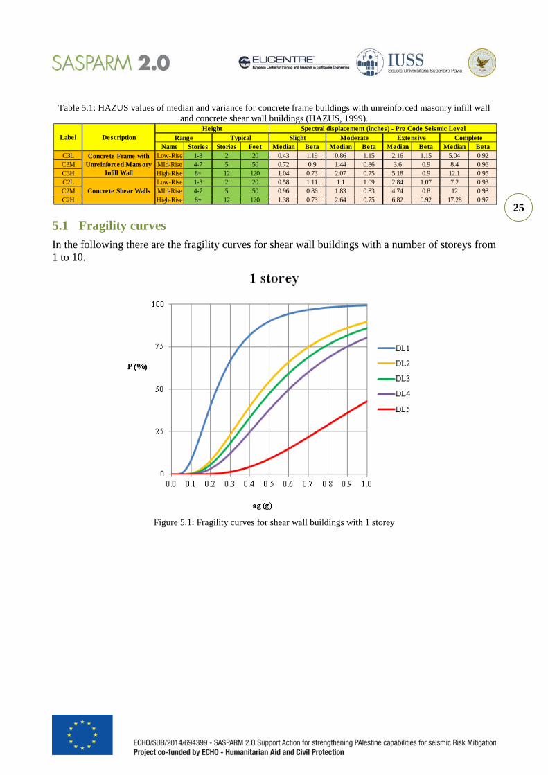
5 Fragility curves for concrete shear wall buildings ..................................................................... 24
5.1 Fragility curves .................................................................................................................... 25
6 References .................................................................................................................................. 30

iii
INDEX OF FIGURES
Figure 3.1: Capacity curve for elastic-perfectly-plastic structural behavior ...................................... 10
Figure 3.2: Illustration of the multi-degree-of-freedom (MDOF) system and corresponding single-degree-of-freedom (SDOF) system .................................................................................................... 10
Figure 3.3: Fragility curves for masonry buildings with 1 storey ...................................................... 15
Figure 3.4: Fragility curves for masonry buildings with 2 storeys .................................................... 15
Figure 3.5: Fragility curves for masonry buildings with 3 storeys .................................................... 15
Figure 3.6: Fragility curves for masonry buildings with 4 storeys .................................................... 16
Figure 4.1: Plan of the RC concrete frame building hired as a prototype for the analysis of vulnerability ....................................................................................................................................... 17
Figure 4.2: collapse mechanism: a) weak storey and b) global ......................................................... 17
Figure 4.3: a) One way ribbed slab system and b) Two way ribbed slab system .............................. 18
Figure 4.4: Fragility curves for RC frame buildings with 1 storey .................................................... 19
Figure 4.5: Fragility curves for RC frame buildings with 2 storeys .................................................. 20
Figure 4.6: Fragility curves for RC frame buildings with 3 storeys .................................................. 20
Figure 4.7: Fragility curves for RC frame buildings with 4 storeys .................................................. 21
Figure 4.8: Fragility curves for RC frame buildings with 5 storeys .................................................. 21
Figure 4.9: Fragility curves for RC frame buildings with 6 storeys .................................................. 22
Figure 4.10: Fragility curves for RC frame buildings with 7 storeys ................................................ 22
Figure 4.11: Fragility curves for RC frame buildings with 8 storeys ................................................ 23
Figure 4.12: Fragility curves for RC frame buildings with 9 storeys ................................................ 23
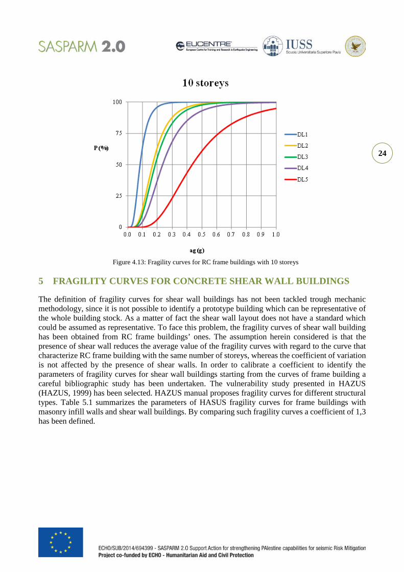
Figure 4.13: Fragility curves for RC frame buildings with 10 storeys .............................................. 24
Figure 5.1: Fragility curves for shear wall buildings with 1 storey ................................................... 25
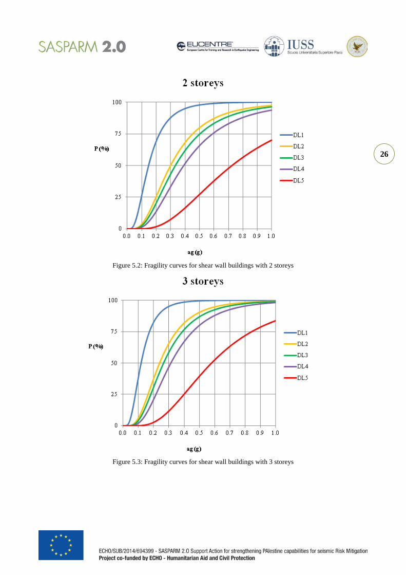
Figure 5.2: Fragility curves for shear wall buildings with 2 storeys .................................................. 26
Figure 5.3: Fragility curves for shear wall buildings with 3 storeys .................................................. 26
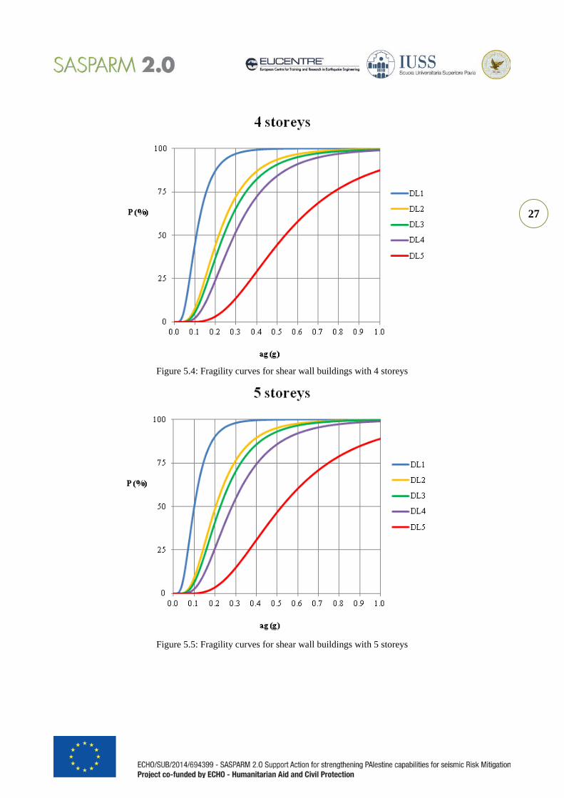
Figure 5.4: Fragility curves for shear wall buildings with 4 storeys .................................................. 27
Figure 5.5: Fragility curves for shear wall buildings with 5 storeys .................................................. 27
Figure 5.6: Fragility curves for shear wall buildings with 6 storeys .................................................. 28
Figure 5.7: Fragility curves for shear wall buildings with 7 storeys .................................................. 28
Figure 5.8: Fragility curves for shear wall buildings with 8 storeys .................................................. 29
Figure 5.9: Fragility curves for shear wall buildings with 9 storeys .................................................. 29
Figure 5.10: Fragility curves for shear wall buildings with 10 storeys .............................................. 30

iv
v
INDEX OF TABLES
Table 3.1: k1 and k2 coefficients as a function of number of floors (Restrepo-Velez 2003). ........... 11
Table 3.2: Correction factors for masonry buildings with high vulnerability. .................................. 14
Table 5.1: HAZUS values of median and variance for concrete frame buildings with unreinforced masonry infill wall and concrete shear wall buildings (HAZUS, 1999). ........................................... 25

7
1 INTRODUCTION
The WebGIS platform developed for this project allows to identify on the Nablus map the position of the buildings for which were compiled the collection forms by practitioners and citizens. These forms correspond to deliverable D.B.2. Using the information collected with the forms it is possible to assign to each building one of the structural typologies that classify the as built in Nablus, previously identified and described in deliverable D.B.1 such as:
• RC frame buildings; • Shear wall buildings; • Masonry Buildings; • RC frame buildings with soft storey.
The assigned typology, combined with the number of storeys of the building, allows to connect each building with a set of five fragility curves corresponding to damage levels ranging from D1 to D5 (from light damage to collapse) of the EMS98 scale (European Macroseismic Scale, Grünthal 1998). The assigned fragility curves are also displayed on the WebGIS platform and they are used for the seismic risk calculation together with the hazard curve.
The fragility curves have been developed starting from the SP-BELA (Simplified Pushover-Based Earthquake Loss Assessment) methodology, adapted on the reality of the as built in Nablus. The SP-BELA methodology (Borzi et al. 2008a, 2008b and 2008c) is a mechanic based method for the evaluation of the building capacity through the calculation of push-over curves conducted on populations of buildings statistically generated in order to be representative of the seismic behaviour of each structural type. The capability of SP-BELA method to represent the seismic performance of buildings in large scale assessment has been tested comparing the results of simulated damage scenario with damage observed during the post-event surveys in Italy from the earthquake of Friuli 1976 to the earthquake of Emilia 2012.
In order to define vulnerability curves it is necessary to identify a prototype building which is going to be representative of the building stock for each structural type. The properties of the prototype building are described through random variables in order to represent the uncertainties on the building response. For the random variables involving in the definition of the capacity curves, it has been necessary to specify the parameters (i.e. average and standard deviation if the distribution is normal) that describe their probabilistic distribution. In the next paragraphs the prototype buildings and the random variable adopted for their description are documented.
The limits of SP-BELA methodology are that using push-over curves to describe the building capacity, torsional modes cannot be taken into account. Such modes can play a role of RC buildings that very often have irregular layout in plan and elevation. To overcome this limit many analyses will be carried out to calculate a multiplication factor that takes into account the presence of torsional effects. This subject is described in deliverable D.F.2.
Furthermore, a global collapse mechanism is considered. Hence, for masonry buildings it is not possible to account for local mechanisms such as out of plane failure of masonry panels which characterize the high vulnerable buildings. To overcome this limitation the fragility curves have been calculated for global failure mechanism. The obtained curves are then corrected trough coefficients
8
that have been calibrated on the bases of observed damage on masonry buildings classified as high and low vulnerability during Italian earthquakes.
The fragility curve sets that have been calculated in this deliverable are:
1) Masonry buildings (with the number of storeys from 1 to 4 since a higher number of floors cannot be built with masonry);
2) R.C. frames with regular and irregular distribution of stiffness along the height. The number of storeys ranges from 1 to 10; if N storeys > 10 assumes 10 storeys since above a certain building height the vulnerability is not anymore a function of the number of storeys;
3) Shear wall buildings. The number of storeys ranges from 1 to 10; if N storeys > 10 assumes 10 storeys since above a certain building height the vulnerability is not anymore a function of the number of storey.
2 METHODOLOGY TO DEFINE THE FRAGILITY CURVES
The SP-BELA method, adopted to define the fragility curves, combines the definition of a pushover curve using a simplified mechanics based procedure to calculate the base shear capacity of the building stock, with a displacement-based framework, such that the vulnerability of building classes at different limit states can be obtained. The steps that lead to the fragility curve definition are:
1. Definition of a building sample of 1000 buildings through Monte Carlo generation: the structural type is identified by a building which does not have deterministic properties, but is described through random variables. The following five possible probability distribution have been taken into account: (i) normal distribution, (ii) log-normal distribution, (iii) constant distribution, (iv) random selection between a set of values and (v) constant value. The sample size of 1000 is considered to be statistically representative since its increase does not affect the results. The parameters which vary and generate the representative sample of a given class of buildings concern the geometry of the buildings, the loads applied to the buildings, the material characteristics and the deformation capacity.
2. Definition of building capacity through a pushover curve for each component of the building sample. On the pushover curve, the displacement values which define the achievement of selected limit conditions (e.i. light damage, significant damage and collapse) are identified. From the pushover curve it is possible to define the properties of an equivalent single degree of freedom system, which is equivalent to the original system in terms of period of vibration, displacement capacity and dissipation capacity. Latter is taken into account by means of an equivalent damping factor which can be defend as a function of ductility.
3. Definition of the displacement demand: a displacement spectral shape is anchored to each value of PGA for which the point of the fragility curve is calculated. The spectral shape was defined using the acceleration spectrum proposed by Eurocode 8 multiplied by (T/2π)2 to give the corresponding displacement spectrum for 5% damping. In the probabilistic procedure used to calculate the fragility curves, the uncertainty in the definition of the demand is accounted for by assuming the corner periods of the spectrum and the spectral amplification coefficient as a random variable;
9
4. Comparison between demand and capacity to define the proportion of buildings of the sample that survive the considered limit conditions. For example, if for 800 buildings of 1000 the demand for a predetermined acceleration value is greater than the capacity for the limit state of significant damage means that the fragility curve will be 80% for that acceleration value and that limit state. By varying the acceleration, it is then possible to build all the points of fragility curve for each limit state and then find the parameters (i.e. average and standard deviation) of the lognormal cumulative distribution that interpolates the calculated points.
SP-BELA is an analytical methodology that takes into account the limit states numerically identified. The steps described above allow to define fragility curves for the 3 mentioned limit states: light damage, significant damage and collapse. Recently it was decided to add an additional step which involves the shift from curves for three limit states to those for five damage levels (DL1, …, DL5) in reference to the five damage levels of EMS98 scale (Grünthal 1998). The relationship between damage levels and limit states has been defined on the basis of observed damage data in recent Italian earthquakes from Friuli 1976 to Emilia 2002.
In the following paragraphs, it is described more in detail each assumption that has been done for the calculation of the fragility curves.
3 FRAGILITY CURVES FOR MASONRY BUILDINGS
Masonry buildings were the most common in Nablus up to 1970. Masonry buildings comprise masonry walls that support reinforced concrete slabs. To characterize the behavior of masonry buildings, the failure mechanisms that can be activated when the building is subjected to an earthquake are classified in the (i) in plan collapse mechanisms and (ii) out of plan collapse mechanisms. In order to have a global collapse mechanism of the building, which involves the entire structure, it is necessary that the “in plan collapse mechanisms” are activated before the “out of plan collapse mechanisms”. The main cause of the “out of plan collapse mechanisms” activation is the absence of the edge beams and ties and the presence of design or construction errors. Lacking complete information concerning the presence or absence of the edge beams and ties and construction details in the masonry buildings of Nablus, in the numeric modeling for assessing the fragility curves were considered only the “in plan collapse mechanisms”. In this way fragility curves for good quality masonry would be obtained. Then to generate curves for poor quality masonry, more realistic for the Nablus building stock, correction factors calibrated on observed damage data after Italian earthquakes from 1976 (Friuli) to 2012 (Emilia) were applied (§3.4). The limit of adopting Italian observation data cannot be overcome since data for Palestine are not available.
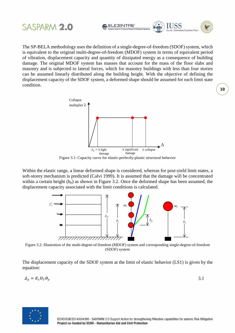
As mentioned in the previous paragraph, the fragility curves are obtained using the SP-BELA methodology. In this method the structural capacity is represented through a pushover curve, which represents the base-shear force of the structure under a lateral distribution of forces versus the displacement at a control point. During the pushover analysis, the forces increase until the structure reaches a collapse limit condition. For the masonry buildings the pushover curve is idealized through a bilinear curve, and an elastic perfectly plastic behavior is assumed. As a consequence, to define the pushover curve, only the collapse multiplier and the displacement capacities need to be calculated (Figure 3.1). On the pushover curve, the displacement capacity can be related to damage conditions that are identifiable with the limit states mentioned in the Chapter 2.
10
The SP-BELA methodology uses the definition of a single-degree-of-freedom (SDOF) system, which is equivalent to the original multi-degree-of-freedom (MDOF) system in terms of equivalent period of vibration, displacement capacity and quantity of dissipated energy as a consequence of building damage. The original MDOF system has masses that account for the mass of the floor slabs and masonry and is subjected to lateral forces, which for masonry buildings with less than four stories can be assumed linearly distributed along the building height. With the objective of defining the displacement capacity of the SDOF system, a deformed shape should be assumed for each limit state condition.
Figure 3.1: Capacity curve for elastic-perfectly-plastic structural behavior
Within the elastic range, a linear deformed shape is considered, whereas for post-yield limit states, a soft-storey mechanism is predicted (Calvi 1999). It is assumed that the damage will be concentrated within a certain height (hp) as shown in Figure 3.2. Once the deformed shape has been assumed, the displacement capacity associated with the limit conditions is calculated.
Figure 3.2: Illustration of the multi-degree-of-freedom (MDOF) system and corresponding single-degree-of-freedom
(SDOF) system
The displacement capacity of the SDOF system at the limit of elastic behavior (LS1) is given by the equation:
𝛥𝛥𝑦𝑦 = 𝐾𝐾1𝐻𝐻𝑇𝑇𝛩𝛩𝑦𝑦 3.1
∆y = ∆ light damage
∆ significant damage
∆ collapse ∆
Collapse multiplier λ
Fi
hThi
mi
hp
me
he
11
where K1 is the coefficient that is multiplied by HT, the total building height, to obtain the equivalent height of the SDOF system and θy is the drift at the limit of elastic behavior (Restrepo-Velez and Magenes 2004). If the building has a regular distribution of masses along the height, K1 is approximately 0.67. As a consequence of the assumption of a soft-story mechanism, the plastic deformations are concentrated within the height hp, which is considered herein to correspond to the interstory height. For buildings with a large number of openings, the soft-storey mechanism should be developed over a height that is greater than the opening height and less than the interstorey height. In this case, the use of the interstorey height would not be conservative because it would increase the building displacement capacity. This assumption is, however, acceptable because it compensates for the conservative assumptions that are typical within a mechanics-based vulnerability method where many contributions to the structural building resistance (e.g., contribution of partition walls) are neglected. Therefore, the displacement capacity for the limit states corresponding to a structure entering the non-linear range is:
𝛥𝛥𝐿𝐿𝐿𝐿𝐿𝐿 = 𝐾𝐾1𝐻𝐻𝑇𝑇𝛩𝛩𝑦𝑦 + 𝐾𝐾2�𝛩𝛩𝐿𝐿𝐿𝐿𝐿𝐿 − 𝛩𝛩𝑦𝑦�ℎ𝑝𝑝 3.2
where θLSi is the drift limit state capacity. For the evaluation of displacement capacity in the equations noted previously, the coefficients K1 and K2 need to be defined. For masses uniformly distributed along the building height and for walls with a mass equal to 30% of the floor mass, Restrepo-Velez (2003) has calculated K1 and K2 as summarized in Table 3.1.
Table 3.1: k1 and k2 coefficients as a function of number of floors (Restrepo-Velez 2003). Number of storeys K1 K2
1 0.790 0.967 2 0.718 0.950 3 0.698 0.918 4 0.689 0.916
These values are valid for the cases where collapse mechanisms are activated within the first two-thirds of the building height. Once the displacement capacity has been defined, to fully describe the pushover curve the collapse multipliers have to be calculated. As suggested by Restrepo-Velez and Magenes (2004), the formula given by Benedetti and Petrini (1984) can be used for the collapse multiplier li at the interstory i:
21
1
15,111
/
ABiki
n
ikk
kii
n
jjj
n
ikii
T
i )γ(Aτ
WτA
Wh
WhW
λ
++=
∑
∑
∑=
=
=
3.3
12
where: WT is the total weight of the building, Wi is the weight of the floor i, τki is the shear resistance of the masonry at floor i, Ai is the total area of resisting walls at level i in the direction of application of loads, γAB is the ratio between Ai and Bi with Bi being the maximum area between the area of wall in the loaded direction and the orthogonal direction, and n is the number of storeys. The building collapse multiplier will be the smallest amongst all of the calculated λi:
𝜆𝜆 = min{𝜆𝜆𝐿𝐿} 3.4
The formula of λi given by Benedetti and Petrini (1984) neglects 3D effects such as torsion due to an eccentricity between the center of stiffness and the center of mass of the building. Restrepo-Velez and Magenes (2004) have therefore suggested the introduction of a correction coefficient expressed by:
𝜆𝜆 = 𝛷𝛷𝑐𝑐−1min{𝜆𝜆𝐿𝐿} 3.5
The correction coefficient Φc has been defined through comparison with results of finite element analyses on three-dimensional buildings with the code SAM (Simplified Analysis of Masonry) that has been developed and verified by Magenes and Della Fontana (1998) and Magenes et al. (2000), among others. Through a regression analysis on the obtained results, Restrepo-Velez and Magenes (2004) have obtained the following formulation of Φc:
𝛷𝛷𝑐𝑐 = 5.5𝜏𝜏𝑘𝑘𝐿𝐿𝐿𝐿𝑊𝑊𝐿𝐿𝑇𝑇
+ 0.5 3.6
where LT is the total length of the walls in the direction of loads, and LW is the total length of the walls without openings in the loaded direction.
The next paragraph documents the variables adopted for the sample Monte Carlo generation in terms of geometry of the building (§3.1), applied loads (§3.2) and material characteristics and displacement capacity (§3.3). In the §3.4 the correction factors used to obtain the fragility curve for masonry buildings with high vulnerability starting from the curves for masonry buildings at low vulnerability are reported. Finally, in §3.5 the obtained fragility curves are shown.
3.1 Geometry of the building The first two variables are the resistant area of the walls in the seismic action direction (%) and the resistant area of the walls in the direction orthogonal to the seismic action (%). In the masonry buildings in Nablus typically the cross sectional area of walls is about 10 % from the floor area, so these variables are assumed with an average value of 10%, a standard deviation of 5% and a normal distribution.
Another variable is the percentage of length resistant walls with respect to the length of the external walls: it is assigned an average value of 66%, a standard deviation of 10% and a normal distribution. These values come from an elaboration of the data collected, at regional level, through the 2nd Level
13
Forms of GNDT in Italy (“Gruppo Nazionale per la Difesa dai Terremoti”) since specific data for the as built in Nablus are not available.
The last variable about the geometry is the interstory height: it is assigned an average value of 3.4 m, a standard deviation of 1.1 m and a normal distribution. Also these values come from the 2nd Level Forms of GNDT in Italy.
3.2 Loads The first two variables about the loads are the structural and non structural weight. From the Deliverable D.B.1 is known that the weight of the slab and the superimposed dead load is between 5 to 10 kN/m2. Therefore, to the structural weight it is assigned an average value of 4 kN/m2, a standard deviation of 2 kN/m2 and a normal distribution and to the non structural weight it is assigned an average value of 3 kN/m2, a standard deviation of 1 kN/m2 and a normal distribution.
An important load for the buildings in Nablus is the weight of water tanks located on the top of the structure. In case the building with a roof slab, the load shall be added on the roof slab with a value of 1 kN/m2 per story number. Otherwise, if the building does not have a roof slab, the load shall be added to the last floor of the building and has a value of 0.5 kN/m2 per story number. In the vulnerability curves evaluation this variable is assigned as a random selection between 1 and 0.5 kN/m2 multiplied by the number stories. To the variable related with the specific weight of the masonry is assigned a constant value of 25 kN/m3 as suggested in the Deliverable D.B.1.
Last variable that describes the load is the live load and is represented by a constant value of 3 kN/m2. No variability is given to the life load, since only a percentage of it is considered to evaluate the seismic building performance, hence the lead does not have a predominate influence.
3.3 Material Characteristics and deformation capacity In order to define the in plane capacity of the walls and their displacement capacity the tangential stress and the interstory rotation capacity have to be defined. From the Deliverable D.B.1 is known that the shear resistance of the block walls is between 40 kN/m2 to 100 kN/m2, then the variable related to the tangential stress is assumed to be a constant distribution between these two values. At last for the interstory rotations are assumed the values from literature (Magenes et al. (1997) for light damage and severe damage limit state and Magenes (1992) for the ultimate limit state. In particular, for the light damage limit state a normal distribution with an average value of 0.13% and a standard deviation of 0.046% is assumed; for the severe damage limit state a normal distribution with an average value of 0.34% and a standard deviation of 0.102% is assumed; for the ultimate limit state a normal distribution with an average value of 0.72% and a standard deviation of 0.252% is assumed.
3.4 Correction factors For masonry buildings, the SP-BELA method is unable to describe the behavior of the buildings in high vulnerability class, like those in Nablus, due to the lack of the necessary information. Therefore, to evaluate the fragility of masonry buildings a hybrid procedure that combines the mechanic methodology SP-BELA, which produces fragility curves for good quality masonry, with the results of observations on earthquakes in the past was adopted. As mentioned above, to account for the
14
observations, the damage data after Italian earthquakes from 1976 (Friuli) to 2012 (Emilia) were adopted.
Comparing the damage scenarios calculated with SP-BELA method versus the observed damage data has been possible to calibrate the correction factors that relate the fragility curves for masonry buildings with high vulnerability with those with low vulnerability. The correction factors obtained are reported in Table 3.2. The fragility curves for high vulnerable buildings can be obtained by dividing the average through the factors in Table 3.2 and maintaining fixed the coefficient of variation CV (CV=standard deviation/abs(average)) of the curves for low vulnerable buildings. The correction factors vary as a function of the damage level: in Table 3.2 only the factors for damage level DL3 and DL4 are shown, because the curves for the other damage levels are derived from the latter, as explained in Chapter 2.
Table 3.2: Correction factors for masonry buildings with high vulnerability. Damage level Correction factors DL3 2.8 DL4 2.3
3.5 Fragility curves
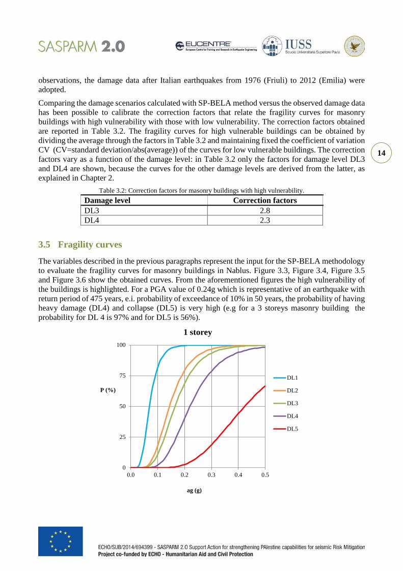
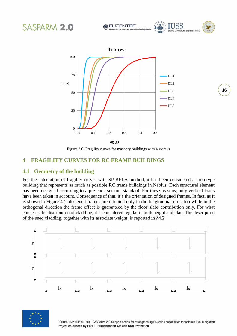
The variables described in the previous paragraphs represent the input for the SP-BELA methodology to evaluate the fragility curves for masonry buildings in Nablus. Figure 3.3, Figure 3.4, Figure 3.5 and Figure 3.6 show the obtained curves. From the aforementioned figures the high vulnerability of the buildings is highlighted. For a PGA value of 0.24g which is representative of an earthquake with return period of 475 years, e.i. probability of exceedance of 10% in 50 years, the probability of having heavy damage (DL4) and collapse (DL5) is very high (e.g for a 3 storeys masonry building the probability for DL 4 is 97% and for DL5 is 56%).
0
25
50
75
100
0.0 0.1 0.2 0.3 0.4 0.5
P (%)
ag (g)
1 storey
DL1
DL2
DL3
DL4
DL5

15
Figure 3.3: Fragility curves for masonry buildings with 1 storey
Figure 3.4: Fragility curves for masonry buildings with 2 storeys
Figure 3.5: Fragility curves for masonry buildings with 3 storeys
0
25
50
75
100
0.0 0.1 0.2 0.3 0.4 0.5
P (%)
ag (g)
2 storeys
DL1
DL2
DL3
DL4
DL5
0
25
50
75
100
0.0 0.1 0.2 0.3 0.4 0.5
P (%)
ag (g)
3 storeys
DL1
DL2
DL3
DL4
DL5
16
Figure 3.6: Fragility curves for masonry buildings with 4 storeys
4 FRAGILITY CURVES FOR RC FRAME BUILDINGS
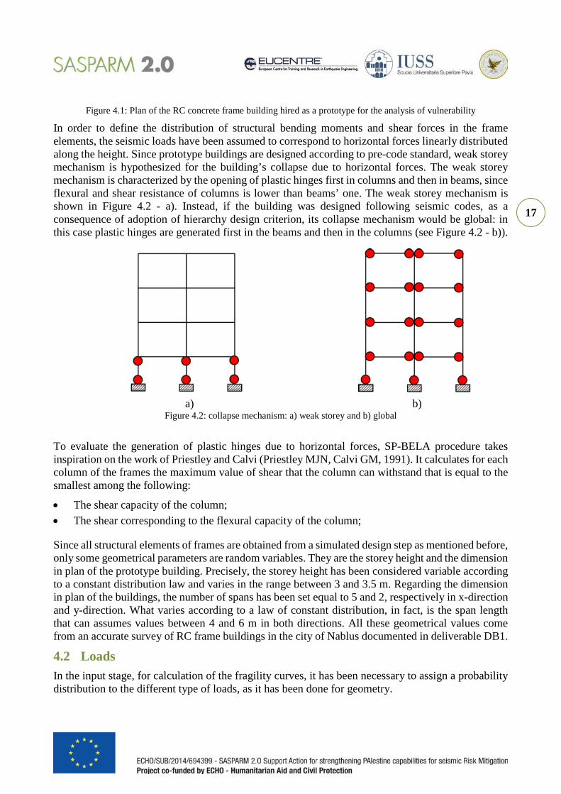
4.1 Geometry of the building For the calculation of fragility curves with SP-BELA method, it has been considered a prototype building that represents as much as possible RC frame buildings in Nablus. Each structural element has been designed according to a pre-code seismic standard. For these reasons, only vertical loads have been taken in account. Consequence of that, it’s the orientation of designed frames. In fact, as it is shown in Figure 4.1, designed frames are oriented only in the longitudinal direction while in the orthogonal direction the frame effect is guaranteed by the floor slabs contribution only. For what concerns the distribution of cladding, it is considered regular in both height and plan. The description of the used cladding, together with its associate weight, is reported in §4.2.
0
25
50
75
100
0.0 0.1 0.2 0.3 0.4 0.5
P (%)
ag (g)
4 storeys
DL1
DL2
DL3
DL4
DL5
ly
ly
lx lx lx lx lx
17
Figure 4.1: Plan of the RC concrete frame building hired as a prototype for the analysis of vulnerability
In order to define the distribution of structural bending moments and shear forces in the frame elements, the seismic loads have been assumed to correspond to horizontal forces linearly distributed along the height. Since prototype buildings are designed according to pre-code standard, weak storey mechanism is hypothesized for the building’s collapse due to horizontal forces. The weak storey mechanism is characterized by the opening of plastic hinges first in columns and then in beams, since flexural and shear resistance of columns is lower than beams’ one. The weak storey mechanism is shown in Figure 4.2 - a). Instead, if the building was designed following seismic codes, as a consequence of adoption of hierarchy design criterion, its collapse mechanism would be global: in this case plastic hinges are generated first in the beams and then in the columns (see Figure 4.2 - b)).
a) b)
Figure 4.2: collapse mechanism: a) weak storey and b) global
To evaluate the generation of plastic hinges due to horizontal forces, SP-BELA procedure takes inspiration on the work of Priestley and Calvi (Priestley MJN, Calvi GM, 1991). It calculates for each column of the frames the maximum value of shear that the column can withstand that is equal to the smallest among the following:
• The shear capacity of the column; • The shear corresponding to the flexural capacity of the column;
Since all structural elements of frames are obtained from a simulated design step as mentioned before, only some geometrical parameters are random variables. They are the storey height and the dimension in plan of the prototype building. Precisely, the storey height has been considered variable according to a constant distribution law and varies in the range between 3 and 3.5 m. Regarding the dimension in plan of the buildings, the number of spans has been set equal to 5 and 2, respectively in x-direction and y-direction. What varies according to a law of constant distribution, in fact, is the span length that can assumes values between 4 and 6 m in both directions. All these geometrical values come from an accurate survey of RC frame buildings in the city of Nablus documented in deliverable DB1.
4.2 Loads In the input stage, for calculation of the fragility curves, it has been necessary to assign a probability distribution to the different type of loads, as it has been done for geometry.
18
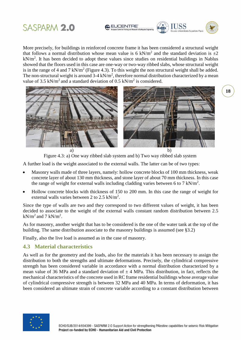
More precisely, for buildings in reinforced concrete frame it has been considered a structural weight that follows a normal distribution whose mean value is 6 kN/m2 and the standard deviation is ±2 kN/m2. It has been decided to adopt these values since studies on residential buildings in Nablus showed that the floors used in this case are one-way or two-way ribbed slabs, whose structural weight is in the range of 4 and 7 kN/m2 (Figure 4.3). To this weight the non structural weight shall be added. The non-structural weight is around 3-4 kN/m2, therefore normal distribution characterized by a mean value of 3.5 kN/m2 and a standard deviation of 0.5 kN/m2 is considered.
a) b)
Figure 4.3: a) One way ribbed slab system and b) Two way ribbed slab system
A further load is the weight associated to the external walls. The latter can be of two types:
• Masonry walls made of three layers, namely: hollow concrete blocks of 100 mm thickness, weak concrete layer of about 130 mm thickness, and stone layer of about 70 mm thickness. In this case the range of weight for external walls including cladding varies between 6 to 7 kN/m2.
• Hollow concrete blocks with thickness of 150 to 200 mm. In this case the range of weight for external walls varies between 2 to 2.5 kN/m2.
Since the type of walls are two and they correspond to two different values of weight, it has been decided to associate to the weight of the external walls constant random distribution between 2.5 kN/m2 and 7 kN/m2.
As for masonry, another weight that has to be considered is the one of the water tank at the top of the building. The same distribution associate to the masonry buildings is assumed (see §3.2)
Finally, also the live load is assumed as in the case of masonry.
4.3 Material characteristics As well as for the geometry and the loads, also for the materials it has been necessary to assign the distribution to both the strengths and ultimate deformations. Precisely, the cylindrical compressive strength has been considered variable in accordance with a normal distribution characterized by a mean value of 36 MPa and a standard deviation of ± 4 MPa. This distribution, in fact, reflects the mechanical characteristics of the concrete used in RC frame residential buildings whose average value of cylindrical compressive strength is between 32 MPa and 40 MPa. In terms of deformation, it has been considered an ultimate strain of concrete variable according to a constant distribution between
19
0,3% and 0,8%. As regards the steel, instead, it has been considered a tensile strength equal to 420 MPa and a ultimate deformation variable according to a constant distribution between 1% to 3%.
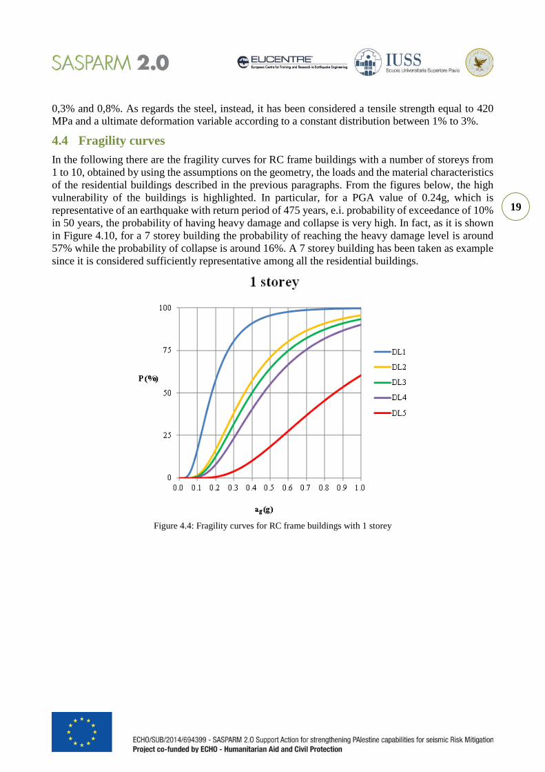
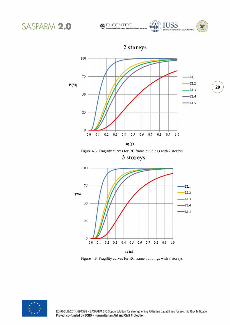
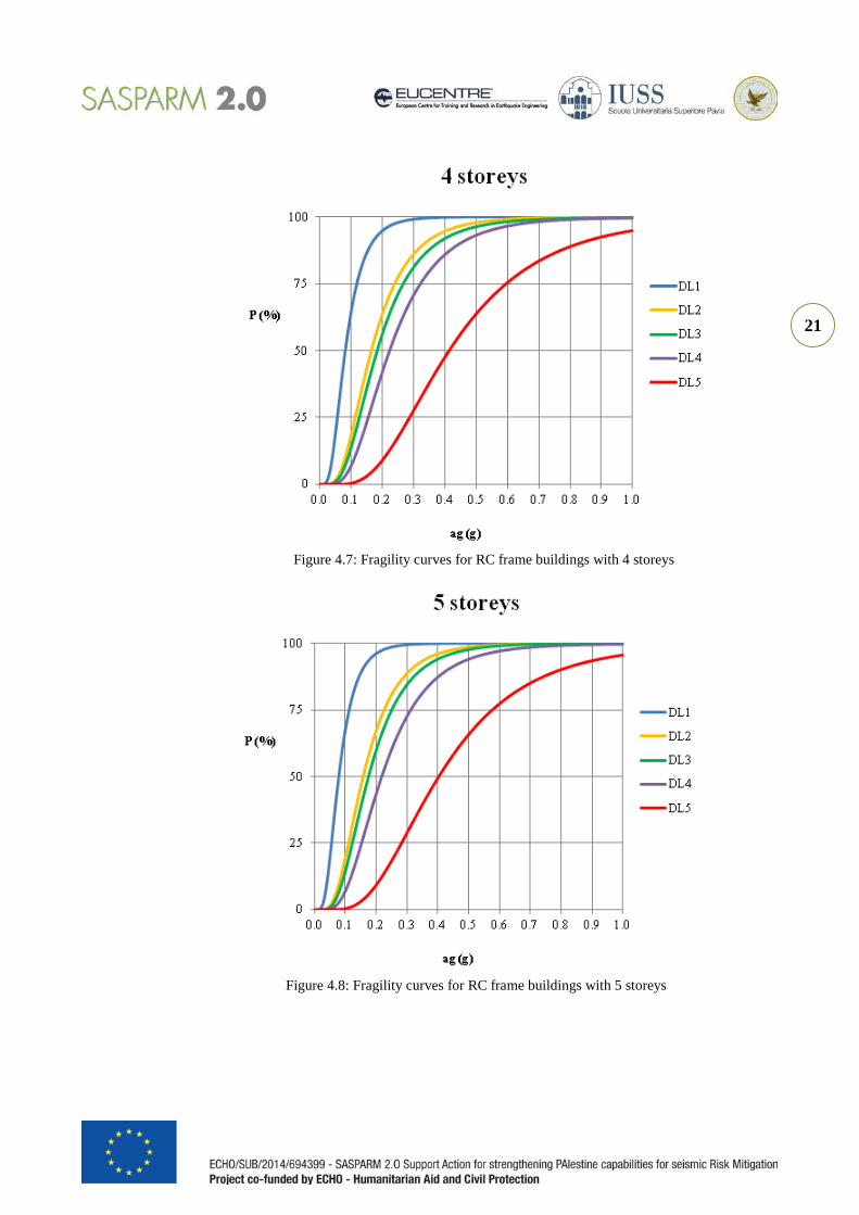
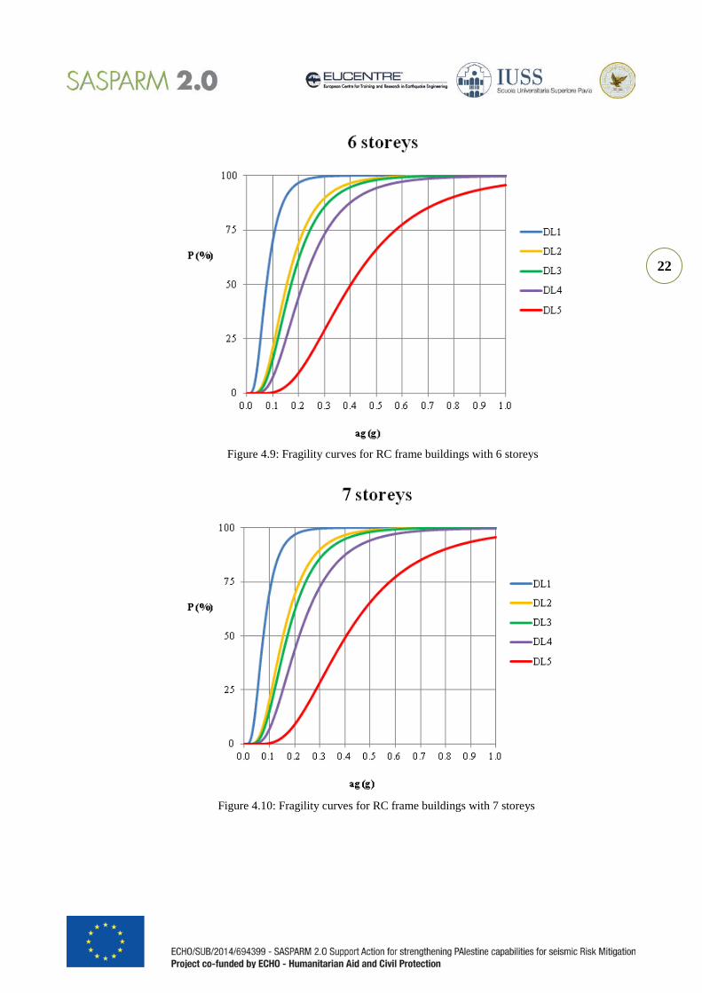
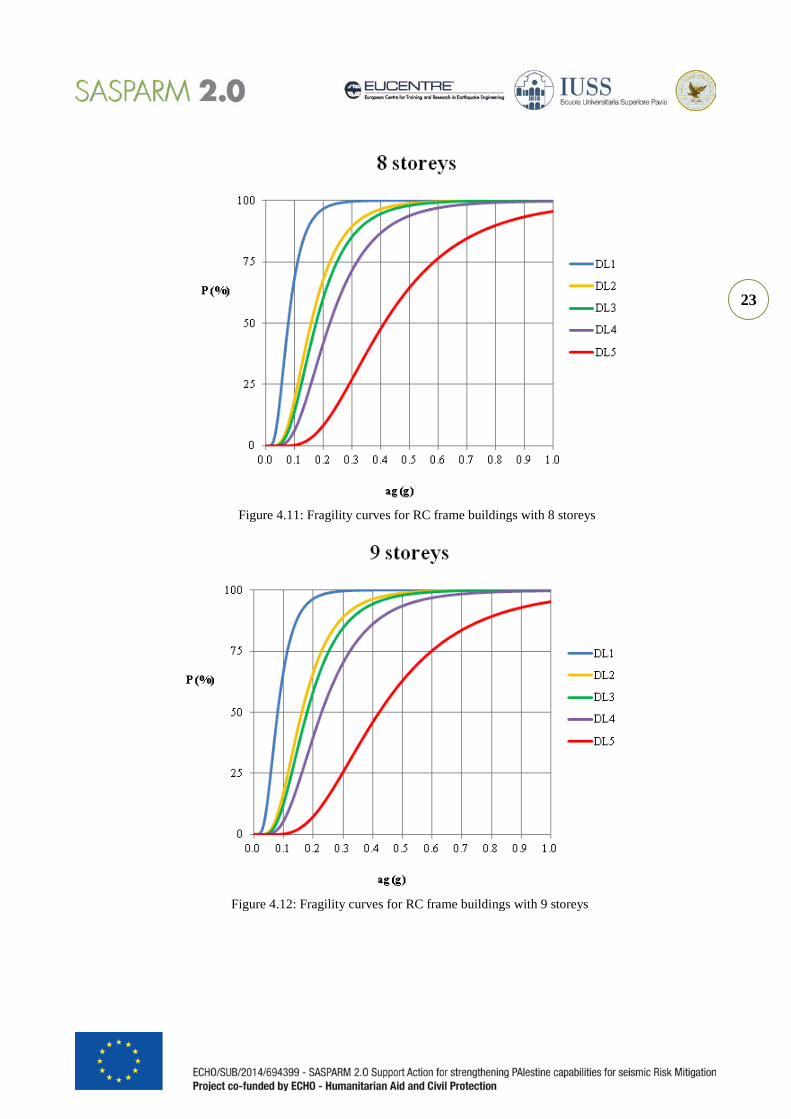
4.4 Fragility curves In the following there are the fragility curves for RC frame buildings with a number of storeys from 1 to 10, obtained by using the assumptions on the geometry, the loads and the material characteristics of the residential buildings described in the previous paragraphs. From the figures below, the high vulnerability of the buildings is highlighted. In particular, for a PGA value of 0.24g, which is representative of an earthquake with return period of 475 years, e.i. probability of exceedance of 10% in 50 years, the probability of having heavy damage and collapse is very high. In fact, as it is shown in Figure 4.10, for a 7 storey building the probability of reaching the heavy damage level is around 57% while the probability of collapse is around 16%. A 7 storey building has been taken as example since it is considered sufficiently representative among all the residential buildings.
Figure 4.4: Fragility curves for RC frame buildings with 1 storey
20
Figure 4.5: Fragility curves for RC frame buildings with 2 storeys
Figure 4.6: Fragility curves for RC frame buildings with 3 storeys
21
Figure 4.7: Fragility curves for RC frame buildings with 4 storeys
Figure 4.8: Fragility curves for RC frame buildings with 5 storeys
22
Figure 4.9: Fragility curves for RC frame buildings with 6 storeys
Figure 4.10: Fragility curves for RC frame buildings with 7 storeys
23
Figure 4.11: Fragility curves for RC frame buildings with 8 storeys
Figure 4.12: Fragility curves for RC frame buildings with 9 storeys
24
Figure 4.13: Fragility curves for RC frame buildings with 10 storeys
5 FRAGILITY CURVES FOR CONCRETE SHEAR WALL BUILDINGS
The definition of fragility curves for shear wall buildings has not been tackled trough mechanic methodology, since it is not possible to identify a prototype building which can be representative of the whole building stock. As a matter of fact the shear wall layout does not have a standard which could be assumed as representative. To face this problem, the fragility curves of shear wall building has been obtained from RC frame buildings’ ones. The assumption herein considered is that the presence of shear wall reduces the average value of the fragility curves with regard to the curve that characterize RC frame building with the same number of storeys, whereas the coefficient of variation is not affected by the presence of shear walls. In order to calibrate a coefficient to identify the parameters of fragility curves for shear wall buildings starting from the curves of frame building a careful bibliographic study has been undertaken. The vulnerability study presented in HAZUS (HAZUS, 1999) has been selected. HAZUS manual proposes fragility curves for different structural types. Table 5.1 summarizes the parameters of HASUS fragility curves for frame buildings with masonry infill walls and shear wall buildings. By comparing such fragility curves a coefficient of 1,3 has been defined.
25
Table 5.1: HAZUS values of median and variance for concrete frame buildings with unreinforced masonry infill wall and concrete shear wall buildings (HAZUS, 1999).
5.1 Fragility curves In the following there are the fragility curves for shear wall buildings with a number of storeys from 1 to 10.
Figure 5.1: Fragility curves for shear wall buildings with 1 storey
Name Stories Stories Feet Median Beta Median Beta Median Beta Median BetaC3L Low-Rise 1-3 2 20 0.43 1.19 0.86 1.15 2.16 1.15 5.04 0.92C3M MId-Rise 4-7 5 50 0.72 0.9 1.44 0.86 3.6 0.9 8.4 0.96C3H High-Rise 8+ 12 120 1.04 0.73 2.07 0.75 5.18 0.9 12.1 0.95C2L Low-Rise 1-3 2 20 0.58 1.11 1.1 1.09 2.84 1.07 7.2 0.93C2M MId-Rise 4-7 5 50 0.96 0.86 1.83 0.83 4.74 0.8 12 0.98C2H High-Rise 8+ 12 120 1.38 0.73 2.64 0.75 6.82 0.92 17.28 0.97
Label DescriptionHeight Spectral displacement (inches) - Pre Code Seismic Level
Range Typical Slight Moderate Extensive Complete
Concrete Frame with Unreinforced Mansory
Infill Wall
Concrete Shear Walls
26
Figure 5.2: Fragility curves for shear wall buildings with 2 storeys
Figure 5.3: Fragility curves for shear wall buildings with 3 storeys
27
Figure 5.4: Fragility curves for shear wall buildings with 4 storeys
Figure 5.5: Fragility curves for shear wall buildings with 5 storeys

28
Figure 5.6: Fragility curves for shear wall buildings with 6 storeys
Figure 5.7: Fragility curves for shear wall buildings with 7 storeys

29
Figure 5.8: Fragility curves for shear wall buildings with 8 storeys
Figure 5.9: Fragility curves for shear wall buildings with 9 storeys
30
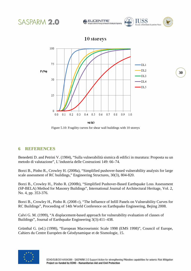
Figure 5.10: Fragility curves for shear wall buildings with 10 storeys
6 REFERENCES
Benedetti D. and Petrini V. (1984), “Sulla vulnerabilità sismica di edifici in muratura: Proposta su un metodo di valutazione”, L’industria delle Costruzioni 149: 66–74. Borzi B., Pinho R., Crowley H. (2008a), “Simplified pushover-based vulnerability analysis for large scale assessment of RC buildings,” Engineering Structures, 30(3), 804-820. Borzi B., Crowley H., Pinho R. (2008b), “Simplified Pushover-Based Earthquake Loss Assessment (SP-BELA) Method for Masonry Buildings”, International Journal of Architectural Heritage, Vol. 2, No. 4, pp. 353-376. Borzi B., Crowley H., Pinho R. (2008 c), “The Influence of Infill Panels on Vulnerability Curves for RC Buildings”, Proceeding of 14th World Conference on Earthquake Engineering, Bejing 2008. Calvi G. M. (1999), “A displacement-based approach for vulnerability evaluation of classes of Buildings”, Journal of Earthquake Engineering 3(3):411–438. Grünthal G. (ed.) (1998), “European Macroseismic Scale 1998 (EMS 1998)”, Council of Europe, Cahiers du Centre Européen de Géodynamique et de Sismologie, 15.
31
HAZUS (1999), “Earthquake Loss Estimation Methodology”, HAZUS ® 99, Service Release 2 (SR2) Technical Manual, Developed by: Federal Emergency Management Agency, Washington D.C: Through agreements with: national Institute of Building Science, Washington D.C. Magenes G. (1992), “Comportamento sismico di murature di mattoni: resistenza e meccanismi di rottura di maschi murari”, PhD Thesis, Department of Structural Mechanics, University of Pavia. Magenes G., Kingsley G.R., Calvi G.M. (1997), “Seismic testing of a full-scale, two-story masonry building: Test procedure and measure experimental response”, Gruppo Nazionale per la Difesa dai Terremoti. Magenes G. and Della Fontana A. (1998), “Simplified non-linear seismic analysis of masonry buildings”, Proceedings of the British Masonry Society 8:190–195. Magenes G., Bolognini D. and Baggio C. (2000), “Metodi semplificati per l’analisi sismica non lineare di edifici in muratura”, Rome, Italy: CNR-Gruppo Nazionale per la Difesa dai Terremoti. Priestley M.J.N., Calvi G.M. (1991), “Towards a capacity design assessment procedure for reinforced concrete frames”, Earthquake Spectra 1991;7(3): 413–37. Restrepo-Velez L.F. (2003), “A simplified mechanics-based procedure for the seismic risk assessment of unreinforced masonry buildings”, Individual Study. Pavia, Italy: ROSE School. Restrepo-Velez L.F. and Magenes G. (2004), “Simplified procedure for the seismic risk assessment of unreinforced masonry buildings”, Proceedings of the Thirteenth World Conference on Earthquake Engineering, Vancouver, Canada, paper no. 2561.