Supporting a Robust Decision Space

Gary L. Klein1, Mark Pfaff2, and Jill L. Drury3

The MITRE Corporation1, 3 and Indiana University – Indianapolis2 17515 Colshire Drive, McLean, VA 22102 USA

2 IT 469, 535 W. Michigan Street, Indianapolis, IN 46202 USA 3202 Burlington Road, Bedford, MA 01730 USA

Abstract A decision space is defined by the range of options at the decision maker’s disposal. For each option there is a distribution of possible consequences. Each distribution is a function of the uncertainty of elements in the decision situation (how big is the fire) and uncertainty regarding executing the course of actions defined in the decision option (what percent of fire trucks will get to the scene and when). To aid decision-makers, we can use computer models to visualize this decision space – explicitly representing the distribution of consequences for each decision option. Because decisions for dynamic domains like emergency response need to be made in seconds or minutes, the underlying (possibly complex) simulation models will need to frequently recalculate the myriad plausible consequences of each possible decision choice. This raises the question of the essential precision and fidelity of such simulations that are needed to support such decision spaces. If we can avoid needless fidelity that does not substantially change the decision space, then we can save development cost and computational time, which in turn will support more tactical decision-making. This work explored the trade space of necessary precision/fidelity of simulation models that feed data to decision-support tools. We performed sensitivity analyses to determine breakpoints where simulations become too imprecise to provide decision-quality data. The eventual goal of this work is to provide general principles or a methodology for determining the boundary conditions of needed precision/fidelity.

Introduction There is a large body of research literature surrounding situation awareness, defined by Endsley (1988) as the “the perception of the elements in the environment within a volume of time and space, the comprehension of their meaning and the projection of their status in the near future”. Using this definition, the information needed to attain situation awareness consists of facts about the environment, which Hall et al. (2007) call the situation space.

Copyright © 200 , Association for the Advancement of Artificial Intelligence (www.aaai.org). All rights reserved.

Yet, truly aiding decision makers requires providing them with more than situational facts. Decision makers must choose among the options for action that are at their disposal. This additional view of the environment is termed the decision space (Hall et al., 2007). Decision makers therefore must be able to compare these options in the decision space and choose among them, given an analysis of the facts of the situation, which maps from the facts to the consequences of each option. For each option there is a distribution of possible consequences. Each distribution is a function of the uncertainty of the elements in the decision situation (how big is the fire) and the uncertainty regarding executing the course of action defined in the decision option (what percent of fire trucks will get to the scene and when).

An optimal plan is one that will return the highest expected return on investment. However, under deep uncertainty (Lempert et. al. 2006), where situation and execution uncertainty are irreducible, optimal strategies lose their prescriptive value if they are sensitive to these uncertainties. That is, selecting an optimal strategy is problematic when there are multiple plausible futures.

Consider a very simple example. Suppose three is the optimal number of fire trucks to send to a medium-sized fire under calm wind conditions, but if conditions get windy, a higher number of trucks would be optimal. If your weather model predicts calm and windy conditions with equal probability, then what will be the optimal number of trucks? One could expend a lot of effort trying to improve the modeling of the weather in order to determine the answer. Furthermore, just how certain are you that the initial reported size of the fire is correct?

Alternatively, Chandresekaran (2005) and Chandresekaran & Goldman (2007) note that for course of action planning under deep uncertainty one can shift from seeking optimality to seeking robustness. In other words, one could look for the most robust line of approach that would likely be successful whether or not it will be windy.

Lempert, et al. (2006) describes a general simulation-based method for identifying robust strategies, a method they call robust decision making (RDM). Using our simple example, one would translate sending different numbers of fire trucks into the parameters of a

9

66

msmeurthvptuadin

thrtrohsuvbddeaeevcthsocvocthineo

ep

F

model. Then systematically model (e.g. weeach combinatiuncertainties trelatively well hat the model

vulnerabilities plausible circuurn, this can su

against these vdecision makern their decision

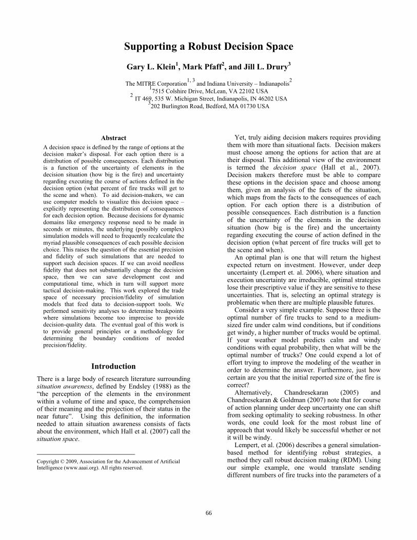
Figure 1 illuhis approach t

response situatrucks to send,

of the graph, whyperspace ofsummarized in used here mevisualization obe readily traindecision spacedecision visuaeach value of actual number estimated and executions of tvariables that course of actiohe wind in

systematically of the modelcombinations ovariable valuesof plausible fucan then be evhis case, the cnjury) is gener

evaluations foroption can be su

When the coeach course oprojection that

Figure 1: A decis

for each optimanipulate theather). The moion of numberto determine across the ranprojects. This of these optio

umstance eachuggest new opvulnerabilities.rs to characterin space of diffe

ustrates the reto a fire truck tion. Each optwhich is listed

was analyzed inf futures unFigure 1 as a

erely for illuption that typned to read. Oes will requialization meth

this endogenoof trucks that systematicall

the model. In would not be

on, but would lour simple

varied across l. The resultof different ens, which can buture situationsvaluated in terost of immediarated by that sir the hyperspacummarized graost of each siof action, weallows us to c

sion space visua

ion, one coule other uncertaodel would be r of trucks sen

which optionge of the plau

approach can ons, showing

h does well orptions to try to . Ultimately, ize the trade-o

ferent options.

sults of the apdecision in an

tion for a numd along the hon a simulation

nder a givena box plot. Theustration, as ical research Of course, more more dom

hods. Uncertaious variable, would arrive y varied acroaddition, othe

e under the clikely interact e example), these multiple

t was a hypndogenous ande considered as. Each of therms of how mate and future tuation. The re

ce of futures unaphically. ituation is mape get a two-compare robus

alization

ld explicitly ainties of the executed for

nt and set of on performs usible futures also identify under what

r poorly. In better hedge this enables

offs involved

pplication of n emergency mber of fire orizontal axis n model. The n option is e box plot is a common

subjects can ore complex main-specific inty around such as the in time, was oss multiple er exogenous control of a with it (like were also

e executions perspace of d exogenous a hyperspace se situations

much cost (in damage and

esult of these nder a given

pped against -dimensional stness in the

useFigsenmerelcasbettrureg

regsimrobmocanfouaconHosubsavwhmabe duof betcousou

detappsubhig

invverderneemefidowconpridecplaand

A dev(Jodevproevetessitu

ers’ decision sgure 1. In this nding 1 fire truedian cost (thlatively small ses and the ctween the “wh

uck seems to garding the uncThis decision

garding the reqmulations that bust decision odeling an exten be computatiund it is not unmodel, requirnsequences oowever, if we cbstantially chave model devehich in turn aking. Certainl

to cause a che to changes icosts. It cou

tween optionsuld also meanurce of each coIn this work, termine the leparent costs ubstantially fromgher-fidelity mThis work co

vestigation. Wry different mrive general pedless fidelityethodology so delity boundarywn models. Anntext of eminciples will becision-making ace on similar d control.

first test casveloped for thones et al., 20velopers: “Neogram designeents and occurst team decisiouations of eme

space, as illustrcase, across aluck seems to rhe line insiderange betwee

cost of the bhiskers”). In oth

be the most certainties inhen-space constrquired precision

actually are spaces. This

ensive set of pionally expensnusual to need ring days or of the optioncan avoid needange the deciselopment cost will support ly, one such shange in the rain the estimateuld also be a s’ median cosn a change inost point. sensitivity ana

evels of fidelitunder a lowerm the costs of

model. onstitutes the We are performmodels to deterinciples or gu

y. Furthermorthat others ca

y conditions and while we pe

mergency respe applicable tois of similar ctimescales, su

Backgrose of this re

he NeoCITIES 04). In the w

eoCITIES is aed to display irrences in a viron-making anergency crisis

rated by the bol of the plausib

result in not one the box), bn the cost of

best cases (thher words, Sen

robust decisierent in the situruction raisesn and fidelity oneeded to sup

s is importanpossible future ive. In our wormillions of ruweeks, to co

ns for somedless fidelity thsion space, theand computatimore tactical

substantial chanank order of ted median cost

change in thts or ranges.

n the situation

alyses were perty at which thr-fidelity modethe same optio

first phase oming similar ermine whetheuidelines for ere, we aim to an quickly deteand breakpointerformed the w

ponse, we beo other domaincomplexity anduch as military

undesearch was t

scaled-world words of the Nan interactive nformation pertual city spaced resource allmanagement”

ox plots in ble futures, nly a lower but also a f the worst he distance nding 1 fire ion option uation

questions of complex pport such nt because conditions

rk we have uns through mpute the decisions.

at does not en we can ional time, l decision-nge would the options ts or range

he distance Finally, it

ns that are

rformed to he options’ el differed ons using a

of a larger studies on er we can eliminating develop a

ermine the ts for their work in the elieve the ns in which d must take y command

the model simulation

NeoCITIES computer

ertaining to e, and then location in (McNeese

67

et al., 2005, p. 591). Small teams interact with NeoCITIES to assign police, fire/rescue, or hazardous materials assets in response to emerging and dynamic situations. If team members fail to allocate appropriate resources to an emergency event, the magnitude of the event grows over time until a failure occurs, such as the building burning to the ground or the event timing out.

The NeoCITIES model is designed to run in real time for human-in-the-loop (HIL) simulations. This provides a fast platform to rapidly test the core principles of this modeling research, whereas a high-fidelity version of a disease-spread model we are using in a parallel study can require days or weeks to run. In addition, this work will form the foundation for later HIL research to test the psychological implications of these model manipulations.

The heart of the NeoCITIES model is the magnitude equation, which dictates the growth of emergency events over time given an initial event magnitude score in the range of 1 – 5. It is the core equation in determining the distribution of costs for each option in the decision space. The calculation of this equation also drives the computational cost of each run of NeoCITIES, in terms of computer processing resources needed. Therefore it is the fidelity and precision of this equation that will be manipulated in this study.

The equation is time step-based and incremental: it depends upon the magnitude calculated for the previous time step t – 1 and the number of emergency resources (such as fire trucks) applied at that moment. This means that the magnitude of an event at a given time t cannot be obtained without calculating all of the magnitudes at all of the previous times, which is very computationally intensive. The full magnitude equation at time step t is:

��� � �� ���� � � ���� � � ��

where a, b, and c are weights and R is the number of resources applied. We represented the relationship between these factors in a number of computationally simpler ways as described in the methodology section.

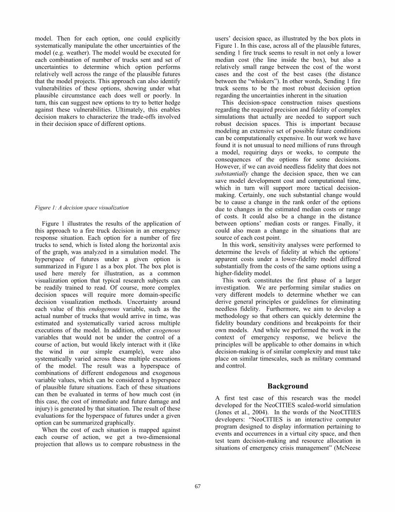
The magnitude equation determined whether assigning a given number of resources R at time step t is effective in resolving the emergency situation. Figure 2 shows a series of six curves that depict the effect over time of applying 0, 1, 2, 3, 4, or 5 resources

to a magnitude 3 event at time step t. Sending only 0 or 1 resource results in the event spiraling out of control within 40 time steps in the case of allocating 0 resources or sometime greater than 60 time steps in the case of allocating 1 resource. Sending 2 – 5 resources, results in resolving the emergency within 37 – 13 time steps, with the higher numbers of resources resolving the emergency more quickly, as might be expected.

To map this situational information into the decision space a way of costing the results of each option was needed. NeoCITIES’ original scoring equation assigned a combined cost to each resource allocation choice based on the number of expected deaths, injuries, and property damage as well as the cost of sending the designated number of resources. But this formulation did not incorporate the penalty that a decision maker might reasonably expect to pay if he or she assigned too many resources to an event and another event occurred before the first one could be resolved, with the result that the second event suffered more damage because insufficient resources were available nearby. Accordingly, we added to the cost of the current emergency any extra costs that would befall future emergencies due to over-allocating resources to the current emergency.

To determine the distribution of costs for each possible option for a given decision, we ran the model many times each under different conditions that are not under decision makers’ control. For example, imagine a fire in which a hot, dry wind fans the flames, versus a sudden downpour that dramatically diminishes the fire. Sending the same number of fire trucks in both situations will result in very different levels of damage; this uncertainty requires a range of costs be calculated for each option rather than a single point value.

MethodologyDevelopment of the models Two non-incremental equations were developed to model the incremental NeoCITIES escalation equation in a computationally simpler fashion. Being non-incremental, these equations can calculate the magnitude of an event for any time without calculating previous time steps, and therein reduce computational costs. However, the reduced fidelity of these non-incremental models, as compared to the “ground-truth” of the original NeoCITIES equation, provides one test of the fidelity boundary conditions – where simpler models may lead to recommending different options.

The first equation took a quadratic form: ��� � ��� � �� � ���

� � ������� � ��

where �� is the magnitude of the event at time t, �� is the initial magnitude of the event at t=0, R is the number of appropriate resources allocated to the event, with e, f, g, and h as weighting constants. This was dubbed the quadratic or “opposing forces” version, in

Figure 2: Relating event-magnitude, time, & resources

0 Resources

1 Resource

2 Resources

3 Resrces5 Resrces 4

68

that the force of the escalating event (the h term) grows over time against the resisting force of the resources applied to it (the g term). The quadratic form was selected to match the curved trajectories of the original NeoCITIES incremental equation.

The values for the weights were derived via multiple regression of the terms of this equation against the values generated by the incremental NeoCITIES equation. Thus the “ground-truth” data of NeoCITIES was captured in a consolidated model, just as Newton’s F=MA captures the data regarding the motion of objects. The NeoCITIES data for the regression was generated over the lifetime of multiple events: five with initial magnitudes ranging from 1 to 5, repeated for each of 6 possible options (allocating between 0 and 5 resources to the event), for a total of 30 runs. Calculations for each run proceeded until the event was successfully resolved (when the magnitude reached zero) or failed by exceeding a magnitude threshold of �� � � or exceeding the time limit of 60 time steps (a typical time limit for events in the NeoCITIES simulation). The results of the regression are in table 1.

b SE b �

Constant (i) 0.15 0.06 0 e 0.97 0.02 0.84 f -0.03 1.16e-3 -0.62 g 2.60e-3 5.49e-5 -6.91 h 3.48e-4 7.31e-6 7.35

Note: R2 = .87. p < .0001 for all �. Table 1. Regression of quadratic formula weighting constants

A second regression was performed upon a linear form of the above equation: �� � ��� � �� � ��� � ����

� � �� where j, k, m, and n again are weighting constants. The other variables remained as above. The linear form was selected as the simplest model of the original NeoCITIES incremental equation. The results of this regression are in table 2. b SE b � Constant (i) 0.18 0.04 0

j 0.95 0.01 0.82 k -6.02e-3 5.31e-4 -0.12 m -0.08 8.43e-4 -2.52 n 0.01 1.25e-4 2.48

Note: R2 = .96. p < .0001 for all �. Table 2. Regression of linear formula weighting constants Testing the Effects of Fidelity and Precision Four datasets were generated to compare the three models: original incremental, non-incremental quadratic and the non-incremental linear. Each dataset contained multiple predictions of cost for each of the

six possible courses of action (COA) for a given event. This data was generated according to a 3x3 factorial design with three levels of fidelity (the three equations described in the previous sections) and three levels of precision. For fidelity, the original NeoCITIES magnitude equation was assigned to the high condition, the quadratic version to the medium condition, and the linear version to the low condition. Precision in this study has multiple aspects, the first of which is how accurately the initial magnitude of the event is sampled. Each simulated event’s initial magnitude was selected from a normal distribution for four initial magnitude ranges, one for each dataset: 1 to 2, 2.5 to 3.5, 4 to 5, and 1 to 5. These ranges were partitioned into 3, 8, or 16 values for the low, medium, and high levels of precision, respectively. The remaining aspects of precision are the number of time steps between magnitude measurements (10, 5, and 1, again for low, medium and high) and the number of passes through the simulation (250, 500, or 1000 events).

ResultsOne-way ANOVAs were performed for each data set evaluating the distances among the median cost for each option; this quantitative analysis is analogous to a human visual inspection for differences. For example, the way in which the box-plots would be analyzed by a user of the decision aid illustrated in Figure 1. This quantitative analysis was done for all nine combinations of fidelity and precision,.

To test how different combinations of fidelity and precision may lead to different cost predictions, a 3 (fidelity) x 3 (precision) x 6 (course of action) full-factorial ANOVA was performed, controlling for data set. As expected, a main effect for the course of action was found to account for a large amount of the cost for an event, F(5,20943) = 506.85, p < .001, �p

2= .11. Sending more resources to an event reduced its cost, but this effect reversed somewhat for excessive over-allocation of resources. A main effect was also found for fidelity (F(2,20943) = 13.38, p < .001, �p

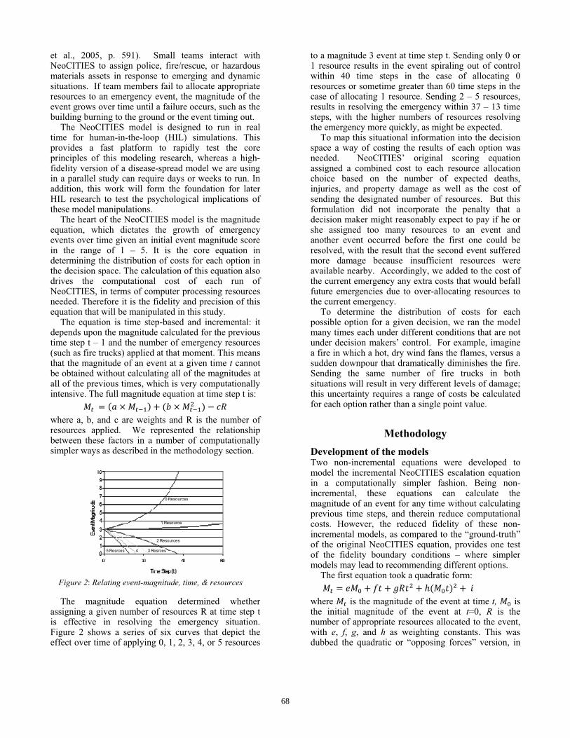
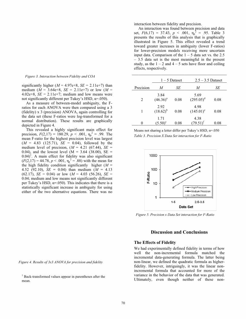
2= .001) with low fidelity having a higher mean cost (M = 53694.58, SE = 267.19) than medium (M = 52335.50, SE = 266.84) or high (M = 51801.30, SE = 266.24; medium and high means were not significantly different per Tukey’s HSD, �=.050). An interaction was found between fidelity and course of action, shown in Figure 3 (F(10,20943) = 8.38, p < .001, �p

2= .004). The high-fidelity model shows greater differentiation

between the mean costs associated with each course of action than the medium or low fidelity models. This was confirmed by analyzing the variances associated with each combination of fidelity and precision using a 3 (fidelity) x 3 (precision) ANOVA, controlling for the data set. A main effect for fidelity on variance was highly significant (F(2,24) = 10.48, p < .001, �p

2 = .47) with the mean variance for the high fidelity condition

69

sm4n

r(thnd

pm(m00(th4(0pse

1 m

Fig

significantly himedium (M = 4.02e+8, SE = not significantly

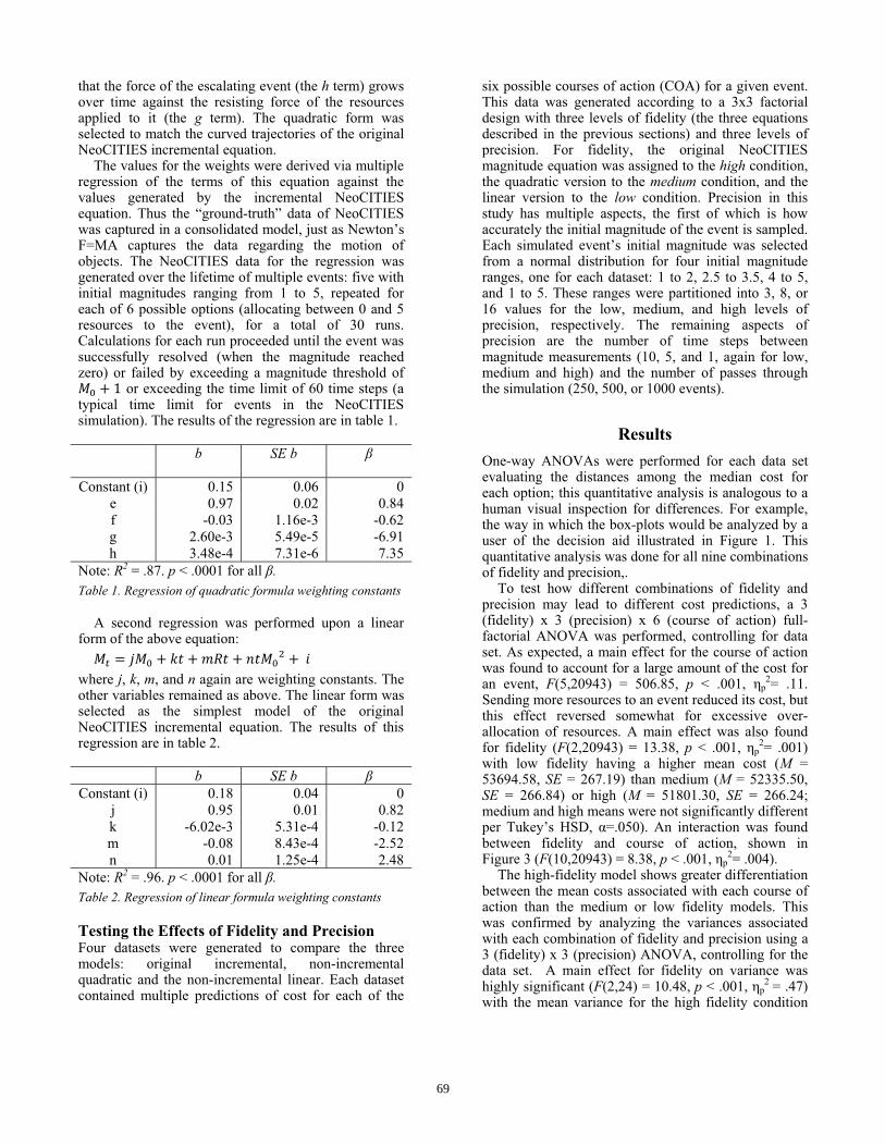
As a measuratios for each fidelity) x 3 (phe data set (th

normal distribdepicted in Figu

This revealeprecision, F(2,mean F-ratio foM = 4.83 (1

medium level 0.04), and the 0.04)1. A mainF(2,17) = 44.7he high fidelit

4.52 (92.10), 62.17), SE =

0.04; medium aper Tukey’s HSstatistically sigeither of the tw

Back-transform

mean.

gure 4. Results of

Figure 3. Inter

igher (M = 4.93.64e+8, SE 2.11e+7; med

y different per ure of between

ANOVA wereprecision) ANOhese F-ratios wbution). Theseure 4. ed a highly si17) = 180.29,or the highest p125.71), SE =of precision, lowest level

n effect for fid78, p < .001, �pty condition sSE = 0.04) t0.04) or low

and low meansSD, �=.050). Tgnificant increawo alternative

med values appea

f 3x3 ANOVA fo

raction between

97e+8, SE = 2.= 2.11e+7) o

dium and low Tukey’s HSD

n-model ambige then comparOVA, again cowere log-transfe results are

ignificant mai p < .001, �p

2

precision level= 0.04), follow(M = 4.21 (6(M = 3.64 (3

delity was alsop

2 = .88) with tsignificantly hthan medium (M = 4.03 (5

s not significanThis indicates thase in ambiguie equations. Th

ar in parentheses

or precision and f

Fidelity and CO

.11e+7) than or low (M =

means were D, �=.050). guity, the F-ed using a 3

ontrolling for formed for a

graphically

in effect for 2 = .99. The l was largest wed by the

67.44), SE = 8.00), SE = o significant the mean for higher (M =

(M = 4.13 56.26), SE = ntly different hat there is a ity for using here was no

s after the

fidelity

OA

int

setpreillutowforinp– stueff

Pr

MeTab

ThWeweincnofidincvarUl

F

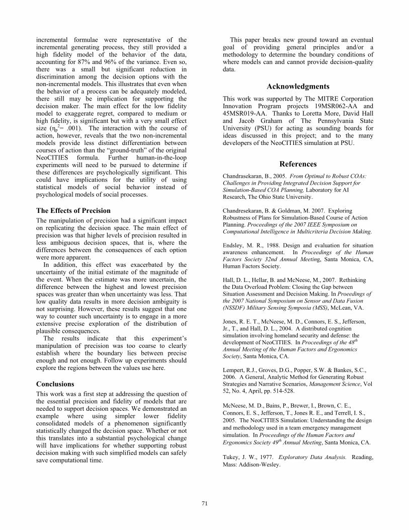
teraction betweAn interactiont, F(6,17) = 3esents the resuustrated in Fiward greater inr lower-precisiput data. Comp3.5 data set i

udy, as the 1 –fects, respectiv

recision M

2 3.8

(46.3

1 2.9

(18.6

0 1.7

(5.5

eans not sharing ble 3. Precision

Discu

he Effects of e had experimeell the non-cremental datan-linear, we de

delity. Howevecremental formriance in the btimately, eve

Figure 5. Precisio

een fidelity andn was found be37.43, p < .0ults of this anagure 5. This ncreases in amion models reparison of the s the most m2 and 4 – 5 se

vely.

1 – 5 Dataset

M SE

84 36)a 0.08

92 62)b 0.08

71 50)c 0.08

a letter differ peX Data Set inter

ussion and C

Fidelityentally defined-incremental a-generating foefined the quaer, intriguinglymula that accobehavior of the en though n

on x Data Set int

d precision. etween precisio001, �p

2 = .95alysis that is geffect reveale

mbiguity (loweeceiving more1 – 5 data set eaningful in tets have floor a

2.5 – 3.

M

5.69 (295.05)d

4.98 (145.01)e

4.38 (79.51)f

er Tukey’s HSDraction for F-Ra

Conclusions

d fidelity in terformula mat

ormula. The ladratic formula

y, it was the lounted for mo data that was

neither of th

teraction for F-R

on and data 5. Table 3 graphically ed a trend er F-ratios) e uncertain vs. the 2.5

the present and ceiling

5 Dataset

SE

0.08

0.08

0.08

, �=.050 atio

s

rms of how tched the atter being as higher-linear non-ore of the generated.

hese non-

Ratio

70

incremental formulae were representative of the incremental generating process, they still provided a high fidelity model of the behavior of the data, accounting for 87% and 96% of the variance. Even so, there was a small but significant reduction in discrimination among the decision options with the non-incremental models. This illustrates that even when the behavior of a process can be adequately modeled, there still may be implication for supporting the decision maker. The main effect for the low fidelity model to exaggerate regret, compared to medium or high fidelity, is significant but with a very small effect size (�p

2= .001). The interaction with the course of action, however, reveals that the two non-incremental models provide less distinct differentiation between courses of action than the “ground-truth” of the original NeoCITIES formula. Further human-in-the-loop experiments will need to be pursued to determine if these differences are psychologically significant. This could have implications for the utility of using statistical models of social behavior instead of psychological models of social processes.

The Effects of Precision The manipulation of precision had a significant impact on replicating the decision space. The main effect of precision was that higher levels of precision resulted in less ambiguous decision spaces, that is, where the differences between the consequences of each option were more apparent.

In addition, this effect was exacerbated by the uncertainty of the initial estimate of the magnitude of the event. When the estimate was more uncertain, the difference between the highest and lowest precision spaces was greater than when uncertainty was less. That low quality data results in more decision ambiguity is not surprising. However, these results suggest that one way to counter such uncertainty is to engage in a more extensive precise exploration of the distribution of plausible consequences.

The results indicate that this experiment’s manipulation of precision was too coarse to clearly establish where the boundary lies between precise enough and not enough. Follow up experiments should explore the regions between the values use here.

Conclusions This work was a first step at addressing the question of the essential precision and fidelity of models that are needed to support decision spaces. We demonstrated an example where using simpler lower fidelity consolidated models of a phenomenon significantly statistically changed the decision space. Whether or not this translates into a substantial psychological change will have implications for whether supporting robust decision making with such simplified models can safely save computational time.

This paper breaks new ground toward an eventual goal of providing general principles and/or a methodology to determine the boundary conditions of where models can and cannot provide decision-quality data.

Acknowledgments This work was supported by The MITRE Corporation Innovation Program projects 19MSR062-AA and 45MSR019-AA. Thanks to Loretta More, David Hall and Jacob Graham of The Pennsylvania State University (PSU) for acting as sounding boards for ideas discussed in this project; and to the many developers of the NeoCITIES simulation at PSU.

References Chandrasekaran, B., 2005. From Optimal to Robust COAs: Challenges in Providing Integrated Decision Support for Simulation-Based COA Planning, Laboratory for AI Research, The Ohio State University. Chandresekaran, B. & Goldman, M. 2007. Exploring Robustness of Plans for Simulation-Based Course of Action Planning. Proceedings of the 2007 IEEE Symposium on Computational Intelligence in Multicriteria Decision Making. Endsley, M. R., 1988. Design and evaluation for situation awareness enhancement. In Proceedings of the Human Factors Society 32nd Annual Meeting, Santa Monica, CA, Human Factors Society. Hall, D. L., Hellar, B. and McNeese, M., 2007. Rethinking the Data Overload Problem: Closing the Gap between Situation Assessment and Decision Making. In Proeedings of the 2007 National Symposium on Sensor and Data Fusion (NSSDF) Military Sensing Symposia (MSS), McLean, VA. Jones, R. E. T., McNeese, M. D., Connors, E. S., Jefferson, Jr., T., and Hall, D. L., 2004. A distributed cognition simulation involving homeland security and defense: the development of NeoCITIES. In Proceedings of the 48th Annual Meeting of the Human Factors and Ergonomics Society, Santa Monica, CA. Lempert, R.J., Groves, D.G., Popper, S.W. & Bankes, S.C., 2006. A General, Analytic Method for Generating Robust Strategies and Narrative Scenarios, Management Science, Vol 52, No. 4, April, pp. 514-528. McNeese, M. D., Bains, P., Brewer, I., Brown, C. E., Connors, E. S., Jefferson, T., Jones R. E., and Terrell, I. S., 2005. The NeoCITIES Simulation: Understanding the design and methodology used in a team emergency management simulation. In Proceedings of the Human Factors and Ergonomics Society 49th Annual Meeting, Santa Monica, CA. Tukey, J. W., 1977. Exploratory Data Analysis. Reading, Mass: Addison-Wesley.

71