supporting information -...

Supporting InformationFerguson et al. 10.1073/pnas.1003293107SI TextDiffusion Map. Given a set of N points in n-dimensional space,f ~xigNi¼1, ~xi ∈ Rn, the diffusion map approach seeks to constructthe “best” k-dimensional embedding of the data, where clarifica-tion of best will be briefly deferred. In the current work, the f ~xigcorrespond to the N 3R-dimensional snapshots of the simulationtrajectory recording the coordinates of all R atoms in the system.A scalar-valued similarity metric between pairs of data pointsproviding a locally, but not necessarily globally, meaningful mea-sure of dynamic proximity is used to establish the local connec-tivity of each data point on the intrinsic manifold. The diffusionmap fuses this local structural information into a global descrip-tion of the manifold (1).

Although a number of choices of similarity metric are possible,we selected the rotationally and translationally minimized rmsdbetween the coordinates of the n-alkane united atom centers (2).Although this measure does not explicitly consider solvent de-grees of freedom, the solvent influences the simulation trajectoryand its effect is therefore “encoded” in the hydrocarbon config-urations sampled. In the absence of an easily calculable dynamicmeasure of proximity, we consider this structural metric a goodsurrogate. A Gaussian kernel of bandwidth ϵ > 0 is then appliedto the pairwise rmsd values to specify the locale within which thesimilarity metric is considered meaningful and imbue the diffu-sion map with useful mathematical properties (1, 3, 4), to yieldthe real, symmetric, N-by-N pairwise similarity matrix

Aij ¼ exp�−ðrmsdijÞ2

2ϵ

�i; j ¼ 1;…;N:

As an example calculation, Fig. S1 provides a log–log plot of∑i;jAij versus ϵ for the solvated C16 system. Using the correlationdimension as a measure of fractal dimensionality as introduced byGrassberger and Procaccia (5), Coifman et al. (1) have shown thelinear region of such plots to delimit the range of appropriate ϵvalues, and twice its slope to provide an estimate of the intrinsicdata dimensionality.

A diagonal matrix D is constructed from the row sums of Aand combined with A to construct a right stochastic Markovtransition matrix M, where Mij may be interpreted as transitionprobability of hopping from data point i to data point j in a “timestep” Δt ¼ ϵ (6),

Dii ¼ ∑N

j¼1

Aij i ¼ 1;…;N;

M ¼ D−1A:

The Markov transition matrix is closely related to the normalizedgraph Laplacian L ¼ I −M, where I is the identity matrix and, inthe limit of N → ∞ and ϵ → 0, converges to the backwardFokker–Plank (FP) operator describing a continuous diffusionprocess in the presence of potential wells (1),

LFPþ ¼ ΔLB − 2∇UðxÞ · ∇;

where ΔLB is the Laplace–Beltrami operator over the manifold(a generalization of the Laplacian to functions defined onsurfaces), and UðxÞ ¼ − log pðxÞ, where pðxÞ is the density of data

points on the manifold. The steady-state solution of the corre-sponding forward FP equation is given by the Boltzmann distribu-tion pðx;t ¼ ∞Þ ¼ Z−1e−UðxÞ, where Z is a normalizing partitionfunction and UðxÞ may be regarded as a free energy (3). Freeenergy surfaces (FES) may be computed from histogram approx-imations of pðxÞ.

Because M is adjoint to a symmetric matrix MS ¼ D12MD−1

2,positive-semidefinite and right stochastic, its ordered eigenvaluesfλigNi¼1, λ1 ≥ λ2 ≥ ⋯λN lie on the interval ð0;1�, the associated realeigenvectors f ~ϕigNi¼1 are orthogonal and the top eigenvector istrivial with λ1 ¼ 1 and ~ϕ1 ¼ ~1. The k-dimensional diffusionmap is an embedding of the N n-dimensional data points intothe components of the data in the top nontrivial k < n ≪ Neigenvectors (3, 4, 6),

~xi ↦ ð ~ϕ2ðiÞ; ~ϕ3ðiÞ;…; ~ϕkþ1ðiÞÞ;which may be computed as described in Materials and Methods.For brevity, this mapping will henceforth be referred to simply asthe “embedding in the top k eigenvectors.”

The symmetric matrix MS is diagonalized into the real, diag-onal matrix of its eigenvalues Λ by the orthogonal matrix V, thecolumns of which are its eigenvectors,

MS ¼ D12MD−1

2 ¼ VΛVT

⇒ M ¼ D−12VΛVTD

12 ¼ ΦΛΨT

⇒ Mij ¼ ∑N

p¼1

~ϕpðiÞλp ~ψpðjÞ:

Ψ ¼ D12V ¼ f ~ψ igNi¼1 and Φ ¼ D−1

2V ¼ f ~ϕigNi¼1 are the left andright column eigenvectors ofM, respectively, and form a biortho-gonal set, ΨTΦ ¼ 1. M raised to the qth power is thereforegiven by

Mq ¼ ΦΛqΨT ⇒ Mij ¼ ∑N

p¼1

~ϕpðiÞλqp ~ψpðjÞ:

Following refs. 3 and 6, we define the squared diffusion distancebetween data points i and j as a function of q as

D2qði;jÞ ¼ ∑

N

k¼1

ðMqik −Mq

jkÞ2Dkk

:

ConsideringMij as the probability of hopping from i to j in a finitetime step Δt ¼ ϵ, and assuming this jump process to be Marko-vian (6), allowsMq

ij to be interpreted as the probability of hoppingfrom i to j in time qΔt. Accordingly,D2

qði;jÞmeasures the squareddifference between the probability of diffusing from point i topoint k and the probability of diffusing from point j to point kafter time qΔt (i.e., after q applications of the Markov matrixM) summed over all k ¼ 1;…;N data points. Dkk is a normalizingfactor which accounts for the local density of data points (6). Dq

may therefore be viewed as a measure of the overlap of the twoprobability distributions initially centered on point i and point j(6), and will be small if there are a large number of short pathsconnecting i and j (3). Expanding out the right-hand side,

Ferguson et al. www.pnas.org/cgi/doi/10.1073/pnas.1003293107 1 of 10

http://www.pnas.org/cgi/doi/10.1073/pnas.1003293107

D2qði;jÞ ¼ ∑

N

k¼1

1

Dkk

�∑N

p¼1

~ϕpðiÞλqp ~ψpðkÞ −∑N

p¼1

~ϕpðjÞλqp ~ψpðkÞ�

2

¼ ∑N

k¼1

1

Dkk

�∑N

p¼1

ðλqp ~ϕpðiÞ − λqp ~ϕpðjÞÞ ~ψpðkÞ�

2

¼ ∑N

k¼1

1

Dkk ∑N

p¼1

ðλqp ~ϕpðiÞ − λqp ~ϕpðjÞÞ2 ~ψpðkÞ2

¼ ∑N

p¼1

ðλqp ~ϕpðiÞ − λqp ~ϕpðjÞÞ2 ∑N

k¼1

~ψpðkÞ2Dkk

¼ ∑N

p¼1

ðλqp ~ϕpðiÞ − λqp ~ϕpðjÞÞ2;

where relationships following from the orthogonality of V,

VTV ¼ ΨTD−12D−1

2Ψ ¼ 1

⇒ ∑N

k¼1

~ψpðkÞ ~ψpðkÞDkk

¼ 1

and ∑N

k¼1

~ψpðkÞ ~ψqðkÞDkk

¼ 0

are used to eliminate cross-terms in expanding out line two toobtain line three, and in going from line four to line five. Selectingq ¼ 0 to obtain the diffusion distance in the zero time limit (6),

D20 ¼ ∑

N

p¼1

ð ~ϕpðiÞ − ~ϕpðjÞÞ2:

This expression demonstrates that theEuclidean distance betweentwo points in a diffusion map embedding comprising all (N − 1)nontrivial eigenvectors is identical to the q ¼ 0 diffusion distancebetween the points. (Taking q ¼ 0may seem to suggest a diffusionprocess with zero steps, but diffusion distances within the localizedregion of each data point are built into the M matrix by its con-struction from pairwise distances combined with a Gaussian ker-nel. In a sense, therefore, the q ¼ 0 limit corresponds to a processwhich has already taken a single diffusion step.) Points which aredynamically proximate (i.e., connected by a large number of shortpathways) are situated close together in the diffusion map embed-

ding. In practice, for reducible systems, good approximations ofDq are provided by embeddings in the top few eigenvectors (3).

The eigenvectors f ~ϕigNi¼1 are discrete approximations to thetop eigenfunctions ϕiðxÞ of the backward FP operator, withcorresponding eigenvalues σi, σ1 ¼ 0 ≥ σ2 ≥ ⋯ (1). The spectralsolution of the backward FP equation is (3)

pðx;tÞ ¼ ∑∞

i¼1

cie−σi tϕiðxÞ;

where the ci coefficients are determined by the initial state. Be-cause the long-time behavior is dictated by the top few eigenfunc-tions, an embedding in the top eigenvectors captures the slowdynamics of the system, and is termed the “intrinsic” or “slow”manifold.

This dynamically meaningful interpretation of the diffusionmap embedding rests on two assumptions. Firstly, it is assumedthat the dynamics of the systemmay be well modeled as a diffusionprocess. For biophysical systems expected to exhibit low effectivedimensionalities due to cooperative couplings between degrees offreedom (7–11), this is expected to be a good assumption, becausethe projection operator approach (12) permits the dynamics to beformulated in a coarse-grained manner as a set of stochasticdifferential equations describing the evolution of the small num-ber of slow variables, with the stochastic noise arising from thedynamics of the remaining fast degrees of freedom. Secondly,the scalar-valued pairwise similaritymetric is assumed to be a goodlocal descriptor of the short-time diffusive motions. For molecularsystems, the diffusive motions arising from the fast degrees offreedom are manifested as “thermal noise” in the slow variablesand are expected to be captured by a structural similarity metric,such as the rotationally and translationally minimized rmsdemployed in this work. If both of these assumptions are satisfied,then pathways over the diffusion map embedding describe theevolution of the system in its fundamental dynamical motions.Even if either assumption does not hold, the diffusion mapapproach is still robust in the sense that, although the identifiedorder parameters may no longer be considered to capture the truefundamental dynamics, they remain good variables with which toparametrize the transitions of the system from one state toanother. To objectively verify whether the order parametersfurnished by the diffusion map are truly dynamically relevantwould require a subsequent computationally intensive evaluationof committor probabilities along the pathway by, for example,transition path sampling (13).

1. Coifman RR, Shkolnisky Y, Sigworth FJ, Singer A (2008) Graph laplacian tomographyfrom unknown random projections. IEEE T Image Process 17:1891–1899.

2. Maiorov VN, Crippen GM (1995) Size-independent comparison of protein three-dimensional structures. Proteins 22:273–283.

3. Coifman RR, et al. (2005) Geometric diffusions as a tool for harmonic analysis andstructure definition of data: Diffusion maps. Proc Natl Acad Sci USA 102:7426–7431.

4. Belkin M, Niyogi P (2003) Laplacian eigenmaps for dimensionality reduction and datarepresentation. Neural Comput 15:1373–1396.

5. Grassberger P, Procaccia I (1983) Measuring the strangeness of strange attractors.Physica D 9:189–208.

6. Nadler B, Lafon S, Coifman RR, Kevrekidis I (2006) Advances in Neural InformationProcessing Systems 18, eds Weiss Y, Schölkopf B, Platt J (MIT Press, Cambridge, MA)pp 955–962.

7. García AE (1992) Large-amplitude nonlinear motions in proteins. Phys Rev Lett68:2696–2699.

8. Amadei A, Linssen ABM, Berendsen HJC (1993) Essential dynamics of proteins. Proteins17:412–425.

9. Hegger R, Altis A, Nguyen PH, Stock G (2007) How complex is the dynamics of peptide

folding? Phys Rev Lett 98:028102-028104.

10. Zhuravlev PI, Materese CK, Papoian GA (2009) Deconstructing the native state:

Energy landscapes, function, and dynamics of globular proteins. J Phys Chem B

113:8800–8812.

11. Das P, Moll M, Stamati H, Kavraki LE, Clementi C (2006) Low-dimensional, free-energy

landscapes of protein-folding reactions by nonlinear dimensionality reduction. Proc

Natl Acad Sci USA 103:9885–9890.

12. Zwanzig R (2001) Nonequilibrium Statistical Mechanics (Oxford Univ Press, New York)

pp 143–168.

13. Miller TF, Vanden-Eijnden E, Chandler D (2007) Solvent coarse-graining and the string

method applied to the hydrophobic collapse of a hydrated chain. Proc Natl Acad Sci

USA 104:14559–14564.

14. Humphrey W, Dalke A, Schulten K (1996) VMD—visual molecular dynamics. J Mol

Graphics 14:33–38.



Fig. S1. A log–log plot of the sum of the elements of the pairwise similarity matrix,∑i;jAij , as a function of the Gaussian kernel bandwidth, ϵ, for the solvatedphase C16 system. The linear region delineates the range of suitable ϵ values and twice its slope provides an estimate of the effective dimensionality. A value ofϵ ¼ 0.002 was selected, and the effective dimensionality was estimated to lie between 3.9 and 5.6, where the spread arises from the precise location at whichthe slope is computed.

Fig. S2. The principal moments of the n-alkane gyration tensor ðξ1;ξ2;ξ3Þ serve as useful intermediary variables in the interpretation of the order parametersidentified by the diffusion map. (A, B) Diagonalization of the n-alkane gyration tensor corresponds to the adoption of a coordinate reference frame in whichthe three principal moments (square roots of the eigenvalues of the gyration tensor) describe the characteristic length of the n-alkane chain along the threemutually orthogonal principal axes. A schematic illustration provides a physical interpretation of ðξ1;ξ2;ξ3Þ for a particular conformation of C16. (C) A replottingof Fig. 1A (a two-dimensional elevation of the three-dimensional embedding of the solvated phase C8 system in evec2, evec3, and evec4) with the data pointsnow colored according to Rg rather than ξ1. (D) For molecules with high aspect ratios such as n-alkane chains, ξ1 is much greater than ξ2 or ξ3 for most chainconformations and is the dominant contribution to R2

g ¼ ξ21 þ ξ22 þ ξ23. Accordingly, ξ1 and Rg are highly correlated, and the mapping between them approxi-mately bijective, as illustrated here for the solvated phase C8 system.



Fig. S3. Two-dimensional elevations of the three-dimensional embedding of the ideal-gas phase C8 system in evec2, evec3, and evec4. Data points are coloredaccording to the (A) first and (B) third principal moments of the gyration tensor.

Fig. S4. FES of the ideal-gas phase C8 system embedded in evec2, evec3, and evec4 with representative chain conformations. Molecules are oriented so thatthe head is farther from the reader. The range of βG is 2.8–10.3, with isosurfaces plotted at βG ¼ 5, 6, 7, and 8. The ninth low-ξ3 region midway betweenstructures 2 and 3 has not been associated with a distinct chain structure, because it describes transitory conformations between these two structures contain-ing gauche defects in both the head and tail.



Fig. S5. Eigenvector component functional dependency in the solvated phase C16 system. (A) A two-dimensional embedding of the solvated phase C16 systemin evec2 and evec3. The functional dependency between the order parameters associated with the components of these eigenvectors is manifested as acollapse of the intrinsic manifold onto an essentially one-dimensional curve. (B) Two piecewise continuous quartic functions were fitted to the curve in(A) and the arclength calculated by numerical integration. The origin from which arclength is measured is arbitrary, but in this case corresponds approximatelyto the location of the high ξ1 tip at (evec2 ¼ 0.001, evec3 ¼ −0.006). This plot illustrates the bijective mapping between evec2 and arclength. Parametrizationof the one-dimensional curve in A by arclength can be conceptualized as “straightening out” the curve in evec2–evec3 space.



Fig. S6. Two-dimensional elevations of the three-dimensional embedding of the solvated phase C16 system in evec2/3 arclength, evec4, and evec6. Evec5 wasobserved to have a functional dependence on arclength, and was rejected in favor of evec6 in the construction of the embedding; the associated eigenvaluesare spectrally close. Data points are colored according to the (A) first, (B) second, and (C) third principal moments of the C16 gyration tensor. Molecules areoriented such that the head is farther from the reader, and solvent has been removed for clarity. Although both are constructed from 30,001 snapshots, thedensity of points in this embedding may appear sparser than the corresponding solvated phase C24 embedding (Fig. 3) because a larger proportion of the C16

points reside in the densely populated low-arclength region.



Fig. S7. Two-dimensional elevations of the three-dimensional embedding of the ideal-gas phase C16 system in evec2/3 arclength, evec5, and evec6. Evec4 wasobserved to have a functional dependence on arclength, and was rejected in favor of evec6 in the construction of the embedding; the associated eigenvaluesare spectrally close. Data points are colored according to the (A) first, (B) second, and (C) third principal moments of the C16 gyration tensor. Molecules areoriented such that the head is farther from the reader. Although both are constructed from 30,001 snapshots, the density of points in this embedding mayappear sparser than the corresponding ideal-gas phase C24 embedding (Fig. S8) because a larger proportion of the C16 points reside in the densely populatedlow-arclength region.



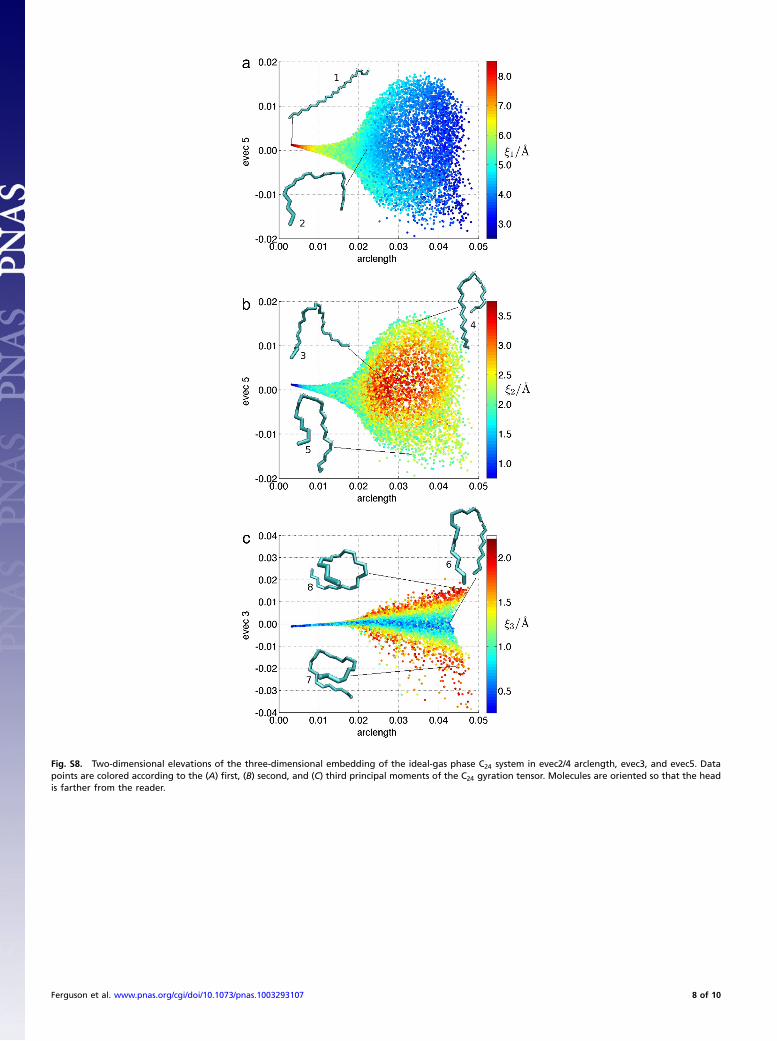
Fig. S8. Two-dimensional elevations of the three-dimensional embedding of the ideal-gas phase C24 system in evec2/4 arclength, evec3, and evec5. Datapoints are colored according to the (A) first, (B) second, and (C) third principal moments of the C24 gyration tensor. Molecules are oriented so that the headis farther from the reader.



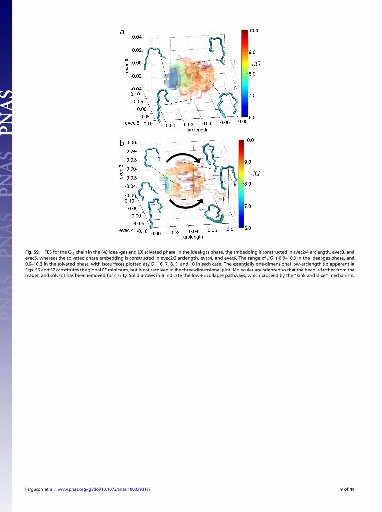
Fig. S9. FES for the C16 chain in the (A) ideal-gas and (B) solvated phase. In the ideal-gas phase, the embedding is constructed in evec2/4 arclength, evec3, andevec5, whereas the solvated phase embedding is constructed in evec2/3 arclength, evec4, and evec6. The range of βG is 0.9–10.3 in the ideal-gas phase, and0.6–10.3 in the solvated phase, with isosurfaces plotted at βG ¼ 6, 7, 8, 9, and 10 in each case. The essentially one-dimensional low-arclength tip apparent inFigs. S6 and S7 constitutes the global FE minimum, but is not resolved in the three-dimensional plot. Molecules are oriented so that the head is farther from thereader, and solvent has been removed for clarity. Solid arrows in B indicate the low-FE collapse pathways, which proceed by the “kink and slide” mechanism.



Movie S1. A continuous 200 ps portion of the 30 ns solvated phase C24 molecular dynamics trajectory showing the spontaneous collapse and reextension ofthe n-alkane chain, visualized using Visual Molecular Dynamics (14). The united atoms constituting the C24 chain are represented as van der Waals spheres ofradius 1.7 Å, and are colored light blue. The solvent excluded cavity containing the n-alkane is defined as that volume bounded by the surface generated byrolling a spherical probe of radius 2.3 Å over the solvent molecules surrounding the n-alkane chain; this bounding surface is colored purple. The algorithm usedto render the excluded cavity volume surface also detects the walls of the periodic simulation box and naturally occurring cavities in the bulk solvent sufficientlylarge to accommodate the probe. The simulation boxwalls are visible in the background, and cavities in the bulk are observed in a number of frames. The proberadius was selected to be as small as possible without detecting so many cavities in the bulk solvent so as to obscure the n-alkane chain. To facilitate visualiza-tion of the chain dynamics, the internal motions of the n-alkane chain were decoupled from the center of mass motion by rotationally and translationallyfitting each frame of the video to the initial frame. Accordingly, the walls of the simulation box appear to move around behind the hydrocarbon chain.

The C24 molecule is initially in an extended conformation, with the solvent excluded volume wrapped tightly around its length. A bend then develops in thecenter of the chain, and it adopts a loose, symmetric hairpin conformation. The region between the arms of the hairpin remains hydrated, as evinced by theboundary of the solvent excluded volume, which remains close to the surface of the van der Waals spheres and does not extend into this region. A kink thendevelops near the head of the chain from which the solvent is expelled, and the solvent excluded volume coalesces to encompass the n-alkane atoms on eachside of the bend. The kink slides down the length of the chain, accompanied by the gradual expulsion of solvent from the interior region between the arms ofthe chain. The molecule then adopts a tight, symmetric hairpin conformation with a dry interior, with the solvent excluded volume fully encompassing botharms of the chain. The chain further collapses into a right-handed helical coil with a dry core.

Having completely collapsed, the chain reextends by retracing its collapse pathway in the opposite direction. The helical coil first opens out into a symmetrichairpin with a dry interior, followed by the migration of the kink toward the head of the chain, accompanied by rehydration of the tail region residing out withthe bend. Finally, the kink at the head of the chain dissolves with the ingress of solvent, and the chain readopts an extended state.

The chain collapse and reextension events follow the kink and slide mechanism, and the states of the chain along the pathway are well characterized by thethree global order parameters identified by the diffusionmap approach: degree of chain collapse, location of the bend in the chain, and the handedness of thechain helicity.

Movie S1 (MPG)


http://www.pnas.org/lookup/suppl/doi:10.1073/pnas.1003293107/-/DCSupplemental/SM01.mpg


supporting information -...

Documents