www.sciencemag.org/cgi/content/full/325/5941/710/DC1

Supporting Online Material for

The Last Glacial Maximum

Peter U. Clark,* Arthur S. Dyke, Jeremy D. Shakun, Anders E. Carlson, Jorie Clark, Barbara Wohlfarth, Jerry X. Mitrovica, Steven W. Hostetler, A. Marshall McCabe

*To whom correspondence should be addressed. E-mail: clarkp@onid.orst.edu

Published 7 August 2009, Science 325, 710 (2009)

DOI: 10.1126/science.1172873

This PDF file includes

Materials and Methods SOM Text Figs. S1 to S5 References

Supporting Online Material 1172873s

Materials and Methods

Sea-Level Predictions. We predict relative sea-level (RSL) change at Barbados, New Guinea, Tahiti, Sunda Shelf and Bonaparte Gulf (Fig. S1) using a state-of-the-art theory that incorporates time varying shoreline geometry and the feedback of rotation onto sea level (1). The calculations are performed using the pseudo-spectral algorithm described in (1), with a truncation at spherical harmonic degree and order 256. The predictions are generated using an ice model adapted from (2) to include a realistic glaciation phase while at the same time retaining the excellent fits to post-LGM RSL curves obtained in that earlier study. Our ice model assumes that LGM begins at 26 ka, and it is characterized by a peak eustatic sea level fall of ~130m over the LGM period. The Earth model used in the calculations is the preferred model of (2); it includes an elastic lithosphere of 95 km, upper mantle viscosity of 5x1020 Pa s, and lower mantle viscosity of 4x1022 Pa s.

Our predictions highlight the important point that GIA will introduce a spatially varying component into post-glacial sea-level change, and the difference in the predictions at Barbados versus the other sites reflects an interesting aspect of the physics of GIA. At sites within the far-field of the late Pleistocene ice sheets during a period of relative ice sheet stability (e.g., the LGM period and interglacials), the GIA signal will be dominated by three effects. First, for sites such as Barbados, which lie at the outer flank of the peripheral bulge surrounding areas of glaciation, sea level is perturbed by the deformation of the solid Earth (uplift and sea-level fall during glaciation and LGM periods, subsidence and sea-level rise during deglaciation and interglacials). Second, the displacement of water due to the integrated adjustment of the various peripheral bulges also causes a global scale sea-level change. During deglaciation and interglacial periods this process, whereby water moves into regions being vacated by subsiding bulges, leads to a global scale sea-level fall (of order m/kyr) which has come to be known as ocean syphoning (3, 4); syphoning is responsible, for example, for the development of sea-level highstands at far-field island sites during the current interglacial. Interestingly, during glaciation and LGM periods the process acts in reverse, and uplifting bulges will push water outward and raise sea level globally. We will term this process, which has not previously been discussed in the literature, “anti-syphoning.” Finally, for sites near the vicinity of continental margins, ocean loading will tend to flex the lithosphere at such margins in a process called continental levering (5). Levering will induce a sea-level rise offshore and fall onshore during deglaciation and interglacial periods (order m/kyr), and the reverse during glaciation and LGM phases.

As a final point, we note that the relative sizes of the various GIA processes acting during the LGM will be dependent on the adopted model for the Earth's viscosity. As a consequence, the dominance of the peripheral bulge and levering signal during LGM at Barbados (Fig. S1) will not be a feature of all GIA predictions. As an example, the ICE-5G/VM2 model of (6) predicts a less extensive peripheral bulge surrounding Laurentia, and in this case the calculated RSL and ESL curves track each other during the LGM. This sensitivity to Earth structure means that Barbados RSL data will not in general be an uncontaminated measure of the ESL curve and excess ice volume at LGM (7).

Figure S1. Sea-level predictions for New Guinea (solid sky-blue line), Barbados (solid blue line), Tahiti (solid green line), Bonaparte Gulf (dashed green line), and Sunda Shelf (dashed sky-blue line) compared to relative sea-level (RSL) data with depth uncertainty for the interval 10-30 ka from New Guinea (sky-blue circles) (32-34), Barbados (blue triangles) (35, 36), Bonaparte Gulf (green half-pluses representing age and depth uncertainty) (37), Sunda Shelf (sky-blue half-pluses) (38), and Tahiti (39). Eustatic sea-level time series shown as gray line.

30 20 10Age (ka)

-150

-125

-100

-75

-50

RSL

(m)

Geochronological Constraints on Ice-Sheet and Glacier Maxima. We apply well-established conventions for using published 14C and TCN ages to constrain ice-margin fluctuations. 14C ages are largely obtained from organic matter that occurs stratigraphically beneath or above glacial deposits from an ice-margin fluctuation. Accordingly, these dates only provide limiting maximum and minimum ages that bracket the duration of the fluctuation but leave some uncertainty in the exact timing of advance and retreat. In many cases, however, stratigraphic relationships document that the ages are in fact closely recording the timing of the fluctuation (e.g., proglacial lake dammed by ice margin, marine sediments deposited in isostatically depressed basins, sheared sediments with organics indicating near-contemporaneous overriding of site by ice). Moreover, our large data base often includes multiple limiting ages from a given region that - when in good agreement - closely constrain the ice-margin fluctuation. In view of these considerations, we use the large number of limiting 14C ages and their well-established stratigraphic context to assign uncertainties to the beginning and end of regional ice-sheet maxima (Fig. S2, S3).

We calibrated 4443 14C ages using CALIB (8) ver. 5.02 for ages <24 14C ka , and the Fairbanks calibration for ages >24 14C ka (9). Appropriate reservoir ages are assigned to all marine samples. We carefully assessed all 14C ages for integrity, and any ages on unreliable

68 64 60 56 52Latitude (oN)

0 4 8 12Longitude (oE)

60 64 68 72Latitude (oN)

50

40

30

20

10

Age

(ka)

-160 -150 -140Longitude (oW)

-140 -130 -120 -110Longitude (oW)

50

40

30

20

10

Age

(ka)

-138 -132 -126Longitude (oW)

1000 500 0Distance (km)

50

40

30

20

10

Age

(ka)

800 400 0Distance (km)

48 46 44 42Latitude (oN)

-68 -64 -60 -56Longitude (oW)

50

40

30

20

10A

ge (k

a)

1000 500 0Distance (km)

-120 -110 -100Longitude (oW)

-120 -100 -80 -60Longitude (oW)

a

e

i

m

b

f

j

n

c d

g h

k l

o p

? ???

ScIS

64 68 72Latitude (oN)

Figure S2. Compilation of 3419 14C ages and 375 TCN ages used to identify the time of the local last glacial maximum (LLGM) for various Northern Hemisphere ice-sheet sectors and ice sheets. Most ages are plotted in the direction of former ice flow (time-distance diagrams), with specific direction identified in the more detailed description of each plot below. Calibrated 14C ages are shown as 1σ range, with red symbols indicating ages that constrain there to be no ice at that time and location, and blue symbols are limiting (maximum or minimum) ages that are stratigraphically associated with evidence for ice at the site. Individual cosmogenic (10Be) surface exposure ages are shown as smaller light-gray circles, whereas the mean ages of individual ages associated with a single landform are shown as larger dark-gray circles, with associated error. The horizontal blue bars with gray bars above and below represent the time of the LLGM and associated error, respectively. (a) Time-distance diagram for the Maritimes region of the LIS. Because ice flow in this region was complex, as it included multiple outflow centers, there is no particular significance to the orientation of the x-axis. (b) Time-distance diagram for the New England sector of the LIS, with direction of flow from north to south. Pink triangles are deglaciation ages defined from the New England varve chronology (40). (c) Time-distance diagram for the Ohio-Erie-Ontario Lobe of the LIS, with direction of flow from northeast to southwest, and distance shown being distance from the terminal (Hartwell) moraine in Ohio. (d) Time-distance diagram for the Lake Michigan Lobe of the LIS, with direction of flow from north to south, and distance shown being the distance from the terminal (Shelbyville) moraine in Illinois. (e) Time-distance diagram for the Des Moines Lobe of the LIS, with direction of flow from north to south, and distance shown being distance from the terminal (Bemis) moraine in Iowa. (f) Time-distance diagram for the western sector of the LIS on the Canadian prairies, with direction of flow being approximately from east to west. In this case, there are no ages that closely constrain the termination of the LLGM of this sector of the LIS. (g) Time-distance diagram for the Mackenzie River Lobe of the LIS. Because direction of LGM ice flow was to the northwest, the orientation of the x-axis is oblique to ice flow. (h) Ages from the northeast sector of the LIS. In this case, the ages are plotted along a N-S transect that is oblique to ice flow, with most ages occurring on the east coast of Baffin Island. (i) Ages from the main sector of the Cordilleran Ice Sheet (CIS) that occurs <138oW. In this case, the ages are plotted along an E-W transect, but with no indication of ice-flow direction. The blue diamonds are calibrated 14C ages on organic material from the Quadra Sand, which was deposited as outwash sediments in advance of the growing ice sheet. A number of calibrated 14C ages are shown in blue as occurring well before the LLGM, but these are from organics in sediments associated with the growth of the ice sheet to its LLGM position. (j) Ages from the sector of the CIS that occur >138oW. In this case, the ages are plotted along an E-W transect, but with no indication of ice-flow direction. (k) Ages from the Innuitian Ice Sheet (IIS) that occur <138oW. In this case, the ages are plotted along an E-W transect, but with no indication of ice-flow direction. Calibrated 14C ages shown as the standard blue and red symbols are from the lowland sector of the ice sheet, whereas symbols in sky blue and light orange constrain ice presence and absence, respectively, from the alpine region of the ice sheet. (l) Ages from the British-Irish Ice Sheet (BIIS). In this case, ages are plotted first as those associated with the Irish Ice Sheet on the left and from the Scottish sector (ScIS) of the BIIS on the right. For each of these two regions, the ages are then separated with calibrated 14C ages indicating no ice on the left (red symbols), TCN ages constraining time of deglaciation in the middle, and calibrated limiting 14C ages on the right (blue symbols). No distance is implied. (m) Ages from the Barents-Kara Ice Sheet

(BKIS). In this case, the ages are separated with calibrated 14C ages indicating no ice on the left (red symbols), TCN ages constraining time of deglaciation in the middle, and calibrated limiting 14C ages on the right (blue symbols). No distance is implied. (n) Ages from the west-northwest sector of the Scandinavian Ice Sheet (SIS). In this case, the ages are plotted along a N-S transect that is oblique to ice flow, with most ages occurring on or near the west coast of Norway. Calibrated 14C ages shown in gray are from the published literature, but we have assigned them a lower reliability ranking based on the material dated (i.e., bulk organic matter). (o) Time-distance diagram for the southwestern sector of the SIS, with direction of flow east to west. (p) Time-distance diagram for the central and southern sector of the SIS, with direction of flow from north to south.

Figure S3. Compilation of 852 14C ages and 100 TCN ages used to identify the time of the local last glacial maximum (LLGM) for Antarctica and Greenland ice sheets. Calibrated 14C ages are shown as 1σ range, with red symbols indicating ages that constrain there to be no ice at that time and location, and blue symbols are limiting (maximum or minimum) ages that are stratigraphically associated with evidence for ice at the site. Individual TCN (10Be) ages are shown as smaller light-gray circles, whereas the mean ages of individual 10Be ages associated with a single landform are shown as larger dark-gray circles, with associated error. Individual 3He TCN ages are shown as sky-blue triangles. The horizontal blue bars with gray bars above and below represent the time of the LLGM and associated error, respectively. (a) Ages from the West Antarctic Ice Sheet (WAIS), Antarctic Peninsula Ice Sheet (APIS), and East Antarctic Ice Sheet (EAIS). All ages from APIS and EAIS (each outlined by gray-line boxes) are TCN ages on individual boulders. Only ages from WAIS provide sufficient constraints to define the LLGM, with the majority of these being from the Ross Sea region. The stratigraphic position of the three calibrated 14C ages shown as gray symbols is unclear. The blue-symbol calibrated 14C ages in the gray-line box labeled TVLmx are on organic matter (algae) in sediments associated with high lake levels in Taylor Valley that require the WAIS ice margin to be at its maximum extent. The blue-symbol calibrated 14C ages immediately to the right of the gray-line box are on organic matter associated with sediments that indicate an ice-margin near the mouth of Taylor Valley, but not at its maximum extent. (b) Ages from the western and eastern margins of the Greenland Ice Sheet (W GIS and E GIS, respectively). In this case, the ages are plotted along a N-S transect that is oblique to ice flow, with most ages occurring on or near the coast of Greenland. These data do not provide sufficient constraints to define the start or termination of the LLGM.

50

40

30

20

10

0

Age

(ka)

APIS EAIS

TVLmx

80 70 60Latitude (oN)

80 70 60

a b

W GIS E GISWAIS

materials or ages that were specifically questioned in the literature were either excluded or assigned a low ranking (10).

In contrast to 14C ages, ages derived from in situ-produced terrestrial cosmogenic nuclides (TCN ages) in boulders on glacial moraines and other landforms mark the time of ice-margin retreat but provide no information on time of ice-margin advance. Compared with the number of 14C ages, there are relatively few TCN ages constraining retreat from ice-sheet maxima (Fig. S2, S3). In those cases where both chronologies exist, however, they are in excellent agreement in constraining the timing of deglaciation (Fig. S2b, S2l, S2p) (11-13). By comparison, organic matter for 14C dating is poorly preserved in mountain-glacier moraines, but there are many opportunities for cosmogenic surface exposure dating. TCN ages thus provide the primary geochronological constraint for determining the deglaciation age of mountain glaciers from sites in western North America, Europe, Tibet, the tropics and subtropics, and the Southern Hemisphere (Fig. S4).

Of the 1261 published TCN ages used here, most (1197) are 10Be ages and the remainder are 3He ages. We report the published 3He ages, but we have recalculated all published 10Be data used here with the CRONUS-Earth (Cosmic Ray prOduced NUclide Systematics on Earth) calculator (14). There is typically some scatter in the distribution of the TCN ages from a single moraine, reflecting various possible geological uncertainties (e.g., prior exposure, erosion) that are difficult to detect in the field. (It is for this reason that we place lesser significance on age constraints based on single TCN ages.) We statistically evaluated each age population to identify outliers, and excluded them from calculating the mean age and standard error of the population (see below). The largest uncertainties lie in the production rate and the five possible scaling factors used in calculating a TCN age (14). In plotting 10Be data, we have used the Lal-Stone (St) scaling option, but we also evaluate sensitivity of our results to the four other scaling factors. Lastly, we designed a strategy to assess the age of regional deglaciation from the LLGM for the five regions of mountain glaciation that includes uncertainties in the age population, production rate and scaling factors (see below).

We use the error associated with the calibrated 14C age range (±1 σ) of limiting ages to define the error for the beginning or termination of the local last glacial maximum (LLGM). Given that these are limiting ages, this error assignment may still overestimate (underestimate) the onset (termination) of the LLGM. In some cases, the best limiting 14C age for establishing when a maximum ice limit was attained occurs some distance up-ice from the limit, thus adding some additional uncertainty. In most cases, however, there are additional limiting ages that suggest the assigned error is reasonable. In three cases (New England and Baffin sectors of the LIS and the southern margin of the SIS), we have used 10Be ages which directly constrain the age of ice retreat. Ice-Sheet Geochronology. We used 4271 14C ages and 475 TCN ages to constrain times of advance to and retreat from the LLGM for all global ice sheets of the last glaciation. Here, we provide more specific information on the dates used to constrain the start and end of the LLGM for each ice sheet or ice-sheet sector (Figs. S2, S3). (Reference to Figure S2) a) LIS – Maritimes. The 14C age for onset of the LLGM (25.4-25.9 cal ka; TO-246) is on marine shells incorporated into till deposited during advance. The 14C age for termination of the LLGM (19.3-19.6 cal ka; Beta-8993) is on marine shells (Arctica islandica) overlying glacial sediments.

b) LIS - New England. The 14C age for onset of the LLGM (25.2-27.1 cal ka; SI-1590) is the youngest age on organic-rich marine sediment that was deformed by overriding ice as it advanced to its maximum extent on Long Island. We use the external error on the mean 10Be age from the Buzzards Bay moraine on Cape Cod to constrain the termination of the LLGM (20.0-22.0 ka). The terminal Martha Vineyard’s moraine has an older 10Be age, but in the context of all other ages constraining the early phases of deglaciation of New England, retreat from the Buzzards Bay moraine is most consistent with the LLGM termination, with the Martha’s Vineyard moraine possibly reflecting a small ice-marginal oscillation associated with Heinrich event 2 (15). c) LIS – Ohio-Erie lobes. The 14C age for onset of the LLGM (28.8-30.7 cal ka; OWU-140B) is on wood in glacial outwash beneath till deposited during advance to terminal moraine. The 14C age for termination of the LLGM (19.3-19.5 cal ka; AA-45079) is on wood overlying glacial sediments. d) LIS – Lake Michigan lobe. The 14C age for onset of the LLGM (29.6-30.4 cal ka; ISGS-61) is on wood in glacial lake sediments associated with advance of the ice margin to its maximum position. The 14C age for termination of the LLGM (20.5-21.3 cal ka; ISGS-767) is on wood from lake sediments deposited above till from the advance to the maximum limit in Illinois. e) LIS – Des Moines lobe. The 14C age for onset of the LLGM (22.7-24.8 cal ka; O-1325) is on wood in till deposited by the Des Moines Lobe. The 14C age for termination of the LLGM (19.9-20.3 cal ka; Beta-10525) is on wood in alluvium from within the limit of the LLGM. f) LIS – western Canada. The 14C age for onset of the LLGM (25.1-26.1 cal ka; AECV-1664C) is on bones of Equus sp. beneath till deposited during ice advance to maximum limit. There are no reliable constraints on the timing of the termination of the LLGM. g) LIS – NW sector (Mackenzie lobe). The 14C age for onset of the LLGM (29.2-30.0 cal ka; RIDDL-229) is on mammoth bone beneath sediments deposited in glacial Lake Old Crow, which was formed when the Mackenzie lobe reached its maximum extent. The 14C age for termination of the LLGM (19.7-20.0 cal ka; RIDDL-766) is on the cranium of a fossil horse in silty sand overlying Buckland Drift. h) LIS – Baffin sector. The 14C age for onset of the LLGM (28.7 ± 1.0 cal ka; S-459) is on glacially transported marine shells on Broughton Island. To constrain the termination of the LLGM (17.1 ± 1.1 10Be ka), we use the external error on the mean 10Be age (n = 4) from the highest lateral moraine marking the maximum extent of the last ice advance through Clyde Inlet that extended offshore onto the continental shelf. 10Be ages on the Duval moraines further south (21.7 ± 1.4 10Be ka) suggest an older age for deglaciation, but younger 10Be ages (~9-12 10Be ka) occur distal to these moraines, suggesting that they may not record the maximum extent in that region. i) CIS – east of 138oW. The 14C age for onset of the LLGM (22.0-22.4 cal ka; AA-46122) is on elderberry seeds in proglacial lake sediments associated with ice advance. The 14C age for termination of the LLGM (16.0-17.0 cal ka; T-6798) is on marine shells. j) CIS – west of 138oW. The 14C age for onset of the LLGM (29.8-32.7 cal ka; GX-2179) is on wood in alluvium beneath till. The 14C age for termination of the LLGM (19.9-20.1 cal ka; AA-23082) is on plant detritus from within the limit of the LLGM. k) Innuitian ice sheet. The 14C age for onset of the LLGM (32.1-32.7 cal ka; AA-46736) is on glacially transported marine shells (Hiatella arctica). The 14C age for termination of the LLGM

(13.4-13.8 cal ka; GSC-2472) is organic matter (moss, lichen, Salix) from within the limit of the LLGM. l) Irish-Scottish ice sheets. The 14C age for onset of the LLGM (28.1-28.3 cal ka; CAMS-105605) is on glacially transported marine shells (Arctica islandica). The 14C age for termination of the LLGM (20.1-20.4 cal ka; AA-33832) is on foraminifera (Quinqueloculina seminulum) in marine mud from within the limit of the LLGM. m) Barents-Kara ice sheet. The 14C age for onset of the LLGM (25.2-26.7 cal ka; Ual-053) is on glacially transported marine shells. The 14C age for termination of the LLGM (19.5-19.6 cal ka; Beta-71988) is on foraminifera (Elphidium excavatum) in marine muds overlying glacial diamicton. n) SIS - NW sector. The 14C age for onset of the LLGM (28.6-29.2 cal ka; KIA-24513) is on reworked marine foraminifera in a glacial diamicton. The 14C age for termination of the LLGM (19.6-20.2 cal ka; T-5580) is on organics in lake sediments above glacial diamicton. o) SIS – SW sector. The 14C age for onset of the LLGM (25.3-26.4 cal ka; K-3703) is on a redeposited mammoth bone in glacial sediment. The 14C age for termination of the LLGM (18.7-19.0 cal ka; TUa-146) is on mixed benthic foraminifera in marine muds overlying glacial diamicton. p) SIS – southern sector. The 14C age for onset of the LLGM (26.6-27.3 cal ka; Hela-281) is on a redeposited mammoth molar in glacial sediment. We use the external error on the mean 10Be age from the terminal moraine of the SIS south of the Baltic Sea to constrain the termination of the LLGM (17.5-21.3 ka). (Reference to Figure S3) a) Antarctica. The only direct constraints on deglaciation of the East Antarctic Ice Sheet (EAIS) come from TCN ages, but because these are based on single boulders, they are subject to large uncertainties. After screening published single-boulder TCN ages for obvious uncertainties related to erosion or cosmogenic nuclide inheritance, we conclude that all but two of the remaining TCN ages indicate deglaciation of the EAIS was underway between 13 and 15 10Be ka (Fig. S3a), with younger ages possibly indicating subsequent ice-sheet thinning (16). Deglaciation of the Antarctic Peninsula is poorly constrained by five single-boulder TCN ages as being well underway by ~10 10Be ka (Fig. S3a). Radiocarbon ages on organic matter in marine sediments from west of the peninsula suggest that deglaciation from the maximum extent on the continental shelf may have begun as early as 19 ka (17), but the large uncertainties associated with bulk marine ages from Antarctica preclude an accurate assessment of this timing.

The oldest TCN age constraining deglaciation of the WAIS is 14.4 ± 1.5 10Be ka (Fig. S3a), but like all other TCN ages from Antarctica, this age is for a single boulder. Most of our information on the chronology of the Antarctic ice sheet comes from the extensive radiocarbon dating from the Ross Sea sector of the WAIS, particularly that from Taylor Valley (18). Taylor Valley is located in the Dry Valleys region of the Scott Coast on the east side of the Ross Sea. During the last glaciation, expansion of the WAIS caused grounded ice in the Ross Sea to advance, with the ice margin damming the mouth of Taylor Valley and causing a proglacial lake to form. The 14C age on the oldest delta that formed in this glacial lake in Taylor Valley (28.25-28.77 cal ka; QL-1708) provides a limiting minimum age for the LLGM, whereas the 14C age on the youngest reworked marine shells in glacial deposits (28.80-29.39 cal ka; TO-1980) provides a limiting maximum age for the LLGM. We use the maximum range defined by these two 14C ages (28.25-29.39 cal ka) as the uncertainty for the onset of the LLGM.

We use several lines of evidence from dating of the Taylor Valley geomorphic record to identify termination of the LLGM in the Ross Sea. (1) The youngest 14C age (14.7-15.1 cal ka; AA-20667) constraining the time of the LLGM ice margin at the Hjorth Hill moraine provides a limiting maximum age for retreat from the moraine. (2) Two 14C ages on algae that grew in a glacial lake that formed following ice-margin retreat from the Hjorth Hill moraine provide limiting minimum ages for this retreat (14.8-15.2 cal ka; AA-13576, and 14.9-15.2 cal ka; AA-17342). (3) The glacial lake in Taylor Valley underwent substantial lake-level fluctuations for unknown reasons following its inception more than ~28.5 cal ka, but the level permanently dropped to altitudes mostly below ~80 m after 13.9-14.7 cal ka (AA-17314) (14C age on youngest high-elevation delta) and before 13.9-14.1 cal ka (QL-1707) (14C age on oldest low-level delta after permanent drop). (4) Lacustrine deposits occur in a stream exposure cut into the moraine deposited by the LLGM ice margin on the floor of Taylor Valley, with a 14C age requiring deglaciation from the moraine before 14.3-14.8 cal ka (AA-17333). (5) Glaciolacustrine sediments containing dropstones occur along the distal side of the valley-floor threshold moraine, indicating that the ice margin was at the moraine (18). The youngest 14C age from this unit (13.6-14.7 cal ka; QL-1794) provides a limiting maximum age for retreat from the moraine.

Given these dating constraints, we assign an error for the termination of the LLGM (13.9-15.2 cal ka) based on the youngest limiting maximum 14C age for ice-margin retreat (13.9-14.7 cal ka (AA-17314) and the oldest limiting minimum 14C age for ice-margin retreat (14.9-15.2 cal ka; AA-17342). b) Greenland. There are currently no ages from Greenland that provide sufficient constraints on the start or end of the LLGM.

Mountain Glacier Geochronology. We used 730 10Be, 56 3He, and 172 radiocarbon published ages to constrain the timing of mountain glacier fluctuations from five regions: western North America, Europe, Tibet, the tropics, and the mid latitudes of the Southern Hemisphere (Australia, New Zealand, and South America) (Fig. S4). We only considered moraines with ≥2 cosmogenic ages for inclusion in this compilation. We calculated 10Be ages using the CRONUS-Earth online 10Be exposure age calculator v.2, which generates five ages per sample according to five different scaling schemes currently in use (19). All 10Be concentrations were referenced to the

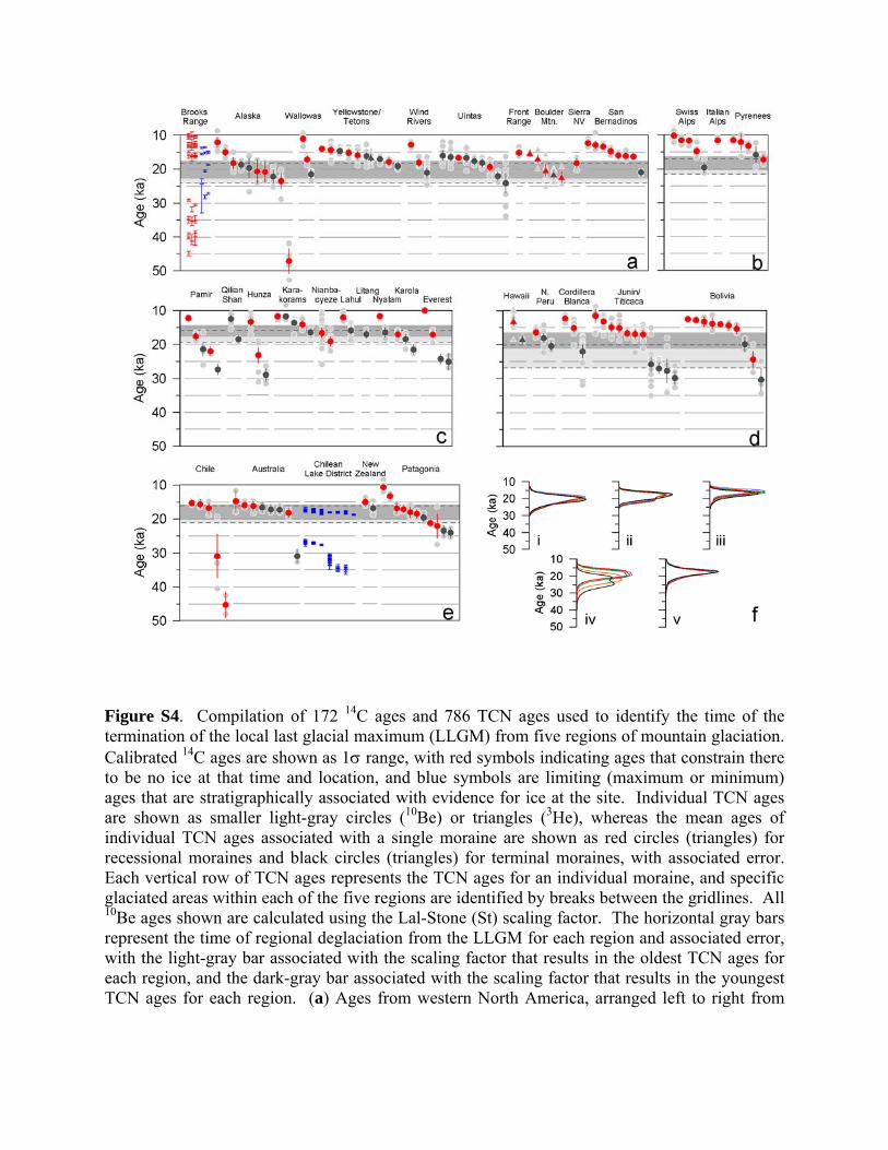
Figure S4. Compilation of 172 14C ages and 786 TCN ages used to identify the time of the termination of the local last glacial maximum (LLGM) from five regions of mountain glaciation. Calibrated 14C ages are shown as 1σ range, with red symbols indicating ages that constrain there to be no ice at that time and location, and blue symbols are limiting (maximum or minimum) ages that are stratigraphically associated with evidence for ice at the site. Individual TCN ages are shown as smaller light-gray circles (10Be) or triangles (3He), whereas the mean ages of individual TCN ages associated with a single moraine are shown as red circles (triangles) for recessional moraines and black circles (triangles) for terminal moraines, with associated error. Each vertical row of TCN ages represents the TCN ages for an individual moraine, and specific glaciated areas within each of the five regions are identified by breaks between the gridlines. All 10Be ages shown are calculated using the Lal-Stone (St) scaling factor. The horizontal gray bars represent the time of regional deglaciation from the LLGM for each region and associated error, with the light-gray bar associated with the scaling factor that results in the oldest TCN ages for each region, and the dark-gray bar associated with the scaling factor that results in the youngest TCN ages for each region. (a) Ages from western North America, arranged left to right from

north (Alaska) to south (California). (b) Ages from Europe. (c) Ages from Tibet. (d) Ages from the tropics and subtropics. (e) Ages from the Southern Hemisphere. (f) Probability distribution functions (pdfs) for the ages from each of the five regions that constrain the time of regional deglaciation, with five different pdfs for each region representing the five different scaling factors. (i) pdf for western North America, (ii) pdf for Europe, (iii) pdf for Tibet, (iv) pdf for tropics and subtropics, (v) pdf for Southern Hemisphere.

ICN standard assuming a 10Be half-life of 1.5 Myr (KNSTD3110). 3He ages were calculated using Lal (20) scaling and a sea-level, high-latitude production rate of 118 atoms/g⋅yr (21). Rock density for granitic lithologies was assumed to be 2.65 g/cm3, unless otherwise noted in the original publication. Erosion rates were set to zero for all samples. Snow cover corrections were made according to the suggestions of the original authors.

We identified outliers using a consistent, objective methodology. Obvious Holocene outliers were excluded (7 boulders on 3 moraines). Boulder ages >10 kyr from the other ages in a population were also excluded (10 boulders on 8 moraines). Thereafter, we used Chauvenet’s criterion to identify remaining outliers. This involves determining the probability of obtaining a date x standard deviations away from the mean of a population assuming a normal distribution. This probability was then multiplied by the number of samples in the population to determine how many dates one could expect to differ from the mean by this amount (x); dates returning values < 0.5 were deemed outliers. As Chauvenet’s criterion assumes normality, a Wilk-Shapiro test was performed first; only populations returning p-values >0.05 were considered to be normally distributed and subjected to Chauvenet’s criterion. We then calculated an unweighted mean moraine age, and assigned a 1σ error to this mean moraine age using the standard error of the boulder ages and a 6% production-rate uncertainty (22) added in quadrature.

Most of the dating of mountain-glacier fluctuations is based on TCN ages, which only constrain the timing of deglaciation, but there is additional information suggesting that in many places, mountain glaciers were near or at their maximum extent by ~30 ka. The two cases where 14C control exists, for example, suggest that glaciers in the Brooks Range, Alaska, were near their maximum extent by ~29 ka (Fig. S4a), and mid-latitude Chilean glaciers by ~35 ka (Fig. S4e). In addition, a number of TCN ages from moraines in Tibet and the tropics suggest fluctuations of ice margins at or near their maximum extent between 30 ka and the onset of regional deglaciation (Fig. S4). The onset of the last deglaciation for each of the five regions is defined here as occurring when all dated sites in a given region record ice retreat based on their 10Be chronologies. While any given moraine may predate this time, we consider this criterion to be a better representation of the timing of regional-scale deglaciation. To constrain this time interval, we slid a window forward through time until it intersected the mean age of a moraine at each site within its 1σ error bars. The window width was set to equal the average 2σ error on the terminal moraines in each region as ages within this window size presumably cannot be differentiated statistically. A cumulative distribution function (cdf) was computed from the ages of all moraines that intersect this window and the middle 68% of the cdf was used to define the 1σ age range of the onset of deglaciation. Ice Area-Volume Scaling and Sea-Level Change

The temporal correspondence of ice-sheet growth and sea-level lowering is supported by the spatial distribution of limiting ages constraining expansion of the LIS and SIS, the two largest Northern Hemisphere ice sheets which, with Antarctic ice, were the primary contributors to sea-level change (23). In the case of the LIS, the distribution of ages identifying ice-free areas before its LGM growth period (Fig. S2a-g) indicates that its size through much of MIS 3 up until ~32 ka was similar to its size during deglaciation 12-13 ka (24), which is between 56% and 63% of its LGM size (10). Between 32 and 26 ka, the LIS reached its maximum extent everywhere (Fig. 3b), thus representing a 37% to 44% increase in area over that of MIS 3.

We convert ice area (km2) to ice volume (km3) using the well-established relationship for an ice sheet on a hard bed (log[volume]=1.23[log[area]−1]) (25). Although this assumes that an ice sheet or ice cap is in equilibrium, this relationship was developed on ice sheets and ice caps in different mass balance states (both positive and negative) with single and multiple ice domes. These ice sheets and ice caps span four orders of magnitude in area (AIS to the Barnes Ice Cap) and climate conditions from temperate maritime (Iceland) to polar desert (Antarctica). The resulting error in the ice volume estimate is ~12%. This simple area-volume scaling relation suggests that the LGM volume of the LIS represented ~73 m of global sea level, in good agreement with results from ice-sheet models (26-28). Using the same scaling relation, the increase in LIS area between 33.0 and 26.5 ka represented 32 to 38 m of the ~50 m fall in global sea-level that occurred during this interval (i.e., from about -75 m to -125 m) (Fig. 3c). Similar time-distance constraints for the SIS suggest that it contributed a significant fraction of the remaining 12 to 18 m of sea-level fall to the LGM lowstand. In particular, the spatial distribution of ages from the SIS suggests that (1) much of the area covered by the LGM ice sheet was ice-free during MIS 3 (Fig. S2n-S2p), with ice likely being restricted to the central highlands along the Norwegian-Swedish border, and (2) that the ice sheet grew rapidly to its LGM size (14-20 m of sea level) (26, 29) between 29 and 27 ka. Integrated Summer Energy Huybers (30) defined the integrated summer energy as the sum of insolation intensity exceeding a threshold, where the threshold is the insolation value corresponding to a temperature of 0oC. Huybers recognized, however, that the threshold value will vary depending on such things as albedo, topography, and atmospheric greenhouse gas concentrations. We thus used a simulation of the LGM using a global climate model (31) to establish the relationship between insolation and temperature at sea level for LGM climate. We then used the elevations of the dated moraines used in this study from the five different regions (Fig. S5a) to lapse rate (6oC/1000 m) the insolation-temperature relationship values to those elevations (Fig. S5B), and used the corresponding time series of integrated summer energy for the associated threshold value at a given latitude (http://www.ncdc.noaa.gov/paleo/pubs/huybers2006b).

0 100 200 300 400Insolation (W m-2)

-40

-30

-20

-10

0

10

Tem

pera

ture

(o C) 60N

50N40N30N5S15S30S40S50S

80 60 40 20 0 -20 -40 -60Latitude (o)

0

1000

2000

3000

4000

5000A

ltitu

de (m

)a

b

Figure S5. (a) Elevations of LGM moraines deposited by mountain glaciers from western North America (black), Europe (blue), Tibet (orange), the tropics (red), Australia and New Zealand (brick red), and Patagonia (green). (b) Insolation-temperature relationship for different latitudes established by applying a lapse rate correction of 6oC 1000 m-1 to the LGM insolation-temperature relationship at sea level derived from a global climate model.

References

1. R. A. Kendall, J. X. Mitrovica, G. A. Milne, Geophysical Journal International 161, 679

(Jun, 2005). 2. S. E. Bassett, G. A. Milne, J. X. Mitrovica, P. U. Clark, Science 309, 925 (2005). 3. J. X. Mitrovica, W. R. Peltier, Journal of Geophysical Research 96, 20053 (1991). 4. J. X. Mitrovica, G. A. Milne, Quaternary Science Reviews 21, 2179 (2002). 5. M. Nakada, K. Lambeck, Geophysical Journal International 96, 497 (1989). 6. W. R. Peltier, Annual Review of Earth and Planetary Sciences 32, 111 (2004). 7. G. A. Milne, J. X. Mitrovica, Quaternary Science Reviews 27, 2292 (2008). 8. M. Stuiver, P. J. Reimer, Radiocarbon 35, 215 (1993). 9. R. G. Fairbanks et al., Quaternary Science Reviews 24, 1781 (2005). 10. A. S. Dyke, in Quaternary Glaciations - Extent and Chronology, Part II: North America,

J. Ehlers, P. L. Gibbard, Eds. (Elsevier Science and Technology Books, 2004), vol. 2b, pp. 373-424.

11. V. R. Rinterknecht et al., Science 311, 1449 (2006). 12. G. Balco, J. M. Schaefer, Quaternary Geochronology 1, 15 (Feb, 2006). 13. J. Clark et al., Geological Society of America Bulletin 121, 3 (2009). 14. G. Balco, J. O. Stone, N. A. Lifton, T. J. Dunai, Quaternary Geochronology 3, 174

(2008). 15. G. Balco, J. O. H. Stone, S. C. Porter, M. C. Caffee, Quaternary Science Reviews 21,

2127 (2002). 16. A. Mackintosh et al., Geology 35, 551 (2007). 17. D. C. Heroy, J. B. Anderson, Quaternary Science Reviews 26, (2007). 18. B. L. Hall, G. H. Denton, Geografiska Annaler 82A, 305 (2000). 19. G. Balco, J. Stone, N. Lifton, T. Dunai, Quaternary Geochronology, (2008). 20. D. Lal, Earth and Planetary Science Letters 104, 424 (1991). 21. J. M. Licciardi, M. D. Kurz, J. M. Curtice, Earth and Planetary Science Letters 246, 251

(2006). 22. J. O. Stone, Journal of Geophysical Research 105, 23 (2000). 23. P. U. Clark, A. C. Mix, Quaternary Science Reviews 21, 1 (2002). 24. A. S. Dyke et al., Quaternary Science Reviews 21, 9 (2002). 25. W. S. B. Paterson, The Physics of Glaciers: 3rd Edition. (Pergamon Press, New York,

1994), pp. 480. 26. G. H. Denton, T. J. Hughes, The Last Great Ice Sheets. (Wiley, New-York, 1981). 27. S. J. Marshall, T. S. James, G. K. C. Clarke, Quaternary Science Reviews 21, 175 (2002). 28. L. Tarasov, W. R. Pelteir, Quaternary Science Reviews 23, 359 (2004). 29. M. J. Siegert, J. A. Dowdeswell, M. Melles, qr 52, 273 (1999). 30. P. Huybers, Science 313, 508 (2006). 31. S. Hostetler, N. Pisias, A. Mix, Quaternary Science Reviews 25, 1168 (2006). 32. K. B. Cutler et al., Earth and Planetary Science Letters 206, 253 (2003). 33. R. L. Edwards et al., Science 260, 962 (1993). 34. J. Chappell, Quaternary Science Reviews 21, 1229 (2002). 35. E. Bard, B. Hamelin, R. G. Fairbanks, A. Zindler, n 345, 405 (1990).

36. W. R. Peltier, R. G. Fairbanks, Quaternary Science Reviews 25, 3322 (2006). 37. Y. Yokoyama, K. Lambeck, P. De Deckker, P. Johnston, L. K. Fifield, Nature 406, 713

(2000). 38. T. Hanebuth, K. Stattegger, P. M. Grootes, Science 288, 1033 (2000). 39. E. Bard et al., Nature 382, 241 (1996). 40. J. Ridge, in Geoarchaeology of Landscapes in the Glaciated Northeast, D. L. Cremeens,

J. P. Hart, Eds. (New York State Museum Bulletin, Albany, NY, 2003), vol. 497, pp. 15-45.