surface to surface intersections - mit - massachusetts...

Surface to Surface Intersections

N. M. Patrikalakis, T. Maekawa, K. H. Ko, H. Mukundan

May 2004

Slide No. Slide No. Slide No. Slide No. 2222

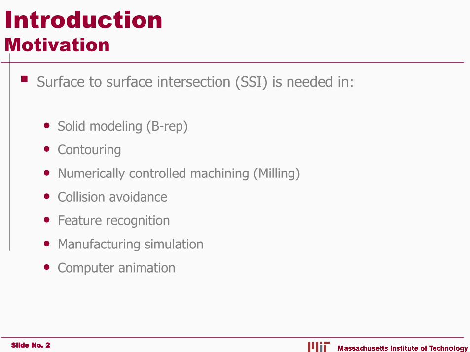
Introduction Motivation

Surface to surface intersection (SSI) is needed in:

• Solid modeling (B-rep)

• Contouring

• Numerically controlled machining (Milling)

• Collision avoidance

• Feature recognition

• Manufacturing simulation

• Computer animation


Introduction Background

Intersection of two parametric surfaces, defined in parametric spaces and can have multiple components [4].

An intersection curve segment is represented by a continuous trajectory in parametric space.

),(),( vut QP =σ1,0 ≤≤ vu1,0 ≤≤ tσ

10 σ 10 u0

1

t

0

1

v

Parametric space of ),( vuQ

Parametric space of ),( tσP3D Model Space

),( tσP

),( vuQ


IntroductionPossible Approaches

Three popular methods

• Lattice methods

Issues related to topology, missing roots.

• Subdivision based methods

Issues related to topology, extraneous roots.

• Marching scheme (Our Choice)

Intersection curve segment is computed through an IVP.


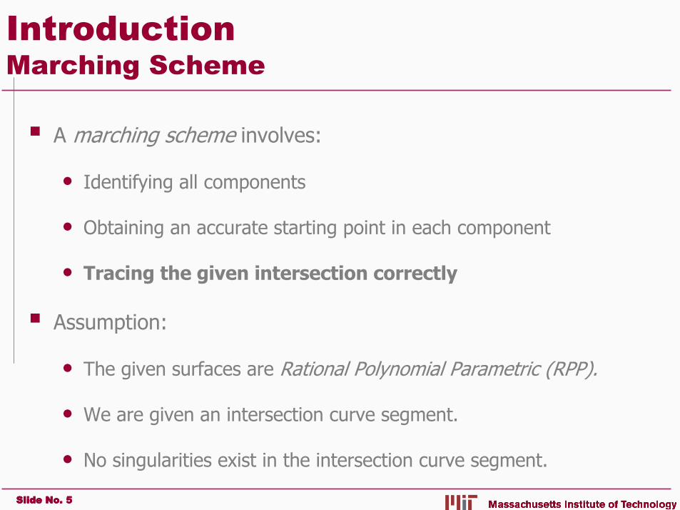
Introduction Marching Scheme

A marching scheme involves:

• Identifying all components

• Obtaining an accurate starting point in each component

• Tracing the given intersection correctly

Assumption:

• The given surfaces are Rational Polynomial Parametric (RPP).

• We are given an intersection curve segment.

• No singularities exist in the intersection curve segment.


IntroductionObjective

Given an error bound on the starting point in both parametric spaces, obtain a bound for the entire intersection curve segmentin 3D model space.

Strict Error Bound on Starting Point (Given) Strict Error Bound on the Entire Intersection Curve Segment (Goal)


Outline

Problem Formulation

Error Bounds in Parametric Space

Error Bounds in 3D Model Space

Results and Examples

Conclusions


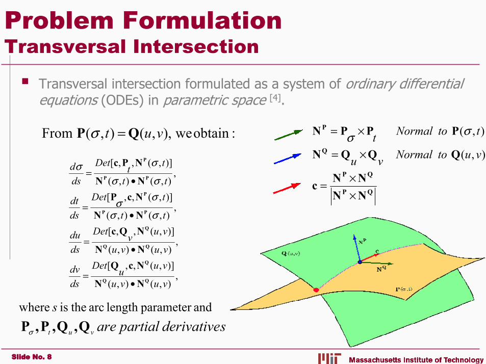
Problem FormulationTransversal Intersection

Transversal intersection formulated as a system of ordinary differential equations (ODEs) in parametric space [4].

,),(),(

)],(,,[

,),(),(

)],(,,[

,),(),(

)],(,,[

,),(),(

)],(,,[

vuvu

vuuDet

dsdv

vuvu

vuvDet

dsdu

tt

tDet

dsdt

tt

ttDet

dsd

QQ

Q

QQ

Q

PP

P

PP

P

NN

NcQNN

NQcNN

NcPNN

NPc

•=

•=

•=

•=

σσ

σσ

σσ

σσ

:obtainwe),,(),(From vut QP =σ

sderivativepartialarevut Q,Q,P,Pσ

andparameter length arc theis where s

QP

QP

Q

P

NNNNc

QQQN

PPPN

××=

×=

×=

),(

),(

vutoNormalvu

ttoNormalt σσ


Problem FormulationTangential Intersection

ODEs have the same form as in transversal intersection case

From the condition of equal normal curvatures we obtain the equation

where are functions of the first and second fundamental form coefficients of the surfaces.For a unique marching direction, and

• Thus if: or if:

surfaces. theof sderivative second theusing determined is

),(),(

,),(),(

)],(,,[',

),(),(

)],(,,[',

),(),(

)],(,,[',

),(),(

)],(,,['

c

QQQNPPPNNN

NcQ

NN

NQc

NN

NcP

NN

NPc

QP

QQ

Q

QQ

Q

PP

P

PP

P

vutoNormalvuandttoNormalt

vuvu

vuuDetv

vuvu

vuvDetu

tt

tDett

tt

ttDet

×=×=•

=•

=•

=•

=

σσ

σσ

σσσσ

σσ

0)'()')('(2)'( 22212

211 =++ tbtbb σσ

221211 ,, bbb

0)( 22112

12 =− bbb 0)( 222

211

212 ≠++ bbb

0,0 2211 ≠= bb,011 ≠b

11

12where,bb

t

t −=++= ν

νν

σ

σ

PPPPc

22

12,bbwhere

t

t −=++= µ

µµ

σ

σ

PPPPc


Problem FormulationVector IVP for ODE

Given a starting point (initial condition) belonging to an intersection curve segment, we can integrate the system of ODEs.

The system of ODEs with the starting point represents an initial value problem (IVP).• Written in vector notation as:

0)(),( y0yyfy ==dsd

=

),,,(

),,,(

),,,(

),,,(

4

3

2

1

vutf

vutf

vutf

vutf

dsdvdsdudsdtdsd

σ

σ

σ

σσ


Outline

Problem Formulation

Error Bounds in Parametric Space• Review of Standard Schemes

• Interval Arithmetic

• Validated Interval Scheme



Conclusions


Error Bounds in Parametric SpaceError Bounds in Parametric SpaceError Bounds in Parametric SpaceError Bounds in Parametric SpaceReview of Standard Schemes

Well-known Standard Schemes:• Runge-Kutta Method• Adams-Bashforth Method• Taylor Series Method

Properties of Standard Schemes:• They are approximation schemes and introduce a truncation error• They do not consider uncertainty in initial conditions• They are prone to rounding errors• They suffer from straying or looping near closely spaced features


Error Bounds in Parametric SpaceError Bounds in Parametric SpaceError Bounds in Parametric SpaceError Bounds in Parametric SpaceInterval Arithmetic (Introduction)

Intervals are defined by [2]:

Example:

Basic interval arithmetic operations are defined by:

[ ] ][3.142 , 3.1414635897932383.14159265

πππ

=∈= K


Error Bounds in Parametric SpaceError Bounds in Parametric SpaceError Bounds in Parametric SpaceError Bounds in Parametric SpaceInterval Arithmetic (Solution of IVPs)

For strict bounds for IVPs in parametric space, we employ a validated interval scheme for ODEs [3].

The error in starting point is bounded by an initial interval.

Interval solution represents a family of solutions passing through the initial interval satisfying the governing ODEs.


Error Bounds in Parametric SpaceError Bounds in Parametric SpaceError Bounds in Parametric SpaceError Bounds in Parametric SpaceValidated Interval Scheme (Introduction)

Every step of a validated interval scheme involves [3]:

• Computing an interval valued function such that:

and

The width of the is below a given tolerance

• Verifying the existence and uniqueness of the solution in

,)]([)( ss yy ∈ ],[ 1+∈∀

jj sss

1[ , ].+j js s

)]([ sy

)]([ sy


Error Bounds in Parametric SpaceError Bounds in Parametric SpaceError Bounds in Parametric SpaceError Bounds in Parametric SpaceValidated Interval Scheme (Overview)

One step of a validated interval scheme is done in two phases:

• Phase I Algorithm

A step size

An a priori enclosure such that:

• Phase II Algorithm

Using compute a tighter boundat .

]~[ jy

]~[ jy ][ 1+jy

],[],~[)( 1+∈∀∈ jjj sssysy

jjj ssh −= +1

Phase 1:

1+js


Error Bounds in Parametric SpaceError Bounds in Parametric SpaceError Bounds in Parametric SpaceError Bounds in Parametric SpaceValidated Interval Scheme (Phase I : Validation)

A pair of and satisfying the relation:

• This assures existence and uniqueness of the solution.• This method is called a constant enclosure method [3].

The a priori enclosure bounds the true solution in the parametric space .

Numerical implementation• Choosing a and,

• Iterating to find a corresponding .

jjjj h])~([][]~[ yfyy +⊇

jh]~[ jy

jh]~[ jy

]~[ jy],[ 1+∈∀ jj sss


Error Bounds in Parametric SpaceError Bounds in Parametric SpaceError Bounds in Parametric SpaceError Bounds in Parametric SpaceValidated Interval Scheme (Phase II : Tighter Bound)

Using the a priori enclosure we• find a tighter bound at [3].

This phase helps in the propagation of the solution by providingan initial interval for the successive step.

The key idea is to use:• Interval version of Taylor’s formula [3].

1+js

1[ ][ ]

11

[ ] [ ] ([ ]) ([ ])k

i k kij j j j j j

ih h

−

+=

= + +∑y y f y f yy y f y f yy y f y f yy y f y f y%

][ 1+jy

[ ]

[3]

where ([ ]) represents the

obtained using a techniquecalled Automatic Differentiation .

i thj i Taylor coefficientf yf yf yf y


Error Bounds in Parametric SpaceError Bounds in Parametric SpaceError Bounds in Parametric SpaceError Bounds in Parametric SpaceValidated Interval Scheme (Application to SSI)

We represent the surfaces as interval surfaces.• Interval surfaces have interval coefficients and are written as:

We obtain a vector interval ODE system :

With an interval initial condition :

)])(([ sdsd

dsdv

dsdu

dsdt

dsd T

yfy ==

σ

[ ] [ ] ),(and),( vut QP σ

[ ]Tvut ][][][][][ 00000 σ=y


Error Bounds in Parametric SpaceError Bounds in Parametric SpaceError Bounds in Parametric SpaceError Bounds in Parametric SpaceValidated ODE solver produces a priori enclosures in parametric space of each surface, guaranteed to contain the true intersection curve segment.

The union of a priori enclosures bounds the true intersection curve segment in parametric space.


Outline

Problem Formulation




Conclusions


Error Bounds in 3D Model SpaceError Bounds in 3D Model SpaceError Bounds in 3D Model SpaceError Bounds in 3D Model SpaceMapping into 3D Model Space

Mapping from parametric space to 3D model space• using corresponding surfaces• coupled with rounded interval arithmetic evaluation

Ensures continuous error bounds in 3D model space [1]

guaranteed to contain the true curve of intersection.

[ ] [ ] ),(o),( vurt QP σ


Outline

Problem Formulation




Conclusions


Torus and cylinder Two bi-cubic surfaces

Results & Examples Error Bounds in 3D Model Space (Transversal)

0.02 0.001

Self intersection of a bi-cubic surface


Tangential intersections of parametric surfaces

Results & Examples Error Bounds in 3D Model Space (Tangential)


Validated ODE solver can correctly trace the intersection curve segment even through closely spaced features, where standard methods fail.

Results & Examples Preventing Straying and Looping

Adams-Bashforth Runge-Kutta

Result from a validated interval

scheme

Perturbation Steps Required bythe Method

+0.000003 1139

0.0 Singularity Reported

-0.000003 1303

σ

σ

σ

t

t

t


Outline

Problem Formulation




Conclusions


ConclusionsMerits

We realize validated error bounds in 3D model space which enclose the true curve of intersection.

The scheme can prevent the phenomenon of straying or looping.

The scheme can accommodate the errors in:• initial condition

• rounding during digital computation

Validated error bounds for surface intersection is essential in interval boundary representation for consistent solid models [5].


ConclusionsLimitations and Future Work

Limitations• We assume that we have

Identified each intersection curve segmentStrict error bound on the starting point

• Increasing width of the interval solutions due toRoundingPhenomenon of wrapping

Scope for future work• Identification of all components• Accurate evaluation of starting points in each of the component


Acknowledgements

• National Science Foundation

• Prof. T. Sakkalis

• Prof. N. Nedialkov


References 1. Tracing surface intersections with a validated ODE system solver, Mukundan, H., Ko, K.

H., Maekawa, T. Sakkalis, T., and Patrikalakis, N. M., Proceedings of the Ninth EG/ACM Symposium on Solid Modeling and Applications, G. Elber and G. Taubin, editors. Genova, Italy, June 2004. Eurographics Press.

2. Moore R. E.. Interval Analysis. Prentice-Hall, Englewood Cliffs, 1966.

3. Nedialkov N. S.. Computing the Rigorous Bounds on the Solution of an Initial Value Problem for an Ordinary Differential Equation. PhD thesis, University of Toronto, Toronto, Canada, 1999.

4. Patrikalakis N. M. and Maekawa T.. Shape Interrogation for Computer Aided Design and Manufacturing. Springer-Verlag, Heidelberg, 2002.

5. Sakkalis T., Shen G. and Patrikalakis N.M., Topological and Geometric Properties of Interval Solid Models, Graphical Models, 2001.

6. Grandine T. A., Klein F. W.: A new approach to the surface intersection problem. Computer Aided Geometric Design 14, 2 (1997), 111–134. 650.

surface to surface intersections - mit - massachusetts...

Documents