surprise! you are accepted to college: an analysis of idaho’s
TRANSCRIPT

SURPRISE! YOU ARE ACCEPTED TO COLLEGE: AN ANALYSIS OF IDAHO’S
DIRECT ADMISSIONS INITIATIVE
by
Carson Howell
A dissertation
submitted in partial fulfillment
of the requirements for the degree of
Doctor of Philosophy in Public Policy and Administration
Boise State University
December 2018

© 2018
Carson Howell
ALL RIGHTS RESERVED

BOISE STATE UNIVERSITY GRADUATE COLLEGE
DEFENSE COMMITTEE AND FINAL READING APPROVALS
of the dissertation submitted by
Carson Howell
Dissertation Title: Surprise! You are Accepted to College: An Analysis of Idaho’s
Direct Admissions Initiative
Date of Final Oral Examination: 12 October 2018
The following individuals read and discussed the thesis submitted by student Carson
Howell, and they evaluated his presentation and response to questions during the final oral
examination. They found that the student passed the final oral examination.
Stephanie L. Witt, Ph.D. Chair, Supervisory Committee
Gregory Hill, Ph.D. Member, Supervisory Committee
Stephen M. Utych, Ph.D. Member, Supervisory Committee
The final reading approval of the dissertation was granted by Stephanie L. Witt, Ph.D.,
Chair of the Supervisory Committee. The dissertation was approved by the Graduate
College.

iv
DEDICATION
For my beautiful and wonderful wife, Michelle. You really are the best. For my
children—Daegan, Sierra, Maddox, Kyler, and Shayla. The greatest honor I could ever
receive was to be your dad.

v
ACKNOWLEDGEMENTS
This dissertation represents the culmination of efforts of many individuals and
two different universities. I have been fortunate to have the support of many mentors and
caring individuals throughout this journey.
I would like to first thank Dr. Stephanie Witt. Our friendship goes back long
before we were connected academically. She encouraged me to pursue a career in public
service and I am grateful for her support. She was my advocate as I transferred to Boise
State University in the middle of a doctoral program. Through her mentorship and
guidance, I finally arrived at this point.
Dr. Nick Hillman was a big part of why I started this journey through the
Education Leadership and Policy program at the University of Utah. He has been a
sounding board through my many iterations of dissertation ideas and the annual pep talk.
Thank you Nick for your continued friendship and mentoring.
I would also like to acknowledge my friend, Dr. Jean Henscheid for all of her
support. Her time spent helping me and reviewing draft after draft of this dissertation has
been critical in this accomplishment. Thank you, Jean.
I would also like to thank Matt Freeman, the Executive Director at the Idaho State
Board of Education. Thank you for fostering an environment where innovation can be
combined with bureaucracy. That is a difficult task to accomplish in state government
and I appreciate the willingness to entertain more than one crazy idea. While there are
structural differences that might have limited the creation of the Direct Admissions

vi
program in other states, I am convinced that cultural differences may have been an even
bigger obstacle in other systems. Thank you for being a visionary.
I must also acknowledge the staff at the Office of the State Board of Education
who have supported me. Blake Youde was a valuable partner in our efforts within the
Office of the State Board of Education to make radical changes that could improve the
life of students in Idaho. Direct Admissions would not have happened without his
partnership. Tracie Bent has encouraged me along the path and I appreciate her constant
urging and support through this process. Tracie helped keep our ideas grounded in the
realm of possibility.
Lastly, I would like to thank my family for their support. My mom and dad
instilled in me a desire to go to college. I never imagined that I would go to this level of
education, but they have been supportive all along the way. Thank you mom for your
support. Dad, I would have loved for you to be around to see this.
Most importantly, I owe my wife, Michelle, a large debt of gratitude. Many
“family” activities were planned without my attendance so that I could stay home and
work on writing. Michelle, you have been nothing but supportive through this entire
process. I love you and owe you tremendously.

vii
ABSTRACT
In an effort to improve the rate at which Idahoans ‘go on’ to postsecondary
education, Idaho launched an initiative called Direct Admissions in the fall of 2015. This
initiative informed students and their parents that the student had already been accepted
to at least six of Idaho’s public colleges and universities, even before the student had
applied. Although the students still needed to apply, the letters guaranteed the student a
seat at any of the colleges listed in their Direct Admissions letter. The goal of the
initiative was to encourage students to enroll in one of Idaho’s public colleges or
universities through reducing the barriers to entry. It was designed to specifically
encourage those students who had not yet decided on whether they would attend college.
Idaho’s Direct Admissions process succeeded in positively influencing the enrollment
and application behavior of those students who were identified as the target populations
for the process.
As this dissertation is looking at student behavior, a framework of behavioral
economics, specifically Prospect Theory and the Endowment Effect, is employed to
guide the understanding of the outcomes of Direct Admissions. While the analysis
specifically focuses on the Direct Admissions initiative, this dissertation provides a guide
for broader application of behavioral economics as a framework for public administration
research. Because the design of Direct Admissions adhered to the tenants of both
Prospect Theory and the Endowment Effect, the process worked for the targeted students.

viii
A mixed methods approach is used by looking at the student-level application and
enrollment data for students participating in the program as well as survey responses
from students who received the letter. A series of regressions are used to evaluate how
the Direct Admissions letters are correlated with a change in college enrollment behavior.
A survey of Idaho students who received a Direct Admissions was also used to measure
the influence the Direct Admissions letters had in the college application behavior of the
students.

ix
TABLE OF CONTENTS
DEDICATION ............................................................................................................... iv
ACKNOWLEDGEMENTS ............................................................................................. v
ABSTRACT ..................................................................................................................vii
LIST OF TABLES ........................................................................................................xii
LIST OF FIGURES ...................................................................................................... xiv
CHAPTER ONE: INTRODUCTION .............................................................................. 1
Background .......................................................................................................... 2
Idaho’s Rationale ................................................................................................. 5
Who are Idaho’s Students? ................................................................................... 9
Direct Admissions Launched.............................................................................. 11
Purpose of Study ................................................................................................ 12
Outline ............................................................................................................... 14
CHAPTER TWO: THEORIES OF BEHAVIOR ........................................................... 17
Theories of Behavior .......................................................................................... 18
Utility Theory ......................................................................................... 18
Behavioral Economics ............................................................................ 19
Behavioral Economics and Early Links to Public Administration ....................... 20
Prospect Theory...................................................................................... 21
The Endowment Effect ........................................................................... 24

x
Explaining Citizen Behavior .............................................................................. 26
Behavioral Economics of Students ..................................................................... 27
The Role of Value .................................................................................. 28
Direct Admissions and Prospect Theory ................................................. 29
Direct Admissions and The Endowment Effect ....................................... 30
CHAPTER THREE: METHODOLOGY ....................................................................... 32
Research Design and Methods............................................................................ 32
Data Sources ...................................................................................................... 32
Methods – Quantitative ...................................................................................... 36
Linear Probability Model Regression on College Enrollment .................. 38
Methods – Survey of Students ............................................................................ 41
Limitations of Study........................................................................................... 43
CHAPTER FOUR: QUANTITATIVE RESULTS ......................................................... 46
Enrollment Trends ............................................................................................. 46
Variables ............................................................................................................ 49
General Statistics of Variables............................................................................ 49
Linear Probability Model ................................................................................... 55
CHAPTER FIVE: SURVEY RESULTS ........................................................................ 62
Results ............................................................................................................... 62
Students Who Indicated “No Impact” from Direct Admissions ............... 67
Students Who Indicated “Negative Impact” from Direct Admissions ...... 67
Students Who Indicated “Positive Impact” from Direct Admissions ....... 68
Impact and Additional Factors ................................................................ 70

xi
CHAPTER SIX: DISCUSSION..................................................................................... 75
Discussion.......................................................................................................... 75
Implications for Practice .................................................................................... 77
Direct Admissions and Behavioral Economics ................................................... 78
Behavioral Economics as a Public Administration Theory.................................. 83
Areas of Future Research ................................................................................... 84
Conclusion ......................................................................................................... 86
REFERENCES .............................................................................................................. 87
APPENDIX A ............................................................................................................... 94
Additional Information ....................................................................................... 95

xii
LIST OF TABLES
Table 1.1 Direct Admissions Letters ........................................................................3
Table 1.2 Definitions of Terms .................................................................................5
Table 1.3 Percent of High School Graduates Going Directly to College - 2010 ........5
Table 1.4 Go-On Percentages and Other State Characteristics ................................ 10
Table 2.1 Prospect Theory Scenario I ..................................................................... 22
Table 2.2 Prospect Theory Scenario II .................................................................... 23
Table 2.3 Endowment Effect Experiment ............................................................... 26
Table 3.1 Percent of Church of Jesus Christ of Latter-day Saints Adherents by
County, 2010 (Highest to Lowest) .......................................................... 34
Table 3.2 Variables, Variable Level, and Variable Types ....................................... 36
Table 4.1 Fall Immediate Enrollment Trends at Idaho Public Colleges, Academic
Years of High School Graduates 2012-2013 through 2015-2016 ............. 46
Table 4.2 T-test of Significance of Enrollment for Academic Years 2014-15 and
2015-16 .................................................................................................. 48
Table 4.3 Summary of Variables, Student Enrollment Fall 2016 ............................ 49
Table 4.4 Crosstabs of Free or Reduced-Price Lunch and Direct Admissions ......... 51
Table 4.5 Significance Levels of Relationships Between Type of Direct Admissions
Letter Received and Student Characteristics ........................................... 51
Table 4.6 Percentage of Enrolled Students by Characteristic .................................. 55
Table 4.7 Regression of Enrollment and Selected Variables with Interaction
Variables ................................................................................................ 57

xiii
Table 5.1 How Much of an Impact Did Your Direct Admissions Letter Have in Your
Deciding to Attend College After High School? ..................................... 63
Table 5.2 How Much of an Impact Did Your Direct Admissions Letter Have in Your
Deciding to Apply to a Particular College? ............................................. 63
Table 5.3 Most Important Factors for Selecting a Particular College ...................... 65
Table 5.4 Survey Responses on Level of Impact of Direct Admissions................... 66
Table 5.5 Direct Admissions Impact by Parental Education Level .......................... 70
Table 5.6 Survey Responses on Communication with Parents ................................ 72
Table 5.7 Survey Responses on Communication with Counselor or Teacher .......... 73
Table 6.1 Correlation of Direct Admissions Letter and Student Characteristics ...... 76
Table 6.2 Student Self-Reported Positive Impact of Direct Admissions on
Application Behavior by Subgroup ......................................................... 77
Table A.1 Survey Instrument .................................................................................. 95
Table A.2 Go-On Percentages and Other State Characteristics ................................ 98

xiv
LIST OF FIGURES
Figure 1.1 Percent of High School Graduates Going Directly to College - 2010 ........7
Figure 2.1 Value Function (Kahneman & Tversky, 1979) ........................................ 24

1
CHAPTER ONE: INTRODUCTION
The Idaho State Board of Education (SBOE) unanimously approved Direct
Admissions in August 2015. This new program was designed to make it easier for
students to enroll in college directly from high school. This analysis asks, did it work?
The research reported here employed quantitative methods to run a series of regressions
on application and enrollment data collected by the SBOE and qualitative analysis on
data from an SBOE survey of students who had participated in Direct Admissions.
Recognizing that enrollment behavior can differ between subgroups, the quantitative
analysis examined behavior among subgroups by gender, socioeconomic status, and
race/ethnicity.
The qualitative analysis of survey data examined whether this initiative influenced
student attitudes about postsecondary education. To conduct the survey, the SBOE
collected names of students who had applied to one of the eight Idaho public institutions
of higher education. Those students who had applied prior to the stated deadline of
February 15, 2016 through Direct Admissions received a survey. Responses from
students are coded for the influence Direct Admissions had on their attitudes toward
postsecondary education. Direct Admissions was designed to make it easier for all
students to enroll in education past high school. I use this study to explore a theoretical
model that may explain how policies influence the behavior of a targeted audience. The
theoretical framework of behavioral economics, specifically Prospect Theory and the
Endowment Effect is used to help explain student behaviors and attitudes. Results of this

2
inquiry suggest that Direct Admissions was successful in encouraging college enrollment
and in improving student attitudes toward postsecondary education. However, the
influence of Direct Admissions was felt more greatly among students who were least
likely to consider attending college prior to receiving a Direct Admissions letter.
This study also looks at how the framework of behavioral economics may prove
useful for future policy studies in both higher education and public administration in
general.
Background
The SBOE acts as both the Board of Regents for the public baccalaureate granting
colleges and universities as well as the governing and policy board for K-12 public
education. This is different than many states where there is a separate governing board
for K-12 public education and another board for higher education. The Idaho Constitution
Article IX, § 2 states, “the general supervision of the state educational institutions and
public school system of the state of Idaho, shall be vested in a state board of education.”
Increasing college enrollment is an effort of each state higher education governing
body. These efforts include providing scholarships, offers of free college, and guaranteed
admission programs (Cornwell, Mustard, & Sridhar, 2006; Farrell & Kienzl, 2009;
Heller, 1999; Horn, Flores, & Orfield, 2003; Long, Saenz, & Tienda, 2010; Niu &
Tienda, 2010; Perna, Rowan-Kenyon, Bell, Thomas, & Li, 2008; Pingel, Parker, &
Sisneros, 2016; Taylor & Lepper, 2018). These policies are designed to encourage more
students to enroll in college.
At the Board’s August 2015 meeting, the eight members of the Board
unanimously approved Direct Admissions. This program proactively admits every

3
graduating high school senior into college without the student applying. The student and
their parents are sent a letter informing them of the Idaho public institutions to which the
student has already been accepted. Parents were engaged in the process because of the
correlation between parental involvement and college enrollment behavior (Perna &
Titus, 2005; Rowan-Kenyon, Bell, & Perna, 2008).
Each student receives one of two letters based on the student’s GPA and
SAT/ACT score: A “Group of 6” or a “Group of 8” letter. The institutions included in
each of these letters are listed in Table 1.1. Students who meet the “Group of 8”
benchmark are admitted to all eight public institutions, including Boise State University,
the University of Idaho, and the academic programs at Idaho State University. These
universities represent the more selective institutions in Idaho. The remaining students are
not admitted to Boise State University or the University of Idaho and are only admitted to
the technical programs at Idaho State University. The hope is that informing students that
they have already been accepted, the barriers to entry will be reduced and the student
would be more likely to enroll in college.
Table 1.1 Direct Admissions Letters
Group of 6 Group of 8
College of Southern Idaho College of Southern Idaho
College of Western Idaho College of Western Idaho
Eastern Idaho Technical College Eastern Idaho Technical College
Idaho State University - College of
Technology1 Idaho State University
Lewis-Clark State College Lewis-Clark State College
North Idaho College North Idaho College
Boise State University
University of Idaho
1 Idaho State University – College of Technology delivers the career and technical education
programs at the university. These programs include certificate programs of varying lengths, an Associate of
Applied Science degree and a Bachelor of Applied Science degree.

4
Included in the Direct Admission program, any application fee students pay when
they complete their application form is counted toward their first tuition bill in the fall
semester. For example, if a student were to be admitted to and select the University of
Idaho, the $60 application fee would then be used as a deposit, which the student would
see as a credit on the fall tuition bill.
The Board designed the program in the hopes that by eliminating the ambiguity of
the postsecondary selection process and by “eliminating” the application fee, the process
for a student to enroll in college is simplified to the point that more students choose to
attend college. Idaho’s plan is different than other guaranteed enrollment plans in other
states.
Idaho’s plan eliminates the competition between students seen in states with
guaranteed percentage plans (Ehrenberg, 2004; Kain, O’Brien, & Jargowsky 2005). The
Board’s stated goal is that every student will have access to postsecondary education. In
order to let the student know that she has access to a public postsecondary institution,
each graduating student receives a Direct Admissions letter. The only barrier to receiving
the letter for all eight institutions is the student’s own performance, based on the
student’s college entrance exam score and the student’s GPA. While not likely, it is
entirely possible that every senior receives a group of eight letter. The Idaho policy
guarantees admission to every student. Because of the differences in Idaho’s program
compared to programs in other states, this analysis adds to the body of research of college
enrollment initiatives and their effectiveness.
The purpose of the study reported here was to examine whether the policy
increased the number of students enrolling in an Idaho public college. In order to best

5
understand the analysis, I present a definition for terms the reader will encounter in this
study. These are presented not only to help the reader better understand the study, but
also allows those interested in replicating the study a framework upon which to build.
The terms and definitions are presented in Table 1.2.
Table 1.2 Definitions of Terms
Term Definition
Enrollment
Measured by attendance in an Idaho public college or university
on the tenth day of the fall semester immediately after high
school graduation
College Broad term including all postsecondary institutions
Behavior
Empirical phenomenon of any observable overt act or steps taken
by an individual prior to acting
Go-on Rate
The rate at which students enroll in college in the fall semester
immediately after high school graduation
Idaho’s Rationale
Prior to the adoption of Direct Admissions, Idaho was recognized for its low go-
on rate. Idaho’s go-on rate was the lowest in the country at 45.1% in 2010 as reported by
the National Center for Higher Education Management Systems (see Table 1.3 and
Figure 1.1). The fall 2010 immediate-from-high-school go-on rate was more than 17
percentage points lower than the national average.
Table 1.3 Percent of High School Graduates Going Directly to College - 2010
State %
Mississippi 78.8
Connecticut 78.7
Massachusetts 73.2
New Mexico 72.4
South Dakota 71.8
Minnesota 70.9
Nebraska 69.5
New York 68.9
New Jersey 68.6
South Carolina 68.3
Georgia 67.7

6
North Dakota 67.4
Iowa 66.6
Indiana 65.8
Arkansas 65.4
Rhode Island 65.4
Kansas 64.7
Louisiana 64.7
New Hampshire 64.3
Maryland 64.1
North Carolina 64.1
Virginia 63.8
Hawaii 63.6
Alabama 63.2
Florida 63.1
Kentucky 62.9
Nation (Avg.) 62.5
Tennessee 62.1
Michigan 61.9
California 61.7
Ohio 61.5
Missouri 61.4
Colorado 61.2
Pennsylvania 60.9
Montana 60.5
Wyoming 60.4
Oklahoma 60.2
Wisconsin 60.1
West Virginia 59.2
Illinois 58.7
Arizona 57.9
Maine 56.2
Texas 56.2
Vermont 53.5
Utah 53.3
Nevada 51.8
Washington 48.3
Oregon 47.8
Delaware 47.3
Alaska 46.4
Idaho 45.1

7
Figure 1.1 Percent of High School Graduates Going Directly to College - 2010

8
At the same time the go-on rate data were reported, the Center on Education and
the Workforce based at Georgetown University released a report (Carnevale, Smith, &
Strohl, 2010). This report, titled “Help Wanted: Projections of Jobs and Education
Requirements Through 2018,” was quickly recognized around the country as evidence
that states needed to focus on college attendance rates. In the report, Georgetown
researchers completed a state-by-state breakdown of the economy and what level of
education was needed to fill the projected workforce needs. The report stated that without
a substantial growth in the number of residents with a postsecondary degree or certificate,
the state’s economy would suffer and would lose good jobs to those states that could
provide the educated workforce needed (Carnevale, Smith, & Strohl, 2010).
The low go-on rate that threatened to undermine Idaho’s economy entered public
debate in the mid-2000s through a series of television, radio, newspaper and online ads
released by J.A. and Kathryn Albertson Family Foundation. The ads referenced the 2010
data from the National Center for Higher Education Management Systems (NCHEMS) as
previously shown in Table 1.3 and connected the problem of educational attainment to
low go-on rates. If high school graduates did not go on to college, those individuals
would never complete college. If individuals did not complete college, the state would
suffer.
The adverse effects of a low go-on rate also impacts the individual. A report from
Economic Modeling Specialists International states that there is a 9:1 return on
investment by earning an Idaho bachelor’s degree (2015). Skills learned through a
college education allow individuals to be more productive which results in higher wages
(Obradovic, 2009; London, 2006). Over time, education is shown to play a vital role in

9
the increase to wages, especially when considering the degree a student earns (Lemieux,
2006; Walters, 2004). Not only are salaries generally higher for college-educated
individuals, but the ability for those graduates to find a job is also increased.
The Federal Reserve Bank of San Francisco (2014) has noted that, “A college
degree comes with higher earnings, some insurance from the ups and downs in the
economy, and a path up the economic ladder” (p. 8). A study by the Bureau of Labor
Statistics showed that as of November 2015, an adult with less than a high school
education had a national unemployment rate of 6.9 percent. An adult with a bachelor’s
degree or higher had a national unemployment rate of only 2.5 percent (Bureau of Labor
Statistics, November 2015). As education level increases, the rate of unemployment
decreases. For Idaho’s economy and for its citizens, it was clear that the state needed to
increase the number of students attended college.
Who are Idaho’s Students?
Idaho knows that students do not go on to college at the same rates as other states.
As previously mentioned, in 2010, Idaho ranked at the bottom of the go-on percentage
among all states. Go-on rates were not the only area where Idaho differed from the rest of
the states (see Table 1.4). These data were collected from the U.S. Census Bureau, the
National Center for Higher Education Statistics, and the U.S. Religion Census. The full
list of states can be found in Table A.2 in Appendix A.

10
Table 1.4 Go-On Percentages and Other State Characteristics
State Go-On
%
% in
Poverty
%
Male
%
Hispanic
%
Urban
%
LDS
Average
of States
62.2 9.5 49.3 10.1 73.6 3.5
Idaho 45.1 9.7 50.1 10.6 70.6 26.1
College enrollment has been shown to correlate with many factors. Research has
shown that factors such as socioeconomic status, race, ethnicity, gender, and urbanicity
all are correlated with student enrollment behavior (Adelman, 2002; Averett & Burton,
1996; Black & Sufi, 2002; Cabrera & La Nasa, 2000; Goldin, Katz & Kuziemko, 2006;
Gose, 1999; Hurtado, Inkelas, Briggs, & Rhee, 1997; Light & Strayer, 2002; McFarland,
J. et al., 2018; Wagner & Blackorby, 1996; Thomas, 1980). College attending behaviors
varied between subgroups. For example, higher income students enroll at higher rates
than lower income students, females enroll at higher rates than males, and white students
enroll at higher rates than Hispanic students. As a state with high relative poverty rates,
more males than females, and a high rural population, it is no surprise that Idaho ranks at
the bottom in college attendance rates.
Any factor that could result in a student deferring college attendance is a concern
as delaying enrollment has shown to have a significant effect on college attendance at all
(Perez-Arce, 2015). Delayed enrollment is more of a factor in Idaho than in most other
states given the high number of young men who choose to serve a mission directly from
high school for the Church of Jesus Christ of Latter-day Saints. As noted in Table 1.4
26.1 percent of Idaho’s population identifies as adherents to the Church of Jesus Christ of
Latter-day Saints (LDS), or Mormon (U.S. Religion Census, 2010). In 2012, the

11
President of the LDS Church announced that men would be eligible for missionary
service at the age of 18, a change from what had previously been 19.2 According to the
LDS faith, missionary service is a calling from God and is strongly recommended for all
men, who serve as full-time missionaries for 24 months. During that time, the vast
majority of missionaries will move away from home and are precluded from taking any
college courses. The impact of this age change and the emphasis on missionary service
results in lower college attendance rates for LDS adherents immediately after graduating
high school.
Direct Admissions Launched
In late 2014, Chuck Staben, President of the University of Idaho, approached the
other public college and university presidents with a challenge to make it easier for
students to enroll at their institutions. Staben described how he had gone through the
University of Idaho’s admission process as if he were a student and found it cumbersome.
He posited that the amount of data automatically collected on students should allow the
state to directly admit high school graduates into Idaho’s colleges. From that suggestion,
SBOE staff developed Direct Admissions and launched the program in the fall of 2015.
The belief of Staben and Board staff was that making the processes of application
and admission easier would result in more students going on to college. The hope was
that students who had not thought that they could go on to college, or were on the fence
about their decision to go on to college, would respond to positive messaging about the
2 The age for women to serve a religious mission changed at the same time from 21 to 19. Since
that timing would allow for most women to attend college for approximately one year prior to leaving on a
mission, the impact of the change in eligible mission ages is more likely to affect the enrollment behavior
of men.

12
student’s acceptance to college. The Board believed that by informing students that they
had been accepted even before applying, more students would in turn apply and enroll in
college since the question of the student’s qualifications and eligibility had already been
addressed.
Staben’s hunch and the hopes of the Board are borne out in the literature.
Research indicates that lower socioeconomic students are more responsive to changes in
admissions policy and that changing the admissions policy to accept all students may
result in as much as a 3.8 percent increase in college attendance (Bishop, 1977). Bishop
found that the populations least likely to go-on are those most affected by changes in
admission policy and stated that with changes in the admission policy, the proportion
entering from the bottom-ability quartile would rise by 6.7 percent (p. 299). Given the
demographics of the students in Idaho, Bishop’s estimates could result in significant and
visible increases in college enrollment in Idaho.
Purpose of Study
This study explores whether Direct Admissions is positively correlated with
student enrollment directly after high school. The Idaho Direct Admissions plan was
developed to reduce the barriers that students face in attending college. An evaluation of
this policy then needs to ask a single question – is it working? Therefore, my research
questions are focused on if and how Direct Admissions works.
My first question is “does Idaho’s Direct Admission initiative predict higher rates
of postsecondary attendance?” My second question is “how much influence does the
Direct Admissions initiative have on a student’s college application behavior?”

13
The intended goal of Direct Admissions is for students to attend college at an
Idaho public institution. I chose to evaluate the program to see if the program positively
correlates with college enrollment behavior of a student. I recognize that there are many
factors that could influence a student’s college enrollment behavior, such as financial aid,
health, or any number of life events. This study is an evaluation of the Direct Admissions
program and not a broader study on the many reasons why students do not attend college.
The first question could be answered through a quantitative analysis. By looking
at the different subpopulations and their enrollment behavior, I could ascertain whether
Direct Admissions correlates with increases in college attending behavior. The same
demographics where Idaho differed from the state averages and contributed to the low
go-on rates in Idaho could be isolated and measured for increases in college attendance.
The subpopulations are low socioeconomic status students, male students, Hispanic
students, and students from rural high schools. As noted previously, one population that
is also considered is the LDS student population. Individual data on religious affiliation is
unavailable, but other strategies to account for the LDS population are employed.
The second question requires a qualitative analysis. In order to evaluate the level
of influence Direct Admissions had on a student’s college application behavior,
individual student information about the student’s attitude would be required.
If, as Bishop (1977) concluded, students who are least likely to go on to college
are most impacted by broad changes in admission policy, then Idaho should see a
significant increase in the number of students deciding to attend college. If students
receiving a letter that they had been admitted to at least six colleges believed applying to

14
college was a less risky, or simpler, decision, then we should see a positive correlation
with Direct Admissions.
The other purpose of this study is beyond an evaluation of Direct Admissions.
The theoretical framework selected for this study was chosen to provide empirical
research in the connecting of behavioral economics and public administration. This
connection is relatively new in the literature and this study provides an empirical example
for how such connections can be made and the value in looking through a lens of
behavioral economics when evaluating or formulating public policy.
Outline
This dissertation is divided into six chapters. The first chapter introduces the topic
and provides background information on the Idaho State Board of Education and the
steps that were taken to arrive at a point where the Direct Admissions initiative was
adopted.
The second chapter includes a discussion of the theoretical framework used for
this study. This chapter consists of a literature review and introduction of behavioral
economics. I present a further refinement of behavioral economics, specifically Prospect
Theory and the Endowment Effect, and introduce the connections between public
administration and behavioral economics.
In the second chapter, I also provide a review of student behavior. I explore why
students are exhibiting certain behavior and explore the explanatory power of my selected
theoretical framework. This analysis is replicated for subgroups in Idaho relevant to the
study.

15
The third chapter discusses the methodology for this study. This study utilizes
both quantitative and qualitative techniques for this study. This chapter offers further
rationale for selection of the variables used for analysis. A discussion of the qualitative
techniques used, and survey design and respondent selection procedures employed are
included. I also include in this chapter a discussion about the limitations of this study.
The fourth chapter reports findings from the quantitative analysis. This chapter
describes the results of the linear probability models used and interprets the findings.
These models look at student enrollment and how different variables affect the
enrollment rate. By inserting the Direct Admissions letter into the model, the change in
coefficients will allow for identifying if Direct Admissions is positively correlated with
student enrollment.
The fifth chapter reports findings from the qualitative analysis. This chapter
includes a discussion of a survey instrument used to collect student attitudes toward
Direct Admissions and the self-reported influence the Direct Admissions letters had on
the student’s application behavior. Student responses about if Direct Admissions was a
positive experience and how it influenced their college application behavior are
presented.
The sixth chapter summarizes the research. The last chapter builds on the
quantitative and qualitative analysis and provides suggestions for future areas of research
and implications for practice in Idaho and in other states considering employment of a
Direct Admissions process.
I present in chapter six a look at behavioral economics as a framework for public
administration. I revisit how behavioral economics helps explain Direct Admissions and

16
suggest how a behavioral economics framework could be employed when evaluating or
developing public policy.

17
CHAPTER TWO: THEORIES OF BEHAVIOR
The purpose of the study reported here was to explore whether Direct Admissions
works. The following questions guided this study: First, “Does Idaho’s Direct
Admissions initiative correlate positively with student enrollment directly from high
school in an Idaho public college?” Second, “If Direct Admissions positively correlates
with college enrollment, how much influence does the initiative have on enrollment?”
This study employed a definition of behavior (in this case, enrollment) derived
from Descriptive Psychology. Ossorio (2006) posits that behavior is a describable
“attempt on the part of an individual to bring about some state of affairs – either to effect
a change from one state of affairs to another, or to maintain a currently existing one” (p.
49). Since the study is an analysis of the policy designed to correlate with behavior, I
desired a framework that focused on an individual’s describable behavior. For this study,
then, I employed behavioral economics as my theoretical framework. This chapter begins
with a broad discussion of behavioral economics and the two relevant theories that
ground this study: Prospect Theory and the Endowment Effect. It then briefly addresses
why Utility Theory, a more traditional approach to explaining individual behavior, was
rejected. The remainder of the chapter links Prospect Theory and the Endowment Effect
to the behavior of high school seniors who used Direct Admissions and subsequently
enrolled in an Idaho college.

18
Theories of Behavior
Utility Theory
Utility Theory suggests that after weighing all alternatives, an individual will
behave in a way that provides them with the highest level of utility. Utility Theory posits
that people make rational decisions and that the individual’s behavior is reflective of
what will bring the greatest utility to that individual. Therefore, it is not necessary for a
researcher observing behavior to know all the alternatives considered by an individual,
but simply look at the individual’s behavior to determine what behavior will provide the
greatest utility as that individual’s behavior signals which alternative will provide the
greatest utility. The theory is based on assumptions that have been demonstrated to limit
its usefulness when considering human behavior. For example, Utility Theory posits that
an individual can know and evaluate all possible alternatives and that humans will always
behave rationally (Fishburn, 1968). The behavior of graduating high school students is
used here to illustrate the limits of Utility Theory.
It is reasonable to believe that graduating high school students have not
considered all alternatives available to them after high school graduation. To do so would
be to know all alternatives related to enrolling in one of the more than 7,500 colleges and
universities in the United States. Weighing alternatives would also include considering
enrollment in foreign colleges and universities, not immediately enrolling in college after
high school, entering military service, or foregoing postsecondary education to enter one
of many possible occupations. One weakness of Utility Theory is the assumption that all
alternatives will be considered. The other is that individuals behave rationally. In our
illustration, graduating high school seniors may be presented with facts about positive

19
outcomes from completing a postsecondary credential and may still not enroll in college.
Higher education has been shown to strongly correlate with increased income and has
been demonstrated to have a strong positive effect on subjective well-being (Yakovlev &
Leguizamon, 2012). If individuals behaved rationally, one would expect that all high
school graduating seniors would enroll in college. This is not the case.
In 1959, Simon criticized this theory that individuals will behave rationally. “The
normative microeconomist ‘obviously’ doesn’t need a theory of human behavior: he
wants to know how people ought to behave, not how they do behave (p. 254).” Simon
recognized that Utility Theory is inadequate for explaining real world behavior and
claimed that no individual can know and select between all possible alternatives to
achieve maximize utility.
Thaler (2015) also argued that Utility Theory does not explain individual
behavior. He suggested that Utility Theory anticipates the behavior of rational
economists. To build his case, Thaler split human beings into two groups, “econs” and
“humans” (2015). Econs are those for whom Utility Theory was created; those who
always make rational, reasoned decisions. Humans are everyone else.
Behavioral Economics
The concept of Bounded Rationality is attributed to Herbert Simon and is one of
the earliest theories in behavioral economics. Simon argued that an individual could not
possibly comprehend and analyze all the possible alternatives to a decision (1947a). In
that situation, a person will take the information that is readily available and make a
decision that is good enough. Simon termed this process, “satisficing”. Since a decision is
limited to the information that an individual has at the time, someone with more or

20
different information may deem those decisions as irrational. The theory of Bounded
Rationality began to explore the irrationality of decisions made by individuals. Simon’s
work on Bounded Rationality and the questioning of Utility Theory laid the foundation
for a broader field of study that was named “behavioral economics”.
Behavioral economics is the combination of economics and psychology.
Behavioral economics continued to build off Simon’s work, but really started emerging
in the late 1970’s. Behavioral economics analyzes the behaviors of individuals, and
recognizes that, for a variety of reasons, an individual’s behavior is not always rational
(Madrian, 2014; Thaler, 2015; Kahneman, 2013). Individuals may exhibit irrational
behavior because of incomplete information or the inability to focus on all relevant
information. The final state of affairs brought about by an individual may deviate from
their intended behavior due to internal factors, or external factors apply pressure on an
individual that results in irrational behavior (Campbell et. al, 2011).
Behavioral Economics and Early Links to Public Administration
The connection between psychology and public administration is not new. Public
administration researchers have discussed the idea of behavioral economics in the public
sector as it is connected to administrative decisions and choices. Herbert Simon (1979)
stated, “decision making is the heart of administration, and … the vocabulary of
administrative theory must be derived from the logic and psychology of human choice”
(p. 500). Dwight Waldo noted that humans make decisions based upon emotion and
urges, which often may not be considered rational (Waldo, 1948). While Herbert Simon
and Dwight Waldo had their very public differences, they both agreed on the need for
public administration to draw from the field of psychology (Simon, 1947a, 1965, 1979;

21
Waldo, 1948, 1965). Simon went so far as to state that if a serious study in administration
were to occur, the individual must have a foundation in psychology (1947b). Waldo and
Simon joined other early authors in calling for a tighter partnership between the two
disciplines (Honey, 1957; Mosher, 1956; Truman, 1945; Verba, 1961). Although
researchers recommended collaboration between the disciplines, the connections took a
firm hold as a result of two psychologists who expanded behavioral economics to include
Prospect Theory.
Prospect Theory
Two Israeli-born psychologists (Daniel Kahneman and Amos Tversky) set out to
build upon Simon’s work and challenge the prevailing assumption of Utility Theory –
that humans behave rationally. Utility Theory supposed that an individual’s behavior will
be based upon what provides the individual with the greatest utility. If an individual is
presented with two options, the option where the outcome is predicted to provide the
greatest utility will be the one chosen. From Kahneman and Tversky’s belief that humans
are not always rational, in 1979, they developed Prospect Theory, one of the most
popular theories in behavioral economics in the past 40 years.
Kahneman and Tversky tested to see if people’s behavior was based on a
thorough examination of their potential outcomes and a set value of utility. Through a
series of questions posed to experimental subjects, the authors presented their case that
people’s behavior is not based upon the final state of their economic outcome, but on the
change from their current economic state (Kahneman & Tversky, 1979). Prospect Theory
would suggest, for example, that there is a difference in utility of $100 given to Bill Gates
and $100 given to your typical university graduate student. While the value of the $100 is
22
constant, the starting point of the two individuals may differ enough to result in two
different behaviors.
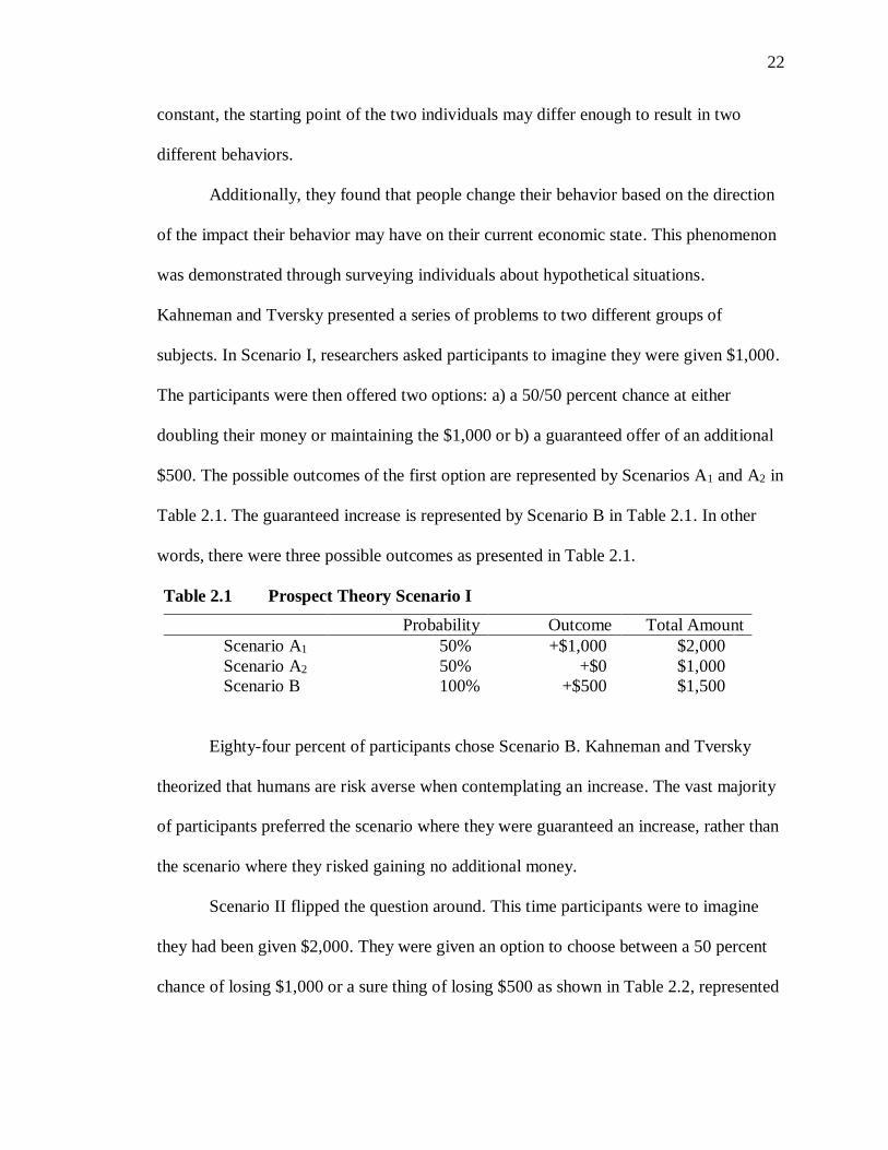
Additionally, they found that people change their behavior based on the direction
of the impact their behavior may have on their current economic state. This phenomenon
was demonstrated through surveying individuals about hypothetical situations.
Kahneman and Tversky presented a series of problems to two different groups of
subjects. In Scenario I, researchers asked participants to imagine they were given $1,000.
The participants were then offered two options: a) a 50/50 percent chance at either
doubling their money or maintaining the $1,000 or b) a guaranteed offer of an additional
$500. The possible outcomes of the first option are represented by Scenarios A1 and A2 in
Table 2.1. The guaranteed increase is represented by Scenario B in Table 2.1. In other
words, there were three possible outcomes as presented in Table 2.1.
Table 2.1 Prospect Theory Scenario I
Probability Outcome Total Amount
Scenario A1 50% +$1,000 $2,000
Scenario A2 50% +$0 $1,000
Scenario B 100% +$500 $1,500
Eighty-four percent of participants chose Scenario B. Kahneman and Tversky
theorized that humans are risk averse when contemplating an increase. The vast majority
of participants preferred the scenario where they were guaranteed an increase, rather than
the scenario where they risked gaining no additional money.
Scenario II flipped the question around. This time participants were to imagine
they had been given $2,000. They were given an option to choose between a 50 percent
chance of losing $1,000 or a sure thing of losing $500 as shown in Table 2.2, represented

23
by the two possible outcomes to the chance proposal in Scenarios C1 and C2 or the
guaranteed decrease in Scenario D.
Table 2.2 Prospect Theory Scenario II
Probability Outcome Total Amount
Scenario C1 50% -$0 $2,000
Scenario C2 50% -$1,000 $1,000
Scenario D 100% -$500 $1,500
The odds and the final amounts in Scenario II are exactly the same as those
presented in Scenario I. In both questions, the individuals choosing Scenarios A or C
have a 50 percent chance of a final amount of $2,000 and a 50 percent chance of a final
amount of $1,000. Scenarios B and D both result in the individual walking away with
$1,500. The only difference is the starting point, or reference point, which determines the
value (positive or negative) of the choice. In the Scenario II, 69 percent of participants
chose Scenario C, indicating risk seeking. The participants to this question demonstrated
that when faced with a loss, they were more likely to choose a potential large loss if it
also meant there was a chance that they would lose nothing.
Kahneman and Tversky argued that the survey responses provided evidence that a
$500 gain is different than a $500 loss. They argued that their evidence suggested that
individuals view losses as nearly twice as impactful as a gain. This meant that the slope
of the line is steeper on the losses end of the graph. Moreover, they argued that when an
individual’s starting point is high, for example $2,000, a $100 change is not valued the
same as if the starting point is low. Therefore, at both ends of the graph the line is
asymptotic as gains are still viewed as positive and losses are viewed as negative, but
diminishing returns mean that those gains and losses are less impactful. They displayed
the plotted data as “The Value Function” (Figure 2.1).

24
Figure 2.1 Value Function (Kahneman & Tversky, 1979)
Other researchers have used Prospect Theory to examine a variety of situations.
Fryer, Levitt, List, and Sadoff (2012) and Levitt, List, Neckerman, and Sadoff (2016)
found that both teachers and students react differently to positive and negative stimuli. In
both of these studies, teachers and students display a greater effort when monetary
increases are framed as losses rather than gains. These findings are consistent with those
of Kahneman and Tversky in that the perceived magnitude of a loss is greater than the
perceived benefit of gains and that individuals value a good more when they must give it
up than when it can be acquired (Kahneman, Knetsch, and Thaler, 1990; Fehr, Goette,
and Zehnder, 2007).
Simon, displaying his role as a sort of academic prophet wrote, “human rationality
operates, then, within the limits of a psychological environment” (1997, p. 117). The
original printing of Simon’s book, Administrative Behavior, was published in 1947, long
before Kahneman and Tversky developed Prospect Theory.
The Endowment Effect
Kahneman and Tversky’s disciple Richard Thaler used a list of “irrational”
human behaviors to explore explanations for those behaviors (Thaler, 2015). The result
was the “Endowment Effect” (Thaler, 1980).

25
Thaler, like Kahneman and Tversky, saw behaviors that were irrational. He
describes one scenario in which a person buys a case of wine for $5 per bottle. Years
later, a wine merchant offers to buy the wine for $100 per bottle. Although the individual
has never paid more than $35 for a bottle of wine, the person refuses to sell. Later, Thaler
reveals that this scenario was based on actual events (Thaler, 2015). Although the wine
was purchased at only $5 per bottle, the wine has become more valuable to the owner. It
has become so much more valuable, that the owner refused to sell the wine for $100 per
bottle. He wanted to understand why an individual would be unwilling to sell a good that
he owns for more than its original purchase price. Thaler theorized that the value of a
good increases once it becomes part of the owner’s endowment (Thaler, 1980). An
experiment was developed with college coffee mugs (Kahneman, Knetsch, & Thaler,
1990).
The researchers provided college coffee mugs to approximately half of a class.
Students who received a mug were able to identify the price at which they would be
willing to sell their mug, i.e., willingness to accept. Students without a mug were able to
identify the price at which they would be willing to purchase a mug, i.e., willingness to
pay.
Researchers found a significant difference in the amount of money students were
willing to accept and the amount of money students were willing to pay. The students
who were given a coffee mug valued the mug at much higher levels than the students
who were not given a mug (see Table 2.3).

26
Table 2.3 Endowment Effect Experiment
Trial Median Buyer
Reservation Price
Median Seller
Reservation Price
4 $2.75 $5.25
5 $2.25 $5.25
6 $2.25 $5.25
7 $2.25 $5.25
Kahneman, Knetsch, and Thaler (1990) argued that the value of a good increases
the moment the individual is given the object. The researchers claim, “the act of giving
the participant physical possession of the good results in a more consistent endowment
effect. Assigning subjects a chance to receive a good, or a property right to a good to be
received at a later time, seemed to produce weaker effects” (p. 1342).
Explaining Citizen Behavior
The combining of public administration and behavioral economics is becoming
more widely accepted and studied. This is evidenced by the actions of the United
Kingdom creating the Behavioral Insights Team in 2010 and with President Obama’s
2015 executive order launching the Social and Behavioral Sciences Team. The goal of
these teams is to develop a deeper understanding of the cognitive limitations of citizens
and to better predict how citizens will behave, thus combining the actions of government
with the theory of behavioral economics. The hope is that these teams could develop
initiatives that are psychologically based and will encourage citizens to adopt desired
behaviors (Grimmelikhuijsen, Jilke, Olsen, and Tummers, 2017; Madrian, 2014).

27
The intersection of public policy and behavioral economics has recently been
used to inform public administration research (Rabin, 1998; Thaler and Sunstein, 2008;
Congdon, Kling, and Mullainathan, 2011). For example, Dynarksi and Scott-Clayton
(2006) demonstrated that program participation rates are affected by the simplicity level
of an enrollment process and that complexity acts as a barrier to potential participants.
Currie (2004) found that automatic enrollment processes increased participation rates in
401(k) retirement-savings programs and Medicare. Participants were less likely to forego
enrollment if that enrollment was automatic. Both studies suggest that if the goal of an
initiative is to increase the participation of a program, behavioral economics would
encourage simplifying the admission process, up to the point of automatic enrollment into
the program, as a method for increasing participation rates (Babcock, Congdon, Katz, and
Mullainathan, 2012).
In another use of behavioral economics to explain citizen behavior, differences in
food labeling were studied by Berg (2003). Berg noted that labeling the cholesterol
content of food is costly to the food producer and provides information readily available
elsewhere. Despite the cost and redundancy of information, Berg suggested that
Behavioral Economics dictates that labeling the cholesterol content of food may actually
encourage consumers to purchase that food. The benefit comes from offering the
immediate availability of the cholesterol content to the consumer in an overloaded
information environment (Berg, 2003).
Behavioral Economics of Students
The foregoing discussion suggests that simplifying a process every incoming
college student must undertake, i.e. being accepted to college, would incentivize college

28
enrollment among students. Thaler (2015) noted that these types of policies are meant to
reduce transaction costs, “mak[ing] it easier for people to make what they will deem to be
a good decision, both before and after the fact, without explicitly forcing anyone to do
anything” (p. 324).
The Role of Value
Increasing the ease of a process is one possible incentive to behave in a way that
revises one’s state of affairs. Valuing the process and its outcome is another. In The
Administrative State, Waldo (1948) describes the subject matter of economics as the,
“‘valuations,’ given introspectively for single individuals. Since individuals
differ, a different ‘science of economics’ might result for each person… Administrative
study, as any ‘social science,’ is concerned primarily with human beings, a type of being
characterized by thinking and valuing. Thinking implies creativeness, free will. Valuing
implies morality, conceptions of right and wrong” (p.181).
In other words, the behavior of individuals is based on the value they place on the
outcome of one behavior over another. For graduating high school seniors, the relative
value they place on college may impact their enrollment. Behavior may be driven by the
value of attending college or not; attending one college over another; seeking one field of
study over another; accruing credits quickly or slowly; or pursuing one level of degree
over another. If the substantial money college costs is valued more than college itself, the
graduating high school senior is less likely to enroll in college, particularly given the
more than five years now required, on average, to complete a baccalaureate degree
(Shapiro, Dundar, Wakhungu, Yuan, Nathan, & Hwang, 2016).
Past research suggests that factors such as race, gender, urbanicity, and
socioeconomic status may also impact the value students place on college (Adelman,
2002; Averett & Burton, 1996; Black & Sufi, 2002; Cabrera & La Nasa, 2000; Goldin,

29
Katz & Kuziemko, 2006; Gose, 1999; Hurtado, Inkelas, Briggs, & Rhee, 1997; Light &
Strayer, 2002; McFarland, J. et al., 2018; Wagner & Blackorby, 1996; Thomas, 1980).
Another factor that plays a role in college attendance behavior is the highest level of
education earned by the student’s parents (Pascarella, Pierson, Wolniak, & Terenzini,
2004; Terenzini, Springer, Yaeger, Pascarella, & Nora, 1996). In Idaho, white students
enroll at higher rates than Hispanic students, Native American students enroll at lower
rates than other racial groups, and females enroll at higher rates than males (McHugh,
2015). Students in eastern Idaho enroll in college at lower rates than the state average,
presumably because of the high population of adherents to The Church of Jesus Christ of
Latter-day Saints who serve religious missions (McHugh, 2015). In sum, whether
graduating high school students value college over other alternatives may be impacted by
these or a variety of any number of other factors. Prospect Theory and/or The
Endowment Effect may be useful in anticipating what values graduating high school
seniors bring to the notion of enrolling in college.
Direct Admissions and Prospect Theory
Under Direct Admissions, Idaho high school seniors are notified that they qualify
for admission at either six or eight Idaho colleges, depending on their level of academic
achievement as measured by high school grade point average and college entrance
examination scores. Prospect Theory, in this instance, regards whether college-bound
students will take the sure bet (acceptance at an Idaho public institution) or risk time and
money waiting for an offer from a competing college. Students not subject to Direct
Admissions who apply to a college and pay the application fee are taking a risk. They
must wait to see, for example, if their grades are high enough, if their essay is good

30
enough, or if their civic engagement activities are compelling enough for acceptance.
Students often do not know until they apply whether they have met the criteria necessary
for acceptance. Under Direct Admissions, students know, in advance, which institutions
have accepted them. Under Prospect Theory, students would be predicted to take the sure
thing and not risk the negative experience (not being accepted elsewhere) that Kahneman
and Tversky (1979) claim has twice the impact of a positive experience.
Direct Admissions and The Endowment Effect
The original study resulting in development of The Endowment Effect examined
the value of a coffee mug once that mug was possessed by an individual. In this research,
at the moment of possession, mugs became more valuable to individuals than they had
been before they received them. In the case of graduating high school seniors, if students
have been accepted to a college and if they express a sense of ownership over that
acceptance, the offer may become more valuable than alternative offers or other options.
These options and alternatives, the Endowment Effect claims, would have to provide
more value to students to accept a trade. Direct Admissions may induce a sense of
ownership over acceptance to Idaho colleges that students may not wish to lose by
accepting an alternative.
Direct Admissions changes very little in the actual admissions process. Students
who were eligible for acceptance in the Group of 8 colleges would most likely have been
eligible for acceptance to those same schools had the initiative not been implemented.
Direct Admissions does not allow students to attend college for free, nor does it penalize
students who choose not to attend. Other than eliminating the application fee, the cost of
college would be the same with or without Direct Admissions. Admissions standards

31
collaboratively developed by institution provosts, are similar to the standards that
preceded implementation of the program. Direct Admissions and its messaging campaign
from the Idaho State Board of Education, was designed to increase the perceived value of
college. Prospect Theory and the Endowment Effect theorize that students receiving a
Direct Admissions letter would be encouraged to enroll in an Idaho public college as that
acceptance letter becomes more valuable relative to other college options. Additionally,
the magnitude of influence of the Direct Admissions letter would be correlated with the
relative starting point of the individual’s attitude towards college.
In the next chapter, I discuss the methodology for this study. I present the
argument for utilizing a linear probability model, the variables used in the model, and
limitations of this model. I also explain the survey instrument used to collect student
attitudes on the Direct Admissions letters and describe the limitations of the instrument.

32
CHAPTER THREE: METHODOLOGY
Research Design and Methods
This study into whether Direct Admissions correlates with student enrollment
behavior employed a mixed-methods approach involving both quantitative and
qualitative data collection and analysis. A quantitative approach allowed me to estimate
the overall magnitude of the effect of the initiative. The collection and analysis of
qualitative data allowed me to better understand student views on the influence Direct
Admissions has on enrollment. Quantitative and qualitative data were both collected at
the student level. Data collection methods, procedures, and limitations are described
below.
Data Sources
When a student enrolls at any level of education in Idaho, an Educational Unique
Identifier (EDUID) is generated for that student. Each EDUID follows the student
through public education and, when applicable, into and through Idaho’s public
postsecondary institutions. If the student is in primary or secondary school, that EDUID
is uploaded to the Idaho State Department of Education along with course enrollment and
demographic information, which includes: race, ethnicity, gender, and free or reduced-
price lunch status (FRPL). That information, for all public traditional and charter schools,
is stored in the Educational Analytics System of Idaho (EASI) and updated by the schools
five times each school year.

33
For this study, individual student-level data were collected from EASI. These data
are housed indefinitely and allow authorized individuals to look at longitudinal trends in
education, including the transition from public K-12 to higher education.
A separate database within EASI stores student-level data collected from each of
the public postsecondary institutions in the state as well as enrollment information from
private and out-of-state postsecondary institutions using information provided by the
National Student Clearinghouse (NSC). The NSC is a national database that collects
enrollment and completion information for all postsecondary institutions that are eligible
for receiving federal financial aid.
Each individual school district in Idaho uploads the data on K-12 students to the
Idaho Department of Education, which then passes it to the Idaho State Board of
Education in order to calculate the Direct Admissions benchmark score for each student.
These scores are calculated by reviewing a student’s transcript and calculating a GPA
based on the letter grades the student received and the number of credits a student has
earned. College entrance exam scores are collected directly from the vendors that
administer those tests. Through agreements with each of these vendors, the Idaho State
Board of Education collects the student-level results of these exams.
For this study, I created a single database that combines the demographic
information uploaded to the Idaho Department of Education and the college entrance
exam scores collected by the Idaho State Board of Education. This information was
accessible because of my role as the Chief Research Officer. Because Idaho state law
prohibits the collection of religious affiliation data into EASI, I was not able to collect
student-level religion data. I included the high school the student attended and county
34
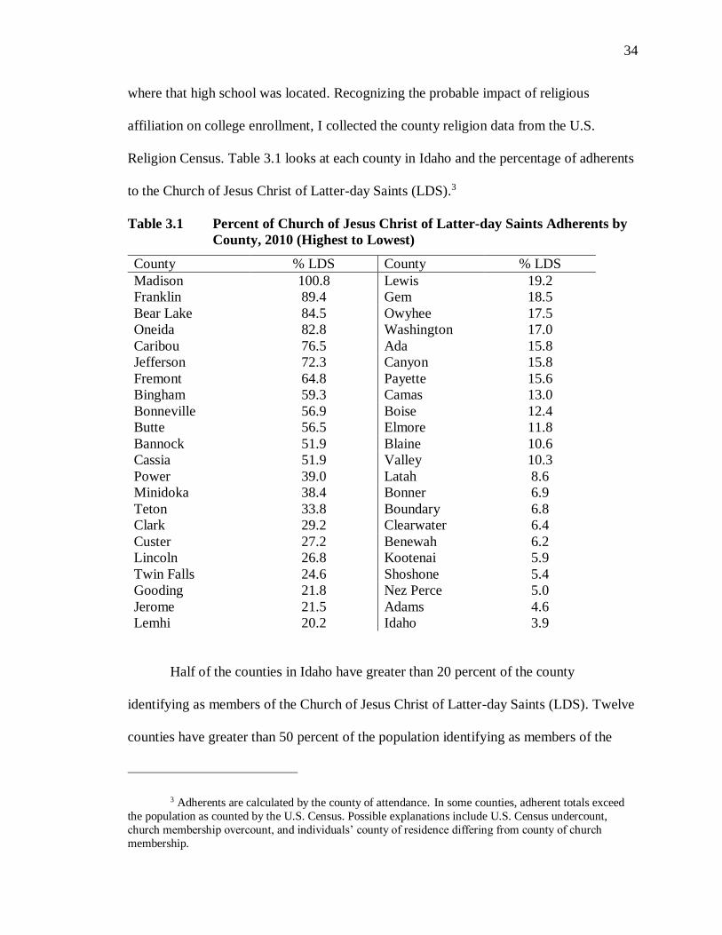
where that high school was located. Recognizing the probable impact of religious
affiliation on college enrollment, I collected the county religion data from the U.S.
Religion Census. Table 3.1 looks at each county in Idaho and the percentage of adherents
to the Church of Jesus Christ of Latter-day Saints (LDS).3
Table 3.1 Percent of Church of Jesus Christ of Latter-day Saints Adherents by
County, 2010 (Highest to Lowest)
County % LDS County % LDS
Madison 100.8 Lewis 19.2
Franklin 89.4 Gem 18.5
Bear Lake 84.5 Owyhee 17.5
Oneida 82.8 Washington 17.0
Caribou 76.5 Ada 15.8
Jefferson 72.3 Canyon 15.8
Fremont 64.8 Payette 15.6
Bingham 59.3 Camas 13.0
Bonneville 56.9 Boise 12.4
Butte 56.5 Elmore 11.8
Bannock 51.9 Blaine 10.6
Cassia 51.9 Valley 10.3
Power 39.0 Latah 8.6
Minidoka 38.4 Bonner 6.9
Teton 33.8 Boundary 6.8
Clark 29.2 Clearwater 6.4
Custer 27.2 Benewah 6.2
Lincoln 26.8 Kootenai 5.9
Twin Falls 24.6 Shoshone 5.4
Gooding 21.8 Nez Perce 5.0
Jerome 21.5 Adams 4.6
Lemhi 20.2 Idaho 3.9
Half of the counties in Idaho have greater than 20 percent of the county
identifying as members of the Church of Jesus Christ of Latter-day Saints (LDS). Twelve
counties have greater than 50 percent of the population identifying as members of the
3 Adherents are calculated by the county of attendance. In some counties, adherent totals exceed
the population as counted by the U.S. Census. Possible explanations include U.S. Census undercount,
church membership overcount, and individuals’ county of residence differing from county of church
membership.

35
LDS church. On the other end of the spectrum, ten counties have fewer than 10 percent of
the county identifying as members of the LDS church. The distribution of members of the
LDS church suggests that in certain parts of the state, members of the LDS church are
more tightly clustered together. It is assumed that a similar distribution of membership in
the LDS church at the county level is seen in the high school. In the quantitative analyses,
controlling for the high school the student attended would also control for the fixed
effects of that high school, including the religious distribution of the students. The county
in which the high school is located is therefore used in this study as a control variable for
religious affiliation. This control is done by using the high school number assigned by the
Idaho State Department of Education.
Idaho public colleges collect individual student data including the student’s name,
date of birth, and previous high school when a student applies. I used these data from the
postsecondary institution to match back to the student’s EDUID and the Direct
Admissions letter the student received. I used the Idaho Department of Education
designation of each school as an urban or rural school. This process allowed me to match
a student’s enrollment and attendance at a college or university to the demographic
information collected by the State Department of Education and the Direct Admissions
letter benchmark score developed by the Idaho State Board of Education. I deleted the
EDUIDs and generated a unique research identifier so that the students in the data set
could not be reidentified.
The data elements collected are listed in Table 3.2. The table lists each of the data
variables, the unit of analysis for that data variable, and the structure of those data used
for this analysis. Each of these variables are further described in the next section. That

36
section also describes how the analytical models I used for this study utilize these
variables.
Table 3.2 Variables, Variable Level, and Variable Types
Variable Variable Level Variable Type
Enrolled Student Dichotomous
Direct Admissions Letter Student Dichotomous
Lunch Status (Not free or reduced-
price, Free or reduced-price) Student Dichotomous
Gender Student Dichotomous
Race/Ethnicity (Non-white, White) Student Dichotomous
Urbanicity School/Student Dichotomous
High School Number School/Student Categorical
In addition to the quantitative data collected, I developed and conducted a survey
of students who received their Direct Admissions letter. The electronic survey was sent to
all students who applied to an Idaho public postsecondary institution prior to the
February 15 deadline (see Appendix A). In assessing the influence of the Direct
Admissions letter on a student’s behavior, I desired to know how much of an influence it
had on the first step toward enrolling in an Idaho college -- application. Names of
students who did not apply to Idaho colleges or who applied exclusively to out-of-state
institutions were removed from the data set and did not receive the survey for this study.
The survey sample included only those students who had applied to enroll in a public
Idaho postsecondary institution.
Methods – Quantitative
I begin with a summary of observed behaviors. The Idaho State Board of
Education collects from the institutions a summary of in-state students who applied to
their institution in previous years. Through an analysis of these data and comparison of
the 2013, 2014, 2015, and 2016 high school graduating classes, I can determine if there

37
has been a significant change in the number of students who enrolled at an in-state public
institution after receiving a Direct Admissions letter compared to the enrollments in
previous three years. Since many of the institutions have participated in a number of
strategies to increase enrollment, any significant change cannot be wholly attributable to
Direct Admissions. A significant change between the years, however, could suggest that
Direct Admissions is correlated with student enrollment behavior.
For the quantitative section of the analysis, I utilize a series of regression models
to estimate the impact of Direct Admissions in a student’s enrollment in college. The
regression models are a series of linear probability models (LPM). The LPM was selected
in lieu of probit or logit models because of the ability to estimate group variables by LPM
(Caudill, 1988). A group variable is where an entire group exhibits or does not exhibit the
behavior in question. If all Group of 8 recipients applied to college, or if all or none of the
students exhibiting other characteristics applied to college, the coefficient of that
independent variable cannot be estimated through a probit or logit model.
I calculate the percentage of enrolled students on each of the independent
variables. This measure becomes the “non-adjusted difference” between the two groups
on the independent variable in question. I then run a LPM, including the Direct
Admissions letter variable as an interaction variable with the independent variable in
question and controlling for other characteristics. The coefficient of this output becomes
the “adjusted difference”. Comparing the non-adjusted difference and the adjusted
difference suggests whether the inclusion of Direct Admissions is positively correlated
with enrollment behavior. If the adjusted difference is closer to zero than the non-
adjusted difference, the results would suggest Direct Admissions is positively correlated

38
with enrollment behavior. If the adjusted difference is farther from zero, meaning that the
enrollment gap between the two groups had gotten larger, the results would suggest that
Direct Admissions is negatively correlated with enrollment behavior.
The series of regressions estimate the non-adjusted and adjusted differences in
enrollment behavior of select characteristics of students. The output from these
regressions suggest, or do not suggest, that Direct Admissions is positively correlated
with college enrollment behavior. The dependent variable is binary. The dependent
variable is whether a student has enrolled at one of the Idaho public institutions or not.
Enrollment is determined by matching the spring 2016 high school graduating student to
the fall 2016 college enrollment records at any of the Idaho public colleges or
universities. The independent variables are which letter the student received (Group of 6
or Group of 8), free or reduced-price lunch (as an indicator of poverty), gender,
race/ethnicity, urbanicity of the school, and the student’s high school.
Linear Probability Model Regression on College Enrollment
The linear probability model employed looks at the variables that influence
college enrollment. I include a variable on the Direct Admissions letter type the student
received and then a series of controls. With the exception of the high school the student
attended, the controls are also used in subsequent models as a moderator for the model.
Enrollment = α + β1*(Direct Admissions Letter Type) + β2*(Moderator) +
β3*(Direct Admissions)*(Moderator) + B’(Vector of Controls)
The moderators for the model are Free or Reduced-Price Lunch Status (as a proxy
for socioeconomic status), Gender, Race/Ethnicity, and Urbanicity. Interaction terms

39
calculate the impact of a particular moderator with the Direct Admissions letter type
(Group of 8 or Group of 6 letter).
In each model, each interactive variable is included as a control, with the
exception of urbanicity – for example, in Model 1, Free or Reduced-Price Lunch Status is
the moderator, but gender and race/ethnicity are included as control variables.
Additionally, fixed effects for high school are included in all models, with the exception
of Model 5, as high school is correlated with urbanicity.
College Enrollment is a binary dependent variable based on whether the student
who received a Direct Admission letter enrolled in college.
Direct Admissions Letter Type is a dummy variable indicating whether the
student received a Group of 6 letter or a Group of 8 letter, meaning how many institutions
were identified in the student’s letter as already accepting the student.
Lunch Status is a dichotomous variable that indicates the student’s federal lunch
program participation. Free or reduced-price lunch is often used as a proxy variable
reflecting a student’s family income (Koffman & Tienda, 2008). This variable was
selected in an effort to be conservative in the estimation of free or reduced-price lunch. A
student may be eligible for the federal school lunch program as a senior in high school,
but may perceive a negative stigma attached to the program and decline participation. For
this reason, I chose to calculate this variable by whether a student has ever qualified for
the program. A student is categorized as either receiving free or reduced-price lunch or
not.

40
Students who were enrolled at a school that is classified as a Community Eligible
Provision4 (CEP) school are also included. This could lead to potentially overestimating
the poverty since schools receiving the Community Eligible Provision provide 100
percent of their students with free school lunch, regardless of individual eligibility.
Relying solely on lunch eligibility status, there could be students who might be classified
as low socioeconomic status when their participation in the program is more dependent
on the school they are attending rather than their economic situation. However, the
converse is also true in situations where students who may be eligible for free or reduced-
price lunch do not claim those benefits. I assume, for purposes of this study, that those
characteristics are equally distributed across high schools.
Gender is also a dummy variable that indicates whether the student is male or
female.
Race/Ethnicity is a dummy variable that indicates whether the student is white or
non-white. Idaho is a relatively homogenous state with a small percentage of non-white
residents. Rather than break each racial or ethnic group into its own category, I chose to
have a dichotomous variable indicating whether the student is white or non-white.
High School is a categorical variable that is used to control for factors such as
religion and urbanicity. An important factor to note is Idaho has a relatively high
population of adherents to the Church of Jesus Christ of Latter-day Saints (LDS). Among
4 A Community Eligible Provision (CEP) is granted to schools and school districts in low-income areas. CEP allows the highest poverty schools and districts to serve breakfast and lunch at no cost to all
enrolled students without collecting household applications. Instead, schools that adopt CEP are reimbursed
using a formula based on the percentage of students categorically eligible for free meals based on their
participation in other specific means-tested programs, such as the Supplemental Nutrition Assistance
Program (SNAP) and Temporary Assistance for Needy Families (TANF).

41
the LDS culture, young men at the age of 18 and young women at the age of 19 are
strongly encouraged to serve a religious service mission for the church. These missions
last for up to two years and are typically fulfilled away from an individual’s home. This
means that for these LDS men, college enrollment, when it occurs, is usually delayed
until at least age 20. For LDS women, college enrollment may be delayed if the young
woman intends to serve a religious mission and attend college upon completion of the
missionary service. This behavior will influence the results of the analysis since the letter
will have appeared to have no effect, but could be a result of the student’s religious
affiliation and not the failed impact of the Direct Admissions letter. Approximately 25
percent of Idaho self-identifies as a member of the LDS church. This substantial number
means that college enrollment could have been affected due to mission behavior.
In addition to the variables seen in the other models, Model 4 and Model 5
contain a variable for urbanicity. The urbanicity of the school is the classification of the
school as reported by the Idaho State Department of Education. This dichotomous
variable indicates whether the student attended a rural or not-rural high school. This
variable is included separately in an effort to break out the influence of urbanicity on
enrollment without the influence of religion.
Methods – Survey of Students
I developed a survey to be answered by students who had applied to college after
receiving their Direct Admissions letters. The survey was developed within the Idaho
State Board of Education and through my role as the Chief Research Officer. The
purpose of the survey was to evaluate the influence the Direct Admissions letters had on
the behavior of the students.

42
I emailed the survey in March 2016 to all students who applied to an Idaho public
college or university. I sent two follow-up emails as reminders for students to complete
the survey. I sent the survey to 8,343 students who had applied to college by the February
15 deadline indicated in the student’s Direct Admission letter. I received responses from
1,410 students, for a response rate of 17 percent.
The survey was anonymous, although the student’s high school was asked. The
surveys were sent electronically to the students directly. This was done to collect a
geographically representative sample and not be limited by a school who may have
refused to participate.
In an effort to not compromise anonymity of students, defining characteristics
such as race or ethnicity were not collected in the survey instrument. While the sample
may be geographically representative, it may not be demographically representative.
Since the survey was anonymous, there was no ability to connect the survey responses to
the student data used in the quantitative analysis.
I asked students to rate on a 1-5 scale the impact the Direct Admissions letter had
on the student’s behavior in applying for college. I also asked the students to use the
same scale to evaluate how much of an impact the Direct Admissions letter had on their
behavior of applying to a particular college. After each rating, the students could explain
their answers in an open answer text. I coded the open text answers through looking for
common themes that emerged among the students that indicated the Direct Admissions
letter had a positive impact, no impact, or negative impact.
The survey was designed to allow students to select answers from a drop-down
list and also provide open-text answers. The limited-selection answers could be used for

43
general scoring. I coded the open-text answers to look for emerging themes. Coding the
responses was completed using conventional content analysis (Hsieh & Shannon, 2005). I
was able to consider the answers the student provided to both the scale score and the
open-text answer. This was not done to try and catch the student providing differing
answers, but was done to help better understand the student’s behavior. For example, if
the student indicated that Direct Admissions had no impact on their behavior to attend
college and then provided an open-text answer about how the student had always planned
on going to college but decided to stay in Idaho for college after receiving the letter, I
was able to code that response as the Direct Admissions letter had a positive impact. The
letter may not have influenced the student’s desire to attend college, but the letter
appeared to have an impact on the student’s behavior to attend an Idaho college.
Coding was done by reading both the scale score the student provided and the
open-text response. If either response indicated a positive impact, the entire survey
response was coded as positive impact. The same was done for surveys that were coded
as no impact, or negative impact. The coded impacts were then clustered together and re-
evaluated to ensure correct coding (Saldana, 2013).
Limitations of Study
There are limitations to both this particular study and the replication of this study.
One limitation that is present within the study is the quality of the data, both the
quantitative data and the survey data. Each student receives a unique student identifier
(EDUID). That EDUID is used as the student transitions from high school to college. If
the college does not use the same EDUID for that student that the student had in high
school, that student will be coded as not enrolling in college. The result of this error

44
would mean that the number of students identified as enrolling in college would be lower
than the actual number. Historical corrections of the enrollment data suggest that this
error could impact the go-on rate by up to approximately three percentage points. It is
unlikely that false positives would be identified, meaning that a college would incorrectly
identify a student as enrolling that was not on campus. It should be noted that while the
data are collected in a consistent manner, the process has also improved over time.
Therefore, any errors would be consistent with data from prior years, if those errors in
data collection have not already been corrected.
Another quantitative limitation is the free or reduced-price lunch data. Students
attending a Community Eligible Provision (CEP) school are identified as receiving free
or reduced-price lunch. However, since I am using lunch status as a proxy variable for
income, students who are above the income threshold for free or reduced-price lunch
would be incorrectly identified as low income because of the provision the school district
was granted. In order to correctly identify students who would otherwise be counted as
incorrectly eligible for benefits or even incorrectly not eligible for benefits, I would need
access to individual student’s, or the student’s family’s, tax documents. Those data were
not available for this study.
The survey used for this study was developed internally at the Idaho State Board
of Education. This survey was not designed from extant nationally normed instruments
that had gone through exhaustive psychometric testing. This could impact the validity
and reliability of the survey instrument itself. This was the first time that the survey had
been conducted, so there was no historical data to which I could compare the responses.

45
There are several characteristics that could limit the applicability or
generalizability of this study to other states, other students, and other education systems.
Idaho has a unique governing structure that is only shared with Rhode Island, where the
State Board of Education governs both the public K-12 and the higher education systems.
Idaho was able to implement this initiative, in part due to the unified governance over the
educational systems and the access to student data across the different levels of
education.
Idaho is a rural state that has a low go-on rate. In a larger state where there are
more graduating high school students, a highly selective college, or a very popular
college, the availability of a campus to absorb what could be a large influx of students
could be prohibitive to other states or education systems from adopting this initiative.
In the next chapter, I discuss the quantitative analysis performed. I present the
output from the linear probability model and discuss the findings. I interpret if the
findings suggest that Direct Admissions is positively correlated with student enrollment
behavior for each of the subgroups identified.

46
CHAPTER FOUR: QUANTITATIVE RESULTS
Enrollment Trends
This chapter begins with a comparison across time of the graduating high school
classes and their enrollment numbers in Idaho public colleges (see Table 4.1). The second
year of the academic year indicates the year of a class (e.g., students who were in their
last year of high school during 2012-2013 are the class of 2013). The high school
graduating class of 2013 saw 45.1 percent of the students enroll in an Idaho public
college in the fall semester immediately following high school graduation. That number
gradually decreased for the years reported. The high school graduating class of 2016 was
the first class that received the Direct Admissions letters. This class saw a go-on rate of
41.8 percent.
Table 4.1 Fall Immediate Enrollment Trends at Idaho Public Colleges,
Academic Years of High School Graduates 2012-2013 through 2015-
2016
2012-2013
2013-2014
2014-2015
2015-2016
Total Students 19,236 20,255 19,932 19,353
% Enrolled
Total Students 45.1% 43.9% 42.4% 41.8%
Total Not
Free Lunch 12,352 13,002 12,987 12,020
% Enrolled
Not Free
Lunch
50.9% 49.6% 47.7% 48.5%

47
Total Free or
Reduced
Lunch
6,884 7,253 6,945 7,333
% Enrolled
Free or
Reduced
Lunch
34.7% 33.6% 32.6% 30.8%
Total Male 9,677 10,267 10,208 10,036
% Enrolled
Male 35.8% 36.2% 35.3% 33.8%
Total Female 9,559 9,988 9,724 9,317
% Enrolled
Female 54.5% 51.8% 49.9% 50.4%
Total White 15,396 16,001 15,752 15,040
% Enrolled
White 46.6% 45.2% 43.4% 42.8%
Total Non-
White 3,840 4,254 4,180 4,313
% Enrolled
Non-White 39.1% 39.0% 38.8% 38.3%
Total Rural 7,353 7,446 7,285 7,371
% Enrolled
Rural 42.7% 41.3% 39.4% 38.1%
Total Not
Rural 11,883 12,809 12,647 11,982
% Enrolled
Not Rural 46.6% 45.4% 44.2% 44.0%
The overall rates do not show a large increase in go-on rates. In fact, many of the
rates decreased from 2014-15. Increases were only seen in the female enrollment and the
enrollment of students who were not classified as receiving free or reduced-price lunch.
Only the changes for male students and students receiving free or reduced-price lunch

48
were found to be significant from 2014-15 to 2015-16. Both of those were decreases in
2015-16 and were significant at the p<0.05 level (Table 4.2).
Table 4.2 T-test of Significance of Enrollment for Academic Years 2014-15 and
2015-16
Variable (2014-15 data in parentheses) Mean Std. Dev. df t p
Total enrollment
(0.424)
0.418
(0.499)
0.500 39,283 1.34 0.18
Free or reduced-price lunch enrollment
(0.326)
0.308
(0.469)
0.462 14,276 2.30 0.02**
Not free or reduced-price lunch
enrollment
(0.477)
0.485
(0.004)
0.005 25,005 -1.20 0.23
Male enrollment
(0.353)
0.338
(0.478)
0.473 20,242 2.22 0.03**
Female enrollment
(0.499)
0.504
(0.500)
0.500 19,039 -0.57 0.57
White enrollment
(0.434)
0.428
(0.496)
0.495 30,790 1.12 0.26
Non-white enrollment
(0.388)
0.383
(0.487)
0.486 8,491 0.50 0.62
Rural enrollment
(0.394)
0.381
(0.489)
0.486 14,654 1.58 0.11
Non-rural enrollment
(0.442)
0.440
(0.497)
0.496 24,627 0.28 0.78
*p < 0.1 **p < 0.05 ***p < 0.01
While the historical view of enrollment and the t-test significance provides
context to the analysis, the question of if Direct Admissions is correlated with the
enrollment behavior of students cannot be answered through Table 4.2. As presented in
Chapter 3, this analysis utilizes a linear probability model to estimate the impact of the
interaction of the Direct Admissions letters with the different subgroups. Other variables
are used as control variables. The analysis is done using only the 2015-16 high school
graduating class as this was the first year that the Direct Admissions letters were provided
to students.

49
Variables
The variables in this analysis are presented in Table 4.3. The records of 19,353
students were accessed for this study and, with exception of High School Number, a
categorical variable, all the variables are dichotomous. Religious adherence, collected at
the county level by the U.S. Religion Census is displayed in Table 3.1, showed the
clustering of LDS adherents by county. The high school number variable is used to
control for the LDS population (U.S. Religion Census, 2010).
Table 4.3 Summary of Variables, Student Enrollment Fall 2016
Variable Mean Std. Dev Min. Max. n
Enrollment (Yes=1, No=0) 0.418 0.493 0 1 19,353
Direct Admissions Letter
(Group of 8=1, Group of
6=0) 0.529 0.499 0 1 19,353
Free or Reduced-Price
Lunch (Not Free or
Reduced=1, Free or
Reduced=0) 0.621 0.485 0 1 19,353
Gender (Male=1,
Female=0) 0.519 0.500 0 1 19,353
Race/Ethnicity (White=1,
Non-White=0) 0.777 0.416 0 1 19,353
Urbanicity (Rural=1, Not
Rural=0) 0.381 0.486 0 1 19,353
High School Number 420.450 974.033 7 9,034 19,353
Since I am interested in the correlation of these variables with the Direct
Admissions letters, I looked at the differences in enrollment behavior across each of these
variables and tested the interaction of the Direct Admissions letters with each variable,
while holding other variables constant.
General Statistics of Variables
Prior to running the regression models, I ran a crosstab analysis on the
relationship between the Direct Admissions letters and each variable. The first variable

50
included in the model was free or reduced-price lunch status. Since individual poverty-
level information was not available for this analysis, free or reduced-price lunch status
was used as a proxy for individuals’ poverty-level information. Students who receive free
or reduced-price lunch are one category, while the other category contains those students
who receive no subsidy on their school lunch. Table 4.4 presents the relationship of each
variable with both types of Direct Admissions letters. Since each of the variables are
looked at independently, the percentages included in Table 4.4 are looked at
independently. For example, 23.8 percent of all students were classified as receiving free
or reduced-price lunch and also got a Group of 6 letter. This allows the percentages to be
summed across demographics. All the free or reduced-price lunch students accounted for
38.0 percent (adding the Group of 6 and Group of 8 letter columns). The high school
variable is not included as it is used as a control variable by each individual high school.
Table 4.5 presents the Pearson Chi-Square results for statistically significant
relationships.

51
Table 4.4 Crosstabs of Free or Reduced-Price Lunch and Direct Admissions
Group of 6 Letter Group of 8 Letter
Free or Reduced-Price Lunch 4,609
(23.8%)
2,724
(14.2%)
Not Free or Reduced-Price
Lunch
4,507
(23.3%)
7,513
(38.8%)
Female 3,662
(18.9%)
5,655
(29.2%)
Male 5,454
(28.2%)
4,582
(23.7%)
Non-white 2,704
(14.0%)
1,609
(8.3%)
White 6,412
(33.1%)
8,628
(44.6%)
Not rural 5,677
(29.3%)
6,305
(32.6%)
Rural 3,439
(17.8%)
3,932
(20.3%)
Table 4.5 Significance Levels of Relationships Between Type of Direct
Admissions Letter Received and Student Characteristics
P Value
Free or Reduced-Price Lunch 0.000***
Gender 0.000***
White 0.000***
Rural 0.128
*p < 0.1 **p < 0.05 ***p < 0.01

52
The chi-square results indicate that there is a significant difference between the
students who receive free or reduced-price lunch and those who do not receive free or
reduced-price lunch and the Direct Admissions letter they receive. In the population
examined, the students who received free or reduced-price lunch were more likely to
have received the Group of 6 Direct Admissions letter than the Group of 8 letter. Students
receiving free or reduced-price lunch make up 38.0 percent of the students in this study,
as calculated by summing the percentages of the free or reduced-price lunch columns in
Table 4.4. This is contrasted with 62.1 percent of the population who does not receive
free or reduced-price lunch. Those students who did not receive federal lunch benefits
also had a higher percentage who received a Group of 8 letter.
The second variable included in the model is gender. The total count of males and
females is very close, with 48.1 percent of the population being female and 51.9 percent
being male. The chi-square results indicate that there is a significant difference in the
Direct Admissions letters received by males and females. More than half the females
received a Group of 8 letter in contrast to the males where more than half of the male
population received a Group of 6 letter.
The third variable included in the model is race/ethnicity. Students who self-
identify as white are one category, while the other category contains all other students in
a non-white category. The crosstabs of race/ethnicity and Direct Admissions letter
received are presented in Table 4.4. Non-white students make up approximately 22.3
percent of the total population. There is a significant difference in the percentage of non-
white students who received the Group of 8 letter and the percentage of white who

53
received the Group of 8 letter. The majority of non-white students received a Group of 6
letter whereas the majority of white students received the Group of 8 letter.
The fourth variable included in the model is urbanicity5. The Idaho Department of
Education categorizes each district as a rural or not rural district. Rural school districts
must meet one of two criteria:
1. There are fewer than 20 enrolled students per square mile within the area
encompassed by the school district’s boundaries; or
2. The county in which a plurality of the school district’s market value for
assessment purposes is located contains less than 25,000 residents, based on the
most recent decennial United States census.
The crosstabs of urbanicity and Direct Admissions letter received indicate that
rural students make up approximately 38 percent of the total population. There is little
difference in the percentage of rural students who received the Group of 8 letter and the
percentage of non-rural students who received the Group of 8 letter. The chi-square
results in Table 4.5 also indicate that the difference between these groups is not
significant.
The fifth variable is whether the student is a member of the Church of Jesus
Christ of Latter-day Saints (LDS). There is strong reason to believe that religion plays a
role in a student’s decision to go to college immediately after high school graduation,
especially in a state where there is a significant LDS population. The dataset does not
5 The percentage of rural students in Table 4.4 differs from the results presented in Table 1.4.
Table 1.4 was collected from the U.S. Census Bureau whereas the percentages presented in Table 4.4 are
based on the Idaho State Department of Education district classification. Table 1.4 used a different data
source for comparison to other states and was included only for that purpose. The data analyzed in this
study are the data collected from the Idaho State Department of Education as reflected in Table 4.4.

54
contain the faith of individual students. Due to the lack of individual data, I did not
include LDS as an independent variable. However, I controlled for high school attended.
While not a perfect solution, controlling for the high school the student attended would
allow me to account for factors within a high school, including a high population of LDS
students. Therefore, I removed this variable from the independent variables in the model,
but I included it in subsequent regressions as a control variable by way of controlling for
the high school attended.
The percentages of students who enrolled by each characteristic are presented in
Table 4.6. The data identifies a difference of 17.7 percent where students who are not free
or reduced-price lunch students enroll in college at higher rates than those who receive
free or reduced-price lunch. For the purposes of this analysis, the differences reported in
Table 4.6 are termed the “non-adjusted difference,” meaning the difference seen in the
enrollment trends prior to controlling for other variables or interacting the Direct
Admissions variable.
Enrollment by gender is also included in Table 4.6. The data identifies a non-
adjusted difference of 16.6 percent where female students enroll in college at higher rates
than male students.
Enrollment by race/ethnicity is included in Table 4.6. The data identifies a non-
adjusted difference of -4.6 percent where non-white students enroll in college at lower
rates than white students.
Enrollment by urbanicity is included in Table 4.6. The data identify a non-
adjusted difference of -5.9 percent where students attending high school in a district

55
identified as rural enroll in college at lower rates than students attending a high school in
a district that is categorized as not rural.
Table 4.6 Percentage of Enrolled Students by Characteristic
Enrolled % Difference in
Enrollment
Free or Reduced-Price Lunch 30.8
Not Free or Reduced-Price Lunch 48.5 17.7
Female 50.4
Male 33.8 -16.6
White 42.8
Non-white 38.3 -4.6
Not rural 44.0
Rural 38.1 -5.9
Linear Probability Model
This quantitative analysis looks at the correlation between the Direct Admissions
letters and a student’s college enrollment behavior. By using a linear probability model, I
compare the difference in the estimated student enrollment with the estimated enrollment
interacted with the Direct Admissions letter variable and controlled for other student
characteristics (Hellevik, 2009). If the adjusted difference (including the interaction term)
is different than the non-adjusted difference (sans the interaction term), the results would
suggest that there is a correlation between Direct Admissions and enrollment, either
positive or negative. Since the regression is a linear probability model and not a logit or
probit model, the coefficients represent the marginal change holding all other variables

56
constant. For this reason, only the coefficients are presented in the results as they are
synonymous with the marginal effects.
The interaction terms are presented to see if Direct Admissions makes a
difference for each of the characteristics. For example, if we find that the adjusted
difference is significantly different from the non-adjusted difference when Direct
Admissions is interacted with the race/ethnicity variable, it would suggest that the Direct
Admissions letters were correlated with a difference in enrollment behavior of the
students when considering race/ethnicity. Table 4.7 includes the interaction variables
between the Direct Admissions letters and the student characteristics in question. The
coefficients of the interaction term are then compared to the differences from Table 4.6 in
order to compare the non-adjusted differences (Table 4.6) and the adjusted differences
(Table 4.7).

57
Table 4.7 Regression of Enrollment and Selected Variables with Interaction
Variables
Variable Model 1
(Poverty)
Model 2
(Gender)
Model 3
(Race/
Ethnicity)
Model 4
(Urbanicity –
controlling
for high
school)
Model 5
(Urbanicity 2
– not
controlling for
high school) †
Direct
Admissions
(Group of 8)
0.271***
(0.011)
0.332***
(0.010)
0.281***
(0.008)
0.303***
(0.009)
0.330***
(0.009)
Not Free or
Reduced-
Price Lunch
0.068***
(0.010)
0.079***
(0.008)
0.080***
(0.008)
0.080***
(0.008)
0.104***
(0.007)
Not Free or
Reduced-
Price Lunch
* Direct
Admissions
(Group of 8)
0.025*
(0.014)
Male -0.119***
(0.007)
-0.074***
(0.010)
-0.119***
(0.007)
-0.119***
(0.007)
-0.119***
(0.007)
Male *
Direct
Admissions
(Group of 8)
-0.084***
(0.013)
Non-white 0.047***
(0.008)
0.047***
(0.008)
0.034***
(0.011)
0.047***
(0.008)
0.049***
(0.008)
Non-white *
Direct
Admissions
(Group of 8)
0.030**
(0.016)
Rural -0.248**
(0.117)
-0.016
(0.010)
Rural *
Direct
-0.043***
(0.014)
-0.071***
(0.014)

58
Admissions
(Group of 8)
Intercept 0.411***
(0.022)
0.378***
(0.022)
0.409***
(0.022)
0.395***
(0.022)
0.250***
(0.009)
Observations 19,353 19,353 19,353 19,353 19,353
F-statistic 21.12 21.34 21.12 21.15 549.84
df 217, 19,135 217, 19,135 217, 19,135 217, 19,135 6, 19,346
p 0.000*** 0.000*** 0.000*** 0.000*** 0.000***
R2 0.193 0.195 0.193 0.194 0.146
R2 adjusted 0.184 0.186 0.184 0.184 0.145
*p < 0.1 **p < 0.05 ***p < 0.01
†High school fixed effects included in all models except for Model 5
Model 1 looked specifically at free or reduced-price lunch status. Table 4.6
indicated that the enrollment non-adjusted difference between the free or reduced-price
lunch group and the group that does not receive free or reduced-price lunch is 17.7
percent, meaning that students receiving free or reduced-price lunch enroll in college at
lower rates than students who do not receive free or reduced-price lunch. After
controlling for gender, race/ethnicity, the high school the student attended, and
interacting the Direct Admissions letter with the student’s lunch status, the adjusted
difference between the free or reduced-price lunch group and the group that does not
receive free or reduced-price lunch is 2.5 percent as seen in Table 4.7 for the coefficient
of the interaction term. This was significant at the p<0.1 level. Prior to including the

59
Direct Admissions letters, the enrollment differences between these two groups was a
17.7 percent difference. After controlling for the other characteristics and interacting the
Direct Admissions letters with the Free or Reduced-Price Lunch variable, the enrollment
difference was 2.5 percent. The change in differences for the free or reduced-price lunch
group from 17.7 percent to 2.5 percent suggests that there is correlation between the
Direct Admissions letters and enrollment of students in these two groups as the
enrollment gap decreased with the addition of the Direct Admissions letters.
I controlled only for the high school that the student attended rather than
including both the high school and urbanicity. Controlling for high school would not only
control for urbanicity, but it would also control for areas where the LDS population is a
higher percentage of the overall student population. I controlled for only high school and
not the urbanicity variable in all the models except for when the interaction term was
urbanicity and the Direct Admissions letters (Model 5).
Model 2 looked specifically at gender. As illustrated in Table 4.6, the non-
adjusted difference in enrollment between males and females is -16.6 percent, meaning
that females had much higher rates of enrollment compared to males. When controlling
for lunch status, race/ethnicity, high school attended, and interacting the Direct
Admissions letter with the student’s identified gender, Model 2 determines the difference
to be -8.4 percent as seen in Table 4.7. This was significant at the p<0.01 level. The
change in differences when controlling for other characteristics and interacting the Direct
Admissions variable suggests a correlation between enrollment and the gender of
students when Direct Admissions is introduced to the equation.

60
Model 3 analyzed the race/ethnicity variable, recorded as a dichotomous variable
of white and non-white. The non-adjusted difference in enrollment between white
students and non-white students in Table 4.6 is -4.6 percent, meaning non-white students
enroll at lower rates than their white counterparts do. However, in controlling for lunch
status, gender, high school attended, and interacting the Direct Admissions letter with the
race/ethnicity variable, the adjusted difference is 3.0 percent as seen in Table 4.7. In
Model 3, the difference switched signs, indicating that after controlling for the various
characteristics and interacting the Direct Admissions letters variable, non-white students
enroll at higher rates than white students. This result from Model 3 is significant at the
p<0.05 level.
Model 4 tested the Direct Admissions letters and the interaction with the
urbanicity of the student. Table 4.6 indicates that the non-adjusted difference is -5.9
percent, meaning that rural students enroll in college at lower rates than non-rural
students. After controlling for lunch status, gender, race/ethnicity, high school attended,
and interacting the Direct Admissions letter to the urbanicity variable, the linear
probability model reports this difference to be -4.4 percent. I included the high school
control variable as it was the only variable to control for the LDS population. However,
after running a variance inflation factor (VIF) to check for multicollinearity, the
urbanicity variable calculated a VIF of 314.68. If the VIF value for a variable is greater
than 10, multicollinearity may be present. I removed the high school control variable
from Model 4 and ran the model again, resulting in the output of Model 5.
Again, Table 4.6 indicates that the non-adjusted difference is -5.9 percent. After
controlling for lunch status, gender, race/ethnicity, and interacting the Direct Admissions

61
letter to the urbanicity variable in Model 5, the linear probability model reported this
difference to be -7.1 percent. These results are significant at the p<0.01 level. These
results suggest that after controlling for the student characteristics and interacting Direct
Admissions with urbanicity, the gap actually increased 1.2 percent. These results suggest
a negative correlation between Direct Admissions and rural student enrollment exists.
I calculated the VIF for Model 5 and the results showed all values below the 10
threshold. This suggests that by removing the high school number variable, the
multicollinearity problems were also removed. Therefore, the results from Model 5
should be used instead of the results from Model 4.
In the next chapter, I discuss the results from the survey conducted with students
who applied to college after receiving their Direct Admissions letter. I present the
analysis of the responses and what those responses indicate about the influence Direct
Admissions had on the students’ behavior.

62
CHAPTER FIVE: SURVEY RESULTS
Results
After the February deadline for students to submit their applications to the
colleges to which the students were interested, The Idaho State Board of Education
conducted a survey of the students who had applied to college. I conducted this survey
under my role as the Chief Research Officer with the Idaho State Board of Education.
Students were told that the survey was voluntary and their participation in the survey had
no impact on the student’s acceptance or consideration for scholarships from the colleges
to which they had applied. The survey was sent electronically directly to the students via
the email the student provided as part of the college application process. Two reminder
emails were also sent from me, in my capacity as the Chief Research Officer. I received
1,410 responses to the 8,343 solicitations sent; a response rate of 17 percent.
The students were informed that the survey responses would remain anonymous.
Since the data were collected from application information, the survey was designed to
ask about the student’s application behavior, rather than enrollment behavior. This was
intentional as the students had not yet enrolled at the time the survey was distributed, nor
could the student responses be linked to enrollment records later in the year when the
students would be attending college. Students were therefore asked about those factors
influencing their application behavior and the level of impact the Direct Admissions
letters had on that behavior.

63
More than half of the students who responded to my survey indicated that the
Direct Admissions letter had no or a low impact on their decision to apply for college.
Just 30 percent of students reported that in the first year of the Direct Admissions
program, the program had a “medium” or “high” impact on their decision to apply to
college (see Table 5.1).
Table 5.1 How Much of an Impact Did Your Direct Admissions Letter Have in
Your Deciding to Attend College After High School?
Impact No Impact Low
Impact
Low-
Medium
Impact
Medium
Impact
Medium-
High
Impact
High
Impact
n 468 216 102 179 88 73
% 42% 19% 9% 16% 8% 6%
I also asked the students if the Direct Admissions letter had an impact on where
they chose to apply for college. Of the total, 72 percent of students indicated that the
letter had “no impact” or “low impact” on the decision of where they applied to school
(see Table 5.2). Conversely, more than 25 percent of students indicated that the letter had
a “medium” or “high” impact on the college to which they applied.
Table 5.2 How Much of an Impact Did Your Direct Admissions Letter Have in
Your Deciding to Apply to a Particular College?
Impact No Impact Low
Impact
Low-
Medium
Impact
Medium
Impact
Medium-
High
Impact
High
Impact
n 505 204 99 180 63 72
% 45% 18% 9% 16% 6% 6%

64
I asked students to rank what the top factors were in their decision to choose a
college. Few students said that the schools included on their Direct Admission letter was
the most important factor. The possible drop-down answers were:
1. This college is close to my home
2. This college was included in my Direct Admissions letter
3. Cost of attending this college
4. Scholarship or other financial aid from this college
5. I already earned college credits at this college
6. This college offers the degree program or courses I want
7. I thought this college offered the best return on my investment
Four percent of students said that the most important factor in their decision was
the inclusion of the school in their Direct Admissions letter. In fact, the Direct
Admissions option was the lowest factor of all the given reasons (see Table 5.3). While it
may be easy to discount the Direct Admissions letters since they were the lowest ranked
factor, four percent of the participants to the survey indicated that the Direct Admissions
letters were the top reason they applied to a particular institution.

65
Table 5.3 Most Important Factors for Selecting a Particular College
Reason n %
This college offers the degree program or courses I want 360 36%
Cost of attending this college 215 22%
This college is close to my home 137 14%
I thought this college offered the best return on my investment 110 11%
Scholarship or other financial aid from this college 92 9%
I already earned college credits at this college through Dual Credit,
AP, or early college courses
45 5%
This college was included in my Direct Admissions letter 35 4%
I also asked students to expound on their ranking of the impact that Direct
Admissions had on both the decision to attend school and the particular school the
student chose. Not all of the students provided reasons for their answer on whether Direct
Admissions played a role in the student’s decision to attend college or their decision to
apply to a particular college. Of the 1,126 students who responded to this question, 591
(52%) provided additional information. Three themes emerged from my analysis of these
data:
1. Direct Admissions made no impact as the student was already planning to attend
college or had other plans (military, religious mission, or not attending);
2. Direct Admissions provided a positive influence on the student’s behavior. For
example, these students may have been interested in attending an out-of-state or

66
private institution, but Direct Admissions influenced the student to consider
and/or apply to an in-state public institution. The student may have intended to
attend college, but felt anxious about applying and the Direct Admissions letter
reassured them and made the process less daunting. The student may have not
previously considered going to college or the student thought they were not
“college material” prior to receiving the Direct Admissions letter; or
3. Direct Admissions was a negative experience because the student did not get into
the institution the student had desired to attend.
The responses were coded using a conventional content analysis method (Hsieh,
& Shannon, 2005). Table 5.4 shows how many student responses fell into each category
and what percentage of the total responses is for each group. The largest group claimed
that Direct Admissions had no impact on their decision to attend college. Still, more than
one quarter of the students claimed that Direct Admissions helped them in their decision
to apply to college.
Table 5.4 Survey Responses on Level of Impact of Direct Admissions
Response Impact n %
Already planned to attend, Direct Admissions
did not help
None 423 72%
Negative impact Negative 2 2%
Direct Admissions encouraged the student to
apply
Positive 159 27%

67
Students Who Indicated “No Impact” from Direct Admissions
Many of the students in this group indicated that they had already applied by the
time their Direct Admissions letter arrived including the student who said, “I had already
applied to Boise State and University of Idaho when I received my letter.” Many other
students simply stated that they had always planned on attending college and so this letter
really made no difference in their plans. A typical response came from the student who
said: “College had already been a plan, regardless of acceptance to Idaho schools.”
This group of students had already applied or were planning to apply to the colleges they
desired to attend prior to receiving the Direct Admissions letter. Reflecting back on the
groups which were targeted by the Direct Admissions initiative, the students who had not
planned on going on to college or the bottom-ability quartile as described in Bishop
(1977), were the students of interest in influencing behavior. The group that was going to
go to college regardless of Direct Admissions was never intended to be the target
audience of this initiative. This group was already making plans to attend a postsecondary
institution and would be hardly influenced by an initiative that nudged them toward the
plans they had already made and prepared for.
Students Who Indicated “Negative Impact” from Direct Admissions
This group, only accounting for two percent of survey respondents, reported that
Direct Admissions was a negative experience. These students suggested that they had
earned a higher level of admissions than their letter reflected. As one student said, “I
thought I had the GPA to get into Idaho State University, but only got on the Idaho State
University of technology. I am still very upset.” While the major factor in determining
which Direct Admissions letter a student received was the student’s grade point average,

68
the student also needed to have at least one year of coursework completed in an Idaho
public high school. If a student had a 4.0 GPA but had not completed a full year of
coursework at an Idaho public high school, the student would have received a Group of 6
letter. This may have been the case for this student.
The letter also alerted the student that they still may be eligible to enroll in the
other institutions and that they could contact the institutions in which they were interested
to determine what more they could do to improve their chances of acceptance. The data
suggest that some of the students viewed the Direct Admissions letter as a form of
rejection letter if they did not receive the letter of 8. As one student said, “I had already
planned on attending college but this letter just seems to bring you down when you aren't
accepted to the schools you wanted to go to. Not truly fond of it.”
Students Who Indicated “Positive Impact” from Direct Admissions
Survey data suggested that the largest impact Direct Admissions had was not
encouraging those who had not considered college to go on; but encouraging students
who were already considering college elsewhere to stay in the state. One student in this
group offered this observation: “I had originally planned on an out-of-state school, but
the ease of just going right into an in-state school convinced me to stay.” Survey
respondents reported that the message that they had already earned their seat at multiple
colleges encouraged them to stay in Idaho.
For some students, Direct Admissions offered peace of mind. Some students were
already planning on attending postsecondary, but expressed concern or anxiety about
college. A typical response came from one student who said: “The application process

69
can be scary for teens, and rejection is not easy. So it was nice to get a letter of pre-
approved [sic] acceptance for some colleges.
Other participants indicated that they had not planned on attending college prior
to receiving their Direct Admissions letters or they reported the letters changed their
mind. Direct Admissions was designed to encourage these students who had not planned
for or thought about attending college to take advantage of the reduced barriers to entry
to college made possible through Direct Admissions. Some of the students in this group
indicated that they did not think they had what it takes to attend college or that colleges
would not want them. One student said, “I didn't think any college would accept me, but I
was wrong.” The Group of 6 letter included those institutions that have a community
college role, meaning that the institutions are open access or open enrollment institutions.
For the open access institutions in Idaho, there is no minimum academic standard the
student needs to meet in order to attend. Therefore, the Direct Admissions letters simply
alerted students that they were already qualified to attend these institutions. The
admissions criteria had not changed, but the message the students received through the
Direct Admissions letters was one of encouragement, including for this student who said,
“I knew I wanted to go to college, but I wasn't sure how I felt about it. Once I got the
letter my whole mindset changed. I knew I could do it.”
This group that indicated Direct Admissions made a positive impact on their
behavior to apply accounted for 27 percent of the participants. Whether Direct
Admissions encouraged the students to apply to a public institution within Idaho or the
letters relieved their concerns or anxiety surrounding postsecondary education, this group
reported that they benefited from Direct Admissions.

70
Impact and Additional Factors
Since parental education is a factor on the college behavior of students, I analyzed
the level of impact that the Direct Admissions letters had on the students by parental
education level (Pascarella et al., 2004; Terenzini et al., 1996). I classified the impact as
none, negative, or positive. Table 5.5 looks at the impact of Direct Admissions by
parental education. Nearly 80 percent of students whose parents earned at least a
baccalaureate degree indicated that the Direct Admissions letters had no impact on their
decision to attend college. However, as the parental education level decreased, the
student-reported impact of the Direct Admissions letters increased. For students whose
parental education was less than a high school diploma, the percentage of students who
indicated that the Direct Admissions letters had a positive impact on their decision to
attend college was 45 percent.
Table 5.5 Direct Admissions Impact by Parental Education Level
Level –
I Don’t
Know
Level –
Less Than
High
School
Level –
High
School
Diploma
or GED
Level –
Certificate
or Trade
Program
Level –
2-Year
Degree
Level –
4-Year
Degree or
Higher
n
No
Impact
10 15 69 21 53 255 423
Negative
impact
0 2 4 1 1 1 9
Positive
Impact
8 14 38 12 20 67 159
n 18 31 111 34 74 323 591

71
Table 5.5 indicates 79 percent of students whose parents earned a 4-year degree or
higher stated Direct Admissions had no impact. Table 5.5 also indicates that 42 percent of
those students who indicated Direct Admissions had a positive impact had parents who
earned a 4-year degree or higher. The level of impact the Direct Admissions letters had
on the student’s application behavior decreased comparatively as the level of parental
education increased. Approximately 33 percent of participants who indicated a positive
impact of Direct Admissions also indicated that their parents had a high school diploma
or less, excluding the students who did not know what level of education their parents
had earned. Of those students who reported that Direct Admissions had no impact, only
20 percent of them had parents whose education level was a high school diploma or less.
This finding shows that students who are more likely to be influenced by the Direct
Admissions letters have parents with a lower level of education attainment.
A Pearson’s chi-square test was calculated on the Direct Admissions impact by
parental education level. The relation between these variables was significant X2 (10, N =
591) = 32.78, p <0.001. This result indicates there is a significant difference in the impact
of Direct Admissions by the parental education level.
When Direct Admissions was crafted, the decision was to try and engage parents
in the process because of the correlation between parental involvement and college
enrollment behavior (Perna & Titus, 2005; Rowan-Kenyon, Bell, & Perna, 2008). For
this reason, letters were sent to both students and parents. In the survey, students were
asked to describe if they had talked with their parents about college and Direct
Admissions. They were also asked if they had talked with their high school counselor or
teacher about Direct Admissions. While the literature suggested that parental

72
involvement was correlated with college enrollment behavior, understanding the role and
utilization of the counselors could influence the implications for practice. The results are
presented in Tables 5.6 and 5.7.
Table 5.6 Survey Responses on Communication with Parents
Impact Did Not Speak
with Parents
Did Speak with Parents n
No Impact 101 322 423
Negative Impact 2 7 9
Positive Impact 19 140 159
n 122 469 591
The percentage of participants who spoke to their parents about Direct
Admissions was significant by impact, X2 (2, N = 591) = 10.05, p <0.001. This finding
shows that there was a significant difference in the communication with parents and the
level of impact students reported the Direct Admissions letter had on their application
behavior.

73
Table 5.7 Survey Responses on Communication with Counselor or Teacher
Impact Did Not Speak
with Counselor
or Teacher
Did Speak with
Counselor or Teacher
n
No Impact 326 97 423
Negative Impact 6 3 9
Positive Impact 97 62 159
n 429 162 591
The percentage of participants who spoke to their counselor or teacher about
Direct Admissions was significant by impact, X2 (2, N = 591) = 15.15, p <0.001. This
finding also shows that there was a significant difference in the communication with a
counselor or teacher and the level of impact of the Direct Admissions letters.
The responses suggest that most students (80.0 percent) spoke with their parents
about the letters. Those students who said there was no impact, indicated that they had
already decided to go to college. However, for the populations that indicated the Direct
Admissions letters had a positive impact in their decision to apply to college, there is
roughly a 50 percentage point difference in the proportion of students who spoke to their
parents about Direct Admissions and those students who indicated they spoke with their
high school counselor or teacher.
In the next chapter, I offer an analysis of both quantitative and qualitative data
using the behavioral economics framework. I present areas for future research on both

74
Direct Admissions and the usefulness of behavioral economics as a theory in public
administration.

75
CHAPTER SIX: DISCUSSION
Discussion
This study looked at the Direct Admissions initiative and whether it was
correlated with enrollment behavior of students in different subgroups. The subgroups
selected are documented to possess characteristics that result in significantly different
college enrollment behaviors. The subgroups analyzed in this study were free or reduced-
price lunch (as a proxy variable for socioeconomic status), gender, race and ethnicity, and
urbanicity. A survey was also employed to look at the influence of the Direct Admissions
letters as it relates to the parent education level of students and the parent or counselor
involvement.
This analysis suggests that Direct Admissions is correlated with enrollment
behavior, but that the enrollment behavior varies by subgroup. Enrollment behavior
among subgroups changed after implementation of Direct Admissions. The quantitative
analysis showed that Idaho’s Direct Admissions initiative correlated positively with
student enrollment, directly from high school, into college for all groups except rural
students. The non-adjusted difference and adjusted differences determined from
quantitative analyses are presented in Table 6.1 for each subgroups.

76
Table 6.1 Correlation of Direct Admissions Letter and Student Characteristics
Control Groups Difference and adjusted
difference in enrollment behavior
Free or Reduced-
Price Lunch
Free or reduced-price lunch
eligible vs. not free or
reduced-price lunch eligible
17.7% non-adjusted difference
2.5% adjusted difference
Gender Female vs. male -16.6% non-adjusted difference
-8.4% adjusted difference
Race/ethnicity Non-white vs. white -4.6% non-adjusted difference
3.0% adjusted difference
Urbanicity Not rural vs. rural -5.9% non-adjusted difference
-7.1% adjusted difference
Likewise, the qualitative analysis suggests that the Direct Admissions initiative
had differential influences on subgroups. Table 6.2 identifies these differential effects by
parent education level, parent involvement, and teacher/counselor involvement on those
students who stated that Direct Admissions had a positive impact on their college
enrollment behavior.

77
Table 6.2 Student Self-Reported Positive Impact of Direct Admissions on
Application Behavior by Subgroup
Positive
Impact
Parent education level I Don’t Know 45%
Less Than High School 45%
High School Diploma or GED 34%
Certificate or Trade Program 35%
2-Year Degree 27%
4-Year Degree or Higher 21%
Parent involvement Yes 89%
No 11%
Teacher/counselor involvement Yes 39%
No 61%
According to Richard Thaler (2015), “if you want to encourage someone to do
something, make it easy” (p. 337). Direct Admissions was designed to be easy. Students
did not even need to express an interest in attending college before they learned that a
seat was reserved for them. Students learned that they had been given a seat at no fewer
than six colleges or universities. For students who responded to the Direct Admissions
letters by applying to and enrolling in college, Prospect Theory and the Endowment
Effect help explain their behavior.
Implications for Practice
Direct Admissions was more influential for the students when the parents were
involved as opposed to the counselors. This finding is not meant to claim that the
counselors are ineffective or doing a poor job. The survey did not ask why students did or
did not talk to their counselor. The finding does show that students that applied to college
were more likely to have discussed that action with their parents. Changes to the initiative

78
that would enhance the parental involvement may improve college application numbers
and should be considered.
The findings suggest that Direct Admissions is positively correlated with college
enrollment behavior of non-white students. Idaho’s non-white population is growing.
Policies that increase the college attendance of underrepresented students will be critical
for the Idaho State Board of Education to achieve its goal of increasing the educational
attainment of all citizens.
The behavior of rural students is both an area for future research and has
implications for policy makers and practitioners. Direct Admissions attempted to get
more rural students to enroll in college. The findings suggest that this initiative may not
be successful in encouraging rural students to go on to college. Either developing another
initiative specifically for rural students or modifying Direct Admissions may be required
if rural students are a priority for policymakers.
Direct Admissions and Behavioral Economics
Students in the survey responses expressed how many of them had changed their
behavior because of the letters. Some of these students chose to stay in Idaho while other
students indicated that they decided to attend college elsewhere. The students mentioned
that staying in Idaho was easier or that they believed they had accomplished something.
These students also expressed a sense of pride and accomplishment in receiving these
letters. This sense of ownership and pride of something of value are similar to the
feelings expressed by student participants in the coffee mug experiment conducted by
Thaler (2015).

79
In Thaler’s coffee mug experiment, some students were given coffee mugs while
others were not. The students were then allowed to sell the coffee mugs for however
much other students were willing to pay. Thaler found that students who were given a
coffee mug valued that coffee mug more than the students who were not awarded a mug.
The amount students were willing to pay for the coffee mug was generally lower than the
amount the other students were willing to sell their coffee mug. Thaler deemed this
observation the “Endowment Effect.” Once an object is owned, there is pride and
ownership on the part of that individual. Whatever that item is, becomes more valuable to
the individual who owns it. The Endowment Effect helps to frame the understanding of
why a student who originally felt that an out-of-state or private college was a better
choice, would change their behavior and attend an Idaho public college.
Direct Admissions letters informed students that they had been accepted to at least
six institutions. For these students, they now owned a seat at a college of their choice.
Out-of-state or private institutions who were competing for those students were now
competing against a higher value object. In these situations, some students indicated that
while they had initially considered attending college out-of-state or at a private
institution, the Direct Admissions letters changed their behavior. The Idaho institutions to
which the students had been accepted became more valuable to the recipients of those
letters by the nature of the students having already been accepted. In this way, the Direct
Admissions letter was like the coffee mug. Once the student was given their letter,
competing colleges had to offer even more value since the student’s willingness to sell
their Idaho acceptance would have higher than a competing institution’s willingness to
pay.

80
Since students who are classified as first-generation students, meaning that neither
parent had completed a bachelor’s degree, are less likely to enroll in college it was hoped
that first-generation students would respond positively to the Direct Admissions letters.
Students whose parents had a lower educational attainment expressed that the letters had
a greater and more positive impact in their college application behavior. These findings
would suggest that Direct Admissions does have a greater impact on those students who
would be the first in their family to graduate from college. This finding can be understood
by considering Prospect Theory and the Endowment Effect. In Prospect Theory, the
relative starting point is key to whether the person will view a situation as a gain or a
loss. Prospect Theory would hypothesize that a student who would be the first in their
family to go to college would view a college acceptance letter as a gain, whereas a
student who was already planning on attending college may not view the letter as a gain.
For that student who sees the letter as a gain, the Endowment Effect helps us understand
that a relative gain is valued greatly once received. This means that a student who would
is generally less likely to attend college would not only see a greater gain from the letter,
but the relative value of that letter would be greater than a student who had already
planned on attending college. Since first-generation students are less likely to enroll in
college, they would value the letter more than students whose parents earned a college
degree.
One of the students who said Direct Admissions was a negative experience
indicated that they believed they had a sufficient GPA to get into the desired school.
When that school was not included in the student’s Direct Admissions letter, the student
felt let down and upset. Prospect Theory explains that the reference point of a situation is

81
vital in how an individual will react. Kahneman and Tversky (1979) illustrated that
finding by finding that individuals will choose different behaviors in a loss situation than
a gain situation, even if the end result is potentially the same. Prospect Theory explains
that the difference in the behavior of these individuals is the reference point from which
the individuals see themselves. The individual who has to choose between losing $500 as
a sure thing or the bet, perceives the losing $500 as a loss despite the outcome being the
same as the individual who is making choices between a $500 gain or that individual’s
bet. The difference in behavior is based on the reference point of the individual.
Kahneman (2013) explained, “for financial outcomes, the usual reference point is
the status quo, but it can also be the outcome that you expect, or perhaps the outcome to
which you feel entitled” (p. 282). In the case of Direct Admissions, the reference point
the students are using is where they think they should be. The student’s reaction may not
be a result of the actual reference point, but a perceived one. Since this may have been
the first acceptance letter the student received, the student may have believed they were
at a higher reference point (meaning a greater likelihood of being accepted) than they
actually were. The actual reference point has not changed, but the student felt upset
because they believed they should have been accepted, but were not. Someone who
thinks they deserve a Group of 8 letter or had high enough grades and test scores to be
accepted at any of those colleges will see a Group of 6 letter as a loss, even if the student
was never qualified for a Group of 8 college to begin with. This connection between
Direct Admissions and Prospect Theory is reinforced in another statement from a student
who saw Direct Admissions as a negative when that student responded by saying that

82
while the student had planned on college, they were “down” when the letter did not
include the schools the student desired to attend.
Prospect Theory also helps explain why students who had the ability to attend an
out-of-state or private institution would forego that option and stay in Idaho. This
“nudge” toward college enrollment is satisfied through the Direct Admissions letter by
informing students that they are already accepted to at least six Idaho public colleges or
universities. Again, reflecting on Kahneman’s and Tversky’s (1979) scenario where the
student can choose the additional $500 sure thing or risk a gamble that could result in the
individual receiving no additional money, individuals were risk averse in their behavior
and chose the sure thing. Students were given a “sure thing” option of attending an Idaho
public institution or a gamble where the student could apply to an out-of-state or private
institution and hope she was accepted. Many of the survey participants who indicated that
Direct Admissions had a moderate impact were the students who expressed risk averse
behavior by changing their intention of attending an out-of-state or private institution to
attending an Idaho public institution. Why would students suddenly change their plans?
Prospect Theory helps to explain why students who was sure they wanted to attend a
college other than an Idaho public institution would change their minds. The Direct
Admissions letter provides the student assurance that they will be accepted at an Idaho
college to which they apply. This guarantee means that the risk to the student in applying
and not being accepted is eliminated. Prospect Theory informs us that individuals are risk
averse when looking at a benefit or improvement in their current state. Eliminating the
risk results in a reduced transaction cost for the student in applying. This is true even in a
situation where an individual may ultimately choose a less valuable option. Kahneman

83
(2013) stated, “in fact a risk-averse decision maker will choose a sure thing that is less
than expected value, in effect paying a premium to avoid the uncertainty” (p. 273). These
students who had not planned on attending an Idaho public college changed their minds
because the certainty of acceptance was of greater value than the perceived value of a
different college, even if the student valued the out-of-state or private institution higher
than the Idaho public college.
Behavioral economics provided a solid framework to understand the behavior of
the different subgroups. Direct Admissions, however, was negatively correlated with the
enrollment behavior of rural students. Rural students have been identified as a subgroup
that enrolls in college at lower rates than non-rural students. While Direct Admissions is
positively correlated with college enrollment behavior for subgroups of gender,
race/ethnicity, and socioeconomic status, the differences between rural and non-rural
students appear to be fundamentally different. Behavioral economics may still provide a
framework for understanding rural student behavior, but the findings suggest that the
difference between the two groups is more nuanced than just a rural or non-rural
classification.
Behavioral Economics as a Public Administration Theory
Behavioral economics provides a theoretical framework that allows for analysis of
public administrative actions. This is especially true in situations where policies are
intended to incentivize people toward certain behaviors. Richard Thaler (2015)
questioned, “Are there ways to make it easier for people to make what they will deem to
be good decisions, both before and after the fact, without explicitly forcing anyone to do
anything?” (p. 324). Clearly there are many policies designed to encourage certain

84
behaviors of citizens. What Thaler describes is not only a framework that can be used to
evaluate public policy, but a framework that can be used in the development of public
policy.
Thaler (2015) also stated, “Designing good public policies has a lot in common
with designing any consumer product” (p. 327). By designing policies with the consumer
in mind, public administrators can be more successful in their efforts. A question that
public administrators who use behavioral economics as a framework to design policy will
need to answer is, “who is the consumer?” The consumer may be the public or the
employees of the agency. Whoever that consumer may be, Thaler encourages public
administrators to keep those consumers in mind. Public administrators can encourage
behaviors that are in alignment with the goals and values of the agency or the public
administrator by simplifying the decision process. The goals or values of the agency or
administrator may be internally focused or global in their scope. Regardless of the scope
of the goal or value, if the desired outcome is a particular behavior, there is an
opportunity for more research to be done on the application of behavioral economics as a
viable framework in public administration. This study offers an example of the role
behavioral economics, specifically Prospect Theory and the Endowment Effect, may play
in designing and delivering public policies and programs.
Areas of Future Research
This study looked at how behavioral economics could be applied to education
policy. Additional applications in public administration should be tested through the lens
of behavioral economics in order to validate its usefulness in this field. As previously
noted, the merging of these two disciplines is a recent practice. Additional research could

85
identify other areas such as healthcare policy, economic policy, or even corrections
policy where behavioral economics may be applicable.
This study was a first look at the Direct Admissions initiative. There is still much
to be learned. This study was correlational. Future research could again look at Direct
Admissions, but with an eye toward causality. Now that the correlational links have been
formed, a more sophisticated model such as hierarchical linear modeling or a regression
discontinuity design could be employed to investigate a question of whether the
implementation of Direct Admissions resulted in higher go-on rates or whether a Group
of 8 letter motivates students differently than a Group of 6 letter.
A longitudinal study of these students as they progress through the educational
system could explore whether the long-term goals of the initiative are being met. While
the Board had a goal to increase the enrollment at Idaho’s public colleges and
universities, the Board ultimately would like those students to graduate. A longitudinal
analysis could investigate the outcomes of students who received a Group of 6 letter
compared to the Group of 8 letter students. Are Group of 6 letter students retained at
similar rates? Are Group of 6 letter students less likely to complete a degree on time?
The answers to these questions could be very important as policymakers consider the
long-term viability of this initiative.
Behavioral economics does not currently help with understanding why the
enrollment behavior of rural students would be negatively correlated with Direct
Admissions. Future research could provide a better understanding the issues around rural
students. Behavioral economics may still be an appropriate framework for a study of rural

86
students, but the underlying causes of why the rural characteristic differs from other
student characteristics which impact college enrollment
As other states model their own guaranteed admissions policies after the Direct
Admissions initiative, a comparative analysis of these programs and meta-analyses of
similar correlational or causal studies could be conducted. This could result in an
emergence of best practices for these types of initiatives.
Conclusion
Idaho’s Direct Admissions initiative shows potential. For all subgroups, with the
exception of rural students, Direct Admissions was positively correlated with student
application and enrollment behavior. The enrollment of non-white students was
particularly interesting as the inclusion of Direct Admissions and controlling
characteristics resulted in non-white students more likely to enroll than white students,
opposite of what was previously seen.
Behavioral economics was a valuable framework through which to explain the
behavior of students applying to or enrolling in college. The usefulness of this framework
is not limited to just the education arena. This analysis demonstrates that public
administrators can use a framework of behavioral economics when designing or
evaluating policies where a specific action is desired. More research can be done on
Direct Admissions to target rural students or to evaluate the causal link between Direct
Admissions and college application and enrollment behavior. In addition to the specific
analysis on a college enrollment program, this analysis adds to the overall body of
research on public policy and demonstrates the usefulness of behavioral economics in the
field of public administration.

87
REFERENCES
Adelman, C. (2002). The relationship between urbanicity and educational
outcomes. Increasing access to college: Extending possibilities for all students,
35-64.
Averett, S. L., & Burton, M. L. (1996). College attendance and the college wage
premium: Differences by gender. Economics of Education Review, 15(1), 37-49.
Babcock, L., Congdon, W. J., Katz, L. F., & Mullainathan, S. (2012). Notes on
behavioral economics and labor market policy. IZA Journal of Labor Policy, 1(1),
2.
Berg, N. (2003). Normative behavioral economics. The Journal of Socio-
Economics, 32(4), 411-427.
Bishop, J. (1977). The effect of public policies on the demand for higher
education. Journal of Human Resources, 285-307.
Black, S. E., & Sufi, A. (2002). Who goes to college? Differential enrollment by race and
family background (No. w9310). National Bureau of Economic Research.
Bureau of Labor Statistics (2015, November). Employment status of the civilian
noninstitutional population 25 years and over by educational attainment,
seasonally adjusted. Retrieved from http://www.bls.gov/web/empsit/cpseea05.pdf
Cabrera, A. F., & La Nasa, S. M. (2000). Understanding the college-choice process. New
Directions for Institutional Research, 2000(107), 5-22.
Campbell, J. Y., Jackson, H. E., Madrian, B. C., & Tufano, P. (2011). Consumer financial
protection. Journal of Economic Perspectives, 25(1), 91-114.
Carnevale, A. P., Smith, N., & Strohl, J. (2010). Help wanted: Projections of job and
education requirements through 2018. Lumina Foundation.

88
Caudill, S. B. (1988). Practitioners corner: An advantage of the linear probability model
over probit or logit. Oxford Bulletin of Economics and Statistics, 50(4), 425-427.
Congdon, W. J., Kling, J. R., & Mullainathan, S. (2011). Policy and choice: Public
finance through the lens of behavioral economics. Brookings Institution Press.
Cornwell, C., Mustard, D. B., & Sridhar, D. J. (2006). The enrollment effects of merit-
based financial aid: Evidence from Georgia’s HOPE program. Journal of Labor
Economics, 24(4), 761-786.
Currie, J. (2004). The take up of social benefits (No. w10488). National Bureau of
Economic Research.
Dynarski, S. M., & Scott-Clayton, J. E. (2006). The cost of complexity in federal student
aid: Lessons from optimal tax theory and behavioral economics (No. w12227).
National Bureau of Economic Research.
Economic Modeling Specialists International. (2015). The Economic Value of Idaho
Public Colleges & Universities.
Ehrenberg, R. G. (2004). Econometric studies of higher education. Journal of
econometrics, 121(1-2), 19-37.
Farrell, P. L., & Kienzl, G. S. (2009). Are state non-need, merit-based scholarship
programs impacting college enrollment?. Education Finance and Policy, 4(2),
150-174.
Federal Reserve Bank of San Francisco (2014). Annual report. Retrieved from
http://www.sffed-
education.org/annualreport2014/files/2014%20Annual%20Report%20Essays.pdf
Fehr, E., Goette, L., & Zehnder, C. (2007). The Behavioral Economics of the Labor
Market: Central Findings and Their Policy Implications.
Fishburn, P. C. (1968). Utility theory. Management science, 14(5), 335-378.
Fryer Jr, R. G., Levitt, S. D., List, J., & Sadoff, S. (2012). Enhancing the efficacy of
teacher incentives through loss aversion: A field experiment (No. w18237).
National Bureau of Economic Research.

89
Goldin, C., Katz, L. F., & Kuziemko, I. (2006). The homecoming of American college
women: The reversal of the college gender gap (No. w12139). National Bureau of
Economic Research.
Gose, B. (1999). Colleges Look for Ways To Reverse a Decline in Enrollment of
Men. Chronicle of Higher Education, 46(14).
Grimmelikhuijsen, S., Jilke, S., Olsen, A. L., & Tummers, L. (2017). Behavioral public
administration: Combining insights from public administration and
psychology. Public Administration Review, 77(1), 45-56.
Heller, D. E. (1999). The effects of tuition and state financial aid on public college
enrollment. The Review of Higher Education, 23(1), 65-89.
Hellevik, O. (2009). Linear versus logistic regression when the dependent variable is a
dichotomy. Quality & Quantity, 43(1), 59-74.
Horn, C. L., Flores, S. M., & Orfield, G. (2003). Percent plans in college admissions: A
comparative analysis of three states’ experiences.
Honey, J. C. (1957). Research in Public Administration: A Further Note. Public
Administration Review, 17(4), 238-43.
Hsieh, H., & Shannon, S. E. (2005). Three approaches to qualitative content analysis.
Qualitative health research, 15(9), 1277-1288.
Hurtado, S., Inkelas, K. K., Briggs, C., & Rhee, B. S. (1997). Differences in college
access and choice among racial/ethnic groups: Identifying continuing
barriers. Research in Higher Education, 38(1), 43-75.
Kahneman, D. (2013). Thinking, fast and slow. New York: Farrar, Strauss and Giroux.
Kahneman, D., Knetsch, J. L., & Thaler, R. H. (1990). Experimental tests of the
endowment effect and the Coase theorem. Journal of Political Economy, 98(6),
1325-1348.
Kahneman, D., & Tversky, A. (1979). Prospect Theory: An Analysis of Decision under
Risk. Econometrica, 47(2), 263-292.

90
Kain, J. F., O'Brien, D. M., & Jargowsky, P. A. (2005). Hopwood and the top 10 percent
law: How they have affected the college enrollment decisions of Texas high
school graduates. Texas School Project, University of Texas at Dallas.
Koffman, D., & Tienda, M. (2008, March). Missing in application: The Texas top 10%
law and campus socioeconomic diversity. In American Educational Research
Association Meeting, New York.
Lemieux, T. (2006). Postsecondary education and increasing wage inequality. American
Economic Review, 96(2), 195-199.
Levitt, S. D., List, J. A., Neckermann, S., & Sadoff, S. (2016). The behavioralist goes to
school: Leveraging behavioral economics to improve educational performance.
American Economic Journal: Economic Policy, 8(4), 183-219.
Light, A., & Strayer, W. (2002). From Bakke to Hopwood: Does race affect college
attendance and completion?. Review of Economics and Statistics, 84(1), 34-44.
London, R. A. (2006). The role of postsecondary education in welfare recipients' paths to
self-sufficiency. The Journal of Higher Education, 77(3), 472-496.
Long, M. C., Saenz, V., & Tienda, M. (2010). Policy transparency and college
enrollment: Did the Texas top ten percent law broaden access to the public
flagships?. The ANNALS of the American Academy of Political and Social
Science, 627(1), 82-105.
Madrian, B. C. (2014). Applying insights from behavioral economics to policy
design. Annu. Rev. Econ., 6(1), 663-688.
McFarland, J., Hussar, B., Wang, X., Zhang, J., Wang, K., Rathbun, A., Barmer, A.,
Forrest Cataldi, E., and Bullock Mann, F. (2018). The Condition of Education
2018 (NCES 2018-144). U.S. Department of Education. Washington, DC:
National Center for Education Statistics. Retrieved [August 31, 2018] from
https://nces.ed.gov/pubsearch/pubsinfo.asp?pubid=2018144.
McHugh, C. M. (2015). Idaho’s gender gap in go-on rates. Boise, ID. Idaho State Board
of Education. Retrieved from https://boardofed.idaho.gov/resources/idahos-
gender-gap-in-go-on-rates/

91
Mosher, F. C. (1956). Research in public administration: Some notes and suggestions.
Public Administration Review, 16(3), 169-178.
Niu, S. X., & Tienda, M. (2010). The impact of the Texas top ten percent law on college
enrollment: A regression discontinuity approach. Journal of Policy Analysis and
Management, 29(1), 84-110.
Obradovic, S. (2009). EDUCATION AND ECONOMIC GROWTH. LESIJ-Lex ET
Scientia International Journal, 16(1).
Ossorio, P. G. (2006). The behavior of persons. Descriptive Psychology Press.
Pascarella, E. T., Pierson, C. T., Wolniak, G. C., & Terenzini, P. T. (2004). First-
generation college students: Additional evidence on college experiences and
outcomes. The Journal of Higher Education, 75(3), 249-284.
Perez-Arce, F. (2015). Is a Dream Deferred a Dream Denied? College Enrollment and
Time-Varying Opportunity Costs. Journal of Labor Economics, 33(1), 33-61.
Perna, L. W., Rowan-Kenyon, H., Bell, A., Thomas, S. L., & Li, C. (2008). A typology
of federal and state programs designed to promote college enrollment. The
Journal of Higher Education, 79(3), 243-267.
Perna, L. W., & Titus, M. A. (2005). The relationship between parental involvement as
social capital and college enrollment: An examination of racial/ethnic group
differences. The journal of higher education, 76(5), 485-518.
Pingel, S., Parker, E., & Sisneros, L. (2016). Free Community College: An Approach to
Increase Adult Student Success in Postsecondary Education. Special Report.
Education Commission of the States.
Rabin, M. (1998). Psychology and economics. Journal of Economic Literature, 36(1),
11-46.
Rowan-Kenyon, H. T., Bell, A. D., & Perna, L. W. (2008). Contextual influences on
parental involvement in college going: Variations by socioeconomic class. The
Journal of Higher Education, 79(5), 564-586.

92
Saldana, J. (2013). The coding manual for qualitative researchers. Los Angeles: SAGE
Publications.
Shapiro, D., Dundar, A., Wakhungu, P. K., Yuan, X., Nathan, A., & Hwang, Y. (2016).
Time to Degree: A National View of the Time Enrolled and Elapsed for Associate
and Bachelor's Degree Earners.(Signature Report No. 11). National Student
Clearinghouse.
Simon, H. A. (1947a). Administrative Behavior: A Study of Decision-Making Processes
in Administrative Organization. New York: Macmillan.
Simon, H. A. (1947b). A Comment on “The Science of Public Administration.”
PublicAdministration Review, 7(3), 200-203.
Simon, H. A. (1959). Theories of decision-making in economics and behavioral
science. The American economic review, 49(3), 253-283.
Simon, H. A. (1965). Administrative Decision Making. Public Administration Review,
25(1), 31-37.
Simon, H. A. (1979). Rational Decision Making in Business Organizations. American
Economic Review, 69(4), 493-513.
Simon, H. A. (1997). Administrative Behavior: A Study of Decision-Making Processes in
Administrative Organizations, Fourth Edition. New York: Free Press.
Taylor, J. L., & Lepper, C. W. (2018). Designing the Promise: The Salt Lake Community
College Promise Program. Community College Journal of Research and Practice,
1-8.
Terenzini, P., Springer, L., Yaeger, P., Pascarella, E., & Nora, A. (1996). First-generation
college students: Characteristics, experiences, and cognitive development.
Research in Higher Education, 37, 1-22.
Thaler, R. (1980). Toward a positive theory of consumer choice. Journal of Economic
Behavior & Organization, 1(1), 39-60.
Thaler, R. H. (2015). Misbehaving: The making of behavioral economics. New York:
W.W. Norton & Company.

93
Thaler R. H., Sunstein C. R. 2008. Nudge: Improving Decisions About Health, Wealth,
and Happiness. New Haven, CT: Yale Univ. Press
Thomas, G. E. (1980). Race and sex differences and similarities in the process of college
entry. Higher Education, 9(2), 179-202.
Truman, D. B. (1945). Public Opinion Research as a Tool of Public Administration.
Public Administration Review, 5(1), 62-72.
U.S. Religion Census (2010). Clifford Grammich, Kirk Hadaway, Richard Houseal, Dale
E. Jones, Alexei Krindatch, Richie Stanley, and Richard H. Taylor. 2012. 2010
U.S. Religion Census: Religious Congregations & Membership Study.
Association of Statisticians of American Religious Bodies.
Verba, S. (1961). Assumptions of Rationality and Non-Rationality in Models of the
International System. World Politics, 14(1), 93-117.
Wagner, M. M., & Blackorby, J. (1996). Transition from high school to work or college:
How special education students fare. The Future of Children, 103-120.
Waldo, D. (1948). The Administrative State: A Study of the Political Theory of American
Public Administration. New York: Ronald Press.
Waldo, D. (1965). The Administrative State Revisited. Public Administration Review,
25(1), 15-30.
Walters, D. (2004). Labour market outcomes of postsecondary graduates. Perspectives on
Labour and Income, 16(3), 53.
Yakovlev, P., & Leguizamon, S. (2012). Ignorance is not bliss: On the role of education
in subjective well-being. The Journal of Socio-Economics, 41(6), 806-815.

94
APPENDIX A

95
Additional Information
Table A.1 Survey Instrument
Number Question Purpose
1
Were you attending an Idaho public high
school or charter school in October
2015?
Validate that the student would
have received a Direct
Admissions letter
2
From which high school are you
preparing to graduate?
Validate that the student would
have received a Direct
Admissions letter
3
Did you receive a Direct Admissions
letter last year?
Validate that the student would
have received a Direct
Admissions letter
4
Please select the colleges that you were
accepted to in your Direct Admissions
letter.
Distinguish between Group of
8 and Group of 6 since the
survey is anonymous
5
Did you or your parents receive a Direct
Admissions letter in a language other
than English?
Determine penetration of non-
English letters
6
Did you discuss the Direct Admissions
letter with your parents or guardians?
Determine involvement of
parents in college process
7
What types of things about college did
you discuss with your parents or
guardians?
Whether the purpose of the
letter was understood and how
parents were engaged
8
Did you discuss the Direct Admissions
letter with a teacher or counselor at
school?
Determine involvement of
teachers and counselors in
college process
9
What types of things about college did
you discuss with your teacher or
counselor at school?
Whether the purpose of the
letter was understood and how
teachers or counselors were
engaged
10
Before you received your Direct
Admissions letter, had you seriously
considered attending college?
Did the Direct Admissions
letter change a student's
thoughts about college
11
How much of an impact did your Direct
Admissions letter have in your deciding
to attend college after high school?
Did the Direct Admissions
letter change a student's
thoughts about college
12
How much of an impact did your Direct
Admissions letter have in your deciding
to apply to a particular college?
Did the Direct Admissions
letter change a student's
thoughts about college
13
Which college do you plan on
attending?
Are we encouraging students to
attend college in general or
specifically Idaho institutions

96
14
Were there other Idaho colleges or
universities that you would have liked to
attend, but were not included in your
Direct Admissions list?
Are we encouraging students to
attend college in general or
specifically Idaho institutions
15
What were important factors in deciding
to attend college?
What motivates students to
attend
16
Please rank the following in order of
importance for picking the college you
did
What motivates students to
attend
17
Please list any other important factors
that you considered before selecting the
college you applied to.
What motivates students to
attend
18
Did you consider any out-of-state or
private colleges BEFORE you received
your Direct Admissions letter?
Did the Direct Admissions
letter change a student's
thoughts about college
19
Did you APPLY to any out-of-state or
private colleges before you received
your Direct Admissions letter?
Did the Direct Admissions
letter change a student's
thoughts about college
20
Please list the colleges or universities to
which you applied. Validate previous questions
21
Did you consider any out-of-state or
private colleges AFTER you received
your Direct Admissions letter?
Did the Direct Admissions
letter change a student's
thoughts about college
22
Did you APPLY to any out-of-state or
private colleges after you received your
Direct Admissions letter?
Did the Direct Admissions
letter change a student's
thoughts about college
23
Please list the colleges or universities to
which you applied. Validate previous questions
24
Did you take any Dual Credit or AP
courses in high school?
Did the Direct Admissions
letter change a student's
thoughts about college
25
What dual credit or AP courses did you
take? Validate previous question
26
Why did you choose to not take Dual
Credit or AP courses in high school?
Did the Direct Admissions
letter change a student's
thoughts about college
27
Do you have an older brother or sister
who continued their education beyond
high school?
Is Direct Admissions reaching
new students
28
Did your older brother or sister earn a
college certificate or degree?
Is Direct Admissions reaching
new students
29
What is the highest level of education
any of your parents or guardians have
completed?
Is Direct Admissions reaching
new students

97
30
Would you be willing to talk with us
further about your decision to attend
college? Potential follow up

98
Table A.2 Go-On Percentages and Other State Characteristics
State Go-On
Percentage
Percent in
Poverty
Percent Male Percent White Percent
Hispanic
Percent Urban Percent LDS
Average of
States
62.2 9.5 49.3 78.2 10.1 73.6 3.5
Idaho 45.1 9.7 50.1 92.2 10.6 70.6 26.1
Alaska 46.4 6.6 51.9 67.2 5.6 66.0 4.5
Delaware 47.3 7.4 48.5 71.1 7.6 83.3 0.5
Oregon 47.8 9.6 49.5 85.6 11.2 81.0 3.9
Washington 48.3 8.2 49.8 79.2 10.5 84.1 4.0
Nevada 51.8 8.6 50.6 73.6 25.6 94.2 6.5
Utah 53.3 7.7 50.2 89.4 12.3 90.6 69.1
Vermont 53.5 7.1 49.3 95.6 1.5 38.9 0.7

99
Texas 56.2 13.0 49.6 72.0 36.7 84.7 1.2
Maine 56.2 8.4 48.9 95.6 1.3 38.7 0.8
Arizona 57.9 10.9 49.8 78.2 29.0 89.8 6.1
Illinois 58.7 9.2 49.0 71.7 15.2 88.5 0.4
West Virginia 59.2 12.8 49.1 94.2 1.1 48.7 0.9
Wisconsin 60.1 7.7 49.6 87.2 5.5 70.2 0.4
Oklahoma 60.2 11.9 49.4 74.0 8.2 66.2 1.1
Wyoming 60.4 6.2 50.9 91.3 8.4 64.8 11.1
Montana 60.5 9.7 50.1 89.8 2.8 55.9 4.7
Pennsylvania 60.9 8.5 48.7 82.9 5.2 78.7 0.4

100
Colorado 61.2 8.6 50.1 83.5 20.1 86.2 2.8
Missouri 61.4 10.0 48.9 83.4 3.4 70.4 1.1
Ohio 61.5 10.3 48.8 83.4 2.9 77.9 0.5
California 61.7 10.2 49.7 61.1 36.7 95.0 2.1
Michigan 61.9 10.6 49.1 79.3 4.3 74.6 0.4
Tennessee 62.1 12.4 48.8 78.8 4.2 66.4 0.7
Kentucky 62.9 13.5 49.1 88.5 2.7 58.4 0.7
Florida 63.1 9.9 48.9 76.3 21.6 91.2 0.7
Alabama 63.2 13.0 48.5 69.9 3.4 59.0 0.7
Hawaii 63.6 6.7 50.1 25.0 8.7 91.9 5.1

101
Virginia 63.8 7.2 49.1 69.9 7.3 75.5 1.1
North Carolina 64.1 11.4 48.7 69.6 7.8 66.1 0.8
Maryland 64.1 5.7 48.3 59.6 7.5 87.2 0.7
New
Hampshire
64.3 5.1 49.4 94.5 2.7 60.3 0.6
Louisiana 64.7 13.8 48.9 63.6 3.9 73.2 0.6
Kansas 64.7 8.4 49.5 85.1 9.8 74.2 1.2
Arkansas 65.4 13.5 49.0 78.5 5.9 56.2 0.9
Rhode Island 65.4 8.4 48.3 82.0 11.8 90.7 0.4
Indiana 65.8 9.6 49.2 85.1 5.6 72.4 0.6
Iowa 66.6 7.4 49.4 91.9 4.5 64.0 0.8

102
North Dakota 67.4 7.2 50.5 90.5 2.0 59.9 1.0
Georgia 67.7 11.9 48.9 61.1 8.3 75.1 0.8
South Carolina 68.3 12.3 48.7 67.3 4.6 66.3 0.8
New Jersey 68.6 6.7 48.7 69.6 16.8 94.7 0.4
New York 68.9 10.8 48.4 66.4 17.1 87.9 0.4
Nebraska 69.5 7.9 49.5 88.3 8.4 73.1 1.3
Minnesota 70.9 6.8 49.6 86.6 4.5 73.3 0.6
South Dakota 71.8 8.7 50.1 86.6 2.6 56.7 1.2
New Mexico 72.4 13.9 49.3 71.2 45.4 77.4 3.3
Massachusetts 73.2 7.5 48.4 81.7 9.0 92.0 0.4

103
Connecticut 78.7 6.5 48.6 78.9 12.6 88.0 0.4
Mississippi 78.8 16.7 48.5 59.9 2.4 49.4 0.7