survey methods and reliability statement for mb3 research
TRANSCRIPT

Survey Methods and Reliability Statement for MB3 Research Estimates of the Occupational Employment and Wage Statistics Survey
Introduction
The Occupational Employment and Wage Statistics (OEWS) survey measures occupational employment
and wage rates for wage and salary workers in nonfarm establishments nationally, and in the 50 states and
the District of Columbia, Guam, Puerto Rico, and the Virgin Islands.
About 7.5 million1 in-scope establishments are stratified within their respective states by substate area,
industry, size, and ownership. Substate areas include all officially defined metropolitan areas,
metropolitan divisions2, and one or more nonmetropolitan areas. The North American Industry
Classification System (NAICS) is used to stratify establishments by industry.
Probability sample panels of about 180,000 to 200,000 establishments are selected semiannually.
Responses are obtained by mail, Internet or other electronic means, email, telephone, or personal visit.
Respondents report their employees’ job titles or occupations across 12 wage ranges. The job titles and
descriptions are used to classify workers into occupations in the Standard Occupational Classification
(SOC) system.
Estimates of occupational employment and wage rates are based on six panels of survey data collected
over a 3-year cycle. The final in-scope sample size when six panels are combined is approximately 1.2
million establishments. Total 6-panel unweighted employment covers approximately 80 million3 out of
the total employment of over 140 million4.
1 Total frame establishments, in millions: 7.9 in 2019, 7.7 in 2018; 7.6 in 2017; 7.5 in 2016; 7.4 in 2015
2 Data for metropolitan divisions were eliminated in the May 2018 estimates; data are available for prior years.
3 Total sample employment, millions: 83 in 2019, 83 in 2018; 82 in 2017; 81 in 2016; 79 in 2015
4 Total frame employment, millions: 145 in 2019; 143 in 2018; 141 in 2017; 139 in 2016; 136 in 2015

2
The estimates described here are produced using a new system for model-based estimation using 3 years
of OEWS data (MB3) to estimate current year occupational employment and wages. The sampling
methods described here are the same as for the regular published OES estimates. MB3 estimation has
advantages over the current OES methodology as described in Model-Based Estimates for the
Occupational Employment Statistics program. Estimates produced with MB3 are directly comparable to
official estimates.
Occupational and industrial classification systems
The occupational classification system
The U.S. Office of Management and Budget’s Standard Occupational Classification (SOC) system is used
to define occupations. The November 2012 to May 2018 panels were collected using the 2010 SOC
system. November 2018 and later panels were collected using the 2018 SOC system. More information
about the 2010 and 2018 SOC systems can be found at https://www.bls.gov/soc/.
The May 2019 OEWS estimates are based on a hybrid of the 2010 and 2018 SOCs so that data collected
under the two different systems can be combined. Almost all occupations in the May 2019 OES hybrid
system are the same as 2018 SOC occupations. However, in some cases, survey data for more than one
2018 and/or 2010 SOC occupation were combined to form a hybrid occupation. Some of these
combinations are equivalent to a standard 2018 SOC broad occupation and are published under the 2018
SOC broad occupation code and title. Other combinations are equivalent to an occupation in the 2010
SOC and are published under their 2010 SOC code and title. Finally, some combinations are not found in
either the 2010 or 2018 SOC structure. These are published under an OEWS-specific hybrid code and a
composite title that indicates the content of the hybrid. Further information on hybrid SOC codes is
available at https://www.bls.gov/oes/soc_2018.htm.
The industrial classification system
The May 2015, 2016, and 2017 OEWS estimates use the 2012 North American Industry Classification
System (NAICS). More information about NAICS can be found in the 2012 North American Industry
Classification System manual. The May 2018 and May 2019 OEWS estimates use the 2017 North

3
American Industry Classification System (NAICS). More information about NAICS can be found at the
BLS web site www.bls.gov/bls/naics.htm or in the 2017 North American Industry Classification System
manual available at www.census.gov/naics/. Each establishment in the survey is assigned a 6-digit
NAICS code based on its primary economic activity. The four panels from November 2015 to May 2017
were collected using the 2012 NAICS codes; these data were mapped to 2017 NAICS codes. The
November 2017 and May 2018 panels were collected using the 2017 NAICS. Beginning with the May
2017 estimates, selected 4-digit and 5-digit NAICS industries previously published by OEWS are no
longer published separately. More information on these NAICS aggregations is available at
www.bls.gov/oes/changes_2017.htm in Tables 2 through 4.
Industrial scope and stratification
The survey covers the following NAICS industry sectors:
11 Logging (1133), support activities for crop production (1151),
and support activities for animal production (1152) only
21 Mining
22 Utilities
23 Construction
31-33 Manufacturing
42 Wholesale trade
44-45 Retail trade
48-49 Transportation and warehousing
51 Information
52 Finance and insurance
53 Real estate and rental and leasing
54 Professional, scientific, and technical services
55 Management of companies and enterprises
56 Administrative and support and waste management and
remediation services

4
61 Educational services
62 Healthcare and social assistance
71 Arts, entertainment, and recreation
72 Accommodation and food services
81 Other services, except public administration [private
households (814) are excluded]
Federal government executive branch (assigned industry code 999100)*
State government (assigned industry code 999200)*
Local government (assigned industry code 999300)*
* These are OEWS-defined industry codes and not a part of the NAICS industry classification.
These sectors are stratified into about 3025 industry groups at the 3-, 4-, 5-, or 6-digit NAICS level of
detail.
Concepts
An establishment is generally a single physical location at which economic activity occurs (e.g., store,
factory, restaurant, etc.). Each establishment is assigned a 6-digit NAICS code. When a single physical
location encompasses two or more distinct economic activities, it is treated as two or more separate
establishments if separate payroll records are available and certain other criteria are met.
Employment refers to the number of workers who can be classified as full- or part-time employees,
including workers on paid vacations or other types of paid leave; salaried officers, executives, and staff
members of incorporated firms; employees temporarily assigned to other units; and noncontract
employees for whom the reporting unit is their permanent duty station regardless of whether that unit
prepares their paychecks.
5 Industry group strata: 302 in 2019; 302 in 2018; 301 in 2017; 344 in 2016; 344 in 2015

5
The OEWS survey includes all full- and part-time wage and salary workers in nonfarm industries. Self-
employed workers, owners and partners in unincorporated firms, household workers, and unpaid family
workers are excluded.
Occupations are classified based on work performed and on required skills. Employees are assigned to an
occupation based on the work they perform and not on their education or training. For example, an
employee trained as an engineer but working as a drafter is reported as a drafter. Employees who perform
the duties of two or more occupations are reported in the occupation that requires the highest level of skill
or in the occupation where the most time is spent if there is no measurable difference in skill
requirements. Working supervisors (those spending 20 percent or more of their time doing work similar
to the workers they supervise) are classified with the workers they supervise. Workers receiving on-the-
job training, apprentices, and trainees are classified with the occupations for which they are being
trained.
A wage is money that is paid or received for work or services performed in a specified period. Base rate
pay, cost-of-living allowances, guaranteed pay, hazardous-duty pay, incentive pay such as commissions
and production bonuses, and tips are included in a wage. Back pay, jury duty pay, overtime pay,
severance pay, shift differentials, nonproduction bonuses, employer costs for supplementary benefits, and
tuition reimbursements are excluded. Federal government, the U.S. Postal Service (USPS), and most state
governments report individual wage rates for workers. Wage rates for other employers are placed into one
of the 12 wage intervals shown in table 1 below:
Starting in November 2013, OEWS began collecting data using the following updated wage intervals:
-------------------------------------------------------
|
| Wages
Interval |-------------------------------------------
| Hourly | Annual
------------|----------------- -|-----------------------
Range A | Under $9.25 | Under $19,240

6
Range B | $9.25 to $11.74 | $19,240 to $24,439
Range C | $11.75 to $14.74 | $24,440 to $30,679
Range D | $14.75 to $18.74 | $30,680 to $38,999
Range E | $18.75 to $23.99 | $39,000 to $49,919
Range F | $24.00 to $30.24 | $49,920 to $62,919
Range G | $30.25 to $38.49 | $62,920 to $80,079
Range H | $38.50 to $48.99 | $80,080 to $101,919
Range I | $49.00 to $61.99 | $101,920 to $128,959
Range J | $62.00 to $78.74 | $128,960 to $163,799
Range K | $78.75 to $99.99 | $163,800 to $207,999
Range L | $100.00 and over | $208,000 and over
--------------------------------------------------------
Data for the May 2013 and November 2012 panels were collected with the following wage intervals:
--------------------------------------------------------
|
| Wages
Interval |-------------------------------------------
| Hourly | Annual
------------|----------------- -|-----------------------
Range A | Under $9.25 | Under $19,240
Range B | $9.25 to $11.49 | $19,240 to $23,919
Range C | $11.50 to $14.49 | $23,920 to $30,159
Range D | $14.50 to $18.24 | $30,160 to $37,959
Range E | $18.25 to $22.74 | $37,960 to $47,319
Range F | $22.75 to $28.74 | $47,320 to $59,799

7
Range G | $28.75 to $35.99 | $59,800 to $74,879
Range H | $36.00 to $45.24 | $74,880 to $94,119
Range I | $45.25 to $56.99 | $94,120 to $118,559
Range J | $57.00 to $71.49 | $118,560 to $148,719
Range K | $71.50 to $89.99 | $148,720 to $187,199
Range L | $90.00 and over | $187,200 and over
--------------------------------------------------------
3-year survey cycle of data collection
The survey is based on a probability sample drawn from the universe of in-scope establishments stratified
by geography, industry, size and ownership. The sample is designed to represent all nonfarm
establishments in the United States.
The OEWS survey allocates and selects a sample of approximately 180,000 to 200,000 establishments
semiannually. Semiannual samples are referred to as panels. To the extent possible, private sector units
selected in any one panel are not sampled again in the next five panels.
The survey is conducted over a rolling 6-panel (or 3-year) cycle. This is done in order to provide adequate
geographic, industrial, and occupational coverage. Over the course of a 6-panel (or 3-year) cycle,
approximately 1.2 million establishments are sampled. In the May 2016 cycle, for example, data collected
in May 2016 are combined with data collected in November 2015, May 2015, November 2014, May
2014, and November 2013.
For a given panel, most sampled establishments initially receive either a survey questionnaire or
instructions for reporting their data electronically. Nonrespondents receive up to three additional mailings
at approximately 4-week intervals and may be contacted by phone or email.
Censuses of federal and state government are collected annually.
8
• A census of the executive branch of the federal government and the U.S. Postal Service (USPS) is
collected annually in June from the U.S. Office of Personnel Management (OPM), the Tennessee
Valley Authority, and the U.S. Postal Service. Data from only the most recent year are retained for
use in OEWS estimates.
• In each area, a census of state government establishments, except for schools and hospitals, is
collected annually every November. Data from only the most recent year are retained for use in
OEWS estimates.
A probability sample is taken of local government establishments, private sector establishments, and state
schools.
Sampling procedures
Frame construction
The sampling frame, or universe, is a list of all in-scope nonfarm establishments that file unemployment
insurance (UI) reports to the state workforce agencies. Employers are required by law to file these reports
to the state where each establishment is located. Every quarter, BLS creates a national sampling frame by
combining the administrative lists of unemployment insurance reports from all of the states into a single
database called the Quarterly Census of Employment and Wages (QCEW). Every six months, OEWS
extracts the administrative data for establishments that are in scope for the OEWS survey from the most
current QCEW. QCEW files were supplemented with frame files covering rail transportation (NAICS
4821) and Guam for establishments not covered by the UI program.
Construction of the sampling frame includes a process in which establishments that are linked together
into multiunit companies are assigned to either the May or November sample. This prevents BLS from
contacting multiunit companies more than once per year for this survey. Furthermore, the frame is
matched to the 5 prior sample panels, and units that have been previously selected in the 5 prior panels are
marked as ineligible for sampling for the current panel.
Stratification

9
Establishments on the frame are stratified by geographic area and industry group.
• Geography—For the May 2015, 2016, and 2017 estimates, about 645 Metropolitan Statistical
Areas (MSAs), metropolitan divisions6, and nonmetropolitan or balance-of-state (BOS) areas are
specified. MSAs and metropolitan divisions are defined and mandated by the Office of
Management and Budget. Each officially defined metropolitan area within a state is specified as a
substate area. Cross-state metropolitan areas have a separate portion for each state contributing to
that MSA. In addition, states may have up to six residual nonmetropolitan areas that together
cover the remaining non-MSA portion of their state.
As of the May 2018 estimates, OEWS no longer publishes data for metropolitan divisions, so the
total number of areas is about 600. Data for the 11 large metropolitan areas that were further
broken down into divisions are now published at the metropolitan area level only. In addition,
some nonmetropolitan areas were combined to form larger nonmetropolitan areas in the May
2018 and May 2019 estimates. Details can be found at www.bls.gov/oes/areas_2018.htm. The
May 2018 estimates use the July 2015 MSA definitions.
• Industry—The May 2015 and 2016 estimates have 344 industry groups defined at the NAICS 4-,
5-, or 6-digit level. The May 2017, 2018, and 2019 estimates have about 300 industry groups
defined at the NAICS 3-, 4-, 5-, or 6-digit level.
• Ownership—Schools are also stratified by state government, local government, or private
ownership. Also, local government casinos and gambling establishments are sampled separately
from the rest of local government.
• Size—Establishments are divided into certainty and noncertainty size classes.
Sample is taken from nonempty frame cells7. Frame cells in the May 2015 and May 2016 samples were
defined by State/MSA-BOS/NAICS 4-, 5-, 6-digit/ownership strata. Frame cells in the May 2017 and
6 Estimates are made at the metropolitan division level through May 2017.
7 About 151,000 nonempty cells in May 2018 frame; 158,000 in May 2017; 179,000 in May 2016 and May 2015
10
May 2018 samples were defined by State/MSA-BOS/NAICS 3-, 4-, 5-, 6-digit/ownership strata. When
comparing nonempty strata between frames, there may be substantial frame-to-frame differences. The
differences are due primarily to normal establishment birth and death processes and normal establishment
growth and shrinkage. Other differences are due to establishment NAICS reclassification and changes in
geographic location.
A small number of establishments indicate the state in which their employees are located, but do not
indicate the specific county in which they are located. These establishments are also sampled and used in
the calculation of the statewide and national estimates. They are not included in the estimates of any
substate area. Therefore, the sum of the employment in the MSAs and nonmetropolitan areas within a
state may be less than the statewide employment.
Allocation of the sample to strata
Each time a sample is selected, a 6-panel allocation of the 1.1 million sample units among these strata is
performed. The largest establishments are removed from the allocation because they will be selected with
certainty once during the 6-panel cycle. For the remaining noncertainty strata, a set of minimum sample
size requirements based on the number of establishments in each cell is used to ensure coverage for
industries and MSAs. For each nonempty frame cell, a sample allocation is calculated using a power
Neyman allocation. The actual 6-panel sample allocation is the larger of the minimum sample allocation
and the power allocation. To determine the current single panel allocation, the 6-panel allocation is
divided by 6 and the resulting quotient is randomly rounded.
Two factors influence the power Neyman allocation. The first factor is the square root of the employment
size of each stratum. With a Neyman allocation, strata with higher levels of employment generally are
allocated more sample than strata with lower levels of employment. Using the square root within the
Neyman allocation softens this effect. The second factor is a measure of the occupational variability of
the industry based on prior OEWS survey data. The occupational variability of an industry is measured by
computing the coefficient of variation (CV) for each occupation within the 90th percentile of occupational
employment in a given industry, averaging those CVs, and then calculating the standard error from that
average CV. Using this measure, industries that tend to have greater occupational variability will get more
sample than industries that are more occupationally homogeneous.
Sample selection

11
Sample selection within strata is approximately proportional to size. In order to provide the most
occupational coverage, establishments with higher employment are more likely to be selected than those
with lower employment; some of the largest establishments are selected with certainty. The unweighted
employment of sampled establishments makes up approximately 57 to 59 percent of total employment.
Permanent random numbers (PRNs) are used in the sample selection process. To minimize sample
overlap between the OEWS survey and other large surveys conducted by the U.S. Bureau of Labor
Statistics, each establishment is assigned a PRN. For each stratum, a specific PRN value is designated as
the “starting” point to select a sample. From this “starting” point, we sequentially select the first ‘n’
eligible establishments in the frame into the sample, where ‘n’ denotes the number of establishments to be
sampled.
Single panel weights (sampling weights)
Sampling weights are computed so that each panel will roughly represent the entire universe of
establishments. In MB3, sample weights are used to fit wage interval models but do not otherwise play a
role in estimation because data is predicted for every establishment in the universe.
Federal government, USPS, and state government units are assigned a panel weight of 1. Other sampled
establishments are assigned a design-based panel weight, which reflects the inverse of the probability of
selection.
National sample counts
The combined sample for each set of estimates is the equivalent of six panels. The sample allocations,
excluding federal government and U.S. Postal Service (USPS), for the panels in the 2015 through 2018
estimates cycles are:
182,809 establishments for May 2019
186,679 establishments for November 2018
186,125 establishments for May 2018
185,450 establishments for November 2017

12
195,117 establishments for May 2017
201,952 establishments for November 2016
201,447 establishments for May 2016
202,772 establishments for November 2015
202,696 establishments for May 2015
201,615 establishments for November 2014
201,486 establishments for May 2014
201,936 establishments for November 2013
201,020 establishments for May 2013
201,666 establishments for November 2012
Each set of estimates includes a census of about 8,000 federal and USPS units. The combined sample size
for each set of estimates is approximately 1.1 to 1.2 million establishments, which includes only the most
recent data for federal and state government. Federal and state government units from older panels are
deleted to avoid double counting.
Sample Response Rates
Table 1, below, contains information on unit and employment response rates and viable units for each of
the estimate years from 2015 to 2019. All sets of estimates have approximately 1.1 to 1.2 million
establishments in the combined initial sample.
Table 1: Response Rates for 6 Panel Data Used to Estimate a Given Year
Year Viable
Units
Responding
Units
Unit Response
Rate
Employment
Response Rate
2019 1,067,454 756,400 70.9% 67.7%
2018 1,097,549 781,455 71.2% 67.9%
2017 1,125,690 810,835 72.0% 68.4%
2016 1,128,214 821,724 72.8% 69.0%
2015 1,126,286 827.599 73.5% 69.6%

13
MB3 Estimation methodology
Modeled occupational employment and wage estimates are made directly from a predicted population.
The OEWS population is defined as the set of in-scope establishments present in the universe during the
survey reference period. Each population establishment is defined by information including industry, size,
ownership, and location; these are known to be strong predictors of occupational employment and wages.
OEWS survey response data provides occupational employment distributions, known as staffing patterns,
and wage information for a portion of the population. Models based on OEWS response data from the
current panel and five previous panels predict staffing patterns and wages for the majority of the
population.
Matching Population Units to Respondent Data
The prediction framework splits the population into the categories of “observed units” and “unobserved
units”. Observed units are defined as stable establishments with response data from the previous three
years. Unit stability is defined through comparison between QCEW and reported values for a number of
variables, as detailed in the following section. The balance of responding units, those that do not satisfy
stability criteria, are usable for prediction purposes. Unobserved units may be non-sampled units, non-
responding units, or responding units that do not meet stability criteria. For any given observed unit,
occupational employment and wage data come from that unit’s survey data. For any given unobserved
unit, occupational employment and wages are predicted using data from similar responding
establishments.
Exact Matching – Observed Units
Response data from observed units are used directly provided a given unit is stable. The stability criteria
for observed units requires that reported values exactly match QCEW for the May reference panel values
for 6-digit NAICS, ownership, MSA, and be similar to population employment. Population employment
for a given unit is taken as the average of the most recent May and November QCEW employment for a
given reference period. The criteria for stable employment, for population employment 𝑬𝑬𝑷𝑷 and
respondent employment 𝑬𝑬𝑹𝑹, are either of |𝑬𝑬𝑹𝑹 − 𝑬𝑬𝑷𝑷 |/𝑬𝑬𝑷𝑷 < 𝟎𝟎.𝟓𝟓 or |𝑬𝑬𝑹𝑹 − 𝑬𝑬𝑷𝑷 | < 𝟓𝟓.

14
Observed unit wage data from previous years are adjusted using the wage adjustment model to reflect
current wage levels and employment data are scaled to population employment levels. Partial respondent
data contains information on occupational employment but not wages. Missing wage data for partial
respondents is imputed through hot deck imputation, and the units are then used as respondents.
Prediction – Unobserved Units
The staffing patterns and wages of unobserved units in the population are predicted using data from
nearest neighbor respondents. Responding units that do not pass stability criteria are no longer
representative of the population cell for which they were sampled, but are useable to predict units in the
cell to which it currently belongs. A combination of unit matching and model-based adjustments produces
these predictions for each unobserved unit. A pool of 10 nearest neighbor responding units is used to
predict each unobserved unit. Matching is deterministic, so the predicted staffing pattern and wages of
any unit of a given size, location, ownership group, and industry will be identical.
Prediction of unobserved unit staffing patterns and wages derives from a weighted sum of similar unit
response data. Data from responding units that closely match the unobserved units are given more match
weight relative to dissimilar units. For a given unobserved unit, the ten responding units with the highest
relative weights are used for the prediction. Industry and establishment size as measured by total
employment are the strongest predictors of staffing patterns; matches that are close in those dimensions
are preferred, and a difference in either of these dimensions results in a large penalty to matching weight.
Time, location, and ownership are also important predictors that play a part in finding matches;
differences in any of these dimensions result in relatively smaller weight penalties than are given for
industry and size differences. Matching unit weights are determined as the product of scoring functions
based on each of these factors.
The match scores can be thought of as a set of penalties for deviation from a perfect match, which would
have a score of 1. Matches are penalized (given lower weight) using these scores, each with value less
than or equal to 1. The scoring function for each predictive factor aims to assign a score value based on
the relative importance of each factor. The specific score values used in the MB3 system were evaluated
using simulation studies. Various proposed scoring functions were used to generate estimates and the best
performing of these were used.

15
Where establishment a is an unobserved unit and establishment b is a potential match, each component of
the score function accounts for differences between a and b. The score of the match is:
S(𝑎𝑎, 𝑏𝑏) = SI(𝑎𝑎, 𝑏𝑏) ⋅ SA(𝑎𝑎, 𝑏𝑏) ⋅ SE(𝑎𝑎, 𝑏𝑏) ⋅ SO(𝑎𝑎, 𝑏𝑏) ⋅ ST(𝑎𝑎, 𝑏𝑏) 𝑤𝑤ℎ𝑒𝑒𝑒𝑒𝑒𝑒:
S(𝑎𝑎, 𝑏𝑏) ≤ 1
SI(𝑎𝑎, 𝑏𝑏) – Score for difference in six-digit industry between a and b
SA(𝑎𝑎, 𝑏𝑏) – Score for difference in detailed area between a and b
SE(𝑎𝑎, 𝑏𝑏) – Score for difference in total employment between a and b
SO(𝑎𝑎, 𝑏𝑏) – Score for difference in ownership between a and b
ST(𝑎𝑎, 𝑏𝑏) – Score for difference in time between b and present
A potential donor which differs in size from the predicted unit will be penalized for this difference. The
employment component is SE(𝑎𝑎, 𝑏𝑏) = �1 − |𝐸𝐸𝑎𝑎−𝐸𝐸𝑏𝑏|𝐸𝐸𝑎𝑎+𝐸𝐸𝑏𝑏
�, where 𝐸𝐸𝑎𝑎 and 𝐸𝐸𝑏𝑏 are the employment totals for the
respective units. For a potential donor with 20 employees and a predicted unit with 15 employees, this
works out to SE(𝑎𝑎, 𝑏𝑏) = �1 − |15−20|15+20
� = 0.857.
Recently collected data are favored over data collected in previous panels. The time score component
which reflects this is ST(𝑎𝑎, 𝑏𝑏) = 1 − 𝑝𝑝𝑏𝑏6
, where 𝑝𝑝𝑏𝑏 is the number of panels between the collection of data
for b and the reference period. A unit b observed in the current panel would have ST(𝑎𝑎, 𝑏𝑏) = 1 and a unit
sampled 5 panels previously would have ST(𝑎𝑎, 𝑏𝑏) = 1 − 56
= 16.
Donors would ideally be in the same industry or ownership group as the predicted unit, but may be in a
similar industry or ownership.
The score component reflecting differences in industry is SI(𝑎𝑎, 𝑏𝑏) = �1 𝑖𝑖𝑖𝑖 𝑖𝑖𝑖𝑖𝑖𝑖𝑖𝑖𝑖𝑖𝑖𝑖𝑒𝑒𝑖𝑖 𝑚𝑚𝑎𝑎𝑖𝑖𝑚𝑚ℎ𝑒𝑒𝑖𝑖
0.25 𝑖𝑖𝑖𝑖 𝑖𝑖𝑖𝑖𝑖𝑖𝑖𝑖𝑖𝑖𝑖𝑖𝑒𝑒𝑖𝑖 𝑚𝑚𝑖𝑖𝑖𝑖𝑚𝑚𝑎𝑎𝑖𝑖𝑚𝑚ℎ𝑒𝑒𝑖𝑖
The score component reflecting differences in ownership is S𝑂𝑂(𝑎𝑎, 𝑏𝑏) = �1 𝑖𝑖𝑖𝑖 𝑜𝑜𝑤𝑤𝑖𝑖𝑒𝑒𝑒𝑒𝑖𝑖ℎ𝑖𝑖𝑝𝑝 𝑚𝑚𝑎𝑎𝑖𝑖𝑚𝑚ℎ𝑒𝑒𝑖𝑖 0.5 𝑖𝑖𝑖𝑖 𝑜𝑜𝑤𝑤𝑖𝑖𝑒𝑒𝑒𝑒𝑖𝑖ℎ𝑖𝑖𝑝𝑝 𝑚𝑚𝑖𝑖𝑖𝑖𝑚𝑚𝑎𝑎𝑖𝑖𝑚𝑚ℎ𝑒𝑒𝑖𝑖
Donors in the same geographical area are preferred, and are treated at 4 different matching levels. Units in
the same state and MSA have an area match score of 1, whereas units in the same state and same
urban/rural status but differing MSAs receive an area match score of 0.75. Units from the same state but
16
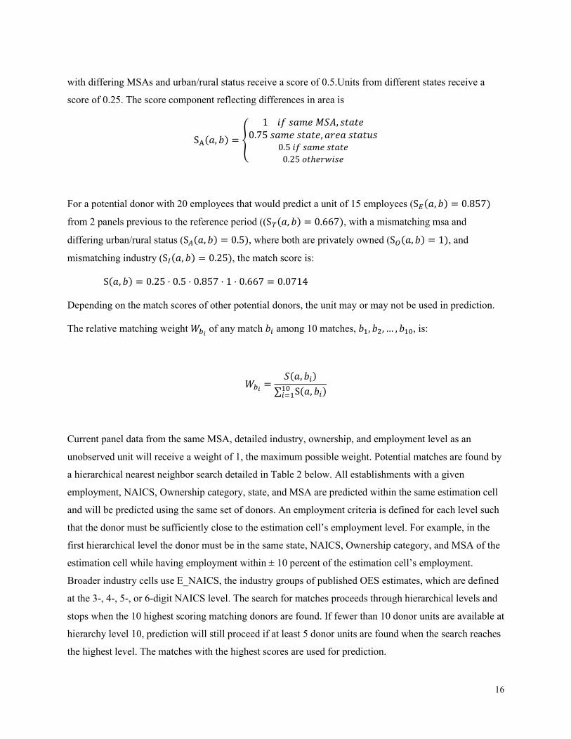
with differing MSAs and urban/rural status receive a score of 0.5.Units from different states receive a
score of 0.25. The score component reflecting differences in area is
SA(𝑎𝑎, 𝑏𝑏) = �
1 𝑖𝑖𝑖𝑖 𝑖𝑖𝑎𝑎𝑚𝑚𝑒𝑒 𝑀𝑀𝑀𝑀𝑀𝑀, 𝑖𝑖𝑖𝑖𝑎𝑎𝑖𝑖𝑒𝑒0.75 𝑖𝑖𝑎𝑎𝑚𝑚𝑒𝑒 𝑖𝑖𝑖𝑖𝑎𝑎𝑖𝑖𝑒𝑒,𝑎𝑎𝑒𝑒𝑒𝑒𝑎𝑎 𝑖𝑖𝑖𝑖𝑎𝑎𝑖𝑖𝑖𝑖𝑖𝑖
0.5 𝑖𝑖𝑖𝑖 𝑖𝑖𝑎𝑎𝑚𝑚𝑒𝑒 𝑖𝑖𝑖𝑖𝑎𝑎𝑖𝑖𝑒𝑒0.25 𝑜𝑜𝑖𝑖ℎ𝑒𝑒𝑒𝑒𝑤𝑤𝑖𝑖𝑖𝑖𝑒𝑒
For a potential donor with 20 employees that would predict a unit of 15 employees (S𝐸𝐸(𝑎𝑎, 𝑏𝑏) = 0.857)
from 2 panels previous to the reference period ((S𝑇𝑇(𝑎𝑎, 𝑏𝑏) = 0.667), with a mismatching msa and
differing urban/rural status (S𝐴𝐴(𝑎𝑎, 𝑏𝑏) = 0.5), where both are privately owned (S𝑂𝑂(𝑎𝑎, 𝑏𝑏) = 1), and
mismatching industry (S𝐼𝐼(𝑎𝑎, 𝑏𝑏) = 0.25), the match score is:
S(𝑎𝑎, 𝑏𝑏) = 0.25 ⋅ 0.5 ⋅ 0.857 ⋅ 1 ⋅ 0.667 = 0.0714
Depending on the match scores of other potential donors, the unit may or may not be used in prediction.
The relative matching weight 𝑊𝑊𝑏𝑏𝑖𝑖 of any match 𝑏𝑏𝑖𝑖 among 10 matches, 𝑏𝑏1, 𝑏𝑏2, … , 𝑏𝑏10, is:
𝑊𝑊𝑏𝑏𝑖𝑖 =𝑀𝑀(𝑎𝑎, 𝑏𝑏𝑖𝑖)
∑𝑖𝑖=110 S(𝑎𝑎, 𝑏𝑏𝑖𝑖)
Current panel data from the same MSA, detailed industry, ownership, and employment level as an
unobserved unit will receive a weight of 1, the maximum possible weight. Potential matches are found by
a hierarchical nearest neighbor search detailed in Table 2 below. All establishments with a given
employment, NAICS, Ownership category, state, and MSA are predicted within the same estimation cell
and will be predicted using the same set of donors. An employment criteria is defined for each level such
that the donor must be sufficiently close to the estimation cell’s employment level. For example, in the
first hierarchical level the donor must be in the same state, NAICS, Ownership category, and MSA of the
estimation cell while having employment within ± 10 percent of the estimation cell’s employment.
Broader industry cells use E_NAICS, the industry groups of published OES estimates, which are defined
at the 3-, 4-, 5-, or 6-digit NAICS level. The search for matches proceeds through hierarchical levels and
stops when the 10 highest scoring matching donors are found. If fewer than 10 donor units are available at
hierarchy level 10, prediction will still proceed if at least 5 donor units are found when the search reaches
the highest level. The matches with the highest scores are used for prediction.

17
Table 2: Hierarchical Levels of Donor Matches
Hierarchy Level
Characteristics that must match between the Estimation Cell and Responder (Donor)
Empl Criteria
1 State – NAICS – Ownership – MSA 10% 2 State – NAICS – Ownership – MSA 20% 3 State – NAICS – Ownership 10% 4 State – E_NAICS – Ownership 20% 5 State – NAICS – Ownership None 6 State – E_NAICS None 7 E_NAICS – Ownership 10% 8 E_NAICS – Ownership 20% 9 NAICS None 10 E_NAICS None
Table note: NAICS is 6 digit NAICS. E_NAICS is the most detailed NAICS level for which OES
publishes estimates.
Employment, staffing pattern, and wage data for the 10 closest matches are used to predict the staffing
pattern and wages of each unobserved unit. If a match differs from the unobserved unit’s employment,
occupational employment numbers will be scaled to the appropriate level. Occupational wage values are
scaled using a wage adjustment factor if a match differs from the unobserved unit in industry, ownership,
area, employment, or data collection panel. Methods for wage adjustment are discussed in the following
section. For a given unobserved unit U and set of matches 𝑏𝑏𝑖𝑖 𝑖𝑖𝑖𝑖 (𝑏𝑏1,𝑏𝑏2, … , 𝑏𝑏10), the predicted
employment E for occupation O in wage interval M will be:
𝐸𝐸𝑈𝑈𝑂𝑂𝑈𝑈 = �𝑊𝑊𝑏𝑏𝑖𝑖 ⋅𝐸𝐸𝑈𝑈𝐸𝐸𝑏𝑏𝑖𝑖
⋅ 𝐸𝐸𝑏𝑏𝑖𝑖𝑂𝑂𝑈𝑈
10
𝑖𝑖=1
where 𝐸𝐸𝑏𝑏𝑖𝑖𝑂𝑂𝑈𝑈 is the employment in wage interval M for the occupation O in establishment 𝑏𝑏𝑖𝑖, 𝐸𝐸𝑏𝑏𝑖𝑖 is the
employment for establishment 𝑏𝑏𝑖𝑖, 𝐸𝐸𝑈𝑈 is the employment of the estimation cell, and 𝑊𝑊𝑏𝑏𝑖𝑖 is the relative
matching weight of match 𝑏𝑏𝑖𝑖.The occupational wage w predicted for unit U is a weighted composite of
the occupational employment of the 10 donor units, as given by:
𝑤𝑤𝑈𝑈𝑂𝑂𝑈𝑈 = �𝑊𝑊𝑏𝑏𝑖𝑖 ⋅ AO(𝑈𝑈, 𝑏𝑏𝑖𝑖) ⋅ 𝑤𝑤𝑏𝑏𝑖𝑖𝑂𝑂𝑈𝑈 ⋅ I�𝐸𝐸𝑏𝑏𝑖𝑖𝑂𝑂𝑈𝑈 ≠ 0�/10
𝑖𝑖=1
�𝑊𝑊𝑏𝑏𝑖𝑖 ⋅ I�𝐸𝐸𝑏𝑏𝑖𝑖𝑂𝑂𝑈𝑈 ≠ 0�10
𝑖𝑖=1
18
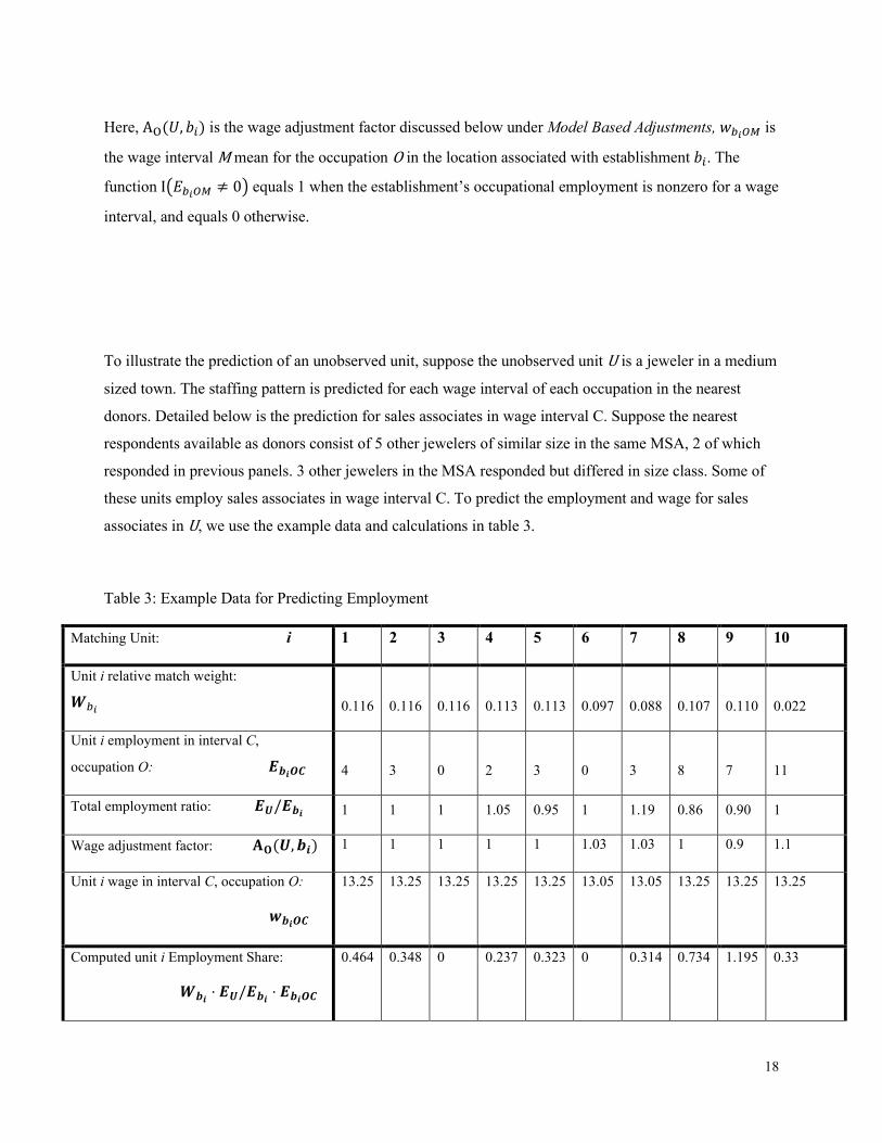
Here, AO(𝑈𝑈, 𝑏𝑏𝑖𝑖) is the wage adjustment factor discussed below under Model Based Adjustments, 𝑤𝑤𝑏𝑏𝑖𝑖𝑂𝑂𝑈𝑈 is
the wage interval M mean for the occupation O in the location associated with establishment 𝑏𝑏𝑖𝑖. The
function I�𝐸𝐸𝑏𝑏𝑖𝑖𝑂𝑂𝑈𝑈 ≠ 0� equals 1 when the establishment’s occupational employment is nonzero for a wage
interval, and equals 0 otherwise.
To illustrate the prediction of an unobserved unit, suppose the unobserved unit U is a jeweler in a medium
sized town. The staffing pattern is predicted for each wage interval of each occupation in the nearest
donors. Detailed below is the prediction for sales associates in wage interval C. Suppose the nearest
respondents available as donors consist of 5 other jewelers of similar size in the same MSA, 2 of which
responded in previous panels. 3 other jewelers in the MSA responded but differed in size class. Some of
these units employ sales associates in wage interval C. To predict the employment and wage for sales
associates in U, we use the example data and calculations in table 3.
Table 3: Example Data for Predicting Employment
Matching Unit: i 1 2 3 4 5 6 7 8 9 10
Unit i relative match weight:
𝑾𝑾𝑏𝑏𝑖𝑖 0.116 0.116 0.116 0.113 0.113 0.097 0.088 0.107 0.110 0.022
Unit i employment in interval C,
occupation O: 𝑬𝑬𝒃𝒃𝒊𝒊𝑶𝑶𝑶𝑶 4 3 0 2 3 0 3 8 7 11
Total employment ratio: 𝑬𝑬𝑼𝑼/𝑬𝑬𝒃𝒃𝒊𝒊 1 1 1 1.05 0.95 1 1.19 0.86 0.90 1
Wage adjustment factor: 𝐀𝐀𝐎𝐎(𝑼𝑼,𝒃𝒃𝒊𝒊) 1 1 1 1 1 1.03 1.03 1 0.9 1.1
Unit i wage in interval C, occupation O:
𝒘𝒘𝒃𝒃𝒊𝒊𝑶𝑶𝑶𝑶
13.25 13.25 13.25 13.25 13.25 13.05 13.05 13.25 13.25 13.25
Computed unit i Employment Share:
𝑾𝑾𝒃𝒃𝒊𝒊 ⋅ 𝑬𝑬𝑼𝑼/𝑬𝑬𝒃𝒃𝒊𝒊 ⋅ 𝑬𝑬𝒃𝒃𝒊𝒊𝑶𝑶𝑶𝑶
0.464 0.348 0 0.237 0.323 0 0.314 0.734 1.195 0.33
19
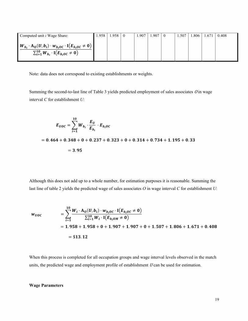
Computed unit i Wage Share:
𝑾𝑾𝒃𝒃𝒊𝒊 ⋅ 𝐀𝐀𝐎𝐎(𝑼𝑼,𝒃𝒃𝒊𝒊) ⋅ 𝒘𝒘𝒃𝒃𝒊𝒊𝑶𝑶𝑶𝑶 ⋅ 𝐈𝐈�𝑬𝑬𝒃𝒃𝒊𝒊𝑶𝑶𝑶𝑶 ≠ 𝟎𝟎�∑ 𝑾𝑾𝒃𝒃𝒊𝒊 ⋅ 𝐈𝐈�𝑬𝑬𝒃𝒃𝒊𝒊𝑶𝑶𝑶𝑶 ≠ 𝟎𝟎�𝟏𝟏𝟎𝟎𝒊𝒊=𝟏𝟏
1.958 1.958 0 1.907 1.907 0 1.507 1.806 1.671 0.408
Note: data does not correspond to existing establishments or weights.
Summing the second-to-last line of Table 3 yields predicted employment of sales associates O in wage
interval C for establishment U:
𝑬𝑬𝑼𝑼𝑶𝑶𝑶𝑶 = �𝑾𝑾𝒃𝒃𝒊𝒊 ⋅𝑬𝑬𝑼𝑼𝑬𝑬𝒃𝒃𝒊𝒊
⋅ 𝑬𝑬𝒃𝒃𝒊𝒊𝑶𝑶𝑶𝑶 𝟏𝟏𝟎𝟎
𝒊𝒊=𝟏𝟏
= 𝟎𝟎.𝟒𝟒𝟒𝟒𝟒𝟒 + 𝟎𝟎.𝟑𝟑𝟒𝟒𝟑𝟑 + 𝟎𝟎 + 𝟎𝟎.𝟐𝟐𝟑𝟑𝟐𝟐+ 𝟎𝟎.𝟑𝟑𝟐𝟐𝟑𝟑 + 𝟎𝟎 + 𝟎𝟎.𝟑𝟑𝟏𝟏𝟒𝟒 + 𝟎𝟎.𝟐𝟐𝟑𝟑𝟒𝟒 + 𝟏𝟏.𝟏𝟏𝟏𝟏𝟓𝟓 + 𝟎𝟎.𝟑𝟑𝟑𝟑
= 𝟑𝟑.𝟏𝟏𝟓𝟓
Although this does not add up to a whole number, for estimation purposes it is reasonable. Summing the
last line of table 2 yields the predicted wage of sales associates O in wage interval C for establishment U:
𝒘𝒘𝑼𝑼𝑶𝑶𝑶𝑶 = �𝑾𝑾𝒊𝒊 ⋅ 𝐀𝐀𝐎𝐎(𝑼𝑼,𝒃𝒃𝒊𝒊) ⋅ 𝒘𝒘𝒃𝒃𝒊𝒊𝑶𝑶𝑶𝑶 ⋅ 𝐈𝐈�𝑬𝑬𝒃𝒃𝒊𝒊𝑶𝑶𝑶𝑶 ≠ 𝟎𝟎�
∑ 𝑾𝑾𝒊𝒊 ⋅ 𝐈𝐈�𝑬𝑬𝒃𝒃𝒊𝒊𝑶𝑶𝑶𝑶 ≠ 𝟎𝟎�𝟏𝟏𝟎𝟎𝒊𝒊=𝟏𝟏
𝟏𝟏𝟎𝟎
𝒊𝒊=𝟏𝟏
= 𝟏𝟏.𝟏𝟏𝟓𝟓𝟑𝟑 + 𝟏𝟏.𝟏𝟏𝟓𝟓𝟑𝟑+ 𝟎𝟎 + 𝟏𝟏.𝟏𝟏𝟎𝟎𝟐𝟐 + 𝟏𝟏.𝟏𝟏𝟎𝟎𝟐𝟐 + 𝟎𝟎 + 𝟏𝟏.𝟓𝟓𝟎𝟎𝟐𝟐+ 𝟏𝟏.𝟑𝟑𝟎𝟎𝟒𝟒 + 𝟏𝟏.𝟒𝟒𝟐𝟐𝟏𝟏 + 𝟎𝟎.𝟒𝟒𝟎𝟎𝟑𝟑
= $𝟏𝟏𝟑𝟑.𝟏𝟏𝟐𝟐
When this process is completed for all occupation groups and wage interval levels observed in the match
units, the predicted wage and employment profile of establishment U can be used for estimation.
Wage Parameters

20
Wage data collection uses wage interval groups as shown in table 1 above. Using interval data to compute
mean wage estimates requires that a wage value be assigned to each employee. MB3 wage estimates use
wage interval means, which are computed using log-normal models fit to each panel of OEWS wage data
aggregated by occupation group and area group. Unobserved unit prediction further requires the
adjustment of wages for nearest neighbor unit matches to current local dollars for the unobserved unit.
For example, let’s suppose an interior design firm (NAICS 541410) in a large city contributes to the wage
predication for an industrial design firm (NAICS 541420) in a small city. Occupational wages will differ
between these firms due to both geography and industry effects. Thus, wages from the first unit must be
adjusted with these factors in mind to give a reasonable prediction of the second unit. A fixed effect
logistic regression model, fit to observed unit data, is the basis for these adjustments.
The wage interval mean model and wage adjustment model both use weighted least squares regression to
estimate model parameters. Benchmarked sample weights are used in this process, such that weighted
employment totals for the current panel will equal QCEW frame values for each industry, state, MSA,
and size subgroup. The benchmarking process is performed using the same methods applied in OEWS
design based estimates, and is detailed in the OEWS Handbook of Methods
https://www.bls.gov/opub/hom/oews/calculation.htm#preparing-data-for-estimation.
Wage Interval Mean Modeling
Wage interval means are modeled for each panel using only weighted data from that panel to represent
the population. Occupation and locality are the strongest predictors of wages and may affect substantial
differences in wage levels between establishments. To provide greater homogeneity within the data,
occupations and areas with similar wages are aggregated into groups.
Using single panel sample weights and reported employment levels within wage intervals we compute the
wage distribution for every detailed occupation (nationally across all areas) and then determine in which
interval the median wage falls. This then determines the wage occupation group for every six-digit
occupation. To be specific, we calculate occupation-specific employment in each of the twelve wage
intervals in panel p
𝐸𝐸�𝑜𝑜𝑏𝑏𝑝𝑝𝑝𝑝 = � 𝑤𝑤𝑒𝑒𝑝𝑝 × 𝐸𝐸𝑜𝑜𝑏𝑏𝑝𝑝𝑒𝑒𝑝𝑝𝑒𝑒∈𝑅𝑅𝑝𝑝

21
where 𝑅𝑅𝑝𝑝 represents the set of panel p OEWS responders, 𝑤𝑤𝑒𝑒𝑝𝑝 is the sample weight, and 𝐸𝐸𝑜𝑜𝑏𝑏𝑝𝑝𝑒𝑒𝑝𝑝 is the
reported level of employment in occupation o at establishment e in wage interval 𝑏𝑏𝑝𝑝.8 We then calculate
total occupation-specific employment
𝐸𝐸�𝑜𝑜𝑝𝑝 = � 𝐸𝐸�𝑜𝑜𝑏𝑏𝑝𝑝𝑝𝑝𝑏𝑏𝑝𝑝
and compute the relative employment shares by wage interval
�̂�𝑖𝑏𝑏𝑝𝑝|𝑜𝑜,𝑝𝑝 =𝐸𝐸�𝑜𝑜𝑏𝑏𝑝𝑝𝑝𝑝
𝐸𝐸�𝑜𝑜𝑝𝑝�
We then compute cumulative employment shares
𝜋𝜋𝑏𝑏𝑝𝑝|𝑜𝑜,𝑝𝑝 = � �̂�𝑖𝑏𝑏𝑝𝑝|𝑜𝑜,𝑝𝑝𝑏𝑏≤𝑏𝑏𝑝𝑝
The detailed occupation o is mapped into aggregate occupation O where
𝜋𝜋𝑂𝑂−1|𝑜𝑜,𝑝𝑝 < 0.5 ≤ 𝜋𝜋𝑜𝑜|𝑜𝑜,𝑝𝑝
so that an aggregate occupation is actually a wage interval.
Typically, there are either 11 or 12 aggregate occupations corresponding to the various wage intervals.
For example, the aggregate occupation group that registered nurses typically belong to is G while the
aggregate occupation group that chief executives typically belong to is L.
Similarly, we compute the wage distribution for every detailed area (across all occupations) and then
determine in which interval the median wage would fall. This then determines the aggregate area for
every detailed MSA or BOS area. To be specific, we calculate area-specific employment in each of the
twelve wage intervals 𝑏𝑏𝑝𝑝 in the current year
𝐸𝐸�𝑎𝑎𝑏𝑏𝑝𝑝𝑝𝑝 = � � 𝑤𝑤𝑒𝑒𝑝𝑝 × 𝐸𝐸𝑜𝑜𝑏𝑏𝑝𝑝𝑒𝑒𝑝𝑝𝑒𝑒∈𝑅𝑅𝑎𝑎𝑝𝑝𝑜𝑜
where 𝑅𝑅𝑎𝑎𝑝𝑝 represents the set of panel p OEWS responders in area a and wep represents the sampling
weight. We then calculate total area-specific employment
8 The wage interval is indexed by p; wage interval definitions may change across panels.

22
𝐸𝐸�𝑎𝑎𝑝𝑝 = � 𝐸𝐸�𝑎𝑎𝑏𝑏𝑝𝑝𝑝𝑝𝑏𝑏𝑝𝑝
and compute the relative employment shares by wage interval
�̂�𝑖𝑏𝑏𝑝𝑝|𝑎𝑎,𝑝𝑝 =𝐸𝐸�𝑎𝑎𝑏𝑏𝑝𝑝𝑝𝑝
𝐸𝐸�𝑎𝑎𝑝𝑝�
We then compute cumulative employment shares
𝜋𝜋𝑏𝑏𝑝𝑝|𝑎𝑎,𝑝𝑝 = � �̂�𝑖𝑏𝑏𝑝𝑝|𝑎𝑎,𝑝𝑝𝑏𝑏≤𝑏𝑏𝑝𝑝
The detailed area a is mapped into aggregate area A where
𝜋𝜋𝑀𝑀−1|𝑎𝑎,𝑝𝑝 < 0.5 ≤ 𝜋𝜋𝑀𝑀|𝑎𝑎,𝑝𝑝
so that an aggregate area is actually a wage interval.
Typically, there are only three or four aggregate areas corresponding to interval C, D, E, or F. For
example, Boston, Massachusetts typically belongs to area group E while Mobile, Alabama typically
belongs to area group C.
For every possible aggregate occupation-area, denoted as OA, we compute the single panel sample
weighted employment levels for each wage interval.
𝐸𝐸�𝑂𝑂𝑀𝑀𝑏𝑏𝑝𝑝𝑝𝑝 = � � 𝑤𝑤𝑒𝑒𝑝𝑝 × 𝐸𝐸𝑜𝑜𝑒𝑒𝑏𝑏𝑝𝑝𝑝𝑝𝑒𝑒∈𝑅𝑅𝑀𝑀𝑝𝑝𝑜𝑜∈𝑂𝑂
where 𝑅𝑅𝑀𝑀𝑝𝑝 is the panel p sample in aggregate area A. In general, there will be a limited number of
aggregate occupation-area groups, generally between 33 and 48.
A log-normal model is fit to these aggregated-occupation-by-aggregated-area cells. A maximum
likelihood estimator and the sample weighted employment sums from the current sample are used to
estimate the two parameters of the lognormal model for wage w, occupation O, and area A:
ln(𝑤𝑤𝐴𝐴𝑂𝑂) ~ N(μ𝐴𝐴𝑂𝑂,σ𝐴𝐴𝑂𝑂2 )
23
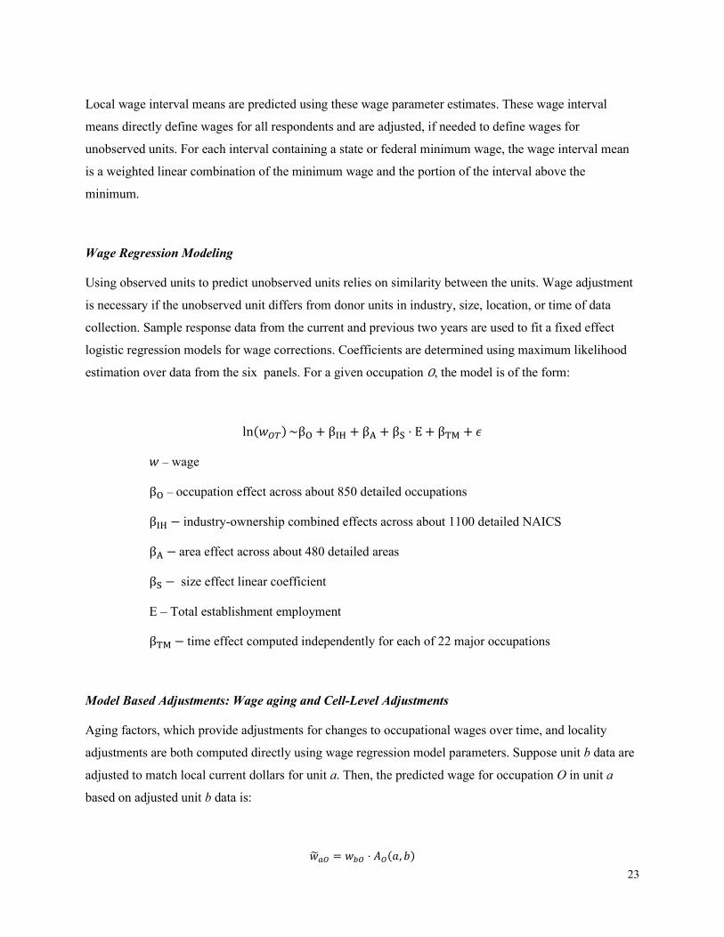
Local wage interval means are predicted using these wage parameter estimates. These wage interval
means directly define wages for all respondents and are adjusted, if needed to define wages for
unobserved units. For each interval containing a state or federal minimum wage, the wage interval mean
is a weighted linear combination of the minimum wage and the portion of the interval above the
minimum.
Wage Regression Modeling
Using observed units to predict unobserved units relies on similarity between the units. Wage adjustment
is necessary if the unobserved unit differs from donor units in industry, size, location, or time of data
collection. Sample response data from the current and previous two years are used to fit a fixed effect
logistic regression models for wage corrections. Coefficients are determined using maximum likelihood
estimation over data from the six panels. For a given occupation O, the model is of the form:
ln(𝑤𝑤𝑂𝑂𝑇𝑇) ~βO + βIH + βA + βS ⋅ E + βTM + 𝜖𝜖
𝑤𝑤 – wage
βO – occupation effect across about 850 detailed occupations
βIH − industry-ownership combined effects across about 1100 detailed NAICS
βA − area effect across about 480 detailed areas
βS − size effect linear coefficient
E – Total establishment employment
βTM − time effect computed independently for each of 22 major occupations
Model Based Adjustments: Wage aging and Cell-Level Adjustments
Aging factors, which provide adjustments for changes to occupational wages over time, and locality
adjustments are both computed directly using wage regression model parameters. Suppose unit b data are
adjusted to match local current dollars for unit a. Then, the predicted wage for occupation O in unit a
based on adjusted unit b data is:
𝑤𝑤�𝑎𝑎𝑂𝑂 = 𝑤𝑤𝑏𝑏𝑂𝑂 ⋅ 𝑀𝑀𝑂𝑂(𝑎𝑎, 𝑏𝑏)

24
Where:
𝑀𝑀𝑂𝑂(𝑎𝑎, 𝑏𝑏) = exp �βO(𝑎𝑎) + βIT(𝑎𝑎) + βA(𝑎𝑎) + βS ⋅ Ea + βMP(𝑎𝑎)βO(𝑏𝑏) + βIT(𝑏𝑏) + βA(𝑏𝑏) + βS ⋅ 𝐸𝐸𝑏𝑏 + βMP(𝑏𝑏)
�
Estimates
Occupational employment and wage estimates are computed using observed data and predicted data for
the population of about 8 million9 units. Predicted data are available for each unit of the population, so
estimates are computed using full-population expressions.
Occupational Employment Estimates
Estimates of occupational employment totals are computed by summing all employment counts of a given
occupation over the modeled population data. Estimates are made over area, industry, and ownership. For
occupation o, where unit i is any establishment in cell c, the occupational employment estimate is:
𝑋𝑋�𝑜𝑜,𝑐𝑐 = � 𝑥𝑥𝑖𝑖,𝑜𝑜𝑖𝑖∈𝑜𝑜,𝑐𝑐
Hourly wage rate estimates
Mean hourly wage is calculated as the total hourly wages for an occupation divided by its total modeled
population employment. Wage rate information is available for every individual federal employee and
some state employees. All other wage data are in wage interval ranges and are converted to local hourly
wages for each employee. These local hourly wages are predicted using adjusted estimates of local
interval means, and thus are treated as point data. Mean wage is calculated as a sum of the hourly wage
for each employees in a cell divided by the total number of employees in a cell. Employees E in a given
occupation and wage interval at a single establishment will all have the same predicted wage w. For
establishments i, wage ranges r, and occupation o in cell c, the computation is as follows:
9 Millions of units per year: 8.95 in 201902, 8.74 in 201802, 8.54 in 201702, 7.94 in 201602, 7.80 in 201502

25
𝑤𝑤�𝑐𝑐,𝑜𝑜 = ∑ ∑ 𝑥𝑥𝑖𝑖𝑖𝑖𝑜𝑜𝑖𝑖 ⋅ 𝑤𝑤𝑖𝑖𝑖𝑖𝑜𝑜𝑖𝑖∈𝑐𝑐,𝑜𝑜
∑ 𝑥𝑥𝑖𝑖𝑖𝑖𝑜𝑜𝑖𝑖∈𝑐𝑐,𝑜𝑜
Percentile wage rate estimates are computed directly from the predicted population using the empirical
distribution function with averaging, which is implemented in many statistical packages.
Annual wage rate estimates
These estimates are calculated by multiplying mean or percentile hourly wage rate estimates by a “year-
round, full time” figure of 2,080 hours (52 weeks x 40 hours) per year for most occupations. These
estimates, however, may not represent mean annual pay should the workers work more or less than 2,080
hours per year.
Alternatively, some workers are paid based on an annual basis but do not work the usual 2,080 hours per
year. For these workers, survey respondents report annual wages. Since the survey does not collect the
actual number of hours worked, hourly wage rates cannot be derived from annual wage rates with any
reasonable degree of confidence. Only annual wages are reported for some occupations.
Variance estimation
Variances for both mean wage estimates and occupational employment estimates are computed using the
“bootstrap” replication technique. Many weights may be associated with a given respondent in MB3
estimates because that respondent may be used in multiple different ways for unobserved unit prediction.
This presents problems for many approaches to computing sampling variances. However, bootstrap
sample replication is amenable to this design because the full MB3 estimation system may be applied to
each replicate sample. Studies that were performed using simulated data inform decisions on the specifics
of the bootstrapping approach used here and the number of replicates needed for estimates to converge.
The MB3 variances are computed over 300 bootstrap sample replicates. Each set of replicate estimates is
based on a subsample of the full sample, and includes model fitting as well as population prediction based
on this subsample. The subsample is drawn from the full sample using a stratified simple random sample

26
with replacement design, where the size of the subsample is equal to the size of the full sample. By
sampling with replacement, we are essentially up-weighting some sampled units by including them more
than once in the subsample while down-weighting others by not including them at all. MB3 selects six
independent subsamples, one from each of the six bi-annual OEWS panel samples. The stratification plan
is the same used for drawing the full sample, where strata are defined by state, MSAs, aggregate NAICS
industry, and ownership for schools and hospitals.
Subsampling only occurs for the non-certainty sample units. All certainty units from the full sample are
used in every replicate’s bootstrap sample. Some strata may only contain a single non-certainty unit, for
which a variance cannot be computed. These are referred to as 1-PSU strata. A collapsing algorithm
combines these 1-PSU strata with other like strata to ensure that two or more non-certainty sample units
are present in a particular stratum. The collapsing is by the hierarchy detailed in Table 4.
Table 4: Hierarchical Definitions for Collapsing 1-PSU Strata Hierarchy
Level Collapse
1 Panels*: (0,1), (2,3), and (4,5)
2 Panels*: (0, 1, 2), and (3,4,5)
3 Panels*: (0,1,2,3,4,5)
4 MSAs
5 Allocation NAICS (A_NAICS)
6 Nationally
* Panels are labeled 0 to 5, where 0 corresponds to the most recent panel
The probability of selection for resampling a given unit is proportional to that unit’s share of stratum
employment. This ensures that bootstrap sample replicates yield unbiased estimates of the full sample’s
estimates. Sampling variance estimates obtained through these methods do not use the same probabilities
used in selection of the full sample, which presents a possible source of error. Studies indicate that these
estimates are approximately unbiased and perform well in estimating sampling variance.

27
The six replicate subsamples are combined for calculating MB3 replicate estimates. Single panel sample
weights for the most recent panel are retained for computation of wage interval means and the wage
adjustment factors in each replicate. All matching, wage parameter, and estimation methods described
previously are used with each 6-panel bootstrap subsample to create occupational employment and wage
replicate estimates for every estimation domain. This process is repeated to create 300 sets of replicate
estimates. For every estimation domain in which OEWS calculates an estimate, there are occupational
employment and mean wage estimates based on the full OEWS sample as well as 300 occupational
employment and mean wage replicate estimates each based on a different bootstrap subsample. The
variance estimates for the occupational estimates based on the full sample is calculated by finding the
variability across the occupational replicate estimates. The below formula calculates the bootstrap
variance estimates:
𝑣𝑣𝐵𝐵𝐵𝐵�𝜃𝜃�𝑗𝑗,𝐷𝐷� = 1(300−1)
∑ �𝜃𝜃� 𝑗𝑗,𝐷𝐷(𝑏𝑏) − 𝜃𝜃�𝑗𝑗,D
(∗)�2
300𝑏𝑏=1
where,
𝜃𝜃�𝑗𝑗,𝐷𝐷 = occupational estimate (employment or mean wage) for occupation j, within estimation
domain D, based on full sample
𝜃𝜃�𝑗𝑗,𝐷𝐷(𝑏𝑏) = occupational replicate estimates (employment or mean wage) for occupation j, within
estimation domain D, based on the bootstrap subsample for replicate b
𝜃𝜃�𝑗𝑗,𝐷𝐷(∗) = average occupational replicate estimates (employment or mean wage) for occupation j,
within estimation domain D averaged across all 300 replicates
Special procedures
In certain circumstances, the OEWS has critical nonrespondents who could not be imputed using current
OEWS methods. OEWS employed special imputation procedures which used nonrespondents’ prior
staffing patterns and wages. The occupational employment was benchmarked to the current year and the
wage distribution was imputed using procedures very similar to the current partial imputation method.

28
In 2013, the Office of Management and Budget updated the Metropolitan Statistical Area (MSA)
definitions. The nonmetropolitan or balance-of-state areas were also updated. This resulted in the OEWS
selecting the 2016Q2 through 2014Q4 samples using the new MSA definitions, and the 2014Q2 and
2013Q4 samples using the old definitions. In order to reduce the bias introduced from using two different
MSA definitions, the sampling weights from 2014Q2 and 2013Q4 were adjusted. May 2015 was the first
time OEWS published estimates using the new MSA definitions.
Reliability of the estimates
Estimates developed from a sample will differ from the results of a census. An estimate based on a
sample survey is subject to two types of error: sampling and nonsampling error. An estimate based on a
census is subject only to nonsampling error.
Nonsampling error
This type of error is attributable to several causes, such as errors in the sampling frame; an inability to
obtain information for all establishments in the sample; differences in respondents' interpretation of a
survey question; an inability or unwillingness of the respondents to provide correct information; and
errors made in recording, coding, or processing the data. Explicit measures of the effects of nonsampling
error are not available.
Sampling error
When a sample, rather than an entire population, is surveyed, estimates differ from the true population
values that they represent. This difference, the sampling error, occurs by chance and depends on the
particular random sample used in a survey. Sampling error is characterized by the variance of the estimate
or the standard error of the estimate (square root of the variance). The relative standard error is the ratio of
the standard error to the estimate itself.
Estimates of sampling variability for occupational employment and mean wage rates are provided for all
employment and mean wage estimates to allow data users to determine if those statistics are reliable
enough for their needs. Sample estimates from a given design are said to be unbiased when an average of
the estimates from all possible samples yields the true population value. Empirical studies support that
MB3 methods provide accurate estimates of sampling variability.

29
Estimated standard errors should be taken to indicate the magnitude of sampling error only. They are not
intended to measure nonsampling error, including any biases in the data. Particular care should be
exercised in the interpretation of small estimates or of small differences between estimates when the
sampling error is relatively large or the magnitude of the bias is unknown.
Quality control measures
Several edit and quality control procedures are used to reduce nonsampling error. For example, completed
survey questionnaires are checked for data consistency. Follow-up mailings, emails, and phone calls are
sent out to nonresponding establishments to improve the survey response rate.
The OEWS survey is a federal-state cooperative effort that enables states to conduct their own surveys. A
major concern with a cooperative program such as OEWS is to accommodate the needs of BLS and other
federal agencies, as well as state-specific publication needs, with limited resources while simultaneously
standardizing survey procedures across all 50 states, the District of Columbia, and the U.S. territories.
Controlling sources of nonsampling error in this decentralized environment can be difficult. One
important computerized quality control tool used by the OEWS survey is the Survey Processing and
Management system. It was developed to provide a consistent and automated framework for survey
processing and to reduce the workload for analysts at the state, regional, and national levels.
To ensure standardized sampling methods in all areas, the sample is drawn in the national office.
Standardizing data processing activities, such as validating the sampling frame, allocating and selecting
the sample, refining mailing addresses, addressing envelopes and mailers, editing and updating
questionnaires, conducting electronic review, producing management reports, and calculating
employment estimates, have resulted in the overall standardization of the OEWS survey methodology.
This has reduced the number of errors on the data files as well as the time needed to review them.
Other quality control measures used in the OEWS survey include:
• Follow-up mail and telephone solicitations of nonrespondents, especially critical or large
nonrespondents
• Review of data during collection to verify its accuracy and reasonableness

30
• Adjustments for atypical reporting units on the data file
• Validation of unit matching and donor profiles
• Validation by comparison between MB3 research estimates and official OEWS estimates
Confidentiality
BLS has a strict confidentiality policy that ensures that the survey sample composition, lists of reporters,
and names of respondents will be kept confidential. Additionally, the policy assures respondents that
published figures will not reveal the identity of any specific respondent and will not allow the data of any
specific respondent to be inferred. The most relevant statute which governs BLS confidentiality is the
Confidential Information Protection and Statistical Efficiency Act (CIPSEA). Each published estimate is
screened to ensure that it meets these confidentiality requirements. To further protect the confidentiality
of the data, the specific screening criteria are not listed in this publication. For additional information
regarding confidentiality, please visit the BLS website at www.bls.gov/bls/confidentiality.htm.
Data presentation
Included are cross-industry data for the United States as a whole, for individual U.S. states, and for
metropolitan and nonmetropolitan areas, along with U.S. industry-specific estimates by 2-, 3-, 4-, and
some 5- and 6-digit NAICS levels. Available data include estimates of employment, annual mean wages
and relative standard errors (RSEs) for the employment and mean wage estimates.
Uses
For many years, the OEWS survey has been a major source of detailed occupational employment data for
the nation, states, and areas, and by industry at the national level. This survey provides information for
many data users, including individuals and organizations engaged in planning vocational education
programs, higher education programs, and employment and training programs. OEWS data also are used
to prepare information for career counseling, for job placement activities performed at state workforce
agencies, and for personnel planning and market research conducted by private enterprises. OEWS data
also are used by the Department of Labor’s Foreign Labor Certification (FLC) program, which sets the
rate at which workers on work visas in the United States must be paid.