survival analysis solutions to exercises - paul...

Survival analysis

Solutions to Exercises

Summer School on Modern Methods in Biostatistics and EpidemiologyCison di Valmarino, Treviso, Italy

20–25 June, 2005

http://www.bioepi.org/

Exercise solutions

1. The results are contained in the Excel file exercise1.xls and are also shown in the Stata outputbelow.

2. . ltable surv_mm csr_fail, interval(12)

Beg. Std.Interval Total Deaths Lost Survival Error [95% Conf. Int.]

-------------------------------------------------------------------------------0 12 35 7 1 0.7971 0.0685 0.6210 0.897712 24 27 1 3 0.7658 0.0726 0.5856 0.875524 36 23 5 4 0.5835 0.0901 0.3887 0.735636 48 14 2 1 0.4971 0.0953 0.3023 0.664748 60 11 0 1 0.4971 0.0953 0.3023 0.664772 84 10 0 3 0.4971 0.0953 0.3023 0.664784 96 7 0 1 0.4971 0.0953 0.3023 0.664796 108 6 1 4 0.3728 0.1292 0.1403 0.6091108 120 1 0 1 0.3728 0.1292 0.1403 0.6091

-------------------------------------------------------------------------------

. stset surv_mm, failure(status==1)

failure event: status == 1obs. time interval: (0, surv_mm]exit on or before: failure------------------------------------------------------------------------------

35 total obs.0 exclusions

------------------------------------------------------------------------------35 obs. remaining, representing16 failures in single record/single failure data

1504 total analysis time at risk, at risk from t = 0earliest observed entry t = 0

last observed exit t = 108

1

. sts list

failure _d: status == 1analysis time _t: surv_mm

Beg. Net Survivor Std.Time Total Fail Lost Function Error [95% Conf. Int.]

-------------------------------------------------------------------------------2 35 1 1 0.9714 0.0282 0.8140 0.99593 33 1 0 0.9420 0.0398 0.7873 0.98525 32 1 0 0.9126 0.0482 0.7528 0.97097 31 1 0 0.8831 0.0549 0.7178 0.95458 30 1 0 0.8537 0.0605 0.6835 0.93649 29 1 0 0.8242 0.0652 0.6499 0.917011 28 1 0 0.7948 0.0692 0.6171 0.896513 27 0 1 0.7948 0.0692 0.6171 0.896514 26 0 1 0.7948 0.0692 0.6171 0.896519 25 0 1 0.7948 0.0692 0.6171 0.896522 24 1 0 0.7617 0.0738 0.5788 0.873325 23 0 1 0.7617 0.0738 0.5788 0.873327 22 1 1 0.7271 0.0781 0.5394 0.848228 20 1 0 0.6907 0.0823 0.4989 0.821332 19 2 1 0.6180 0.0882 0.4229 0.764133 16 1 0 0.5794 0.0908 0.3837 0.732735 15 0 1 0.5794 0.0908 0.3837 0.732737 14 0 1 0.5794 0.0908 0.3837 0.732743 13 1 0 0.5348 0.0941 0.3376 0.697246 12 1 0 0.4902 0.0962 0.2944 0.660054 11 0 1 0.4902 0.0962 0.2944 0.660077 10 0 1 0.4902 0.0962 0.2944 0.660078 9 0 1 0.4902 0.0962 0.2944 0.660083 8 0 1 0.4902 0.0962 0.2944 0.660085 7 0 1 0.4902 0.0962 0.2944 0.660097 6 0 1 0.4902 0.0962 0.2944 0.6600100 5 0 1 0.4902 0.0962 0.2944 0.6600102 4 1 0 0.3677 0.1284 0.1377 0.6035103 3 0 1 0.3677 0.1284 0.1377 0.6035105 2 0 1 0.3677 0.1284 0.1377 0.6035108 1 0 1 0.3677 0.1284 0.1377 0.6035

-------------------------------------------------------------------------------

2

3533

3231

3029

2827

2320

19

1615

1211

3

0.00

0.25

0.50

0.75

1.00

0 20 40 60 80 100Time since diagnosis in months

Kaplan−Meier estimates of cause−specific survival

Figure 1: Kaplan-Meier plot of the cause-specific survivor function for sample of 35 patients diagnosedwith colon carcinoma. The number at risk at each time point are shown on the curve.

3

3. . use melanoma, clear(Skin melanoma, all stages, Finland 1975-94, follow-up to 1995)

. keep if stage == 1(2457 observations deleted)


failure event: status == 1obs. time interval: (0, surv_mm]exit on or before: failure

------------------------------------------------------------------------------5318 total obs.

0 exclusions------------------------------------------------------------------------------

5318 obs. remaining, representing1013 failures in single record/single failure data

460860.8 total analysis time at risk, at risk from t = 0earliest observed entry t = 0


. sts graph, by(year8594)

0.00

0.25

0.50

0.75

1.00

0 50 100 150 200 250analysis time

year8594 = Diagnosed 75−84 year8594 = Diagnosed 85−94

Kaplan−Meier survival estimates, by year8594

Figure 2: Skin melanoma. Kaplan-Meier plot of the cause-specific survivor function for each calendarperiod of diagnosis

(a) There seems to be a clear difference in survival between the two periods. Patients diagnosedduring 1985–94 have superior survival to those diagnosed 1975–84.

4

0.0

01.0

02.0

03.0

04

0 50 100 150 200 250analysis time

year8594 = 0 year8594 = 1

Smoothed hazard estimates, by year8594

Figure 3: Skin melanoma. Plot of the cause-specific hazard for each calendar period of diagnosis

(b) The plot shows the instantaneous cancer-specific mortality rate (the hazard) as a functionof time. It appears that mortality is highest approximately 40 months following diagnosis.Remember that all patients were classified as having localised cancer at the time of diagnosisso we would not expect mortality to be high directly following diagnosis.The plot of the hazard clearly illustrates the pattern of cancer-specific mortality as a functionof time whereas this pattern is not obvious in the plot of the survivor function.

5

4. . sts test year8594

Log-rank test for equality of survivor functions------------------------------------------------

| Eventsyear8594 | observed expected----------------+-------------------------Diagnosed 75-84 | 572 512.02Diagnosed 85-94 | 441 500.98----------------+-------------------------Total | 1013 1013.00

chi2(1) = 15.50Pr>chi2 = 0.0001

. sts test year8594, wilcoxon

Wilcoxon (Breslow) test for equality of survivor functions----------------------------------------------------------

| Events Sum ofyear8594 | observed expected ranks----------------+--------------------------------------Diagnosed 75-84 | 572 512.02 251185Diagnosed 85-94 | 441 500.98 -251185----------------+--------------------------------------Total | 1013 1013.00 0

chi2(1) = 16.74Pr>chi2 = 0.0000

There is strong evidence that survival differs between the two periods. The log-rank and theWilcoxon tests give very similar results. The Wilcoxon test gives more weight to differences insurvival in the early period of follow-up (where there are more individuals at risk) whereas the logrank test gives equal weight to all points in the follow-up. Both tests assume that, if there is adifference, a proportional hazards assumption is appropriate.

5. We start by reading the data and listing the first few observations to get an idea about the data.

. use melanoma, clear(Skin melanoma, all stages, Finland 1975-94, follow-up to 1995). list age sex stage surv_mm surv_yy osr_fail in 1/30

+---------------------------------------------------------+| age sex stage surv_mm surv_yy osr_fail ||---------------------------------------------------------|

1. | 81 Female Localised 26 2 1 |2. | 75 Female Localised 55 4 1 |3. | 78 Female Localised 177 14 1 |4. | 75 Female Unknown 29 2 1 |5. | 81 Female Unknown 57 4 1 |

|---------------------------------------------------------|

6

Now we define the data as survival time (st) data and look at the distribution of stage.


failure event: status == 1obs. time interval: (0, surv_mm]exit on or before: failure

------------------------------------------------------------7775 total obs.

0 exclusions------------------------------------------------------------



last observed exit t = 251. tab stage

Clinical |stage at |diagnosis | Freq. Percent Cum.

------------+-----------------------------------Unknown | 1,631 20.98 20.98

Localised | 5,318 68.40 89.38Regional | 350 4.50 93.88Distant | 476 6.12 100.00

------------+-----------------------------------Total | 7,775 100.00

(a) Survival depends heavily on stage. It is interesting to note that patients with stage 0 (unknown)appear to have a similar survival to patients with stage 1 (localized).

. sts graph, by(stage) xtitle(Time months)

0.00

0.25

0.50

0.75

1.00

0 50 100 150 200 250Time months

stage = Unknown stage = Localisedstage = Regional stage = Distant

Kaplan−Meier survival estimates, by stage

Figure 4: Skin melanoma. Kaplan-Meier estimates of cause-specific survival for each stage.

7

. sts graph, hazard by(stage)

0.0

1.0

2.0

3.0

4.0

5

0 50 100 150 200 250Time months

stage = 0 stage = 1stage = 2 stage = 3

Smoothed hazard estimates, by stage

Figure 5: Skin melanoma. Estimates of the hazard (cause-specific mortality rate) for each stage.

(b) . strate stage


Estimated rates and lower/upper bounds of 95% confidence intervals(7775 records included in the analysis)

+----------------------------------------------------------------+| stage D Y Rate Lower Upper ||----------------------------------------------------------------|| Unknown 274 1.2e+05 0.0022387 0.0019888 0.0025202 || Localised 1013 4.6e+05 0.0021981 0.0020668 0.0023377 || Regional 218 1.8e+04 0.0122280 0.0107079 0.0139638 || Distant 408 1.0e+04 0.0397226 0.0360493 0.0437702 |+----------------------------------------------------------------+

The time unit (defined when we stset the data) is months (since we specified surv_mm as theanalysis time). Therefore, the units of the rates shown above are events/person-month. Wecould multiply these rates by 12 to obtain estimates with units events/person-year or we canchange the default time unit by specifying the scale() option when we stset the data. Forexample,

. stset surv_mm, failure(status==1) scale(12)

. strate stagefailure _d: status == 1

analysis time _t: surv_mm/12

Estimated rates and lower/upper bounds of 95% CI(7775 records included in the analysis)+--------------------------------------------------------------+| stage D Y Rate Lower Upper ||--------------------------------------------------------------|| Unknown 274 1.0e+04 0.026865 0.023865 0.030242 || Localised 1013 3.8e+04 0.026377 0.024801 0.028052 || Regional 218 1.5e+03 0.146735 0.128494 0.167566 || Distant 408 855.9350 0.476672 0.432592 0.525243 |+--------------------------------------------------------------+

8

(c) To obtain mortality rates per 1000 person years

. strate stage, per(1000)failure _d: status == 1


Estimated rates (per 1000) and lower/upper bounds of 95% CI(7775 records included in the analysis)+----------------------------------------------------------+| stage D Y Rate Lower Upper ||----------------------------------------------------------|| Unknown 274 10.1992 26.865 23.865 30.242 || Localised 1013 38.4050 26.377 24.801 28.052 || Regional 218 1.4857 146.735 128.494 167.566 || Distant 408 0.8559 476.672 432.592 525.243 |+----------------------------------------------------------+

(d) We see that the crude mortality rate is higher for males than females, a difference which isalso reflected in the survival curves (Figure 6).

. strate sex, per(1000)failure _d: status == 1


Estimated rates (per 1000) and lower/upper bounds of 95% CI(7775 records included in the analysis)+----------------------------------------------------+| sex D Y Rate Lower Upper ||----------------------------------------------------|| Male 1074 21.8156 49.231 46.373 52.265 || Female 839 29.1302 28.802 26.917 30.818 |+----------------------------------------------------+

. sts graph, by(sex)

0.00

0.25

0.50

0.75

1.00

0 5 10 15 20analysis time

sex = Male sex = Female

Kaplan−Meier survival estimates, by sex

Figure 6: Skin melanoma (all stages). Kaplan-Meier estimates of cause-specific survival for each sex.

9

6. (a) We see that individuals with a high energy intake have a lower CHD incidence rate. Theestimated crude incidence rate ratio is 0.52.

. strate hieng, per(1000)

Estimated rates (per 1000) and lower/upper bounds of 95% confidence intervals(337 records included in the analysis)+--------------------------------------------------+| hieng D Y Rate Lower Upper ||--------------------------------------------------|| low 28 2.0594 13.5960 9.3875 19.6912 || high 18 2.5442 7.0748 4.4574 11.2291 |+--------------------------------------------------+

. display 7.0748/13.596

.52035893

(b) The IRR calculated by the Poisson regression is the same as the IRR calculated in 6(a). Atheoretical observation: If we consider the data as being cross classified solely by gender thenthe Poisson regression model with one parameter is a saturated model so the IRR estimatedfrom the model will be identical to the ‘observed’ IRR. That is, the model is a perfect fit.

. poisson chd hieng, e(y) irr

Poisson regression Number of obs = 337LR chi2(1) = 4.82Prob > chi2 = 0.0282

Log likelihood = -175.0016 Pseudo R2 = 0.0136---------------------------------------------------------------------chd | IRR Std. Err. z P>|z| [95% Conf. Interval]

------+--------------------------------------------------------------hieng | .5203602 .1572055 -2.16 0.031 .2878382 .9407184

y | (exposure)---------------------------------------------------------------------

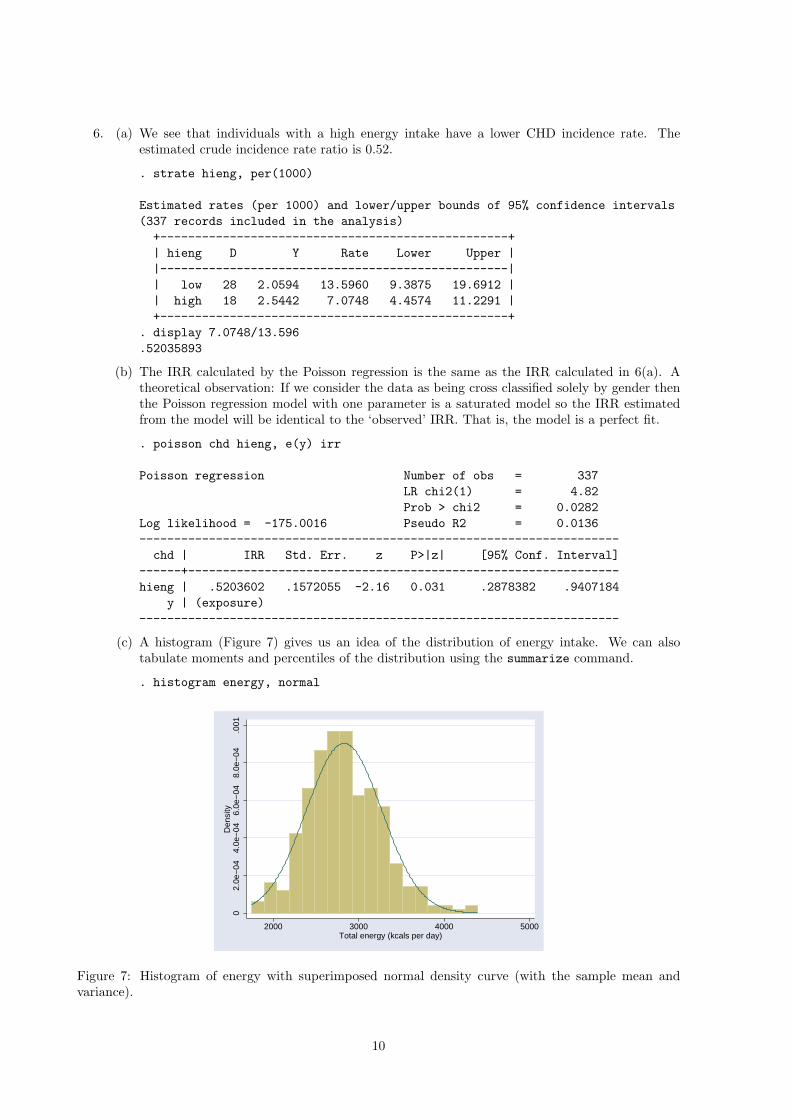
(c) A histogram (Figure 7) gives us an idea of the distribution of energy intake. We can alsotabulate moments and percentiles of the distribution using the summarize command.

. histogram energy, normal

02.

0e−

044.

0e−

046.

0e−

048.

0e−

04.0

01D

ensi

ty

2000 3000 4000 5000Total energy (kcals per day)

Figure 7: Histogram of energy with superimposed normal density curve (with the sample mean andvariance).

10

. sum energy, detail

Total energy (kcals per day)-------------------------------------------------------------

Percentiles Smallest1% 1876.13 1748.435% 2168.86 1854.0210% 2311.24 1858.8 Obs 33725% 2536.69 1876.13 Sum of Wgt. 337

50% 2802.98 Mean 2828.872Largest Std. Dev. 441.7528

75% 3109.66 4063.0290% 3366.61 4234.06 Variance 195145.595% 3595.05 4256.81 Skewness .443043499% 4063.02 4395.75 Kurtosis 3.506768

(d) . egen eng3=cut(energy), at(1500,2500,3000,4500)

. tabulate eng3

eng3 | Freq. Percent Cum.------------+-----------------------------------

1500 | 75 22.26 22.262500 | 150 44.51 66.773000 | 112 33.23 100.00

------------+-----------------------------------Total | 337 100.00

(e) We see that the CHD incidence rate decreases as the level of total energy intake increases.

. strate eng3,per(1000)

Estimated rates (per 1000) and lower/upper bounds of 95% Cis(337 records included in the analysis)+--------------------------------------------------+| eng3 D Y Rate Lower Upper ||--------------------------------------------------|| 1500 16 0.9466 16.9020 10.3547 27.5892 || 2500 22 2.0173 10.9059 7.1810 16.5629 || 3000 8 1.6398 4.8787 2.4398 9.7555 |+--------------------------------------------------+

(f) . tabulate eng3, gen(X)

eng3 | Freq. Percent Cum.------------+-----------------------------------

1500 | 75 22.26 22.262500 | 150 44.51 66.773000 | 112 33.23 100.00

------------+-----------------------------------Total | 337 100.00

11

(g) . set more off. list eng3 X1 X2 X3 if eng3==1500 in 1/100

+---------------------+| eng3 X1 X2 X3 ||---------------------|

1. | 1500 1 0 0 |2. | 1500 1 0 0 |3. | 1500 1 0 0 |4. | 1500 1 0 0 |5. | 1500 1 0 0 |

|---------------------|

. list eng3 X1 X2 X3 if eng3==2500 in 1/100+---------------------+| eng3 X1 X2 X3 ||---------------------|

76. | 2500 0 1 0 |77. | 2500 0 1 0 |78. | 2500 0 1 0 |79. | 2500 0 1 0 |80. | 2500 0 1 0 |

|---------------------|

. list eng3 X1 X2 X3 if eng3==3000 in 200/300+---------------------+| eng3 X1 X2 X3 ||---------------------|

226. | 3000 0 0 1 |227. | 3000 0 0 1 |228. | 3000 0 0 1 |229. | 3000 0 0 1 |230. | 3000 0 0 1 |

. set more on

(h) Level 1 of the categorized total energy is the reference category. The estimated rate ratiocomparing level 2 to level 1 is 0.6452 and the estimated rate ratio comparing level 3 to level 1is 0.2886.

. poisson chd X2 X3, e(y) irr


Log likelihood = -172.81043 Pseudo R2 = 0.0259------------------------------------------------------------------chd | IRR Std. Err. z P>|z| [95% Conf. Interval]----+-------------------------------------------------------------X2 | .6452416 .2120034 -1.33 0.182 .3388815 1.228561X3 | .2886479 .1249882 -2.87 0.004 .1235342 .6744495y | (exposure)

------------------------------------------------------------------

12

(i) Now use level 2 as the reference (by omitting X2 but including X1 and X3). The estimatedrate ratio comparing level 1 to level 2 is 1.5498 and the estimated rate ratio comparing level3 to level 2 is 0.4473.

. poisson chd X1 X3, e(y) irr


Log likelihood = -172.81043 Pseudo R2 = 0.0259-----------------------------------------------------------------chd | IRR Std. Err. z P>|z| [95% Conf. Interval]----+------------------------------------------------------------X1 | 1.549807 .5092114 1.33 0.182 .8139601 2.950884X3 | .4473485 .1846929 -1.95 0.051 .1991671 1.004788y | (exposure)

-----------------------------------------------------------------

(j) The estimates are identical (as we would hope) when we have Stata create indicator variablesfor us (using xi).

. xi: poisson chd i.eng3, e(y) irri.eng3 _Ieng3_1500-3000 (naturally coded; _Ieng3_1500 omitted)


Log likelihood = -172.81043 Pseudo R2 = 0.0259------------------------------------------------------------------------

chd | IRR Std. Err. z P>|z| [95% Conf. Interval]-------------+----------------------------------------------------------_Ieng3_2500 | .6452416 .2120034 -1.33 0.182 .3388815 1.228561_Ieng3_3000 | .2886479 .1249882 -2.87 0.004 .1235342 .6744495

y |(exposure)------------------------------------------------------------------------

(k) Somehow (there are many different alternatives) you’ll need to calculate the total number ofevents and the total person-time at risk and then calculate the incidence rate as events/person-time. For example,

. summarize y chd

Variable | Obs Mean Std. Dev. Min Max---------+------------------------------------------------

y | 337 13.66074 4.777274 .2874743 20.04107chd | 337 .1364985 .3438277 0 1

. display (337*0.1364985)/(337*13.66074)

.00999203

The estimated incidence rate is 0.00999 events per person-year (note that the two 337’s cancelin the calculations are are only included for completeness). We get the same answer usingstptime.

. stset dox, id(id) fail(chd) or(doe) scale(365.24)

. stptimeCohort | person-time failures rate-----------+-------------------------------------

total | 4603.7948 46 .00999176

13

7. (a) . stsplit fu, at(0(1)10) trim(0 + 1452 obs. trimmed due to lower and upper bounds)(30206 observations (episodes) created)

(b) It seems reasonable (at least to me) that melanoma-specific mortality is lower during the firstyear. These patients were classified as having localised skin melanoma at the time of diagnosis.That is, there was no evidence of metastases at the time of diagnosis although many of thepatients who died would have had undetectable metastases or micrometastases at the time ofdiagnosis. It appears that it takes at least one year for these initially undetectable metastasesto progress and cause the death of the patient.

. strate fu, per(1000) graph

failure _d: status == 1analysis time _t: surv_mm/12

id: idnote: fu>10 trimmed

Estimated rates (per 1000) and lower/upper bounds of 95% CIs(34072 records included in the analysis)+-------------------------------------------------+| fu D Y Rate Lower Upper ||-------------------------------------------------|| 0 81 5.2507 15.4266 12.4077 19.1800 || 1 233 4.8317 48.2227 42.4119 54.8297 || 2 196 4.2112 46.5429 40.4626 53.5370 || 3 139 3.6915 37.6541 31.8870 44.4641 || 4 98 3.2484 30.1685 24.7497 36.7738 ||-------------------------------------------------|| 5 77 2.8489 27.0278 21.6176 33.7920 || 6 58 2.5113 23.0953 17.8548 29.8739 || 7 29 2.1766 13.3236 9.2589 19.1729 || 8 36 1.8735 19.2154 13.8606 26.6389 || 9 14 1.5722 8.9044 5.2737 15.0349 |+-------------------------------------------------+

14

(c) The pattern is similar. The plot of the mortality rates (Figure 8) could be considered anapproximation to the ‘true’ functional form depicted in Figure 9. By estimating the rates foreach year of follow-up we are essentially approximating the curve in Figure 9 using a stepfunction. It would probably be more informative to use narrower intervals (e.g., 6-monthintervals) for the first 6 months of follow-up.

020

4060

Rat

e (p

er 1

000)

0 2 4 6 8 10fu

Figure 8: Localised melanoma. Disease-specific mortality rates as a function of time since diagnosis(annual intervals).

.01

.02

.03

.04

0 2 4 6 8 10analysis time

Smoothed hazard estimate

Figure 9: Localised melanoma. Disease-specific mortality rates as continuous function of time sincediagnosis (using a smoother).

15

(d) . xi: streg i.fu, dist(exp)i.fu _Ifu_0-10 (naturally coded; _Ifu_0 omitted)

failure _d: status == 1analysis time _t: surv_mm/12

id: idnote: fu>10 trimmed

note: _Ifu_10 dropped due to collinearity

Exponential regression -- log relative-hazard form

No. of subjects = 5318 Number of obs = 34072No. of failures = 961Time at risk = 32216.08583

LR chi2(9) = 201.23Log likelihood = -3283.9327 Prob > chi2 = 0.0000------------------------------------------------------------------------

_t | Haz. Ratio Std. Err. z P>|z| [95% Conf. Interval]-------+----------------------------------------------------------------_Ifu_1 | 3.125943 .4032046 8.84 0.000 2.427658 4.025081_Ifu_2 | 3.017055 .3985223 8.36 0.000 2.328886 3.908574_Ifu_3 | 2.440853 .3411953 6.38 0.000 1.855907 3.210162_Ifu_4 | 1.955618 .2936669 4.47 0.000 1.45701 2.624855_Ifu_5 | 1.752026 .2788568 3.52 0.000 1.282512 2.393426_Ifu_6 | 1.497108 .257516 2.35 0.019 1.068659 2.097334_Ifu_7 | .8636789 .1868991 -0.68 0.498 .5651365 1.319931_Ifu_8 | 1.2456 .2495041 1.10 0.273 .8411542 1.844511_Ifu_9 | .5772138 .1670674 -1.90 0.058 .3273158 1.017903------------------------------------------------------------------------

The pattern of the estimated mortality rate ratios mirrors the pattern we saw in the plot ofthe rates. Note that the first year of follow-up is the reference so the estimated rate ratiolabelled _Ifu_1 is the rate ratio for the second year compared to the first year.

16

(e) . xi: streg i.fu i.agegrp year8594 sex, dist(exp)i.fu _Ifu_0-10 (naturally coded; _Ifu_0 omitted)i.agegrp _Iagegrp_0-3 (naturally coded; _Iagegrp_0 omitted)


LR chi2(14) = 412.72Log likelihood = -3178.1853 Prob > chi2 = 0.0000------------------------------------------------------------------------

_t | Haz. Ratio Std. Err. z P>|z| [95% Conf. Interval]-----------+------------------------------------------------------------

_Ifu_1 | 3.198105 .4125777 9.01 0.000 2.483601 4.118164_Ifu_2 | 3.154676 .4170114 8.69 0.000 2.434647 4.08765_Ifu_3 | 2.597297 .3636721 6.82 0.000 1.973953 3.417483_Ifu_4 | 2.108206 .3174629 4.95 0.000 1.569407 2.831984_Ifu_5 | 1.908097 .3049509 4.04 0.000 1.39496 2.60999_Ifu_6 | 1.634282 .2825604 2.84 0.004 1.16455 2.293486_Ifu_7 | .9374623 .2038112 -0.30 0.766 .6122042 1.435527_Ifu_8 | 1.33826 .2701805 1.44 0.149 .9009313 1.987875_Ifu_9 | .6112851 .1779332 -1.69 0.091 .345522 1.081464

_Iagegrp_1 | 1.320821 .1242054 2.96 0.003 1.0985 1.588137_Iagegrp_2 | 1.850913 .1679404 6.79 0.000 1.549363 2.211152_Iagegrp_3 | 3.370404 .3515811 11.65 0.000 2.747196 4.13499year8594 | .7189216 .0475506 -4.99 0.000 .6315121 .8184297

sex | .5892988 .038546 -8.08 0.000 .5183923 .6699041------------------------------------------------------------------------

There is no evidence that the effect of follow-up is confounded by age, sex, and period (theestimates for fu do not change a great deal when age, sex, and period are included in themodel).

(f) . xi: streg i.fu i.agegrp year8594 i.sex i.sex*year8594, dist(exp)i.fu _Ifu_0-10 (naturally coded; _Ifu_0 omitted)i.agegrp _Iagegrp_0-3 (naturally coded; _Iagegrp_0 omitted)i.sex _Isex_1-2 (naturally coded; _Isex_1 omitted)i.sex*year8594 _IsexXyear8_# (coded as above)

Exponential regression -- log relative-hazard formNo. of subjects = 5318 Number of obs = 34072No. of failures = 961Time at risk = 32216.08583

LR chi2(15) = 412.95Log likelihood = -3178.0715 Prob > chi2 = 0.0000-------------------------------------------------------------------------

_t | Haz. Ratio Std. Err. z P>|z| [95% Conf. Interval]-------------+-----------------------------------------------------------.... [output omitted]_Iagegrp_1 | 1.31966 .1241227 2.95 0.003 1.097491 1.586804_Iagegrp_2 | 1.849583 .1678451 6.78 0.000 1.548209 2.209624_Iagegrp_3 | 3.369595 .35147 11.65 0.000 2.746578 4.133933

year8594 | .7393188 .0653467 -3.42 0.001 .6217217 .8791592_Isex_2 | .6061075 .0533638 -5.69 0.000 .5100431 .7202652

_IsexXyear~2 | .9396257 .1226729 -0.48 0.633 .7274886 1.213622-------------------------------------------------------------------------

The interaction term is not statistically significant indicating that there is no evidence thatthe effect of sex is modified by period.

17

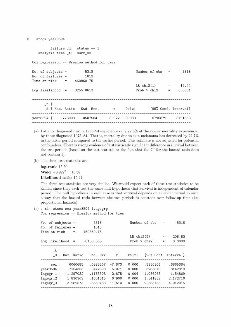
8. . stcox year8594


Cox regression -- Breslow method for ties


LR chi2(1) = 15.44Log likelihood = -8255.0613 Prob > chi2 = 0.0001

------------------------------------------------------------------------------_t |_d | Haz. Ratio Std. Err. z P>|z| [95% Conf. Interval]

---------+--------------------------------------------------------------------year8594 | .773003 .0507504 -3.922 0.000 .6796679 .8791553------------------------------------------------------------------------------

(a) Patients diagnosed during 1985–94 experience only 77.3% of the cancer mortality experiencedby those diagnosed 1975–84. That is, mortality due to skin melanoma has decreased by 22.7%in the latter period compared to the earlier period. This estimate is not adjusted for potentialconfounders. There is strong evidence of a statistically significant difference in survival betweenthe two periods (based on the test statistic or the fact that the CI for the hazard ratio doesnot contain 1).

(b) The three test statistics are

log-rank 15.50Wald −3.9222 = 15.38Likelihood ratio 15.44

The three test statistics are very similar. We would expect each of these test statistics to besimilar since they each test the same null hypothesis that survival is independent of calendarperiod. The null hypothesis in each case is that survival depends on calendar period in sucha way that the hazard ratio between the two periods is constant over follow-up time (i.e.proportional hazards).

(c) . xi: stcox sex year8594 i.agegrpCox regression -- Breslow method for ties


LR chi2(5) = 208.83Log likelihood = -8158.363 Prob > chi2 = 0.0000-----------------------------------------------------------------------

_t |_d | Haz. Ratio Std. Err. z P>|z| [95% Conf. Interval]

---------+-------------------------------------------------------------sex | .6060685 .0385507 -7.873 0.000 .5350306 .6865384

year8594 | .7154353 .0472398 -5.071 0.000 .6285878 .8142818Iagegr_1 | 1.297032 .1173508 2.875 0.004 1.086268 1.54869Iagegr_2 | 1.830303 .1601515 6.908 0.000 1.541852 2.172716Iagegr_3 | 3.282573 .3360783 11.610 0.000 2.685753 4.012015-----------------------------------------------------------------------

18

i. For patients of the same sex diagnosed in the same calendar period, those aged 60–74 atdiagnosis have an estimated 83% higher risk of death due to skin melanoma than thoseaged 0–44 at diagnosis. The difference is statistically significant.If this were an exam question the previous paragraph would be awarded full marks. Itis worth noting, however, that the analysis is adjusted for the fact that mortality maydepend on time since diagnosis (since this is the underlying time scale) and the mortalityratio between the two age groups is assumed to be the same at each point during thefollow-up (i.e., proportional hazard).

ii. No, there is no evidence of strong confounding, since the parameter estimate for periodchanges very little (from 0.77 to 0.71) when age and sex are added to the model.

iii. Age (modelled as a categorical variable with 4 levels) is highly significant in the model.. test _Iagegrp_1 _Iagegrp_2 _Iagegrp_3

chi2( 3) = 153.65Prob > chi2 = 0.0000

(d) Age (modelled as a categorical variable with 4 levels) is highly significant in the model. TheWald test is an approximation to the LR test and we would expect the two to be similar (whichthey are).

. lrtest Alikelihood-ratio test LR chi2(3) = 142.50(Assumption: . nested in A) Prob > chi2 = 0.0000

(e) i. Both models adjust for the same factors. When fitting the Poisson regression model wesplit time since diagnosis into annual intervals and explicitly estimated the effect of thisfactor in the model. The Cox model does not estimate the effect of ‘time’ but the otherestimates are adjusted for ‘time’.

ii. Since the two models are conceptually similar we would expect the parameter estimatesto be similar, which they are.

_t | Haz. Ratio Std. Err. z P>|z| [95% CI]-------------+----------------------------------------------------------Cox regression

sex | .6060685 .0385507 -7.87 0.000 .5350306 .6865384year8594 | .7154353 .0472398 -5.07 0.000 .6285878 .8142818

_Iagegrp_1 | 1.297032 .1173508 2.87 0.004 1.086268 1.54869_Iagegrp_2 | 1.830303 .1601515 6.91 0.000 1.541852 2.172716_Iagegrp_3 | 3.282573 .3360783 11.61 0.000 2.685753 4.012015

Poisson regressionsex | .5892988 .038546 -8.08 0.000 .5183923 .6699041

year8594 | .7189216 .0475506 -4.99 0.000 .6315121 .8184297_Iagegrp_1 | 1.320821 .1242054 2.96 0.003 1.0985 1.588137_Iagegrp_2 | 1.850913 .1679404 6.79 0.000 1.549363 2.211152_Iagegrp_3 | 3.370404 .3515811 11.65 0.000 2.747196 4.13499

iii. Yes, both models assume ‘proportional hazards’. The proportional hazards assumptionimplies that the risk ratios for sex, period, and age are constant across all levels of follow-up time. In other words, the assumption is that there is no effect modification by follow-uptime. This assumption is implicit in Poisson regression (as it is in logistic regression) whereit is assumed that estimated risk ratios are constant across all combination of the othercovariates. We can, of course, relax this assumption by fitting interaction terms.

19

9. . stphplot, by(year8594)

02

46

8−

ln[−

ln(S

urvi

val P

roba

bilit

y)]

−4 −2 0 2 4 6ln(analysis time)

year8594 = Diagnosed 75−84 year8594 = Diagnosed 85−94

Figure 10: Localised skin melanoma. Plot of the log cumulative hazard function for each calendar periodof diagnosis. Each plot symbol represents an event time.

. sts graph, hazard by(year8594)

0.0

01.0

02.0

03.0

04

0 50 100 150 200 250analysis time

year8594 = 0 year8594 = 1

Smoothed hazard estimates, by year8594

Figure 11: Localised skin melanoma. Plot of the estimated hazard function for each calendar period ofdiagnosis.

(a) We know that patients diagnosed during 1984–95 have superior survival. Consequently, theyhave a lower cumulative hazard, a lower log cumulative hazard, and therefore a higher negativelog cumulative hazard. The difference between the two curves is similar over time, except forone point where the curves cross. As such, there is no reason to reject an assumption ofproportional hazards.

20

We should not pay too much attention to the curves for values up to 2 on the x axis. Notingthat exp(2) = 7.4 we see that the curves between 0 and 2 on the x axis are based on only 7data points. We should give more weight to differences where we have more data.

(b) The log rank test assumes that any difference in survival between the groups takes the formof proportional hazards. As such, the log rank test may fail to detect a difference in survivalif the difference does not take the form of proportional hazards.

(c) A rough estimate of the difference between the curves is 0.2, which is an estimate of the loghazard ratio. An estimate of the hazard ratio is therefore exp(−0.2) = 0.82.

(d) The estimated hazard ratio from the Cox model is 0.77 which is similar (as it should be) tothe estimate made by looking at the difference in the plots of the log cumulative hazard.

(e) It seems that there is evidence of non-proportional hazards, particularly for age and sex.

. stphtest, detail

Test of proportional hazards assumption---------------------------------------------

| rho chi2 df Prob>chi2------------+--------------------------------sex | 0.07535 5.65 1 0.0175year8594 | 0.03335 1.12 1 0.2896_Iagegrp_1 | -0.05293 2.84 1 0.0919_Iagegrp_2 | -0.07392 5.49 1 0.0192_Iagegrp_3 | -0.11356 12.40 1 0.0004------------+--------------------------------global test | 17.94 5 0.0030---------------------------------------------

(f) The differences in survival by age are most apparent early in the follow-up.

. stphplot, by(agegrp)

02

46

8−

ln[−

ln(S

urvi

val P

roba

bilit

y)]

−4 −2 0 2 4 6ln(analysis time)

agegrp = 0−44 agegrp = 45−59agegrp = 60−74 agegrp = 75+

Figure 12: Localised skin melanoma. Plot of the log cumulative hazard function for each age group. Eachplot symbol represents an event time.

21

. sts graph, hazard by(agegrp)

0.0

02.0

04.0

06.0

08

0 50 100 150 200 250analysis time

agegrp = 0 agegrp = 1agegrp = 2 agegrp = 3

Smoothed hazard estimates, by agegrp

Figure 13: Localised skin melanoma. Plot of the estimated hazard function for each age group.

−5

05

10sc

aled

Sch

oenf

eld

− _

Iage

grp_

3

0 50 100 150 200 250Time

bandwidth = .8

Test of PH Assumption

Figure 14: Localised skin melanoma. Plot of the scaled Schoenfeld residuals for age3.

If the proportional hazards assumption is appropriate then we should see parallel lines inFigure 12. This doesn’t look too bad, apart from the line for the oldest age group beingsomewhat lower than the others in the early period. Note that these curves are not based onthe estimated Cox model (i.e., they are unadjusted).It’s difficult to assess the PH hypothesis from Figure 13 although this figure does give us a goodidea of the shape of the underlying hazards. Do we really expect hazards to be proportionalover the entire 200 month follow-up period when the magnitude of mortality varies greatlyover this interval? Note that these curves are not based on the estimated Cox model (i.e., theyare unadjusted).

22

We saw evidence of non-proportional hazards by age, particularly in the eldest age group. Thesmooth line in Figure 14 shows the estimated hazard ratio as a function of time. We see thatthe estimated hazard ratio is highest immediately following diagnosis, decreases over the first100 months and is then relatively constant.

(g) . stcox sex year8594 _Iagegrp_1 _Iagegrp_2 _Iagegrp_3,tvc( _Iagegrp_1 _Iagegrp_2 _Iagegrp_3) texp(_t>=24)

------------------------------------------------------------------------------_t | Haz. Ratio Std. Err. z P>|z| [95% Conf. Interval]

-------------+----------------------------------------------------------------rh |

sex | .6081152 .0386691 -7.82 0.000 .5368579 .6888305year8594 | .7137211 .0471632 -5.10 0.000 .6270189 .8124123

_Iagegrp_1 | 1.702949 .3343537 2.71 0.007 1.158987 2.502217_Iagegrp_2 | 2.461019 .4612078 4.81 0.000 1.704494 3.553322_Iagegrp_3 | 5.390195 1.033536 8.79 0.000 3.701621 7.849048

-------------+----------------------------------------------------------------t |_Iagegrp_1 | .7081921 .1567346 -1.56 0.119 .4589508 1.092788_Iagegrp_2 | .6847885 .145389 -1.78 0.075 .4516853 1.03819_Iagegrp_3 | .4801757 .1107029 -3.18 0.001 .3056036 .7544699

------------------------------------------------------------------------------

The hazard ratios for age in the top panel are for the first two years subsequent to diagnosis.To obtain the hazard ratios for the period two years or more following diagnosis we multiplythe hazard ratios in the top and bottom panel. That is, during the first two years followingdiagnosis patients aged 75 years or more at diagnosis have 5.4 times higher cancer-specificmortality than patients aged 0–44 at diagnosis. During the period two years or more followingdiagnosis the corresponding hazard ratio is 5.39 × 0.48 = 2.59. Note that simply cutting thefollow-up at 2 years probably does adequately capture the manner in which the effect of agevaries as a function of time since diagnosis.

23

(h) The approach is to split the data at 24 months since diagnosis and fit a model with aninteraction between follow-up and age. We first need to create an ID variable.

. use melanoma, clear

. keep if stage == 1

. gen id=_n

. stset surv_mm, failure(status==1) id(id)

. list id surv_mm _st _d _t0 _t if id < 5

+-------------------------------------+

| id surv_mm _st _d _t0 _t |

|-------------------------------------|

1. | 1 26 1 0 0 26 |

2. | 2 55 1 0 0 55 |

3. | 3 177 1 0 0 177 |

4. | 4 19 1 1 0 19 |

+-------------------------------------+

. stsplit fu, at(24)

. list id surv_mm _st _d _t0 _t fu if id < 5, sepby(id)

+------------------------------------------+

| id surv_mm _st _d _t0 _t fu |

|------------------------------------------|

1. | 1 24 1 0 0 24 0 |

2. | 1 26 1 0 24 26 24 |

|------------------------------------------|

3. | 2 24 1 0 0 24 0 |

4. | 2 55 1 0 24 55 24 |

|------------------------------------------|

5. | 3 24 1 0 0 24 0 |

6. | 3 177 1 0 24 177 24 |

|------------------------------------------|

7. | 4 19 1 1 0 19 0 |

+------------------------------------------+

. xi: streg sex year8594 i.agegrp*i.fu, dist(exp)

No. of subjects = 5318 Number of obs = 9809

No. of failures = 1013

Time at risk = 460860.03 LR chi2(9) = 246.18

Log likelihood = -3490.6961 Prob > chi2 = 0.0000

------------------------------------------------------------------------------

_t | Haz. Ratio Std. Err. z P>|z| [95% Conf. Interval]

-------------+----------------------------------------------------------------

sex | .5931472 .0377298 -8.21 0.000 .5236221 .6719037

year8594 | .9323015 .0612735 -1.07 0.286 .8196208 1.060473

_Iagegrp_1 | 1.594928 .304503 2.45 0.014 1.097059 2.318741

_Iagegrp_2 | 2.35879 .427177 4.74 0.000 1.654005 3.363891

_Iagegrp_3 | 4.859066 .9021761 8.51 0.000 3.376847 6.991884

_Ifu_24 | 1.133585 .1938742 0.73 0.463 .8107283 1.585014

_IageXfu_1~4 | .7914908 .1716243 -1.08 0.281 .5174568 1.210648

_IageXfu_2~4 | .7886481 .1633875 -1.15 0.252 .525456 1.183669

_IageXfu_3~4 | .6953743 .1572626 -1.61 0.108 .4463905 1.083234

------------------------------------------------------------------------------

We have estimated an additional parameter compared to the Cox model (the hazard ratiobetween the two calendar periods _Ifu_24). The parameters _Iagegrp_1–_Iagegrp_3 givethe effect of age during the first 24 months of follow-up and are similar to the estimates fromthe Cox model. They are not identical since Poisson regression makes the assumption that thehazards are constant within this interval whereas the Cox model does not. There are greaterdifferences in the estimates of the interaction effects since the assumption that the hazards areconstant during the second interval is less sound (than the assumption that the hazards areconstant during the first interval).

24

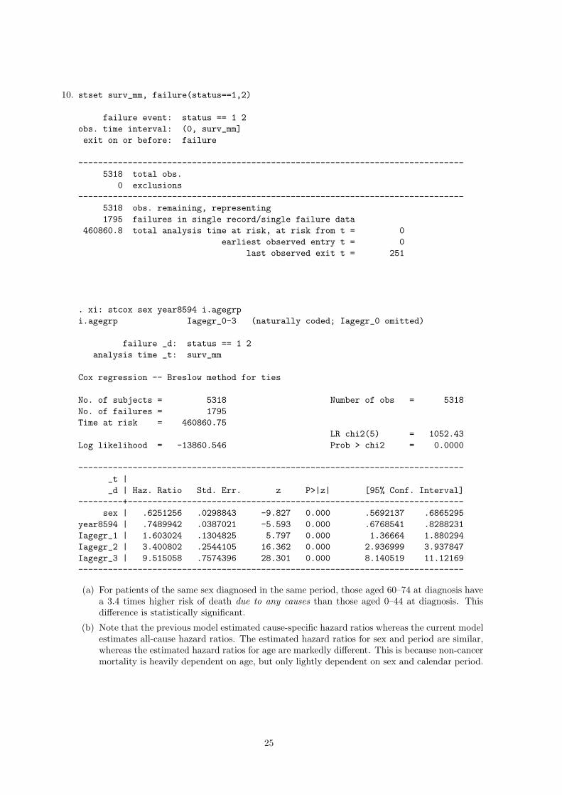
10. stset surv_mm, failure(status==1,2)

failure event: status == 1 2obs. time interval: (0, surv_mm]exit on or before: failure

------------------------------------------------------------------------------5318 total obs.

0 exclusions------------------------------------------------------------------------------




. xi: stcox sex year8594 i.agegrpi.agegrp Iagegr_0-3 (naturally coded; Iagegr_0 omitted)

failure _d: status == 1 2analysis time _t: surv_mm




------------------------------------------------------------------------------_t |_d | Haz. Ratio Std. Err. z P>|z| [95% Conf. Interval]

---------+--------------------------------------------------------------------sex | .6251256 .0298843 -9.827 0.000 .5692137 .6865295

year8594 | .7489942 .0387021 -5.593 0.000 .6768541 .8288231Iagegr_1 | 1.603024 .1304825 5.797 0.000 1.36664 1.880294Iagegr_2 | 3.400802 .2544105 16.362 0.000 2.936999 3.937847Iagegr_3 | 9.515058 .7574396 28.301 0.000 8.140519 11.12169------------------------------------------------------------------------------

(a) For patients of the same sex diagnosed in the same period, those aged 60–74 at diagnosis havea 3.4 times higher risk of death due to any causes than those aged 0–44 at diagnosis. Thisdifference is statistically significant.

(b) Note that the previous model estimated cause-specific hazard ratios whereas the current modelestimates all-cause hazard ratios. The estimated hazard ratios for sex and period are similar,whereas the estimated hazard ratios for age are markedly different. This is because non-cancermortality is heavily dependent on age, but only lightly dependent on sex and calendar period.

25

11. (a) . stcox sex



LR chi2(1) = 103.25Log likelihood = -16342.555 Prob > chi2 = 0.0000---------------------------------------------------------------------_t | Haz. Ratio Std. Err. z P>|z| [95% Conf. Interval]----+----------------------------------------------------------------sex | .6273066 .0289338 -10.11 0.000 .573085 .6866581---------------------------------------------------------------------

We see, without adjusting for potential confounders, that females have a 38% lower mortalitythan males.

(b) . xi: stcox sex year8594 i.agegrp i.subsite i.stagei.agegrp _Iagegrp_0-3 (naturally coded; _Iagegrp_0 omitted)i.subsite _Isubsite_1-4 (naturally coded; _Isubsite_1 omitted)i.stage _Istage_0-3 (naturally coded; _Istage_0 omitted)



LR chi2(11) = 1835.82Log likelihood = -15476.269 Prob > chi2 = 0.0000-------------------------------------------------------------------------

_t | Haz. Ratio Std. Err. z P>|z| [95% Conf. Interval]------------+------------------------------------------------------------

sex | .7490676 .036445 -5.94 0.000 .6809368 .8240153year8594 | .7867739 .0376881 -5.01 0.000 .7162681 .8642199

_Iagegrp_1 | 1.268542 .0855596 3.53 0.000 1.111459 1.447824_Iagegrp_2 | 1.730767 .1126805 8.43 0.000 1.523427 1.966326_Iagegrp_3 | 2.785848 .2128337 13.41 0.000 2.398431 3.235845_Isubsite_2 | 1.393153 .0984179 4.69 0.000 1.213016 1.600041_Isubsite_3 | 1.032021 .0767263 0.42 0.672 .8920829 1.19391_Isubsite_4 | 1.305318 .133562 2.60 0.009 1.06812 1.59519_Istage_1 | 1.038328 .0713262 0.55 0.584 .9075334 1.187972_Istage_2 | 4.771515 .4363494 17.09 0.000 3.988549 5.70818_Istage_3 | 13.48664 1.097917 31.96 0.000 11.49766 15.8197

-------------------------------------------------------------------------

After adjusting for a range of potential confounders we see that the estimated difference incancer-specific mortality between males and females has decreased slightly but there is stillquite a large difference.

26

(c) Let’s first estimate the effect of gender for each age group without adjusting for confounders.. gen fem0=(sex==2)*(agegrp==0)

. gen fem1=(sex==2)*(agegrp==1)



. xi: stcox i.agegrp fem0 fem1 fem2 fem3





------------------------------------------------------------------------------


-------------+----------------------------------------------------------------

_Iagegrp_1 | 1.197101 .1017692 2.12 0.034 1.013369 1.414145

_Iagegrp_2 | 1.497299 .1267028 4.77 0.000 1.268466 1.767412

_Iagegrp_3 | 2.322161 .2401309 8.15 0.000 1.896142 2.843895

fem0 | .4578165 .0478157 -7.48 0.000 .3730692 .5618151

fem1 | .5526258 .0504729 -6.49 0.000 .4620494 .660958

fem2 | .7132982 .0565997 -4.26 0.000 .6105607 .833323

fem3 | .6750958 .0713516 -3.72 0.000 .5487834 .8304813

------------------------------------------------------------------------------

. test fem0=fem1=fem2=fem3

chi2( 3) = 13.50 Prob > chi2 = 0.0037

We see that there is some evidence that the survival advantage experienced by females dependson age. The hazard ratio for males/females in the youngest age group is 0.46, while in thehighest age group the hazard ratio is 0.68. There is evidence that the hazard ratios for genderdiffer across the age groups (p=0.0037). However, after adjusting for stage, subsite, and periodthere is no longer evidence of an interaction. See the following.

. xi: stcox i.agegrp year8594 i.subsite i.stage fem0 fem1 fem2 fem3





------------------------------------------------------------------------------


-------------+----------------------------------------------------------------

_Iagegrp_1 | 1.188947 .1014449 2.03 0.043 1.005855 1.405367

_Iagegrp_2 | 1.5508 .1318113 5.16 0.000 1.312827 1.831911

_Iagegrp_3 | 2.485421 .2605605 8.68 0.000 2.023782 3.052363

year8594 | .7868595 .0376845 -5.01 0.000 .7163599 .8642973

_Isubsite_2 | 1.401988 .0992064 4.78 0.000 1.220428 1.610558

_Isubsite_3 | 1.039415 .0773326 0.52 0.603 .8983792 1.202593

_Isubsite_4 | 1.315538 .1349198 2.67 0.007 1.075983 1.608428

_Istage_1 | 1.036942 .0712433 0.53 0.598 .9063011 1.186414

_Istage_2 | 4.702828 .4312718 16.88 0.000 3.929161 5.628833

_Istage_3 | 13.38869 1.091144 31.83 0.000 11.41215 15.70757

fem0 | .6251314 .0662091 -4.44 0.000 .5079472 .7693502

fem1 | .7300673 .0678894 -3.38 0.001 .608428 .8760252

fem2 | .8120201 .0653462 -2.59 0.010 .6935337 .9507494

fem3 | .8068979 .086154 -2.01 0.044 .654537 .9947249

------------------------------------------------------------------------------

. test fem0=fem1=fem2=fem3

chi2( 3) = 4.56 Prob > chi2 = 0.2067

That is, there is not strong evidence in support of the hypothesis (although some may considerthat there is weak evidence).

(d)

27

12. (a). poisson chd hieng, e(y) irr


Log likelihood = -175.0016 Pseudo R2 = 0.0136-----------------------------------------------------------------------chd | IRR Std. Err. z P>|z| [95% Conf. Interval]

------+----------------------------------------------------------------hieng | .5203602 .1572055 -2.16 0.031 .2878382 .9407184

y | (exposure)-----------------------------------------------------------------------

. /* Cox model with time in study as the scale */

. stset dox, id(id) fail(chd) origin(doe) scale(365.25)

. stcox hieng

Cox regression -- no ties



_t | Haz. Ratio Std. Err. z P>|z| [95% Conf. Interval]------+----------------------------------------------------------------hieng | .5233587 .15814 -2.14 0.032 .2894658 .9462409-----------------------------------------------------------------------

These two models are conceptually different since the Cox model adjusts for ‘time’ even thoughthis is not explicit in the stcox command. In this example, ‘time’ refers to ‘time on study’(time since entry) which we do not expect to be a strong confounder. That is, we would expectthe estimates of the effect of high energy to be similar for the two models, which they are.

(b) If we use a different timescale then this amounts to adjusting for a different factor. As such,we would not expect the estimates to be identical. Attained age, unlike time since entry, isexpected to be a confounder but we see that it is not a strong confounder.

. /* Cox model with attained age as the scale */

. stset dox, id(id) fail(chd) origin(dob) entry(doe) scale(365.25)

. stcox hieng




------------------------------------------------------------------------------_t | Haz. Ratio Std. Err. z P>|z| [95% Conf. Interval]

-------------+----------------------------------------------------------------hieng | .5426351 .1643032 -2.02 0.043 .2997606 .9822933

------------------------------------------------------------------------------

28

13. (a) . use brv, clear

. list id sex doe dosp dox fail if couple==3+-----------------------------------------------------+| id sex doe dosp dox fail ||-----------------------------------------------------|

168. | 60 1 20jan1981 31dec1981 03aug1981 1 |384. | 63 2 20jan1981 03aug1981 31dec1981 1 |

+-----------------------------------------------------+

. list id sex doe dosp dox fail if couple==4+------------------------------------------------------+| id sex doe dosp dox fail ||------------------------------------------------------|

12. | 156 1 20jan1981 23nov1988 01jan1991 0 |300. | 220 2 20jan1981 01jan2000 23nov1988 1 |

+------------------------------------------------------+

. list id sex doe dosp dox fail if couple==19+-------------------------------------------------------+| id sex doe dosp dox fail ||-------------------------------------------------------|

167. | 2122 1 06may1981 01jan2000 01jan1991 0 |298. | 2128 2 06may1981 01jan2000 01jan1991 0 |

+-------------------------------------------------------+

(b) . stset dox, fail(fail) origin(dob) entry(doe) scale(365.25) id(id) noshow

id: idfailure event: fail != 0 & fail < .

obs. time interval: (dox[_n-1], dox]enter on or after: time doeexit on or before: failure

t for analysis: (time-origin)/365.25origin: time dob

------------------------------------------------------------------------------399 total obs.0 exclusions

------------------------------------------------------------------------------399 obs. remaining, representing399 subjects278 failures in single failure-per-subject data

2435.641 total analysis time at risk, at risk from t = 0earliest observed entry t = 75.13758

last observed exit t = 96.50376

. strate sex, per(1000)

Estimated rates (per 1000) and lower/upper bounds of 95% confidence intervals(399 records included in the analysis)+--------------------------------------------------+| sex D Y Rate Lower Upper ||--------------------------------------------------|| 1 181 1.3405 135.026 116.721 156.202 || 2 97 1.0952 88.572 72.589 108.074 |+--------------------------------------------------+

29

i. The timescale is attained age, which would seem to be a reasonable choice.ii. Males have the higher mortality which is to be expected.iii. Age could potentially be a confounder.

. tabstat _t0, by(sex)

Summary for variables: _t0by categories of: sex (1=M, 2=F)

sex | mean---------+----------

1 | 79.069362 | 78.6578

---------+----------Total | 78.90123

--------------------

Males are slightly older at diagnosis (although we haven’t studied pairwise differences).

. streg sex, dist(exp) nologExponential regression -- log relative-hazard formNo. of subjects = 399 Number of obs = 399No. of failures = 278Time at risk = 2435.641342

LR chi2(1) = 11.64Log likelihood = 355.79411 Prob > chi2 = 0.0006---------------------------------------------------------------------_t | Haz. Ratio Std. Err. z P>|z| [95% Conf. Interval]----+----------------------------------------------------------------sex | .6559621 .0825422 -3.35 0.001 .5125885 .839438---------------------------------------------------------------------

30

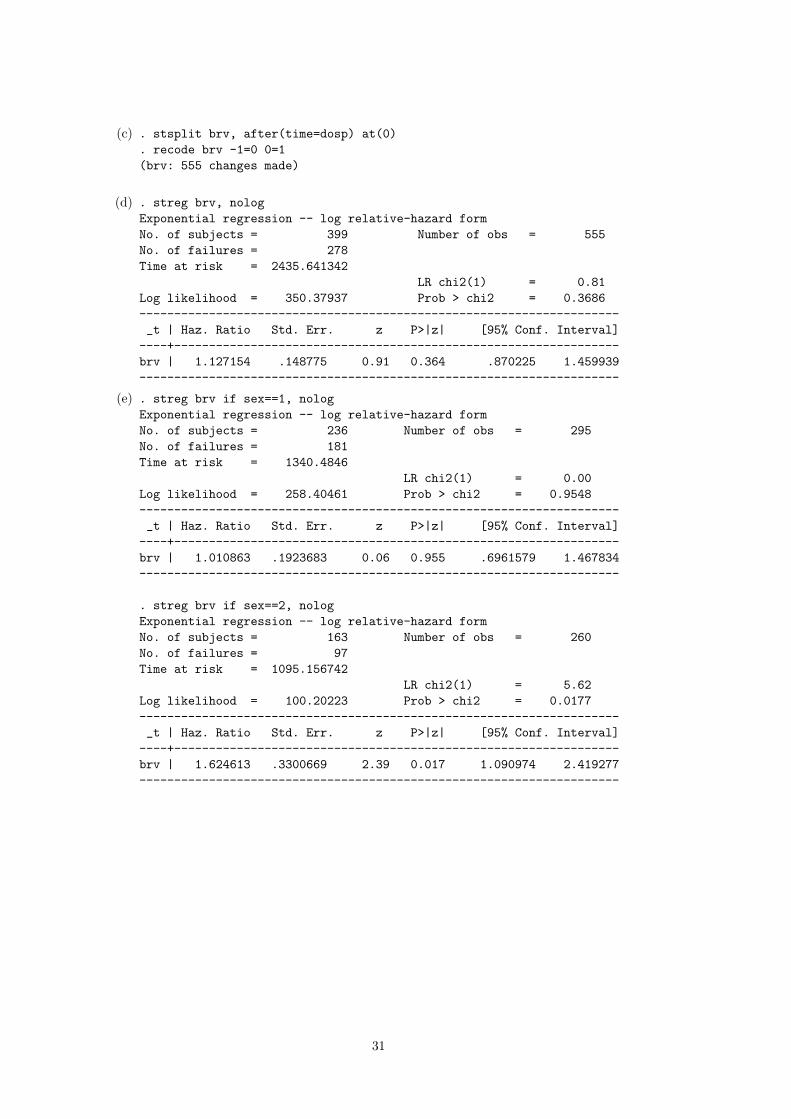
(c) . stsplit brv, after(time=dosp) at(0). recode brv -1=0 0=1(brv: 555 changes made)

(d) . streg brv, nologExponential regression -- log relative-hazard formNo. of subjects = 399 Number of obs = 555No. of failures = 278Time at risk = 2435.641342

LR chi2(1) = 0.81Log likelihood = 350.37937 Prob > chi2 = 0.3686---------------------------------------------------------------------_t | Haz. Ratio Std. Err. z P>|z| [95% Conf. Interval]----+----------------------------------------------------------------brv | 1.127154 .148775 0.91 0.364 .870225 1.459939---------------------------------------------------------------------

(e) . streg brv if sex==1, nologExponential regression -- log relative-hazard formNo. of subjects = 236 Number of obs = 295No. of failures = 181Time at risk = 1340.4846

LR chi2(1) = 0.00Log likelihood = 258.40461 Prob > chi2 = 0.9548---------------------------------------------------------------------_t | Haz. Ratio Std. Err. z P>|z| [95% Conf. Interval]----+----------------------------------------------------------------brv | 1.010863 .1923683 0.06 0.955 .6961579 1.467834---------------------------------------------------------------------

. streg brv if sex==2, nologExponential regression -- log relative-hazard formNo. of subjects = 163 Number of obs = 260No. of failures = 97Time at risk = 1095.156742

LR chi2(1) = 5.62Log likelihood = 100.20223 Prob > chi2 = 0.0177---------------------------------------------------------------------_t | Haz. Ratio Std. Err. z P>|z| [95% Conf. Interval]----+----------------------------------------------------------------brv | 1.624613 .3300669 2.39 0.017 1.090974 2.419277---------------------------------------------------------------------

31

Now we create indicator variables (brv_m and brv_f) to allow us to estimate the effect ofbereavement separately for each sex.

. gen brv_m=brv*(sex==1)

. gen brv_f=brv*(sex==2)

. streg sex brv_m brv_f, nolog

Exponential regression -- log relative-hazard form


LR chi2(3) = 17.26Log likelihood = 358.60684 Prob > chi2 = 0.0006

-----------------------------------------------------------------------_t | Haz. Ratio Std. Err. z P>|z| [95% Conf. Interval]

------+----------------------------------------------------------------sex | .5348431 .087562 -3.82 0.000 .3880357 .737193

brv_m | 1.010863 .1923683 0.06 0.955 .6961579 1.467834brv_f | 1.624613 .3300669 2.39 0.017 1.090974 2.419277-----------------------------------------------------------------------

(f) . /* Split by attained age */. stsplit age, at(70(5)100)(481 observations (episodes) created)

. strate ageEstimated rates and lower/upper bounds of 95% confidence intervals(1036 records included in the analysis)+-------------------------------------------------------+| age D Y Rate Lower Upper ||-------------------------------------------------------|| 75 45 704.1123 0.063910 0.047718 0.085597 || 80 123 1.2e+03 0.103831 0.087012 0.123902 || 85 95 489.6099 0.194032 0.158687 0.237249 || 90 12 55.0205 0.218100 0.123861 0.384041 || 95 3 2.2868 1.311883 0.423110 4.067583 |+-------------------------------------------------------+

32

. /* Poisson regression: effect of bereavementcontrolled for attained age */

. xi: streg brv i.age, nolog


LR chi2(5) = 56.78Log likelihood = 378.36458 Prob > chi2 = 0.0000-----------------------------------------------------------------------

_t | Haz. Ratio Std. Err. z P>|z| [95% Conf. Interval]---------+-------------------------------------------------------------

brv | .8591401 .1178292 -1.11 0.268 .6566342 1.124099_Iage_80 | 1.667713 .2929561 2.91 0.004 1.181942 2.353132_Iage_85 | 3.203792 .5989022 6.23 0.000 2.22098 4.621511_Iage_90 | 3.621248 1.191405 3.91 0.000 1.900245 6.90092_Iage_95 | 21.10446 12.59434 5.11 0.000 6.552538 67.97337-----------------------------------------------------------------------

. /* Poisson regression: effect of bereavementcontrolled for attained age and sex */

. xi: streg sex brv i.age, nologLR chi2(6) = 71.55

Log likelihood = 385.75207 Prob > chi2 = 0.0000----------------------------------------------------------------------

_t | Haz. Ratio Std. Err. z P>|z| [95% Conf. Interval]---------+------------------------------------------------------------

sex | .6113709 .0798235 -3.77 0.000 .4733342 .7896627brv | .9733576 .1364632 -0.19 0.847 .7394951 1.281178

_Iage_80 | 1.677381 .2946826 2.94 0.003 1.188756 2.366852_Iage_85 | 3.177095 .5918009 6.21 0.000 2.205342 4.577037_Iage_90 | 3.665054 1.205863 3.95 0.000 1.923184 6.984571_Iage_95 | 28.02706 16.88249 5.53 0.000 8.606854 91.26632----------------------------------------------------------------------

(g) . /* Poisson regression: effect of bereavement for eachgender (controlled for attained age) */

. xi: streg sex brv_m brv_f i.age, nolog

LR chi2(7) = 73.39Log likelihood = 386.66981 Prob > chi2 = 0.0000-----------------------------------------------------------------------

_t | Haz. Ratio Std. Err. z P>|z| [95% Conf. Interval]---------+-------------------------------------------------------------

sex | .5367391 .0889089 -3.76 0.000 .3879402 .7426116brv_m | .8235299 .1585253 -1.01 0.313 .5647126 1.200968brv_f | 1.199552 .2500957 0.87 0.383 .7971703 1.80504

_Iage_80 | 1.679325 .2950651 2.95 0.003 1.190076 2.369708_Iage_85 | 3.135021 .5851488 6.12 0.000 2.174525 4.519771_Iage_90 | 3.663357 1.205622 3.95 0.000 1.921968 6.982523_Iage_95 | 28.97621 17.47942 5.58 0.000 8.883173 94.51808-----------------------------------------------------------------------

33

(h) We could split the post bereavement period into multiple categories (e.g., within one year andsubsequent to one year following bereavement) and compare the risks between these categories.

(i) . /* Cox regression: effect of brv controlled for attained age */. stcox brv, nolog



LR chi2(1) = 2.25Log likelihood = -1379.1483 Prob > chi2 = 0.1333---------------------------------------------------------------------_t | Haz. Ratio Std. Err. z P>|z| [95% Conf. Interval]----+----------------------------------------------------------------brv | .8134514 .1131032 -1.48 0.138 .6194119 1.068276---------------------------------------------------------------------

. /* Cox: effect of brv controlled for attained age and sex */

. stcox brv sex, nolog



LR chi2(2) = 15.82Log likelihood = -1372.3656 Prob > chi2 = 0.0004---------------------------------------------------------------------_t | Haz. Ratio Std. Err. z P>|z| [95% Conf. Interval]----+----------------------------------------------------------------brv | .9249887 .1317637 -0.55 0.584 .6996545 1.222895sex | .6233905 .0815085 -3.61 0.000 .4824643 .8054806---------------------------------------------------------------------

(j) . /* Cox: effect of brv for each gender (controlled for attained age) */. stcox sex brv_m brv_f, nolog




_t | Haz. Ratio Std. Err. z P>|z| [95% Conf. Interval]------+----------------------------------------------------------------sex | .5592749 .0925961 -3.51 0.000 .4042933 .773667

brv_m | .8055967 .155495 -1.12 0.263 .5518488 1.176022brv_f | 1.103135 .2337666 0.46 0.643 .728198 1.67112-----------------------------------------------------------------------

34

Splitting on two time scales and calculating SMRs

1. . use diet, clear(Diet data with dates)

. stset dox, fail(chd) origin(dob) entry(doe) scale(365.25) id(id)

id: idfailure event: chd ~= 0 & chd ~= .

obs. time interval: (dox[_n-1], dox]enter on or after: time doeexit on or before: failure

t for analysis: (time-origin)/365.25origin: time dob

------------------------------------------------------------------337 total obs.

0 exclusions------------------------------------------------------------------

337 obs. remaining, representing337 subjects46 failures in single failure-per-subject data

4603.669 total analysis time at risk, at risk from t = 0earliest observed entry t = 30.07529

last observed exit t = 69.99863

. stsplit ageband, at(30(5)70) trim(no obs. trimmed because none out of range)(864 observations (episodes) created)

35

2. . stsplit period, after(time=d(1/1/1900)) at(50(5)80) trim(no obs. trimmed because none out of range)(933 observations (episodes) created)

. tab period

period | Freq. Percent Cum.------------+-----------------------------------

55 | 201 9.42 9.4260 | 538 25.21 34.6365 | 605 28.35 62.9870 | 505 23.66 86.6475 | 285 13.36 100.00

------------+-----------------------------------Total | 2134 100.00

.

. replace period=period+1900period was byte now int(2134 real changes made)

. tab period

period | Freq. Percent Cum.------------+-----------------------------------

1955 | 201 9.42 9.421960 | 538 25.21 34.631965 | 605 28.35 62.981970 | 505 23.66 86.641975 | 285 13.36 100.00

------------+-----------------------------------Total | 2134 100.00

. list id ageband period in 1/15

id ageband period1. 1 45 19602. 1 45 19653. 1 50 19654. 1 50 19705. 1 55 19706. 1 55 19757. 1 60 19758. 2 50 19609. 2 50 196510. 2 55 196511. 2 55 197012. 2 60 197013. 2 60 197514. 3 55 196515. 3 60 1965

36

3. . generate _y=_t-_t0 if _st==1

. table ageband period, c(sum _d)

----------------------------------------| period

ageband | 1955 1960 1965 1970 1975----------+-----------------------------

30 | 0 035 | 0 0 0 040 | 0 0 0 1 045 | 1 3 1 0 050 | 1 4 2 1 155 | 0 2 4 2 160 | 3 1 3 5 265 | 0 0 3 3 2

----------------------------------------

. table ageband period, c(sum _y) format(%5.1f)

---------------------------------------------| period

ageband | 1955 1960 1965 1970 1975----------+----------------------------------

30 | 19.3 1.335 | 1.1 39.3 34.0 1.340 | 27.8 130.3 54.5 36.2 1.345 | 82.2 324.8 181.1 53.3 15.650 | 80.9 361.1 374.2 180.9 27.355 | 39.1 240.2 385.2 338.7 79.560 | 7.7 96.4 340.7 364.9 148.165 | 3.4 24.6 90.7 303.0 113.8

---------------------------------------------

4. . generate obsrate=_d/_y*1000

. table ageband period [iw=_y], c(mean obsrate) format(%5.1f)

---------------------------------------------| period

ageband | 1955 1960 1965 1970 1975----------+----------------------------------

30 | 0.0 0.035 | 0.0 0.0 0.0 0.040 | 0.0 0.0 0.0 27.6 0.045 | 12.2 9.2 5.5 0.0 0.050 | 12.4 11.1 5.3 5.5 36.755 | 0.0 8.3 10.4 5.9 12.660 | 387.7 10.4 8.8 13.7 13.565 | 0.0 0.0 33.1 9.9 17.6

---------------------------------------------

37

5. . sort ageband period

. merge ageband period using refageband was byte now int

. tab _merge

_merge | Freq. Percent Cum.------------+-----------------------------------

2 | 12 0.56 0.563 | 2134 99.44 100.00

------------+-----------------------------------Total | 2146 100.00

. drop if _merge==2(12 observations deleted)

6. . tab refrate

refrate | Freq. Percent Cum.------------+-----------------------------------

11 | 2134 100.00 100.00------------+-----------------------------------

Total | 2134 100.00

. generate e=_y*refrate/1000

. list id e _d in 1/10id e _d

1. 82 .006859 02. 83 .0463265 03. 94 .0316147 04. 90 .0394449 05. 72 .0453929 06. 75 .0425168 07. 83 .0078453 08. 72 .005948 09. 153 .0014155 010. 152 .0014155 0

. strate, smr(refrate) per(1000)

failure _d: chdanalysis time _t: (dox-origin)/365.25

origin: time dobenter on or after: time doe

id: id

Estimated SMRs and lower/upper bounds of 95% confidence intervals(2134 records included in the analysis)

_D _E _SMR _Lower _Upper46 50.64 0.9084 0.6804 1.2127

38

7. . strate hieng, smr(refrate) per(1000)

failure _d: chdanalysis time _t: (dox-origin)/365.25

origin: time dobenter on or after: time doe

id: id

Estimated SMRs and lower/upper bounds of 95% confidence intervals(2134 records included in the analysis)

hieng _D _E _SMR _Lower _Upperlow 28 22.65 1.2360 0.8534 1.7901high 18 27.99 0.6432 0.4052 1.0208

39

survival analysis solutions to exercises - paul...

Documents