surviving unemployment without state support: unemployment ... · unusually high unemployment...
TRANSCRIPT
Surviving Unemployment without State Support: Unemployment and Household Formation in South Africa
Stephan Klasen, University of Göttingen, Germany Ingrid Woolard, University of Cape Town, South Africa
Keywords: Unemployment, Household formation, South Africa, Incentive effects
JEL Classification: J23, J12, J61, O15
Abstract: While in many African countries, open unemployment is largely confined to urban areas and thus overall rates are quite low, in South Africa, open unemployment rates hover around 30%, with rural unemployment rates being even higher than that. This is despite the near complete absence of an unemployment insurance system and little labour market regulation that applies to rural labour markets. This paper examines how unemployment can persist without support from unemployment compensation. Analysing household surveys from 1993, 1995, and 1998, and 2004 we find that the household formation response of the unemployed is the critical way in which the unemployed assure access to resources. In particular, unemployment delays the setting up of an individual household by young persons, in some cases by decades. It also sometimes leads to the dissolution of existing households and a return of constituent members to parents and other relatives and friends. Access to state transfers (in particular, non-contributory old age pensions) plays an important role in this private safety net. Some unemployed do not benefit from this safety net, and the presence of unemployed members pulls many households supporting them into poverty. We also show that the household formation response draw some of the unemployed away from employment opportunities, and thus lowers their employment prospects.
Acknowledgements: We would like to thank Jonas Agell, Debbie Budlender, Rulof Burger, Anne Case, Sandro Cigno, Vandana Chandra, Angus Deaton, Bernd Fitzenberger, Richard Ketley, Geeta Kingdon, Peter Moll, Menno Pradhan, Regina Riphahn, Joachim Wolff, Servaas van der Berg, Johann van Zyl, two anonymous referees and Marcel Fafchamp as the responsible editor as well as participants at workshops in Princeton University, Erasmus University, Munich University, ESPE2000, EEA2001, ESSA1999, CESifo Labor and Social Protection Conference 2001, the 2002 Verein für Socialpolitik meeting, and the 2006 CSAE Conference for helpful discussion, comments and suggestions. Funding from the British Department for International Development in support of this work is gratefully acknowledged.
1
1. Introduction
South Africa has been experiencing one of the highest reported unemployment rates in the
world. Using a ‘narrow’ definition of unemployment (including only those who are willing to work
and actively searching), South Africa had an unemployment rate of 28% in 2004; using a ‘broad’
definition (which includes those who are willing to work but are not searching), the unemployment
rate stood at about 41% (see Table 1).1 These rates are at the very high end of developing countries
overall and, together with similarly high open unemployment rates in some neighbouring countries
(e.g. Botswana, Lesotho, Namibia, and Zambia), by far the highest measured open unemployment
rates in Sub-Saharan Africa (World Bank, 1995: 28-29; ILO, 2005).2 As documented in detail by
Klasen and Woolard (1999), these high rates of open unemployment are only to a very small extent
due to underreporting of informal sector or agricultural activities or to other issues of undercounting
employment or overstating unemployment.3
While urban unemployment rates are already very high, particularly striking and unusual are
the higher rural unemployment rates (particularly in the so-called former ‘homelands’) which are
far higher than anywhere in the developing world.4 Also noteworthy is that these unemployment
rates differ greatly by race and age. Africans have much higher unemployment rates (33% in 2004)
compared to Coloured (19%), Indians (18%) and Whites (5%). Also, the broad unemployment rate
for young Africans stood at over 60% in 2004, compared to about 3% for older Whites.5
These high unemployment rates constitute a puzzle in two respects. First, how do the
1 There is some discussion as to what is the appropriate unemployment rate to use for analyses of the labour market. Kingdon and Knight (2006) argue that the ‘broad’ unemployment rate is the appropriate one, while others believe that the ‘narrow’ unemployment rate tracks the performance of the labour market more reliably. For a discussion, see Stats SA (1996), Klasen and Woolard (1999, 2000). Including involuntary part-time employed would add another 2% to the unemployment rate. 2 Reliable unemployment statistics for Sub Saharan African countries are sparse. The countries included in the ILO labour statistics database (13 countries, see ILO 2005) generally show open unemployment rates of between 1-10% in most countries in West, Central or East Africa. In Southern Africa, open unemployment rates are considerably higher, ranging from 12% in Zambia to about 33% in Namibia and 40% in Lesotho. 3 While there have been some questions about the reliability of some of these figures (e.g. ILO, 1996; Schlemmer, 1996), the consistency between the unemployment rates measured in five consecutive household surveys and the general consistency with employment statistics, labour force participation data, various methodologies to capture the informal economy and to elicit information about the activities and means of support of the unemployed confirm these unusually high unemployment rates. See Klasen and Woolard (1999, 2000) for further details. 4 Those rates exceed, for example, the most careful accounting of unemployment and underemployment in rural areas in India by a considerable margin (Bardhan, 1978, see also Fallon and Lucas, 1997). Up until 1994, the former homelands can be identified in the data and the unemployment rates there stood at 39% in ‘urban’ areas of former homelands and 55% in ‘rural’ areas of former homelands, where the distinction between urban and rural in the former homelands was rather arbitrary as it consisted mostly of densely populated rural areas. In contrast, unemployment rates in non-homeland rural areas stood at ‘only’ 12% in 1994. Over 50% of all unemployed in 1994 resided in the former homelands or in non-homeland rural areas. For details, see Klasen and Woolard (1998). 5 Throughout the paper, we use the currently used descriptions of population groups in South Africa. We refer to black South Africans as Africans, people of mixed-race origin as Coloureds, people of Indian and other Asian origin as Indians, and people of European descent as Whites. There is also a noticeable gender differential with females suffering from higher unemployment rates among each age and race group.
2
unemployed sustain themselves in a country where only about 3% of the unemployed are receiving
unemployment support at any one point in time? Second, while it may be the case that urban
unemployment rates are related to adverse macroeconomic shocks, the legacy of apartheid-era
distortions, and high and possibly growing labour market rigidities (e.g. Fallon and Lucas, 1997),
how can it be that unemployment is so high in rural areas where there exists almost no enforced
labour regulations (Labour Market Commission, 1996), and where wages could (presumably) freely
adjust to equilibrate labour demand and supply?
This paper investigates these questions and shows that the unemployed respond to their
plight by being attached to households with adequate means of private or public support to ensure
access to basic means of survival. The predominant way this occurs is for unemployed youth and
younger adults to postpone leaving the home of parents or other relatives, while a minority return to
parents or relatives in search for support. Conversely, it is those who have secured employment
that move out (often to urban areas), marry, and form families leaving the unemployed behind. The
location decisions of the unemployed lead many of them to stay in, or move to, rural areas where
the nature of economic support tends to be better which can thus partly account for the high rural
unemployment rates. While this private safety net ensures basic access to resources for most of the
unemployed, there is great inequality in the amount of support received, with some unemployed
facing destitution. Moreover, supporting unemployed members drags many households into deep
poverty. Lastly, these coping strategies appear to negatively influence search and employment
prospects as they reduce labour mobility and lead many unemployed in locations that are far away
from promising labour market opportunities.
This paper is organised as follows: section 2 discusses the relevant literature on
unemployment and household formation and sketches a conceptual framework, while section 3
provides some background to South Africa and the data used. Section 4 examines descriptive
statistics, section 5 specifies a multinominal logit model relating employment status to household
formation, and section 6 investigates the consequences of these household formation decisions on
incentives to search and on the welfare of households hosting unemployed members. Section 7
concludes with policy implications for South Africa.
2. Unemployment and Household Formation: Literature and Framework
Before proceeding to the empirical analysis of the South African case, it may be useful to
briefly consider the existing literature on unemployment and household formation and present a
simple theoretical framework for the ensuing discussion.
While most of the macro empirical literature has focused on the role of labour market
institutions and rigidities to explain unemployment (e.g. Blanchard and Wolfers, 2000; World
3
Bank, 1995; see Kingdon and Knight, 2004 for South Africa), most of the micro empirical literature
on the causes of persistent unemployment has focused on incentives of the unemployed individual
(e.g. Atkinson and Micklewright, 1991; Mortenson, 1977). More recently, the impact of the
household on unemployment has been considered in two ways. Firstly, household resources of
other members of the household have been included in analyses of incentive effects (mainly in
analyses focusing on OECD countries). These studies found that the availability of other household
resources may also raise reservation wages and thus prolong search and unemployment durations
although the size of the effects is a matter of some debate (e.g. Atkinson and Micklewright, 1991;
Arulampulam and Stewart, 1995). Secondly, the distribution of unemployment across households
has recently received some attention in the literature examining employment and unemployment
polarisation and thus the welfare consequences of unemployment (e.g. Gregg and Wadsworth,
1996; OECD, 1998). While both literatures enrich the debates about unemployment, they tend to
treat the household as exogenous, although several studies mention the possibility that household
formation may be a result rather than a cause of labour market outcomes (OECD, 1998; Bentolila
and Ichino, 2000).
At the same time, there exists a theoretical and econometric literature that examines the
determinants of household formation and transfers between households that can shed some light on
the questions examined here. McElroy (1985) considers a Nash-bargaining model of family
behaviour that jointly determines work, consumption, and household membership, in particular the
decision whether a young male resides with his parents or on his own. In this model, the location
decision of the youth (alone or with parents) as well as his labour supply decisions are considered
jointly and she finds that parents insure their sons against poor labour market opportunities. While
drawing from insights of these models, we deviate from this framework as we take the employment
situation as exogenous and then consider the optimal residential decision as a result.
Rosenzweig and Wolpin (1993, 1994) study the resource allocation of parents in the US
towards their children in the form of transfers and co-residence. They also consider the impact of
own earnings of the children, public transfers and fertility decisions of their children on these
resource allocations. They find that there exists a limited trade-off between parental and
government aid to children and that unemployment significantly increases the chance of staying
with one’s parents or receiving a transfer.6 While using some insights from these models, we focus
6Another literature closely related to the topic investigated here deals with the household formation and dissolution decisions associated with welfare in the USA. In this well-known debate, Murray (1984) and others charged that AFDC was splitting up families by penalising two-parent families. Ellwood and Bane (1985) and Ellwood and Summers (1986) suggested instead that more generous welfare payments were having minimal effects on marriage, divorce or birth rates, but their main effect is to allow single mothers with children to form their own households instead of forcing them to live with their parents. They suggest that in a world without welfare many single-mothers would be forced to live with their parents, and many others would be extremely poor, while the incidence of single
4
on the location decision of the individual rather than his/her parents. Moreover, we broaden the
analysis to consider not only parents but other relatives or even non-relatives as potential
“receiving” households, while we limit the analysis to residence decisions because inter-household
transfers to support an unemployed relative play a negligible role on the South African context.7
Finally, there is a literature on household formation. Börsch-Supan (1986) finds that
housing prices significantly influence the formation of households. Ermish and Di Salvo (1997)
find that own income increases household formation, parental income reduces it, and
unemployment also serves to reduce household formation of young people in Britain.
There is also some literature that relates to household formation in South Africa. In
particular, Edmonds et al. (2005) find evidence that the presence of an old-age pensioner alters the
household composition of the household housing that pensioner, with important gender differences.
Secondly, Bertrand et al. (2003) find that the presence of an old-age pensioner is correlated with a
reduction in labour supply of prime-age individuals in that household.8 Both studies highlight
important aspects that will be examined here, namely the endogeneity of household composition,
and the incentive effects of public income sources on labor market behaviour. But neither study
focuses particularly on linking these issues to explaining high unemployment, particularly in rural
areas.
The fluidity of household boundaries in South Africa is also a topic examined by
anthropologists and sociologists who find that shifting household boundaries and resource sharing
within and between these fluid households are a critical strategy for survival for poor South
Africans (e.g. du Toit and Neves, 2006; Sagner and Mtati, 1999). These and related studies will be
very important to fill in qualitative detail to supplement our quantitative analysis below.
Using insights from the literature discussed above, we consider the following framework for
the empirical analysis. While at least in the medium term, both the labour market situation as well
as the household formation decision is jointly determined, we focus most of our analysis on the
situation where we take the labour market situation as given and consider the residential decision of
the individual.9 In particular, we want to consider the decision of forming one’s own household
versus remaining in the household of parents, or attaching oneself to relatives or friends. The
individual is assumed to maximise a utility function subject to a budget constraint that considers the
motherhood or illegitimacy would be less affected. 7 Remittances do play a significant role in South Africa, but usually in the form of a working single individual remitting funds to his/her family, but not a family sending resources to support an unemployed individual (see May 1996, May et al. 1997). 8 These findings have been questioned by Posel et al. (2004) who argue that once absent (i.e. migrant) household members are considered in the analysis, the results change considerably. 9 Given the large unemployment rates, particularly among the young who are facing the decision of staying or leaving a household, we believe that this is a reasonably approximation. See also Case and Deaton (1998). We will, however, consider the impact of household location of the unemployed on the decision to search or not.
5
incomes available to that individual in the various possible household arrangements. If living on
one’s own, the arguments in the utility function include only wages, non-wage incomes, and prices,
which are likely to depend on location, while other considerations are added when the individual is
attached to another household. They include a privacy cost to being attached to another household
which presumably rises with age, education, and being married (see Rosenzweig and Wolpin, 1993,
1994), but include the additional benefit of getting access to a share of the incomes of the household
to which one is attached. In addition, one benefits from sharing in the economies of scale of being
in a larger household. For example, we can simply assume that the share each person can get
access to is proportional to the scale-adjusted household income per capita.10 A further cost to
being attached to another household may be that one is thereby bound by the location of that
household and may therefore face reduced labour market opportunities if the household is in a
region where there is little demand for the labour the individual provides.
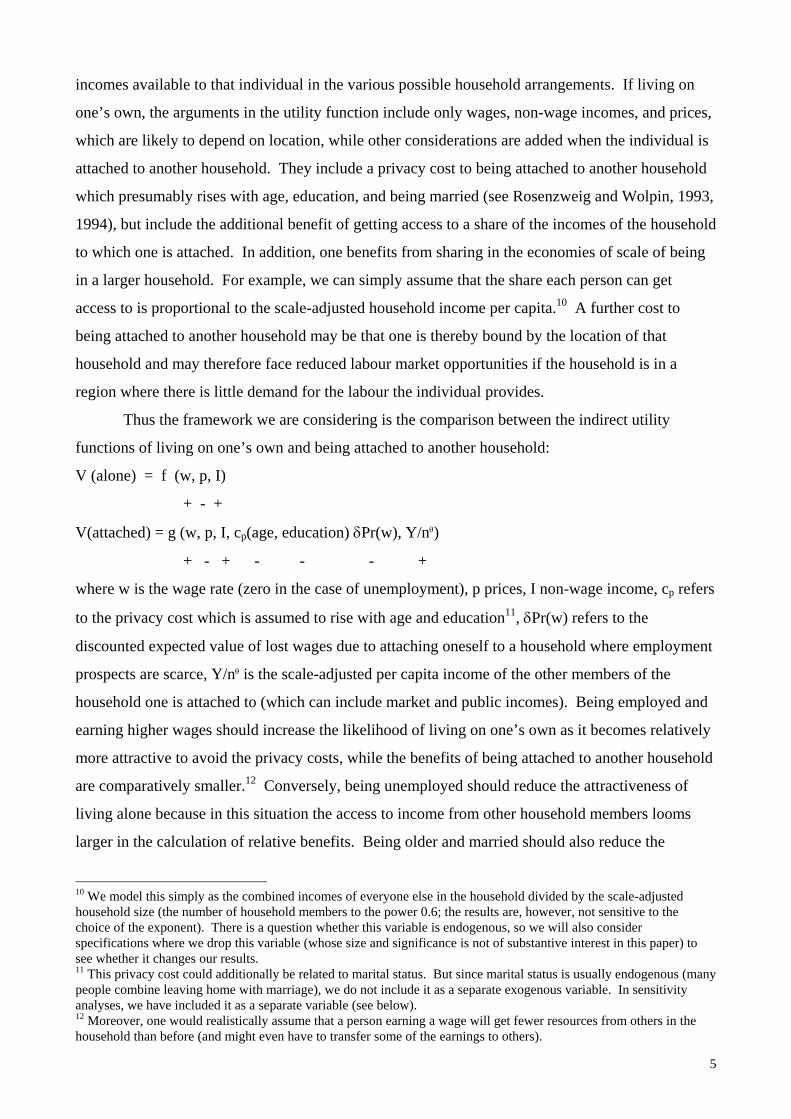
Thus the framework we are considering is the comparison between the indirect utility
functions of living on one’s own and being attached to another household:
V (alone) = f (w, p, I)
+ - +
V(attached) = g (w, p, I, cp(age, education) δPr(w), Y/nθ)
+ - + - - - +
where w is the wage rate (zero in the case of unemployment), p prices, I non-wage income, cp refers
to the privacy cost which is assumed to rise with age and education11, δPr(w) refers to the
discounted expected value of lost wages due to attaching oneself to a household where employment
prospects are scarce, Y/nθ is the scale-adjusted per capita income of the other members of the
household one is attached to (which can include market and public incomes). Being employed and
earning higher wages should increase the likelihood of living on one’s own as it becomes relatively
more attractive to avoid the privacy costs, while the benefits of being attached to another household
are comparatively smaller.12 Conversely, being unemployed should reduce the attractiveness of
living alone because in this situation the access to income from other household members looms
larger in the calculation of relative benefits. Being older and married should also reduce the
10 We model this simply as the combined incomes of everyone else in the household divided by the scale-adjusted household size (the number of household members to the power 0.6; the results are, however, not sensitive to the choice of the exponent). There is a question whether this variable is endogenous, so we will also consider specifications where we drop this variable (whose size and significance is not of substantive interest in this paper) to see whether it changes our results. 11 This privacy cost could additionally be related to marital status. But since marital status is usually endogenous (many people combine leaving home with marriage), we do not include it as a separate exogenous variable. In sensitivity analyses, we have included it as a separate variable (see below). 12 Moreover, one would realistically assume that a person earning a wage will get fewer resources from others in the household than before (and might even have to transfer some of the earnings to others).

6
likelihood of being attached, while higher (scale adjusted) per capita incomes of the receiving
household should increase the likelihood of being attached. Finally, the costs of being attached to a
household in a poor labour market should matter less for unemployed people who already face poor
labour market opportunities as their forgone earnings are comparatively smaller.
This very simple framework should allow us to study how the unemployed in South Africa
cope with their fate which is examined in more detail in the next three sections.
3. Background and Data
It may be useful to briefly summarise some key features of the South African economy and
labour market. South Africa is a middle income country whose economy depends to a considerable
extent on mining and mineral activities, a sizeable manufacturing sector serving the domestic and
regional markets (about 20% of total employment), a large service sector (including a large
governmental sector), a comparatively small, capital-intensive, commercialised agricultural sector
and a very low-productivity, small-scale subsistence agricultural sector in the former homelands
(with all of agriculture producing about 5% of GDP and absorbing some 10% of employment). The
apartheid system in place until the transition to black majority rule in the early 1990s had profound
effects on the economy and the labour market including:13
• discriminatory access to employment in the formal labour market with Whites being
favoured by better education systems, job reservation policies, and residential and
workplace restrictions (pass laws);
• an increasing capital-intensity of production in all sectors of the economy, promoted by an
increasing shortage of skilled labour, subsidies on capital, and attempts by the apartheid
state to lessen the dependence of the ‘White’ economy on unskilled African labour;
• restrictions on the movement of Africans (through pass laws and restrictions on housing and
urban amenities) forcing the majority of Africans into the homelands; this also contributed
to the splitting up of households where working-age members would be allowed to live and
work in the cities of white RSA and their dependants would be forced to reside in the
homelands and be dependent on remittances;
• several legislative measures to eliminate the previously widespread practise of share-
cropping, and ‘squatting’ of Africans on white-owned land14; and
• prohibitions and restrictions on formal and informal economic activities by Africans,
especially for those residing in non-homeland South Africa. 13 See Lundahl (1991), Fallon (1993), Fallon and Lucas (1997), Kingdon and Knight (2004), and ILO (1996) for details. 14 Squatting was an arrangement where Africans rented a portion of the land (or sometimes, the entire farm was rented
7
Partly as a result of the inefficiencies and distortions generated by some of the above
policies, per capita growth declined dramatically from 5% in the 1960s to 2% in the 1980s and less
than that in the 1990s. Employment growth fell to 0.7% in the 1980s and turned negative in the
1990s.15
With the labour force growing at about 2.5% per year, low employment growth ensured that
unemployment increased very rapidly in the 1980s and, by the 1990s reached the levels observed in
Table 1. Moreover, the apartheid legacy (especially with regards to education and the labour
market) is responsible for the fact that unemployment, employment, and earnings continue to differ
greatly by race which is a more important predictor of employment prospects and wages than any
other factor (including age, gender, education, experience, or location, see Klasen, 2002, and
Fallon and Lucas, 1997). 16 The decline in job creation in the 1980s and 1990s also contributed to
the steep age profile of unemployment (Klasen and Woolard, 1999, 2000; Kingdon and Knight,
2004). Lastly, apartheid policies are also largely responsible for the uneven population distribution
of Africans, many of whom (including most of the elderly) are still crowded in the predominantly
rural areas of the former homelands.
Despite the lack of a system of unemployment support or other safety nets targeted at the
unemployed, the one source of social security in South Africa comes in the form of fairly generous
non-contributory means-tested old-age pensions (Case and Deaton, 1998, Ardington and Lund,
1995). These pensions, originally intended for poor white elderly, were extended to all races at the
same level of benefits in the early 1990s and now are primarily a near-universal grant to elderly
Africans (the majority of whom qualify, while a significant share of the elderly of other race groups
are not eligible due to other incomes). The pensions have been maintained at these high levels
(about twice the level of median per capita income) in real terms ever since. Since many of the
elderly live in rural areas, particularly in the former homelands, these pensions support many
households in those areas, a subject examined in greater detail below.17
In our empirical analysis, we draw on cross-sectional household survey data from several
out in this way) and paid a fixed rent for doing so. For a discussion see Wilson (1971). 15 Some observers have also pointed to increasing capital intensity, rising union wage premia, and a number of external shocks (falling gold prices and financial sanctions) as further factors causing the slowdown in employment growth in the 1980s (e.g. Fallon and Lucas, 1997). 16 This predominance of race as a factor 10 years after the end of all statutory racial discrimination in the labour market (influx controls, job reservations, and colour bars were lifted in the 1980s), is mostly related to vastly different quality of education (Case and Deaton, 1999), the continued impact of past discrimination in the labour market which still has a powerful influence on the shape of the existing labour force, some persisting discrimination in the labour market (likely to have persisted until the early 1990s at least), and the absence of any significant job creation which could have hastened a change in the racial composition of the labour force. See also Klasen (2002). 17 More recently, a means-tested child support grant of smaller magnitude was introduced. For details, see Agüero et al. (2006).
8
years, always presenting the most up-to-date information available. Most of our descriptive data
come from the 2004 Labour Force Survey (LFS), while much of the econometric analysis is based
on the 1995 October Household Survey (OHS) linked to an Income and Expenditure Survey (IES)
or the 1993 South African Living Standards Survey (SALSS) as only these older surveys have all
the required information on household structure, location, employment, reservation wages, and
incomes that we need for the econometric assessment.18 While this mismatch in surveys is
regrettable, the great similarity in the basic patterns of the relationship between unemployment and
household structure between the surveys in the 1990s and today’s surveys suggest that the basic
behavioural patterns that have emerged to deal with high unemployment are essentially the same, so
that our findings from the older data appear to have great relevance for understanding South
Africa’s current unemployment problems.
In order to learn more about the dynamics of household formation and its interaction with
labour market trends, we also examine two waves from the KwaZulu-Natal Income Dynamics
Study which re-surveyed Africans and Indians from KwaZulu-Natal, South Africa’s most populous
province, that were included in the 1993 SALSS in 1993 and 2004.19
4. Descriptive Statistics
In motivating the econometric analysis, this section provides descriptive statistics on how
the unemployed are able to get access to resources despite the near absence of unemployment
insurance.20 This can be done using a person-level and household-level analysis. The former
investigates in what types of households unemployed individuals live; the latter asks what share of
households contain various combinations of employed and unemployed individuals.
Both analyses are shown in Table 2. The person-level analysis shows that in 2004 slightly
over 50% of the unemployed lived in households where someone is employed; another 11% of the
unemployed lived in households which received remittances from an absent household member.
This is largely related to the legacy of the migrant labour system created by apartheid era
restrictions on movements. Thus about 62% of the unemployed are able to depend on labour
income from a present (or absent) household member and about 38% of all unemployed live in
households with no connection to the labour market whatsoever. The disconnection from the
labour market for the unemployed has increased over time. In 1993 some 60% lived in a household
with a working member, 20% in households with remittances, and only 20% had no connection to
the labour market (see below and Klasen and Woolard, 2001).
18 The later surveys either lack income information, information on location, or information on household structure. 19 For details on this re-survey, refer to May et al. (2000). 20 See ILO (1996) and Fallon and Lucas (1997) for a similar, but somewhat more cursory analysis.
9
The bottom panel of Table 2 presents the household-level analysis, thus showing the
distribution of the employed and unemployed among households. The table shows that, despite
high unemployment, the majority of households (58%) contain not a single unemployed person.21
28% of households contains one unemployed person, and 13% 2-3 unemployed members,
suggesting that these households are severely burdened by the presence of unemployed members.
The table also shows that 24% of households receive neither labour income nor remittances and are
thus disconnected from the labour market. Particularly worrying is that about half of the households
with 2 or more unemployed members belong to that category of households disconnected from the
labour market. Trends over time show that the burden of unemployment has increased on many
households. As shown in Table 3, the share of households containing not a single unemployed
person has fallen from 70% in 1993 to 57% in 2004, and, correspondingly, the shares of households
with one, two, three, or more unemployed have all increased by 40-50% in that time period.
The two analyses suggest four findings. First, the unemployed are relatively widely
distributed across households, certainly much more widely than in rich countries (e.g. OECD,
1998). In the South African context, this is particularly surprising given that, due to racial
differences in unemployment, White households (and, to a lesser extent, Indian households) are
largely insulated from the burden of unemployment.22 This implies that among African households,
the burden of unemployment is particularly widely dispersed, with nearly 50% of households
housing at least one unemployed person, and quite a few more than one.
Second, the most important source of resources for the unemployed are labour incomes of
other household members, either directly from working household members or indirectly via
remittances from absent household members.23 Third, the burden of unemployment on the
unemployed and the households hosting them has increased over time. The share of unemployed
living in households with no connection to the labour market has markedly increased over time, as
has the share of households containing an unemployed person. Lastly, the burden is apportioned
unequally. A minority of households, many of which have little connection to the labour market
themselves, house a majority of unemployed and thus carry a disproportionate burden, while the
majority of households is not affected.
How do the unemployed survive in households without labour market connections? Table 2
shows that the majority of those households receive social grants, the vast majority of which are the
social pensions discussed above. Thus the public safety net complements the private safety net and 21 Given the racial differences in unemployment rates and the near absence of interracial households, most White and Indian, and a large share of Coloured households are among this group of households. 22 90% of White and 75% of Indian households did not contain an unemployed person in 2004. 23 As shown in Table 2, the role of remittances as a source of income has decreased over time which is related to the slow dismantling of the legacy of apartheid-era spatial policies that previously had restricted access of non-working
10
plays a surprisingly large role in the support of the unemployed, given that its beneficiaries are
largely elderly and, to a smaller extent, children.
But some 13% of the unemployed (and about 9% of households) have no access to labour
incomes or grants. How do these households survive? Data from the SALSS (1993) show that the
majority of these households eke out a very meagre existence based on small-scale agriculture
activities, minor self-employment or minor wage income (for less than 5 hours a week) or report no
incomes at all. These households earned on average some $115 per household per month, placing
them in the bottom decile of the income distribution.24
This section has shown that the private safety net of other household members, assisted by
the public safety to pensioners, ensures that the vast majority of the unemployed have indirect
access to labour or grant incomes. But this access is very unequal on the unemployed as well as the
households hosting them. Those unemployed not covered by these incomes sources have to
contend with abject poverty, and some households carry a much larger burden than others. The
process by which this private and public safety net ensures access to resources to the vast majority
of the unemployed deserves some further analysis which is taken up in the next section. 5. Unemployment and Household Formation: Evidence
In this section we investigate to what extent the dispersion of unemployment among
households is a result of explicit household formation strategies of the employed and the
unemployed.
In an exploratory analysis in Table 4, we have classified persons of working age according
to their position in the household which we measure via their relationship to the household head. If
we hypothesise that unemployed persons are likely to attach themselves to another household to
seek support we would not expect many unemployed to be household heads or spouses of the head
but instead to be living with their parents or other relatives (and thus their relation to the household
head would be child, sister, cousin, nephew, or niece of the household head). Conversely, we
would hypothesize that the employed are much more likely to found and head new households as
the have their own source of support and thus the privacy costs of remaining attached to another
household loom relatively large.25
Using the 1995 OHS and IES, we sort all possible relationships to the household head into
five groups: they are either the household head or his/her spouse (‘head/spouse’ in Table 4), they
are children younger than 25 years living with their parents (‘kid<25’), children age 25 or older
living with their parents (‘kid>25’), people living with siblings, living with other family (e.g. they family members to urban areas. 24 See Klasen and Woolard (2001) for more details.
11
are nephew, niece, cousin, parent, grandparents, uncle, aunt, or grandchildren of the household
head) or non-family.
Before proceeding to interpret the results, it is important to consider whether the definition
of a household head is an exogenous category within a given household or is itself dependent on
employment and income status of its members. While we cannot examine this using these cross-
sectional surveys, we can examine a two-wave panel from South Africa for 1993 and 1998, where
the African and Indian respondents in the 1993 SALSS survey from the province of KwaZulu-
Natal, were re-interviewed in 1998 to see whether the household head changed within a given
household configuration.26 If we restrict our analysis to households where the head in 1993 was
resident and was still alive in 1998, 96% of household heads or spouses in 1993 were still head or
spouse in 1998, and the very few who were ‘demoted’ from headship had an average age of 67.
Thus the definition of headship seems very stable and we can treat it as a category that is exogenous
to employment and earnings of individual members and thus can be seen to provide an accurate
reflection of household formation patterns.27
Table 4 shows that 75% of those employed are either household heads or their spouses,
suggesting that employment ensures that people can set up independent households. We compare
this to the strict and broad unemployed.28 In contrast to employed people, for the strictly (broadly)
unemployed, only 30 (32%) of them head households or are married to household heads, while a
surprising 26% (25%) of them are children aged 25 or over still living with their parents. Another
26% (25%) are children below 25 living with their parents, and 7% (7%) live with siblings, aunts,
or cousins, and another 10% (10%) live with other family.
Thus the unemployed appear to have a lower propensity to set up their own households;
instead they stay with their parents, or move in with close (or more distant) relatives. This is
similar to findings from the USA on the impact of welfare payments on location choices of single
mothers, and to findings from Southern Europe where particularly unemployed males stay often
until their 30’s with their parents.29
To investigate this issue further and place it in the context of the theoretical framework
discussed in section 2, we specify a multinomial logit model predicting the likelihood of each
relationship to the household head which, as discussed above, we believe gives an accurate
25 Also, they might then be forced to forgo some of their earnings to support other household members. 26 The third wave of the survey did not ask the household to specify the current head of the household – all relationship codes were specified relative to the 1993 head, regardless of his/her residency or vital status. 27 For a discussion of the concept of ‘household headship’ in South African surveys, see Budlender (1997). 28 To investigate the difference between those two types of unemployed, we treat the two categories throughout the subsequent analysis as exclusive categories, i.e. the broad unemployed only include those that are willing to work but have given up looking, and the strict only those that want to work and are actively searching. 29 See Ellwood and Bane (1985) and Rosenzweig and Wolpin (1993, 1994) for the US and Gallie and Paugham (2000) for Southern Europe.
12
reflection of household formation patterns. We distinguish between various destination states
including being household head or spouse of the household head (reference category), being a child
living with his/her parents, living with other family and living with non-family.30
We restrict the sample to people in the labour force, thus excluding the inactives and use a
dummy variable for the broadly unemployed to determine the effect of unemployment on household
formation.31 In line with the discussion in section 2, the regressions also control for age, education,
race, and the scale-adjusted per capita income of the household one is located in.32 The regressions
are estimated separately for males and females. Table 5 shows the descriptive statistics for the
variables used in the model. Using these regressions, we can then predict to what extent
employment status affects the relationship to the household head and thus household formation.
This type of analysis examines only the end results of the link between employment and the
relationship to household head and can say little about the process that created this outcome. It is
possible that employment enabled people to set up their own households, leaving the unemployed
to stay with parents or other relatives. In addition, the unemployed may have moved back to their
parents or relatives in response to unemployment. We will investigate this issue further by
examining information about migration in the various surveys, as well as consider qualitative
evidence from other disciplines.
Table 6 shows the results for the multinomial logit, separately for males and females. The
results confirm some of the findings of the theoretical discussion. Turning first to the regression for
males, age has the predicted effect of increasing the likelihood of heading one’s own household.
The influence of income is also as expected; the higher the household income, the more attractive it
is to be attached to such a household rather than setting up one’s own.33 Education has a varying
influence on household formation. While higher levels of education increase the chance of living
with one’s parents for both males and females, it has no impact on living with other relatives or
non-family, all compared to being household head or spouse.34 Ceteris paribus, race also has a
30 Most of the regressions do not violate the independence of irrelevant alternatives condition, as determined by a series of Hausman tests. See notes below the tables. 31 The relationship to the household head of the inactives is very much dependent on the reason for their inactivity (e.g. whether it is due to formal education, domestic responsibilities, disability, or retirement). 32 This is net of one’s own income to give a sense of how many additional resources one may be able to draw upon. Since this variable is partly endogenous to the household formation process (in a one-person household that variable is by definition zero; but one-person households are quite rare in South Africa), we also specify specifications without this variable to see if it affects the other coefficients (which it does not to any significant extent). 33 This finding should be treated with some caution as this variable, per capita income net of other household members, is partly endogenous to the household formation process (e.g. if one moves out and lives alone, a rare occurrence among Africans in South Africa, it will be zero). But inclusion of the income variable has no impact on the employment status variables, our main focus of interest. If we drop the income variable, unemployment has an even (slightly) stronger impact of remaining in the parental household or staying with relatives. These results are available upon request. 34 This may appear surprising as one would expect poorly educated people to be more likely to stay with the parents. But it appears that this effect is being counteracted by the fact that younger people are better educated (to the recent
13
sizable impact on household formation patterns. Compared to whites, all three other race groups
are much more likely to stay with their parents longer. Also, they are much more likely to live in
extended families, which can be seen in the table as the greater likelihood to live in a household
headed by a sibling, aunt, uncle, or grandfather. Only Africans and Coloureds are also significantly
more likely to live with non-family than whites. These racial differences probably point to cultural
differences in household formation patterns and the acceptability to shift household boundaries as a
way to share transfer resources (e.g. du Toit and Neves, 2006; Sagner and Mtati, 1999; Spiegel et
al. 1996).
For the purposes of this analysis, it is particularly important to see that being (broadly)
unemployed significantly reduces the chance of being household head or spouse.35 For males, the
impact of this variable is very large and very precisely determined leading and thus highly
significant, particularly with regard to remaining in the parental household or the household of
relatives. Thus the results from the cross-tabulations in Table 4 carry over to the multivariate
context. Unemployment either prevents the setting up of a household or leads the unemployed to
attach themselves to other households in search of support.
Interacting unemployment with race (not shown) shows a stronger effect of African
unemployed to live with parents and other family, but the reduced likelihood of unemployed people
setting up their own household is present, sizable, and significant for all races.36
In separate regressions (not shown) we additionally include marital status as an additional
regressor to see whether the impact of unemployment on household formation remains. As to be
expected, marital status has a very strong impact on household formation, with married males being
much less likely to live with their parents or other relatives. At the same time, the impact of
unemployment on household formation remains strong and highly significant with the coefficient
being only some 20% smaller than before. This suggests, on the one hand, that employment,
marriage, and the setting up of an independent household for males are often closely related. On
the other hand, the impact of employment on household formation remains strong even if we
control for marital status. Since we believe that employment affects the propensity for marriage
and associated household formation (by giving the employed the ability to finance a couple and
family) marriage is an endogenous variable. We thus prefer the specification in Table 6 as the one
that shows the total impact of employment on household formation, regardless of whether that
impact is mediated via marriage or not.
educational expansion) and more likely to be unemployed (compared to older cohorts) and thus forced to continue residing with their parents. 35 Considering only the narrowly unemployed, or both separately, leads to very similar results. See Klasen and Woolard (2001) for results. 36 The results are available on request.
14
For females the impact of unemployment on household formation is also strong and
significant but the coefficient is much smaller than for males, presumably due to the fact that it is
easier for an unemployed female to be spouse of a household head than for an unemployed male to
be household head. This is also confirmed by the regression where we include marital status as an
additional regressor. In contrast to males, for females the impact of unemployment on household
formation now increases, suggesting that, for females, unemployment and marriage is positively
correlated. But otherwise the same household formation effects are still present.
This importance of the link between unemployment and household formation is shown in
some simulations in Table 7. We compare the simulated effects of being employed, differentiating
between African and Whites, and being unemployed on household formation. Ceteris paribus, the
switch from being employed to being unemployed reduces the chance of being household head or
spouse by about 30 percentage points, which is considerably larger than all other effects in the
regression, including the large racial differences in household structure. Instead the unemployed
have a much higher propensity of living with their parents, although living with other family is also
considerably more likely for them. The simulated effects are, in line with findings from Table 6,
smaller for women but still present.
To what extent is this result driven by active migration in response to unemployment, or is it
the failure of young unemployed people to leave the home of parents or relatives that is driving the
results? The OHS contains information on recent migration (last 12 months) and birthplace
migration, but unfortunately does not state reasons for the migration. Both are not optimal
indicators of past household formation. Migration in the last 12 months covers too short a time
period and only affects 3% of the sample, while birthplace migration (i.e. migration away from
community where one was born in) also includes migration unrelated to household formation. 37
But they show quite similar pattern. In the top panel of Table 8, migration in the last twelve months
is related to employment and household formation. Those who are employed are more likely to
have moved (3.9% versus 1.2% for broad and 2.3% for narrow unemployed) and, if they moved, to
be head of the household now. That is, their migration was associated with setting up a new
household. The broad and narrow unemployed, on the other hand, are much less likely to have
moved and a significant share of those that moved did so to join the households of parents or other
relatives. They did presumably to draw on the support available. The birthplace migration
information yields exactly the same patterns, but with higher rates of migration. Among those who
are in employment, nearly half have moved from their place of birth and over 90% of them now are
37 Note also that if people stayed in the same town but changed household, this will not be captured. Nore also that if children moved with their parents, we assume that this is not of relevance for our analysis as the children did not change household and thus we treat them as if they had not moved.
15
household heads or spouse. Among the unemployed, the propensity to move is much smaller. Only
20-25% of each group has moved. The vast majority who have not moved remained in their
parental household or in a household of other relatives. Thirdly, of those few unemployed that have
moved, about a third moved in with parents and other family.38 Thus unemployment is a powerful
force for persistence in the family of parents or other relatives to draw on their support. This
persistence generates considerable regional immobility as the children remain tied to their parental
location which, in the South African context, often involves a location in rural areas and/or the
former homelands. Thus this migration information suggests that the predominant household
formation response to unemployment involves staying with parents or other relatives, while a
considerable minority react to unemployment by attaching themselves to the household of relatives
and non-family, and some return to their parents.39
In the appendix we expand the multinominal logit model for males to distinguish within
each category (head/spouse, kid, other family, non-family) between those who have moved from
the town of their birth and those who remained (see appendix Tables 1, 2).40 Those in employment
are much more likely to be head of the households and much more likely to have moved than to
have stayed. Employment thus is highly associated with headship and with moving. In contrast,
the predominant response to unemployment is staying with one’s parents or other relatives, while a
significant minority move to join family and non-family, and some return to their parents.
The panel data from the KIDS survey allows us to see whether a change in employment
status has had an impact on changes in household formation, thus enabling us to study the dynamics
of household formation behaviour.41 Table 3 in the appendix shows the results. Those who were
employed in both periods or became employed between 1993 and 1998 were much more likely to
remain head of household or set up their own household, while those who remained unemployed or
had become unemployed predominantly remained with their parents.42 A small share returned to
their parents in search of support and a much larger share of those that became unemployed
remained or became attached to households headed by other family. This also supports the finding
that the largest household formation response to unemployment is to remain in the parental house 38 The relative high incidence of headship among unemployed who moved is mostly due to females who have joined a husband’s family; among males, it is much rarer. 39 While this is the most likely interpretation of the table, it is also possible that some of the unemployed who live as children could have returned to the parental home (and not be regarded as having migrated since their current place of residence is their place of birth) and also some might have moved with other family or non-family. Given the close correlation with employment status, the interpretation advanced above seems much more plausible. 40 The results for migration in the last year are very similar, but somewhat less precisely determined due to the much lower propensity to have moved. They are available on request. 41 With the 1998 resurvey, we have another data point on employment status and household formation, but only limited information on developments in-between. 42 To be sure this finding does not contradict the finding that household headship is a largely exogenous category as we have shown earlier. The people who have become head between 1993 and 1998 have done so because the household
16
while a significant minority adapt by attaching themselves to households of other family.
Evidence from case studies, ethnographic and sociological literature largely confirms our
empirical results and fills in some of the dynamics that we are imperfectly able to capture. For
example, du Toit and Neves (2006) report on case studies of return migration to a household of
relatives to seek support in the case of unemployment, particularly for people too poor to sustain
even short periods of unemployment in an urban area; they also confirm the greater importance of
delayed household formation for many unemployed young people, particularly in the former
homelands.43 In addition, Sagner and Mtati (1999) investigate pension sharing in South Africa and
show that high unemployment leads to considerable moral pressure on pensioners to support them
through co-residence44
The delayed household formation of the unemployed can also partly explain the puzzle of
unusually high rural unemployment rates in South Africa. Two issues are of particular relevance
here. First, due to the legacy of apartheid residential policies, most Africans were forced to reside
in the former homelands, most of which consisted of densely populated rural areas. As the next
generation grew up in these households, those that have not been able to find employment have
continued to live there, thus boosting rural unemployment rates particularly in the former
homelands. Second, this spatial residential pattern of the unemployed has been supported by the
generous social pensions programme for the elderly. Under apartheid, most elderly Africans were
forced to live in the homelands, even if they had had prior employment in cities of rural areas of
formerly ‘white’ South Africa.45 The social pension programme has granted them a means of
support there, usually their most important means of support. But given that most elderly reside in
large households containing two or three generations that largely live off these pensions (e.g. Case
and Deaton, 1998, Sagner and Mtati, 1999), these programs have, as also demonstrated above, been
a critical source of support for the unemployed, thus providing further incentives for them to remain
in, or return to rural areas.
While this can explain why many young people without employment stay in rural areas, it
cannot fully explain why they remain unemployed there. In particular, the question arises why,
given their rural location, they would not simply help with agricultural activities of their families or
hire themselves out as agricultural labourers, common strategies in most other developing countries.
But here again, peculiarities of the apartheid legacy play a role. As discussed in more detail in
Klasen and Woolard (1998, 1999) and Ramphele and Wilson (1989), available land for agricultural head from 1993 is no longer there ((s)he has died or moved away) or they have founded a new household. 43 See also Baber (1998) for a case study from the Northern province, and Sagner (1997). 44 The authors suggest that most pensioners do not consider this sharing ‘fair’ or as an act of ‘reciprocity’ but feel, in line with an African cultural ethos of interdependence and priority of family welfare, under moral pressure to help out, even though they believe that they deserve resource transfers from the young rather than providing resources to them.
17
activities in the homelands was so small that not much more than gardening activities could be
sustained, thus obviating the need for more family labour. Similarly, due to the systematic removal
of African share-croppers and tenants from ‘white’ South Africa, as well as restrictions on the
movement and residence of farm labourers, there was hardly any casual labour market for
agricultural labour in formerly ‘white’ South Africa (except close to former homelands) thus
making it very difficult for unemployed in the homelands to work as casual labourers in
agriculture.46
We have shown that unemployment prevents the setting up of an independent household
which, due to peculiarities of the South African situation, ensures that many unemployed end up
staying and remaining unemployed in rural areas, far away from most employment opportunities
and may thus provide a disincentive to search and find employment. In those rural areas, access to
education, training, credit, employment services are similarly poor so that the unemployed that
reside there have very little chance to stay connected to the labour market and improve their human
capital. Whether this has a noticeable effect on their employment prospects is investigated in the
next section.
6. The Consequences of Household Formation Decisions of the Unemployed
The analysis so far has suggested that location decisions of the unemployed are heavily
influenced by the availability of economic support which might often lead them to stay in
households in rural areas, particularly the former homelands, far away from places with the best
employment opportunities. In this section we want to examine two consequences of this household
formation behaviour. The first is to investigate the impact of this behaviour on the welfare of the
unemployed and the welfare of households hosting them. As already mentioned in section 4, this
private safety net that operates via household formation does not work for everyone. While most
unemployed are able to get access to resources this way and this is a significant welfare
improvement to the unemployed and society at large as destitution is avoided for most of the
unemployed, the amount of resources they have access to varies greatly and some unemployed,
particularly those without access to labour and grant incomes, face destitution. Thus this private
safety net, while essential and beneficial for most of the unemployed, generates considerable risks
for those who might have to rely on it. Ethnographic evidence from Spiegel (1996) finds that often
the poorest and most vulnerable have greater difficulties accessing this private safety net, which
would be consistent with the very low incomes of those not able to draw on this safety net. 45 For a discussion, see Klasen and Woolard (1998) and Klasen (2002). 46 The absence of a reliable casual agricultural labour market further intensified mechanization of ‘white’ agriculture, which was already induced by subsidies, trade policies, and cheap credit. See Klasen and Woolard (1998) for a
18
In addition, those who are the providers of the safety net also have to shoulder a
considerable burden for their willingness to support the unemployed. As shown in Table 2, this
burden is distributed rather unevenly, with over 14% of households hosting two or more
unemployed. The impact his has on poverty is shown in Table 10 where we present a simple
regression of annual household income per adult equivalent among Africans, using the 1995
Income and Expenditure Survey. Adding an unemployed member to a household reduces adult
equivalent expenditures by over R1600 (over R500 reduction for adding one more person based on
the household size coefficient, and nearly R1100 reduction for that person being unemployed). If
the household hosting the unemployed is in rural areas and headed by someone with poor
education, having an average household size (5 people), two of whom are unemployed, this will, on
average, place that household far below the poverty line, which stood at about R3000 annual
income per person in 1995. As a result, there is a close correlation between hosting unemployed
people and poverty. In 1995 some 65% of the broad and 59% of the narrow unemployed found
themselves in households situated in the poorest two quintiles (defined by adult equivalent
expenditures). 51% of the people in the poorest quintile live in households where no one is
employed and only 17% of the working age population in the lowest quintile actually have a job.
As already shown in Table 3, the strain on this private safety net has increased over time as
more households have to host more unemployed members. The impact of this increasing strain is
also demonstrated in Woolard and Klasen (2005) who use the KIDS panel data and show that
hosting an unemployed member in 1993 or adding an unemployed member to a household between
1993 and 1998 are among the most important correlates of a decline into poverty between 1993 and
1998.47 Ethnographic and case study evidence also supports the strain being felt by the receiving
households who feel they are paying a heavy price for the moral obligation to help their kin.48
Another consequence of the location decision of the unemployed is the potential impact on
search behaviour. Since labour market decisions are often influenced by other household members,
we examine participation and search decisions as well as employment prospects at the household
level. In particular, we estimate a model predicting participation in the labour force, search
activities, and employment prospects based on income sources of the household and other labour
market characteristics. The first regression could indicate to what extent households rely on the
labour market for resources, the second gives an impression of the influences on search costs for the
unemployed, and the third should shed some light on the ability to get employment offers and on
discussion. 47 On the other hand, the new widespread availability of child grants for poor parents since 2000 is, alongside the continued access to generous old age pensions likely, however, to have helped to relieve this strain on households hosting unemployed members. 48 See, for example, Sagner and Mtati (1999) and du Toit and Neves (2006).
19
the willingness to accept such offers.
Since we specify the model at the household level, we try to predict the share of adults in a
household who report to be in the broad labour force (regression 1 in Table 10), the share of those
in the broad labour force who are also in the narrow labour force (employed or searching,
regression 2), and the share of those in the narrow labour force who are employed (regression 3),
respectively.49 Since the causality between remittance income and labour market behaviour may
run in both directions (i.e. household may receive remittance income because they have no one
employed), we have used the existence of an absent members of a household as an instrument for
remittance income and estimate the model using Two Stage Least Squares.50
The results in Table 10 show that age, education, gender, and location have the expected
signs and are all significant. Remittance income is negatively correlated with labour force
participation, search activities, and employment prospects. Similarly, pension and non-wage
private income in the household are also correlated with lower labour force participation, search
activities, and employment prospects of the adult household members. This effect is strongest in
the second regression suggesting that these income sources have the strongest impact on reducing
search activities. Since some 31% of all household containing unemployed people receive such
state support, this finding should be of some concern to policy-makers.51
These findings could either mean that remittance, pension and non-wage private income
provide a direct disincentive by raising the reservation wage. 52 Alternatively, they could mean that
unemployed people attach themselves to households with pension or remittance income, which
might reduce search activities and employment prospects if the household receiving pensions and
remittances is in rural areas.53 This could be due to high search costs there which reduce search
49 We also examined this using a person-level analysis trying to predict which broadly unemployed decide to search. The results suggest that poorly educated Africans in rural areas are least likely to search, confirming that being ‘stuck’ in rural areas significantly reduces employment prospects. The results are available on request. 50 As a benchmark, we ran Ordinary Least Squares regressions using the same variables (and without the instrument). The coefficients do not differ much from the OLS regressions. The instrument passes tests for relevance (it significantly influences the remittance variable proxied for) and exogeneity (in the sense that it does not influence the dependent variable, except through its influence on remittances). 51 Similarly, some 35% of the unemployed live in households which receive state support. 52 It should, however, be pointed out that pension income is likely to have fewer disincentive effects than other forms of support to the unemployed (such as direct unemployment benefits) as the pension income of an elderly member of the household will not be reduced when an adult member of the household finds employment. Bertrand et al. (2003) do, however, suggest that there might be small disincentive effects associated with pension receipt, although this finding is controversial (see Posel et al. 2004). 53 The negative coefficients on household incomes do not mean that these forms of income serve to increase unemployment. In fact, to the extent that pension, private, and remittance income reduces labour force participation, it contributes to lowering the unemployment rate as it reduces labour supply and relieves pressure on the labour market; the negative coefficient in regression 3 also says nothing about influence on the unemployment rate but only says something about who among the narrow labour force is likely to get employment. Only to the extent that other household income (such as pension income) reduces search activities and employment of adult members of households, may it contribute to increasing the unemployment rate by raising reservation wages and by increasing rigidities in the labour market. An alternative interpretation could be that those with other forms of income are searching less actively
20
activities or due to low employment prospects which would lower employment rates. Given the
discussion above on the endogeneity of household formation, this latter interpretation is more likely
and does indeed suggest a pattern of household formation that takes some unemployed people away
from job prospects and into households with pensions and remittances in rural areas which then
causes them do cease searching.
To further examine whether pension and private incomes constitute a direct disincentive to
search by raising the reservation wage, we also examine the determinants of reservation wages of
the unemployed. Table 11 shows the results of the regressions for monthly reservation wages,
based on the 1993 SALSS survey. We use the Heckman correction for this regression to address
the sample selection bias of the reservation wage equation. We use a worker-specific (by province,
age, gender, and education group of the worker) local unemployment rate and urban location as
identifying variables for the selection equation. Although the regression coefficients do not differ
greatly between the OLS and the Heckman regression, the Likelihood Ratio test indicates that
selectivity is indeed a problem so that it was right to address the potential selectivity issue.
While province, race, gender, age, and education have large and significant impact on the
reservation wages (as one would expect), pension and remittance incomes do not appear to raise
reservation wages. Only self-employment income and private income is associated with higher
reservation wages. Thus we find little evidence of a direct disincentive effect of pension and
remittance income on search activities and employment prospects through higher reservation
wages.54
This provides further confirmation that the linkages between pension and remittance income
and search and employment prospects operates via changes in household formation rather than
directly via an increase in the reservation wage. The unemployed get stuck in rural households in
order to get support from pensions and remittances and thereby reduce their search and employment
prospects. The direct impact of household income on search and employment prospects, operating
via an increase in the reservation wage, does not appear to be of significant magnitude (and may not
exist at all).
7. Conclusion
We started out by posing a question about the factors that can explain the persistence of high
unemployment in South Africa without significant unemployment insurance.
and thereby are less successful in securing employment. 54 We know of no other study that has examined the impact of pensions on reservation wages; given the importance of the issue, the policy debates on the effects of pensions may take note of this finding.
21
We were able to show that the unemployed are dispersed widely among South African
households ensuring that most of the unemployed have access to employment income or state
transfers received by other household members. While this insures some resource access, this
private safety net does not cover everyone. Moreover, it drags many of the households supporting
unemployed people into poverty and involuntarily increases household sizes, with negative
consequences for the welfare of receiving households.
The mechanism allowing for the wide dispersion of the unemployed is through adjustments
in the household boundaries. Employment ensures the ability to set up independent households,
leaving the unemployed to stay in (or return to) the households of parents or other relatives. Given
that many of these households are in rural areas, and are being sustained by social pensions and
remittances, unemployed persons will remain in (or move to) rural areas to draw on these resources
and thereby reduce their search activities and employment prospects. Further analysis of who
particularly stays with relatives in rural areas suggests that, not surprisingly, particularly those with
poorer labour market prospects to begin with, are particularly reliant on this safety net.55 This
prolongs their unemployment spells and leads to the sustenance of rural unemployment which is not
related to rural labour markets but simply to the location decisions of the unemployed. While social
pensions and other state support thus are able to support the unemployed (among other poor people,
see Deaton and Case, 1998), they appear to contribute to lower labour market mobility and may,
from that perspective, be inferior to direct support to the unemployed person, wherever they are.56
At the same time, we find no evidence of a direct disincentive effect of household income
on reservation wages which supports our contention that the reduced search activity of households
receiving pension and remittance income is a result of the location decision of the unemployed.
Several important policy conclusions emerge from these findings. Firstly, unemployment
can persist at very high levels even in the absence of unemployment support. Secondly, a private
safety net can, in theory, partly replace public support for the unemployed. In the absence of a
public safety net, such a private safety net is clearly welfare-enhancing by avoided destitution for
the majority of the unemployed. But this private safety net does not cover everyone and leaves
some unemployed and their dependants mired in deep poverty. Moreover, the burden of supporting
55 In earlier analyses where we distinguished between whether people live with parents, other family, or non-family in rural or urban areas, we found that more educated people were more likely to live with relatives and non-family in urban areas and actively search for employment, while less educated were more likely to stay with parents in rural areas and were not actively looking for employment. To the extent that these variables are correlated with indicators of motivation and employability, they support the claim that the less employable are more likely to rely on support of relatives in rural areas. The results from Table 10 are also consistent with this claim as they show that education and urban location is associated with higher labour force participation, search intensity, and employment prospects. See also Klasen and Woolard (2001) and Sagner and Mtati (1999) for further support. 56 At the same time, there are other advantages to the social pensions as support for the unemployed, compared to unemployment insurance. In particular, they provide no direct disincentive effect. See also Case and Deaton (1998).
22
the unemployed is unequally distributed, pushing many households supporting the unemployed into
poverty. Finally, in the South African case, this private safety net heavily depends on the existence
of state transfers to pensioners which indirectly supports the unemployed.
Thirdly, reliance on a private safety net can generate disincentive effects that can prolong
unemployment. In particular, it forces the unemployed to base their location decisions on the
availability of economic support rather than on the best location for employment search. In the
South African case, where a lot of family support (partly sustained by the social pensions) is based
in rural areas, this leads to low labour market mobility, reduces search activities (since there are few
prospects of employment) and thus prolongs unemployment.
Developing policy options that remedy the deficiencies and incentive effects of this private
safety net are not easy to come by. To the extent it is the case that those with the worst labour
market prospects are predominantly covered by this private safety net in rural areas, one may even
argue that the current situation is the best one can hope for in a situation of high unemployment and
an imperfect public safety net. Then the main policy issue would be to ensure that the state
complements this private safety net by assisting those unemployed that have no means of private
support and by helping households manage the strain of supporting the unemployed. While an
extension of unemployment insurance could address these issues, it would come at a considerable
cost and might generate other disincentive effects.57 Simultaneously, efforts should be directed to
improve the job prospects of the unemployed, either through enhancing their education, skills, or
access to self-employment options.
At the same time, one should also consider policies to reduce the regional immobility and
increase search activities of the unemployed. While also here, policy solutions are not obvious,
some issues deserve a closer look. First, (financial and other) assistance for search and relocation
of the unemployed youth might be one way to overcome the barriers to search affecting many in
rural areas.58 Second, one could target training and public works programmes particularly to rural
unemployed youths to enable their transition into urban labour markets. Third, given the presence
of involuntary rural unemployment, efforts to revive small-scale agriculture and help re-create
casual labour markets in rural areas might be ways. The land reform programme is helpful here as
it intensifies agricultural production on smaller holdings and also recreates different size classes of
land-holdings which can create the preconditions for labour demand from larger farms and labour
supply from smaller ones. But implementation is slow, and it is, in any case, just a first step which
will need to be complemented by other policies (e.g. infrastructure and household policies) to re-
57 To mitigate some of these, one might consider payments or in-kind support to households housing unemployed members (similar to a child grant). 58 Also here, unemployment insurance would help but the same cautionary remarks apply.
23
create a casual labour market in rural areas (see Klasen and Woolard, 1998).
While many of these issues and problems are quite unique to the South African situation, the
general message of the workings and incentive effects of private safety nets for the unemployed
also are of relevance for other countries. For example, many of the processes observed of delayed
household formation of unemployed young people in South Africa have also been mentioned in an
explanation of a Southern European pattern of delayed household formation, particularly of young
males (e.g. Gallie and Paugham, 2000; Bentolila and Ichino, 2000).59 Also here, unemployment,
high housing costs, and no direct access to state support for unemployed young people leads to long
delays in household formation and resulting regional immobility and disincentive effects. It would
be fruitful if future research and policy analysis would try to explicitly consider the messages
emerging from the similar experience of unemployment and household formation in these two very
different settings.
Bibliography Agüero, Jorge, Carter, Michael and Ingrid Woolard. 2006. The Impact of Unconditional Cash Transfers on Nutrition: the case of the South African Child Support Grant. SALDRU Working Paper, University of Cape Town. Ardington, Elizabeth and Frances Lund. 1995. Pensions and Development: Social Security as Complementary to Programmes of Reconstruction and Development. Development Southern Africa, 12, no. 4. Arulampalam, Wiji, and Mark Stewart. 1995. ”The Determinants of Individual Unemployment Durations in an Era of High Unemployment.” Economic Journal 105: 321-332. Atkinson, Anthony B. and John Micklewright. 1991. Unemployment Compensation and Labor Market Transitions: A Critical Review. Journal of Economic Literature 29: 1679-1727. Bardhan, Pranab. 1978. ‘On Measuring Rural Unemployment’. Journal of Development Studies 342-352. Bentolila, Samuel and Andrea Ichino. 2000. ”Unemployment and Consumption: Are job losses less Painful near the Mediterrranean?” Florence: EUI, mimeographed. Bertrand, M., Mullainathan, S. and Miller, D. (2003) “Public Policy and Extended Families: Evidence from Pensions in South Africa”. The World Bank Economic Review 17 (1): 27 – 50. Blanchard, Olivier and James Wolfers. 2000. ”The Role of Shocks and Institutions in the Rise of European Unemployment: The Aggregate Evidence.” Economic Journal 110: C1-33. Börsch-Supan, Axel. 1986. ”Household Formation, Housing Prices, and Public Policy Impacts.”
59 See also Card and Lemieux (2000) for evidence for the USA.
24
Journal of Public Economics 30: 145-164. Card, David and Thomas Lemieux. 2000. Adapting to Circumstances: The Evolution of Work, School, and Living Arrangements among North American Youth. In Blanchflower, D. amd R. Freeman (eds.) Youth Employment and Joblessness in Advanced Countries. Chicago: University of Chicago Press. Case, Anne and Angus Deaton. 1998. ”Large Cash Transfers to the Elderly in South Africa.” Economic Journal 108: 1330-1363. ------. 1999. School Inputs and Educational Outcome in South Africa. Quarterly Journal of Economics 114:1047-1084. Du Toit, Andries and D. Neves. Vulnerability and Social Protection at the Margins of the Formal Economy. Pretoria: USAID. Edmonds, Eric V., Kristin Mammen, Douglas L. Miller. 2005. “Rearranging the Family? Income Support and Elderly Living Arrangements in a Low-Income Country.” Journal of Human Resources 40(1): 186-207. Ellwood, David and Lawrence Summers. 1986. ”Poverty in America: Is Welfare the Answer or the Problem?” in Danziger, Sheldon and Daniel Weinberg (eds.) Poverty, What Works and What Doesn’t. Cambridge: Harvard University Press. ------. and Mary Jo Bane. 1985. ”The Impact of AFDC on Family Structure and Living Arrangements,” in Ron Ehrenberg (ed.) Research in Labour Economics, Vol. 7. Greenwhich: JAI Press. Ermisch, John and Pamela di Salvo. 1997. ”The Economic Determinants of Young People’s Household Formation. Economica 64:627-644. Fallon, Peter. 1992. An Analysis of Employment and Wage Behavior in South Africa. Washington DC: The World Bank. -----, and Bob Lucas. 1997. South African Labour Markets: Adjustment and Inequality. Washington, DC: The World Bank. Gallie, Duncan and Serge Paugham. 2000. The Social Regulation of Unemployment. Oxford: Oxford University Press (forthcoming). Gregg, Paul and Jonatahn Wadsworth. 1996. ”It takes two: Employment Polarization in the OECD.” Centre for Economic Performance Discussion Paper No. 304. International Labour Organization. 1996. Restructuring the Labour Market: The South African Challenge. Geneva: ILO. International Labour Organization. 2005. Laboursta Database. Geneva: ILO. Kingdon, Geeta and John Knight. “The measurement of unemployment when unemployment is high”, Labour Economics , forthcoming 2006 -----. 2004. Unemployment in South Africa: Causes, Problems, and Policies. Mimeographed,
25
Oxford: Centre for the Study of African Economies. Klasen, Stephan. 2002. Social, economic, and environmental limits to the newly enfranchised in South Africa? Economic Development and Cultural Change 50:607-642. -----. 2000. Measuring Poverty and Deprivation in South Africa. Review of Income and Wealth. 46:33-58. -----, and Ingrid Woolard. 1998. Unemployment, household formation, poverty and nutrition in South Africa. Munich: University of Munich. Mimeographed. -----, and Ingrid Woolard. 1999. ‘Levels, Trends and Consistency of Measured Employment and Unemployment in South Africa.’ Development Southern Africa 16: 3-35. -----. 2000. Unemployment and Employment in South Africa, 1995-1997. Pretoria: Department of Finance. Mimeographed. -----. 2001. Surviving Unemployment without State Support: Unemployment and Household Formation in South Africa. CESifo Working Paper No. 533. Labour Market Commission. 1996. Report of the Labour Market Commission. Pretoria: Department of Labour. Lundahl, Mats. 1991. Apartheid in Theory and Practise. Boulder: Westview Press. May, Julian. 1996. Experiences and Perception of Poverty in South Africa. Durban: DRA. ----, et al. 1997. The South Africa Poverty and Inequality Report. Durban: DRA. May, J., Carter, M., Haddad, L. and J. Malluccio 2000, ‘Kwa-Zulu Natal Income Dynamics Study (KIDS) 1993-1998: A longitudinal household data set for Southern African policy analysis’, Development Southern Africa 17(4), 567-581. McElroy, Marjorie. 1985. ”The Joint Determinantion of Household Membership and Market Work: The case of Young Men.” Journal of Labor Economics 3: 293-316. Mortenson, Dale. 1977. ”Unemployment and Job Search Decisions.” Industrial and Labour Relations Review 30: 505-517. Murray, Charles P. 1984. Losing Ground. New York: Basic Books. Nickell, Stephen. 1997. ”Unemployment and Labor Market Rigidities: Europe versus North America”. Journal of Economic Perspectives 11: 55-74. OECD. 1998. Employment Outlook June 1998. Paris: OECD. Posel, D., J. A. Fairburn, and F. Lund. 2004 Labour Migration and Households: A Reconsideration of the Effects of the Social Pension on Labour Supply in South Africa. Mimeographed, University of Natal. Ramphele, Mamphele, and Francis Wilson. 1989. Uprooting Poverty: The South African Challenge.
26
New York: Norton. Rosenzweig, Mark and Kenneth Wolpin. 1993. ”Intergenerational Support and the Life-Cycle Incomes of Young Menand their Parents.” Journal of Labor Economics 11: 84-112. -----. 1994. ”Parental and Public Transfers to Young Women and their Children.” American Economic Review 84: 1195-1212. Sagner, A. 1997. Urbanization, ageing and migration. Southern African Journal of Gerontology 6: 13-19. Sagner, A. and R. Mtati. 1999. Politics of pension sharing in urban South Africa. Ageing and Society 19: 393-416. Saldru. 1993. The South African Living Standards and Development Survey. Cape Town: Saldru. Spiegel, A. V. Watson, and P Wilkinson. 1996. Domestic diversity and fluidity in some African households in Greater Cape Town. Social Dynamics 22: 7-30. Statistics South Africa (Stats SA). 1994, 1995, 1997, 1999. October Household Survey. Pretoria: Stats SA. Statistics South Africa (Stats SA). 2000, 2001, 2002, 2003, 2004. Labour Force Survey. Pretoria: Stats SA. Todaro, Michael and Stephen Smith. 2003. Economic Development. Edinburgh: Pearson Education Limited. Wilson, Francis. 1971. Farming, 1866-1966. in Wilson, M. and L. Thompson (eds) The Oxford History of South Africa. Oxford: Oxford University Press. Woolard, I. and S. Klasen. 2005. Determinants of Income Mobility and Household Poverty Dynamics in South Africa. Journal of Development Studies (forthcoming). World Bank. 1995. World Development Report. New York: Oxford University Press.
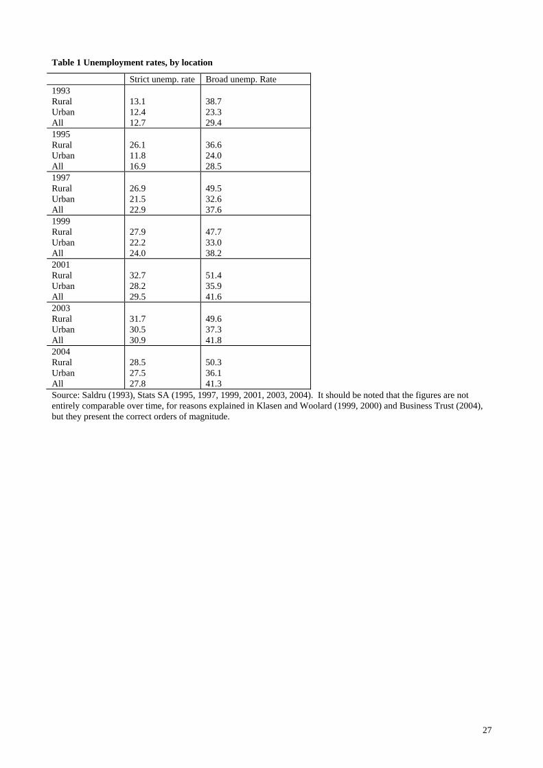
27
Table 1 Unemployment rates, by location Strict unemp. rate Broad unemp. Rate 1993 Rural Urban All
13.1 12.4 12.7
38.7 23.3 29.4
1995 Rural Urban All
26.1 11.8 16.9
36.6 24.0 28.5
1997 Rural Urban All
26.9 21.5 22.9
49.5 32.6 37.6
1999 Rural Urban All
27.9 22.2 24.0
47.7 33.0 38.2
2001 Rural Urban All
32.7 28.2 29.5
51.4 35.9 41.6
2003 Rural Urban All
31.7 30.5 30.9
49.6 37.3 41.8
2004 Rural Urban All
28.5 27.5 27.8
50.3 36.1 41.3
Source: Saldru (1993), Stats SA (1995, 1997, 1999, 2001, 2003, 2004). It should be noted that the figures are not entirely comparable over time, for reasons explained in Klasen and Woolard (1999, 2000) and Business Trust (2004), but they present the correct orders of magnitude.
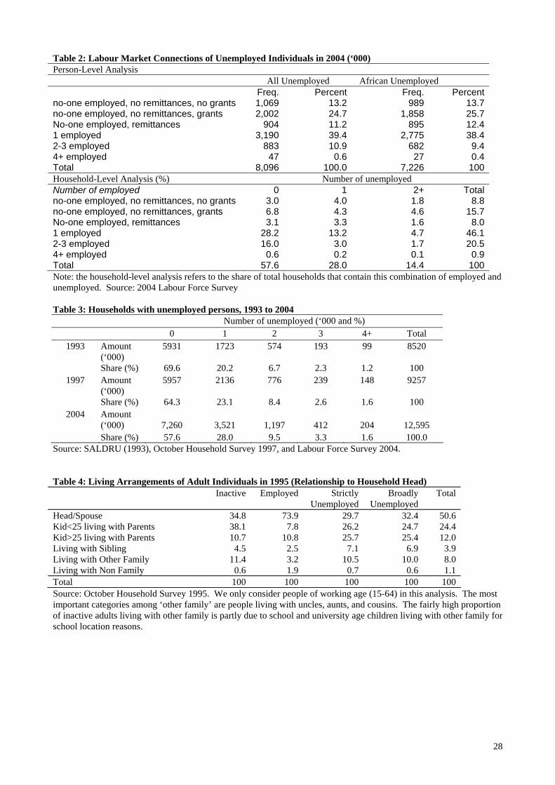
28
Table 2: Labour Market Connections of Unemployed Individuals in 2004 (‘000) Person-Level Analysis All Unemployed African Unemployed Freq. Percent Freq. Percent no-one employed, no remittances, no grants 1,069 13.2 989 13.7 no-one employed, no remittances, grants 2,002 24.7 1,858 25.7 No-one employed, remittances 904 11.2 895 12.4 1 employed 3,190 39.4 2,775 38.4 2-3 employed 883 10.9 682 9.4 4+ employed 47 0.6 27 0.4 Total 8,096 100.0 7,226 100 Household-Level Analysis (%) Number of unemployed Number of employed 0 1 2+ Total no-one employed, no remittances, no grants 3.0 4.0 1.8 8.8 no-one employed, no remittances, grants 6.8 4.3 4.6 15.7 No-one employed, remittances 3.1 3.3 1.6 8.0 1 employed 28.2 13.2 4.7 46.1 2-3 employed 16.0 3.0 1.7 20.5 4+ employed 0.6 0.2 0.1 0.9 Total 57.6 28.0 14.4 100Note: the household-level analysis refers to the share of total households that contain this combination of employed and unemployed. Source: 2004 Labour Force Survey Table 3: Households with unemployed persons, 1993 to 2004
Number of unemployed (‘000 and %) 0 1 2 3 4+ Total
1993 Amount (‘000)
5931 1723 574 193 99 8520
Share (%) 69.6 20.2 6.7 2.3 1.2 100 1997 Amount
(‘000) 5957 2136 776 239 148 9257
Share (%) 64.3 23.1 8.4 2.6 1.6 100 2004 Amount
(‘000) 7,260 3,521 1,197 412 204 12,595 Share (%) 57.6 28.0 9.5 3.3 1.6 100.0 Source: SALDRU (1993), October Household Survey 1997, and Labour Force Survey 2004. Table 4: Living Arrangements of Adult Individuals in 1995 (Relationship to Household Head) Inactive Employed Strictly
Unemployed Broadly
Unemployed Total
Head/Spouse 34.8 73.9 29.7 32.4 50.6 Kid<25 living with Parents 38.1 7.8 26.2 24.7 24.4 Kid>25 living with Parents 10.7 10.8 25.7 25.4 12.0 Living with Sibling 4.5 2.5 7.1 6.9 3.9 Living with Other Family 11.4 3.2 10.5 10.0 8.0 Living with Non Family 0.6 1.9 0.7 0.6 1.1 Total 100 100 100 100 100 Source: October Household Survey 1995. We only consider people of working age (15-64) in this analysis. The most important categories among ‘other family’ are people living with uncles, aunts, and cousins. The fairly high proportion of inactive adults living with other family is partly due to school and university age children living with other family for school location reasons.
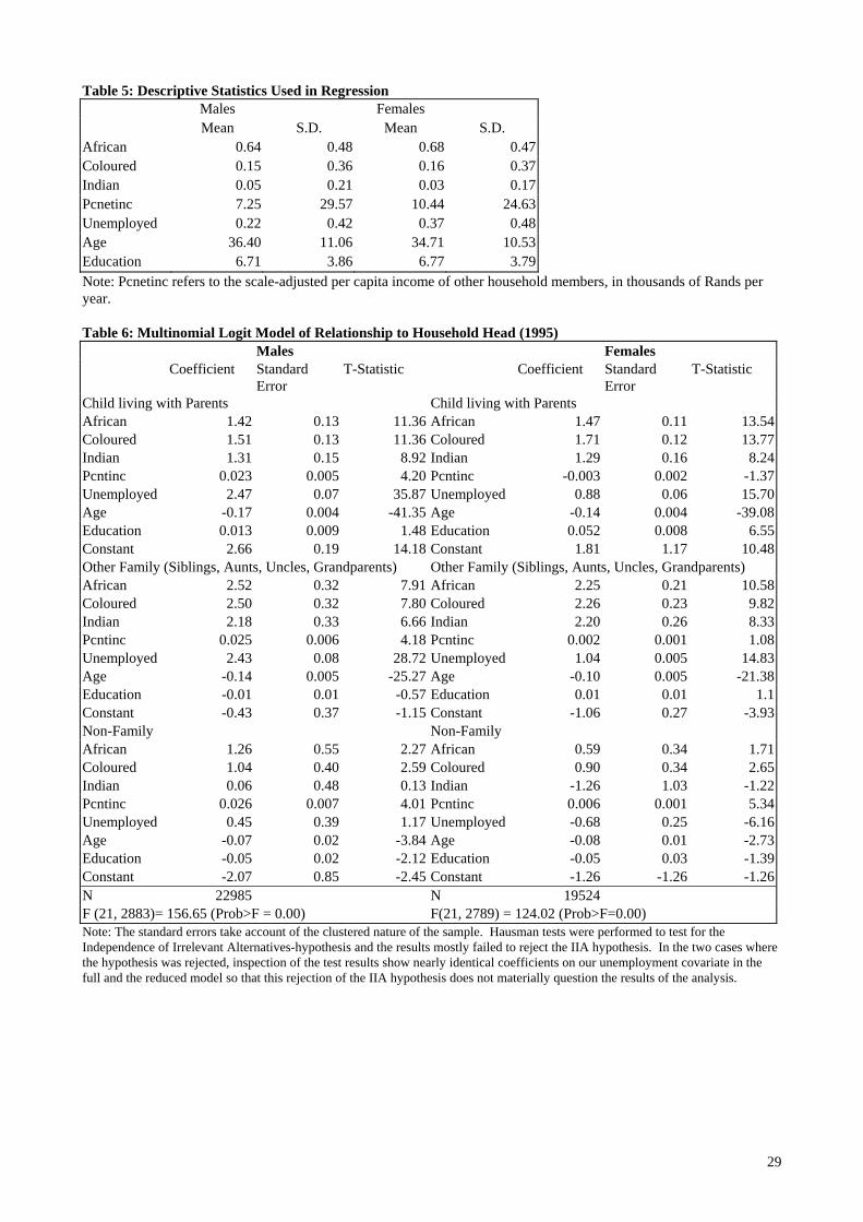
29
Table 5: Descriptive Statistics Used in Regression Males Females Mean S.D. Mean S.D.
African 0.64 0.48 0.68 0.47Coloured 0.15 0.36 0.16 0.37Indian 0.05 0.21 0.03 0.17Pcnetinc 7.25 29.57 10.44 24.63Unemployed 0.22 0.42 0.37 0.48Age 36.40 11.06 34.71 10.53Education 6.71 3.86 6.77 3.79Note: Pcnetinc refers to the scale-adjusted per capita income of other household members, in thousands of Rands per year. Table 6: Multinomial Logit Model of Relationship to Household Head (1995)
Males Females Coefficient Standard
Error T-Statistic Coefficient Standard
Error T-Statistic
Child living with Parents Child living with Parents African 1.42 0.13 11.36 African 1.47 0.11 13.54Coloured 1.51 0.13 11.36 Coloured 1.71 0.12 13.77Indian 1.31 0.15 8.92 Indian 1.29 0.16 8.24Pcntinc 0.023 0.005 4.20 Pcntinc -0.003 0.002 -1.37Unemployed 2.47 0.07 35.87 Unemployed 0.88 0.06 15.70Age -0.17 0.004 -41.35 Age -0.14 0.004 -39.08Education 0.013 0.009 1.48 Education 0.052 0.008 6.55Constant 2.66 0.19 14.18 Constant 1.81 1.17 10.48Other Family (Siblings, Aunts, Uncles, Grandparents) Other Family (Siblings, Aunts, Uncles, Grandparents) African 2.52 0.32 7.91 African 2.25 0.21 10.58Coloured 2.50 0.32 7.80 Coloured 2.26 0.23 9.82Indian 2.18 0.33 6.66 Indian 2.20 0.26 8.33Pcntinc 0.025 0.006 4.18 Pcntinc 0.002 0.001 1.08Unemployed 2.43 0.08 28.72 Unemployed 1.04 0.005 14.83Age -0.14 0.005 -25.27 Age -0.10 0.005 -21.38Education -0.01 0.01 -0.57 Education 0.01 0.01 1.1Constant -0.43 0.37 -1.15 Constant -1.06 0.27 -3.93Non-Family Non-Family African 1.26 0.55 2.27 African 0.59 0.34 1.71Coloured 1.04 0.40 2.59 Coloured 0.90 0.34 2.65Indian 0.06 0.48 0.13 Indian -1.26 1.03 -1.22Pcntinc 0.026 0.007 4.01 Pcntinc 0.006 0.001 5.34Unemployed 0.45 0.39 1.17 Unemployed -0.68 0.25 -6.16Age -0.07 0.02 -3.84 Age -0.08 0.01 -2.73Education -0.05 0.02 -2.12 Education -0.05 0.03 -1.39Constant -2.07 0.85 -2.45 Constant -1.26 -1.26 -1.26N 22985 N 19524 F (21, 2883)= 156.65 (Prob>F = 0.00) F(21, 2789) = 124.02 (Prob>F=0.00) Note: The standard errors take account of the clustered nature of the sample. Hausman tests were performed to test for the Independence of Irrelevant Alternatives-hypothesis and the results mostly failed to reject the IIA hypothesis. In the two cases where the hypothesis was rejected, inspection of the test results show nearly identical coefficients on our unemployment covariate in the full and the reduced model so that this rejection of the IIA hypothesis does not materially question the results of the analysis.
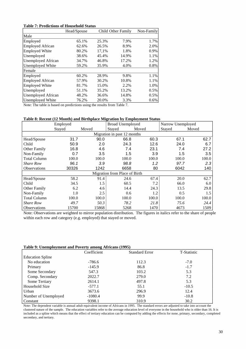
30
Table 7: Predictions of Household Status Head/Spouse Child Other Family Non-FamilyMale Employed 65.1% 25.3% 7.9% 1.7%Employed African 62.6% 26.5% 8.9% 2.0%Employed White 80.2% 17,1% 1.8% 0.9%Unemployed 38.6% 45.4% 14.9% 1.1%Unemployed African 34.7% 46.8% 17.2% 1.2%Unemployed White 59.2% 35.9% 4.0% 0.8%Female Employed 60.2% 28.9% 9.8% 1.1%Employed African 57.9% 30.2% 10.8% 1.1%Employed White 81.7% 15.0% 2.2% 1.0%Unemployed 51.1% 35.2% 13.2% 0.5%Unemployed African 48.2% 36.6% 14.8% 0.5%Unemployed White 76.2% 20.0% 3.3% 0.6%Note: The table is based on predictions using the results from Table 7. Table 8: Recent (12 Month) and Birthplace Migration by Employment Status Employed Broad Unemployed Narrow Unemployed Stayed Moved Stayed Moved Stayed Moved
Migration in past 12 months Head/Spouse 31.7 90.0 66.8 60.3 67.1 62.7Child 50.9 2.0 24.3 12.6 24.0 6.7Other Family 16.8 4.6 7.4 23.1 7.4 27.2Non-Family 0.7 3.5 1.5 3.9 1.5 3.5Total Column 100.0 100.0 100.0 100.0 100.0 100.0Share Row 96.1 3.9 98.8 1.2 97.7 2.3Observations 30326 1242 6658 80 6042 140
Migration from Place of Birth Head/Spouse 58.2 91.4 24.6 67.4 20.0 62.7Child 34.5 1.5 60.5 7.2 66.0 6.0Other Family 6.2 4.6 14.4 24.3 13.5 29.8Non-Family 1.0 2.5 0.6 1.2 0.5 1.5Total Column 100.0 100.0 100.0 100.0 100.0 100.0Share Row 49.7 50.3 78.2 21.8 75.6 24.4Observations 15700 15868 5268 1470 4673 1509Note: Observations are weighted to mirror population distribution. The figures in italics refer to the share of people within each row and category (e.g. employed) that stayed or moved. Table 9: Unemployment and Poverty among Africans (1995) Coefficient Standard Error T-Statistic Education Spline No education -786.6 112.3 -7.0 Primary -145.9 86.8 -1.7 Some Secondary 547.3 103.2 5.3 Comp. Secondary 2022.7 279.0 7.2 Some Tertiary 2614.1 497.8 5.3 Household Size -577.1 55.1 -10.5 Urban 3673.6 296.9 12.4 Number of Unemployed -1080.4 99.9 -10.8 Constant 9398.1 310.9 30.2 Note: The dependent variable is annual adult equivalent income of Africans in 1995. The standard errors are adjusted to take into account the clustered nature of the sample. The education variables refer to the average education level of everyone in the household who is older than 16. It is included as a spline which means that the effect of tertiary education can be computed by adding the effects for none, primary, secondary, completed secondary, and tertiary.
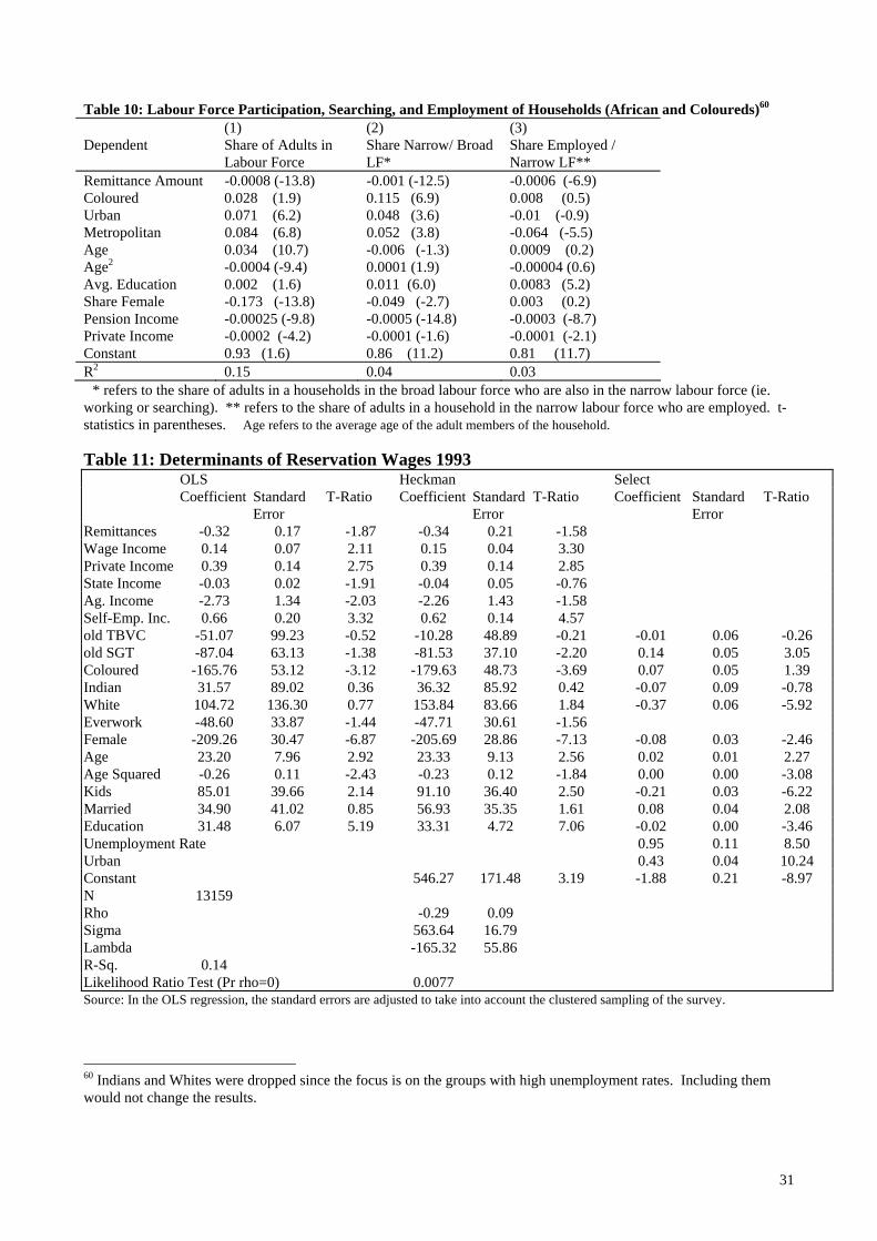
31
Table 10: Labour Force Participation, Searching, and Employment of Households (African and Coloureds)60 (1) (2) (3) Dependent Share of Adults in
Labour Force Share Narrow/ Broad LF*
Share Employed / Narrow LF**
Remittance Amount -0.0008 (-13.8) -0.001 (-12.5) -0.0006 (-6.9) Coloured 0.028 (1.9) 0.115 (6.9) 0.008 (0.5) Urban 0.071 (6.2) 0.048 (3.6) -0.01 (-0.9) Metropolitan 0.084 (6.8) 0.052 (3.8) -0.064 (-5.5) Age 0.034 (10.7) -0.006 (-1.3) 0.0009 (0.2) Age2 -0.0004 (-9.4) 0.0001 (1.9) -0.00004 (0.6) Avg. Education 0.002 (1.6) 0.011 (6.0) 0.0083 (5.2) Share Female -0.173 (-13.8) -0.049 (-2.7) 0.003 (0.2) Pension Income -0.00025 (-9.8) -0.0005 (-14.8) -0.0003 (-8.7) Private Income -0.0002 (-4.2) -0.0001 (-1.6) -0.0001 (-2.1) Constant 0.93 (1.6) 0.86 (11.2) 0.81 (11.7) R2 0.15 0.04 0.03 * refers to the share of adults in a households in the broad labour force who are also in the narrow labour force (ie. working or searching). ** refers to the share of adults in a household in the narrow labour force who are employed. t-statistics in parentheses. Age refers to the average age of the adult members of the household. Table 11: Determinants of Reservation Wages 1993
OLS Heckman Select Coefficient Standard
Error T-Ratio Coefficient Standard
Error T-Ratio Coefficient Standard
Error T-Ratio
Remittances -0.32 0.17 -1.87 -0.34 0.21 -1.58 Wage Income 0.14 0.07 2.11 0.15 0.04 3.30 Private Income 0.39 0.14 2.75 0.39 0.14 2.85 State Income -0.03 0.02 -1.91 -0.04 0.05 -0.76 Ag. Income -2.73 1.34 -2.03 -2.26 1.43 -1.58 Self-Emp. Inc. 0.66 0.20 3.32 0.62 0.14 4.57 old TBVC -51.07 99.23 -0.52 -10.28 48.89 -0.21 -0.01 0.06 -0.26 old SGT -87.04 63.13 -1.38 -81.53 37.10 -2.20 0.14 0.05 3.05 Coloured -165.76 53.12 -3.12 -179.63 48.73 -3.69 0.07 0.05 1.39 Indian 31.57 89.02 0.36 36.32 85.92 0.42 -0.07 0.09 -0.78 White 104.72 136.30 0.77 153.84 83.66 1.84 -0.37 0.06 -5.92 Everwork -48.60 33.87 -1.44 -47.71 30.61 -1.56 Female -209.26 30.47 -6.87 -205.69 28.86 -7.13 -0.08 0.03 -2.46 Age 23.20 7.96 2.92 23.33 9.13 2.56 0.02 0.01 2.27 Age Squared -0.26 0.11 -2.43 -0.23 0.12 -1.84 0.00 0.00 -3.08 Kids 85.01 39.66 2.14 91.10 36.40 2.50 -0.21 0.03 -6.22 Married 34.90 41.02 0.85 56.93 35.35 1.61 0.08 0.04 2.08 Education 31.48 6.07 5.19 33.31 4.72 7.06 -0.02 0.00 -3.46 Unemployment Rate 0.95 0.11 8.50 Urban 0.43 0.04 10.24 Constant 546.27 171.48 3.19 -1.88 0.21 -8.97 N 13159 Rho -0.29 0.09 Sigma 563.64 16.79 Lambda -165.32 55.86 R-Sq. 0.14 Likelihood Ratio Test (Pr rho=0) 0.0077 Source: In the OLS regression, the standard errors are adjusted to take into account the clustered sampling of the survey.
60 Indians and Whites were dropped since the focus is on the groups with high unemployment rates. Including them would not change the results.
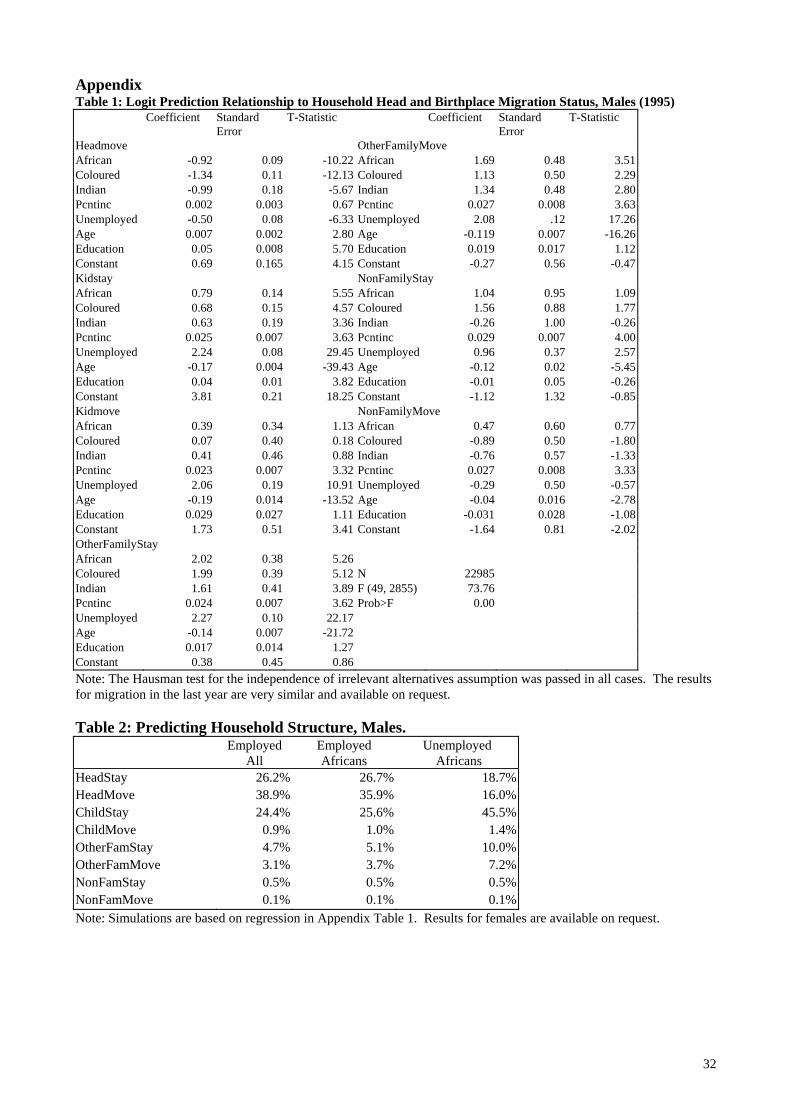
32
Appendix Table 1: Logit Prediction Relationship to Household Head and Birthplace Migration Status, Males (1995)
Coefficient Standard Error
T-Statistic Coefficient Standard Error
T-Statistic
Headmove OtherFamilyMove African -0.92 0.09 -10.22 African 1.69 0.48 3.51 Coloured -1.34 0.11 -12.13 Coloured 1.13 0.50 2.29 Indian -0.99 0.18 -5.67 Indian 1.34 0.48 2.80 Pcntinc 0.002 0.003 0.67 Pcntinc 0.027 0.008 3.63 Unemployed -0.50 0.08 -6.33 Unemployed 2.08 .12 17.26 Age 0.007 0.002 2.80 Age -0.119 0.007 -16.26 Education 0.05 0.008 5.70 Education 0.019 0.017 1.12 Constant 0.69 0.165 4.15 Constant -0.27 0.56 -0.47 Kidstay NonFamilyStay African 0.79 0.14 5.55 African 1.04 0.95 1.09 Coloured 0.68 0.15 4.57 Coloured 1.56 0.88 1.77 Indian 0.63 0.19 3.36 Indian -0.26 1.00 -0.26 Pcntinc 0.025 0.007 3.63 Pcntinc 0.029 0.007 4.00 Unemployed 2.24 0.08 29.45 Unemployed 0.96 0.37 2.57 Age -0.17 0.004 -39.43 Age -0.12 0.02 -5.45 Education 0.04 0.01 3.82 Education -0.01 0.05 -0.26 Constant 3.81 0.21 18.25 Constant -1.12 1.32 -0.85 Kidmove NonFamilyMove African 0.39 0.34 1.13 African 0.47 0.60 0.77 Coloured 0.07 0.40 0.18 Coloured -0.89 0.50 -1.80 Indian 0.41 0.46 0.88 Indian -0.76 0.57 -1.33 Pcntinc 0.023 0.007 3.32 Pcntinc 0.027 0.008 3.33 Unemployed 2.06 0.19 10.91 Unemployed -0.29 0.50 -0.57 Age -0.19 0.014 -13.52 Age -0.04 0.016 -2.78 Education 0.029 0.027 1.11 Education -0.031 0.028 -1.08 Constant 1.73 0.51 3.41 Constant -1.64 0.81 -2.02 OtherFamilyStay African 2.02 0.38 5.26 Coloured 1.99 0.39 5.12 N 22985 Indian 1.61 0.41 3.89 F (49, 2855) 73.76 Pcntinc 0.024 0.007 3.62 Prob>F 0.00 Unemployed 2.27 0.10 22.17 Age -0.14 0.007 -21.72 Education 0.017 0.014 1.27 Constant 0.38 0.45 0.86 Note: The Hausman test for the independence of irrelevant alternatives assumption was passed in all cases. The results for migration in the last year are very similar and available on request. Table 2: Predicting Household Structure, Males.
Employed All
Employed Africans
Unemployed Africans
HeadStay 26.2% 26.7% 18.7%HeadMove 38.9% 35.9% 16.0%ChildStay 24.4% 25.6% 45.5%ChildMove 0.9% 1.0% 1.4%OtherFamStay 4.7% 5.1% 10.0%OtherFamMove 3.1% 3.7% 7.2%NonFamStay 0.5% 0.5% 0.5%NonFamMove 0.1% 0.1% 0.1%Note: Simulations are based on regression in Appendix Table 1. Results for females are available on request.
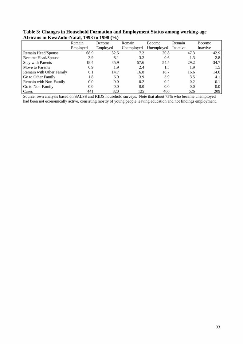
33
Table 3: Changes in Household Formation and Employment Status among working-age Africans in KwaZulu-Natal, 1993 to 1998 (%) Remain
Employed Become Employed
Remain Unemployed
Become Unemployed
Remain Inactive
Become Inactive
Remain Head/Spouse 68.9 32.5 7.2 20.8 47.3 42.9Become Head/Spouse 3.9 8.1 3.2 0.6 1.3 2.8Stay with Parents 18.4 35.9 57.6 54.5 29.2 34.7Move to Parents 0.9 1.9 2.4 1.3 1.9 1.5Remain with Other Family 6.1 14.7 16.8 18.7 16.6 14.0Go to Other Family 1.8 6.9 3.9 3.9 3.5 4.1Remain with Non-Family 0.0 0.0 0.2 0.2 0.2 0.1Go to Non-Family 0.0 0.0 0.0 0.0 0.0 0.0Cases 441 320 125 466 626 209Source: own analysis based on SALSS and KIDS household surveys. Note that about 75% who became unemployed had been not economically active, consisting mostly of young people leaving education and not findings employment.