survivor interaction contrast wiggle predictions of

Journal of Mathematical Psychology 58 (2014) 21–32

Contents lists available at ScienceDirect

Journal of Mathematical Psychology

journal homepage: www.elsevier.com/locate/jmp

Survivor interaction contrast wiggle predictions of parallel and serialmodels for an arbitrary number of processesHaiyuan Yang a,∗, Mario Fific b, James T. Townsend a

a Department of Psychological and Brain Sciences, Indiana University, Bloomington, IN, 47405, USAb Psychology Department, Grand Valley State University, MI, 49401, USA

h i g h l i g h t s

• We explore the precise behavior of the serial exhaustive SIC function for n = 2.• We provide a generalization of the SIC function to an arbitrary number of processes.• We analyze the generalized SIC for both parallel and serial models with minimum and maximum time stopping rules.• We demonstrate application of the theorems to data from a short-term memory search task.

a r t i c l e i n f o

Article history:

Keywords:Survivor interaction contrastHuman information processingLogarithmic concavityMulti-processes

a b s t r a c t

The Survivor Interaction Contrast (SIC) is a distribution-freemeasure for assessing the fundamental prop-erties of human information processing such as architecture (i.e., serial or parallel) and stopping rule(i.e., minimum time or maximum time). Despite its demonstrated utility, there are some vital gaps inour knowledge: first, the shape of the serial maximum time SIC is theoretically unclear, although the one0-crossing negative-to-positive signature has been found repeatedly in the simulations. Second, the the-ories of SIC have been restricted to two-process cases, which restrict the applications to a limited class ofmodels and data sets. In this paper, we first prove that in the two-process case, a mild condition known asstrictly log-concavity is sufficient as a guarantor of a single 0-crossing of the serial maximum time SIC.Wethen extend the definition of SIC to an arbitrary number of processes, and develop implicated methodol-ogy of SIC in its generalized form, again in a distribution-free manner, for both parallel and serial modelsin conjunction with both the minimum time and maximum time stopping rules. We conclude the paperby demonstrating application of the theorems to data from a short-term memory search task.

© 2013 Published by Elsevier Inc.

1. Introduction

The question of whether people can perform multiple percep-tual or mental operations simultaneously, that is, parallel process-ing, vs. whether items or tasks must proceed serially (one at atime), has intrigued psychologists since the birth of experimen-tal psychology. Historically, reaction time (RT) has been the pri-mary measure on this question. The work of the physiologist F.C.Donders (e.g., Donders, 1868) was seminal in this regard, althoughother researchers, such as W. Wundt, were more prolific with re-gard to early results on human cognition.

With the revolution brought about through cognitive scienceand cognitive psychology in the 1950s and 1960s, questions suchas the parallel vs. serial conundrum, which had lain dormant sincethe nineteenth century saw a renaissance of interest.

∗ Corresponding author.E-mail addresses: [email protected] (H. Yang), [email protected] (M. Fific),

[email protected] (J.T. Townsend).

0022-2496/$ – see front matter© 2013 Published by Elsevier Inc.http://dx.doi.org/10.1016/j.jmp.2013.12.001

The serial vs. parallel topic is our primary concern here. How-ever, it may be worth a moment’s pondering, given the pioneeringrole of William K. Estes in the advent of mathematical psychol-ogy, of how the latter field, and Estes’ research, fit into, and con-tributed to, modern cognitive psychology. Three tributaries fed thenew stream of mathematical psychology in the 1950s and 60s.These were: 1. Signal detection theory, child of psychophysics andsensory processes, mathematical communications theory, appliedphysics, and statistical decisionmaking (e.g., Green & Swets, 1966;Tanner & Swets, 1954). 2. Foundationalmeasurement the offspringof S.S. Stevens’ brilliant but non-rigorous statements concern-ing measurement in psychology fostered and rendered rigorousthrough strands from philosophy, mathematical logic and abstractalgebra (e.g., Krantz, Luce, Suppes, & Tversky, 1971; Roberts &Zinnes, 1963). 3. Mathematical learning theorywhichwent back atleast to Clark Hull (e.g., Hull, 1952); or see Koch’s elegant summaryin Modern Learning Theory (Koch, 1954). This branch is where wefind the Estes trailblazing Stimulus Sampling Theory (Estes, 1955,1959), a precise, quantitative theory of human and animal learning.

http://dx.doi.org/10.1016/j.jmp.2013.12.001

http://www.elsevier.com/locate/jmp

http://www.elsevier.com/locate/jmp

http://crossmark.crossref.org/dialog/?doi=10.1016/j.jmp.2013.12.001&domain=pdf

mailto:[email protected]



http://dx.doi.org/10.1016/j.jmp.2013.12.001

22 H. Yang et al. / Journal of Mathematical Psychology 58 (2014) 21–32

This theory,which still impacts awide spectrumof research in cog-nition today, led to a score of research advances by Estes and col-leagues as well as a host of other scientists (e.g., Atkinson & Estes,1963; Friedman et al., 1964).

Estes was an early entrant into the embryonic cognitive move-ment. His research in this domain was likely influenced by theburgeoning efforts utilizing the information processing approach,perhaps the early dominant theme in this new domain. Early pio-neers includedWendell Garner (e.g., Garner, 1962), Donald Broad-bent (e.g., Broadbent, 1958), William Hick (e.g. Hick, 1952), andColin Cherry (e.g. Cherry, 1953) (note the heavy presence of Britishpsychologists).

American psychologists were soon contributing to this rapidlyexpanding field which bridged sensory processes, higher percep-tion, and elementary cognition. Prime examples are Charles Erik-sen (e.g., Eriksen & Spencer, 1969), Michael Posner (e.g., Posner,1978), Raymond Nickerson (e.g., Nickerson, 1972), Ralph Haber(e.g., Haber & Hershenson, 1973), and Howard Egeth (e.g., Egeth,1966). And, Bill Estes of course.

The employment of ingenious experimental designs to answerquestions concerning whether humans perform visual or mem-ory search in a serial or parallel fashion provide apt examples ofnew trends making an appearance in the 60s and 70s. (e.g., Sper-ling, 1960, 1967; Sternberg, 1966, 1975). Estes and colleagues pro-vided some classic early results in this domain in extending, andmathematicallymodeling extensions of Sperlings innovative visualsearch experimental designs. For instance, Estes and Taylor (1964)developed a new detection method as well as associated modelsin this vein. Also, Estes and Taylor (1966) and Estes and Wessel(1966)were beginning to explore phenomena andhuman informa-tion processing mechanisms related to the presence of redundantsignals in visual displays.

The Sternberg (1966) innovative and rather startling RT data inshort termmemory search, in particular, had a profound influenceon thinking in the parallel vs. serial processing literature. In fact, amassive body of experimental literature over several decades hasbeen based on the inference that increasing, more-or-less straight-line RT functions of the workload n,1 the number of comparisonsto perform, imply serial processing. However, the ability of lim-ited capacity parallel models to mimic serial models, in the strongsense of mathematical equivalence, was demonstrated relativelyearly on (e.g., Atkinson, Holmgren, & Juola, 1969; Murdock, 1971;Townsend, 1969, 1971).2 And in fact, the reverse possibility of se-rial models to mimic parallel models was also proven (Townsend,1969, 1971, 1972, 1974). The early mathematical results were con-fined to limited types of RT distributions, but later developmentsextended to arbitrary probability distributions (Townsend, 1976;Townsend & Ashby, 1983; Vorberg, 1977).

The parallel models which perfectly mimic serial models arelimited capacity in the sense that their processes degrade in their ef-ficiency as the workload n increases. Suchmodels intuitively makethe predictions associated with serial processing, specifically thelinear RT graphs of the workload n (e.g., Townsend, 1971). Fortu-nately, theory-driven experimental methodologies have been in-vented in recent years that are considerably more robust in the

1 An increment in workload is usually natural to define in terms of number ofdimensions, or subtasks involved in some task. We shall often refer simply to itemsor, sometimes, processes as generic tags for the discrete objects being processed orthe conduits working on them. The unit of workload typically relates in a naturalfashion to the task. For example, if a memory search task involves examination of alist of letters, the unitmay bemade straightforwardly in terms of letters. Then nmaystand for both the workload in the task and the number of letters in the memoryset.2 For an up to date review of the parallel–serial identifiability issue, see

Townsend, Yang, and Burns (2011).

assessment of mental architecture, particularly serial vs. parallelprocessing (Scharff, Palmer, &Moore, 2011; Townsend, 1976, 1981,1990a; Townsend & Nozawa, 1995; Townsend &Wenger, 2004). Inparticular, the new methodologies often allow architectural infer-ences even though the workload is held constant, so that capacitydoes not confound architectural inferences.

Our focus here lies within the general approach referred to asSystems Factorial Technology (hereafter SFT; see Townsend, 1992;Townsend & Nozawa, 1995). A number of investigators have madeessential contributions to this literature including Schweickert andDzhafarov and colleagues (Dzhafarov, 1997; Dzhafarov, Schwe-ickert, & Sung, 2004; Schweickert, 1978, 1982; Schweickert &Giorgini, 1999; Schweickert, Giorgini, & Dzhafarov, 2000). SFT re-lies heavily onmathematical propositions indicating experimentalconditions where strong tests of architectures may be found, al-though other testable features, such as capacity, are also encom-passed presently. The bulk of theoretical work has been performedunder the assumption of selective influence. Our scope prohibits de-tails here, butwe can loosely define selective influence as the prop-erty that certain experimental factors act only on specific processesin the overall system (see Section 2.1 for more detailed discussionon selective influence). When selective influence is in force, pre-dictions of serial and parallel models and the pertinent decisionalstopping rules are strikingly distinct. This paper is intended to sig-nificantly strengthen and extend these predictions.

SFT requires the survivor function S(t), which is simply thecomplement of the well-known cumulative distribution (or fre-quency) function (the CDF) written as F(t). That is, S(t) = 1−F(t).A central statistical diagnostic is then the survivor interaction con-trast (or SIC) function. It performs a double difference contrast op-eration on the survivor functions that is analogous to the meaninteraction contrast (orMIC) employed on the arithmetic RTmeansin earlier investigations (e.g., Schweickert, 1978; Sternberg, 1966).However, it now expresses a highly diagnostic function of time,rather than a single number.

Despite the successful deployment of the SICmeasure, there aresome vital gaps in our knowledge, restricting the applications to alimited class ofmodels and data sets. Thesewill be sketchedwithina brief presentation of relevant knowledge we do have.

We know that, for n = 2, serial minimum time models predictperfectly flat signatures whereas serial maximum time (i.e., theclassical exhaustive processing time stopping rule; see Sternberg,1969; Townsend, 1974) predictions must include at least one wig-gle (i.e., the up-and-down excursions marked by 0-crossings) be-low and above 0 (Townsend & Nozawa, 1995). However, althoughsimulations have intimated that there is a single wiggle passingthrough 0, in a negative-to-positive direction as exhibited in Fig. 1(the top right panel), this has not been shown to be true for all dis-tributions. In fact, the exact shape of the SIC curve is as yet un-known.

Therefore, in elucidating further properties of serial exhaustiveprocessing: A. We first prove that serial exhaustive processing in-evitably predicts an odd number of 0-crossings in the n = 2 case.B. Next, we show that a certain readily-met mathematical condi-tion is sufficient to force the behavior indicated through our simu-lations, a single 0-crossing of the SIC function.

The behavior our SIC signatures have also remained unidenti-fied for n > 2, in the case of all studied serial and parallel processesup to now. The quite intriguing behaviors in the case of the serialand parallel models with varying stopping rules, and for arbitraryvalues of n, are next developed for: A. Serial minimum time pro-cessing. B. Serial maximum time processing. C. Parallel minimumtime processing. D. Parallel maximum time processing.

Successful completion of the above goals should significantlyexpand the possibilities of application. Since mathematical detailsof SFT in general, have been published elsewhere (e.g., Townsend &Nozawa, 1995) and tutorials are available (e.g., Townsend, Fific, &Neufeld, 2007; Townsend &Wenger, 2004; Townsend et al., 2011),only the bare bones SFT can be displayed here.

H. Yang et al. / Journal of Mathematical Psychology 58 (2014) 21–32 23

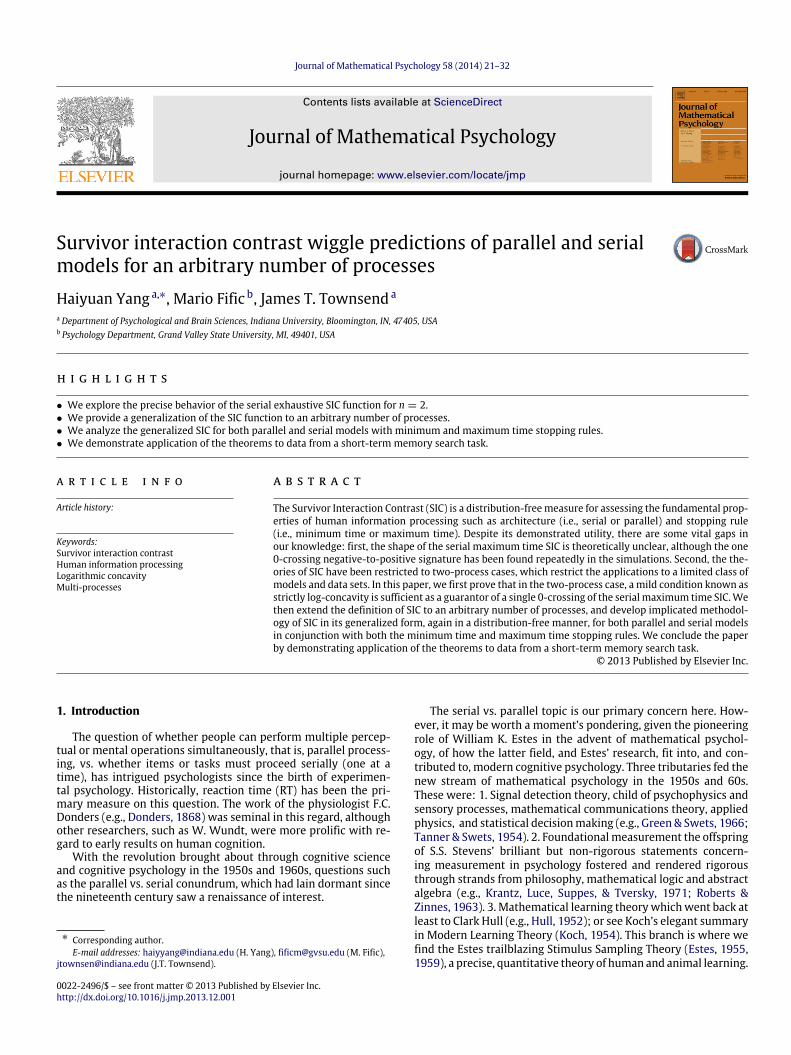
Fig. 1. Representative predictions of survivor interaction contrast (SIC) and mean interaction contrast (MIC) across different architectures and stopping rules. The fourcanonical models on the left are based on simulations of gamma distributions, with various shape parameters regarding different salience levels of processes. The coactivemodel on the right is based on simulations of dynamic systems described in (Townsend &Wenger, 2004).

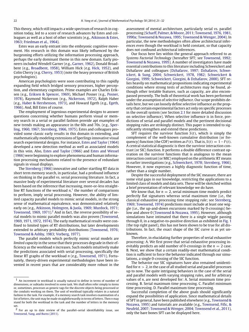
Fig. 2. Distributional influences of the high vs. low salience manipulation with survivor functions (right) and densities suggesting satisfaction of the one point crossover(left). The simulations are based on gamma distributions with different shape parameters.

2. Extending knowledge of serial exhaustive processing: analy-sis for two processes

2.1. Underlying assumptions of SFT

The critical assumption underlying SFT is selective influence,which means that an experimental factor affects only a single pro-cess. We continued the convention (Townsend & Ashby, 1983) ofindicating the level of a factor as high if it speeds up the process andas low when it slows down the process. Manipulating the speedof the process is also referred to as salience manipulation. In theshort-term memory search task shown in the exemplar experi-ment section, for instance, high dissimilarity between the item inthe memory and the target will be designated as a high saliencelevel, and low dissimilarity between item and target will be desig-nated as a low salience level.

In terms of RT distribution, an experimental variable acting se-lectively could in principle affect any one ormore of several aspectsof an RT distribution. In this paper we follow the assumption as ex-pressed in Townsend and Nozawa (1995) that the two processingtime density functions for a single process, at the two factor levelscross exactly once, i.e., there is exactly one time t∗, where the twodensity functions are equal. This assumption implies an orderingof both survivor functions (i.e. stochastic dominance) aswell as themeans andmedians. This assumption appears to be satisfiedwithinthe limits of typical psychological applications (e.g., Townsend,1990b; Townsend & Nozawa, 1995). Fig. 2 shows a hypotheticalexample of selective influence operating at the one-point density

crossover level, using two gammadistributed variables.We can seethat the property of single density crossover (left panel) leads toboth an ordering of the survivor functions (right panel) and of themean processing times (right panel, the area under the survivorcurves).

In order to avoid possible failure of selective influence due to in-direct non-selective influence, i.e., one factor can indirectly affectthe ‘wrong’ process through stochastic dependence (Townsend,1984; Townsend & Thomas, 1994), some condition concerningstochastic independence is typically required. For simplicity ofproof, stochastic independence of the process completion timesis assumed, although Dzhafarov (1999, 2003) and Dzhafarov et al.(2004) has shown that conditional independence given some com-mon sources of randomness which are unaffected by the experi-mental factors is sufficient for these purposes.3

Therefore, not onlymust selective influence act at a level of suf-ficient power on a process X (e.g., the density single point crossingassumption above), but itmust be assumed that themarginal prob-ability functions on processing times for all other processes Y , Z ,etc.must be invariantwhen the X factor ismanipulated. Base times(all else besides the completion times of the processes in whichweare interested) are avoided in this study but under the assumptionof conditional independence, would not affect our results in anyevent.

3 See Kujala and Dzhafarov (2008) for recent advances pertaining to selectiveinfluence.


2.2. Limited review of systems factorial technology

Suppose we are concerned with just two processes or channels.We refer to these as X and Y . Let fXL(t) be the density functionof the processing time on X when the factor level of process X islow and fXH(t) be the density function of the processing time on Xwhen the factor level is high. Likewise, let fYL(t) and fYH(t) be thedensity functions of the processing time on Y when the factor levelof Y is low and high, respectively. In this paper we assume that alldensity functions are sufficiently smooth.4 Let SXL(t), SXH(t), SYL(t)and SYH(t) denote the survivor functions corresponding to fXL(t),fXH(t), fYL(t) and fYH(t) respectively. A survivor function of randomvariable T is defined as

S(t) = P(T > t) =

∞

tf (t ′)dt ′ = 1 − F(t). (1)

The Survivor Interaction Contrast (SIC) function of the total re-action time T (later we use T with subscripts to denote reactiontimes of single process) is defined as

SIC2(t) = (SLL(t) − SLH(t)) − (SHL(t) − SHH(t)). (2)The superscript indicates the number of processes, and subscriptsare used to denote the salience level of each process. For exam-ple, SLL(t) indicates the survivor function of RT for the condition inwhich both process X and Y are of low salience. For simplicity, weuse∆2 to denote the double differences over the factor level, henceEq. (2) becomes SIC2(t) = ∆2

X,Y S(t). Theoretically, the observed RTshould be a combination of process completion times, with appro-priate forms (i.e. sum,max,min, or probabilitymixture) dependingon the underlying stopping rules.

Themean interaction contrast (MIC) is also an important statis-tic in distinguishing among certain processing types.With RT indi-cating themean response time and the subscripts as defined above,the MIC is given by

MIC = (RT LL − RT LH) − (RTHL − RTHH). (3)Sternberg (1969) suggested that based on selective influence,

serial models with independent processing times would exhibitMIC = 0. The use of MIC has later been extended to diagnoseparallel processing (Schweickert & Townsend, 1989; Townsend &Nozawa, 1995). The SIC and MIC predictions5 of the four standardmodels are shown in Fig. 1. Note that, due to the fact that the in-tegral of the survivor function of a positive random variable is itsexpected value, the interaction contrast of mean values is equal tothe integrated SIC, i.e.,

∞

0 SIC(t)dt = MIC.Fig. 1 shows that parallel-processing SICs reveal total positivity

(i.e. the SICs are non-negative functions of t) in the case of mini-mum time conditions (MIC > 0) but total negativity in the caseof maximum time conditions (MI < 0). On the other hand, serialminimum time SICs are equal to zero at all time values t (MIC =

0), while simulation results have repeatedly found, in contrast, thatserialmaximum time (or serial exhaustive) SICs show a large nega-tive portion, followed by an equally large positive portion (MIC =

0). The coactive model, based on the summed Poisson processes,predicts that the SIC is negative for small times and then positivefor later times, much like the SIC for the serial exhaustive model.But the negative region is always smaller than the positive region,which leads to a positive MIC value6 (MIC > 0). Thus each of

4 A smooth function of class Ck is a function that has continuous derivatives upto the kth order in its domain. Here the term ‘‘sufficiently smooth’’ means that thedensity functions do not need to be of class C∞ , but all operations on the densityfunctions mentioned in this paper should be well defined.5 For rigorous proofs of SIC predictions, see Townsend and Nozawa (1995);

Townsend and Wenger (2004).6 Although both coactive models and parallel race models predict everywhere-

positive OR MIC results, an investigator might test them using a result of

the five models makes a unique prediction for the combination ofMIC value and SIC shape. By using both the MIC and SIC statistics,one can differentiate between serial, parallel, and coactive archi-tectures, as well as minimum time and exhaustive stopping rules.

As observed earlier, for the case of serial exhaustive process-ing, Townsend andNozawa (1995) proved that the SIC function be-gins negative but must be positive for substantial values of t > 0.In fact, the summation of the positive portion of SICs is equal tothe summation of the negative portion, since the mean interactioncontrast must be zero. However, it does not follow from the exist-ing proofs that the SIC must be the 1-wiggle S-shape function asfound in the simulations of Fig. 1.

Can it be demonstrated that the 1-wiggle SIC behavior appliesto all distributions when convolved to produce serial exhaustivepredictions? This might seem rather unlikely given that, in prin-ciple the underlying distributions are arbitrary. Are there non-trivial conditions that are necessary and/or sufficient to elicit the1-wiggle portrait? In attempting to answer these questions, wehave first of all discovered novel aspects of generalwiggle behaviornot only for the involved processes of n = 2 but for arbitrary n ≥ 2.

We are now prepared for our first theoretical result.

2.3. Theoretical propositions

Although we know from previous work (Townsend & Nozawa,1995) thatwigglesmust exist for 2-stage serial exhaustive process-ing, we do not know howmany in general we should expect. Thenour first result demonstrates that for any underlying processingdistributions in series, the number of crossovers of 2-stage serialexhaustive SIC must be an odd number.7

Proposition 2.1. Assume selective influence. The independent serialexhaustive SICmust have an odd number of crossovers with horizontalaxis in the interval (0, +∞).

Proof. The overall RT in serial exhaustive models should be thesummation of the completion times of two processes X and Y ,i.e., T = TX + TY . Since we assume that two channels process in-dependently, we can write the survivor interaction contrast as

SIC2ser.AND(t) = ∆2

X,YP(TX + TY > t)

= −∆2X,Y

t

0FX (t − ty) × fY (ty)dty

= −

t

0

FXL(t − ty) × fYL(ty) − FXL(t − ty) × fYH(ty)

− FXH(t − ty) × fYL(ty) + FXH(t − ty) × fYH(ty)dty

= −

t

0

[FXH(t − ty) − FXL(t − ty)]

×[fYH(ty) − fYL(ty)]dty. (4)

Because of the action of selective influence on the survivor func-tions, the firstmultiplicand under the integral sign is non-negative.Further,when selective influence operates at the one-point densitycrossover level, the secondmultiplicandwill be positive for t < t∗,where t∗ represents the density crossover point. Thus SIC functionmust be negative for small times t < t∗.

To show that there are odd number crossovers, we need todemonstrate that when t → ∞, the SIC2(t) must converge to zero

Schweickert and Wang (1993). Namely, if the factor levels are increased over asufficiently large range, parallel race models predictions will approach a MIC limitwhereas coactive models predictions will not.7 In this paper, we restricted our discussion to finite-zero cases, i.e., the number

of crossovers of SIC would be either even or odd.


from the positive side. Let DFX (t) = FXH(t) − FXL(t), DfY (t) =

fYH(t) − fYL(t). Because of the property of commutativity of con-volution, we can rewrite SIC2(t) as

SIC2ser.AND(t) = −

t

0DFX (t − ty) × DfY (ty)dty

= −

t

0DFX (ty) × DfY (t − ty)dty. (5)

Denote I2(s) = s0 SIC2

ser.AND(t)dt . By Fubini’s theorem,

I2(s) = −

s

0

t

0DFX (ty) × DfY (t − ty)dtydt

(Change the order of integration)

= −

s

0

s

tyDFX (ty) × DfY (t − ty)dtdty

(Definition of density function)

= −

s

0DFX (ty) × DFY (s − ty)dty. (6)

Because of the action of selective influence on the survivor func-tions, both DFX (t) and DFY (t) are positive, thus I2(s) is negative.Another fact about I2(s) is that it goes to zero when s → ∞ (re-call that I2(∞) = MIC). Combining these two facts together wesee that I2(s) must increase toward zero from the negative side atthe end. Thus the derivative of I2(s), i.e. SIC2(s), must be positiveas long as s is large enough.

Having shown that the SIC function is negative for small timevalues and positive when it approaches to zero at the end, the im-plication is that the SIC must have an odd number of crossovers in(0, +∞). �

Many simulations with differing distributions have intimatedthat perhaps the odd number of crossovers might typically just be1. It is next proven that a satisfyingly weak condition ensures thatthiswill be the case. However, first a brief discussion of the relevanthistory is in order.

From Eq. (5) we see that the serial exhaustive SIC curve is a con-volution of the difference in probability density functions, of thehigh salience minus the low salience on the X factor, and the dif-ference in cumulative distribution functions of the high salienceminus the low salience on the Y factor. Further, the integral of theSIC2(t) with variable upper limit, i.e., I2(s), is also a convolution,of two functions which are the two differences in cumulative dis-tribution functions on X and Y factor respectively. For many years,it was thought that a condition of unimodality8 of such functionswas enough to produce our needed result of a single 0-crossing.This was eventually found to be false. That is, it can be shown thatunimodality of both functions in the convolution is not sufficient toimply unimodality of the integral (Chung, 1953). In contrast, Ibrag-imov (1956) proposed and demonstrated that the convolution ofany two unimodal functions will be still unimodal, if at least one ofthem is logarithmic concave (so called strong unimodal).9

Proposition 2.2. Assume selective influence. The independent serialexhaustive SIC crosses the time axis only once in the interval (0, +∞),if either FXH(t) − FXL(t) or FYH(t) − FYL(t) is strictly log-concave.

8 Different sources have slightly different definitions for a unimodal function.Weshall use the following: a mode of a function f is a number a such that (a). f is non-decreasing on (−∞, a] and (b). f is non-increasing on [a, ∞). f is unimodal if it hasa mode. f is strictly unimodal if it has a single mode.9 ‘‘Concavity’’ of an increasing curvemeans that it bends downward as it ascends,

implying a so-called ‘‘negative second derivative’’ in elementary calculus. ‘‘Log-concavity’’ then simply means that the logarithm of the function rather than thefunction itself is concave.

Proof. Let DFX (t) = FXH(t)− FXL(t), DFY (t) = FYH(t)− FYL(t). Alsolet DfX (t) = fXH(t) − fXL(t), DfY (t) = fYH(t) − fYL(t). Assume thatthe two processing time density functions at the two factor levels(fXL(t) and fXH(t); fYL(t) and fYH(t)) cross exactly once, thus bothDFX (t) and DFY (t) are strictly unimodal. Suppose DFY (t) is strictlylog-concave. Assume also, for themoment, thatDFY (t) has support(−∞, ∞), i.e., DFY (t) = 0 for all t ∈ (−∞, ∞) (we will removethis assumption later). We show that the SIC2(t) has only one 0-crossing for any DFX (t). This proof is based on Chapter 1 of Dhar-madhikari and Joag-Dev (1988).

Since convolution commutes with translations, we assume,without loss of generality, that DFX (t) is unimodal about 0, i.e.,DfX (t) > 0 for t < 0 and DfX (t) < 0 for t > 0. Recall from Eq. (5)that SIC2

ser.AND(t) = −

∞

−∞DfX (ty) × DFY (t − ty)dty. Then for any

t , z such that t < z, we have

SIC2ser.AND(z) = −

∞

−∞

DfX (ty)DFY (z − ty)DFY (t − ty)

× DFY (t − ty)dty. (7)

Since DFY (t) is strictly log-concave, DFY (t + δ)/DFY (t) is de-creasing in t if δ > 0 and increasing in t if δ < 0. Therefore,

DFY (z − ty)DFY (t − ty)

<DFY (z)DFY (t)

if ty < 0

and

DFY (z − ty)DFY (t − ty)

>DFY (z)DFY (t)

if ty > 0. (8)

But we also know that DfX (t) > 0 for t < 0 and DfX (t) < 0 fort > 0. Consequently Eq. (7) shows that

SIC2ser.AND(z) > −

DFY (z)DFY (t)

∞

−∞

DfX (ty)DFY (t − ty)dty

=DFY (z)DFY (t)

× SIC2ser.AND(t). (9)

Thus SIC2ser.AND(t) = 0 ⇒ SIC2

ser.AND(z) > 0 for all z > t .Therefore, SIC has only one 0-crossing and correspondingly, I2(s)is strictly unimodal.

The condition that DFY (t) is never zero can be removed by con-structing a series of strictly log-concave functions DF (m)

Y (t) that allhave support (−∞, ∞) and converge to DFY (t).10 Thus I2(m)(s) =

− s0 DFX (ty) × DF (m)

Y (s − ty)dty is strictly unimodal by the aboveproof. Since the class of strictly unimodal distributions on R isclosed under weak limits (Dharmadhikari & Joag-Dev, 1988, page3), let m → ∞, I2(s) is strictly unimodal,11 and SIC2(s) has onlyone 0-crossing. �

We should notice that Proposition 2.2 provides a sufficient butnot necessary condition for the single 0-crossing property of theSIC function. Hence even when both DFX (t) and DFY (t) are notstrictly log-concave, it is possible that the SIC function still hasonly one 0-crossing point. Does this result mean that the ‘‘log-concavity’’ condition is too far from necessary regarding this prob-lem? The answer is no. As indicated in Ibragimov (1956), for anyunimodal function that is not log-concave, there exists anotherunimodal function such that the convolution of the two functions ismulti-modal. In otherwords, for anyDFX (t) that is not log-concave,we can find a DFY (t) such that the corresponding SIC function hasmore than one zero.

10 For readerswho are interested in the details,we recommemd (Dharmadhikari &Joag-Dev, 1988), page 21, in which they show how to approximate the log-concavefunction g supported in [a, b] by the sequence g(m) supported in (−∞, ∞).11 Although (Dharmadhikari & Joag-Dev, 1988) demonstrated their theorem withdistributions, we can easily apply their result to our functions by rescaling I2(m)(s).


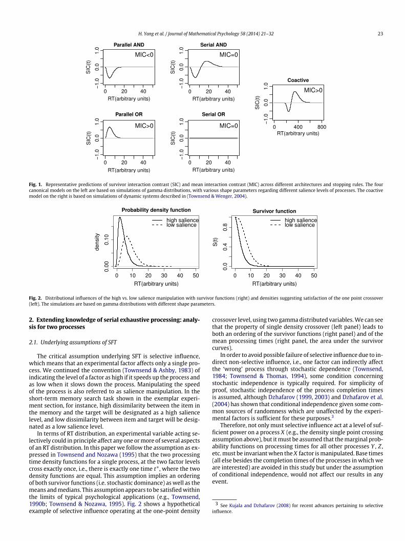
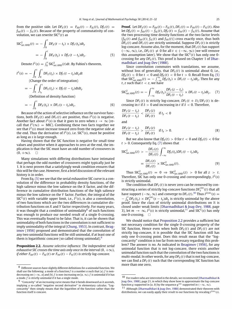
Fig. 3. An example of 2-stage serial exhaustive SIC function that has three 0-crossing points. Graphs include the density functions (top left), the difference of the twocorresponding survivor functions (top right), the SIC function (bottom left), and the integral of the SIC function with variable upper limits (bottom right).

We demonstrated the existence of multi-zero SICs by simula-tions. Completion times on processes were generated for both lowand high salience regarding the following rules: 1. For simplicity,we let completion times on processes X and Y have the same dis-tribution form, i.e., FXL(t) = FYL(t), FXH(t) = FYH(t). Thus DFX (t) =

DFY (t). 2. The completion times under the two salience conditionsare both mixtures of uniform and Gaussian distributions with dif-ferent parameters designed so that the two density functions at thetwo factor levels cross exactly once and the corresponding DF(t) isunimodal (but not log-concave). The simulation results are shownin Fig. 3. The top panel shows the two density functions for the lowand high conditions on the left and the DF(t) on the right. The bot-tom left panel shows the SIC function calculated by taking the dou-ble differences of survivor functions from the top left panel, and thebottom right panel shows the result of the convolution of −DFX (t)andDFY (t), which is also the integral of the SIC function, aswe indi-cated in the proof above. Aswe predicted, the convolution functionin the bottom right has three (rather than one) turning points, andcorrespondingwith this is that the SIC function on the left has three0-crossing points. Also note that in the limit, the convolution func-tion in the bottom right equals 0 as it should, indicating the MIC isstill 0 as it should be due to seriality. This simulation supports ourfinding that when losing the property of log-concavity, the serialexhaustive SIC function may exhibit three non-trivial zeros.

It was intimated in the previous section that the condition oflog-concavity is not very restrictive. This claim is supported by con-sidering a simple power function (such as assumed in S.S. Steven’sfamous law): y = AxB, where A and B are positive constants, x is theindependent, and y the dependent variable. For B ≥ 2, this functionis positively accelerated, that is, is convex with the accelerationincreasing with B. Yet, however large B may be, it is always log-concave, since log(y) = log(A) + B × log(x) which is always con-cave. And as observed, many commonly used distributions obeythis caveat, such as the normal distribution, the exponential distri-bution, and the gamma distribution with shape parameter P ≥ 1,etc. Proposition 2.2 therefore strongly suggests that we should notbe astonished to discover a single 0-crossing when processing isserial with an exhaustive stopping rule.

Nonetheless, as mentioned earlier, the SIC has so far been re-stricted to the n = 2 case. This fact is of more than simple techni-cal interest, since it has excluded the methodology from the largernumbers of items or processes which are often used in perceptualand cognitive experiments. The next part of this paper is devoted togeneralizing the knowledge base of the SIC signatures to arbitraryvalues of n.

3. Fundamental architectural signatures for an arbitrary num-ber of processes

How the two basic architectures, parallel and serial with vary-ing stopping rules behave for n > 2 processes will be explored inthis section. Before digging into the detail of the extended theory,we first introduce a measure, which is analogous to the SIC2(t) inEq. (2), but in a more general form. It will be evident that the com-plete factorial design can be erected by a recursive embedding inhigher and higher values of n, as indicated when n = 3. The SICfunction of total reaction time T in 3-process case produces the ex-pressionSIC3(t) = [(SLLL(t) − SLLH(t)) − (SLHL(t) − SLHH(t))]

−[(SHLL(t) − SHLH(t)) − (SHHL(t) − SHHH(t))] (10)where superscript indicates the number of processes and sub-scripts are used to denote the salience level of each process. Forexample, SLLL(t) indicates the survivor function of RT for the con-dition inwhich all three processes are of low salience. Note that thefactorial combination of three factors with their two salience lev-els leads to eight experimental conditions, thus the SIC function in3-process case is composed of eight items. An abstract formwhichis equivalent to Eq. (10) is as follows: SIC3(t) = ∆3

X1,X2,X3S(t),

where Xi represents the process i. This form of SIC function can bestraightforwardly generalized to the case for arbitrary n processes:let us denote the individual process as Xi, i = 1, 2, . . . , n, thus theSIC function in the n-process case could be written as

SICn(t) = ∆nX1,...,XnS(t) (11)

in which ∆nX1,...,Xn

represents the n-order mixed partial differenceover the factor levels. Analogous to the 3-process SIC which con-tains 23 items, the n-process SIC function is composed of 2n sur-vivor functions.

Now we are ready to present the theoretical results for n > 2.Our goal is to demonstrate that for the two major stopping rules,minimumandmaximumprocessing times, the results for arbitraryn are close relatives to those for n = 2 in the case for both paralleland serial systems.12 Here we employ mathematical induction inthe proofs.Mathematical induction is usually used to establish thata given statement is true for all non-negative integers. It could bedone by proving that the first statement in the infinite sequence

12 We limit our scope on pure serial and parallel systems. Mixed system of serialand parallel is not addressed in this paper.


of statements is true, and then proving that if the first N (anyarbitrarily chosen number) statements in the infinite sequence ofthe statements are true, then so is the next one.

We begin with the basic parallel horse race—independent par-allel processing and a minimum time stopping rule.

3.1. Parallel minimum time processing

In the case for n = 2, the SIC is always positive. Proposition 3.1reveals that this is the canonical signature for all n.

Proposition 3.1. Assume selective influence. The independent paral-lel minimum time processing predicts that the SIC curve will alwaysbe positive as a function of time t, for every n.

Proof. Recall that without the consideration of base time, the to-tal reaction time in parallel minimum time process models shouldbe the minimum of the reaction time on each process i.e, T =

min(TX1, . . . , TXn). Since we assume that two channels process in-dependently, we have

SICnpar.OR(t) = ∆n

X1,...,XnP(min(TX1, . . . , TXn) > t)

= ∆nX1,...,Xn [P(TX1 > t) × · · · × P(TXn > t)]

(factoring)

= [P(TXnL > t) − P(TXnH > t)]

× ∆n−1X1,...,Xn−1

[P(TX1 > t) × · · · × P(TX(n−1) > t)]

= [FnH(t) − FnL(t)] × SICn−1par.OR(t) (12)

where subscripts are used to denote the salience level of each pro-cess. For example, TXnL indicates the RT for the condition in whichthe nth process is of low salience, FnL indicates the correspond-ing marginal CDF. Because of the action of selective influence onthe survivor functions, FnH(t) > FnL(t) for all t . Since SIC2

par.OR(t)is always positive (Townsend & Nozawa, 1995), we can inferthat SICn

par.OR(t) is always positive, by simple mathematical induc-tion. �

It is interesting that the sign of the parallel horse race SIC func-tion is always positive as n is varied. We will learn that this doesnot inevitably occur in a parallel system when considering differ-ent stopping rules. The next proposition treatsmaximum time par-allel processing.

3.2. Parallel maximum time processing

When n = 2, the SIC function is always negative. From theabove proposition with minimum time processing we might ex-pect an analogous invariance with a maximum time (i.e., exhaus-tive processing) stopping rule. Intriguingly, this expectation is notfulfilled as the following proposition reveals.

Proposition 3.2. Assume selective influence. The independent paral-lel exhaustive processing predicts underadditivity in the survivor func-tion when an even number of channels are processed, and predictsoveradditivity when an odd number of channels are processed.

Proof. Without the consideration of base time, the total reactiontime in parallel exhaustive process models should be the maxi-mum of the reaction time on each process, i.e., T = max(TX1, . . . ,TXn). Thus, we have

SICnpar.AND(t) = ∆n

X1,...,XnP(max(TX1, . . . , TXn) > t)

= ∆nX1,...,Xn [1 − P(max(TX1, . . . , TXn) 6 t)]

= −∆nX1,...,XnP(max(TX1, . . . , TXn) 6 t)

= −∆nX1,...,Xn [P(TX1 6 t) × · · · × P(TXn 6 t)]

(factoring)

= −[P(TXnL 6 t) − P(TXnH 6 t)]

× ∆n−1X1,...,Xn−1

[P(TX1 6 t) × · · · × P(TX(n−1) 6 t)]

= [FnL(t) − FnH(t)] × SICn−1par.AND(t). (13)

Because of the action of selective influence on the CDF, FnL(t) <FnH(t) for all t . As we know that SIC2

par.AND(t) is negative, we caninfer that SICn

par.AND(t) is negative when n is even and is positivewhen n is odd. �

This flip-flopping of the SIC function according to whether n isodd or even, and only for the exhaustive stopping rule, is quite sur-prising and should be highly useful in identifying mental architec-tures.

We next resume our investigation of serial systems with thesame two stopping rules; minimum time first.

3.3. Serial minimum time processing

Recall that in the case of serial processing, a minimum timestopping rule is simplicity itself — the very first completion bringsprocessing to a halt. This simplicity, reinforced with selective in-fluence, extracts a strong result.

Proposition 3.3. Assume selective influence. The independent serialminimum time processing predicts that the SIC will always be zero asa function of time t, for every n.

Proof. The total reaction time in serial minimum time processmodels should be the reaction time of the process chosen to be thefirst one processed. Let pi denote the probability of processing theith item first. Then the survivor function on the total reaction timecan be expressed as

S(t) = P(T > t)

=

ni=1

P(T > t|T = TXi) × P(T = TXi)

=

ni=1

pi × P(TXi > t). (14)

Due to the complete factorial design, the n-process SIC function iscomposed of 2n survivor functions, and all items will cancel eachother out in the ensuing contrast function. Thus, the minimumtime stopping rule leads immediately to a decisive, and invariantprediction. �

3.4. Serial maximum time processing

One of the most intriguing architectural signatures of the SICcurvewhen n = 2 is that of serial exhaustive processing, exhibitingas it does the presence of wiggles above and below zero. Aswe would expect, for arbitrary n, the mean interaction contrastfor a serial process with an exhaustive stopping rule must be 0due to the additivity of the processing times along with selectiveinfluence. The following proposition confirms this result usingsurvivor functions but it also follows almost immediately from theforegoing statement.

Proposition 3.4. Assume selective influence. The independent serialexhaustive processing predicts that the integral of the SIC function isalways equal to zero, for every n.

Proof. Without the consideration of base time, the total reactiontime in serial exhaustive process models should be the sum of thereaction time on each process, i.e., T = TX1 + · · · + TXn. We reveal


the relationship between the n-stage SIC function and the (n− 1)-stage SIC function as below

SICnser.AND(t) = ∆n

X1,...,XnP(TX1 + · · · + TXn > t)

= −∆nX1,...,XnP(TX1 + · · · + TXn 6 t)

= −∆nX1,...,Xn

t

0[fn(tn)

× P(TX1 + · · · + TX(n−1) 6 t − tn)]dtn

= −

t

0∆n

X1,...,Xn

[fn(tn)

× P(TX1 + · · · + TX(n−1) 6 t − tn)]dtn

(factoring)

= −

t

0

[fnL(tn) − fnH(tn)]

×[∆n−1X1,...,Xn−1

P(TX1 + · · · + TX(n−1) 6 t − tn)]dtn

= −

t

0

[fnH(tn) − fnL(tn)]

× SICn−1ser.AND(t − tn)

dtn. (15)

Notice that SICnser.AND(t) is a convolution. By Fubini’s theorem, the

integral of the convolution of two functions on the whole space issimply obtained as the product of the integrals of each function,thus the integral of the SIC function on the whole space could berewritten as

∞

0SICn

ser.AND(t)dt = −

∞

0

t

0[fnH(tn) − fnL(tn)]

× SICn−1ser.AND(t − tn)dtn

dt

= −

∞

0[fnH(t) − fnL(t)]dt

×

∞

0SICn−1

ser.AND(t)dt. (16)

Since both fnH(t) and fnL(t) are density functions, the first integralof the above equation is always zero. Thus for every n, the integralof the SIC function of serial exhaustive model is predicted to bezero. �

The next proposition indicates that the SIC function will flipover when the number of processes changes from even to odd andvice versa.

Proposition 3.5. Assume selective influence. The independent serialexhaustive processing predicts that the SIC function must be negativefor small times if n is even, and it must be positive for small times if nis odd.

Proof. It is easy to confirm this statement when we examinethe relationship between SICn

ser.AND(t) and SICn−1ser.AND(t) shown in

Eq. (15). Notice that the difference between the two density func-tions should be positive for small t because of selective influenceat the density crossing level. Thus, when t is small, SICn

ser.AND(t) andSICn−1

ser.AND(t) have different signs, because of the negative sign be-fore the integral in the above equation. �

Propositions 3.4 and 3.5 provide us some key properties of theSIC functions for serial exhaustive models, from which we garnersome idea about how the SIC signatures behave, and how they as-sist in identification of the architectures and stopping rules. Withregard to the further analysis of SIC curves, recall that in the previ-ous section, we discovered that in the n = 2 case, a mild assump-tion of log-concavity guarantees that there is only a single wigglethrough zero. Thus an intriguing question asks how many zerosthere will be in SICn

ser.AND(t)? Is there any trend we can discover asn increases? The following discussion shows that the answer to allthese questions depends on the analytic character of the function.For functions of certain form, the zeros of SICn

ser.AND(t)will increaseby 1 as n increases by 1.

Next, it may be remembered that in the previous sectionwe de-termined the zeros of SIC2

ser.AND(t) via the shape of its integral. Here,we again explore the integral of SICn

ser.AND(t) for the same purpose.Let In(s) denote the integral of SICn

ser.AND(t) with variable upperlimit. Eq. (17) reveals the relationship between In(s) and In−1(s),which eventually has the same convolution form as the relation-ship between SICn

ser.AND(t) and SICn−1ser.AND(t).

In(s) = −

s

0

t

0[fnH(tn) − fnL(tn)] × SICn−1

ser.AND(t − tn)dtn

dt

(Change the order of integration)

= −

s

0

s

tn[fnH(tn) − fnL(tn)] × SICn−1

ser.AND(t − tn)dt

dtn

= −

s

0

[fnH(tn) − fnL(tn)] ×

s

tnSICn−1

ser.AND(t − tn)dt

dtn

= −

s

0

[fnH(tn) − fnL(tn)] × In−1(s − tn)

dtn. (17)

Recall that with the assumption of log-concavity, I2(s) is a uni-modal function. So following the proof in Proposition 2.2, we as-sert that I3(s) is a one-wiggle S-shape function, just as SIC2

ser.AND(t),if FX3H(t) − FX3L(t) is strictly log-concave. More generally, withthe assumption of strictly log-concavity of DFXi, we can infer thatIn(s) should have the same key signature as SICn−1

ser.AND(t) by sim-ple math induction. Now the problem of convolution converts tothe operation of taking the derivative, that is, how the number of0-crossings change from SICn−1

ser.AND(t) to SICnser.AND(t) converts to

the question of how that number changeswhenwe take thederiva-tive of In(s). Unfortunately, there appears to be no uniform answerfor that question. In fact, for some particular functions such as theGaussian density function the outcome is pleasant since the nthderivative would have n zeros, which leads to the result that zerosof SICn

ser.AND(t) will increase by 1 as n increases by 1.However, in the general case, the question of the number of

zeros of the derivatives could be a quite complicated issue due tothe flexible forms of the distributions. As a result, although ourhypothesis that zeros would increase by 1 as n increases has beenobserved in simulations, theoretical analysis suggests that thishypothesis could be violated, especially when n is a large number.

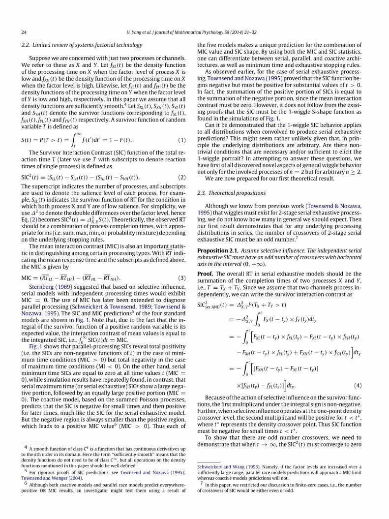
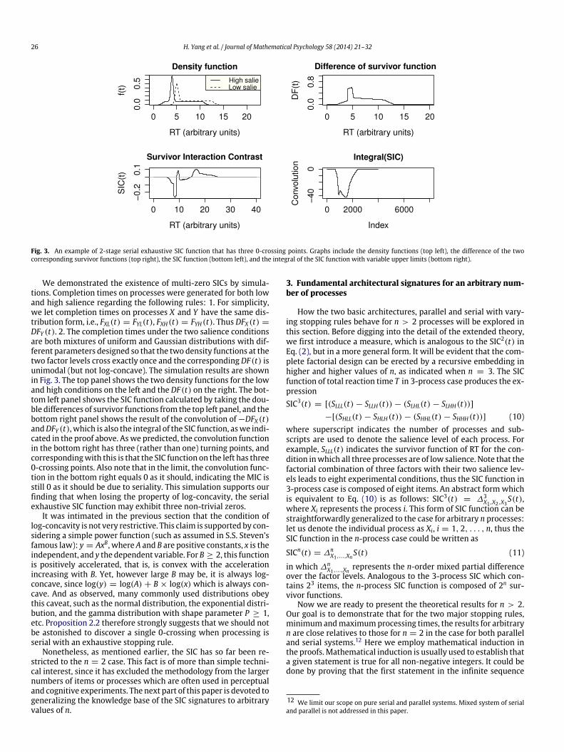
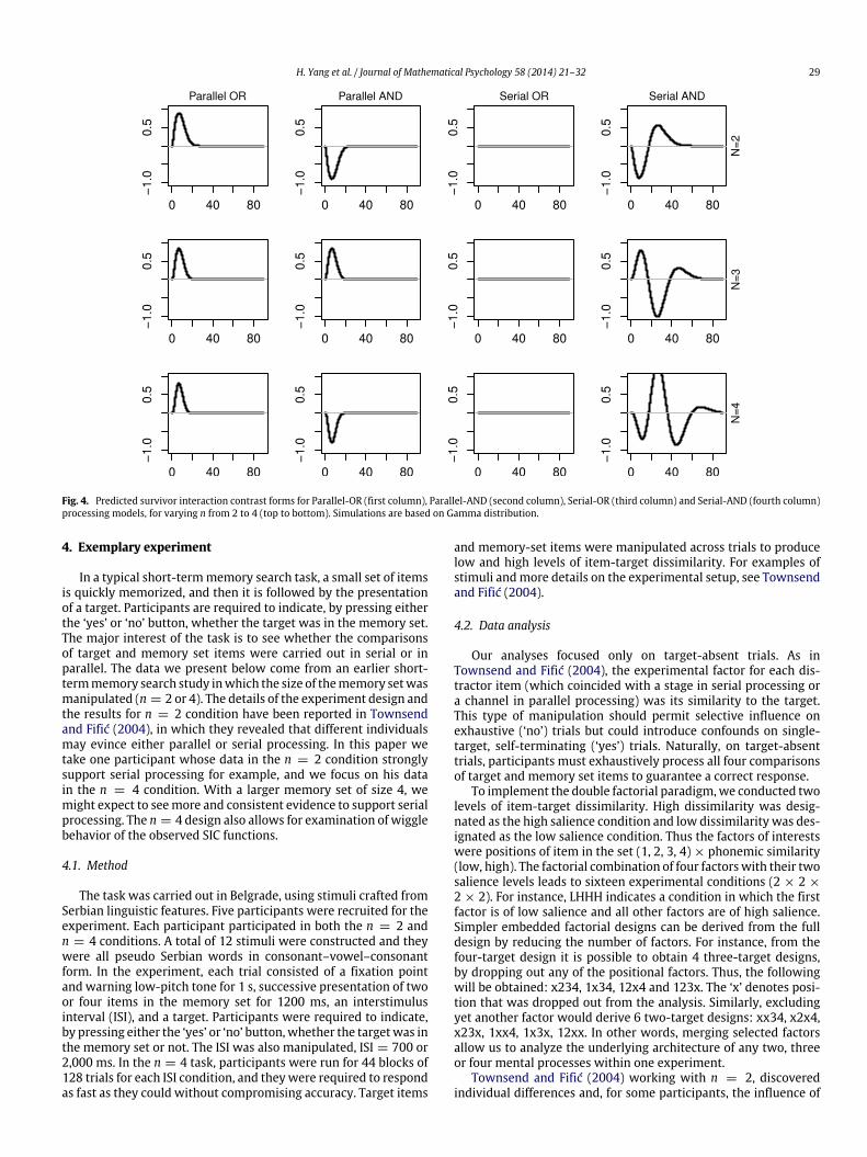
Fig. 4 exhibits simulation results which document the key sig-natures of the varying SIC functions. Briefly, Fig. 4 first depicted thefact that parallel minimum time processing models always predictan entirely positive SIC function (first column). Secondly, the curi-ous flip flopping of the parallel exhaustive systems from positiveto negative as n goes from odd to even is shown in the second col-umn. Thirdly, the absolute invariance of the minimum time serialprocessingmodels’ prediction that the entire curve is identical to 0appears in the third column of panels. Finally, the fascinating mul-tiplying of the wiggles in the serial exhaustive systems as n growsis illustrated in the fourth column of Fig. 4.


Fig. 4. Predicted survivor interaction contrast forms for Parallel-OR (first column), Parallel-AND (second column), Serial-OR (third column) and Serial-AND (fourth column)processing models, for varying n from 2 to 4 (top to bottom). Simulations are based on Gamma distribution.

4. Exemplary experiment

In a typical short-termmemory search task, a small set of itemsis quickly memorized, and then it is followed by the presentationof a target. Participants are required to indicate, by pressing eitherthe ‘yes’ or ‘no’ button, whether the target was in the memory set.The major interest of the task is to see whether the comparisonsof target and memory set items were carried out in serial or inparallel. The data we present below come from an earlier short-termmemory search study inwhich the size of thememory setwasmanipulated (n = 2 or 4). The details of the experiment design andthe results for n = 2 condition have been reported in Townsendand Fifić (2004), in which they revealed that different individualsmay evince either parallel or serial processing. In this paper wetake one participant whose data in the n = 2 condition stronglysupport serial processing for example, and we focus on his datain the n = 4 condition. With a larger memory set of size 4, wemight expect to seemore and consistent evidence to support serialprocessing. The n = 4 design also allows for examination of wigglebehavior of the observed SIC functions.

4.1. Method

The task was carried out in Belgrade, using stimuli crafted fromSerbian linguistic features. Five participants were recruited for theexperiment. Each participant participated in both the n = 2 andn = 4 conditions. A total of 12 stimuli were constructed and theywere all pseudo Serbian words in consonant–vowel–consonantform. In the experiment, each trial consisted of a fixation pointand warning low-pitch tone for 1 s, successive presentation of twoor four items in the memory set for 1200 ms, an interstimulusinterval (ISI), and a target. Participants were required to indicate,by pressing either the ‘yes’ or ‘no’ button,whether the targetwas inthe memory set or not. The ISI was also manipulated, ISI = 700 or2,000 ms. In the n = 4 task, participants were run for 44 blocks of128 trials for each ISI condition, and theywere required to respondas fast as they could without compromising accuracy. Target items

and memory-set items were manipulated across trials to producelow and high levels of item-target dissimilarity. For examples ofstimuli andmore details on the experimental setup, see Townsendand Fifić (2004).

4.2. Data analysis

Our analyses focused only on target-absent trials. As inTownsend and Fifić (2004), the experimental factor for each dis-tractor item (which coincided with a stage in serial processing ora channel in parallel processing) was its similarity to the target.This type of manipulation should permit selective influence onexhaustive (‘no’) trials but could introduce confounds on single-target, self-terminating (‘yes’) trials. Naturally, on target-absenttrials, participants must exhaustively process all four comparisonsof target and memory set items to guarantee a correct response.

To implement the double factorial paradigm,we conducted twolevels of item-target dissimilarity. High dissimilarity was desig-nated as the high salience condition and low dissimilarity was des-ignated as the low salience condition. Thus the factors of interestswere positions of item in the set (1, 2, 3, 4) × phonemic similarity(low, high). The factorial combination of four factorswith their twosalience levels leads to sixteen experimental conditions (2 × 2 ×

2 × 2). For instance, LHHH indicates a condition in which the firstfactor is of low salience and all other factors are of high salience.Simpler embedded factorial designs can be derived from the fulldesign by reducing the number of factors. For instance, from thefour-target design it is possible to obtain 4 three-target designs,by dropping out any of the positional factors. Thus, the followingwill be obtained: x234, 1x34, 12x4 and 123x. The ‘x’ denotes posi-tion that was dropped out from the analysis. Similarly, excludingyet another factor would derive 6 two-target designs: xx34, x2x4,x23x, 1xx4, 1x3x, 12xx. In other words, merging selected factorsallow us to analyze the underlying architecture of any two, threeor four mental processes within one experiment.

Townsend and Fifić (2004) working with n = 2, discoveredindividual differences and, for some participants, the influence of


Table 1Results of the Kolmogorov–Smirnov test applied to the full task.

hhhh lhhh hlhh hhlh hhhl llhh lhlh lhhl hllh hlhl hhll lllh llhl lhll hlll llll

hhhh >∗∗∗ >∗∗∗ >∗∗∗ >∗∗∗ >∗∗∗ >∗∗∗ >∗∗∗ >∗∗∗ >∗∗∗ >∗∗∗ >∗∗∗ >∗∗∗ >∗∗∗ >∗∗∗ >∗∗∗

lhhh − >∗∗∗ >∗∗∗ >∗∗∗ >∗∗∗ >∗∗∗ >∗∗∗ >∗∗∗ >∗∗∗ >∗∗∗ >∗∗∗ >∗∗∗

hlhh − >∗∗∗ >∗∗∗ >∗∗∗ >∗∗∗ >∗∗∗ >∗∗∗ >∗∗∗ >∗∗∗ >∗∗∗ >∗∗∗ >∗∗∗

hhlh − >∗∗∗ >∗∗∗ >∗∗∗ >∗∗∗ >∗∗∗ >∗∗∗ >∗∗∗ >∗∗∗ >∗∗∗ >∗∗∗ >∗∗∗

hhhl − >∗∗∗ >∗∗∗ >∗∗∗ >∗∗∗ >∗∗∗ >∗∗∗ >∗∗∗ >∗∗∗ >∗∗∗ >∗∗∗ >∗∗∗

llhh − − − − − >∗∗∗ >∗∗∗ >∗∗∗ >∗∗∗ >∗∗∗

lhlh − − − − − >∗∗∗ >∗∗∗ >∗∗ >∗∗∗ >∗∗∗

lhhl − − − − − >∗∗∗ >∗∗∗ >∗∗∗ >∗∗∗ >∗∗∗

hllh − − − − − >∗∗∗ >∗∗∗ >∗∗ >∗∗∗ >∗∗∗

hlhl − − − − − >∗∗∗ >∗∗∗ >∗∗∗ >∗∗∗ >∗∗∗

hhll − − − − − >∗∗∗ >∗∗∗ >∗∗∗ >∗∗∗ >∗∗∗

lllh − − − − − − − − − − − >∗∗∗

llhl − − − − − − − − − − − >∗∗∗

lhll − − − − − − − − − − − >∗∗∗

hlll − − − − − − − − − − − >∗∗∗

llll − − − − − − − − − − − − − − −

∗p < 0.1; ∗∗p < 0.05; ∗∗∗p < 0.01>∗∗∗: max(FHHHH (t) − FLHHH (t)) is significant, p < 0.01, etc.−: max(FLHHH (t) − FHHHH (t)) is not significant, etc.

the ISI betweenmemory-set presentation and the probe. However,all the SIC functions decisively adhered to either a serial or paral-lel form. To demonstrate the use of the new theories for revealingarchitecture for multiple processes, we take one participant (Par-ticipant 1 in Townsend and Fifić (2004)) whose data consistentlysupport serial processing as an example of our new theoretical re-sults. We were therefore curious to examine behavior for largern, particularly since most memory search experiments are basedon n > 2. We were also keen to test the within-architecture pre-dictions concerning behavior as the number of processes alteredacross n = 2, 3, 4, utilizing the above ‘factor reduction’ strategy.

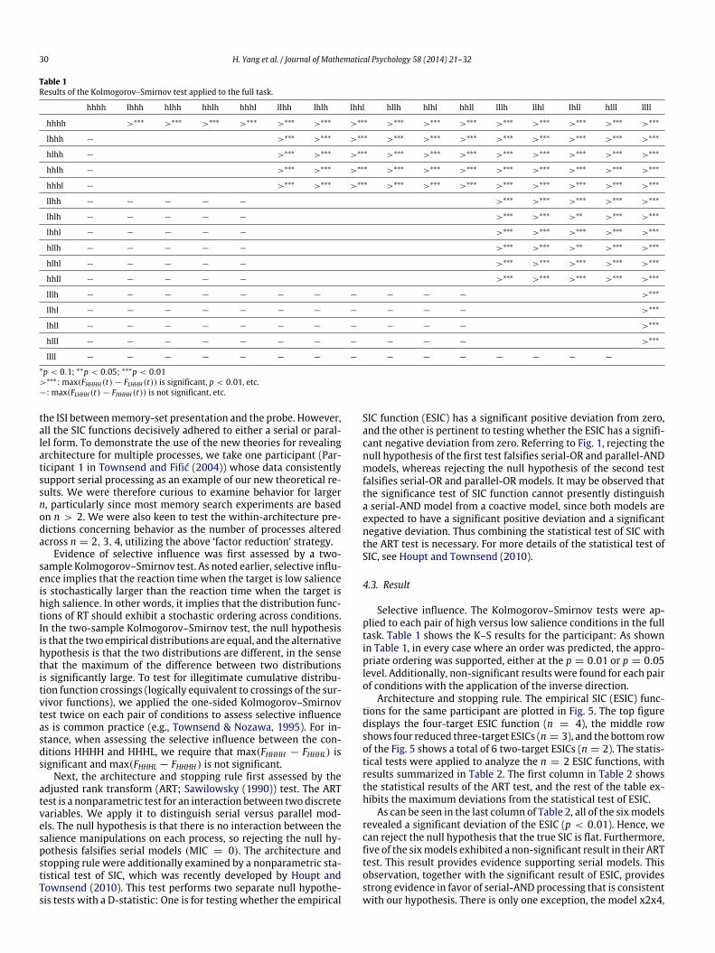
Evidence of selective influence was first assessed by a two-sample Kolmogorov–Smirnov test. As noted earlier, selective influ-ence implies that the reaction time when the target is low salienceis stochastically larger than the reaction time when the target ishigh salience. In other words, it implies that the distribution func-tions of RT should exhibit a stochastic ordering across conditions.In the two-sample Kolmogorov–Smirnov test, the null hypothesisis that the twoempirical distributions are equal, and the alternativehypothesis is that the two distributions are different, in the sensethat the maximum of the difference between two distributionsis significantly large. To test for illegitimate cumulative distribu-tion function crossings (logically equivalent to crossings of the sur-vivor functions), we applied the one-sided Kolmogorov–Smirnovtest twice on each pair of conditions to assess selective influenceas is common practice (e.g., Townsend & Nozawa, 1995). For in-stance, when assessing the selective influence between the con-ditions HHHH and HHHL, we require that max(FHHHH − FHHHL) issignificant and max(FHHHL − FHHHH) is not significant.

Next, the architecture and stopping rule first assessed by theadjusted rank transform (ART; Sawilowsky (1990)) test. The ARTtest is a nonparametric test for an interaction between twodiscretevariables. We apply it to distinguish serial versus parallel mod-els. The null hypothesis is that there is no interaction between thesalience manipulations on each process, so rejecting the null hy-pothesis falsifies serial models (MIC = 0). The architecture andstopping rule were additionally examined by a nonparametric sta-tistical test of SIC, which was recently developed by Houpt andTownsend (2010). This test performs two separate null hypothe-sis tests with a D-statistic: One is for testing whether the empirical

SIC function (ESIC) has a significant positive deviation from zero,and the other is pertinent to testing whether the ESIC has a signifi-cant negative deviation from zero. Referring to Fig. 1, rejecting thenull hypothesis of the first test falsifies serial-OR and parallel-ANDmodels, whereas rejecting the null hypothesis of the second testfalsifies serial-OR and parallel-OR models. It may be observed thatthe significance test of SIC function cannot presently distinguisha serial-AND model from a coactive model, since both models areexpected to have a significant positive deviation and a significantnegative deviation. Thus combining the statistical test of SIC withthe ART test is necessary. For more details of the statistical test ofSIC, see Houpt and Townsend (2010).

4.3. Result

Selective influence. The Kolmogorov–Smirnov tests were ap-plied to each pair of high versus low salience conditions in the fulltask. Table 1 shows the K–S results for the participant: As shownin Table 1, in every case where an order was predicted, the appro-priate ordering was supported, either at the p = 0.01 or p = 0.05level. Additionally, non-significant results were found for each pairof conditions with the application of the inverse direction.

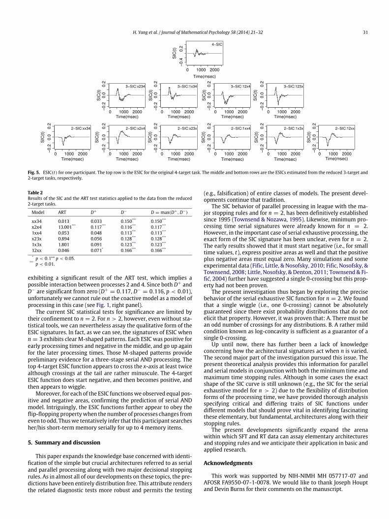
Architecture and stopping rule. The empirical SIC (ESIC) func-tions for the same participant are plotted in Fig. 5. The top figuredisplays the four-target ESIC function (n = 4), the middle rowshows four reduced three-target ESICs (n = 3), and the bottom rowof the Fig. 5 shows a total of 6 two-target ESICs (n = 2). The statis-tical tests were applied to analyze the n = 2 ESIC functions, withresults summarized in Table 2. The first column in Table 2 showsthe statistical results of the ART test, and the rest of the table ex-hibits the maximum deviations from the statistical test of ESIC.

As can be seen in the last column of Table 2, all of the sixmodelsrevealed a significant deviation of the ESIC (p < 0.01). Hence, wecan reject the null hypothesis that the true SIC is flat. Furthermore,five of the sixmodels exhibited a non-significant result in their ARTtest. This result provides evidence supporting serial models. Thisobservation, together with the significant result of ESIC, providesstrong evidence in favor of serial-AND processing that is consistentwith our hypothesis. There is only one exception, the model x2x4,


Fig. 5. ESIC(t) for one participant. The top row is the ESIC for the original 4-target task. The middle and bottom rows are the ESICs estimated from the reduced 3-target and2-target tasks, respectively.

Table 2Results of the SIC and the ART test statistics applied to the data from the reduced2-target tasks.

Model ART D+ D− D = max(D+,D−)

xx34 0.013 0.033 0.150*** 0.150***

x2x4 13.001*** 0.117*** 0.116*** 0.117***

1xx4 0.053 0.048 0.113*** 0.113***

x23x 0.894 0.056 0.128*** 0.128***

1x3x 1.801 0.091 0.123*** 0.123***

12xx 0.046 0.071* 0.166*** 0.166***

* p < 0.1** p < 0.05.*** p < 0.01.

exhibiting a significant result of the ART test, which implies apossible interaction between processes 2 and 4. Since both D+ andD− are significant from zero (D+

= 0.117, D−= 0.116, p < 0.01),

unfortunately we cannot rule out the coactive model as a model ofprocessing in this case (see Fig. 1, right panel).

The current SIC statistical tests for significance are limited bytheir confinement to n = 2. For n > 2, however, even without sta-tistical tools, we can nevertheless assay the qualitative form of theESIC signatures. In fact, as we can see, the signatures of ESIC whenn = 3 exhibits clear M-shaped patterns. Each ESIC was positive forearly processing times and negative in the middle, and go up againfor the later processing times. Those M-shaped patterns providepreliminary evidence for a three-stage serial AND processing. Thetop 4-target ESIC function appears to cross the x-axis at least twicealthough crossings at the tail are rather minuscule. The 4-targetESIC function does start negative, and then becomes positive, andthen appears to wiggle.

Moreover, for each of the ESIC functionswe observed equal pos-itive and negative areas, confirming the prediction of serial ANDmodel. Intriguingly, the ESIC functions further appear to obey theflip-flopping propertywhen the number of processes changes fromeven to odd. Thuswe tentatively infer that this participant searchesher/his short-term memory serially for up to 4 memory items.

5. Summary and discussion

This paper expands the knowledge base concerned with identi-fication of the simple but crucial architectures referred to as serialand parallel processing along with two major decisional stoppingrules. As in almost all of our developments on these topics, the pre-dictions have been entirely distribution free. This attribute rendersthe related diagnostic tests more robust and permits the testing

(e.g., falsification) of entire classes of models. The present devel-opments continue that tradition.

The SIC behavior of parallel processing in league with the ma-jor stopping rules and for n = 2, has been definitively establishedsince 1995 (Townsend & Nozawa, 1995). Likewise, minimum pro-cessing time serial signatures were already known for n = 2.However, in the important case of serial exhaustive processing, theexact form of the SIC signature has been unclear, even for n = 2.The early results showed that it must start negative (i.e., for smalltime values, t), express positive areas as well and that the positiveplus negative areas must equal zero. Many simulations and someexperimental data (Fific, Little, & Nosofsky, 2010; Fific, Nosofsky, &Townsend, 2008; Little, Nosofsky, & Denton, 2011; Townsend & Fi-fić, 2004) further have suggested a single 0-crossing but this prop-erty had not been proven.

The present investigation thus began by exploring the precisebehavior of the serial exhaustive SIC function for n = 2. We foundthat a single wiggle (i.e., one 0-crossing) cannot be absolutelyguaranteed since there exist probability distributions that do notelicit that property. However, it was proven that: A. There must bean odd number of crossings for any distributions. B. A rather mildcondition known as log-concavity is sufficient as a guarantor of asingle 0-crossing.

Up until now, there has further been a lack of knowledgeconcerning how the architectural signatures act when n is varied.The second major part of the investigation pursued this issue. Thepresent theoretical analysis provides this information for paralleland serial models in conjunction with both theminimum time andmaximum time stopping rules. Although in some cases the exactshape of the SIC curve is still unknown (e.g., the SIC for the serialexhaustive model for n > 2) due to the flexibility of distributionforms of the processing time, we have provided thorough analysisspecifying critical and differing traits of SIC functions underdifferent models that should prove vital in identifying fascinatingthese elementary, but fundamental, architectures along with theirstopping rules.

The present developments significantly expand the arenawithin which SFT and RT data can assay elementary architecturesand stopping rules and we anticipate their application in basic andapplied research.

Acknowledgments

This work was supported by NIH-NIMH MH 057717-07 andAFOSR FA9550-07-1-0078. We would like to thank Joseph Houptand Devin Burns for their comments on the manuscript.


References

Atkinson, R., Holmgren, J., & Juola, J. (1969). Processing time as influenced by thenumber of elements in a visual display. Attention, Perception, & Psychophysics,6, 321–326.

Atkinson, R. C., & Estes, W. K. (1963). Stimulus sampling theory. In R. D. Luce,R. R. Bush, & E. Galanter (Eds.), Handbook of mathematical psychology (vol. 2).New York: Wiley.

Broadbent, D. E. (1958). Perception and communication. New York: OxfordUniversity Press.

Cherry, E. C. (1953). Some experiments on the recognition of speech, with one andwith two ears. Journal of the Acoustical Society of America, 25, 975–979.

Chung, K. L. (1953). Sur les lois de probabilites unimodales. Comptes Rendus del’Academie des Sciences, 236, 583–584.

Dharmadhikari, S. W., & Joag-Dev, K. (1988). Unimodality, convexity, and applica-tions. Academic Press.

Donders, F. C. (1868). Over de snelheid van psychische processen. Onderzoekingengedaan in het physiologisch laboratorium der Utrechtsche hoogeschool,1868–1869. Tweeds Reeks, II , 92–120.

Dzhafarov, E. N. (1997). Process representations and decompositions of responsetimes. In A. A. J. Marley (Ed.), Choice, decision and measurement: essays in honorof R. Duncan Luce. Mahwah, NJ: Erlbaum.

Dzhafarov, E. N. (1999). Conditionally selective dependence of random variables onexternal factors. Journal of Mathematical Psychology, 43, 123–157.

Dzhafarov, E. N. (2003). Selective influence through conditional independence.Psychometrica, 68, 7–25.

Dzhafarov, E. N., Schweickert, R., & Sung, K. (2004). Mental architectures withselectively influenced but stochastically interdependent components. Journalof Mathematical Psychology, 48, 51–64.

Egeth, H. E. (1966). Parallel versus serial processes in multidimensional stimulusdiscrimination. Attention, Perception, & Psychophysics, 1, 245–252.

Eriksen, C. W., & Spencer, T. R. (1969). Rate of information processing invisual perception: some results and methodological considerations. Journal ofExperimental Psychology Monographs, 79, 1–16.

Estes, W. K. (1955). Statistical theory of spontaneous recovery and regression.Psychological Review, 62(3), 145–154.

Estes, W. K. (1959). The statistical approach to learning theory. In S. Koch (Ed.),Psychology: a study of a science (vol. 2). New York: McGraw-Hill.

Estes, W. K., & Taylor, H. A. (1964). A detectionmethod and probabilistic models forassessing information processing from brief visual displays. Proceedings of theNational Academy of Science, 52, 446–454.

Estes, W. K., & Taylor, H. A. (1966). Visual detection in relation to display size andredundancy of critical elements. Perception and Psychophysics, 1, 9–16.

Estes, W. K., & Wessel, D. L. (1966). Reaction time in relation to display size andcorrectness of response in forced-choice visual signal detection. Perception andPsychophysics, 1, 369–373.

Fific, M., Little, D. R., & Nosofsky, R. M. (2010). Logical-rule models of classificationresponse times: a synthesis of mental-architecture, random-walk, anddecision-bound approaches. Psychological Review, 117, 309–348.

Fific, M., Nosofsky, R. M., & Townsend, J. T. (2008). Information-processingarchitectures in multidimensional classification: a validation test of thesystems factorial technology. Journal of Experimental Psychology: HumanPerception and Performance, 34, 356–375.

Friedman, M. P., Burke, C. J., Cole, M., Keller, L., Millward, R. B., & Estes, W. K. (1964).Two-choice behavior under extended training with shifting probabilities ofreinforcement. In R. C. Atkinson (Ed.), Studies in mathematical psychology.Stanford, CA: Stanford University Press.

Garner, W. R. (1962). Uncertainty and structure as psychological concepts. New York:Wiley.

Green, D. M., & Swets, J. A. (1966). Signal detection theory and psychophysics.Huntington, N.Y.: Krieger.

Haber, R. N., & Hershenson, M. (1973). The psychology of visual perception. Oxford,England: Holt, Rinehart & Winston.

Hick, W. E. (1952). On the rate of gain of information. Quarterly Journal ofExperimental Psychology, 4, 11–36.

Houpt, J. W., & Townsend, J. T. (2010). The statistical properties of the survivorinteraction contrast. Journal of Mathematical Psychology, 54, 446–453.

Hull, C. L. (1952). A behavior system: an introduction to behavior theory concerningthe individual organism. New Haven, CT, US: Yale University Press.

Ibragimov, I. A. (1956). On the composition of unimodal distributions. Theory ofProbability and its Applications, 1, 255–360.

Koch, S. (1954). Clark l. Hull. In W. K. Estes, S. Koch, K. MacCorquodale, P. E. Meehl,C. G.Mueller,W. N. Schoenfeld, &W. S. Verplanck (Eds.),Modern learning theory.East Norwalk, CT, US: Appleton-Century-Crofts.

Krantz, D. H., Luce, R. D., Suppes, P., & Tversky, A. (1971). Foundations ofmeasurement (vol. 1.). New York: Academic Press.

Kujala, J. V., & Dzhafarov, E. N. (2008). Testing for selectivity in the dependence ofrandom variables on external factors. Journal of Mathematical Psychology, 52,128–144.

Little, D. R., Nosofsky, R. M., & Denton, S. E. (2011). Response-time tests of logical-rule models of categorization. Journal of Experimental Psychology: Learning,Memory, and Cognition, 37, 1–27.

Murdock, B. B. (1971). A parallel-processing model for scanning. Attention,Perception, & Psychophysics, 10, 289–291.

Nickerson, R. S. (1972). Binary-classification reaction time: a review of somestudies of human information-processing capabilities. Psychonomic MonographSupplements, 4, 275–318.

Posner, M. I. (1978). Chronometric explorations of mind. NJ: Erlbaum: EnglewoodHeights.

Roberts, P., & Zinnes, J. L. (1963). In R. R. B. R. D. Luce, & E. Galanter (Eds.), Handbookof mathematical psychology (vol. 1). New York: Wiley.

Sawilowsky, S. S. (1990). Nonparametric tests of interaction in experimental design.Review of Educational Research, 60, 91–126.

Scharff, A., Palmer, J., &Moore, C.M. (2011). Extending the simultaneous-sequentialparadigm to measure perceptual capacity for features and words. Journal ofExperimental Psychology: Human Perception and Performance, 37, 813–833.

Schweickert, R. (1978). A critical path generalization of the additive factor method:analysis of a Stroop task. Journal of Mathematical Psychology, 18, 105–139.

Schweickert, R. (1982). The bias of an estimate of coupled slack in stochastic pertnetworks. Journal of Mathematical Psychology, 26, 1–12.

Schweickert, R., & Giorgini, M. (1999). Response time distributions: some simpleeffects of factors selectively influencingmental processes. Psychonomic Bulletin& Review, 6, 269–288.

Schweickert, R., Giorgini, M., & Dzhafarov, E. N. (2000). Selective influenceand response time cumulative distribution functions in serial-parallel tasknetworks. Journal of Mathematical Psychology, 44, 504–535.

Schweickert, R., & Townsend, J. T. (1989). A trichotomy interactions of factorsprolonging sequential and concurrent mental processes in stochastic discretemental (pert) networks. Journal of Mathematical Psychology, 33, 328–347.

Schweickert, R., & Wang, Z. (1993). Effects on response time of factors selectivelyinfluencing processing in acyclic task networks with or gates. British Journal ofMathematical and Statistical Psychology, 46, 1–30.

Sperling, G. (1960). The information available in brief visual presentations.Psychological Monographs General and Applied, 74, 1–29.

Sperling, G. (1967). Successive approximations to a model for short-termmemory.In A. Sanders (Ed.), Attention and performance. Amsterdam: North- Holland.

Sternberg, S. (1966). High-speed scanning in human memory. Science, 153, 652.Sternberg, S. (1969). The discovery of processing stages: extensions of Donders’

method. Acta Psychologica, 30, 276–315.Sternberg, S. (1975). Memory scanning: new findings and current controversies.

Quarterly Journal of Experimental Psychology, 27, 1–32.Tanner, W. P., & Swets, J. A. (1954). A decision-making theory of visual detection.

Psychological Review, 61, 401–409.Townsend, J.T. (1969). Stochastic representations of serial and parallel processes.

In Paper presented at Midwest Mathematical Psychology Meetings, IndianaUniversity.

Townsend, J. T. (1971). A note on the identifiability of parallel and serial processes.Attention, Perception, & Psychophysics, 10, 161–163.

Townsend, J. T. (1972). Some results concerning the identifiability of parallel andserial processes. British Journal of Mathematical and Statistical Psychology, 25,168–199.

Townsend, J. T. (1974). Issues and models concerning the processing of a finitenumber of inputs. In B. Kantowitz (Ed.), Human information processing .Hillsdale, NJ: Erlbaum Press.

Townsend, J. T. (1976). Serial and within-stage independent parallel modelequivalence on the minimum completion time. Journal of MathematicalPsychology, 14, 219–238.

Townsend, J. T. (1981). Some characteristics of visual whole report behavior. ActaPsychologica, 47, 149–173.

Townsend, J. T. (1984). Uncovering mental processes with factorial experiments.Journal of Mathematical Psychology, 28, 363–400.

Townsend, J. T. (1990a). Serial vs. parallel processing: sometimes they look likeTweedledum and Tweedledee but they can (and should) be distinguished.Psychological Science, 1, 46–54.

Townsend, J. T. (1990b). Truth and consequences of ordinal differences in statisticaldistributions: toward a theory of hierarchical inference. Psychological Bulletin,108, 551–567.

Townsend, J. T. (1992). Don’t be fazed by phaser: beginning exploration of a cyclicalmotivational system. Behavior Research Methods, Instruments, & Computers, 24,219–227.

Townsend, J. T., & Ashby, F. G. (1983). The stochastic modeling of elementarypsychological processes. Cambridge: Cambridge University Press.

Townsend, J. T., & Fifić, M. (2004). Parallel versus serial processing and individualdifferences in high-speed search in human memory. Attention, Perception, &Psychophysics, 66, 953–962.

Townsend, J. T., Fific, M., & Neufeld, R. W. J. (2007). Assessment of mental archi-tecture in clinical/cognitive research. In T. A. Treat, R. R. Bootzin, & T. B. Baker(Eds.), Psychological clinical science: papers in honor of Richard M. Mcfall. Mah-wah, NJ: Lawrence Erlbaum Associates.

Townsend, J. T., & Nozawa, G. (1995). Spatio-temporal properties of elementaryperception: an investigation of parallel, serial, and coactive theories. Journal ofMathematical Psychology, 39, 321–359.

Townsend, J. T., & Thomas, R. (1994). Stochastic dependencies in parallel andserial models: effects on systems factorial interactions. Journal of MathematicalPsychology, 38, 1–34.

Townsend, J. T., & Wenger, M. J. (2004). A theory of interactive parallel processing:new capacity measures and predictions for a response time inequality series.Psychological Review, 111, 1003–1035.

Townsend, J. T., Yang, H., & Burns, D. M. (2011). Experimental discrimination ofthe world’s simplest and most antipodal models: the parallel-serial issue. InH. Colonius, & E. N. Dzhafarov (Eds.), Descriptive and normative approaches tohuman behavior in the advanced series on mathematical psychology. Singapore:World Scientific.

Vorberg, D. (1977). On the equivalence of parallel and serial models of informationprocessing. In Paper presented at the tenth annual mathematical psychologicalmeeting.

http://refhub.elsevier.com/S0022-2496(13)00122-3/sbref1


































































survivor interaction contrast wiggle predictions of

Documents