Suspense and Surprise∗

Jeffrey ElyNorthwestern University

Alexander FrankelUniversity of Chicago

Emir KamenicaUniversity of Chicago

October 2012

Abstract

We model demand for non-instrumental information, drawing on the idea that peoplederive entertainment utility from suspense and surprise. A period has more suspenseif the variance of the next period’s beliefs is greater. A period has more surprise ifthe current belief is further from the last period’s belief. Under these definitions, weanalyze the optimal way to reveal information over time so as to maximize expectedsuspense or surprise experienced by a Bayesian audience. We apply our results to thedesign of mystery novels, political primaries, casinos, game shows, auctions, and sports.

∗We would like to thank J.P. Benoit, Eric Budish, Sylvain Chassang, Eddie Dekel, Matthew Gentzkow,Ben Golub, Navin Kartik, Scott Kominers, Michael Ostrovsky, Devin Pope, Jesse Shapiro, Joel Sobel, andSatoru Takahashi for helpful comments. Jennifer Kwok, Ahmad Peivandi, and David Toniatti providedexcellent research assistance. We thank the William Ladany Faculty Research Fund and the Initiative onGlobal Markets at the University of Chicago Booth School of Business for financial support.

1

presented by Emir KamenicaFRIDAY, Mar. 8, 20131:30 pm - 3:00 pm, Room: HOH-706

USC FBE APPLIED ECONOMICS WORKSHOP

1 Introduction

People frequently seek non-instrumental information. They follow international news and

sports even when no contingent actions await. We postulate that a component of this

demand for non-instrumental information is its entertainment value. It is exciting to refresh

the New York Times webpage to find out whether Gaddafi has been captured and to watch

a baseball pitch with full count and bases loaded.

In this paper, we formalize the idea that information provides entertainment and we

analyze the optimal way to reveal information over time so as to maximize expected sus-

pense or surprise experienced by a rational Bayesian audience. Our analysis informs two

distinct sets of issues.

First, in a number of industries, provision of entertainment is a crucial service. Mystery

novels, soap operas, sports events, and casinos all create value by revealing information over

time in a manner that makes the experience more exciting. Of course, in each of these cases

information revelation is bundled with other valuable features of the good – elegant prose,

skilled acting, impressive athleticism, attractive waitstaff – but information revelation is

the common component of these seemingly disparate industries. Moreover, entertainment

is an important part of modern life. The American Time Use Survey reveals that adults in

the United States spend roughly one fifth of their waking hours consuming entertainment

(Aguiar, Hurst, and Karabarbounis (2011)).

Second, even if obtained for non-instrumental reasons, information can have substan-

tial social consequences. Consider politics. As Downs (1957) has emphasized, the efficacy

of democratic political systems is limited by voters’ ignorance. This is particularly prob-

lematic because individual voters, who are unlikely to be pivotal, have little instrumental

reason to obtain information about the candidates. Despite this lack of a direct incentive,

many voters do in fact follow political news and watch political debates, thus becoming an

informed electorate. A potential explanation is that the political process unfolds in a way

that generates enjoyable suspense and surprise. Developing models of entertainment-based

demand for non-instrumental information will thus inform the analysis of social issues, such

as voting, that seem unrelated to entertainment.

In our model, there is a finite state space and a finite number of periods. The principal

(the designer) reveals information about the state to the agent (the audience) over time.

Specifically, the principal chooses the information policy: signals about the state, contin-

gent on the current period and the current belief. The agent observes the realization of each

2

signal and forms beliefs by Bayes’ rule. The agent has preferences over the stochastic path

of his beliefs. A period generates more suspense if the variance of next period’s beliefs is

greater. A period generates more surprise if the current belief is further from last period’s

belief. The agent’s utility in each period is an increasing function of suspense or surprise

experienced in that period, and the principal seeks to maximize the expected undiscounted

sum of per-period utilities.

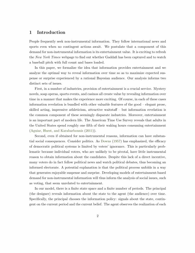
To fix ideas, consider Figure 1 below. We plot the path of estimated beliefs about the

winners of the 2011 US Open Semifinals over the course of these two tennis matches. Panel

(a) shows Djokovic versus Federer, and Panel (b) shows Murray versus Nadal.1 The match

between Djokovic and Federer was exciting, with dramatic lead changes and key missed

opportunities; Federer had multiple match points but went on to lose. In contrast, there

was much less drama between Murray and Nadal, as Nadal dominated from the outset.

Our model formalizes the notion that Federer-Djokovic generated more suspense and more

surprise than Murray-Nadal.

Figure 1: 2011 US Open Semifinals

0 50 100 150 200 250 300

0.0

0.5

1.0

Point

Pro

babi

lity

of W

in

(a) Likelihood that Djokovic beats Federer

0 50 100 150 200

0.0

0.5

1.0

Point

Pro

babi

lity

of W

in

(b) Likelihood that Murray beats Nadal

We consider the problem of designing an optimal information policy, subject to a given

prior and number of periods. We show that the suspense-optimal policy leads to decreasing

residual uncertainty over time. Suspense is constant across periods and there is no variabil-

ity in ex post suspense. This constant suspense is generated by asymmetric belief-swings

– “plot twists” – which become both larger and less likely as time passes. The state is not

fully revealed until the final period. One implication of our results is that most existing

1We estimate the likelihood of victory given the current score using a simple model which assumes thatthe serving player wins the point with probability 0.64 (the overall fraction of points won by serving playersin the tournament). The data and methodology are drawn from jeffsackmann.com.

3

sports cannot be suspense-optimal; we offer specific guidance on rules that would make

sports more suspenseful.

Assuming additional structure, we also study the information policy that maximizes

expected surprise. Under this policy, residual uncertainty may go up or down over time.

Surprise in each period is variable, as is the ex post total surprise. In contrast to the

suspense-optimal policy, when there are many periods the beliefs shift only a small amount

in each period. There is a positive probability that the state is fully revealed before the

final period. These features imply that a surprise-optimizing principal faces substantial

commitment problems.

The previous results apply to the setting where the principal has no constraints on

the technology by which she reveals information to the agent. We also briefly consider

some specific constrained problems such as seeding teams in a tournament, determining

the number of games in a finals series, and ordering sequential contests such as political

primaries.

Our paper connects with four lines of research. It primarily contributes to the nascent

literature on the design of informational environments. Kamenica and Gentzkow (2011)

consider a static version of our model2 where a principal chooses an arbitrary signal to

reveal to an agent, who then takes an action that affects the welfare of both players. In

that case, the principal has a value function over the agent’s single-period posterior;3 our

principal has a value function over the agent’s multi-period belief martingale. In this

sense our model shares features with Horner and Skrzypacz (2011) who study a privately

informed agent who is selling information to an investor. A scheme in which the agent sells

information gradually maximizes the agent’s ex ante incentives to acquire information.

In a broader sense, our paper also contributes to the literature on micro-foundations of

preferences. Stigler and Becker (1977) advocate a research agenda of decomposing seem-

ingly fundamental preferences into their constituent parts. This approach has been applied

in a variety of settings, e.g., to demand for advertised (Becker and Murphy (1993)) and

addictive (Becker and Murphy (1988)) goods. We apply it to drama-based entertainment.

At first glance it may seem that the question of why one mystery novel is more enjoy-

able than another or the question of what makes a sports game exciting is outside the

2Brocas and Carrillo (2007), Rayo and Segal (2009), and Tamura (2012) examine special cases of thisstatic model.

3A separate literature posits that agents have a direct preference for particular beliefs (e.g.,Akerlof andDickens (1982)); a number of papers analyze whether such preferences lead to demand for non-instrumentalinformation (e.g., Eliaz and Spiegler (2006), Eliaz and Schotter (2010)).

4

purview of economics; such judgments may seem based on tastes that are inscrutable, like

the preference for vanilla over chocolate ice cream. As our analysis reveals, however, recon-

ceptualizing these judgments as being (partly) based on a taste for suspense and surprise

reveals new insights about entertainment and demand for non-instrumental information

more generally.

Third, our paper contributes to the literature on preferences over the timing of resolu-

tion of uncertainty. The original treatment of this subject goes back to Kreps and Porteus

(1978). They axiomatize a representation of preferences for early or late resolution. Caplin

and Leahy (2001) apply this framework to a setting where individuals have preferences

over anticipatory emotions. They point out that agents might bet on their favorite team so

as to increase the amount of suspense they will experience while watching a sports game.

Koszegi and Rabin (2009) and Dillenberger (2010) model agents who prefer one-shot rather

than gradual revelation of information.

Finally, there is a small formal literature on suspense and surprise per se. Chan, Courty,

and Li (2009) define suspense as valuing contestants’ efforts more when the game is close

and demonstrate that preference for suspense increases the appeal of rank-order incentive

schemes over linear ones. The definition of surprise of Geanakoplos (1996) is similar to

ours. He considers a psychological game (Geanakoplos, Pearce, and Stacchetti (1989))

where a principal wants to surprise an agent. Specifically, he examines the Hangman’s

Paradox (Gardner (1969)), the problem of choosing a date on which to hang a prisoner so

that the prisoner is surprised. In his setting, the principal has no commitment power, so

surprise is not possible in equilibrium. Borwein, Borwein, and Marechal (2000) give the

principal commitment power, and derive the surprise-optimal probabilities for hanging at

each date.4

The remainder of the paper is structured as follows. Section 2 presents the model.

Section 3 discusses the interpretation of the model. Section 4 and Section 5 derive the

suspense- and surprise-optimal information policies. Section 6 compares these policies.

Section 7 considers constrained problems. Section 8 concludes.

4Let pt denote the conditional probability of being hanged on day t, given that the prisoner is still alive.They define surprise in period t as the entropy (− log pt) if the prisoner is hanged, and 0 otherwise.

5

2 A model of suspense and surprise

We develop a model in which a principal reveals information over time about the state of

the world to an agent.

2.1 Preferences, beliefs, and technology

There is a finite state space Ω. A typical state is denoted ω. A typical belief is denoted by

µ ∈ ∆ (Ω); µω designates the probability of ω. The prior is µ0. Let t ∈ 0, 1, ..., T denote

the period.

A signal π maps the state to a distribution over a finite signal realization space S, i.e.,

π : Ω → ∆ (S). An information policy π is a function that maps the current period and

the current belief into a signal. Let Π denote the set of all information policies.5

Any information policy generates a stochastic path of beliefs about the state. A belief

martingale µ is a sequence (µt)Tt=0 s.t. (i) µt ∈ ∆ (∆ (Ω)) for all t, (ii) µ0 is degenerate

at µ0, and (iii) E [µt | µ0, ..., µt−1] = µt−1 for all t ∈ 1, ..., T. A realization of a belief

martingale is a belief path η = (µt)Tt=0. Given the current belief µt, a signal induces a

distribution of posteriors µt+1 s.t. E [µt+1] = µt. Hence, an information policy induces a

belief martingale. We denote the belief martingale induced by information policy π (given

the prior µ0) by 〈π | µ0〉.There are two players: the agent and the principal. The agent has preferences over his

belief path and the belief martingale. The agent has a preference for suspense if his utility

function is

Ususp (η, µ) =

T−1∑t=0

u

(Et∑ω

(µωt+1 − µωt

)2)for some increasing function u (·) with u(0) = 0. An agent has a preference for surprise if

her utility function is

Usurp (η) =

T∑t=1

u

(∑ω

(µωt − µωt−1

)2)for some increasing function u (·) with u(0) = 0. So suspense is induced by variance over

the next period’s beliefs, and surprise by change from the previous belief to the current

5The assumption that S is finite is innocuous since Ω is finite. The assumption that π depends only onthe current belief and period, rather than the full history, is without loss of generality in the sense thatmemoryless policies do not restrict the set of feasible outcomes.

6

one.

We will frequently focus on the baseline specification where suspense is the standard

deviation of µt+1 (aggregated across states) and surprise is the Euclidean distance between

µt and µt−1. This corresponds to setting u(x) =√x.

The principal chooses the information policy to maximize the agent’s expected utility.

If the agent has a preference for suspense, the principal solves

maxπ∈Π

E〈π|µ0〉Ususp (η, 〈π | µ0〉) .

If the agent has a preference for surprise, the principal solves

maxπ∈Π

E〈π|µ0〉Usurp (η) .

Note that the choice of the information policy affects the value of the objective function

only through the belief martingale it induces. The additional details of the information

policy are irrelevant for payoffs. Thus, it is convenient to recast the optimization problem

as a direct choice of the belief martingale. An extension of the argument in Proposition

1 of Kamenica and Gentzkow (2011) shows that any belief martingale can be induced by

some information policy.6

Lemma 1. Given any belief martingale µ, there exists an information policy π such that

µ = 〈π | µ0〉 .

In some settings the set of feasible information policies might be limited by tradition,

complexity, or other institutional constraints. For example, the organizer of a tournament

may have settled on an elimination format and is choosing between seeding procedures. Or

a political party respects the rights of states to choose their own delegates, but may have

control over the order in which states hold elections. Accordingly, let P ⊂ Π × (∆Ω) × Nbe a subset of the Cartesian product of information policies, priors, and durations. In

Section 7 we consider a constrained model in which the principal chooses (π, µ0, T ) ∈ P so

as to maximize expected suspense or surprise.

6Kamenica and Gentzkow show in a static model that, when current belief is µt, any distribution ofposteriors µt+1 with mean µt can be induced by some signal. Applying this result period-by-period yieldsour Lemma 1.

7

2.2 Extensions

There are some natural extensions to our specification of the agent’s utility function.

First and most obvious, the audience might value both suspense and surprise. While

we cannot fully characterize the optimal information policy for such preferences, we discuss

the tradeoff between suspense and surprise in Section 6.

Second, the audience would presumably have a distinct preference for learning the

outcome by the end, i.e., from having µT degenerate. Including this term in the utility

function would not have any effect on our results since any suspense- or surprise-maximizing

policy reveals the state by the last period.

Third, the audience may experience additional utility from the realization of a particular

state. For example, a sports fan enjoys games that are exciting, but is particularly happy

should her team win. We can incorporate this in our model by supposing that the overall

utility is a sum of the utility from suspense/surprise and a utility from the final belief being

degenerate at some state. Such a modification does not affect the optimal policy; it only

changes the payoff-maximizing prior.

Fourth, one may consider models with state-dependent significance where the audience

cares more about changes in the likelihood of particular states. For instance, the reader

of a mystery novel may be in great suspense about whether the protagonist committed

the murder. But in the event of the protagonist’s innocence, she cares less about whether

the murderer was Stooge A or Stooge B. Or, if the New York Yankees have five times

the audience of the Milwaukee Brewers, the league may value suspense/surprise about the

Yankees’ championship prospects five times as much as suspense about the Brewers. We

can accordingly modify suspense utility to be

Ususp (η, µ) =T−1∑t=0

u

(Et∑ω

αω ·(µωt+1 − µωt

)2),

and likewise for surprise. More important characters or larger market sports teams have a

larger state-dependent weight αω ≥ 0.

Fifth, the audience might weigh suspense and surprise differently across periods. For

example, later periods might be weighted more heavily if the reader becomes more in-

vested in the characters as she advances through the novel. In models with time-dependent

8

significance, we replace suspense utility with

Ususp (η, µ) =T−1∑t=0

βtu

(Et∑ω

(µωt+1 − µωt

)2),

and again likewise for surprise. A period in which the audience is more involved has a

higher value of βt ≥ 0. In Section 4, we discuss the suspense-optimal information policies

in cases of state- or time-dependent significance.

Finally, sometimes the agent might be invested only in some aspect of her belief such as

the expectation. Consider a gambler who plays a sequence of fair gambles and experiences

suspense (or surprise) when her expected earnings from the visit are about to change

(or just did). Formally, ω is a bounded random variable and the agent has preferences

over the path of its expectation; e.g., in case of surprise, agent’s utility in period t is

u(Eµt [ω]− Eµt−1 [ω]

)2. While we will not discuss this extension at length, all of our

results apply in this case as well.

3 The interpretation of the model

Before we proceed with the derivation of optimal information policies, we discuss some of

the potential interpretations of the model above.

3.1 Interpretation of the technology

Suppose that the principal is a publishing house and the agent is a reader of mystery

novels. In this case, a writer is associated with a belief martingale, and a particular book

by writer µ is a belief path η drawn from µ. For a concrete example, say that Mrs. X is

a writer and all of her books follow a similar premise. In the opening pages of the novel,

a dead body is found at a remote country house where n guests and staff are present. In

every novel by Mrs. X, one of these n individuals single-handedly committed the murder.7

The opening pages establish a prior µ0 over the likelihood that each individual ω ∈ Ω is

the culprit. There are then T chapters each revealing some information about the identity

7In Mrs. X’s novels, it is never the case that the murderer is someone the reader has not been introducedto at the outset. This allows us to model uncertainty in a classical way without addressing issues ofunawareness. We could easily allow, however, for the possibility that the murder was really a suicide(change n to n + 1) or, as in Murder on the Orient Express, that (spoiler alert) several of the suspectsjointly committed the murder (change n to 2n − 1).

9

of the murderer. A literal (though perhaps not very literary) interpretation is that Mrs.

X explicitly randomizes the plot of each chapter based on her information policy and her

current belief (based on the content she has written thus far) and learns whodunnit only

when she completes the novel.8

Alternatively, the principal is the rule-setting body of a sports association and the agent

is a sports fan. In this case, we associate the feasible set of rules with some constraint set

P , the chosen rule with an information policy π, a match-up with a prior and a belief

martingale 〈π | µ0〉, and a match with a belief path η. To see how modifying the rules

changes the information policy, note that if it becomes more difficult to score as players

get tired, rules that permit fewer substitutions increase the amount of information that is

revealed in the earlier periods. Or, if it is easier to score when fewer players are on the field,

rules that lower the threshold for issuing red cards may reveal more information later in

the game. The rules of a sport also affect priors and belief martingales through the players’

strategic responses to such rules. For instance, actions with low expected value but high

variance may be played at the end of the game but will never be played at the beginning,

e.g., 2-point conversions in football. Allowing such actions can alter the relative amount

of information revealed early versus late. Different rules might also induce different priors.

For instance, a worse tennis player will have a higher chance of winning under the tie-break

rule for deciding sets.

Our model captures settings both where the state is realized ex ante and those where

it is realized ex post. An example where ω is realized ex ante is a game show where

a contestant receives either an empty or a prize-filled suitcase, and then information is

slowly revealed about the suitcase’s contents. In presidential primaries, on the other hand,

ω is realized ex post. Whichever candidate gets more than 50% of the overall delegates wins

the nomination. When a candidate wins a state’s delegates, this outcome provides some

information about whether she will win the nomination. In this case the state ω is not an

aspect of the world that is fixed at the outset; it is determined by the signal realizations

themselves.

Implicit in our formal structure is the assumption that the principal and the agent share

8This interpretation brings to mind the notion of “willful characters.” For example, novelist Jodi Picoultwrites, “Often, about 2/3 of the way through, the characters will take over and move the book in a differentdirection. I can fight them, but usually when I do that the book isn’t as good as it could be. It soundscrazy, but the book really starts writing itself after a while. I often feel like I’m just transcribing a filmthat’s being spooled in my head, and I have nothing to do with creating it. Certain scenes surprise me evenafter I have written them - I just stare at the computer screen, wondering how that happened.”

10

a common language for conveying the informational content of a signal. For example, when

the butler is found with a bloody glove in chapter 2 of Mrs. X’s mystery novel, the reader

knows to update his beliefs on the butler’s guilt from (say) 27% to 51%. This assumption

goes hand in hand with the requirement that beliefs are a martingale. If the reader believes

that there is a 90% chance that the butler did it, then the final chapter must reveal the

butler’s guilt 90% of the time. The principal is constrained by the agent’s rationality.

Like all writers of murder mysteries, Mrs. X faces a commitment problem. After giving

a strong indication that the butler was the murderer, in the last chapter she may want to

reveal that it was the maid. This would be very surprising. If rational readers expect Mrs.

X to play tricks of this sort, though, they will not believe any early clues and thus their

beliefs will not budge from the prior until the very last paragraph.

In our model Mrs. X can in fact send meaningful signals to the audience. This is

because Mrs. X can commit to follow her information policy even when doing so results in

lower ex post utility for the reader. She can commit to a small probability of plot twists

on the final page, even if every novel with such a twist is more exciting. If her publisher

refused to publish those boring books without plot twists, readers would find her remaining

books less surprising. Note that this commitment problem is less of an issue in sports. The

players involved want to win, so a team with a dominating lead won’t slack off just to

make the game more exciting. As we shall see, the commitment to allow ex post boring

realizations is necessary for maximizing surprise but not suspense.

Finally, we consider a single principal who provides entertainment. In many settings,

however, there are multiple entities who vie for the attention of the audience.9 Full analysis

of such settings is beyond the scope of this paper, but we suspect that competition is likely

to exacerbate commitment problems: the pressure to produce works that are more exciting

than those of a competitor might induce the elimination of boring belief paths, which would

in turn reduce the overall entertainment supplied in equilibrium.

3.2 Interpretation of the preferences

Under our definition, a moment is laden with suspense if some crucial uncertainty is about

to be resolved. Suppose a college applicant is about to open an envelope that informs her

whether she was accepted to her top-choice school, a soccer player steps up to take a free

9Ostrovsky and Schwarz (2010) and Gentzkow and Kamenica (2011) consider (static) environmentswhere multiple senders independently choose signals in an attempt to influence a decision maker.

11

kick, or a pitcher faces a full-count with bases loaded. These situations seem suspenseful,

and the key feature is that the belief about the state of the world (did she get in, which

team will win) is about to change.10

For the purpose of aggregating suspense over multiple periods, it seems most plausible

to assume that u (·) is strictly concave. Consider two mystery novels, both of which open

with the same prior µ0 and reveal the murderer by period T . Novel A slowly reveals clues

over time, generating a suspense of say x in each period. The total suspense payoff from

novel A is Tu(x). In novel B (for boring), nothing happens at all in the first third of

the book, then the murderer is announced in a single chapter, and after that nothing at

all happens again until the end of the book. This generates a suspense payoff of u(Tx).

Taking novel A to be a better, more suspenseful novel amounts to assuming that u (·) is

strictly concave.

We say that a moment generated a lot of surprise if the agent’s belief just moved by

a large amount.11 Suppose our college applicant unexpectedly receives a letter rescinding

the previous acceptance letter which had been mailed by mistake, or a soccer player scores

a winning goal from 60 yards away in the final moments of the game. These events seem

to generate surprise, and the key feature is that the belief about the state of the world

changed dramatically.

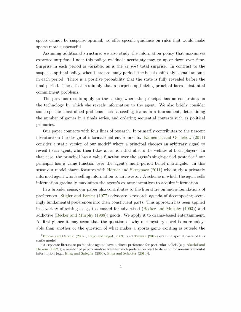
Note that suspense is experienced ex ante whereas surprise is experienced ex post. There

is another crucial distinction between the two concepts. The overall surprise depends solely

on the belief path realized. In contrast, suspense depends on the belief martingale as well

as the belief path. Recall Figure 1. The realized belief paths fully determine the surprise,

but not the suspense, generated by each match. Suspense at a given point depends on the

entire distribution of next period’s beliefs. In Figure 2, we illustrate this distribution by

adding gray tendrils that indicate what the belief would have been had the point turned

out differently. Figure 2 makes it apparent that Djokovic-Federer was a more suspenseful

match than Murray-Nadal.

As we mentioned in the introduction, we believe suspense and surprise are important

in many contexts.12 Sports fans enjoy the drama of the shifting fortunes between players.

10Neurobiological evidence suggests that, in monkeys, suspense about whether a reward will be deliveredinduces sustained activation of dopamine neurons (Fiorillo, Tobler, and Schultz (2003)).

11Kahneman and Miller (1986) offer a different conceptualization of surprise based on the notion ofendogenously generated counterfactual alternatives.

12The applicability of our model probably depends on the stakes. On the one hand, when the stakesare too low, there is little scope for suspense and surprise since the agent is not invested in the outcome.

12

Figure 2: 2011 US Open Semifinals, Suspense and SurpriseThe gray lines indicate what the belief would have been, if the point had gone the other way.

0 50 100 150 200 250 300

0.0

0.5

1.0

Point

Pro

babi

lity

of W

in

(a) Likelihood that Djokovic beats Federer

0 50 100 150 200

0.0

0.5

1.0

Point

Pro

babi

lity

of W

in

(b) Likelihood that Murray beats Nadal

Playing blackjack at the casino, a gambler knows the odds are against her but derives

pleasure from the ups and downs of the game itself. Politicos and potential voters enjoy

following the news when there is an exciting race for political office such as the 2008

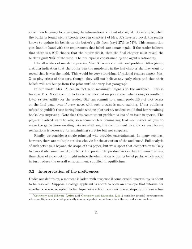
Clinton-Obama primary. Figure 3 presents data on the belief movements in each of these

settings.

For Tennis, we collected point-level data for every match played in Grand Slam tour-

naments in 2011. We focus exclusively on women’s tennis in order to have a fixed best-

out-of-three-sets structure. Each belief path is associated with a particular match. We

estimate the likelihood that a given player will win the match by assuming that the serving

player wins any given point with a fixed tournament-specific probability. This gives us, at

each point, the likelihood of a win (thick blue line) and what this likelihood would have

been had the point played out differently (thin gray tendrils). Hence, we can compute the

suspense and surprise realized in each match.

For Soccer, we collected data on over 24,000 matches played between August 2011

and July 2012 across 67 professional leagues. We exclude knockout competitions where

matches can end in overtime or penalty shootouts, so each match lasts approximately

94 minutes (inclusive of stoppage time). To parallel the binary state space in the rest

of Figure 3, we focus on the likelihood that the home team will win (vs. tie/lose). We

estimate this likelihood minute-by-minute, based on a league-specific hazard rate of goal

scoring, computed separately for the home and away teams. For each minute we also

On the other hand, if the stakes are too high, the agent will not be in the mood for entertainment. Theseconsiderations are particularly important when stakes are endogenous (e.g., in a gambling context).

13

Figure 3: Suspense and surprise from a variety of processes

Process Median Belief Path Suspense and Surprise

Tennis

0 20 40 60 80 100 120

0.0

0.5

1.0

Point

Pro

babi

lity

of W

in

0.0 0.5 1.0 1.5 2.0

0.0

1.0

2.0

Surprise

Sus

pens

e

Soccer

0 20 40 60 80 100

0.0

0.5

1.0

Minute

Pro

babi

lity

of W

in

0.0 0.5 1.0 1.5 2.0

0.0

1.0

2.0

Surprise

Sus

pens

e

Blackjack

0 100 200 300 400

0.0

0.5

1.0

Card

Pro

babi

lity

of W

in

0.0 0.5 1.0 1.5 2.0

0.0

1.0

2.0

Surprise

Sus

pens

e

Clinton-ObamaPrimary

0 100 200 300 400 500

0.0

0.5

1.0

Day

Pro

babi

lity

of W

in

0.0 0.5 1.0 1.5 2.0

0.0

1.0

2.0

Surprise

Sus

pens

e

SurpriseOptimum

0 10 20 30 40 50

0.0

0.5

1.0

Period

Pro

babi

lity

of W

in

0.0 0.5 1.0 1.5 2.0

0.0

1.0

2.0

Surprise

Sus

pens

e

SuspenseOptimum

0 10 20 30 40 50

0.0

0.5

1.0

Period

Pro

babi

lity

of W

in

0.0 0.5 1.0 1.5 2.0

0.0

1.0

2.0

Surprise

Sus

pens

e

14

estimate the beliefs that would have realized if the home team, away team, or neither team

had scored. Thus, as for tennis, we can compute the suspense and surprise generated by

each soccer match.

For Blackjack, we simulate 20,000 visits to Las Vegas. On every visit, our artificial gam-

bler begins with a budget of $100 and plays $10-hands of blackjack until he either increases

his stack to $200 or loses all his money. Each belief path is associated with a particu-

lar visit. The dealer’s behavior in blackjack is regulated and our gambler strictly follows

optimal (non-card-counting) play. Hence, following each individual card that is dealt, we

can explicitly compute the updated probability that the gambler will walk away with the

winnings rather than empty-handed. Also, we can determine what this probability would

have been for every other card that could have been dealt. This allows us to determine

the suspense and surprise realized in each visit. Moreover, we can use these simulations

to examine how a given change in casino rules would influence the distribution of suspense

and surprise. For example, we confirm that allowing doubling down and splitting, as all

Vegas casinos do, indeed increases expected suspense and surprise.13

For Clinton-Obama Primary, we depict the daily average price of a security that pays

out if Obama wins the 2008 Democratic National Convention. There is a single belief path

for this particular primary. Unlike for Tennis and Blackjack, these data do not provide

a way to estimate the distribution of next day’s beliefs. Hence, we are able to compute

realized surprise but not suspense.

For comparison we also draw 1,000 belief paths from the suspense- and surprise-optimal

martingales.

In the right panel of Figure 3, we display the scatterplot of realized suspense and

surprise for each setting.14 We identify the observation that is closest to the median level

of suspense and median level of surprise. We mark this observation with a black circle in

the right panel and depict its belief path in the left panel. Additional details about the

construction of Figure 3 are in the Online Appendix.

These examples illustrate some of the ways that belief martingales can be estimated.

13Doubling down means the gambler is allowed to increase the initial bet by $10 after his first two cardsin exchange for committing to receive exactly one more card. Splitting means that, if the first two cardshave the same value, the player can split them into two hands and wager an additional $10 for the newhand.

14We utilize the baseline specification for u(·) and normalize realized suspense and surprise across settingsby dividing by the square root of the number of periods. (As we show later, maximal suspense and surpriseare proportional to

√T .)

15

For Blackjack, it is possible to simulate the distribution of belief paths based solely on

the structure of the rules; the data generating process is known. For the Primary, we use

data from a prediction market. For Tennis and Soccer, we estimate the likelihood of the

relevant events (server will win the point, home team will score, etc.) in each period and

derive the belief path implied.15 Additionally, belief martingales might be elicited through

laboratory experiments. For instance, a researcher could pay subjects to read a mystery

novel and incentivize them to guess who the murderer is after each chapter. We hope that

in future research this range of methods will allow for construction of datasets on suspense

and surprise in a number of other contexts.

3.3 Illustrative examples

To develop basic intuition about the model, we consider a few examples where the princi-

pal’s problem can be analyzed without any mathematics.

Suppose a principal wishes to auction a single object to bidders who have independent

private values but also enjoy suspense or surprise about whether they will win the auction.

The principal must choose between the English auction and the second-price sealed-bid

auction. Conditional on standard bidding behavior, the English auction is preferable; it

reveals information about the winner slowly rather than all at once, so it gives bidders a

higher entertainment payoff.

Or, consider elimination announcements on a reality TV show. In each episode, one of

two contestants, say Scottie or Haley, gets eliminated. The host of the show calls out one of

the names, e.g., “Scottie, please step forward.” Then, she either says“You are eliminated”or

“You go through”to the person who was called. If the host always called the person who was

to be eliminated, or the person who would go through, then the outcome would be revealed

immediately when she asked Scottie to step forward. If the host chose participants without

regard to elimination, then calling Scottie to step forward would convey no information

at all. The second comment would reveal everything. To increase suspense or surprise,

the host should make the initial call partially informative. Having called Scottie forward,

the audience should believe that Scottie is now either more likely to go through or more

15Our estimation procedure for both Tennis and Soccer is admittedly crude, but it serves to illustratea method for deriving belief paths. For Tennis, if we had more data we could estimate the likelihood agiven player wins a given point conditional on the surface, the current score, the recent change in score, theplayers’ rankings, etc. Or, one could directly estimate the likelihood a given player wins the entire matchgiven these factors. Similar considerations apply to Soccer.

16

likely to be eliminated. Either policy works, as long as the audience understands how to

interpret the signal. Anecdotally, many reality TV shows seem to follow this formula.

Economists and psychologists have extensively studied why people gamble – why they

spend money in casinos. Our model gives a rationale for why people spend time in casi-

nos. The weekend’s monetary bets (a compound lottery) could be reduced to a single bet

(a simple lottery). But this would deprive the gambler of an important element of the

casino experience. Part of the fun of gambling is the suspense and surprise as the gambler

anticipates and then observes each flip of a card, spin of the wheel, or roll of the dice.16

These three examples are specific instances of a more general feature of suspense and

surprise: spoilers are bad. In other words, revealing all the information at once (as a spoiler

does) yields the absolute minimum suspense and surprise (given that all information is

revealed by the end). This feature of the preferences seems in accordance with real-world

intuitions about suspense and surprise.17

Finally, when watching a sports match between two unfamiliar teams, spectators com-

monly root for the underdog or the trailing team. Our model gives an explanation for

this kind of behavior. There is more surprise when the underdog wins. And when the

trailing team scores, we have a closer match which generates more continuation suspense

and surprise.

4 Suspense-Optimal Information Policies

In this section, we take the prior and the number of periods as given and derive the

information policy that maximizes expected suspense. As we discussed above, any plausible

utility function u(·) over suspense is strictly concave. Accordingly, this is the case we focus

on in this section.18

16Barberis (2012) considers a model where gamblers behave according to prospect theory. Casinos thenoffer dynamic gambles so as to exploit the time inconsistency induced by non-linear probability weighting.

17Christenfeld and Leavitt (2011) claim that readers in fact prefer spoilers. However, they obtain thisresult only when spoilers are announced rather than embedded within the text, which raises concerns aboutexperimenter demand effects.

18If u (·) is linear, then any information policy that is fully revealing by the end yields the same overallsuspense. If u (·) is strictly convex, revealing the state in any single period is uniquely optimal.

17

4.1 Solving the Principal’s Problem

Recall that given any belief martingale, there exists an information policy which induces it

(Lemma 1). So we can think of the principal’s choice of an information policy as equivalent

to the choice of a martingale. To simplify notation, let the aggregated variance of period

t+ 1 beliefs, given information at time t, be denoted by

σ2t ≡ E

∑ω

(µωt+1 − µωt

)2.

We can then write the principal’s problem as maximizing Eµ∑T−1

t=0 u(σ2t

).

We begin by making two observations. First, any suspense-optimal martingale will be

fully revealing by the end, i.e., the final belief µT is degenerate. To see this, take some

policy that does not always fully reveal and modify the last signal to be fully informative.

This increases σ2T−1 and leaves σ2

t unchanged at t < T − 1, raising suspense.

Second, all martingales that are fully revealing by the end yield the same expected sum

of variances, E〈π|µ0〉∑T−1

t=0 σ2t . This follows from the fact that martingale differences are

uncorrelated. For any collection of uncorrelated random variables, the sum of variances

is equal to the variance of the sum. Hence, any fully revealing policy π yields the same

E〈π|µ0〉∑T−1

t=0 σ2t as the policy that reveals the state in a single period.19 The same logic

holds, going forward, from any current belief µ at any period. We denote this residual

variance from full revelation by Ψ(µ) ≡∑

ω µω(1− µω).

We summarize these two points in the following lemma.

Lemma 2. Any suspense-maximizing information policy is fully revealing by the end. Un-

der any information policy π that is fully revealing by the end, E〈π|µ0〉∑T−1

t=0 σ2t = Ψ(µ0).

Starting from the prior, the principal can thus be thought of as having a “budget of

variance” equal to Ψ(µ0). The principal then decides how to allocate this variance across

periods so as to maximize Eµ∑

t u(σ2t ) subject to Eµ

∑t σ

2t = Ψ(µ0). By concavity of

u(·), it would be ideal to dole out variance evenly over time. Is it possible to construct an

information policy so that σ2t is equal to Ψ(µ0)/T in each period t, on every path? If so,

19Augenblick and Rabin (2012) also point out this feature of belief martingales; they use it to constructa test of Bayesian rationality. Residual variance also plays a role in insider trading models (Kyle (1985),Ostrovsky (2012)) where it captures how much of the insider’s private information has not yet been revealedto the market. This bounds the total variation in future prices which in turn places an upper bound on theinsider’s profits.

18

such a policy would be optimal. In fact, we can construct such a policy. Let

Mt ≡µ

∣∣∣∣ Ψ(µ) =T − tT

Ψ(µ0)

.

Proposition 1. Fix any strictly concave u(·). A belief martingale maximizes expected

suspense if and only if µt ∈Mt for all t. The agent’s expected suspense from such a policy

is Tu(

Ψ(µ0)T

).

Proof. A martingale µ that is fully revealing by the end has σ2t constant across t if and

only if Ψ(µt) = T−tT Ψ(µ0), or in other words µt ∈Mt, for all t. We are going to show that

in fact there exists a martingale µ with µt ∈ Mt for all t (which therefore has constant

σ2t ). Then by Lemma 1, we know that there exists a policy π s.t. 〈π | µ0〉 = µ. It follows

that µ is optimal, proving the sufficiency part of the Proposition. Any martingale with

non-constant σ2t gives a lower payoff, establishing necessity.

In general, given any sequence of sets (Xt), there exists a martingale µ s.t. Supp (µt) ⊂Xt ∀t if Xt ⊂ conv (Xt+1) ∀t. Therefore, it remains to show that Mt ⊂ conv (Mt+1) ∀t. By

definition of Ψ (·), for any k ≥ 0 we have conv (µ | Ψ (µ) = k) = µ | Ψ (µ) ≥ k. Hence,

Mt =µ | Ψ (µ) = T−t

T Ψ (µ0)⊂µ | Ψ (µ) ≥ T−(t+1)

T Ψ (µ0)

= conv (Mt+1).

This proposition provides a recipe for constructing a suspense-optimal information pol-

icy. At the outset, the belief µ0 is contained in M0. In each period t, given µt ∈ Mt, the

principal chooses a signal that induces a distribution of beliefs whose support is contained

in the set Mt+1. Any distribution of beliefs µt+1 can be induced by some signal so long as

Eµt+1 [µt+1] = µt; this includes distributions with support in Mt+1, as shown in the proof

of Proposition 1. In particular, given µt+1, let π (s | ω) = µωs µt+1(µs)µωt

. By Bayes’ Rule, this

signal induces µt+1.

There is a natural geometric interpretation of the set Mt which sheds further light

on the structure of suspense-optimal information policies. The set Mt is defined as those

beliefs with residual variance T−tT Ψ(µ0). Following some simple algebra, we can equivalently

characterize each Mt as a “circle” (a hypersphere) centered at the uniform belief. Denoting

the uniform belief by µ∗ ≡(

1|Ω| , ...,

1|Ω|

), we can write Mt as

Mt =

µ

∣∣∣∣ |µ− µ∗|2 = |µ0 − µ∗|2 +t

TΨ(µ0)

where |µ− µ∗|2 =

∑ω(µω − µω∗ )2 denotes the square of the Euclidean distance between µ

19

and µ∗. The uniform belief µ∗ has the highest residual variance of all beliefs, and residual

variance falls off with the square of the distance from µ∗. The residual variance of beliefs in

Mt falls linearly in t, and hence beliefs lie on circles whose radius-squared increases linearly

over time. At time T , the circle has the maximum radius and intersects ∆(Ω) only at

degenerate beliefs. Figure 4 illustrates this geometric characterization of suspense-optimal

information policies.

Figure 4: The path of beliefs with Ω = 0, 1, 2

The triangle represents ∆(Ω), the two-dimensional space of possible beliefs. The Mt sets are circlescentered on the uniform belief µ∗, intersected with the triangle ∆(Ω). The belief begins at µ0; inthis picture µ0 is at µ∗. The belief µt at time t will be in Mt. Given current belief µt ∈ Mt, anydistribution µt+1 over next-period beliefs with mean µt and support contained in Mt+1 is consistentwith a suspense-maximizing policy. At time T the uncertainty is resolved, so µT will be on a cornerof the triangle.

Below we summarize some of the key qualitative features of suspense-optimal informa-

tion revelation.

The state is revealed in the last period, and not before. As long as the prior is not

degenerate, the residual variance is positive at any time t < T . In particular, the

20

residual variance at time t is T−tT Ψ(µ0).

Uncertainty declines over time. Uncertainty, as measured by the residual variance,

declines linearly over time from Ψ(µ0) to 0.

Realized suspense is deterministic. There is no ex post variation in suspense. Al-

though the path of beliefs is random, the agent’s suspense is the same across every

realization. It is always exactly Tu(Ψ(µ0)/T ).

Suspense is constant over time. The variance σ2t in each period t is Ψ(µ0)/T . So the

agent’s experienced suspense is u(Ψ(µ0)/T ) in each period.

The prior that maximizes suspense is the uniform belief. Total suspense is Tu(Ψ(µ0)/T ).

The budget of variance Ψ(µ0) is increasing in the proximity of µ0 to µ∗; Ψ(µ0) is max-

imized at µ0 = µ∗.

The level of suspense increases in the number of periods T . It is immediate from

the outset that suspense must be weakly increasing in T – any signals that can be

sent over the course of T periods can also be sent in the first T periods of a longer

game. In fact, the suspense Tu(Ψ(µ0)/T ) is strictly increasing in T . For u(x) = xγ

with 0 < γ < 1, for instance, total suspense is proportional to T 1−γ .

Suspense-optimal information policies are independent of the stage utility function.

Under any concave u(·), any optimal policy induces beliefs in Mt. The expression for

Mt is independent of u(·).

4.2 Illustration of Suspense-Optimal Policies

4.2.1 Two states

We first illustrate these policies in the case of a binary state space Ω = A,B. In a

sporting event, will team A or team B win? In a mystery novel, is the main character

guilty or not? In this case, each set Mt consists of just two points. This leads to a unique

suspense maximizing belief martingale, depicted in Figure 5.

The suspense-optimal policy gives rise to the following dynamics. At period t the belief

µt ≡ Pr(A) is either a high value Ht >12 or a low value Lt = 1−Ht.

20 In each period, one

of two things happens. With high probability the agent observes additional confirmation

20In this binary case we abuse notation by associating the belief with the probability of one of the states.

21

Figure 5: The suspense-optimal belief martingale with 2 states

1 2 T1 Tt

0.2

0.4

0.6

0.8

1.0Μ

Ht

Lt

This picture depicts the case where µ0 = 12 . The belief at time t will be either Ht >

12 or Lt <

12 .

The probability of a plot twist (which takes beliefs from Ht to Lt+1 or from Lt to Ht+1) declinesover time.

– the high belief Ht moves to a slightly higher belief Ht+1, or the low belief Lt moves to

Lt+1. With a smaller probability, there is a plot twist. In the event of a plot twist, beliefs

jump from the high path to the low one, or vice versa. As time passes, plot twists become

larger but less likely.21 If we consider a limit as T goes to infinity, the arrival of plot twists

approaches a Poisson process with an arrival rate that decreases over time.22

In the context of a mystery novel, these dynamics imply the following familiar plot

structure. At each point in the book, the reader thinks that the weight of evidence either

suggests that the protagonist accused of murder is guilty or is innocent. But in any given

chapter, there is a chance of a plot twist that reverses the reader’s beliefs. As the book

21 We can solve for Ht and Lt explicitly as

Ht =1

2+

√(µ0 −

1

2

)2

+t

Tµ0 (1− µ0), Lt =

1

2−

√(µ0 −

1

2

)2

+t

Tµ0 (1− µ0).

The probability of a plot twist is1

2− 1

2

√(µ0 − 1

2)2 + t−1

Tµ0(1− µ0)√

(µ0 − 12)2 + t

Tµ0(1− µ0)

.

22To derive the limit, take T to infinity and rescale time to s = t/T . This yields a Poisson process with

plot twist arrival intensity of µ0(1−µ0)1−4(1−s)µ0(1−µ0)

.

22

continues along, plot twists become less likely but more dramatic.

In the context of sports, optimal dynamics could be induced by the following set of

rules. We declare the winner to be the last team to score. Moreover, scoring becomes more

difficult as the game progresses (e.g., the goal shrinks over time). The former ensures that

uncertainty declines over time while the latter generates a decreasing arrival rate of plot

twists. (In this context, plot twists are lead changes).

Note that existing rules of most sports cannot be suspense optimal. In soccer, for

example, the probability that the leading team will win depends not only on the period of

the game, but also on whether it is a tight game or a blowout. Moreover, the team that

is behind can come back to tie up the game, in which case uncertainty will have increased

rather than decreased over time.

To conclude the discussion of binary states, we note the following qualitative points

that apply in this case.

Beliefs can jump by a large amount in a single period. In each period, either be-

liefs are confirmed or there is a plot twist. A plot twist takes beliefs from µt to

something further away than 1− µt.

Belief paths are smooth with rare discrete jumps when there are many periods.

Beliefs move along the increasing Ht or decreasing Lt curves with occasional plot

twists when beliefs jump from one curve to the other. In the limit as T gets large,

the expected number of total plot twists stays small. Expected absolute variation∑T−1t=0 |µt+1 − µt| converges to a finite value as T goes to infinity.23

4.2.2 Three or more states

With more than two possible outcomes, there is additional flexibility in the design of a

suspense-maximizing martingale. Say that there is a mystery novel with three suspects,

and we currently believe A to be the most likely murderer. In the next chapter we will see

a clue (a signal) which alters our beliefs, either providing further evidence of A’s guilt or

pointing to B or C as suspects. It may be the case that there are three possible clues we

can see, or five, or fifty. The only restriction is that after observing the clue, our belief has

the right amount of uncertainty as measured by residual variance.

23In the limit as T →∞, the expected absolute variation converges to 2 minµ0, 1− µ0.

23

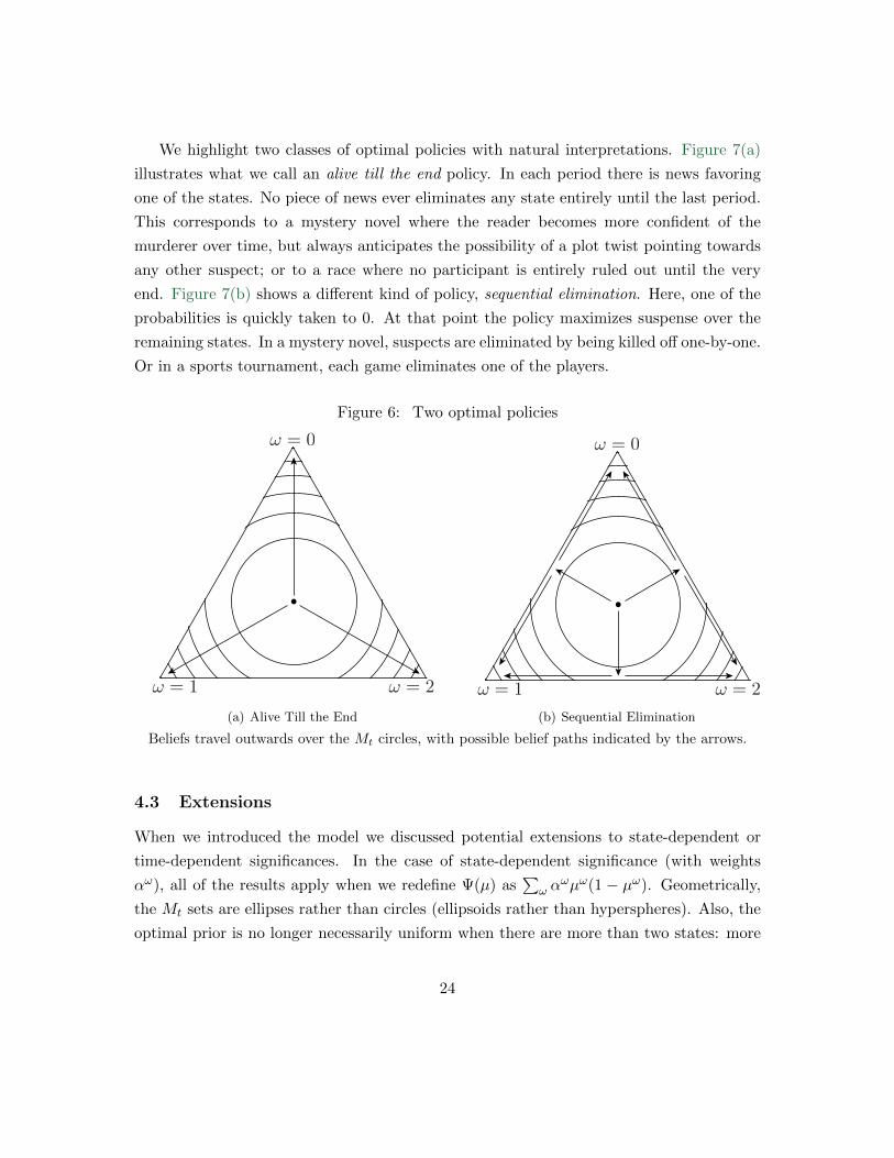
We highlight two classes of optimal policies with natural interpretations. Figure 7(a)

illustrates what we call an alive till the end policy. In each period there is news favoring

one of the states. No piece of news ever eliminates any state entirely until the last period.

This corresponds to a mystery novel where the reader becomes more confident of the

murderer over time, but always anticipates the possibility of a plot twist pointing towards

any other suspect; or to a race where no participant is entirely ruled out until the very

end. Figure 7(b) shows a different kind of policy, sequential elimination. Here, one of the

probabilities is quickly taken to 0. At that point the policy maximizes suspense over the

remaining states. In a mystery novel, suspects are eliminated by being killed off one-by-one.

Or in a sports tournament, each game eliminates one of the players.

Figure 6: Two optimal policies

(a) Alive Till the End

(b) Sequential Elimination

Beliefs travel outwards over the Mt circles, with possible belief paths indicated by the arrows.

4.3 Extensions

When we introduced the model we discussed potential extensions to state-dependent or

time-dependent significances. In the case of state-dependent significance (with weights

αω), all of the results apply when we redefine Ψ(µ) as∑

ω αωµω(1 − µω). Geometrically,

the Mt sets are ellipses rather than circles (ellipsoids rather than hyperspheres). Also, the

optimal prior is no longer necessarily uniform when there are more than two states: more

24

significant states are given priors closer to 12 . Sufficiently insignificant states may be given

a prior of 0, and as the significance of one state begins to dominate all others the prior on

that state goes to 12 .

An alternative extension is a setting where the principal chooses αω’s and µ0.24 (For

example, a sports league may be able to influence the market share across teams, or the

novelist chooses how much reader empathy to generate for each character.) In this case,

the principal’s choice is optimal if and only if µω0 = 12 for each state with αω > 0.25 This

means that there are two basic ways to maximize suspense. One way is to have only two

states of interest, with 50/50 odds between those two. Good versus evil, Democrat versus

Republican, Barcelona vs. Real Madrid. Alternatively, there may be a single state of inter-

est, realized with probability 50%. The reader cares only about whether the protagonist is

found innocent or guilty. Conditional on the protagonist’s innocence, any of the irrelevant

characters may be the murderer with any probabilities.

In the case of time-dependent significances (with weights βt), it is no longer optimal to

divide suspense evenly over time. Instead, more important periods are made to be more

suspenseful. For example, in the baseline specification for u(·), we set σt proportional to

βt.

5 Surprise-Optimal Information Policies

Solving for the surprise-optimal martingale is difficult in general and, in contrast to the case

of suspense, sensitive to the choice of u(·). So in this section we restrict attention to binary

states Ω = A,B and the baseline specification where surprise in period t equals |µt−µt−1|with µt ≡ Pr(A).26 We derive an exact characterization of optimal belief martingales for

very small T , and discuss properties of the solution for large T .27

Let WT (µ) be the value function of the surprise maximization problem, where T is the

number of periods remaining and µ is the current belief. We can express the value function

24Utility increases in each αω, so to make this problem well-posed we assume that the principal isconstrained by a fixed sum of significances

∑ω α

ω.25Proof of this and other claims from this subsection are in the Online Appendix.26Recall that under the baseline specification, surprise in period t is the Euclidean distance between the

belief vectors in periods t and t− 1. To avoid introducing a nuisance term, however, in this section we setsurprise in period t to be the Euclidean distance between the scalars µt and µt−1. This amounts to scalingall surprise payoffs by 1√

2.

27In the Online Appendix, we discuss how some features of the surprise optimum change if we departfrom the baseline specification.

25

recursively by setting W0(µ) ≡ 0, and

WT (µ) = maxµ′∈∆(∆(Ω))

Eµ′[∣∣µ′ − µ∣∣+WT−1(µ′)

]s.t. Eµ′

[µ′]

= µ.

The single-period problem above can always be solved by some µ′ with binary support.28

That is, for any current belief, there is a surprise-maximizing martingale such that next

period’s belief is either some µl or µh ≥ µl.The solution can be derived by working backwards from the last period. In the final

period, it is optimal to fully reveal from any prior: µl = 0 and µh = 1. This yields a value

function of W1(µ) = 2µ(1− µ).

With two periods remaining, it is optimal to set µl = µ− 14 and µh = µ+ 1

4 , as long as

µ ∈ [14 ,

34 ]. Therefore if µ0 = 1

2 and T = 2, the surprise-optimal martingale induces beliefs

µl = 14 or µh = 3

4 in period 1, and then fully reveals the state in the second period. The

details of this and the next derivation are in Appendix A.1.

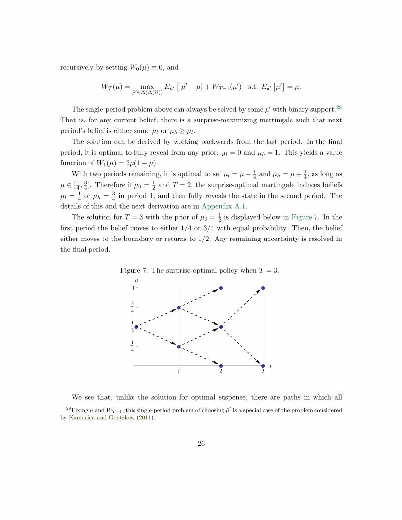
The solution for T = 3 with the prior of µ0 = 12 is displayed below in Figure 7. In the

first period the belief moves to either 1/4 or 3/4 with equal probability. Then, the belief

either moves to the boundary or returns to 1/2. Any remaining uncertainty is resolved in

the final period.

Figure 7: The surprise-optimal policy when T = 3.

1 2 3t

14

12

34

1Μ

We see that, unlike the solution for optimal suspense, there are paths in which all

28Fixing µ and WT−1, this single-period problem of choosing µ′ is a special case of the problem consideredby Kamenica and Gentzkow (2011).

26

uncertainty is resolved before the final period T. These paths have lower overall surprise

than the paths that resolve only at the end. But the optimal information policy accepts a

positive probability of early resolution in return for a chance to move beliefs back to the

interior and set the stage for later surprises. Also unlike the suspense solution, uncertainty

can both increase or decrease over time. Beliefs may move towards an edge, or back towards12 . In the suspense-optimal martingale, uncertainty only increases.

These features underscore the commitment problem facing a surprise-maximizing prin-

cipal. The surprise-optimal martingale has paths that generate very little surprise. In order

to implement the optimal policy, the principal requires the commitment power to follow

such paths. Otherwise, he is tempted to prune such paths and choose a path with maximal

surprise. The agent would expect this deviation and the chosen path would no longer be

surprising.29 In contrast, maximizing suspense does not involve this form of commitment

because the suspense-optimal information policy yields equal suspense across all realized

paths.

This importance of commitment sheds some light on the phenomenon of dedicated

sports fans. It may seem tempting to record a game and let others tell you whether it was

exciting before you decide whether to watch it.30 However, such a strategy is self-defeating:

the very knowledge that the game was exciting reduces its excitement. Similarly, if ESPN

Classic shows only those games with comeback victories, the audience would never be

surprised at the comeback. To make the comebacks surprising, ESPN Classic would have

to show some games in which one team took a commanding early lead and never looked

back.

For arbitrary T , it is difficult to analytically solve for surprise-optimal belief martingales.

The properties of the value function WT (µ) in the limit as T goes to infinity, however, have

previously been studied by Mertens and Zamir (1977). Their interest in this limiting

variation of a bounded martingale arose in the study of repeated games with asymmetric

information.31

29Without commitment, all paths (including ones where the belief moves monotonically to a boundary)must generate the same surprise in equilibrium. Hence the principal’s payoff cannot be greater than if allinformation is revealed at once. This echoes Geanakoplos’s (1996) result about the Hangman’s Paradox.

30The web site http://ShouldIWatch.com, for example, provides this information.31De Meyer (1998) extends their results to the more general Lq variation, i.e., he considers the problem

of maximizing E[∑T−1

t=0 (E|µk+1 − µk|q)1q

]. Under binary states and the baseline specification, this is our

surprise problem if q = 1 and our suspense problem if q = 2. De Meyer searches for the limit of the Lq valuefunction divided by

√T , as T goes to infinity. He finds that for q ∈ [1, 2), this limit is constant in q and

is equal to φ(µ), as given in Proposition 2 for q = 1. For q > 2, de Meyer finds that the limit approaches

27

Proposition 2 (Mertens and Zamir (1977), Equation (4.22)). For any µ,

limT→∞

WT (µ)√T

= φ(µ),

where φ(µ) is the pdf of the standard normal distribution evaluated at its µth-quantile:

φ(µ) =1√2πe−

12x2µ, with xµ defined by

∫ xµ

−∞

1√2πe−

12x2dx = µ.

In particular,√Tφ(µ)− α ≤ WT (µ) ≤

√Tφ(µ) + α for some constant α > 0 independent

of µ and T .

The fact that the ex ante surprise payoff – i.e., the expected absolute variation – goes

to infinity tells us that paths are “spiky” rather than smooth as T gets large. Recall that

in the suspense optimal martingale, expected absolute variation was bounded in T .

Another difference between optimal surprise and suspense is the range of possible belief

changes in a given period. In each period of the suspense problem, there is a chance of a

twist that leads to a large shift in beliefs. In the surprise problem, however, beliefs move

up or down only a small amount in periods when there is a lot of time remaining.

Proposition 3. For all ε > 0, if T − t is sufficiently large then for any belief path in the

support of any surprise-optimal martingale, |µt+1 − µt| < ε.

The proof, in Appendix A.2, builds on Proposition 2. We can now summarize some

qualitative features of surprise-optimal information revelation.

The state is fully revealed, possibly before the final period. Any time the belief

at T − 2 is below 14 or above 3

4 , for instance, there is a chance of full revelation

at period T − 1.

Uncertainty may increase or decrease over time. Beliefs often move toward µ = 12 .

With sufficiently many periods remaining, residual uncertainty in the next period can

always either increase or decrease (except in the special case of µt = 12).

infinity for any µ ∈ (0, 1). However, de Meyer incorrectly suggests that the methods of Mertens and Zamircan be used to show that the value function for q = 2 will be identical to that for q < 2. In fact, oursolution to the suspense problem with binary states and the baseline specification shows this to be false.The limiting value function is

√µ(1− µ) rather than φ(µ).

28

Realized surprise is stochastic. In an optimal martingale there are low surprise paths

(e.g., ones in which beliefs move monotonically to an edge) or high surprise paths

(with a lot of movement up and down).

Surprise varies over time. Both realized and expected surprise can vary over time.

Consider T = 2 where µ0 = 12 , µ1 ∈ 1

4 ,34, and µ2 ∈ 0, 1. On a particular

belief path, say (12 ,

14 , 1), realized surprise in period 1 is different from realized sur-

prise in period 2. Moreover, from the ex ante perspective, the expected surprise in

period 1 is 14 while the expected surprise in period 2 is 3

8 .

The prior that maximizes surprise is the uniform belief. We show that for T ≤ 3,

surprise is maximized at the uniform prior. We conjecture that this holds for all T .

Proposition 2 shows that surprise is maximized at the uniform prior in the limit as

T →∞.

The level of surprise increases in the number of periods T . While we do not have

a general expression for surprise as a function of T , we know that in the limit surprise

increases proportionally with√T . It is obvious that surprise is weakly increasing in

T .

Beliefs change little when there are many periods remaining. By Proposition 3,

|µt+1 − µt| is small when T − t is large.

Belief paths are spiky when there are many periods. Expected absolute variation,

which is equal to the surprise value function, goes to infinity as T gets large.

Surprise-optimal information policies depend on the stage utility function. In the

Online Appendix, we consider alternative u(·) functions. For very concave u(·), the

surprise-optimal policy can be non-fully revealing by the end. For convex u(·), the

surprise-optimal prior can be non-uniform.

6 Comparing Suspense and Surprise

As the two preceding sections reveal, suspense-optimal and surprise-optimal belief martin-

gales are qualitatively different. Another way to appreciate these differences is to consider

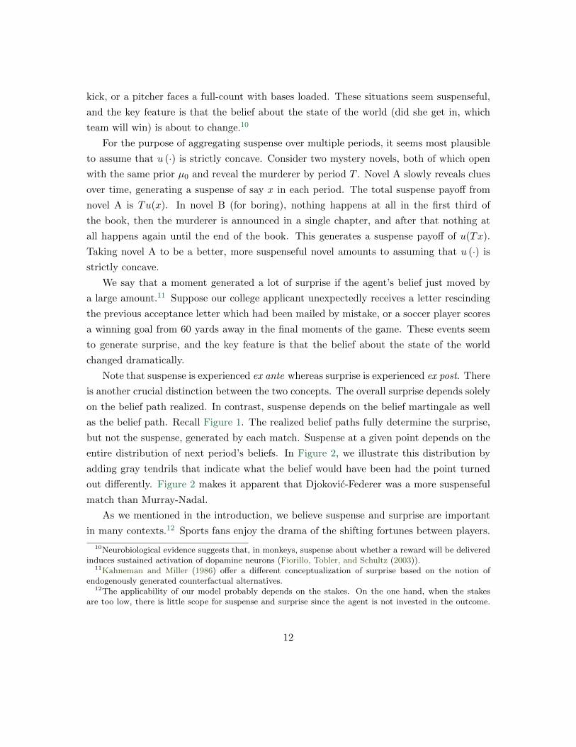
sample belief paths drawn from a suspense-optimal and a surprise-optimal martingale, as

29

shown in Figure 8. Here we show three representative belief paths for each of the two pro-

cesses: a path at the 25th percentile of suspense and surprise from the simulations of Fig-

ure 3, at the median, and at the 75th percentile. The suspense paths reveal the distinctive

plot-twist structure whereas the surprise paths show the spiky nature of surprise-optimal

martingales.

Figure 8: Sample suspense- and surprise-optimal belief paths.

Suspense Surprise

25thPercentile

0 10 20 30 40 50

0.0

0.5

1.0

Period

Pro

babi

lity

of W

in

0 10 20 30 40 50

0.0

0.5

1.0

Period

Pro

babi

lity

of W

in

50thPercentile

0 10 20 30 40 50

0.0

0.5

1.0

Period

Pro

babi

lity

of W

in

0 10 20 30 40 50

0.0

0.5

1.0

Period

Pro

babi

lity

of W

in

75thPercentile

0 10 20 30 40 50

0.0

0.5

1.0

Period

Pro

babi

lity

of W

in

0 10 20 30 40 50

0.0

0.5

1.0

Period

Pro

babi

lity

of W

in

While no existing sport would induce the exact distributions of belief paths we derive,

we can think of soccer and basketball as representing extreme examples of sports with the

qualitative features of optimum suspense and surprise. In any given minute of a soccer

game it is very likely that nothing consequential happens. Whichever team is currently

ahead becomes slightly more likely to win (since less time remains). There is a small chance

that a team scores a goal, however, which would have a huge impact on beliefs. So (as

Figure 3 illustrates), belief paths in soccer are smooth, with few rare jumps. This sustained

small probability of large belief shifts makes soccer a very suspenseful game. In basketball,

points are scored every minute. With every possession, a team becomes slightly more likely

30

to win if it scores and slightly less likely to win if it does not. But no single possession can

have a very large impact on beliefs, at least not until the final minutes of the game. Belief

paths are spiky, with a high frequency of small jumps up and down; basketball is a game

with lots of surprise.

The distinction between suspense-optimal and surprise-optimal martingales somewhat

clashes with an intuition that more suspenseful events also generate more surprise. This

intuition is indeed valid in the following two senses. First, given a martingale, belief

paths with high realized suspense tend to have high realized surprise; this can be seen

in the right column of Figure 3. Moreover, the ex ante suspense and surprise are highly

correlated across martingales generated by “random” information policies. Specifically,

suppose T = 10, Ω = L,R, and µ0 = 12 . In periods 1 through 9, a signal realization l

or r is observed. When the true state is ω, the signal πω,t at period t is l with probability

ρω,t and r with probability 1− ρω,t. The values of ρω,t are drawn iid uniformly from [0, 1]

for each ω and t. The state is revealed in period 10. Figure 9 depicts a scatterplot of

ex ante suspense and surprise of 250 such random policies; it is clear that policies that

generate more suspense also tend to generate more surprise. Note that these policies are

history-independent in the sense that the signal sent at period t depends only on t and

not on µt. The figure also shows the numerically derived production possibilities set for

suspense and surprise over all fully revealing policies. As this set reveals, the suspense-

optimal martingale does not generate much surprise while the surprise-optimal martingale

only reduces suspense a little below its maximum. This suggests that maximizing a convex

combination of suspense and surprise is likely to lead to belief paths that resemble the

surprise optimum.

7 Constrained Information Policies

In practice there are often institutional restrictions which impose constraints on the infor-

mation the principal can release over time. Recall that we formalize these situations as the

principal’s choosing (π, µ0, T ) ∈ P so as to maximize expected suspense or surprise. In this

section we will study the nature of the constraint set and the constrained-optimal policies

in some specific examples. Throughout this section, we impose the baseline specification

for u(·).

31

Figure 9: The Surprise-Suspense frontier

Surprise

Suspense

7.1 Tournament Seeding

Consider the problem of designing an elimination tournament to maximize spectator in-

terest. Elimination tournaments begin by “seeding” teams into a bracket. The traditional

seeding pits stronger teams against weaker teams in early rounds thereby amplifying their

relative advantage. We analyze the effect of this choice on the suspense and surprise gener-

ated by the tournament. The tradeoff is clear: by further disadvantaging the weaker team,

the traditional seeding reduces the chance of an upset but increases the drama when an

upset does occur.

The simplest example of tournament seeding occurs when there are three teams. Two

teams play in a first round and the winner plays the remaining team in the final. This

remaining team is said to have the first-round “bye.” Which team should have the bye?

Formally, the state of the world ω is identified with the team that wins the overall

tournament, so ω ∈ 1, 2, 3. Assume that the probability that a team wins an individual

contest is determined by the difference in the ranking of the two teams. Let p > 12 denote

the probability that a team defeats the team that is just below it in the ranking, e.g. that

i beats team i + 1; and let q > p denote the probability that team 1 defeats team 3. The

principal chooses which team will be awarded the bye. This determines the prior as well as

the sequence of signals. For example, team 1’s prior probability of winning the tournament

is p2 + (1− p)q if team 1 has the bye and pq if team 2 has the bye. This choice of seeding

implies that first it will be revealed whether team 2 or team 3 has lost, and then it will be

32

revealed which of the remaining teams has won. Figure 10 illustrates the belief paths for

each of the possible tournament structures.

(a) Team 1 has the bye (b) Team 2 has the bye. (c) Team 3 has the bye.

Figure 10: Beliefs paths for alternate seedings.

Notice that one of the shortcomings of the traditional seeding in which the strongest

team has the bye is that it has low residual uncertainty. In fact, for any p and q, straightfor-

ward algebra shows that this traditional seeding generates the least surprise; it is optimal

to give the third team the bye. In the case of suspense, the conclusions are less clear cut

but for many reasonable parameters this same ordering holds.

There are of course many other reasons for the traditional seeding which favors the

stronger teams. Incentives are an important consideration: teams that perform well from

tournament to tournament improve their rankings and are rewarded with better seedings

in subsequent tournaments. Our analysis suggests that optimizing the tournament seeding

for its incentive properties can have a cost in short-run suspense and surprise.

7.2 Number of Games in a Playoff Series

Each round of the NBA playoffs consists of a best-of-seven series. Major League Baseball

playoffs use best-of-five series for early rounds, and best-of-seven for later rounds. In the

NFL playoffs, each elimination round consists of a single game. Of course the length of the

series is partly determined by logistical considerations, but it also influences the suspense

and surprise. On the one hand, having more games leads to slower information revelation,

increasing suspense and surprise. On the other hand, in a long series the team which is

better on average is more likely to eventually win, and this reduces both suspense and

surprise. If a team wins 60% of the matches, there is much more uncertainty over the

33

outcome of a single match than over the outcome of a best-of-seven series, or a best-of-

seventeen one. With less uncertainty there is less scope for suspense and surprise.

Formally, consider two teams playing a sequence of games against each other. The

favored team has an independent probability p > .5 of winning any given game. The

organizer chooses some odd number T and declares that the winner of the series is the first

team to win T+12 out of T total games. The organizer chooses T to maximize suspense or

surprise.

As we show in Appendix B, suspense and surprise are proportional to one another for

any choice of T . Therefore, for this class of constrained problems, maximizing suspense is

equivalent to maximizing surprise.

In Table 1 we display the suspense- and surprise-maximizing series length T ∗ as a

function of p. As the table shows, the maximizing series length is increasing in the proximity

of p to 12 . The intuition behind this is simple. When neither team is much better than the

other, the cost of a large T becomes small (µ0 does not move far from µ∗) while the benefit

of releasing information slowly remains.

Table 1: Suspense- and Surprise-Maximizing Length of a Playoff Series

p.9 .8 .75 .7 .65 .6 .55 .51

T ∗ 1 1 3 5 11 23 99 2499

7.3 Sequential Contests

The order of sequential primary elections may affect which political candidate is ultimately

chosen as a party’s nominee for President (Knight and Schiff (2007)). If voters in late

states converge around early winners, then it surely matters whether Iowa goes first, or

New Hampshire, or Florida. As a number of researchers have analyzed, e.g. Hummel

and Holden (2012), political parties may want to choose the order of primaries so as to

maximize the expected quality of a nominee.

We now pose a different question: in what order should the states vote if the goal is

to maximize the suspense or surprise of the race? A more exciting primary season may

elicit more attention from citizens, yielding a more engaged and informed electorate. In

order to highlight the relevant mechanisms, our analysis here will assume that the order of

34

primaries does not affect the likelihood any given candidate wins.

We model a primary campaign as follows. Two candidates, A and B, compete against

each other in a series of winner-take-all state primary elections. State i has ni delegates

and will be won by candidate A with probability pi. The probability A wins each state is

independent. CandidateA wins the nomination if and only if she gets at least n∗ ∈ [0,∑

i ni]

delegates.

Early states are sure to have a small but positive impact on beliefs about the nominee,

whereas late states have some chance of being extremely important and some chance of

having zero impact. Perhaps smaller or more partisan states should go first, so that infor-

mation about the nominee is revealed as slowly as possible. Or should large swing states

go first, to guarantee that these potentially exciting votes don’t take place after a nominee

has already been chosen?

Remarkably, for any distribution of delegates ni, for any set of probabilities pi, for any

cutoff n∗, the order of the primaries has no effect on expected suspense or surprise.32 Small

or large states, partisan or swing states – they may go in any order.

This neutrality result applies not only to political primaries but to many other settings

where a pair of players engage in sequential contests. For instance, in a televised game show,

players compete in a variety of tasks with different amounts of points at stake. Family Feud

doubles and then triples the points awarded in later rounds. Our results imply that this

leads to no more total excitement than if the high stakes rounds were at the beginning.

Likewise, in a typical best-of-seven sports series one advantaged team will be scheduled to

play four home games and three away games. We find that there is an equal amount of

suspense and surprise in the 2-3-2 format of the NBA Finals (two home, three away, then

two home games) as in the 2-2-1-1-1 format of the earlier NBA playoff rounds.

8 Conclusion

Our analysis is predicated on the assumption that people value suspense (variance of next

period’s beliefs) or surprise (movements in beliefs). We derive implications of this assump-

tion, focusing on the optimal way to release information over time.

One way to test our model would be to examine whether the information policies we

identify indeed attract a greater audience than other policies. More generally, a dataset

32Proof is in Appendix B.

35

that combines information about revealed preference with estimates of belief dynamics

would allow us to directly examine what aspects of belief dynamics generate entertainment

utility.

We have already discussed various ways one can estimate belief dynamics: (i) relying

on the explicit structure of the data generating process, (ii) using prediction markets, (iii)

estimating probabilities in each period based on outcomes of many matches, or (iv) eliciting

beliefs through incentivized laboratory experiments. In principle, it should be possible

to complement such data with measures of revealed preference. TV ratings would reveal

whether a show becomes more popular when previous episodes generate more suspense and

surprise. Or, detailed data collected by The Nielsen Company could be used to examine

whether the preferences we postulate explain channel-switching behavior during a sports

game. Whether suspense or surprise or some other aspects of belief dynamics drive demand

for non-instrumental information is fundamentally an empirical question, one which we

hope will be addressed by future research.

36

A Surprise-Optimal Policies

A.1 Surprise for T ≤ 3

Let the function fT be defined by

fT (µ′;µ) ≡ |µ′ − µ|+WT−1(µ′).

The notation f ′T (µ′;µ) will indicate the derivative with respect to the first component.

The recursive problem of maximizing surprise in a given period, starting from belief µt

at time t, can be written as

WT−t(µt) = maxµl≤µh

pfT−t(µh;µt) + (1− p)fT−t(µl;µt) (1)

where p is the probability given by pµh + (1 − p)µl = µt. Without loss of generality,

µl ≤ µ ≤ µh.

We set W0 to be identically 0, and so for any prior µ0 in the one-period problem T = 1

it is optimal to set µl = 0 and µh = 1 so that p = µ0 and the maximized value is

W1(µ0) = 2µ0(1− µ0).

Consider now the problem for T > 1, starting at period 0 (which can be embedded

as the last T periods of a longer problem). We can derive two first-order conditions for

optimality of the posteriors (µl, µh), holding the prior µ0 constant.33 First, consider moving

the pair (µl, µh) in the direction d(µl, µh) = (1,−1−pp ), i.e., moving the posteriors toward

one another along the line that keeps p, the probability of µh constant. The derivative of

the objective function in this direction is the inner product

d(µl, µh) ·((1− p)f ′T (µl;µ0), pf ′T (µh;µ0)

).

At an optimum this derivative must be non-positive, and equal to zero in the case of an

interior optimum, i.e.

f ′T (µl;µ0)− f ′T (µh;µ0) ≤ 0 (2)

33The objective function is not differentiable when, say, µh = µ0, but it is straightforward to show thatreleasing zero information is never optimal. The differentiability of WT−1 will be verified directly.

37

with equality when 0 < µl < µh < 1. Expanding the derivatives of fT (·), this translates to

d

dµlWT−1(µl)−

d

dµhWT−1(µh) ≤ 2 (3)

with equality in the interior. This condition illustrates the tradeoff in determining whether

to reveal more informative signals, increasing current surprise while decreasing the “stock”

of future surprises.

To derive an additional first-order condition, consider moving µl closer to µ0, holding

µh constant. The derivative of the objective function in this direction is

dp

dµl[fT (µh;µ0)− fT (µl;µ0)] + (1− p)dfT

dµl(µl;µ0)

which must be non-positive at an optimum and equal to zero when µl > 0. Substituting

(1− p) =µh − µtµh − µl

anddp

dµl=

µt − µh(µh − µl)2

and re-arranging, we obtain

df

dµl(µl;µ0) ≤ fT (µh;µ0)− fT (µl;µ0)

µh − µl

or, directly in terms of p and WT−1,

d

dµlWT−1(µl)−

WT−1(µh)−WT−1(µl)

µh − µl≤ 2(1− p) (4)

with equality when µl is interior. This condition connects the marginal gain in continuation

value at µl with the “average” continuation value. According to the condition, the larger

the difference between these two measures, the larger should be the probability (1− p) of

µl.

With these two conditions we can solve the surprise problems for T = 2 and T = 3.

First, recall that W1(µ) = 2µ(1 − µ), so that W ′1(µ) = 2 − 4µ. Then, to solve to problem

for T = 2 we use Equation 3 to derive 2 − 4µl − (1 − 4µh) = 2 or µh − µl = 1/2 at an

interior optimum. Substituting this equation into Equation 4 yields, after some algebra,

38

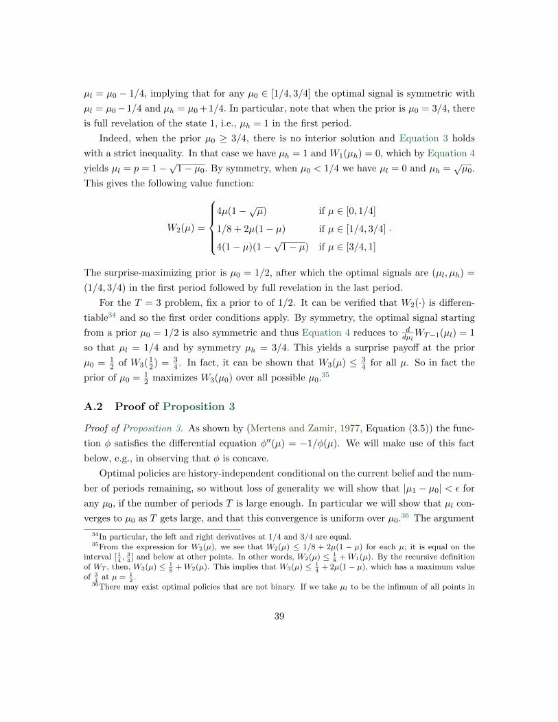
µl = µ0 − 1/4, implying that for any µ0 ∈ [1/4, 3/4] the optimal signal is symmetric with

µl = µ0−1/4 and µh = µ0 + 1/4. In particular, note that when the prior is µ0 = 3/4, there

is full revelation of the state 1, i.e., µh = 1 in the first period.

Indeed, when the prior µ0 ≥ 3/4, there is no interior solution and Equation 3 holds

with a strict inequality. In that case we have µh = 1 and W1(µh) = 0, which by Equation 4

yields µl = p = 1−√

1− µ0. By symmetry, when µ0 < 1/4 we have µl = 0 and µh =√µ0.

This gives the following value function:

W2(µ) =

4µ(1−√µ) if µ ∈ [0, 1/4]

1/8 + 2µ(1− µ) if µ ∈ [1/4, 3/4]

4(1− µ)(1−√

1− µ) if µ ∈ [3/4, 1]

.

The surprise-maximizing prior is µ0 = 1/2, after which the optimal signals are (µl, µh) =

(1/4, 3/4) in the first period followed by full revelation in the last period.

For the T = 3 problem, fix a prior to of 1/2. It can be verified that W2(·) is differen-

tiable34 and so the first order conditions apply. By symmetry, the optimal signal starting

from a prior µ0 = 1/2 is also symmetric and thus Equation 4 reduces to ddµlWT−1(µl) = 1

so that µl = 1/4 and by symmetry µh = 3/4. This yields a surprise payoff at the prior

µ0 = 12 of W3(1

2) = 34 . In fact, it can be shown that W3(µ) ≤ 3

4 for all µ. So in fact the

prior of µ0 = 12 maximizes W3(µ0) over all possible µ0.35

A.2 Proof of Proposition 3

Proof of Proposition 3. As shown by (Mertens and Zamir, 1977, Equation (3.5)) the func-

tion φ satisfies the differential equation φ′′(µ) = −1/φ(µ). We will make use of this fact

below, e.g., in observing that φ is concave.

Optimal policies are history-independent conditional on the current belief and the num-

ber of periods remaining, so without loss of generality we will show that |µ1 − µ0| < ε for

any µ0, if the number of periods T is large enough. In particular we will show that µl con-

verges to µ0 as T gets large, and that this convergence is uniform over µ0.36 The argument

34In particular, the left and right derivatives at 1/4 and 3/4 are equal.35From the expression for W2(µ), we see that W2(µ) ≤ 1/8 + 2µ(1 − µ) for each µ; it is equal on the

interval [ 14, 34] and below at other points. In other words, W2(µ) ≤ 1

8+W1(µ). By the recursive definition

of WT , then, W3(µ) ≤ 18

+W2(µ). This implies that W3(µ) ≤ 14

+ 2µ(1− µ), which has a maximum valueof 3

4at µ = 1

2.

36There may exist optimal policies that are not binary. If we take µl to be the infimum of all points in

39

for µh would follow similarly.

Step 1: For each µ and µ′, for fixed T , the function fT (µ′;µ) is in the interval

[WT−1(µ′),WT−1(µ′) + 1]. So by Proposition 2, there exists α > 0 such that for all

µ, µ′ ∈ [0, 1] √T − 1φ(µ′)− α ≤ fT (µ′;µ) ≤

√T − 1φ(µ′) + α.

Consider the concavification of fT with respect to µ′:

fT (µ′;µ) ≡ maxz : (µ′, z) ∈ co(fT (µ′;µ))

where co(fT (µ′;µ)) is the convex hull of the graph of fT (µ′;µ) viewed as a function of µ′.

The function fT (µ′;µ) is concave in µ′ and is in fact the pointwise minimum of all concave

functions that are pointwise larger than fT (µ′;µ) (Rockafellar, 1997, Chapter 12). Since

the function φ is concave so we also have

√T − 1φ(µ′)− α ≤ fT (µ′;µ) ≤

√T − 1φ(µ′) + α (5)

and all three terms are concave in µ′.

Step 2: It is immediate from the definitions and from the concavity of fT (µ;µ) that

WT (µ) = fT (µ;µ) = maxµl≤µh

pfT (µh;µ) + (1− p)fT (µl;µ),

i.e., we can replace fT with fT in the optimization problem in Equation 1.

Therefore, any optimal µl and µh will satisfy the first-order condition given in Equa-

tion 2:

f ′T (µl;µ0) = f ′T (µh;µ0)

where, in case fT is not differentiable, f ′T (µ′;µ0) is some supergradient of f(µ′;µ0) with

respect to µ′. By concavity, since these supergradients are equal, the function f(µ′;µ0) is

linear between µl and µh and the supergradients are equal to the derivative at µ′ = µ:

f ′T (µl;µ0) = f ′T (µ0;µ0) = f ′(µh;µ0). (6)

Step 3: Refer to Figure 11. Because fT (µ′;µ) is concave, its graph lies everywhere

below its tangent line (i.e. the derivative) at µ′ = µ. Because of the bound in Equation 5,

the support then an identical argument shows that µl → µ0.

40

Figure 11: The dotted line shows a possible f(µ′;µ) curve as a function of µ′ and thedashed line shows its concavification f(µ′;µ). For any f bounded between the blue curves,µl must be greater than µb.

its graph must also lie between the graphs of√T − 1φ(µ′)−α and

√T − 1φ(µ′)+α. Thus,

an upper bound for f ′T (µ0;µ0) is the slope of the line through (µ0,√T − 1φ(µ0)+α) which

is tangent to the function√T − 1φ(µ′)−α. Let µ′ = µa < µ be the point of tangency, and

let µb < µa be the point of intersection with the graph of√Tφ(µ′) + α.

By Equation 6, µl satisfies f ′(µl;µ0) = f ′(µ0;µ0). Suppose µl were less than µb.

Then, by the concavity of fT (µ′;µ) the value at µa, i.e. fT (µa;µ) would be less than√T − 1φ(µa)−α. Hence µb is a lower bound for µl. We will show that µb → µ0, uniformly

in µ0, as T approaches infinity.

Step 4: By construction of µa,

√T − 1φ(µa)− α+ (µ− µa)

√T − 1φ′(µa) =

√T − 1φ(µ0) + α.

which we can rewrite as follows

√T − 1

(φ(µa) + (µ0 − µa)φ′(µa)− φ(µ0)

)= 2α. (7)

41

Because φ′′(µ) = −1/φ(µ), it holds that φ′′(µ) is everywhere weakly below37

φ′′ = maxµ

[− 1

φ(µ)

]= − 1

φ(

12

) < 0,

and we obtain by simple integration that

φ(µ0) ≤ φ(µa) + (µ0 − µa)φ′(µa) +1

2(µ0 − µa)2φ′′.

Substituting into Equation 7

2α =√T − 1

(φ(µa) + (µ0 − µa)φ′(µa)− φ(µ0)

)≥ −1

2

√T − 1(µ0 − µa)2φ′′

and rearranging we obtain

µ0 − µa ≤√

2α

−12

√T − 1φ′′

. (8)

Analogous manipulations applied to µb yield

µa − µb ≤√

2α

−12

√T − 1φ′′

. (9)

Combining Equation 8 and Equation 9

µ0 − µl ≤ 2

√2α

−12

√T − 1φ′′

.

The right-hand side is independent of µ0, and goes to 0 as T goes to infinity. This completes

the proof.

B Constrained Information Policies

Throughout this section, we set surprise in period t to be |µt − µt−1| and suspense to be

the standard deviation of µt+1.

37φ(12

)evaluates to the height of the standard normal pdf at 0, i.e., 1√

2π.

42

B.1 Number of Games in a Finals Series

Proposition 4. For each X ∈ 1, ..., N, define S(X,N) by

S(X,N) = NpX−1(1− p)N−X(N − 1

X − 1

)Then if the favored team needs to win X out of the remaining N games, the remaining

suspense is√p(1− p)S(X,N). The surprise is 2p(1− p)S(X,N).

Proof. Given X and N , the belief that the favored team wins the series is µ(X,N). If

the team wins the current game, the belief jumps to µ(X − 1, N − 1); if the team loses,

it falls to µ(X,N − 1). Let ∆(X,N) = µ(X − 1, N − 1) − µ(X,N − 1) be the range of

next-period beliefs. ∆(X,N) is equal to the probability that the current game is marginal,

i.e., that the favored team wins exactly X−1 out of the following N−1 games: ∆(X,N) =

pX−1(1− p)N−X(N−1X−1

).

If the favored team wins, the belief jumps by

µ(X − 1, N − 1)− µ(X,N) = (1− p)∆(X,N).

If the favored team loses, the belief falls by

µ(X,N)− µ(X,N − 1) = p∆(X,N).

The expected surprise in the current period can thus be calculated to be 2p(1−p)∆(X,N),

and the suspense is√p(1− p)∆(X,N).

Define S(X,N) by induction on N , with S(X,N) = 0 if X = 0 or X > N and

S(X,N) = ∆(X,N) + pS(X − 1, N − 1) + (1− p)S(X,N − 1)

= pX−1(1− p)N−X(N − 1

X − 1

)+ pS(X − 1, N − 1) + (1− p)S(X,N − 1),

The suspense and surprise payoffs are constructed by the same recursion, inserting

the appropriate coefficient on ∆(X,N). Suspense is thus√p(1− p)S(X,N) and surprise

is 2p(1 − p)S(x,N). It remains only to show that S(X,N) has the explicit formula of

NpX−1(1−p)N−X(N−1X−1

). This follows from a simple induction on N , applying the binomial

identity(nk

)=(n−1k−1

)+(n−1k

).

43

B.2 Political Primaries

Consider two states, i and j, which are holding consecutive primaries. Without loss of

generality, suppose that i has weakly more delegates than j: ni ≥ nj . Candidate A has a

probability pi of winning state i, and a probability pj of winning state j.

Let si and sj indicate the winners of the respective state primaries, A or B. Given past

states’ primary outcomes and taking expectations over the future states’ primary outcomes,

let Candidate A have a probability µsisj of winning the nomination given vote realizations

si and sj .

We seek to show that suspense and surprise are identical whether i votes before j or

after. If we cannot affect expected suspense or surprise by swapping any such pair of states,

then the suspense and surprise must be independent of the order of votes.

By the structure of the game, the candidate who wins a primary has a weakly higher

chance of winning the nomination. That implies a monotonicity condition µBB ≤ µBA, µAB ≤µAA. Because ni ≥ nj , it also holds that µBA ≤ µAB.

Given these definitions, the belief prior to the two primaries is (1 − pi)(1 − pj)µBB +

pi(1 − pj)µAB + (1 − pi)pjµBA + pipjµAA. If state i has its primary first, then the belief

conditional on outcome si is pjµsiA + (1− pj)µsiB. If state j has its primary first, then the

belief conditional on outcome sj is piµAsj + (1− pi)µBsj .After some algebra we can express the expected surprise associated with either ordering

as follows.

2(

(1− pj)pj(µBA − µBB)− p2i

((−1 + pj)µBB + µAB − pj(µBA + µAB − µAA)

)+ pi

((−1 + pj)

2µBB − µAB − (−2 + pj)pj(µBA + µAB − µAA))).

For either ordering, the expected suspense payoff is√pi(1− pi) (−(1− pi)µBB + µBA − pi(µBA + µAB + µAA))

+√pj(1− pj) (−(1− pj)µBB + µAB − pj(µBA + µAB + µAA)) .

44

References

Aguiar, M., E. Hurst, and L. Karabarbounis (2011): “Time use during recessions,”

Discussion paper, National Bureau of Economic Research.

Akerlof, G., and W. Dickens (1982): “The economic consequences of cognitive disso-

nance,” The American Economic Review, 72(3), 307–319.

Augenblick, N., and M. Rabin (2012): “A Model-Free Test of Excess Volatility in

Beliefs Streams,” unpublished.

Barberis, N. (2012): “A Model of Casino Gambling,” Management Science, 58(1), 35.

Becker, G., and K. Murphy (1988): “A theory of rational addiction,” The Journal of

Political Economy, pp. 675–700.

(1993): “A simple theory of advertising as a good or bad,” The Quarterly Journal

of Economics, 108(4), 941–964.

Borwein, D., J. Borwein, and P. Marechal (2000): “Surprise maximization,” The

American Mathematical Monthly, 107(6), 517–527.

Brocas, I., and J. Carrillo (2007): “Influence through ignorance,” The RAND Journal

of Economics, 38(4), 931–947.

Caplin, A., and J. Leahy (2001): “Psychological expected utility theory and anticipatory

feelings,” The Quarterly Journal of Economics, 116(1), 55–79.

Chan, W., P. Courty, and H. Li (2009): “Suspense: Dynamic Incentives in Sports

Contests*,” The Economic Journal, 119(534), 24–46.

Christenfeld, N., and J. Leavitt (2011): “Story Spoilers Don’t Spoil Stories,” Psy-

chological Science, 22(9).

De Meyer, B. (1998): “The maximal variation of a bounded martingale and the central

limit theorem,” in Annales de l’Institut Henri Poincare (B) Probability and Statistics,

vol. 34, pp. 49–59. Elsevier.

Dillenberger, D. (2010): “Preferences for One-Shot Resolution of Uncertainty and

Allais-Type Behavior,” Econometrica, 78(6), 1973–2004.

45

Downs, A. (1957): “An economic theory of political action in a democracy,” The Journal

of Political Economy, 65(2), 135–150.

Eliaz, K., and A. Schotter (2010): “Paying for confidence: An experimental study of

the demand for non-instrumental information,” Games and Economic Behavior, 70(2),

304–324.

Eliaz, K., and R. Spiegler (2006): “Can anticipatory feelings explain anomalous choices

of information sources?,” Games and Economic Behavior, 56(1), 87–104.

Fiorillo, C., P. Tobler, and W. Schultz (2003): “Discrete coding of reward proba-

bility and uncertainty by dopamine neurons,” Science’s STKE, 299(5614), 1898.

Gardner, M. (1969): The Unexpected Hanging And Other Mathematical Diversions. Si-

mon and Schuster.

Geanakoplos, J. (1996): “The Hangman’s Paradox and Newcomb’s Paradox as psycho-

logical games,” Cowles Foundation Discussion Paper No. 1128.

Geanakoplos, J., D. Pearce, and E. Stacchetti (1989): “Psychological games and

sequential rationality,” Games and Economic Behavior, 1(1), 60–79.

Gentzkow, M., and E. Kamenica (2011): “Competition in persuasion,” Discussion

paper, National Bureau of Economic Research.

Horner, J., and A. Skrzypacz (2011): “Selling information,” Cowles Foundation Dis-

cussion Paper No. 1743R.

Hummel, P., and R. Holden (2012): “Optimal primaries,” http://patrickhummel.

webs.com/wpo.pdf.

Kahneman, D., and D. Miller (1986): “Norm theory: Comparing reality to its alter-

natives.,” Psychological review, 93(2), 136.

Kamenica, E., and M. Gentzkow (2011): “Bayesian Persuasion,” The American Eco-

nomic Review, 101(6), 2590–2615.

Koszegi, B., and M. Rabin (2009): “Reference-dependent consumption plans,” The

American Economic Review, 99(3), 909–936.

46

Knight, B., and N. Schiff (2007): “Momentum and social learning in presidential pri-

maries,” NBER Working Paper No. 13637.

Kreps, D., and E. Porteus (1978): “Temporal resolution of uncertainty and dynamic

choice theory,” Econometrica, pp. 185–200.

Kyle, A. (1985): “Continuous auctions and insider trading,” Econometrica: Journal of

the Econometric Society, pp. 1315–1335.

Mertens, J., and S. Zamir (1977): “The maximal variation of a bounded martingale,”

Israel Journal of Mathematics, 27(3), 252–276.

Ostrovsky, M. (2012): “Information Aggregation in Dynamic Markets with Strategic

Traders,” Econometrica.

Ostrovsky, M., and M. Schwarz (2010): “Information Disclosure and Unraveling in

Matching Markets,” American Economic Journal: Microeconomics, 2(2), 34–63.

Rayo, L., and I. Segal (2009): “Optimal Information Disclosure,” Journal of Political

Economy.

Rockafellar, R. (1997): Convex analysis. Princeton Univ Press.

Stigler, G., and G. Becker (1977): “De gustibus non est disputandum,” The American

Economic Review, 67(2), 76–90.

Tamura, W. (2012): “A Theory of Multidimensional Information Disclosure,” ISER Dis-

cussion Paper No. 828.

47