sustainable energy options for austin energy volume iii resource portfolio analysis ... · ·...

Lyndon B. Johnson School of Public Affairs

Policy Research Project Report

Number [XXX]

Sustainable Energy Options for Austin Energy

Volume III

Resource Portfolio Analysis

(DRAFT)

Project Directed by

David Eaton, Ph.D.

A report by the

Policy Research Project on

Electric Utility Systems and Sustainability

2

March 2009

The LBJ School of Public Affairs publishes a wide range of public policy issue titles. For order

information and book availability call 512-471-4218 or write to: Office of Communications, Lyndon B.

Johnson School of Public Affairs, The University of Texas at Austin, Box Y, Austin, TX 78713-8925.

Information is also available online at www.utexas.edu/lbj/pubs/.

Library of Congress Control No.:XXXXXXXXXX

ISBN-10: XXXXXXXXXX

ISBN-13: XXXXXXXXXXXXX

©2XXX by The University of Texas at Austin

All rights reserved. No part of this publication or any corresponding electronic text and/or images may be

reproduced or transmitted in any form or by any means, electronic or mechanical, including photocopying,

recording, or any information storage and retrieval system, without permission in writing from the

publisher.

Printed in the U.S.A.

iv

Policy Research Project Participants

Students

Lauren Alexander, B.A. (Psychology and Radio and Film), The University of Texas at

Austin

Karen Banks, B.A. (Geography and Sociology), The University of Texas at Austin

James Carney, B.A. (International Affairs), Marquette University

Camielle Compton, B.A. (Sociology and Environmental Policy), College of William and

Mary

Katherine Cummins, B.A. (History), Austin College

Lauren Dooley, B.A. (Political Science), University of Pennsylvania

Paola Garcia Hicks, B.S. (Industrial and Systems Engineering), Technologico de

Monterrey

Marinoelle Hernandez, B.A. (International Studies), University of North Texas

Aziz Hussaini, B.S. (Mechanical Enginnering), Columbia Unversity and M.S.

(Engineering), The University of Texas at Austin

Jinsol Hwang, B.A. (Economics and International Relations), Handond Global University

Marina Isupov, B.A. (International and Area Studies), Washington University in Saint

Louis

Andrew Johnston, B.A. (Art History), The Ohio State University

Christopher Kelley, B.A. (Plan II and Philosophy), The University of Texas at Austin

James Kennerly, B.A. (Politics), Oberlin College

Ambrose Krumpe, B.A. (Economics and Philosophy), College of William and Mary

Mark McCarthy, Jr. (Computer Science), Bradley University

Ed McGlynn, B.S. (Geological Engineering), University of Minnesota and M.B.A.,

University of Lueven, Belgium

Brian McNerney, M.A. (English), Michigan State University

George Musselman II, B.B.A. (Energy Finance), The University of Texas at Austin

v

Brent Stephens, B.S. (Civil Engineering), Tennessee Technological University

Jacob Steubing, B.A. (Sociology), Loyola University New Orleans

Research Associate

Christopher Smith, B.A. (Government), The University of Texas at Austin

Project Directors

Roger Duncan, General Manager, Austin Energy

David Eaton, Ph.D.

Cary Ferchill, Solar Austin

Jeff Vice, Director Local Government Issues, Austin Energy

Chip Wolfe, Solar Austin

vi

Table of Contents

List of Tables ..................................................................................................................... ix

List of Figures .................................................................................................................... xi

List of Acronyms ............................................................................................................ xvii

Forward .......................................................................................................................... xviii

Acknowledgments and Disclaimer .................................................................................. xix

Executive Summary ...........................................................................................................xx

Chapter 1. Introduction: Assessing Resource Portfolio Options .........................................1

Chapter 2. Austin Energy Resource Portfolio Simulator Methodology ..............................5

Model Inputs ............................................................................................................5

Model Outputs .........................................................................................................8

System Reliability ............................................................................................... 8

Carbon Dioxide Emissions and Carbon Costs .................................................. 10

Costs .................................................................................................................. 11

Economic Impacts ............................................................................................. 13

Assumptions of the Model ................................................................................ 14

Limitations of the Model .................................................................................. 16

Model Scenarios.....................................................................................................17

Chapter 3. Baseline Scenario: Austin Energy’s Proposed Resource Plan .........................36

System Reliability ..................................................................................................37

Carbon Emissions and Carbon Costs .....................................................................37

Costs and Economic Impacts .................................................................................39

Chapter 4. Nuclear Expansion Scenario ............................................................................54


vii



Chapter 5. High Renewables Scenario...............................................................................66




Chapter 6. Expected Renewables Scenario ........................................................................80




Chapter 7. Expected Renewables with Energy Storage Scenario ......................................93




Chapter 8. Natural Gas Expansion Scenario ....................................................................106

System Reliability ................................................................................................106

Carbon Emissions and Carbon Costs ...................................................................106

Costs and Economic Impacts ...............................................................................107

Chapter 9. Cleaner Coal Scenario ....................................................................................118




Chapter 10. High Renewables Without Nuclear Scenario ...............................................130



viii


Chapter 11. Accelerated Demand-Side Management ......................................................143




Chapter 12. Conclusions and Recommendations.............................................................155

Comparison of Resource Portfolios .....................................................................155

System Reliability ........................................................................................... 157

Carbon Emission Reductions .......................................................................... 158

Costs and Economic Impacts .......................................................................... 159

Risks and Uncertainties................................................................................... 161

Discussion ............................................................................................................163

Remaining Issues .................................................................................................166

Recommendations ................................................................................................166

ix

List of Tables

Table 1.1 Model Inputs for Availability Factors, Capacity Factors, and Carbon Dioxide

Equivalent Emission Factors............................................................................................. 23

Table 1.2 Model Inputs for Capital Costs, Fuel Costs, and Total Levelized Costs of

Electricity .......................................................................................................................... 24

Table 1.3 Primary Scenarios Run for Analysis ................................................................. 25

Table 1.1 Austin Energy Resource Plan Scheduled Additions to Generation Mix .......... 42

Table 4.1 Nuclear Expansion Scenario Scheduled Additions and Subtractions to

Generation Mix ................................................................................................................. 57

Table 5.1 High Renewables Scenario Scheduled Additions and Subtractions to

Generation Mix ................................................................................................................. 71

Table 6.1 High Renewables Scenario Scheduled Additions and Subtractions to

Generation Mix ................................................................................................................. 84

Table 7.1 Expected Renewables with Storage Scenario Scheduled Additions and

Subtractions to Generation Mix ........................................................................................ 97

Table 8.1 Natural Gas Expansion Scenario Scheduled Additions and Subtractions to

Generation Mix ............................................................................................................... 109

Table 9.1 Cleaner Coal Scenario Scheduled Additions and Subtractions to Generation

Mix .................................................................................................................................. 121

Table 10.1 High Renewables Without Nuclear Scenario Scheduled Additions and

Subtractions to Generation Mix ...................................................................................... 134

Table 11.1 Accelerated DSM Scenario Scheduled Additions and Subtractions to

Generation Mix ............................................................................................................... 145

Table 12.1 Resource Portfolio Analysis Summary ......................................................... 169

Table 12.2 Criteria and Measures for Evaluating Resource Portfolios .......................... 170

Table 12.3 Measures of System Reliability (in 2020, rankings in parentheses) ............. 171

Table 12.4 Measures of Carbon Profile (in 2020, rankings in parentheses) ................... 172

Table 12.5 Measures of Costs and Economic Impacts (through 2020, rankings in

parentheses)..................................................................................................................... 173

x

Table 12.6 Measures of Risks and Uncertainties (through 2020, rankings in parentheses)

......................................................................................................................................... 174

Table 12.7 Comparative Ranking of Resource Portfolio Options .................................. 175

Table 12.8 Costs of Reaching Carbon Neutrality ........................................................... 176

xi

List of Figures

Figure 1.1 Traditional Electric Utility Planning Model .................................................... 18

Figure 1.2 Simplified Model Process for Power Generation Mix Analysis ..................... 19

Figure 1.3 Diagram of Model Components ...................................................................... 20

Figure 1.4 Screenshot of Generate Scenario Function ...................................................... 21

Figure 1.5 Hourly Inputs for Peak Demand Hourly Profile in Model

(based on peak summer day)............................................................................................. 22

Figure 1.1 Austin Energy Resource Plan Power Generation Capacity ............................. 43

Figure 1.2 Austin Energy Resource Plan Electric Delivery ............................................. 44

Figure 1.3 Austin Energy Resource Plan Hourly Load Profile (Peak Demand, Summer

2000) ................................................................................................................................. 45

Figure 1.4 Austin Energy Resource Plan Direct Carbon Dioxide Emissions ................... 46

Figure 1.5 Austin Energy Resource Plan Carbon Allowance Costs ................................. 47

Figure 1.6 Austin Energy Resource Plan Carbon Offset Costs ........................................ 47

Figure 1.7 Austin Energy Resource Plan Capital Costs ................................................... 48

Figure 1.8 Austin Energy Resource Plan Fuel Costs ........................................................ 48

Figure 1.9 Austin Energy Resource Plan Levelized Costs ............................................... 49

Figure 1.10 Austin Energy Resource Plan Economic Activity Greater Austin Area ....... 50

Figure 1.11 Austin Energy Resource Plan Total Value Added Greater Austin Area ....... 50

Figure 1.12 Austin Energy Resource Plan Employment Impacts Greater Austin Area ... 50

Figure 1.13 Austin Energy Resource Plan Economic Activity CREZ Region ................. 51

Figure 1.14 Austin Energy Resource Plan Total Value Added CREZ Region ................ 51

Figure 1.15 Austin Energy Resource Plan Employment Impacts CREZ Region ............. 51

Figure 1.16 Austin Energy Resource Plan Economic Activity Nacogdoches County ..... 52

Figure 1.17 Austin Energy Resource Plan Total Value Added Nacogdoches County ..... 52

xii

Figure 1.18 Austin Energy Resource Plan Employment Impacts Nacogdoches County . 52

Figure 4.1 Nuclear Expansion Scenario Power Generation Capacity .............................. 58

Figure 4.2 Nuclear Expansion Scenario Electric Delivery ............................................... 59

Figure 4.3 Nuclear Expansion Scenario Hourly Load Profile (Peak Demand, Summer

2000) ................................................................................................................................. 60

Figure 4.4 Nuclear Expansion Scenario Direct Carbon Dioxide Emissions .................... 61

Figure 4.5 Nuclear Expansion Scenario Carbon Allowance Costs ................................... 62

Figure 4.6 Nuclear Expansion Scenario Carbon Offset Costs .......................................... 62

Figure 4.7 Nuclear Expansion Scenario Capital Costs ..................................................... 63

Figure 4.8 Nuclear Expansion Scenario Fuel Costs.......................................................... 63

Figure 4.9 Nuclear Expansion Scenario Levelized Costs ................................................. 64

Figure 4.10 Nuclear Expansion Scenario Economic Activity .......................................... 65

Figure 4.11 Nuclear Expansion Scenario Total Value Added .......................................... 65

Figure 4.12 Nuclear Expansion Scenario Employment Impacts ...................................... 65

Figure 5.1 High Renewables Scenario Power Generation Capacity ................................. 72

Figure 5.2 High Renewables Scenario Electric Delivery ................................................. 73

Figure 5.3 High Renewables Scenario Hourly Load Profile (Peak Demand, Summer

2000) ................................................................................................................................. 74

Figure 5.4 High Renewables Scenario Direct Carbon Dioxide Emissions ....................... 75

Figure 5.5 High Renewables Scenario Carbon Allowance Costs ..................................... 76

Figure 5.6 High Renewables Scenario Carbon Offset Costs ............................................ 76

Figure 5.7 High Renewables Scenario Capital Costs ....................................................... 77

Figure 5.8 High Renewables Scenario Fuel Costs ............................................................ 77

Figure 5.9 High Renewables Scenario Levelized Costs ................................................... 78

Figure 5.10 High Renewables Scenario Economic Activity ............................................ 79

Figure 5.11 High Renewables Scenario Total Value Added ............................................ 79

xiii

Figure 5.12 High Renewables Scenario Employment Impacts ........................................ 79

Figure 6.1 Expected Renewables Scenario Power Generation Capacity .......................... 85

Figure 6.2 Expected Renewables Scenario Electric Delivery .......................................... 86

Figure 6.3 Expected Renewables Scenario Hourly Load Profile (Peak Demand, Summer

2000) ................................................................................................................................. 87

Figure 6.4 Expected Renewables Scenario Direct Carbon Dioxide Emissions ................ 88

Figure 6.5 Expected Renewables Scenario Carbon Allowance Costs .............................. 89

Figure 6.6 Expected Renewables Scenario Carbon Offset Costs ..................................... 89

Figure 6.7 Expected Renewables Scenario Capital Costs ................................................ 90

Figure 6.8 Expected Renewables Scenario Fuel Costs ..................................................... 90

Figure 6.9 Expected Renewables Scenario Levelized Costs ............................................ 91

Figure 6.10 Expected Renewables Scenario Economic Activity ...................................... 92

Figure 6.11 Expected Renewables Scenario Total Value Added ..................................... 92

Figure 6.12 Expected Renewables Scenario Employment Impacts.................................. 92

Figure 7.1 Expected Renewables with Storage Scenario Power Generation Capacity .... 98

Figure 7.2 Expected Renewables with Storage Scenario Electric Delivery ..................... 99

Figure 7.3 Expected Renewables with Storage Scenario Hourly Load Profile (Peak

Demand, Summer 2000) ................................................................................................. 100

Figure 7.4 Expected Renewables with Storage Scenario Direct Carbon Dioxide

Emissions ........................................................................................................................ 101

Figure 7.5 Expected Renewables with Storage Scenario Carbon Allowance Costs ....... 102

Figure 7.6 Expected Renewables with Storage Scenario Carbon Offset Costs .............. 102

Figure 7.7 Expected Renewables with Storage Scenario Capital Costs ......................... 103

Figure 7.8 Expected Renewables with Storage Scenario Fuel Costs .............................. 103

Figure 7.9 Expected Renewables with Storage Scenario Levelized Costs ..................... 104

Figure 7.10 Expected Renewables with Storage Scenario Economic Activity .............. 105

xiv

Figure 7.11 Expected Renewables with Storage Scenario Total Value Added .............. 105

Figure 7.12 Expected Renewables with Storage Scenario Employment Impacts .......... 105

Figure 8.1 Natural Gas Expansion Scenario Generation Capacity ................................. 110

Figure 8.2 Natural Gas Expansion Scenario Electric Delivery....................................... 111

Figure 8.3 Natural Gas Expansion Scenario Hourly Load Profile (Peak Demand, Summer

2000) ............................................................................................................................... 112

Figure 8.4 Natural Gas Expansion Scenario Direct Carbon Dioxide Emissions ............ 113

Figure 8.5 Natural Gas Expansion Scenario Carbon Allowance Costs .......................... 114

Figure 8.6 Natural Gas Expansion Scenario Carbon Offset Costs ................................. 114

Figure 8.7 Natural Gas Expansion Scenario Capital Costs............................................. 115

Figure 8.8 Natural Gas Expansion Scenario Fuel Costs ................................................. 115

Figure 8.9 Natural Gas Expansion Scenario Levelized Costs ........................................ 116

Figure 8.10 Natural Gas Expansion Scenario Economic Activity .................................. 117

Figure 8.11 Natural Gas Expansion Scenario Total Value Added ................................. 117

Figure 8.12 Natural Gas Expansion Employment Impacts ............................................. 117

Figure 9.1 Cleaner Coal Scenario Power Generation Capacity ...................................... 122

Figure 9.2 Cleaner Coal Scenario Electric Delivery ....................................................... 123

Figure 9.3 Cleaner Coal Scenario Hourly Load Profile (Peak Demand, Summer 2000) 124

Figure 9.4 Cleaner Coal Scenario Direct Carbon Dioxide Emissions ............................ 125

Figure 9.5 Cleaner Coal Scenario Carbon Allowance Costs .......................................... 126

Figure 9.6 Cleaner Coal Scenario Carbon Offset Costs ................................................. 126

Figure 9.7 Cleaner Coal Scenario Capital Costs ............................................................. 127

Figure 9.8 Cleaner Coal Scenario Fuel Costs ................................................................. 127

Figure 9.9 Cleaner Coal Scenario Levelized Costs ........................................................ 128

Figure 9.10 Cleaner Coal Scenario Economic Activity .................................................. 129

xv

Figure 9.11 Cleaner Coal Scenario Total Value Added ................................................. 129

Figure 9.12 Cleaner Coal Scenario Employment Impacts .............................................. 129

Figure 10.1 High Renewables Without Nuclear Scenario Generation Capacity ............ 135

Figure 10.2 High Renewables Without Nuclear Scenario Electric Delivery .................. 136

Figure 10.3 High Renewables Without Nuclear Scenario Hourly Load Profile (Peak

Demand, Summer 2000) ................................................................................................. 137

Figure 10.4 High Renewables Without Nuclear Scenario Direct Carbon Dioxide

Emissions ........................................................................................................................ 138

Figure 10.5 High Renewables Without Nuclear Scenario Carbon Allowance Costs ..... 139

Figure 10.6 High Renewables Without Nuclear Scenario Carbon Offset Costs ............ 139

Figure 10.7 High Renewables Without Nuclear Scenario Capital Costs ........................ 140

Figure 10.8 High Renewables Without Nuclear Scenario Fuel Costs ............................ 140

Figure 10.9 High Renewables Without Nuclear Scenario Levelized Costs ................... 141

Figure 10.10 High Renewables Without Nuclear Scenario Economic Activity ............. 142

Figure 10.11 High Renewables Without Nuclear Scenario Total Value Added ............ 142

Figure 10.12 High Renewables Without Nuclear Scenario Employment Impacts ......... 142

Figure 11.1 Peak Demand Profiles for DSM Strategies ................................................. 146

Figure 11.2 Annual Electricity Demand Profiles for DSM Strategies ............................ 147

Figure 11.3 Peak Day Hourly Profile for DSM Strategies ............................................. 148

Figure 11.4 Accelerated DSM Scenario Power Generation Capacity ............................ 149

Figure 11.5 Accelerated DSM Scenario Electric Delivery ............................................. 150

Figure 11.6 Accelerated DSM Scenario Hourly Load Profile (Peak Demand, Summer

2000) ............................................................................................................................... 151

Figure 11.7 Accelerated DSM Scenario Direct Carbon Dioxide Emissions .................. 152

Figure 11.8 Accelerated DSM Scenario Carbon Allowance Costs ................................ 153

Figure 11.9 Accelerated DSM Scenario Carbon Offset Costs ........................................ 153

xvi

Figure 11.10 Accelerated DSM Scenario Capital Costs ................................................. 154

Figure 11.11 Accelerated DSM Scenario Fuel Costs ..................................................... 154

Figure 12.1 Metric Tons of CO2 Reduced From 2007 Levels by Cent per kWh of

Expected Rise in Cost of Electricity ............................................................................... 177

Figure 12.2 Metric Tons of CO2 Reduced From 2007 Levels by Million Dollars Invested

in Capital ......................................................................................................................... 178

Figure 12.3 Metric Tons of CO2 Reduced From 2007 Levels by Increase in Fuel Costs

......................................................................................................................................... 179

xvii

List of Acronyms

To be inserted later.

xviii

Forward

The Lyndon B. Johnson (LBJ) School of Public Affairs has established interdisciplinary

research on policy problems as the core of its educational program. A major part of this

program is the nine-month policy research project, in the course of which one or more

faculty members from different disciplines direct the research of ten to thirty graduate

students of diverse backgrounds on a policy issue of concern to a government or

nonprofit agency. This “client orientation” brings the students face to face with

administrators, legislators, and other officials active in the policy process and

demonstrates that research in a policy environment demands special talents. It also

illuminates the occasional difficulties of relating research findings to the world of

political realities.

During the 2008-2009 academic year the City of Austin, on behalf of Austin Energy

(AE), and Solar Austin co-funded a policy research project to review options for AE to

achieve sustainable energy generation and become carbon neutral by 2020. The summary

report evaluates different power generation technology options as well as demand-side

management and other AE investment options to discourage future energy use and meet

future projected energy demand. This project developed methods to evaluate future

power generation options for their feasibility and cost-effectiveness. The project team

assessed scenarios of alternate investments that could be made between 2009 and 2020

that would allow AE to produce and distribute the electricity its customers demand at a

reasonable cost while reducing carbon dioxide emissions. This report describes a set of

short-term and long-term investment options that can help AE, its customers, and be of

use for developing sustainable electric utilities nationwide.

The curriculum of the LBJ School is intended not only to develop effective public

servants but also to produce research that will enlighten and inform those already

engaged in the policy process. The project that resulted in this report has helped to

accomplish the first task; it is our hope that the report itself will contribute to the second.

Finally, it should be noted that neither the LBJ School nor The University of Texas at

Austin necessarily endorses the views or findings of this report.

Admiral Bob Inman

Interim Dean

LBJ School of Public Affairs

xix

Acknowledgments and Disclaimer

This project would not have been possible without the financial support of Austin Energy

(AE) and Solar Austin for commissioning the study. Project participants are thankful for

the guidance provided by AE, Solar Austin, faculty and staff of The University of Texas

at Austin (UT-Austin), and other energy experts in the Austin community.

AE staff members who contributed their time and expertise include: Bob Breeze, Andres

Carvallo, Jennifer Clymer, Mark Dreyfus, Christopher Frye, Noreen Gleason, Jerrel

Gustafson, Ravi Joseph, Mark Kapner, Richard Morgan, Norman Muraya, Todd Shaw,

and Fred Yebra.

The PRP research benefited from advice and guidance from a number of faculty and

research staff at UT-Austin. The project team would particularly like to thank Michael

Webber, Ph.D. and Ian Duncan, Ph.D. Christopher Smith and David Eaton, Ph.D. edited

this report.

This endeavor would not have been a success without the time and generosity of several

UT-Austin Lyndon B. Johnson (LBJ) School of Public Affairs staff. The class is thankful

to Jayashree Vijalapuram and Martha Harrison for assisting with the management of class

materials and travel. The project also appreciates Lucy Neighbors’ guidance in using the

policy research project document template and Stephen Littrell for guidance on using

UT-Austin library resources for research purposes.

Funds for this project were managed through the Center for International Energy and

Environmental Policy of the Jackson School of Geosciences and both units co-sponsored

this research. The Law School of UT-Austin, the Institute for Innovation, Competition,

and Capital (IC²), the Bess Harris Jones Centennial Professorship of Natural Resource

Policy Studies, the Environmental Sciences Institute, and the LBJ School of Public

Affairs either provided additional support for this study and/or co-sponsored a conference

to present and evaluate the results of this report on March 10, 2009.

None of the sponsoring units including AE, Solar Austin, the LBJ School of Public

Affairs or other units of UT-Austin endorse any of the views or findings of this report.

Any omissions or errors are the sole responsibility of the authors and editors of this

report.

xx

Executive Summary

See Volume I (Summary Report)

1

Chapter 1. Introduction: Assessing Resource Portfolio Options

In July 2008, Austin Energy (AE) released its proposed plan for meeting electricity

demand through 2020 while meeting the goals of the Austin Climate Protection Plan,

including achieving 700 megawatts (MW) of peak demand savings from energy

efficiency and conservation and meeting 30 percent of all energy needs through

renewable resources (including the addition of 100 MW of solar generation capacity).

The proposal also included a carbon dioxide (CO2) cap and reduction plan to limit CO2

emissions to 2007 levels.1 Under its proposal, AE would add 1,375 MW of new power

generating capacity by 2020, with only 300 MW coming from fossil-fueled resources.2

Since releasing this plan, AE has made considerable efforts to engage its customers in a

public dialogue regarding the proposal and the future energy options for AE. With the

intent of providing additional information to the public on the scope of power generating

technologies and other investment opportunities currently available to electric utilities,

AE and Solar Austin have tasked this project team from the Lyndon B. Johnson School of

Public Affairs to articulate alternate strategies for meeting future energy needs with low-

cost sources of energy that will reduce greenhouse gas (GHG) emissions. The goal of this

volume of the report is to identify feasible and cost-effective investment opportunities for

AE that can help contribute to the creation of a sustainable electric utility. This analysis

has set the target of achieving zero net CO2 emissions by 2020 as an interim goal towards

achieving a sustainable power generation portfolio. The energy resource mix that AE

implements in the future will represent a major portion of its cost of service and will be a

significant contributor to either increasing or reducing AE’s carbon footprint. The

resources used and technologies implemented will influence how AE and Austin are

perceived as a sustainable utility and a sustainable city, respectively. Furthermore, AE’s

future power generation mix will affect customer electricity rates and AE’s capacity to

contribute assets to the City of Austin budget.

In Volume II of this report, “Sustainable Energy Options for Austin Energy,” substantial

information was gathered on AE’s power generation mix and its current efforts to handle

customer demands, electric utility industry trends that may affect future planning at AE,

and various power generation technologies. Our assessment of energy options for AE

provides the basis for evaluating the integration of future sources of energy into AE’s

power generation resource portfolio. This report seeks to evaluate the benefits and

consequences that these decisions could have for the future of the utility and the Austin

community. New technologies continue to improve efficiency and reduce emissions from

fossil-fueled and other traditional power generation options while renewable technologies

continue to lower in costs and increase in attractiveness as a cleaner form of energy. New

prospects for electric generation and increasing societal pressure to provide clean energy

to customers have altered the playing field for power generation investment options.

Having a clear and concise understanding of the current state of all electric generation

technologies, as well as the ability to anticipate further advancements to these and other

energy-related technologies, is crucial for making informed and intelligent investment

decisions. While each power generation technology has proponents and opponents, this

2

report seeks to provide an unbiased perspective by presenting comparative information

regarding the advantages and disadvantages of each type of power generation technology.

AE makes investment decisions to ensure their power generation mix can reliably meet

demand at affordable electric rates for customers. AE now also has incentives to replace

current power generation facilities with cleaner forms of energy in order to meet its

renewable energy and carbon reduction goals as well as the goals outlined by the Austin

Climate Protection Plan. New power generation facilities can take many years to site,

gain regulatory approval, and construct. Time constraints create a need for long-term

planning, foresight into the future regarding costs of power generation technologies, and

an awareness of the risks and uncertainties that exist in the electric utility and energy

sectors. Investing in power generation technologies and facilities benefits a utility by

allowing it to control its own assets, reap future profits, and meet regulatory and societal

demands. Investing in relatively immature power generation technologies and facilities

that use renewable forms of energy such as biomass, solar, wind or even geothermal can

be made through power purchase agreements (PPA). While such agreements do not allow

AE to directly control its own assets, PPAs provide a hedge against cost risks and other

uncertainties facing new power generation technologies. Although it is important for AE

to evaluate energy options both in the operational sense as well as for purchase, we do

not go into such detail in this report. This report analyzes the costs of such technologies

and facilities based upon current cost estimates for construction and operation of new

generation facilities. Therefore, it is assumed that, under a PPA, these costs will be

passed on to AE. Beyond investing solely in power generation technologies, AE also

faces opportunities to invest in demand-side management (DSM) programs to limit its

projected increase in demand and to invest in infrastructure changes that enhance power

system reliability and flexibility.

Portfolio analysis has been identified as a mechanism that utilities can use to make future

generation planning decisions.3 Applying the portfolio approach allows decision makers

to compare the impacts and tradeoffs that generation technologies have on different

objectives. Objectives for a public utility like AE include financial stability, providing

low-cost electricity to its customers, lowering emissions to protect the environment,

meeting regulatory protocols, and satisfying political and public demands. Power

generation technologies may satisfy some of these objectives at the expense of others. For

example, while coal-fired power plants provide relatively inexpensive and reliable energy

at all times of the day, this comes at the cost of high greenhouse gas emissions. While

wind energy does not emit pollutants and is becoming cost competitive with coal-fired

electricity, it provides an intermittent source of energy that currently faces transmission

constraints, creating reliability of service concerns. The portfolio approach allows

decision-makers to weigh the tradeoffs of different objectives and determine what set of

options provides the greatest achievement of societal and operational objectives at the

least cost to other objectives. The rationale for the portfolio approach is to analyze

uncertainties and risks associated with power generation technologies, make comparisons

of technologies based upon multiple objectives, and identify the ways in which

technologies can complement each other within a power generation mix.4

3

In order to assess power generation resource portfolio options, we designed a user-

friendly model to demonstrate the effects of power generation technology additions and

subtractions made to AE’s current resource mix during the years 2009 through 2020. The

model is designed as a Microsoft Excel spreadsheet so that a potential user can modify

new facility inputs and select tabular and graphical outputs. This model allows different

resource portfolios to be compared based upon potential risks on system reliability, costs

and economic impacts, and societal concerns including the emission of GHGs into the

atmosphere. Specifically, this model allows the user to analyze the ability of a power

generation mix to meet demand (both annually and daily during peak demand), to

evaluate the CO2 emissions profile of the mix, and determine the anticipated costs of such

power generation investments. An explanation of the methodology used in the creation of

the model including the assumptions and limitations that were made follows.

The chapters that follow in this volume of the report show the impacts associated with

particular investment plans through a series of graphs and tables and provide a brief

analysis of the impact such changes would have upon system reliability, carbon

emissions, and costs of providing electricity. We first evaluated AE’s proposed energy

resource plan to provide a baseline scenario of AE’s future power generation mix. We

then look at six alternate strategies for investing in new energy sources that would further

reduce AE’s carbon footprint and analyze the impact that additional demand savings

(beyond AE’s goal of 700 MW of demand savings by 2020) would have upon the

necessity of these investments. We also conducted a sensitivity analysis for specific

power generation technology investments in a scenario, including associated outputs as

appendices to those chapters. From these evaluations, we then made several conclusions

related to designing a sustainable utility. We then provide recommendations for

sustainable energy options for AE by selecting several different investment plans that

would provide reliable, cleaner energy with the intent of developing a carbon neutral

electric utility by 2020.

4

Notes

1 Austin Energy, “Future Energy Resources and CO2 Cap and Reduction Planning.” July 2008. Online.

Available:

http://www.austinenergy.com/About%20Us/Newsroom/Reports/Future%20Energy%20Resources_%20Jul

y%2023.pdf. Accessed: July 24, 2008.


Available:



3 The National Regulatory Research Institute, “What Generation Mix Suits Your State? Tools for

Comparing Fourteen Technologies Across Nine Criteria.” Online. Available:

http://www.coalcandothat.com/pdf/35%20GenMixStateToolsAndCriteria.pdf. Accessed: July 16, 2008. p.

62.

4 The National Regulatory Research Institute, “What Generation Mix Suits Your State? Tools for

Comparing Fourteen Technologies Across Nine Criteria.” Online. Available:

http://www.coalcandothat.com/pdf/35%20GenMixStateToolsAndCriteria.pdf. Accessed: July 16, 2008. p.

64-65.

5

Chapter 2. Austin Energy Resource Portfolio Simulator

Methodology

The electric utility industry has developed an array of tools to either simulate the utility’s choices

or optimize relevant variables, such as cost minimization or reliability maximization. Electric

utility modeling should link long-term resource and equipment planning, mid-term operations

planning, and short-term real time operations.1 Each level of the process maintains an inherent

complexity that must be managed and linked together. Long-term resource planning typically

involves a timeline of 5 to 40 years and involves balancing a power generation mix that can

satisfy forecasted loads coupled with DSM strategies. Long-term resource planning is based

upon the load-service function, construction costs and time, fuel costs and dependability,

operational life and dependability, maturity, and any externalities involved with each generation

technology.2 Mid-term operations planning, typically involving a timeline of less than 5 years,

involves scheduling power production and maintenance, securing fuel contracts, and deciding

when to start up and shut down power generating units. Short-term real time planning involves

up-to-the-minute dispatching of units and maintaining equipment by sustaining certain voltages

and frequencies. The entire process of traditional electric utility planning and modeling is

reflected in Error! Reference source not found.. Each box in the diagram represents a different

model that could be constructed, while many of the individual functions can be satisfied

concurrently within one model.

Based on this detailed framework, the project team developed a simplified long-term simulation

model (called the “Austin Energy Resource Portfolio Simulator”) to predict and analyze the

reliability of AE’s power system, costs for investment plans, and affects of investments on

carbon emission levels, while broadly addressing pertinent mid-term operations concerns. The

intent of this model was to provide snapshots of the potential risks and uncertainties associated

with system reliability and costs of a power generation mix. One can then compare generation

mixes and make a judgment regarding their ideal future resource portfolio. This model allows the

user to quickly run alternate scenarios for further comparison. Although AE can forecasts loads

on an hourly basis, this model does not have that level of accuracy. Real time planning is beyond

the scope of this project, given its dynamic nature and required level of detail and information.

The resulting model is a simulation tool, not an optimization model, meaning it does not choose

a power generation mix based on a certain optimized variable of interest. Optimization is beyond

the scope of this project, as it would require defining a mix of power generating technologies as a

function of both costs and emissions varying in time until 2020, while incorporating other long-

term planning factors mentioned previously.

Model Inputs

Based on the simplified model process reflected in Figure 2.2, a procedural process was

developed to determine the inputs required to develop the model. Capacity additions from

conventional and alternative power generating technologies determine the system’s ability to

produce power, while DSM strategies can reduce forecasted demand. After a user determines the

6

appropriate investments that allow AE to meet projected electricity demands along with other

concerns, the model predicts system reliability, carbon emissions, and costs associated with the

investments made. A diagram of the final model components is included in Figure 2.3. AE’s

forecasted yearly peak demand and power generation needs are incorporated into the model to

demonstrate the ability of a power generation mix to meet demand.

The project team analyzed the availability of various energy sources and power generation

technologies to determine reasonable investment opportunities through 2020. The following fuel

sources and power generation technologies were included in the model:

Coal (pulverized coal and integrated gasification combined cycle power plants with and

without a carbon capture and storage system),

Nuclear,

Natural gas (combustion gas turbines or combined cycle gas units),

Wind (onshore and offshore),

Biomass (using wood waste),

Coal co-fired with biomass (using wood waste),

Landfill gas,

Concentrated solar,

Solar photovoltaic (centralized facilities and distributed systems), and

Geothermal (binary cycle power plants).

Power plant characteristics for the Fayette Power Project, AE’s exiting pulverized coal-fired

power capacity, are represented as “coal” in the model. Integrated gasification power plant

additions facilities also use coal, but are represented in the model by as “IGCC w/ CCS” or

“IGCC w/o CCS.” Natural gas is represented by AE’s current existing facilities broken up by

technology types in order to accurately portray capacity and carbon emission factors. Sand Hill

1-4 are combustion gas turbines, Sand Hill 5 is a combined cycle unit, Decker 1 and 2 are steam

turbine units, and Decker CGT are combustion gas turbines. Power plant characteristics for the

South Texas Project, AE’s existing nuclear power capacity, are represented as “nuclear” in the

model. Compressed air energy storage, pumped hydropower, utility-scale batteries, flywheels,

and fuel cells are also included in the model as energy storage technologies or facilities.

The simulation model operates by first scheduling a mix of energy resources to be implemented

to serve the electrical demand needs for AE’s service area through 2020. The user can add or

subtract power producing capacities each year until 2020. Long-term planning factors are

included by allowing the user to manipulate assumptions of load forecasts, technology

characteristics, costs, and other factors, or choose a point in time in which to introduce a new

energy resource. Once the user has defined the variables and entered the scheduled additions or

7

subtractions to AE’s power generation mix through 2020, the outputs automatically generate.

Figure 2.4 shows a screenshot of the scenario schedule function of the model.

A user can select availability and capacity factors for each input, defining how often a facility

will operate at capacity during the course of a year. The capacity factor for intermediate and

peaking power sources (primarily natural gas for AE’s power system) can be adjusted after a

scenario schedule is entered to help meet total yearly demand or to eliminate the necessity of a

particular power generation facility. Capacity factors for each resource or technology can be

adjusted by the hour to determine hourly electricity production for one peak demand day in 2020.

Capacity factors for AE’s natural gas facilities default to 2007 usage. We assume that all natural

gas additions are made as additions of units to AE’s current facilities that have the same

technology characteristics as existing units.

Energy resources are assigned a carbon-equivalent emissions factor per unit of electricity

produced [in metric tons of carbon dioxide equivalent per megawatt-hour of electricity generated

(CO2-eq/MWh)]. Yearly demand defaults to projections used internally by AE, but can be user-

adjusted, as needed. Multiplying each resource or facility’s power capacity (in MW) by the

amount of time the resource is used (capacity factor × hours/year) determines the annual amount

of electricity produced (in MWh/year). This can vary in time for each technology as the chosen

schedule of additions and subtractions dictates. Electricity production is then adjusted with a 5

percent loss to account for system average transmission and distribution losses (except for

distributed photovoltaic modules). Multiplying annual electricity produced by each resource or

facility’s carbon emission factor yields a direct carbon emissions profile (in metric tons/year)

forecasted to 2020.

The resulting series of outputs are as follows:

Annual power generation capacity from each resource and the overall mix through 2020,

Annual electricity production from each resource and the overall mix through 2020,

An hourly load profile for meeting peak demand in 2020 with electricity production from

each resource and the overall mix,

A carbon emissions profile through 2020,

Potential annual carbon costs or profits due to impending legislation from 2014 to 2020,

Potential costs to offset remaining carbon emissions,

Annual capital costs of new facilities added to the mix (represented as total overnight

costs),

Annual fuel costs of the mix, and

A range of expected increases in the cost of electricity (represented as total levelized

costs of electricity) attributed to each resource and the magnitude of additions to the mix.

8

Model Outputs

Based on the input values, a number of calculations are performed to generate the generation

capacity, electricity delivered, carbon emissions, and costs outputs for a scenario. The process by

which these outputs are generated, including any calculations used, is provided below. The list of

assumptions and limitations provided later in this document provides additional information on

the outputs.

System Reliability

The purpose of the first set of outputs and calculations performed in the model is to confirm if

the user defined a resource portfolio that allows AE to meet the peak load forecasted from 2009

through 2020. These outputs gauge the reliability of the resource portfolio. The total nameplate

capacity of a particular resource in any given year is determined by summing the yearly power

generation facility additions or subtractions to that point and the base year (2008) nameplate

capacity of that resource. This combined nameplate resource capacity of the resource portfolio is

then compared with the projected peak load with and without DSM projections forecasted by

AE. AE projects that it will be able to meet its goal of an additional 700 MW of demand savings

by 2020. However, it is possible that AE will achieve more or less savings. For this reason, both

projection lines are included in the system reliability outputs, but the scenarios are designed to

meet demand including DSM savings. The following outputs related to system reliability are

generated to demonstrate the ability of a particular power generation mix to meet projected

demand: a bar graph showing annual power generation capacity from each resource or facility

and the overall mix through 2020 with projection lines of peak load with and without DSM; a bar

graph showing annual electricity production from each resource or facility and the overall mix

with projection lines of peak load with and without DSM through 2020; an hourly load profile

for meeting demand during the peak day in 2020 with energy production from each resource or

facility and the overall mix with projection lines of peak load with and without DSM; and

comparison pie charts of total power generation capacity and electricity delivered by source in

2020.

The equation used for the output of electricity generation (MWh) is a summation of the

nameplate capacities of the resources and facilities that compose the resource mix (MW)

multiplied by the respective capacity factors for the resources and facilities multiplied by 8760

hours (number of hours in a non-leap year). Capacity factors used in the model are provided in

Error! Reference source not found.. The calculation used for electricity generated for each

resource or facility is provided as Equation 1.

8760** ii CFNG Equation 1

Where: G = total electricity generated by generation mix in one year (MWh);

Ni = nameplate capacity of facility, i (MW);

CFi = capacity factor; and

8760 = hours in a non-leap year (hrs).

9

The actual electricity delivered to customers (in MWh) is calculated by taking the result of

Equation 1 (MWh of electricity generated, G) and subtracting estimated transmission and

distribution line losses. A 5 percent transmission loss is based on average estimates by AE and is

assumed to be constant across all resources, except distributed solar PV. Total electricity

delivered for a particular year is calculated by summing up the electricity generated by each

resource for that particular year. The calculation used for total electricity delivery for a given

year is provided as Equation 2.

)05.01(* GD Equation 2

Where: D = total electricity delivered by generation mix in one year (MWh);

G = total electricity generated by generation mix in one year (MWh);

and

0.05 = system average transmission loss rate.

Equation 1 is used to determine the MWh of electricity generated without predicting how AE

will actually use the resource in a given year. Therefore, the user must adjust capacity factors for

intermediate power sources that do not have limited availability (primarily natural gas for AE’s

power system), if necessary, to meet demand (or get as close to meeting total demand as

possible). For example, if a resource mix falls 10,000 MWh short of total yearly demand for

electricity, capacity factors for AE’s natural gas units at either or both Decker and Sand Hill can

be increased from their default 2007 values to meet this demand. Other factors that may

influence the dispatch of AE’s natural gas facilities such as natural gas fuel prices and the nodal

market are not considered by this model. As we do not know when, how often, or for what

period of time a resource will be used, the model assumes that usage will be based on a typical

range of usage factors for the resource. It is also assumed that yearly capacity factor and

availability factors are constant from 2009 through 2020 for resources other than natural gas.

The peak hourly load profile output (assumed to be the hottest day in the summer) demonstrates

if a defined resource mix allows AE to meet the typically worst-case scenario of energy demand

forecasted for AE in 2020. The peak demand hourly load profile shape for 2007 was translated

from an hourly demand load curve generated by ERCOT, and scaled down to meet AE’s likely

needs in 2020. It is assumed that the peak demand hourly load profile shape for AE will stay the

same through 2020.

Hourly capacity factors during the peak day for the following resources are assumed constant:

coal, nuclear, biomass, landfill gas, geothermal, and purchased power. Hourly capacity factors

for natural gas sources are manually adjusted for each hour during the peak day to serve as

intermediate or backup power sources. Hourly capacity factors for wind and solar are based upon

an hourly load profile for each respective resource, and pose a limitation when dealing with

intermittency discussed later in this section. The ability of the resource mix to meet the peak

demand hourly load in interim years, between 2009 and 2019, is not included. Figure 2.5 shows

hourly load profiles used in this model.

10

Carbon Dioxide Emissions and Carbon Costs

Carbon dioxide (CO2) emissions are calculated by taking the summation of the electricity

generated by each resource (MWh) multiplied by that resource’s carbon emission factor (CO2-

eq/MWh). These calculations are based upon the carbon emission factors referenced in Error!

Reference source not found.. The summation of total direct CO2 emissions is represented as a

line chart of CO2 emissions by year. The calculation used for CO2 emissions is provided as

Equation 3.

ii EFGCE * Equation 3

Where: C = total CO2 emissions by resource mix in one year (metric tons);

Gi = total electricity generated by resource, i, in one year (MWh); and

EFi = carbon emission factor for resource, i (CO2-eq/MWh).

Again, Equation 3 does not fully take into account how AE may actually use the resource.

Purchase power emissions are not included in this calculation because no scenario was designed

to rely on purchased power. Omitting emissions from purchased power, however, is consistent

with the California Climate Action Registry requirements for reporting carbon emissions, which

AE currently uses to verify their emissions.

Estimated annual costs of offsetting AE’s CO2 emissions through 2020 is represented as a bar

graph with a range of offset costs from $13 to $40. This range is based upon a general review of

the price of offsets in voluntary carbon markets in the United States and projections of future

offset costs if carbon regulation were to be implemented. It should be noted that under carbon

regulation it may be stipulated that only a percentage of an entity’s carbon emissions can be

credited through offsets to meet emission reduction requirements. However, whether an entity

wishes to purchase offsets to reduce emissions beyond allowed amounts is their discretion. The

price of offsets could be influenced by carbon regulation, particularly by the structure of the

allowance market (i.e. percentage of credits versus percentage auctioned). For example, if carbon

regulation was passed, creating a 100 percent auction system, AE would have to purchase credits

for all of their emissions, essentially replacing the offset market. Such a system would bring into

question whether a utility could purchase offsets rather than credits in order to claim “carbon

neutrality.” The calculation used for offset costs is provided as Equation 4.

OCCETOC * Equation 4

Where: TOC = total costs of carbon offsets in one year ($);

CE = total CO2 emissions by resource mix in one year (metric tons);

and

OC = carbon offset price ($/metric ton).

Estimated annual costs or profits from CO2 emissions are represented as a bar graph for the years

2014 through 2020. Costs or profits from CO2 emissions would only be applicable if carbon

regulation were to be passed by the federal or state government. Therefore, this output provides

only a representation of the estimated impacts of carbon regulation based upon analysis of the

Lieberman-Warner Climate Stewardship and Innovation Act of 2007 completed by the

11

Environmental Protection Agency (EPA). The percentage of credits allocated versus auctioned is

based upon language in the Climate Stewardship and Innovation Act of 2007.3 The estimated

cost of allowances by year is based upon EPA analysis for the years 2015 and 2020 and

interpolated by AE for the remaining years between 2014 and 2020.4 The implementation year

for carbon regulation is estimated to be 2014, two years after the proposed implementation year

under the Lieberman-Warner bill filed in 2007. Under our analysis, 2005 emissions would serve

as the baseline year for calculating emission reduction requirements. If AE were to emit CO2 at

levels greater than the amount provided by free credits under carbon regulation, they would have

to pay for each metric ton of CO2 emitted beyond the credited amount, multiplied by the cost of

carbon determined by the auction market. However, if AE were to reduce its CO2 emissions by

an amount that exceeded that of which was required for a given year they would be able to sell

their excess credits to other entities in the carbon trade market. We assume that carbon credits

that AE could potentially sell would be worth the same as those purchased at auction. The

calculation used for carbon allowance costs or profits is provided as Equation 5.

APACCEECTCP *)]*([ Equation 5

Where: TCP = total costs or profits of allowances [negative value indicates cost

and positive value indicates profit] ($);

EC = emissions cap (metric tons);

CE = total CO2 emissions by resource mix in one year (metric tons);

AC = percentage of allowance credits; and

AP = carbon allowance price ($/metric ton).

Costs

Expected annual capital costs for a particular investment plan is represented by a bar graph that

calculates the total overnight costs of all power generation technology investments, summed over

a given year. Total overnight cost is the cost that would be incurred if a technology or power

plant facility could be built instantly. Overnight costs do not factor in financing charges or

escalation in construction costs incurred during the time a plant is under construction. Capital

costs are assumed constant for all years through 2020 as 2008 estimates, that is, the model does

not account for projections of increases or decreases in capital costs for a particular power

generation technology. Therefore, it is important to recognize the year in which an investment is

made and the anticipated construction time for a particular facility. The majority of capital cost

estimates come from a report released by the Congressional Research Service (CRS) in

November 2008, while some of the cost estimates for technologies such as energy storage come

from other sources. The CRS estimates are based upon a database of 161 recent power projects.5

Capital costs are represented in dollars per kilowatt of power generation capacity ($/kW). A

potential range of values is provided based upon the maturity of the technology. Capital costs for

particular power generation technologies are calculated by multiplying the power generation

nameplate capacity (MW) of a technology or facility by its capital cost estimate ($/kw × 1000

kw/MW). Capital cost estimates are provided in Table 2.2 and references are provided with notes

included on capital cost ranges used in the model. Since some investments are evaluated as

additions to AE’s current facilities (for coal, natural gas, and nuclear) these estimates may be

inaccurate due to cost reductions attributed to already owning the land and other factors. It is

12

possible that AE may invest in particular resources or power generation technologies through

power purchase agreements. For these instances, it is assumed that capital costs will be capture

by the contract. Additionally, profits earned through the selling of ownership in a power plant

facility are not included in the model. The calculation used for capital costs is provided as

Equation 6.

1000** ii NCCNGTCC Equation 6

Where: TCC = total capital costs of new generation facilities in a given year ($);

CCNGi = capital costs of new generation facility, i ($);

Ni = nameplate capacity of facility, i (MW); and

1000 = conversion factor (1000 kW/MW).

Fuel costs for a power generation mix are represented as dollars per megawatt-hour of electricity

generated ($/MWh). A potential range of fuel cost projections are primarily based upon Energy

Information Administration data converted to 2008 dollars. Fuel costs for a particular power

generation technology are calculated by multiplying the amount of electricity generated by the

facility by its fuel cost estimate, if it exists. Fuel costs only apply to biomass, coal, natural gas,

and nuclear technologies. Fuel cost estimates are provided in Table 2.2 and references are

provided with notes included on fuel cost ranges used in the model. The calculation used for fuel

costs is provided as Equation 7.

ii GFCTFC * Equation 7

Where: TFC = total fuel costs in a given year ($);

FCi = fuel costs of generation facility, i ($/MWh); and

Gi = total electricity generated by resource, i, in one year (MWh).

A dual axis bar and box-and-whiskers graph is used to demonstrate the expected increase in

levelized cost of electricity by year for the overall mix due, attributed to investments in power

generation technologies and facilities. The “levelized cost” of electricity is the constant annual

cost of electricity that is equivalent, on a present value basis, to the actual annual costs, which are

themselves variable. Components of levelized costs estimates include: the total cost of

construction including financing; the cost of insuring the plant; ad valorem property taxes; fixed

operation and maintenance costs; fuel costs, and variable operation and maintenance costs. By

levelizing costs, one is able to compare technologies against one another more easily than by

comparing annual costs. The majority of the levelized costs figures are derived from a 2007

study conducted by the California Energy Commission to compare costs of central station

electricity generation technologies.6 Levelized costs for energy storage technologies are not

available in the literature, so the model has rough estimates of such costs based upon their

combined usage with wind energy facilities.

The left side y-axis shows the expected increase in levelized costs of electricity in cents per

kilowatt-hour (cents/kWh) to the cost of producing electricity. One can imagine that this is

analogous to an increase in a customer’s electric bill. The right side y-axis shows what

percentage of total electricity generated in each year through 2020 comes from newly installed

facility installations that have taken place since 2008. This procedure allows new facilities to be

13

weighted against existing facilities. For instance, imagine a scenario where a completely

overhauled AE replaces 95 percent of its existing facilities with new technologies through 2020.

Now, imagine a scenario where a very expensive technology is installed, but on a very small

scale, providing 1 percent of AE’s electricity in 2020. The massively overhauled generation mix

will obviously increase the levelized cost of electricity many times over that of the minor

addition. Thus, expected increases in the costs of electricity are related to the amount of

additions that compose a particular power generation mix. However, decreases in the costs of

electricity attributed to the selling of ownership in power plant facility are not included.

Equation 8 outlines the cost estimation procedure.

Equation 8

Where: LCOEn = levelized cost of electricity in year n due to additional generation

facilities ($/MWh);

n = year in question;

Gnew = electricity generated by new facility since 2008, new, in one year

(MWh);

Gi = total electricity generated by facility, i, in one year (MWh); and

LCOEi = levelized cost of electricity estimate of individual facility, i

($/MWh);

Economic Impacts

The economic impact projections for selected power generation mix scenarios were created with

the IMPLAN (IMPact analysis for PLANning) input-output program marketed by the Minnesota

IMPLAN Group (MIG, Inc) using industry and demographic data collected on the State of

Texas.

The resulting outputs were constructed using IMPLAN’s Social Accounting Matrix (SAM)

function, which uses historical multipliers to project the impact of investment in diverse sectors.

In addition to the impacts within a particular sector, SAM can also project indirect impacts on

related industries and induced impacts driven by projected changes in household incomes7.

The key assumptions of the IMPLAN model are constant returns to scale, unconstrained supply,

fixed commodity input structure, homogenous output, and uniform industry technology.8

IMPLAN does not have data on the unique impacts related to renewable power generation

technologies. The multiplier assumptions for the electric power generation, residential

maintenance and repair, and non-residential construction sectors represent industry averages and

thus under represent the unique impacts of renewable power generation technologies. Given the

small market share of non-conventional power generation sources there is currently no reliable

method to isolate the impacts of investment in renewable power generation without manually

n

new

i

n

i

n

n

i

n

n

new

n

G

GLCOE

G

G

LCOE

2009

2009

*

*

14

adjusting the industry multipliers. A much less comprehensive impact analysis may be conducted

using the Job and Economic Development Impact (JEDI) model, a tool that was developed as a

joint venture between MIG, Inc and the National Renewable Energy Lab. The JEDI model may

be used to analyze the impacts of investment in coal plants, wind energy, solar concentrating

facilities, or natural gas facilities.9

The most important assumption regarding the inputs for each scenario run concerns the location

of the projected power plants. For the purposes of inputs into IMPLAN we are modeling all

investments in onshore wind and concentrated solar facilities in the counties encompassed by the

Electric Reliability Council of Texas Competitive Renewable Energy Zones. All natural gas,

solar photovoltaic (PV), landfill gas, and geothermal investments are modeled as being

constructed in the ten counties in the Capital Area Council of Governments. Investments in

integrated gasification combined cycle coal-based power generation plants with carbon capture

and storage technology and nuclear facilities are modeled in Matagorda County, and investments

in biomass facilities are modeled in Nagodoches County.

The impacts for each scenario are projected by year for each development region. Investments

for capital outlay are assumed to take place in each of the three years prior to the addition of

capacity, with the exception distributed solar PV, which is modeled as taking place in the year

capacity additions are added into the scenario schedule. Operation and maintenance costs are

accumulated to incur in the year in which capacity is posted on the scenario schedule as well as

each successive year. In scenarios where the capacity at the Fayette Power Project coal plant is

reduced we only model the loss of output and employment and do not include any potential gains

incurred from the sale or lease of the facility.

Output impacts represent the total value of economic activity resulting from the grouped events.

Value-added impacts isolate employee compensation, proprietary income, and other property-

type income such as rents, royalties, and dividends, and indirect business taxes.10

The monetary

outputs are discounted to 2007 dollars.

Assumptions of the Model

As previously noted, this model is intended to provide a relatively simple snapshot of the impacts

of making investments in power generation technologies and facilities to re-shape AE’s resource

portfolio by 2020. As such, many assumptions have been made due to data limitations and intent

of model simplicity. General assumptions made in the model follow.

System Reliability:

Future peak demand is assumed to follow AE projections as estimated from AE

documents without specific data.

Future annual electricity generation is calculated based upon AE projections of future

peak demand, multiplied by 0.52 – a value determined empirically in the model

calibration process. This implies that the average yearly demand for the entire system is,

on average, about half of peak demand.

Actual energy produced is based upon generation capacity multiplied by capacity factor

multiplied by 8760 (days in a year).

15

A 5 percent transmission loss is applied to all resources (except distributed solar

photovoltaic modules) in calculating actual energy generated.

Efficiencies of technologies are assumed constant and based upon current estimates.

Hourly capacity factors for the following resources are assumed constant: coal, nuclear,

biomass, landfill gas, geothermal, and purchased power.

Hourly capacity factors for the following resources are manipulated as necessary or based

upon hourly load profiles: natural gas, wind, solar, and energy storage.

Capacity additions and subtractions are assumed to occur on the first day of the calendar

year (January 1) and CO2 emissions are reported for each calendar year.

Peak demand hourly profile shape for 2020 is based upon current peak demand profile

shape provided by the Electric Reliability Council of Texas (ERCOT) extrapolated to

projected 2020 peak demand projection provided by AE. Furthermore, spot wind and

solar profiles (not varying) are used to model hourly availability of these intermittent

sources.

Energy storage is not represented as additional generation capacity, but rather as a

mechanism to use excess electricity during a different period of the day. This can be

manipulated manually with the hourly load profile output.

Carbon Dioxide Emissions and Carbon Costs

Carbon emission factors are assumed constant and emission factors for current facilities

are based upon 2007 AE reporting.

Costs of offsets are provided as a range of potential values assumed constant through

2020.

Carbon regulation is assumed to become effective beginning in 2014 and costs or profits

of carbon are based upon the Lieberman-Warner Climate Stewardship and Innovation

Act of 2014.

Costs and Economic Impacts

Capital, fuel, and levelized costs are assumed constant and are based upon current

estimates. Cost ranges are provided to account for potential cost fluctuations.

Capital costs are represented as total overnight costs for implementing a new technology

or constructing a new power plant facility.

The value of selling existing facilities (or ownership in existing facilities) is not

represented in the model.

Expected increases in levelized cost of electricity are calculated based upon the

percentage of electricity generated from cumulative new additions as a weighted

cumulative average of additions.

16

Limitations of the Model

Again, due to the simplicity of the model and lack of data, limitations arose during the creation

of the model. The following limitations exist in the model:

System Reliability:

Projected demand for actual energy delivered (in MWh, not peak power demand in MW)

is not based upon AE projections, but determined empirically.

Capacity factors can be adjusted yearly for the output of total electricity generation, but

are particularly difficult to estimate for natural gas sources when they are used as a

backup power source for solar and wind or as an intermediate power source.

The peak demand hourly profile is provided only for the year 2020 and, therefore, does

not account for potential failure to meet peak demand in previous years.

The model only looks at the hourly load profile for peak demand during the summer and

does not account for other seasonal fluctuations in demand.

The model does not specifically deal with probabilistic failures or intermittency of wind

and solar resources.

Energy storage is currently modeled to only account for the storage of excess electricity

(usually wind). Therefore, it is not necessarily modeled as it would be actually used. For

example, energy storage may be used to store baseload power sources at night for use

during the day due to cost incentives.


Capital costs for additions to existing facilities use data for total overnight costs for a new

facility.

All cost projections are based upon current cost estimates and, therefore, do not account

for potential future rises or drops in costs for particular technologies that are expected to

exhibit such changes as they become more widely adopted or as fuel prices escalate.

Levelized costs of electricity estimates do not account for current costs of electricity by

source, but rather by taking the cumulative weighted average of additions and its

expected impact on electric bills based upon percentage of overall energy generated

coming from additions.

Levelized costs of electricity for storage and DSM are not explicitly modeled. Rough

storage cost estimates are made by attempting to capture how the additional capital

costs, operation & maintenance costs, and any fuel costs would be passed along if

storage technologies were built in conjunction with additional wind facilities. The rough

estimates come from manipulating inputs to the cost estimation model obtained from the

California Energy Commission.

17

Model Scenarios

The goal of this volume of the report is to provide a comparison of different power generation

mix scenarios. The following chapters evaluate the impacts of seven different investment plans

compared to AE’s proposed energy resource plan. Model outputs are included in the following

chapters. Because AE’s use of coal accounts for about 70 percent of its CO2 emissions and the

primary intent of our project is to evaluate the options for AE to move towards a sustainable

electric utility with an interim goal of reaching carbon-neutrality by 2020, the primary scenarios

all involve the eventual sale or lease of AE’s part ownership in the Fayette Power Project (AE’s

lone coal-burning power source). The seven primary scenarios evaluated include: nuclear

expansion; high renewable investment; expected renewable investment; expected renewable

investment with energy storage; natural gas expansion; coal with carbon capture and

sequestration; and high renewables without coal and nuclear. Included with the primary scenario

analyses are appendices with the outputs for each major resource investment, separately for each

scenario. These appendices are intended to serve as a sensitivity analysis of each scenario. Table

2.3 lists the energy resource mix scenarios that follow in this report with sensitivity analysis

shown and major investments included. A chapter evaluating what impacts DSM savings beyond

AE’s goal of 700 MW by 2020 would have upon these scenarios is also included.

AE’s proposed energy resource plan would add 1,375 additional Megawatts (MW) of generating

capacity by 2020, with only 300 MW coming from fossil-fueled resources.11

The generation

capacity for 2008 includes AE’s current power generation mix. Scheduled additions of natural

gas and wind power generation capacity in 2009 as well as the 100 MW biomass project

expected by 2012 have already been approved by the Austin City Council and contracted for

purchase or operation by AE. As a resource, biomass has a capacity factor similar to that of coal

and nuclear and can provide a reliable source of baseload power.12

This generating capacity has

been contracted through a PPA to provide 100 MW of energy per year over a 20 year time period

at the total cost of $2.3 billion. The wind and natural gas planned additions for 2009, planned

wind additions for 2011, the proposed centralized photovoltaic module system for 2010, and the

biomass project expected to be available by 2012 have been included in all potential scenario

runs. Cost projections for these additions are based upon general cost data for new power

generation plants, rather than the contractual agreements established by AE.

18

Figure 2.1

Traditional Electric Utility Planning Model

Source: Adapted from: Hobbs, Benjamin F. “Optimization Methods for Electric Utility Resource Planning.”

European Journal of Operational Research, vol. 83, no. 1, (May 18, 1995), pp. 1-20.

Demand

forecast

model

Supply and

demand

integration

model

Supply

technology

options

Demand-side

management

options

Financial

model

Rate structure

model

Reliability

model

Regional

economy

model

Production

costing model

Financial

constraints Utility costs

Resource

mix

Revenue

requirements

Modified

loads

Marginal costs

Resource

mix, loads

Reserve

margin

19

Figure 2.2

Simplified Model Process for Power Generation Mix Analysis

Source: Adapted from: Hobbs, Benjamin F. “Optimization Methods for Electric Utility Resource Planning.”

European Journal of Operational Research, vol. 83, no. 1, (May 18, 1995), pp. 1-20.

Alternative

generation

technologies

DSM &

conservation

strategies Conventional

generation

technologies

Projected

demand

(MWh)

Carbon emissions (tons CO2-eq)

Customer cost ($/kWh)

Electric

generation

(MWh)

Utility capital costs ($)

Scheduled yearly net

capacity additions

(MW)

20

Figure 2.3

Diagram of Model Components

Source: Created by project team.

21

Figure 2.4

Screenshot of Generate Scenario Function

Source: Created by project team.

2008 2009 2010 2011 2012 2013 2014 2015 2016 2017 2018 2019 2020

Coal 607 -607

Nuclear 422

Natural Gas - Sand Hill 1-4 189 100

Natural Gas - Sand Hill 5 312 100 220

Natural Gas - Decker 1 & 2 741

Natural Gas - Decker CGT 193

Wind 274 165 100 100 200 526 100 220

Wind + CAES 0

Biomass 0 100

FPP w/ biomass co-firing 0

Landfill Gas 12

Solar PV - Centralized 0 30

Solar PV - Distributed 1

Concentrated Solar 0 CSP Type

IGCC w/ CCS 0

IGCC w/o CCS 0

Geothermal 0

Storage 0 Storage Type

Accelerated Conservation 0

Purchased Power 0

Schedule of power generation additions and subtractions (net MW) Generate Scenario2

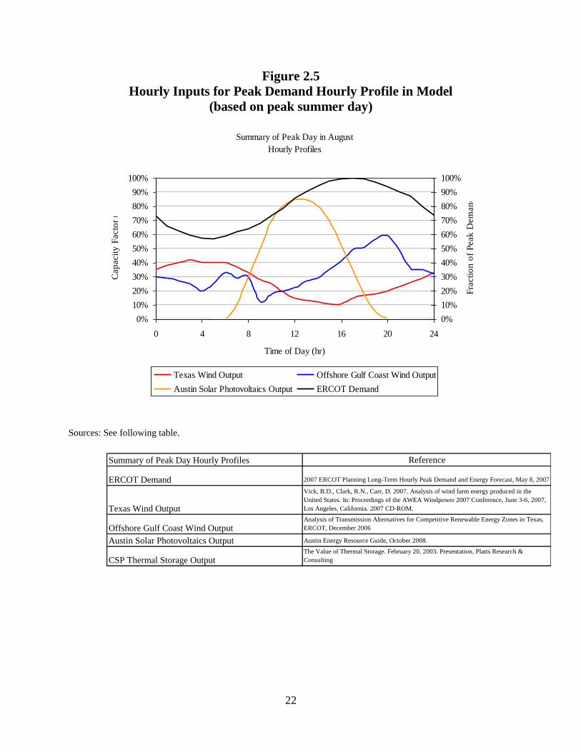
22

Figure 2.5

Hourly Inputs for Peak Demand Hourly Profile in Model

(based on peak summer day)

Sources: See following table.

Summary of Peak Day in August

Hourly Profiles

0%

10%

20%

30%

40%

50%

60%

70%

80%

90%

100%

0 4 8 12 16 20 24

Time of Day (hr)

Cap

acit

y F

acto

r (%

)

0%

10%

20%

30%

40%

50%

60%

70%

80%

90%

100%

Fra

cti

on

of

Peak

Dem

an

d (

%)

Texas Wind Output Offshore Gulf Coast Wind Output

Austin Solar Photovoltaics Output ERCOT Demand

Reference

2007 ERCOT Planning Long-Term Hourly Peak Demand and Energy Forecast, May 8, 2007

Vick, B.D., Clark, R.N., Carr, D. 2007. Analysis of wind farm energy produced in the

United States. In: Proceedings of the AWEA Windpower 2007 Conference, June 3-6, 2007,

Los Angeles, California. 2007 CD-ROM.

Analysis of Transmission Alternatives for Competitive Renewable Energy Zones in Texas,

ERCOT, December 2006

Austin Energy Resource Guide, October 2008.

The Value of Thermal Storage. February 20, 2003. Presentation, Platts Research &

ConsultingCSP Thermal Storage Output

Austin Solar Photovoltaics Output

Summary of Peak Day Hourly Profiles

ERCOT Demand

Texas Wind Output

Offshore Gulf Coast Wind Output

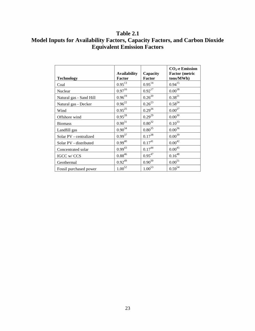
23

Table 2.1

Model Inputs for Availability Factors, Capacity Factors, and Carbon Dioxide

Equivalent Emission Factors

Technology

Availability

Factor

Capacity

Factor

CO2-e Emission

Factor (metric

tons/MWh)

Coal 0.9513

0.9514

0.9415

Nuclear 0.9716

0.9217

0.0018

Natural gas - Sand Hill 0.9619

0.2620

0.3821

Natural gas - Decker 0.9622

0.2623

0.5824

Wind 0.9525

0.2926

0.0027

Offshore wind 0.9528

0.2929

0.0030

Biomass 0.9031

0.8032

0.1033

Landfill gas 0.9034

0.8035

0.0036

Solar PV - centralized 0.9937

0.1738

0.0039

Solar PV - distributed 0.9940

0.1741

0.0042

Concentrated solar 0.9943

0.1744

0.0045

IGCC w/ CCS 0.8846

0.9547

0.1648

Geothermal 0.9249

0.9050

0.0051

Fossil purchased power 1.0052

1.0053

0.5954

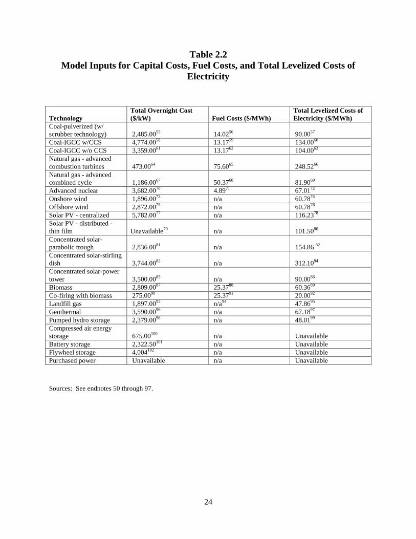
24

Table 2.2

Model Inputs for Capital Costs, Fuel Costs, and Total Levelized Costs of

Electricity

Technology

Total Overnight Cost

($/kW) Fuel Costs ($/MWh)

Total Levelized Costs of

Electricity ($/MWh)

Coal-pulverized (w/

scrubber technology) 2,485.0055

14.0256

90.0057

Coal-IGCC w/CCS 4,774.0058

13.1759

134.0060

Coal-IGCC w/o CCS 3,359.0061

13.1762

104.0063

Natural gas - advanced

combustion turbines 473.0064

75.6065

248.5266

Natural gas - advanced

combined cycle 1,186.0067

50.3768

81.9069

Advanced nuclear 3,682.0070

4.8971

67.0172

Onshore wind 1,896.0073

n/a 60.7874

Offshore wind 2,872.0075

n/a 60.7876

Solar PV - centralized 5,782.0077

n/a 116.2378

Solar PV - distributed -

thin film Unavailable79

n/a 101.5080

Concentrated solar-

parabolic trough 2,836.0081

n/a 154.86 82

Concentrated solar-stirling

dish 3,744.0083

n/a 312.1084

Concentrated solar-power

tower 3,500.0085

n/a 90.0086

Biomass 2,809.0087

25.3788

60.3689

Co-firing with biomass 275.0090

25.3791

20.0092

Landfill gas 1,897.0093

n/a94

47.8695

Geothermal 3,590.0096

n/a 67.1897

Pumped hydro storage 2,379.0098

n/a 48.0199

Compressed air energy

storage 675.00100

n/a Unavailable

Battery storage 2,322.50101

n/a Unavailable

Flywheel storage 4,004102

n/a Unavailable

Purchased power Unavailable n/a Unavailable

Sources: See endnotes 50 through 97.

25

Table 2.3

Primary Scenarios Run for Analysis

Scenario Title

Resources/Technologies

with Sensitivity

Analysis

Major Additions and

Subtractions Through

2020

Portfolio 1 AE Resource Plan

None Add biomass, natural gas,

solar, and wind

Portfolio 2 Nuclear Expansion Nuclear and natural gas Nuclear replaces coal and

AE resource plan

additions

Portfolio 3 High Renewables Onshore and offshore wind,

concentrated solar power,

centralized and distributed

PV, biomass, and

geothermal

Very high investments in

biomass, geothermal,

solar, and wind

technologies to replace

coal

Portfolio 4 Expected Renewables Refer to portfolio 3

sensitivity analysis

Expected available

investments in biomass,

geothermal, solar, and

onshore wind to replace

coal

Portfolio 5 Renewables with

Storage

Various energy storage

technologies

Expected renewables

coupled with energy

storage of wind to replace

coal

Portfolio 6 Natural Gas Expansion Natural gas, co-firing

biomass

Natural gas replaces half

of current coal and AE

resource plan additions

Portfolio 7 Cleaner Coal IGCC without carbon

capture and storage

technology

IGCC with carbon capture

and storage to replace

Fayette Power Project and

AE resource plan

additions

Portfolio 8 High Renewables

without Nuclear

Pulverized coal, IGCC with

and without carbon capture,

and natural gas

High renewables to

replace coal and nuclear

26

Notes

1 Hobbs, Benjamin F. “Optimization methods for electric utility resource planning.” European Journal of

Operational Research, vol. 83, no. 1, (May 18, 1995), pp. 1-20.

2 National Regulatory Research Institute. What Generation Mix Suits Your State? Tools for Comparing Fourteen

Technologies across Nine Criteria. Columbus, OH, February 14, 2007.

3 Govtrack.us, “S. 280: Climate Stewardship and Innovation Act of 2007. Online. Available:

http://www.govtrack.us/congress/bill.xpd?bill=s110-280. Accessed: January 20, 2009.

4 U.S. Environmental Protection Agency. “EPA Analysis of the Lieberman-Warner Climate Security Act of 2008, S.

2191 in 110th Congress.” March 14, 2008. Online. Available:

http://www.epa.gov/climatechange/economics/economicanalyses.html#s2191. Accessed : March 14, 2008.

5 Stan Kaplan. Congressional Research Service, Power Plants: Characteristics and Costs. November 13, 2008.

Online. Available: http://www.fas.org/sgp/crs/misc/RL34746.pdf. Accessed: December 15, 2008.

6 California Energy Commission, Comparative Costs of California Central Station Electricity Generation

Technologies(June 2007). Online. Available: http://www.energy.ca.gov/2007publications/CEC-200-2007-011/CEC-

200-2007-011-SD.PDF. Accessed: November 15, 2008. pp. 4-6.

7 “IMPLAN Professional 2.0: User’s Guide, Analysis Guide, Data Guide.” MIG, Inc., 2004. p. 102

8 “IMPLAN Professional 2.0: User’s Guide, Analysis Guide, Data Guide.” MIG, Inc., 2004. p. 103

9 US Department of Energy, Energy Efficiency and Renewable Energy, “Wind Powering America: Job and

Development Impact (JEDI) Model.” Available Online:

http://www.windpoweringamerica.gov/filter_detail.asp?itemid=707. Accessed: November 11 2008.

10 “IMPLAN Professional 2.0: User’s Guide, Analysis Guide, Data Guide.” MIG, Inc., 2004. p. 125-126

11 AE, “Future Energy Resources and CO2 Cap and Reduction Planning.” July 2008. Online. Available:

http://www.austinenergy.com/About%20Us/Newsroom/Reports/Future%20Energy%20Resources_%20July%2023.p

df. Accessed: July 24, 2008.

12 AE, “Nacogdoches Biomass Project Town Hall Meeting.” August 13, 2008. Online. Available:

http://www.austinenergy.com/biomassTownHallAugust2008.pdf. Accessed: August 17, 2008.

13 Calculations from AE documents, in accordance with National Regulatory Research Institute. What Generation

Mix Suits Your State? Tools for Comparing Fourteen Technologies across Nine Criteria. Columbus, OH, February

14, 2007.

27

14

Calculations from AE documents, in accordance with National Regulatory Research Institute. What Generation


14, 2007.

15 Calculations from AE's CCAR Emissions Computations Spreadsheet, 2007.



14, 2007.



14, 2007.





14, 2007.

20 Calculations from AE Documents, including CCAR Emissions Computations Spreadsheet, 2007.




14, 2007.

23 Calculations from AE Documents, including CCAR Emissions Computations Spreadsheet, 2007.






14, 2007.



28 Not applicable, assumed to be similar to onshore wind.

29 Not applicable, assumed to be similar to onshore wind.

28

30

National Regulatory Research Institute. What Generation Mix Suits Your State? Tools for Comparing Fourteen








34 Not applicable, assumed to be similar to biomass.

35 Not applicable, assumed to be similar to biomass.





38 The Value of Distributed Photovoltaics to AE and the City of Austin, Clean Power Research LLC, March 17,

2006, in accordance with National Regulatory Research Institute. What Generation Mix Suits Your State? Tools for

Comparing Fourteen Technologies across Nine Criteria. Columbus, OH, February 14, 2007.





41 The Value of Distributed Photovoltaics to AE and the City of Austin, Clean Power Research LLC, March 17,

2006, in accordance with National Regulatory Research Institute. What Generation Mix Suits Your State? Tools for

Comparing Fourteen Technologies across Nine Criteria. Columbus, OH, February 14, 2007.



43 Not applicable, assumed to be similar to solar PV.

44 Not applicable, assumed to be similar to solar PV.



29

46

National Regulatory Research Institute. What Generation Mix Suits Your State? Tools for Comparing Fourteen


47 Not applicable, assumed to be equal to capacity factor for traditional coal.









52 Not applicable, assumed to always be available for purchase.

53 Not applicable, assumed to always be available for purchase.



Online. Available: http://www.fas.org/sgp/crs/misc/RL34746.pdf. Accessed: December 15, 2008. High estimates

assumed 20% higher and low estimates assumed 10% lower due to mature technology status.

56 The National Regulatory Research Institute, What Generation Mix Suits Your State? Tools for Comparing

Fourteen Technologies Across Nine Criteria. Online. Available:

http://www.coalcandothat.com/pdf/35%20GenMixStateToolsAndCriteria.pdf. Accessed: July 16, 2008. p. 18-19.

High and low estimates assumed 5% higher and lower due to low volatility of coal prices.

57 High and Low estimates are from: Lazard, "Levilized Cost of Energy Analysis-Version 2.0 (June 2008). Online.

Available:

http://www.narucmeetings.org/Presentations/2008%20EMP%20Levelized%20Cost%20of%20Energy%20-

%20Master%20June%202008%20(2).pdf. Accessed: November 15, 2008. p. 10. Expected value estimated at lower

end of the range due to estimated cost of IGCC plant.



assumed 30% higher and low estimates assumed 10% lower due to immaturity of technology.





30

60

Expected value estimate from: Lazard, "Levilized Cost of Energy Analysis-Version 2.0 (June 2008). Online.

Available:


%20Master%20June%202008%20(2).pdf. Accessed: November 15, 2008. p. 10. High estimate assumed 30%

higher than expected value and low estimate assumed 10% lower than expected value due to immaturity of

technology.



assumed 30% higher and low estimates assumed 10% lower due to immaturity of technology.





63 Expected value estimate is from: Lazard, "Levilized Cost of Energy Analysis-Version 2.0 (June 2008). Online.

Available:


%20Master%20June%202008%20(2).pdf. Accessed: November 15, 2008. p. 9. Low estimate is from: California

Energy Commission, Comparative Costs of California Central Station Electricity Generation Technologies(June

2007). Online. Available: http://www.energy.ca.gov/2007publications/CEC-200-2007-011/CEC-200-2007-011-

SD.PDF. Accessed: November 15, 2008. p. 7. High estimate assumed 30% higher than expected value due to

immaturity of technology.

64 Energy Information Administration, Assumptions to the Annual Energy Outlook 2008 (June 2008). Online.

Available: http://www.eia.doe.gov/oiaf/aeo/assumption/pdf/electricity.pdf. p. 79. High estimates assumed 20%

higher and low estimates assumed 10% lower due to mature technology status.




High estimates assumed 50% higher and low estimates assumed 20% lower due to high volatility of natural gas

prices.

66 Expected value estimate is from: California Energy Commission, Comparative Costs of California Central

Station Electricity Generation Technologies(June 2007). Online. Available:

http://www.energy.ca.gov/2007publications/CEC-200-2007-011/CEC-200-2007-011-SD.PDF. Accessed: November

15, 2008. p. 7. High and low estimates are from: Lazard, "Levilized Cost of Energy Analysis-Version 2.0 (June

2008). Online. Available:


%20Master%20June%202008%20(2).pdf. Accessed: November 15, 2008. p. 9.




31

68

The National Regulatory Research Institute, What Generation Mix Suits Your State? Tools for Comparing



High estimates assumed 50% higher and low estimates assumed 20% lower due to high volatility of natural gas

prices.








70 For expected value: Stan Kaplan. Congressional Research Service, Power Plants: Characteristics and Costs.

November 13, 2008. Online. Available: http://www.fas.org/sgp/crs/misc/RL34746.pdf. Accessed: December 15,

2008. Low estimates: Assumed 10 percent lower than expected value from: Energy Information Administration,

Assumptions to the Annual Energy Outlook 2008 (June 2008). Online. Available:

http://www.eia.doe.gov/oiaf/aeo/assumption/pdf/electricity.pdf. p. 79. High estimates: David Schlissel and Bruce

Biewald. Synapse Energy Economics, Inc. Nuclear Power Plant Construction Costs. July 2008. Online. Available:

http://www.synapse-energy.com/Downloads/SynapsePaper.2008-07.0.Nuclear-Plant-Construction-Costs.A0022.pdf.

Accessed: December 15, 2008. Rounded from highest estimate of $8,000/kw.




High and low estimates assumed 5% higher and lower due to low volatility of uranium prices.




15, 2008. p. 7. High estimate from: Lazard, "Levilized Cost of Energy Analysis-Version 2.0 (June 2008). Online.

Available:


%20Master%20June%202008%20(2).pdf. Accessed: November 15, 2008. p. 9. Low estimate assumed 10% lower

than expected value.









32





assumed 20% higher and low estimates assumed 30% lower due to immature technology status.

76 Assumed the same as onshore wind due to lack of information. Expected value estimate is from: California

Energy Commission, Comparative Costs of California Central Station Electricity Generation Technologies(June

2007). Online. Available: http://www.energy.ca.gov/2007publications/CEC-200-2007-011/CEC-200-2007-011-

SD.PDF. Accessed: November 15, 2008. p. 7. High and low estimates are from: Lazard, "Levilized Cost of Energy

Analysis-Version 2.0 (June 2008). Online. Available:






78 Expected value estimate is from: California Energy Commission, Comparative Costs of California Central Station

Electricity Generation Technologies(June 2007). Online. Available:


15, 2008. p. 7. High estimates assumed 20% higher and low estimates assumed 20% lower due to mature

technology status.

79 Information not available.

80 High and Low estimates are from: Lazard, "Levilized Cost of Energy Analysis-Version 2.0 (June 2008). Online.

Available:


%20Master%20June%202008%20(2).pdf. Accessed: November 15, 2008. p. 10. Expected value estimate is average

of high and low estimate.







15, 2008. p. 7. Low estimate is from: Lazard, "Levilized Cost of Energy Analysis-Version 2.0 (June 2008). Online.

Available:


%20Master%20June%202008%20(2).pdf. Accessed: November 15, 2008. p. 10. High estimates assumed 20%

higher.

33

83

Based upon data for solar thermal. Energy Information Administration, Assumptions to the Annual Energy

Outlook 2008 (June 2008). Online. Available: http://www.eia.doe.gov/oiaf/aeo/assumption/pdf/electricity.pdf. p. 79.

High estimates assumed 20% higher and low estimates assumed 20% lower due to immature technology status.





technology status.

85 The National Renewable Energy Laboratory, Online. Power Technologies Energy Data Book, Online. Available:

http://www.nrel.gov/analysis/power_databook/docs/pdf/db_chapter02_csp.pdf. Accessed: October 28, 2008., pp.

18,20,22. High estimates assumed 20% higher and low estimates assumed 20% lower due to immature technology

status.

86 Expected value estimate is from: Lazard, "Levilized Cost of Energy Analysis-Version 2.0 (June 2008). Online.

Available:


%20Master%20June%202008%20(2).pdf. Accessed: November 15, 2008. p. 10. High estimates assumed 20%

higher and low estimates assumed 20% lower due to immature technology status.




88 This is an average of the range provided by: The National Regulatory Research Institute, What Generation Mix

Suits Your State? Tools for Comparing Fourteen Technologies Across Nine Criteria. Online. Available:


89 Expected value estimate is for wood waste from: California Energy Commission, Comparative Costs of

California Central Station Electricity Generation Technologies(June 2007). Online. Available:


15, 2008. p. 7. High and low estimates are unspecified biomass sources from: Lazard, "Levilized Cost of Energy

Analysis-Version 2.0 (June 2008). Online. Available:



90 High and low estimates are from: Lazard, "Levilized Cost of Energy Analysis-Version 2.0 (June 2008). Online.

Available:


%20Master%20June%202008%20(2).pdf. Accessed: November 15, 2008. p. 9. Expected value is the average of the

high and low estimates.

91 This is an average of the range provided by: The National Regulatory Research Institute, What Generation Mix

Suits Your State? Tools for Comparing Fourteen Technologies Across Nine Criteria. Online. Available:


34

92

High and low estimates are from: Lazard, "Levilized Cost of Energy Analysis-Version 2.0 (June 2008). Online.

Available:


%20Master%20June%202008%20(2).pdf. Accessed: November 15, 2008. p. 9. Expected value is the average of the

high and low estimates.




94 Assume fuel is tapped into at facility so no costs are incurred.




15, 2008. p. 7. High estimate is from from: Lazard, "Levilized Cost of Energy Analysis-Version 2.0 (June 2008).

Online. Available:


%20Master%20June%202008%20(2).pdf. Accessed: November 15, 2008. p. 9. Low estimate assumed 10% lower





97 Expected value estimate is for binary plant from: California Energy Commission, Comparative Costs of

California Central Station Electricity Generation Technologies(June 2007). Online. Available:


15, 2008. p. 7. Low estimate is from from: Lazard, "Levilized Cost of Energy Analysis-Version 2.0 (June 2008).

Online. Available:


%20Master%20June%202008%20(2).pdf. Accessed: November 15, 2008. p. 9. High estimate assumed 20% higher


98 Expected value estimate is from: The National Regulatory Research Institute, What Generation Mix Suits Your

State? Tools for Comparing Fourteen Technologies Across Nine Criteria. Online. Available:


High and low estimates from: Dan Rastler, New Demand for Energy Storage, Electric Perspectives.

(September/October 2008) p. 30-47. Online. Available:

http://www.eei.org/magazine/editorial_content/nonav_stories/2008-09-01-EnergyStorage.pdf. Accessed: November

17, 2008.

99 Assumed expected value estimate for conventional hydropower from: California Energy Commission,

Comparative Costs of California Central Station Electricity Generation Technologies(June 2007). Online. Available:


35


technology status.

100 For below ground took average of high and low estimate from: Dan Rastler, New Demand for Energy Storage,

Electric Perspectives. (September/October 2008) p. 30-47. Online. Available:


17, 2008.

101 Took average of low and high estimates for lead acid, sodium, and flow batteries from: Dan Rastler, New

Demand for Energy Storage, Electric Perspectives. (September/October 2008) p. 30-47. Online. Available:


17, 2008.

102 Took average of low and high estimates for lead acid, sodium, and flow batteries from: Dan Rastler, New

Demand for Energy Storage, Electric Perspectives. (September/October 2008) p. 30-47. Online. Available:


17, 2008.

36

Chapter 3. Baseline Scenario: Austin Energy’s Proposed

Resource Plan

In July 2008 Austin Energy (AE) revealed a proposed resource plan for meeting energy

demand through 2020 while remaining under a proposed carbon dioxide (CO2) cap and

reduction plan.1 AE proposed adding 1,375 additional Megawatts (MW) of generating

capacity by 2020, with only 300 MW coming from fossil-fueled resources.2 Table 3.1

lists the planned additions to AE’s resource portfolio from 2009 to 2020 by fuel source,

power generation technology, or facility. The generation capacity for 2008 includes AE’s

current power generation mix. Scheduled additions of natural gas and wind power

generation capacity in 2009, 100 MW biomass project expected by 2012, and a 30 MW

centralized photovoltaic power plant located in Webberville just outside of Austin have

already been approved by the Austin City Council (Council) and contracted for purchase

or operation by AE. As a resource, biomass has a capacity factor similar to that of coal

and nuclear and can provide a reliable source of baseload power.3 This generating

capacity has been contracted through a PPA to provide 100 MW of energy per year over

a 20 year time period at the total cost of $2.3 billion. The wind and natural gas planned

additions for 2009, planned wind additions for 2011, the centralized photovoltaic (PV)

module system expected to be available by 2010, and the biomass project expected to be

available by 2012 have been included in all eight scenario runs. Cost projections for these

additions are based upon general cost data for new power generation plants, rather than

the contractual agreements established by AE.

AE’s proposed energy resource plan includes 200 MW of additional capacity at the Sand

Hill Energy Center, proposed for 2013. This would be a combined cycle expansion

project that would provide reliable energy with lower MW-hour (MWh) CO2 emissions

than coal. AE is expecting this project to cost $160 million and take three years to

complete.4 An additional 100 MW of purchased biomass generating capacity has also

been recommended for 2016. AE’s primary investment in new generation capacity is an

addition of 775 MW of generating capacity from wind facilities. Additionally, contracts

for 77 MW and 126 MW of current wind generating capacity being purchased by AE are

set to expire in 2011 and 2017, respectively. AE may be able to renew these contracts at

that time. AE has also proposed a gradual investment in solar energy to meet the Austin

Climate Protection Plan (ACPP) goal of providing 100 MW of solar capacity by 2020.

The recently approved 30 MW centralized PV solar facility will be constructed in

Webberville, near Manor, Texas. This facility will also have 5 MW of capacity to test

emerging solar technologies. AE is planning to invest in covering rooftop space in Austin

with photovoltaic modules (PV) through public and private partnerships to help reach its

solar goals. AE also may invest in a large-scale West Texas solar plant.5 It is unclear

whether the solar capacity additions for the years 2014, 2017, and 2019 are expected to

come from distributed solar PVs, centralized PV power plants, or concentrated solar

power plants. For the purposes of this analysis, it has been assumed that the 2014 and

2017 additions will be investments in distributed PV systems and the 2019 addition will

be a concentrating solar power plant.

37

System Reliability

AE’s proposed resource plan provides a baseline proposal for adequately meeting

expected increased demand through 2020 while satisfying AE’s proposed CO2 emissions

cap and reduction plan, as well as specific goals detailed by the ACPP. demonstrates that

AE’s power generation capacity will well exceed forecasted peak load with and without

meeting conservation goals. By 2016, 1,229 MW of power generation capacity will be

provided from baseload power sources (coal, nuclear, and biomass). The 100 MW

biomass additions set to occur in 2012 and 2016 continue to help AE provide continuous

power from traditional baseload power sources in accordance with expected baseload

demand increases. Solar and wind capacity increases should provide increased renewable

energy for AE customers that can be backed-up by the natural gas plants. The 300 MW of

additional natural gas power generation capacity lends towards this system of dependable

power that will help account for any unexpected lags in availability due to the

intermittent nature of wind and solar resources.

Given the expected capacity factors for on-shore wind and solar PV (29 and 17 percent,

respectively) as well as current capacity factors for AE’s coal, nuclear, and natural gas

facilities AE will be able to deliver electricity reliably to its customers, given that AE

meets its conservation goals (see Figure 3.2). It appears that AE will be able to provide

reliable service even if conservation goals are only met halfway.

Figure 3.3 details AE’s expected hourly load profile for the hottest day (peak demand) in

the summer of 2020. The hourly load profile follows expected solar and wind profiles

and demonstrates that AE will be able to meet peak demand without purchasing power by

engaging its natural gas facilities, even on the hottest day of the summer. As AE makes

gradual additions to its resource portfolio from baseload, intermediate, and intermittent

sources of energy, it appears that AE will be able to meet peak demand in all years

between 2009 and 2020 without purchasing power. AE is currently purchasing 300 MW

of power a year from the statewide electric grid. AE’s planned resource portfolio allows

AE to control all of its power generation resources.

Carbon Emissions and Carbon Costs

AE’s proposed resource plan will increase the amount of renewable power generation

capacity to about 30 percent of its resource portfolio by 2020. About 27 percent of AE’s

actual power generation would come from clean energy sources in 2020. As peak demand

is expected to increase by about 16 percent between 2008 and 2020, the increase in clean

energy power generation capacity (by about 22 percent) will not curb CO2 emissions

markedly (see Figure 3.4). The resource portfolio shift to a higher percentage of clean

energy sources allows AE to meet increased demand without a concurrent rise in CO2

emissions.

In July 2008 AE proposed a CO2 upper limit (cap) and reduction plan through 2020.6 AE

plans to cap its CO2 emissions at 2007 emission levels and gradually reduce emissions to

2005 levels by 2014. Most recently proposed federal carbon-related bills would set an

38

initial 2014 goal of reducing economy-wide greenhouse gas (GHG) emissions to 2005 or

2006 levels in the first year of implementation. AE’s CO2 emissions in 2007 were

roughly 6.1 million metric tons and in 2005 were roughly 5.6 million metric tons. AE will

need to reduce its emissions by 745,000 million metric tons over a seven-year period

while energy demands gradually rise. Their goal is to gradually reduce emissions by

about 100,000 metric tons in a stair-step fashion.

While no current carbon regulation exists, many bills have been proposed by the United

States Congress over the past several years. Many of these bills propose a cap-and-trade

system that would give away CO2 allowances to regulated entities to ease the burden of

the regulations. However, these allowances are typically based upon recent historical

emissions, so a voluntary program for curbing CO2 emissions could reduce the number of

allowances AE might receive in the future.7 Under the Lieberman-Warner Climate

Security and Stewardship Act of 2007, a portion of an entity’s emissions would be

accounted for by free permits, or allowances, while a portion of allowances would be

auctioned.8 Figure 3.5 estimates the costs of allowances for AE based upon the

Lieberman-Warner bill and expected CO2 emissions under AE’s proposed resource plan.

Since the amount of permits would gradually decline under the proposed cap and trade

system, the cost of allowances would rise from almost $50 million in 2014 to almost

$100 million in 2020, for a total of about $490 million in carbon allowance costs by

2020. Although the expected cost of offsets is expected to be lower than the cost of

allowances, only 15 percent of an entity’s CO2 emissions could be accounted for as

offsets under the Lieberman-Warner bill.9

AE has stated that given current economic and political considerations, the best option for

reducing its carbon footprint is to generate electricity from its current sources and

purchase offsets in the short-term for emissions that exceed the cap and/or replace coal-

based generation with natural gas.10

If the federal government or the State of Texas were

to adopt comprehensive GHG regulations, AE will be able to make a more informed

decision on these options. AE projects that costs to offset CO2 emissions by 2014 would

be $18.8 million dollars, while replacing coal generation with natural gas would cost

$253.3 million.11

Figure 3.6 provides a range of annual costs to offset emissions to zero,

thus achieving carbon-neutrality. Depending on the cost of offsets, offsetting emissions to

zero would range between $50 million and $250 million annually with a slight decline in

costs most years.

AE’s proposed resource plan presents marked improvement in delivering electricity from

clean and renewable sources, which tend to have less impact on air and water quality,

land, and local ecosystems. However, AE’s resource plan does not plan on selling or

reducing its stake in its coal or nuclear resources, so the environmental impacts

associated with these resources will continue to persist. AE’s coal resources currently

account for 71 percent of its total CO2 emissions. Continued use of coal prevents

significant reductions in CO2 emissions. Other harmful air and water pollutants generated

by its coal facility will continue to impact the environment negatively. Nuclear waste will

also continue to accumulate due to AE’s nuclear resource use. Despite the remaining

sustainability issues associated with AE’s coal and nuclear resources, it appears that AE’s

39

proposed energy resource plan moves towards a more sustainable energy portfolio,

particularly to account for increased energy demand.


The approach of the report is to project costs and economic impacts based solely upon

general cost estimates for new power generation facilities. The model used here does not

reflect AE’s cost projections of scheduled or proposed additions to its resource portfolio,

whether in the form of power purchase agreements or currently owned and operated

facility expansions, the following cost estimates may not coincide with AE projections.

Figure 3.7 lists capital cost estimates for AE’s scheduled and proposed additions to its

power generation mix. Capital costs are expressed as the sum of total overnight costs for

additions scheduled in a particular year. Total expected capital costs summed over the

years until 2020 range from $2.2 to $3.0 billion. The year in which a project is proposed

influences total capital costs. This study uses a range of costs, even though expected

capital costs may increase or decrease during the next decade. AE’s proposed energy

resource plan demonstrates gradual capital investments to account for increased demand.

AE has no plans to sell current power generation facilities or stakes in current facilities.

The majority of AE’s planned projects do not have large capital cost ranges.

Figure 3.8 details annual expected fuel costs for AE’s proposed resource plan. As fossil-

fueled sources do not change dramatically under this scenario, fuel costs are expected to

remain fairly stable, ranging in any given year from $170 to $360 million. If carbon

legislation or other fossil-fueled related regulation is implemented over the next decade,

fuel costs (primarily for coal and natural gas) should move towards the high range.

Figure 3.9 estimates the expected rise in costs to produce electricity by calculating the

impact of the levelized costs of new power generation resources, as a percentage of

overall generation capacity. As a resource portfolio becomes composed of more new

resource additions, the marginal increase in costs will rise. AE’s energy resource plan

calls for almost 30 percent of its 2020 resource portfolio to be comprised of new

generation capacity, which leads to an increase of between 1.5 and 3 cents per kilowatt-

hour between 2009 and 2020 based on new power generation investments alone. Carbon

allowance costs and offset costs or any unexpected additional costs to the utility could

also be passed on to the customer during this time period.

The Greater Austin Area is expected to experience significant economic stimulation from

the AE resource plan due to expansion of local natural gas facilities and investment in

local solar PV installation and utility-scale solar PV power plants. Figure 3.10

demonstrates an average of $90 million in additional total economic output through 2020.

Economic activity will peak at approximately $180 million in 2011 and 2012 in

anticipation of the completion of a 200 MW expansion to the Sand Hill natural gas

facility in 2013 and solar capacity additions expected in 2014. Total economic output will

rise again in 2016 to almost $130 million due to additional solar capacity additions.

Figure 3.11 projects $3.6 million of total value added due to enduring economic activity.

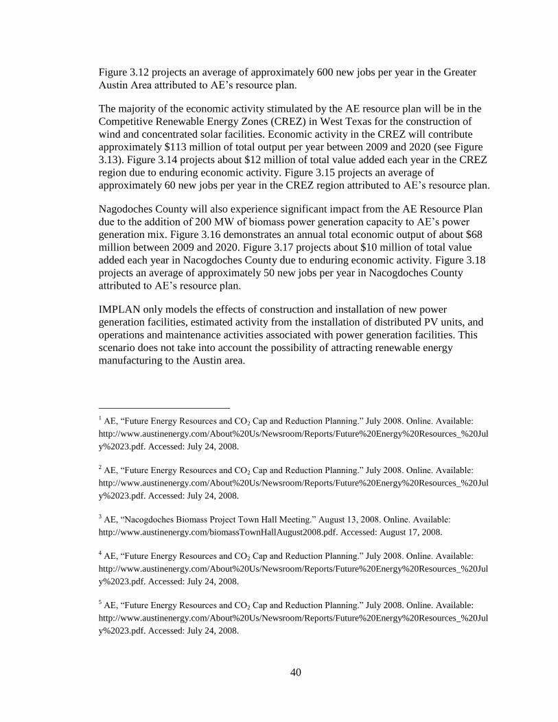
40

Figure 3.12 projects an average of approximately 600 new jobs per year in the Greater

Austin Area attributed to AE’s resource plan.

The majority of the economic activity stimulated by the AE resource plan will be in the

Competitive Renewable Energy Zones (CREZ) in West Texas for the construction of

wind and concentrated solar facilities. Economic activity in the CREZ will contribute

approximately $113 million of total output per year between 2009 and 2020 (see Figure

3.13). Figure 3.14 projects about $12 million of total value added each year in the CREZ

region due to enduring economic activity. Figure 3.15 projects an average of

approximately 60 new jobs per year in the CREZ region attributed to AE’s resource plan.

Nagodoches County will also experience significant impact from the AE Resource Plan

due to the addition of 200 MW of biomass power generation capacity to AE’s power

generation mix. Figure 3.16 demonstrates an annual total economic output of about $68

million between 2009 and 2020. Figure 3.17 projects about $10 million of total value

added each year in Nacogdoches County due to enduring economic activity. Figure 3.18

projects an average of approximately 50 new jobs per year in Nacogdoches County

attributed to AE’s resource plan.

IMPLAN only models the effects of construction and installation of new power

generation facilities, estimated activity from the installation of distributed PV units, and

operations and maintenance activities associated with power generation facilities. This

scenario does not take into account the possibility of attracting renewable energy

manufacturing to the Austin area.







3 AE, “Nacogdoches Biomass Project Town Hall Meeting.” August 13, 2008. Online. Available:

http://www.austinenergy.com/biomassTownHallAugust2008.pdf. Accessed: August 17, 2008.








Available:



7 Austin Energy, “Austin Smart Energy.” Austin Energy Resource Guide. Online. Available:

http://www.austinsmartenergy.com/downloads/AustinEnergyResourceGuide.pdf. Accessed: December 19,

2008, p 35.

8 Govtrack.us. “S. 2191 [110

th] Lieberman-Warner Climate Security Act of 2007.” Online. Available:


9 Govtrack.us. “S. 2191 [110

th] Lieberman-Warner Climate Security Act of 2007.” Online. Available:



Available:




Available:



42

Table 3.1

Austin Energy Resource Plan Scheduled Additions to Generation Mix

2008 2009 2010 2011 2012 2013 2014 2015 2016 2017 2018 2019 2020

Coal 607 0 0 0 0 0 0 0 0 0 0 0 0

Nuclear 422 0 0 0 0 0 0 0 0 0 0 0 0

Natural Gas - Sand Hill 1-4 189 100 0 0 0 0 0 0 0 0 0 0 0

Natural Gas - Sand Hill 5 312 0 0 0 0 200 0 0 0 0 0 0 0

Natural Gas - Decker 1 & 2 741 0 0 0 0 0 0 0 0 0 0 0 0

Natural Gas - Decker CGT 193 0 0 0 0 0 0 0 0 0 0 0 0

Wind 274 165 0 23 0 0 50 100 0 74 0 50 110

Offshore Wind 0 0 0 0 0 0 0 0 0 0 0 0 0

Biomass 0 0 0 0 100 0 0 0 100 0 0 0 0

FPP w/ biomass co-firing 0 0 0 0 0 0 0 0 0 0 0 0 0

Landfill Gas 12 0 0 0 0 0 0 0 0 0 0 0 0

Solar PV - Centralized 0 0 30 0 0 0 0 0 0 0 0 0 0

Solar PV - Distributed 1 0 0 0 0 0 20 0 0 20 0 0 0

Concentrated Solar 0 0 0 0 0 0 0 0 0 0 0 30 0

IGCC w/ CCS 0 0 0 0 0 0 0 0 0 0 0 0 0

IGCC w/o CCS 0 0 0 0 0 0 0 0 0 0 0 0 0

Geothermal 0 0 0 0 0 0 0 0 0 0 0 0 0

Storage 0 0 0 0 0 0 0 0 0 0 0 0 0

Accelerated Conservation 0 0 0 0 0 0 0 0 0 0 0 0 0

Purchased Power 0 0 0 0 0 0 0 0 0 0 0 0 0

Schedule of power generation additions and subtractions (net MW)

43

Figure 3.1

Austin Energy Resource Plan Power Generation Capacity

Austin Energy Electric Generation Capacity (MW)

0

500

1,000

1,500

2,000

2,500

3,000

3,500

4,000

2008 2009 2010 2011 2012 2013 2014 2015 2016 2017 2018 2019 2020

Concentrated Solar

Solar PV - Distributed

Solar PV - Centralized

Wind

Natural Gas - Decker CGT

Natural Gas - Decker 1 & 2

Natural Gas - Sand Hill 5

Natural Gas - Sand Hill 1-4

Landfill Gas

Biomass

Nuclear

Coal

Peak load forecast w/ conservation

Peak load forecast w/o conservation

Cap

acity

(M

W)

44

Figure 3.2

Austin Energy Resource Plan Electric Delivery

Austin Energy Electric Delivery (MWh)

0

2,000,000

4,000,000

6,000,000

8,000,000

10,000,000

12,000,000

14,000,000

16,000,000

2008 2009 2010 2011 2012 2013 2014 2015 2016 2017 2018 2019 2020

Concentrated Solar



Wind





Landfill Gas

Biomass

Nuclear

Coal


Peak load forecast w/ no policy

En

erg

y D

eli

vere

d (

MW

h)

45

Figure 3.3

Austin Energy Resource Plan Hourly Load Profile (Peak Demand, Summer 2000)

Hourly load profile (MW)

Peak demand, summer of 2020

0

500

1,000

1,500

2,000

2,500

3,000

3,500

4,000

0 4 8 12 16 20 24

Hour of day

Coal Nuclear

Biomass Landfill Gas

Natural Gas - Sand Hill 1-4 Natural Gas - Sand Hill 5

Natural Gas - Decker 1 & 2 Natural Gas - Decker CGT

Wind Offshore Wind

Solar PV - Centralized Solar PV - Distributed

Concentrated Solar Peak load forecast w/o conservation


Pea

k D

eman

d (M

W)

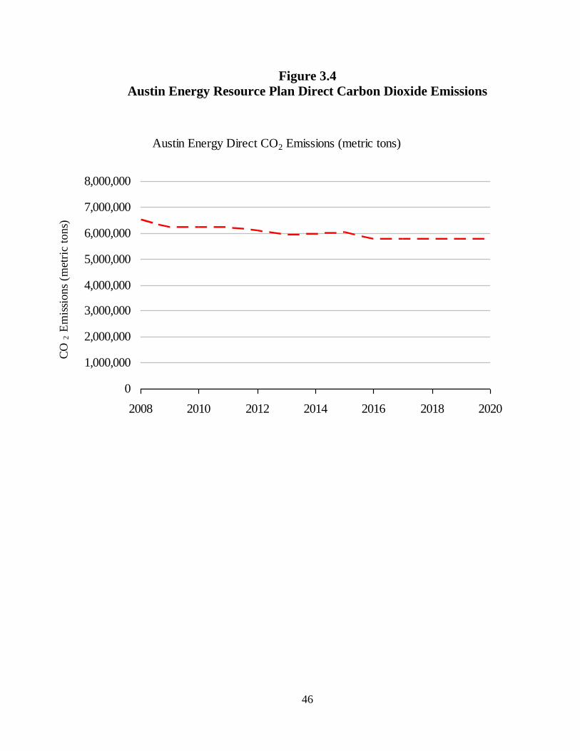
46

Figure 3.4

Austin Energy Resource Plan Direct Carbon Dioxide Emissions

Austin Energy Direct CO2 Emissions (metric tons)

0

1,000,000

2,000,000

3,000,000

4,000,000

5,000,000

6,000,000

7,000,000

8,000,000

2008 2010 2012 2014 2016 2018 2020

CO

2 E

mis

sio

ns

(met

ric

ton

s)

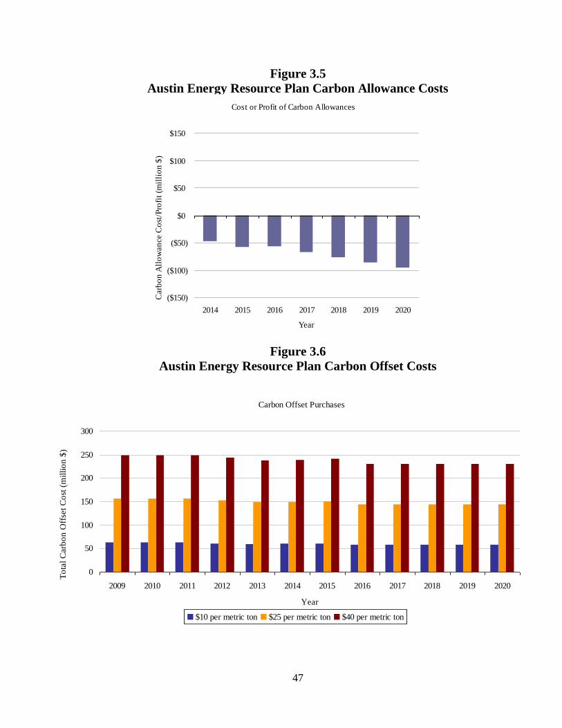
47

Figure 3.5

Austin Energy Resource Plan Carbon Allowance Costs

Figure 3.6

Austin Energy Resource Plan Carbon Offset Costs

Cost or Profit of Carbon Allowances

($150)

($100)

($50)

$0

$50

$100

$150

2014 2015 2016 2017 2018 2019 2020

Year

Carb

on

All

ow

an

ce C

ost

/Pro

fit

(mil

lio

n $

)

Carbon Offset Purchases

0

50

100

150

200

250

300

2009 2010 2011 2012 2013 2014 2015 2016 2017 2018 2019 2020

Year

$10 per metric ton $25 per metric ton $40 per metric ton

To

tal

Carb

on

Off

set

Co

st (

mil

lio

n $

)

48

Figure 3.7

Austin Energy Resource Plan Capital Costs

Figure 3.8

Austin Energy Resource Plan Fuel Costs

Expected Capital Cost

$0

$100

$200

$300

$400

$500

$600

$700

$800

$900

$1,000

2009 2010 2011 2012 2013 2014 2015 2016 2017 2018 2019 2020

Year

Cap

ital

Co

st (

mil

lio

n $

)

Expected Fuel Cost

$-

$100

$200

$300

$400

$500

$600

$700

$800

$900

$1,000

2009 2010 2011 2012 2013 2014 2015 2016 2017 2018 2019 2020

Year

Fuel

Cost

(m

illi

on $

)

49

Figure 3.9

Austin Energy Resource Plan Levelized Costs

Expected Levelized Cost Increase Due to Electric Generation Capacity Additions

0

1

2

3

4

5

6

7

8

9

10

2009 2010 2011 2012 2013 2014 2015 2016 2017 2018 2019 2020

0%

10%

20%

30%

40%

50%

60%

70%

80%

90%

100% Concentrated Solar



Wind





Landfill Gas

Biomass

Nuclear

Coal

Expected Increase in LCOE

Gen

era

tion

from

Cap

acity

Ad

ditio

ns (%

)

Ex

pecte

d I

ncre

ase

in

Lev

eli

zed

Ele

ctr

icit

y C

ost

(cen

ts/k

Wh

)

50

Figure 3.10

Austin Energy Resource Plan Economic Activity Greater Austin Area

Figure 3.11

Austin Energy Resource Plan Total Value Added Greater Austin Area

Figure 3.12

Austin Energy Resource Plan Employment Impacts Greater Austin

Area

$0

$20,000,000

$40,000,000

$60,000,000

$80,000,000

$100,000,000

$120,000,000

$140,000,000

$160,000,000

$180,000,000

$200,000,000

2006

2007

2008

2009

2010

2011

2012

2013

2014

2015

2016

2017

2018

2019

2020

Output (induced)

Output (indirect)

Output (direct)

$0

$10,000,000

$20,000,000

$30,000,000

$40,000,000

$50,000,000

$60,000,000

$70,000,000

$80,000,000

$90,000,000

$100,000,000

2006

2007

2008

2009

2010

2011

2012

2013

2014

2015

2016

2017

2018

2019

2020

Value added (induced)

Value added (indirect)

Value added (direct)

0

200

400

600

800

1,000

1,200

1,400

1,600

2006

2007

2008

2009

2010

2011

2012

2013

2014

2015

2016

2017

2018

2019

2020

Employment (induced)

Employment (indirect)

Employment (direct)

51

Figure 3.13

Austin Energy Resource Plan Economic Activity CREZ Region

Figure 3.14

Austin Energy Resource Plan Total Value Added CREZ Region

Figure 3.15

Austin Energy Resource Plan Employment Impacts CREZ Region

$0

$20,000,000

$40,000,000

$60,000,000

$80,000,000

$100,000,000

$120,000,000

$140,000,000

$160,000,000

$180,000,000

$200,000,000

20

07

20

08

20

09

20

10

20

11

20

12

20

13

20

14

20

15

20

16

20

17

20

18

20

19

20

20

Output (direct)

Output (indirect)

Output (induced)

Output (total)

$0

$20,000,000

$40,000,000

$60,000,000

$80,000,000

$100,000,000

$120,000,000

$140,000,000

$160,000,000

20

07

20

08

20

09

20

10

20

11

20

12

20

13

20

14

20

15

20

16

20

17

20

18

20

19

20

20

TVA (direct)

TVA (indirect)

TVA (induced)

TVA (total)

0.00

200.00

400.00

600.00

800.00

1,000.00

1,200.00

1,400.00

1,600.00

1,800.00

2007200

8200

9201

0201

1201

2201

3201

4201

5201

6201

7201

8201

9202

0

Employment (direct)



Employment (total)

52

Figure 3.16

Austin Energy Resource Plan Economic Activity Nacogdoches County

Figure 3.17

Austin Energy Resource Plan Total Value Added Nacogdoches County

Figure 3.18

Austin Energy Resource Plan Employment Impacts Nacogdoches

County

$0

$20,000,000

$40,000,000

$60,000,000

$80,000,000

$100,000,000

$120,000,000

$140,000,000

20

09

20

10

20

11

20

12

20

13

20

14

20

15

20

16

20

17

20

18

20

19

20

20

Output (direct)

Output (indirect)

Output (induced)

Output (total)

$0

$10,000,000

$20,000,000

$30,000,000

$40,000,000

$50,000,000

$60,000,000

$70,000,000

20

09

20

10

20

11

20

12

20

13

20

14

20

15

20

16

20

17

20

18

20

19

20

20

TVA (direct)

TVA (indirect)

TVA (induced)

TVA (total)

0.00

200.00

400.00

600.00

800.00

1,000.00

1,200.00

20

09

20

10

20

11

20

12

20

13

20

14

20

15

20

16

20

17

20

18

20

19

20

20

Employment (direct)



Employment (total)

53

Notes

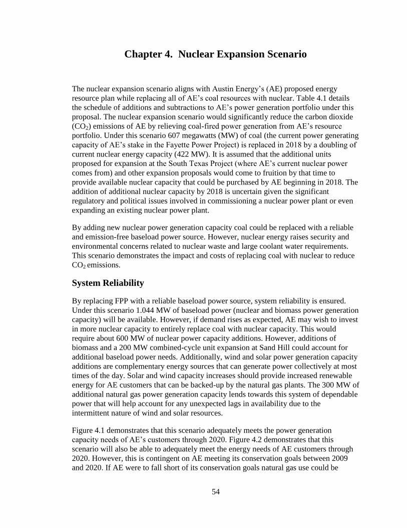
54

Chapter 4. Nuclear Expansion Scenario

The nuclear expansion scenario aligns with Austin Energy’s (AE) proposed energy

resource plan while replacing all of AE’s coal resources with nuclear. Table 4.1 details

the schedule of additions and subtractions to AE’s power generation portfolio under this

proposal. The nuclear expansion scenario would significantly reduce the carbon dioxide

(CO2) emissions of AE by relieving coal-fired power generation from AE’s resource

portfolio. Under this scenario 607 megawatts (MW) of coal (the current power generating

capacity of AE’s stake in the Fayette Power Project) is replaced in 2018 by a doubling of

current nuclear energy capacity (422 MW). It is assumed that the additional units

proposed for expansion at the South Texas Project (where AE’s current nuclear power

comes from) and other expansion proposals would come to fruition by that time to

provide available nuclear capacity that could be purchased by AE beginning in 2018. The

addition of additional nuclear capacity by 2018 is uncertain given the significant

regulatory and political issues involved in commissioning a nuclear power plant or even

expanding an existing nuclear power plant.

By adding new nuclear power generation capacity coal could be replaced with a reliable

and emission-free baseload power source. However, nuclear energy raises security and

environmental concerns related to nuclear waste and large coolant water requirements.

This scenario demonstrates the impact and costs of replacing coal with nuclear to reduce

CO2 emissions.

System Reliability

By replacing FPP with a reliable baseload power source, system reliability is ensured.

Under this scenario 1.044 MW of baseload power (nuclear and biomass power generation

capacity) will be available. However, if demand rises as expected, AE may wish to invest

in more nuclear capacity to entirely replace coal with nuclear capacity. This would

require about 600 MW of nuclear power capacity additions. However, additions of

biomass and a 200 MW combined-cycle unit expansion at Sand Hill could account for

additional baseload power needs. Additionally, wind and solar power generation capacity

additions are complementary energy sources that can generate power collectively at most

times of the day. Solar and wind capacity increases should provide increased renewable

energy for AE customers that can be backed-up by the natural gas plants. The 300 MW of

additional natural gas power generation capacity lends towards this system of dependable

power that will help account for any unexpected lags in availability due to the

intermittent nature of wind and solar resources.

Figure 4.1 demonstrates that this scenario adequately meets the power generation

capacity needs of AE’s customers through 2020. Figure 4.2 demonstrates that this

scenario will also be able to adequately meet the energy needs of AE customers through

2020. However, this is contingent on AE meeting its conservation goals between 2009

and 2020. If AE were to fall short of its conservation goals natural gas use could be

55

increased accordingly. Figure 4.3 details AE’s expected hourly load profile for the hottest

day (peak demand) in the summer of 2020. Under this scenario AE would fall just short

of meeting peak demand in 2020 (meeting 98.8 percent of energy needs at peak) without

purchasing power from the electric grid. This is considering that natural gas facilities are

run at full capacity during peak demand periods and follows expected wind and solar

availability profiles. This demonstrates that it may be necessary for AE to add additional

nuclear capacity or additional capacity from other energy sources to provide peak power

in 2020.


This scenario would cut carbon emissions by almost three quarters, primarily a result of

eliminating coal from AE’s resource portfolio. In 2007 AE emitted roughly 6.1 million

metric tons of CO2. Under the nuclear expansion scenario CO2 emissions would drop to

under 2 million metric tons by 2020 (see Figure 4.4). The nuclear expansion scenario

demonstrates an opportunity to significantly reduce AE’s carbon footprint to a level that

makes offsetting emissions to zero more manageable than under AE’s proposed resource

plan.

Significantly reducing CO2 emissions could present an opportunity to profit if carbon

regulation were to be passed that supported a portion of allowances being given for free.

Figure 4.5 indicates that AE will begin to accrue profits from carbon trading in 2018 with

the transition of coal to nuclear. By 2020 AE could be profiting roughly $55 million

annually from excess carbon allowances. Figure 4.6 shows the effects on the quantity of

carbon offsets required for purchase by AE annually to reach zero net carbon emissions.

In 2020 it would cost AE roughly $41 million annually at a offset cost of $25 per metric

ton of CO2 released to reach carbon neutrality through offsetting emissions.


The most significant cost incurred by AE under this scenario is the expansion of nuclear

capacity. Nuclear facilities have high capital costs with much uncertainty. Cost estimates

have escalated during the past several years as more realistic estimates for nuclear power

plant projects have been released. Nuclear plant capital cost estimates range from $3,000

to $8,000 per kilowatt installed. This would mean an overnight cost of between $1.3

billion and $3.4 billion for 422 MW of nuclear power generation capacity. However, fuel

costs and operating costs are lower than other energy resources given the levels of energy

output from these facilities. Figure 4.7 shows a distinctive spike in capital expenditures in

2018 attributed to nuclear power generation expansion. Figure 4.8 demonstrates that

under this scenario fuel costs would remain steady through 2020 because even when coal

is removed natural gas would be used more heavily to account for some loss in net

baseload power. It is important to recognize that although nuclear power plants require

significant initial capital investment, operations and maintenance costs are more

predictable and stable than other power generation technologies once the plant becomes

operational.

56

Figure 4.9 shows the expected increase in the cost of electricity in 2017 would be about 2

cents per kWh, but would then jump to about a 4 cent per kWh increase over current rates

in 2018 due to nuclear additions. If the cost of nuclear is higher than expected the cost of

electricity could increase as much as 6 cents per kWh over current rates. While AE may

not be directly involved in the funding of the construction of the facility from which this

nuclear power would be purchased, it is assumed that the costs of capital will be

accounted for in the levelized cost of electricity. This scenario and some other scenarios

include the divestment of all or a portion of AE’s stake in FPP. The calculation provided

by Figure 4.9 for expected increase in cost of electricity does not appoint a monetary

value of reducing or removing coal or any other resource from AE’s resource portfolio as

the methods for evaluating how much AE could receive are beyond the scope of this

report. Such removal may help to alleviate the additional costs to electricity accrued from

the identified resource additions. Additionally, the cost estimates provided in this model

do not account for any government subsidies that may be available for the building of

new nuclear power plants.

The biggest additions to AE’s resource portfolio that occur in the nuclear expansion

scenario are external to the Greater Austin Area. Wind and concentrated solar

investments are projected to be located in the Competitive Renewable Energy Zones

(CREZ) and nuclear capacity additions are projected to be located at in Matagorda Bay at

the South Texas Project based upon proposals to expand this facility. Investment in local

power generation will not likely offset the negative local economic impacts of divestment

in AE’s coal use. Figure 4.10 shows the economic output in the Greater Austin Area

generated by the nuclear expansion scenario and Figure 4.11 shows the total value added

to the Greater Austin Area from the investments made in the nuclear expansion scenario.

The simulation projects that the average local economic development attributed to the

nuclear expansion scenario prior to divestment in coal will be $125 million in economic

output and 824 additional jobs per year. $150 million would be generated in both 2011

and 2012, mostly due to the 200 MW expansion project of 200 MW of new natural gas-

based power generation capacity at Sand Hill in 2013. Economic output increases to over

$200 million in 2014 and 2017 corresponding to the addition of 20 MW of distributed

solar PV capacity in each year. Figure 4.12 shows the impacts on employment created or

eliminated by the nuclear expansion scenario. Divestment in AE’s stake in FPP in 2018 is

expected to create a net loss of 36 jobs in the Greater Austin Area.

57

Table 4.1

Nuclear Expansion Scenario Scheduled Additions and Subtractions to Generation Mix

2008 2009 2010 2011 2012 2013 2014 2015 2016 2017 2018 2019 2020

Coal 607 0 0 0 0 0 0 0 0 0 -607 0 0

Nuclear 422 0 0 0 0 0 0 0 0 0 422 0 0





Wind 274 165 0 23 0 0 50 100 0 74 0 50 110

Offshore Wind 0 0 0 0 0 0 0 0 0 0 0 0 0

Biomass 0 0 0 0 100 0 0 0 100 0 0 0 0


Landfill Gas 12 0 0 0 0 0 0 0 0 0 0 0 0




IGCC w/ CCS 0 0 0 0 0 0 0 0 0 0 0 0 0

IGCC w/o CCS 0 0 0 0 0 0 0 0 0 0 0 0 0

Geothermal 0 0 0 0 0 0 0 0 0 0 0 0 0

Storage 0 0 0 0 0 0 0 0 0 0 0 0 0


Purchased Power 0 0 0 0 0 0 0 0 0 0 0 0 0


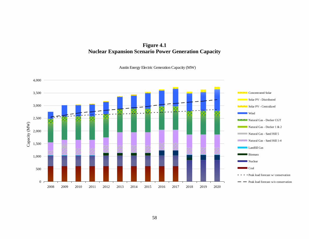
58

Figure 4.1

Nuclear Expansion Scenario Power Generation Capacity


0

500

1,000

1,500

2,000

2,500

3,000

3,500

4,000

2008 2009 2010 2011 2012 2013 2014 2015 2016 2017 2018 2019 2020

Concentrated Solar



Wind





Landfill Gas

Biomass

Nuclear

Coal



Cap

acity

(M

W)

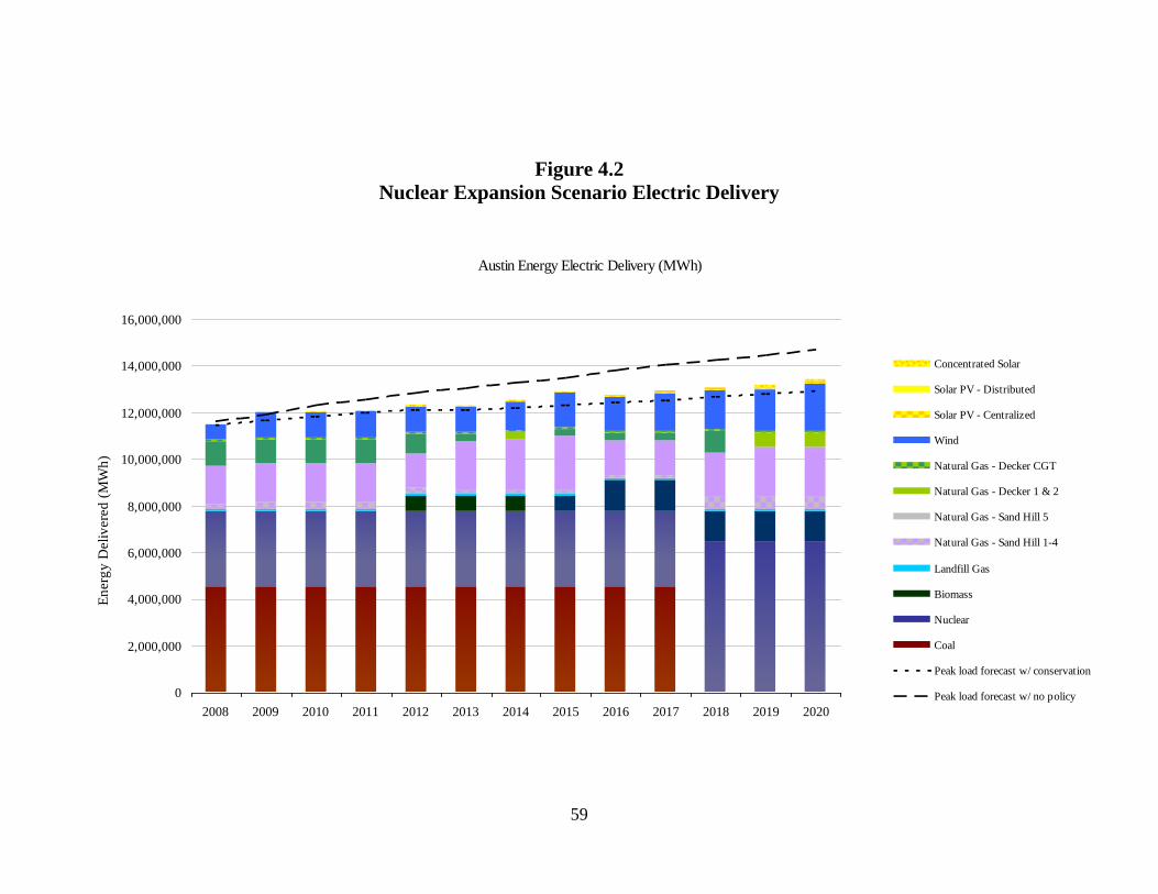
59

Figure 4.2

Nuclear Expansion Scenario Electric Delivery


0

2,000,000

4,000,000

6,000,000

8,000,000

10,000,000

12,000,000

14,000,000

16,000,000

2008 2009 2010 2011 2012 2013 2014 2015 2016 2017 2018 2019 2020

Concentrated Solar



Wind





Landfill Gas

Biomass

Nuclear

Coal



En

erg

y D

eli

vere

d (

MW

h)

60

Figure 4.3

Nuclear Expansion Scenario Hourly Load Profile (Peak Demand, Summer 2000)



0

500

1,000

1,500

2,000

2,500

3,000

3,500

4,000

0 4 8 12 16 20 24

Hour of day

Coal Nuclear




Wind Solar PV - Centralized

Solar PV - Distributed Concentrated Solar

Purchased power Peak load forecast w/o conservation


Peak

Dem

an

d (

MW

)

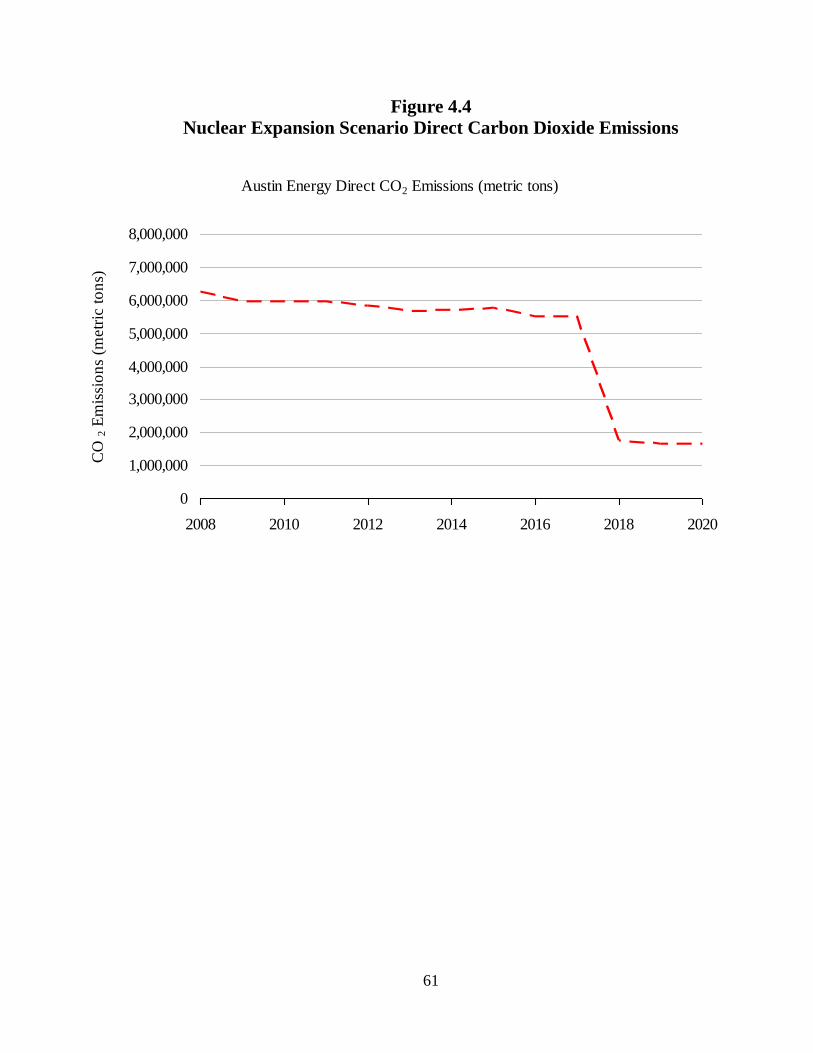
61

Figure 4.4

Nuclear Expansion Scenario Direct Carbon Dioxide Emissions


0

1,000,000

2,000,000

3,000,000

4,000,000

5,000,000

6,000,000

7,000,000

8,000,000

2008 2010 2012 2014 2016 2018 2020

CO

2 E

mis

sio

ns

(metr

ic t

on

s)

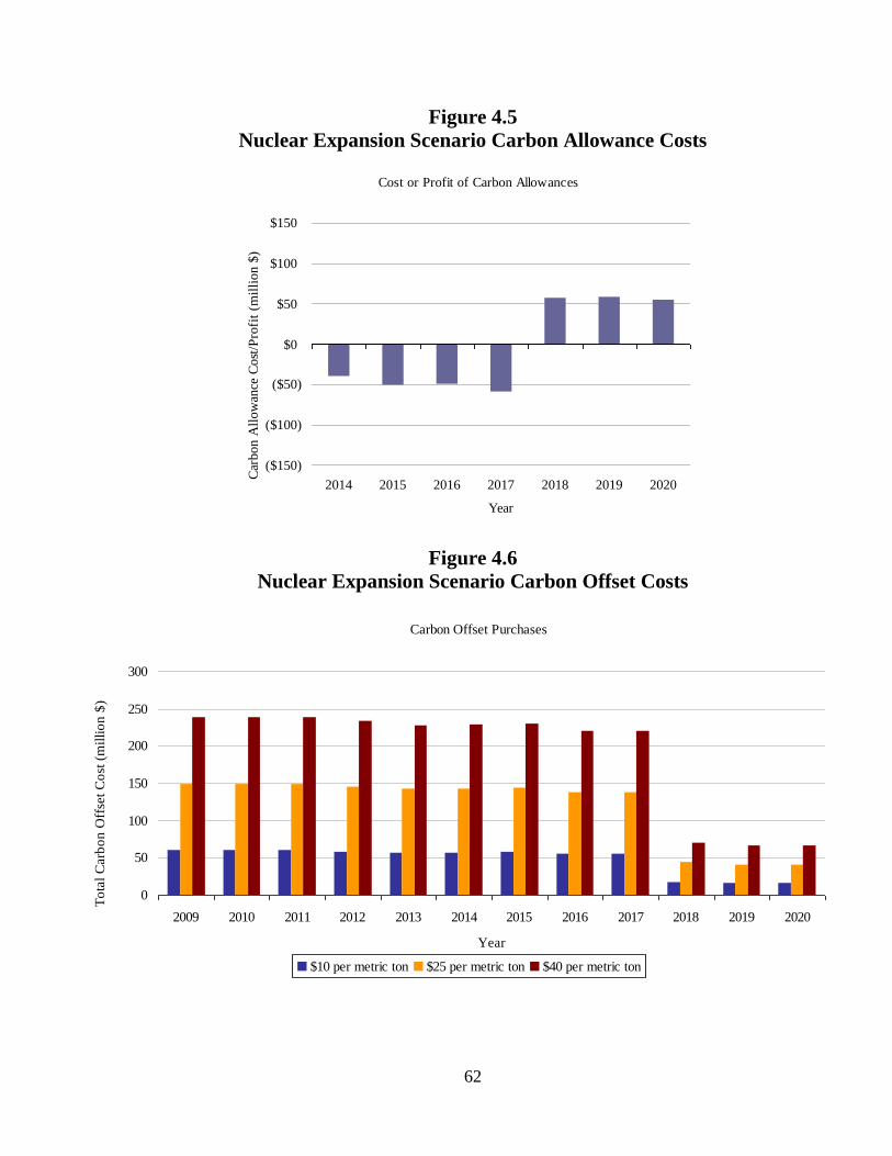
62

Figure 4.5

Nuclear Expansion Scenario Carbon Allowance Costs

Figure 4.6

Nuclear Expansion Scenario Carbon Offset Costs


($150)

($100)

($50)

$0

$50

$100

$150

2014 2015 2016 2017 2018 2019 2020

Year

Car

bon A

llow

ance

Co

st/P

rofi

t (m

illi

on $

)


0

50

100

150

200

250

300

2009 2010 2011 2012 2013 2014 2015 2016 2017 2018 2019 2020

Year


To

tal

Carb

on

Off

set

Co

st (

mil

lio

n $

)

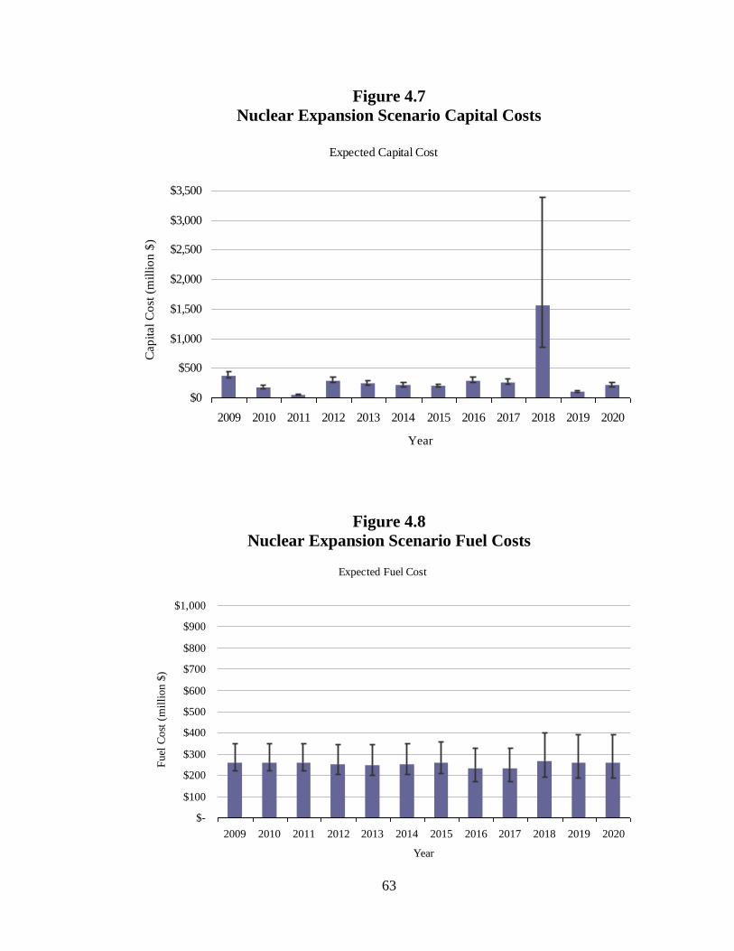
63

Figure 4.7

Nuclear Expansion Scenario Capital Costs

Figure 4.8

Nuclear Expansion Scenario Fuel Costs


$0

$500

$1,000

$1,500

$2,000

$2,500

$3,000

$3,500

2009 2010 2011 2012 2013 2014 2015 2016 2017 2018 2019 2020

Year

Cap

ital

Co

st (

mil

lio

n $

)

Expected Fuel Cost

$-

$100

$200

$300

$400

$500

$600

$700

$800

$900

$1,000

2009 2010 2011 2012 2013 2014 2015 2016 2017 2018 2019 2020

Year

Fuel

Cost

(m

illi

on $

)

64

Figure 4.9

Nuclear Expansion Scenario Levelized Costs


0

1

2

3

4

5

6

7

8

9

10

2009 2010 2011 2012 2013 2014 2015 2016 2017 2018 2019 2020

0%

10%

20%

30%

40%

50%

60%

70%

80%

90%




Wind





Landfill Gas

Biomass

Nuclear

Coal


Gen

era

tion

from

Cap

acity

Ad

ditio

ns (%

)

Ex

pecte

d I

ncre

ase

in

Lev

eli

zed

Ele

ctr

icit

y C

ost

(cen

ts/k

Wh

)

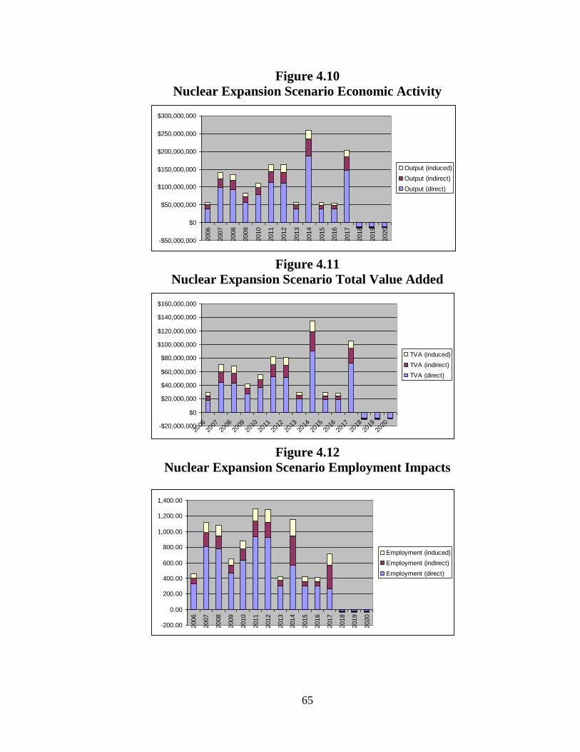
65

Figure 4.10

Nuclear Expansion Scenario Economic Activity

Figure 4.11

Nuclear Expansion Scenario Total Value Added

Figure 4.12

Nuclear Expansion Scenario Employment Impacts

-$50,000,000

$0

$50,000,000

$100,000,000

$150,000,000

$200,000,000

$250,000,000

$300,000,000

2006

2007

2008

2009

2010

2011

2012

2013

2014

2015

2016

2017

2018

2019

2020

Output (induced)

Output (indirect)

Output (direct)

-$20,000,000

$0

$20,000,000

$40,000,000

$60,000,000

$80,000,000

$100,000,000

$120,000,000

$140,000,000

$160,000,000

2006

2007

2008

2009

2010

2011

2012

2013

2014

2015

2016

2017

2018

2019

2020

TVA (induced)

TVA (indirect)

TVA (direct)

-200.00

0.00

200.00

400.00

600.00

800.00

1,000.00

1,200.00

1,400.00

2006

2007

2008

2009

2010

2011

2012

2013

2014

2015

2016

2017

2018

2019

2020



Employment (direct)

66

Chapter 5. High Renewables Scenario

The high renewable resource investment scenario evaluates the shift towards a cleaner

energy portfolio that eliminates the need for burning coal to generate electricity. details

additions to AE’s resource portfolio from 2009 to 2020 by fuel source, power generation

technology, or facility, for the proposed high renewables scenario. By eliminating the

necessity of burning coal for electricity, Austin Energy (AE) eliminates a resource that

currently accounts for 71 percent of its carbon dioxide (CO2) emissions while only

providing 32 percent of its annual energy needs. Renewable energy technologies present

a much more sustainable source of power generation than fossil fueled technologies

because they utilize resources that are not depleted during the energy conversion process

and do not emit harmful pollutants or by-products into the atmosphere and ecosystem.

The high renewables scenario presents an extreme implementation of current renewable

energy technologies to AE’s power system. The renewables power generation mix

presents an ambitious and optimistic presentation of renewable power options through

2020. Investments are made gradually in a manner that appears optimistically possible

given current and expected advancements in these technologies and expansion in Texas’

electric grid. Utility-scale solar, geothermal, and biomass facility investments are limited

to current and expected capacity constraints. Wind facilities are assumed to be

unconstrained by capacity, but in fact may have a penetration limit due to their inherent

unreliability.

Biomass and geothermal power plants can provide baseload power that is available

continuously in the same manner as coal, hydroelectric, and nuclear facilities. Therefore,

biomass and geothermal plants provide a reliable source of energy as long as supplies are

available. In addition to the biomass project that will begin operation in 2012, AE has

proposed an additional 100 MW project to come on-line in 2016. The following scenario

includes an additional 90 MW of biomass generation capacity to be added in 2020.

Although no geothermal facility currently exists in Texas, there is some potential for

geothermal power production. This scenario proposes a total of 100 MW of geothermal

energy to be added to AE’s resource portfolio with 50 MW additions occurring in 2014

and 2020, respectively. An addition of 15 MW of landfill gas power in 2016 provides an

additional source of local baseload power.

Wind and solar resources provide an intermittent source of clean energy. AE is currently

proposing an aggressive expansion of wind and solar assets (to 1,029 MW and 101 MW

of generation capacity, respectively). The high renewables scenario makes even greater

investments in wind and solar assets (to 1,990 and 913 MW of generation capacity,

respectively). Solar additions include the construction of two large-scale concentrated

solar facilities that use parabolic trough methods (the most advanced and least cost option

for concentrated solar power generation), gradual accelerated investment in local

distributed generation from solar photovoltaic (PV) panels on rooftops, and gradual

investment in centralized PV systems. Onshore wind energy investments almost double

that proposed by AE and a gradual addition of 305 MW of offshore wind power

67

generation capacity is proposed in an effort to tap into wind energy availability at hours

different from typical onshore wind availability.

System Reliability

Eliminating AE’s stake in the Fayette Power Project coal facility creates concerns

regarding system reliability, as this removes a major source of baseload power generation

(607 MW of power generation capacity). In an effort to relieve such concerns, 390 MW

of baseload power would be provided from geothermal and biomass facilities. However,

the high renewables scenario creates a resource portfolio that becomes highly dependent

upon the unreliable variable nature of wind and solar energy. Due to low capacity factors,

a system so dependent on wind and solar would require much greater power generation

capacity than forecasted demand. Figure 5.1 demonstrates that AE’s power generation

capacity would in fact greatly exceed forecasted peak load with and without conservation

goals being met. This proposed system would hold 5,227 MW of power generation

capacity compared to a system of 3,923 MW of power generation capacity under the AE

proposed energy resource plan. By 2020, 812 MW of generation capacity will be

provided from baseload power sources (nuclear, geothermal, and biomass) and 2,903

MW of power generation capacity will come from intermittent sources of energy (wind

and solar). 2,324 MW of power generation capacity will come from energy resources that

can provide continuous sources of power as long as the facility is in operation.

Figure 5.2 demonstrates that, given expected capacity factors for wind and solar (29 and

17 percent, respectively) as well as current capacity factors for AE’s nuclear and natural

gas facilities, AE will be able to reliably deliver electricity to its customers as long as AE

meets its conservation goals. It appears that AE will be able to provide reliable service

even if conservation goals are only met halfway, the same expected reliability of AE’s

proposed energy resource plan. However, because 52 percent of expected electricity

delivered is dependent upon intermittent sources of energy, there is some cause for

concern for system reliability given the chances that wind and solar do not meet expected

production levels. However, the natural gas facilities operated by AE are expected to

operate at levels much lower than capacity and would serve as reliable backup sources of

power.

To demonstrate the risks of a system highly dependent on wind and solar energy, Figure

5.3 details AE’s expected hourly load profile for the hottest day (peak demand) in the

summer of 2020. The hourly load profile follows expected solar and wind profiles and

demonstrates that AE will be able to meet peak demand without purchasing power even

on the hottest day of the summer, if expected wind and solar production is met and AE

meets its conservation goals. Since AE makes gradual additions to its resource portfolio

from baseload, intermediate, and intermittent sources of energy, it appears that AE will

be able to meet peak demand in all years between 2009 and 2020 without purchasing

power. This demonstrates that it is possible to construct a power system focused on

renewable resources to provide predominantly clean energy to customers.

68


AE’s proposed resource plan will increase the amount of clean energy power generation

capacity to about 30 percent of its entire resource portfolio by 2020, the goal set by the

Austin Climate Protection Plan. In comparison, the high renewables scenario will

increase the amount of clean energy power generation capacity to about 63 percent of

AE’s resource portfolio, more than doubling what is currently being proposed by AE.

Given expected capacity factors for wind and solar and adjusted capacity factors for

natural gas to account for forecasted demand, about 72 percent of AE’s actual power

generation would come from clean energy sources in 2020 (compared to 26 percent in

AE’s proposed resource plan). Fifty-two percent of actual electricity delivered would

come from wind and solar alone. By eliminating CO2 emissions caused by the burning of

coal and shifting to a much cleaner resource portfolio, CO2 emissions would drop

dramatically in the high renewables scenario (see Figure 5.4). AE’s CO2 emissions in

2007 were roughly 6.1 million metric tons. Under the high renewables scenario CO2

emissions would drop to under 600,000 metric tons by 2020, a reduction of almost 90

percent. The high renewables scenario demonstrates an opportunity to significantly

eliminate AE’s carbon footprint by reducing CO2 emissions to a level that makes

offsetting emissions to zero very manageable.



For example, under the Lieberman-Warner Climate Security Act of 2007, a portion of an

entity’s emissions would be accounted for by free permits, or allowances, while a portion

of allowances would be auctioned. Figure 5.5 estimates that AE could receive profits of

about $216 million from 2014 to 2020 based upon allowance price estimates for the

Lieberman-Warner bill and expected CO2 emissions under the high renewables scenario.

This compares to potential costs of about $490 million under AE’s proposed energy

resource plan.

Under the high renewables scenario, offsetting CO2 emissions to zero also becomes much

more manageable. Figure 5.6 provides a range of annual costs to offset emissions to zero,

thus effectively achieving carbon-neutrality. The costs of offsets would be dramatically

reduced in the years 2014 and 2020, respectively, as half of AE’s stake in its coal facility

would be eliminated. By 2020, annual costs would range from $6 to $23 million

compared to $58 to $230 million under AE’s proposed resource plan.

The high renewables scenario provides one of the most sustainable power generation

scenarios conceivable for AE. This future power generation mix would rely on clean

energy for almost 75 percent of customer electric needs by 2020. Natural gas facilities

would serve as backup for intermittent sources of energy and as peaking units. The

primary issue with sustainability then comes from arguments regarding the sustainable

nature of nuclear energy. Under the high renewables scenario, AE continues its operation

of just over 400 MW of power from its stake in a nuclear facility to provide baseload

power. While nuclear energy does not emit greenhouse gas (GHG) emissions or other

harmful air pollutants, there are serious issues regarding land use, hazardous waste, and

69

catastrophic risks associated with producing energy through nuclear fission. Our study

concludes that nuclear energy provides a more sustainable form of energy than coal due

to the lack of GHG emissions and thus was kept as part of AE’s resource portfolio, rather

than coal, to help ensure reliable service and affordable electric rates. As renewable

resources continue to advance, reliance on nuclear energy as well as natural gas could

become less necessary. However, given a timeframe of only 11 years, we believe that

nuclear is a necessary component to ensuring AE’s ability to provide reliable energy at

low costs under a high renewable energy resource mix.


It should first be noted that our model does not account for AE projections of the costs of

their scheduled or proposed additions to its resource portfolio. As many of these additions

come in the form of power purchase agreements or currently owned and operated facility

expansions, the following cost estimates may not coincide with AE projections. The cost

estimates provided below are based solely upon general cost estimates for new power

generation facilities.

Figure 5.7 details the capital cost estimates for the scheduled and proposed additions in

the high renewables power generation mix. Capital costs are expressed as the sum of total

overnight costs for additions scheduled in a particular year. Total expected capital costs

range from $6.9 to $9.5 billion (compared to $2.2 to $3.0 billion under AE’s proposed

resource plan). Capital costs are expressed as total overnight costs. It is important to

recognize the year for which a project is proposed. On-shore wind turbines are a mature

technology with relatively stable expected costs, but other renewable technologies

present much uncertainty in capital costs. No geothermal, concentrated solar plant, or off-

shore wind facility has ever been constructed in Texas, so cost estimates for these

facilities have larger ranges. Costs for biomass plants may rise as supplies in Texas

decrease. It is expected that costs to build utility-scale solar plants and to install solar PV

panels will drop considerably in the next decade, but when and by how much is

uncertain. In this model, costs are expressed as current estimates and ranges are

determined based upon the relative maturity of the technology and expected direction by

which costs are expected to flow.

Figure 5.8 details expected annual fuel costs for the high renewables scenario. Since the

amount of fossil-fueled resources changes dramatically under this scenario, fuel costs are

expected to drop considerably, greatly reducing the risks associated with fuel price

instability. Fuel costs are expected to decrease as coal usage is reduced and eliminated.

By 2020, fuel costs under this scenario would range from $67 to $172 million annually

(compared to $93 to $328 million under AE’s proposed resource plan).


impact of the levelized costs of new power generation resources as a percentage of

overall generation capacity. The high renewables scenario presents an almost completely

redefined power generation mix with over 75 percent actual power generation coming

from additions since 2009. Therefore, the costs of these additions will have a significant

70

impact on the costs of electricity. This model estimates that electric rates would rise by

by between 4.5 and 8 cents per kilowatt-hour of electricity consumed by 2020 under the

high renewables scenario, compared to between 1.5 and 3 cents per kilowatt-hour of

electricity consumed under AE’s proposed energy resource plan. It should be noted that

this expected increase in electric rates is based solely on new power generation

investments. Offset costs or any unexpected additional costs to the utility could also be

passed on to the customer during this time period. Additionally, the calculation for

expected increase in cost of electricity does not appoint a monetary value of reducing or

removing coal or any other resource from AE’s resource portfolio as the methods for

evaluating how much AE could receive are beyond the scope of this report. Such removal

may help to alleviate the additional costs to electricity accrued from the identified

resource additions.

The high renewable scenario represents a major increase in economic activity for the

Greater Austin Area attributed to investments in 250 MW of centralized photovoltaic

power generation facilities, 15 MW of landfill gas capacity, and 55 MW of distributed

photovoltaic power generation capacity. The most significant impact upon the local

economy would be created by the rapid acceleration in solar PV modules on rooftops.

This could create a vibrant local solar manufacturing and installation industry.

Additionally, centralized PV systems located within the Austin region could further

accelerate the solar industry in Austin.

Figure 5.10 shows the economic output in the Greater Austin Area generated by the high

renewables scenario. Local economic activity peaks above $500 million in 2016. Figure

5.11 shows the total value added to the Greater Austin Area from the investments made

in the high renewables scenario. Figure 5.12 shows the impacts on employment created

through the high renewables scenario.

71

Table 5.1

High Renewables Scenario Scheduled Additions and Subtractions to Generation Mix

2008 2009 2010 2011 2012 2013 2014 2015 2016 2017 2018 2019 2020

Coal 607 0 0 0 0 0 -305 0 0 0 0 0 -302

Nuclear 422 0 0 0 0 0 0 0 0 0 0 0 0





Wind 274 165 0 100 0 0 100 200 0 526 0 100 220

Offshore Wind 0 0 0 0 50 0 50 0 50 0 50 0 105

Biomass 0 0 0 0 100 0 0 0 100 0 0 0 90


Landfill Gas 12 0 0 0 0 0 0 0 15 0 0 0 0




IGCC w/ CCS 0 0 0 0 0 0 0 0 0 0 0 0 0

IGCC w/o CCS 0 0 0 0 0 0 0 0 0 0 0 0 0

Geothermal 0 0 0 0 0 0 50 0 0 0 50 0 0

Storage 0 0 0 0 0 0 0 0 0 0 0 0 0


Purchased Power 0 0 0 0 0 0 0 0 0 0 0 0 0


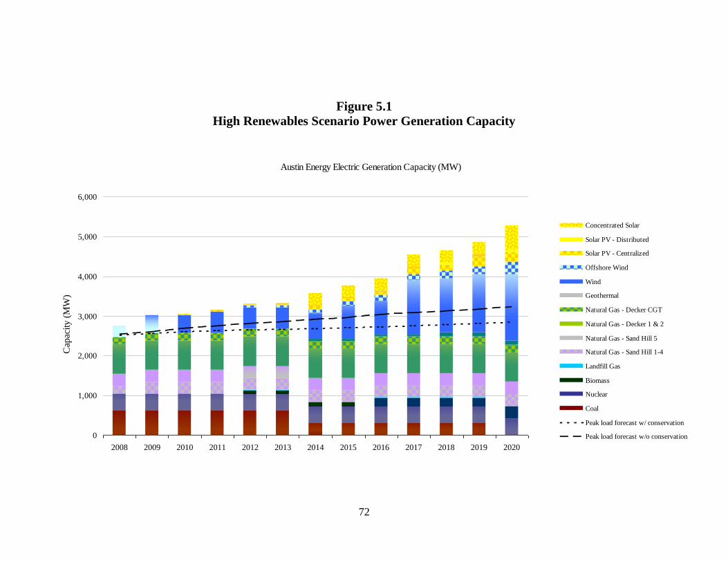
72

Figure 5.1

High Renewables Scenario Power Generation Capacity


0

1,000

2,000

3,000

4,000

5,000

6,000

2008 2009 2010 2011 2012 2013 2014 2015 2016 2017 2018 2019 2020

Concentrated Solar



Offshore Wind

Wind

Geothermal





Landfill Gas

Biomass

Nuclear

Coal



Cap

acity

(M

W)

73

Figure 5.2

High Renewables Scenario Electric Delivery


0

2,000,000

4,000,000

6,000,000

8,000,000

10,000,000

12,000,000

14,000,000

16,000,000

2008 2009 2010 2011 2012 2013 2014 2015 2016 2017 2018 2019 2020

Concentrated Solar



Offshore Wind

Wind

Geothermal





Landfill Gas

Biomass

Nuclear

Coal



En

erg

y D

eli

vere

d (

MW

h)

74

Figure 5.3

High Renewables Scenario Hourly Load Profile (Peak Demand, Summer 2000)



0

500

1,000

1,500

2,000

2,500

3,000

3,500

4,000

0 4 8 12 16 20 24

Hour of day

Coal Nuclear




Geothermal Wind

Offshore Wind Solar PV - Centralized


Peak load forecast w/o conservation Peak load forecast w/ conservation

Peak

Dem

an

d (

MW

)

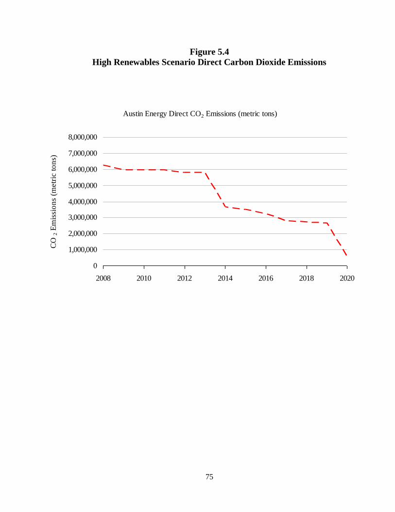
75

Figure 5.4

High Renewables Scenario Direct Carbon Dioxide Emissions


0

1,000,000

2,000,000

3,000,000

4,000,000

5,000,000

6,000,000

7,000,000

8,000,000

2008 2010 2012 2014 2016 2018 2020

CO

2 E

mis

sio

ns

(metr

ic t

on

s)

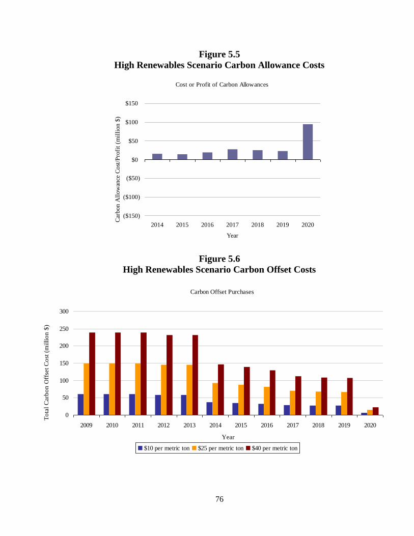
76

Figure 5.5

High Renewables Scenario Carbon Allowance Costs

Figure 5.6

High Renewables Scenario Carbon Offset Costs


($150)

($100)

($50)

$0

$50

$100

$150

2014 2015 2016 2017 2018 2019 2020

Year

Car

bon A

llow

ance

Co

st/P

rofi

t (m

illi

on $

)


0

50

100

150

200

250

300

2009 2010 2011 2012 2013 2014 2015 2016 2017 2018 2019 2020

Year


To

tal

Carb

on

Off

set

Co

st (

mil

lio

n $

)

77

Figure 5.7

High Renewables Scenario Capital Costs

Figure 5.8

High Renewables Scenario Fuel Costs


$0

$500

$1,000

$1,500

$2,000

$2,500

$3,000

2009 2010 2011 2012 2013 2014 2015 2016 2017 2018 2019 2020

Year

Cap

ital

Co

st (

mil

lio

n $

)

Expected Fuel Cost

$-

$100

$200

$300

$400

$500

$600

$700

$800

$900

$1,000

2009 2010 2011 2012 2013 2014 2015 2016 2017 2018 2019 2020

Year

Fuel

Cost

(m

illi

on $

)

78

Figure 5.9

High Renewables Scenario Levelized Costs


0

1

2

3

4

5

6

7

8

9

10

2009 2010 2011 2012 2013 2014 2015 2016 2017 2018 2019 2020

0%

10%

20%

30%

40%

50%

60%

70%

80%

90%




Offshore Wind

Wind

Geothermal





Landfill Gas

Biomass

Nuclear

Coal


Gen

era

tion

from

Cap

acity

Ad

ditio

ns (%

)

Ex

pecte

d I

ncre

ase

in

Lev

eli

zed

Ele

ctr

icit

y C

ost

(cen

ts/k

Wh

)

79

Figure 5.10

High Renewables Scenario Economic Activity

Figure 5.11

High Renewables Scenario Total Value Added

Figure 5.12

High Renewables Scenario Employment Impacts

$0

$100,000,000

$200,000,000

$300,000,000

$400,000,000

$500,000,000

$600,000,000

2006

2007

2008

2009

2010

2011

2012

2013

2014

2015

2016

2017

2018

2019

2020

Output (induced)

Output (indirect)

Output (direct)

$0

$50,000,000

$100,000,000

$150,000,000

$200,000,000

$250,000,000

$300,000,000

2006

2007

2008

2009

2010

2011

2012

2013

2014

2015

2016

2017

2018

2019

2020

TVA (induced)

TVA (indirect)

TVA (direct)

0.00

500.00

1,000.00

1,500.00

2,000.00

2,500.00

3,000.00

3,500.00

4,000.00

4,500.00

2006

2007

2008

2009

2010

2011

2012

2013

2014

2015

2016

2017

2018

2019

2020



Employment (direct)

80

Chapter 6. Expected Renewables Scenario

The expected renewable resource investment scenario is a compromise between Austin

Energy’s (AE) proposed resource plan and the high renewable resource scenario. details

the proposed additions to AE’s resource portfolio from 2009 to 2020. The scenario

presents a schedule of investments in power generating capacity that is considered more

realistic than the high renewables scenario in regards to both affordability and

practicality. In this scenario, AE eliminates half of its stake in the Fayette Power Project

(FPP) in 2018, thus halving its CO2 emissions attributed to the burning of coal. To make

up for lost coal baseload power, AE maintains the schedule of 572 MW of wind, 300

MW of natural gas, and 200 MW of baseload biomass additions included in AE’s

proposed resource plan. AE would make greater investments in solar through 2020 than

what is included in the original resource plan (341 MW versus 100 MW) under this

scenario, but invests in about two-thirds less than the solar investments scheduled in the

high renewables scenario. In addition to the currently scheduled 30 MW centralized solar

installation expected to be available by 2010, AE would install two 50 MW centralized

solar photovoltaic (PV) facilities, one in 2014 and another in 2019. AE would install two

100 MW concentrating parabolic trough solar facilities, one in 2014 and the other in

2020. This scenario relies on the assumption that distributed solar PV would be installed

at a rate of 1 MW per year, beginning in 2010 (considering a typical residential

installation is about 3 kW and 1 MW = 1,000 kW, this would mean the installation of

about 333 residential PV systems per year). Unlike the high renewables scenario, this

scenario does not include the addition of any geothermal or offshore wind sources, as

AE’s access to these resources is limited geographically.

System Reliability

Figure 6.1 demonstrates that AE’s power generation capacity would exceed forecasted

peak load with and without conservation goals being met. Eliminating about half of AE’s

stake in FPP creates concerns regarding system reliability, as this removes a major source

of baseload power generation (305 MW). In an effort to relieve such concerns, biomass

facilities would provide 200 MW of baseload power. However, the expected renewables

scenario creates a resource portfolio that becomes highly dependent upon the unreliable

variable nature of wind and solar energy, as well as greater natural gas consumption. Due

to low capacity factors and the probabilistic possibility of failure, a system so dependent

on wind and solar would require much greater power generation capacity than forecasted

demand. Beginning in 2018 with the removal of half of FPP, the combination of baseload

and natural gas sources cannot meet demand by themselves in the presence of a failure of

wind or solar. This reliance on variable wind and solar resources introduces a real

concern of potential system failures.

This proposed system would hold 3,659 MW of power generation capacity compared to a

system of 3,923 MW of generation capacity under the AE proposed energy resource plan.

By 2020, 924 MW of power generation capacity will be provided from baseload power

81

sources (coal, nuclear, and biomass) and 1,188 MW of power generation capacity will

come from variable energy sources (wind and solar).



gas facilities, AE will be able to deliver electricity to its customers as long as AE meets

its conservation goals. If wind and solar do not meet expected production levels, the

natural gas facilities would serve as backup sources of power. By 2020, combined cycle

natural gas units at Sand Hill would be providing close to baseload levels of electricity

because of the lower CO2 emissions associated with them, while the other natural gas

units at Sand Hill and Decker act as peaking and reserve capacity.

Figure 6.3 details AE’s expected hourly load profile for the hottest day (peak demand

day) in the summer of 2020. The hourly load profile follows expected solar and wind

profiles, and demonstrates that AE will most likely have to purchase power to be able to

meet peak demand in 2020 even if AE meets its conservation goals. At peak, with all the

natural gas facilities operating at full capacity, AE will still have to purchase 185 MW

from the grid. An additional 200 MW natural gas facility could make up this difference if

AE so chose.



capacity to about 30 percent of its entire resource portfolio by 2020, the goal set by the

Austin Climate Protection Plan. In comparison, the expected available renewables

scenario will increase the amount of renewable power generating capacity to about 38

percent of AE’s entire resource portfolio. Given expected capacity factors for wind and

solar and adjusted capacity factors for natural gas to account for forecasted demand,

about 33 percent of AE’s actual power generation would come from clean energy sources

in 2020 (compared to 26 percent in AE’s proposed resource plan) with 22 percent of

actual electricity delivered coming from wind and solar. By eliminating half of the CO2

emissions caused by the burning of coal, CO2 emissions would decrease by about 36

percent from 2008 levels in the expected renewables scenario (see Figure 6.4). The

expected renewables scenario demonstrates an opportunity to reduce AE’s carbon

footprint substantially by 2020 with seemingly reasonable investments in additional low-

carbon facilities. Although this scenario would result in the production of lower CO2

emissions, Figure 6.6 estimates that AE would still have to pay between $29 and $48

million annually based upon carbon allowance price estimates if the Lieberman-Warner

bill were to be implemented. This compares to potential annual costs of about $47 to $96

million under AE’s proposed energy resource plan.

Under the expected renewables scenario, offsetting CO2 emissions to zero becomes more

manageable than in the proposed resource plan. Figure 6.6 provides a range of annual

costs to offset emissions to zero, thus effectively achieving carbon-neutrality. By 2020,

the annual costs for offsets would range from $40 to $160 million compared to $58 to

$230 million under AE’s proposed resource plan.

82

The expected renewables scenario provides a modest increase in renewable and low-

carbon generating facilities over those included in the proposed resource plan. This

power generation mix reveals practical steps toward AE’s pursuit of carbon neutrality by

2020 without a tremendous cost increase over the proposed resource plan. As CO2

emissions decline in this scenario, the issue with sustainability comes from arguments

regarding the sustainable nature of nuclear energy. Under the expected renewables

scenario, AE continues its operation of just over 400 MW of power from its stake in a

nuclear facility to continue to provide baseload power. While nuclear energy does not

emit greenhouse gases or other harmful air pollutants, there are serious issues regarding

land use, hazardous waste, and catastrophic risks associated with producing energy

through nuclear fission. However, given a timeframe of only 11 years, we believe that

nuclear is a necessary component to ensuring AE’s ability to provide reliable energy at

low costs under a more renewable energy resource mix.


Figure 6.7 details the capital cost estimates for AE’s scheduled and proposed additions to

its power generation mix. Expected capital costs range from $2.6 to $3.7 billion

(compared to $2.2 to $3.0 billion under AE’s proposed resource plan). Capital costs are

expressed as total overnight costs. Therefore, it is important to recognize the year for

which a project is proposed. In this model, costs are expressed as current estimates and

ranges are determined based upon the relative maturity of the technology and expected

direction by which costs are expected to flow.

Figure 6.8 details annual fuel costs for the high renewables scenario. Fuel costs are not

expected to decrease because, even though the elimination of half of FPP will reduce coal

consumption, that resource is replaced by natural gas and biomass that is typically more

expensive. Fuel costs would, by 2020 under this scenario, range from $205 to $413

million annually (compared to $93 to $328 million under AE’s proposed resource plan).

Figure 6.9 estimates the rise in costs on electric bills by calculating the impact of the

levelized costs of new power generation resources as a percentage of overall power

generation capacity. The expected renewables scenario presents a modestly redefined

power generation mix with about 30 percent of actual power generation coming from

additions since 2009. Since this scenario is similar to the proposed resource plan, the

expected costs of these additions will not have a significantly different impact on the

costs of electricity. This model estimates that the cost to produce electricity would rise

between 1.8 and 3.2 cents per kilowatt-hour (compared to between 1.5 and 3 cents per

kilowatt-hour under AE’s proposed energy resource plan). It should be noted that this

expected increase in electric rates is based solely on new power generation investments.

Offset costs or any unexpected additional costs to the utility could also be passed on to

the customer during this time period.

Figure 6.10 shows that there would be a major spike in economic activity during the

years 2011 to 2013 of over $250 million each year created by the addition of 200 MW of

natural gas power generation capacity at Sand Hill in 2013 and 50 MW of centralized

83

solar capacity in 2014. Figure 6.11 shows the total value added to the Greater Austin

Area from the investments made in the expected renewables scenario. Figure 6.12 shows

the impacts on employment created or eliminated by the expected renewables scenario.

The consequence of employment losses created from AE’s divestment in coal in the

Greater Austin Area under this scenario is an enduring relative loss of output and no net

gain of jobs.






84

Table 6.1

High Renewables Scenario Scheduled Additions and Subtractions to Generation Mix

2008 2009 2010 2011 2012 2013 2014 2015 2016 2017 2018 2019 2020

Coal 607 0 0 0 0 0 0 0 0 0 -305 0 0

Nuclear 422 0 0 0 0 0 0 0 0 0 0 0 0





Wind 274 165 0 23 0 0 50 100 0 74 0 50 110

Offshore Wind 0 0 0 0 0 0 0 0 0 0 0 0 0

Biomass 0 0 0 0 100 0 0 0 100 0 0 0 0


Landfill Gas 12 0 0 0 0 0 0 0 0 0 0 0 0




IGCC w/ CCS 0 0 0 0 0 0 0 0 0 0 0 0 0

IGCC w/o CCS 0 0 0 0 0 0 0 0 0 0 0 0 0

Geothermal 0 0 0 0 0 0 0 0 0 0 0 0 0

Storage 0 0 0 0 0 0 0 0 0 0 0 0 0


Purchased Power 0 0 0 0 0 0 0 0 0 0 0 0 0


85

Figure 6.1

Expected Renewables Scenario Power Generation Capacity


0

500

1,000

1,500

2,000

2,500

3,000

3,500

4,000

2008 2009 2010 2011 2012 2013 2014 2015 2016 2017 2018 2019 2020

Concentrated Solar



Wind





Landfill Gas

Biomass

Nuclear

Coal



Cap

acity

(M

W)

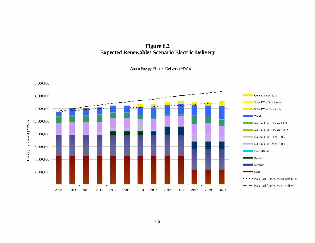
86

Figure 6.2

Expected Renewables Scenario Electric Delivery


0

2,000,000

4,000,000

6,000,000

8,000,000

10,000,000

12,000,000

14,000,000

16,000,000

2008 2009 2010 2011 2012 2013 2014 2015 2016 2017 2018 2019 2020

Concentrated Solar



Wind





Landfill Gas

Biomass

Nuclear

Coal



En

erg

y D

eli

vere

d (

MW

h)

87

Figure 6.3

Expected Renewables Scenario Hourly Load Profile (Peak Demand, Summer 2000)



0

500

1,000

1,500

2,000

2,500

3,000

3,500

4,000

0 4 8 12 16 20 24

Hour of day

Coal Nuclear








Peak

Dem

an

d (

MW

)

88

Figure 6.4

Expected Renewables Scenario Direct Carbon Dioxide Emissions


0

1,000,000

2,000,000

3,000,000

4,000,000

5,000,000

6,000,000

7,000,000

8,000,000

2008 2010 2012 2014 2016 2018 2020

CO

2 E

mis

sio

ns

(metr

ic t

on

s)

89

Figure 6.5

Expected Renewables Scenario Carbon Allowance Costs

Figure 6.6

Expected Renewables Scenario Carbon Offset Costs


($150)

($100)

($50)

$0

$50

$100

$150

2014 2015 2016 2017 2018 2019 2020

Year

Car

bon A

llow

ance

Co

st/P

rofi

t (m

illi

on $

)


0

50

100

150

200

250

300

2009 2010 2011 2012 2013 2014 2015 2016 2017 2018 2019 2020

Year


To

tal

Carb

on

Off

set

Co

st (

mil

lio

n $

)

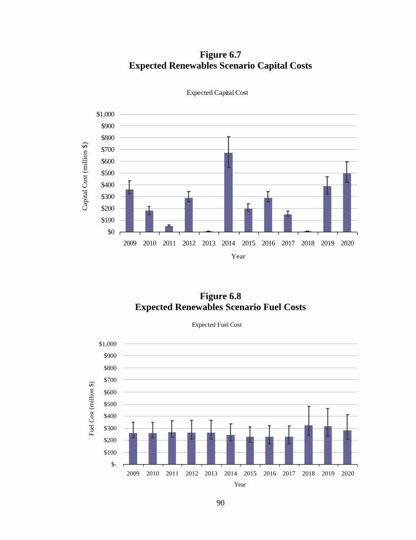
90

Figure 6.7

Expected Renewables Scenario Capital Costs

Figure 6.8

Expected Renewables Scenario Fuel Costs


$0

$100

$200

$300

$400

$500

$600

$700

$800

$900

$1,000

2009 2010 2011 2012 2013 2014 2015 2016 2017 2018 2019 2020

Year

Cap

ital

Co

st (

mil

lio

n $

)

Expected Fuel Cost

$-

$100

$200

$300

$400

$500

$600

$700

$800

$900

$1,000

2009 2010 2011 2012 2013 2014 2015 2016 2017 2018 2019 2020

Year

Fuel

Cost

(m

illi

on $

)

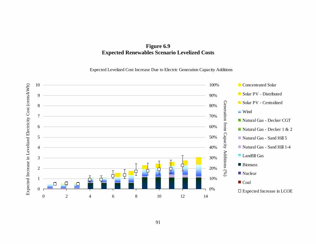
91

Figure 6.9

Expected Renewables Scenario Levelized Costs


0

1

2

3

4

5

6

7

8

9

10

0 2 4 6 8 10 12 14

0%

10%

20%

30%

40%

50%

60%

70%

80%

90%




Wind





Landfill Gas

Biomass

Nuclear

Coal


Gen

era

tion

from

Cap

acity

Ad

ditio

ns (%

)

Ex

pecte

d I

ncre

ase

in

Lev

eli

zed

Ele

ctr

icit

y C

ost

(cen

ts/k

Wh

)

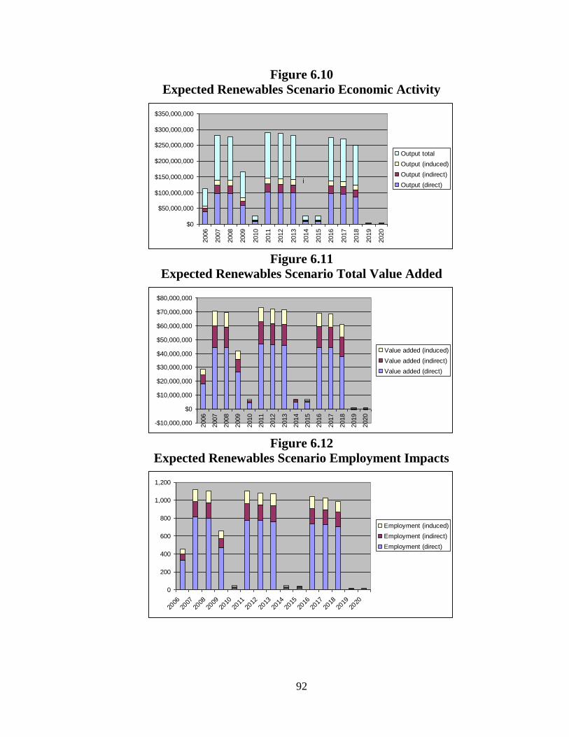
92

Figure 6.10

Expected Renewables Scenario Economic Activity

Figure 6.11

Expected Renewables Scenario Total Value Added

Figure 6.12

Expected Renewables Scenario Employment Impacts

$0

$50,000,000

$100,000,000

$150,000,000

$200,000,000

$250,000,000

$300,000,000

$350,000,000

2006

2007

2008

2009

2010

2011

2012

2013

2014

2015

2016

2017

2018

2019

2020

Output total

Output (induced)

Output (indirect)

Output (direct)i

-$10,000,000

$0

$10,000,000

$20,000,000

$30,000,000

$40,000,000

$50,000,000

$60,000,000

$70,000,000

$80,000,000

2006

2007

2008

2009

2010

2011

2012

2013

2014

2015

2016

2017

2018

2019

2020




0

200

400

600

800

1,000

1,200

2006

2007

2008

2009

2010

2011

2012

2013

2014

2015

2016

2017

2018

2019

2020



Employment (direct)

93

Chapter 7. Expected Renewables with Energy Storage

Scenario

This scenario incorporates possible energy storage capacity into the expected available

renewable resources scenario. Table 7.1 details the proposed additions to AE’s resource

portfolio from 2009 to 2020. This scenario strives to address the two primary failings of

the expected renewables scenario; a failure to meet the peak daily demand by 200 MW

and the necessity to promulgate the use of a portion of AE’s coal resources (302 MW).

To address the peak shortage and to attempt to lower carbon emissions further, this

scenario introduces 350 MW of Compressed Air Energy Storage (CAES) facility

additions through 2020 (represented as Wind + CAES in the model). CAES was

identified as the most likely storage technology because it has the lowest capital costs of

any practical and proven utility-scale storage option. In principle, pumped storage on the

Colorado River could be used as a form of energy source, but AE has yet to discuss such

an option with the Lower Colorado River Authority. Upon selecting CAES, the decision

was made to pair the compressed air storage technology with a power generation

technology. Since Austin is in a hot climate, where electricity demand peaks during

afternoons in the summer, when solar output is producing near its maximum and wind is

producing near its minimum, CAES is paired with wind facilities to achieve maximum

marginal gains. This system was designed to allow CAES to capture some excess

nighttime electricity generated by its paired wind facilities. This allows the void during

the peak afternoons and evenings to be filled by stored electricity from wind and CAES.

System Reliability


peak load with and without conservation goals being met. Under this scenario AE would

be able to eliminate all of its use of coal, rather than only half which was the limitation

experienced by the expected renewables scenario without storage. Eliminating AE’s stake

in the Fayette Power Project (FPP) coal facility creates concerns regarding system

reliability as this removes a major source of baseload power generation capacity (607

MW). In an effort to relieve some such concerns, biomass facilities would provide 200

MW of baseload power and natural gas would be used more often as base and

intermediate providers. The expected renewables with storage scenario creates a resource

portfolio that becomes highly dependent upon the unreliable variable nature of wind and

solar energy, but the addition of 350 MW of energy storage capacity will help alleviate

some of these concerns. Due to low capacity factors and the probabilistic possibility of

failure, a system so dependent on wind and solar would require much greater power

generation capacity than forecasted demand. Beginning in 2016 with the removal of half

of FPP, the combination of baseload and natural gas sources cannot meet demand by

themselves in the presence of a failure of wind or solar. This reliance on intermittent

wind and solar sources introduces a real concern of potential system failures. It should be

noted that CAES is not considered an actual power generation technology, as it simply

uses some natural gas to transfer electricity from one time of day to another, with an

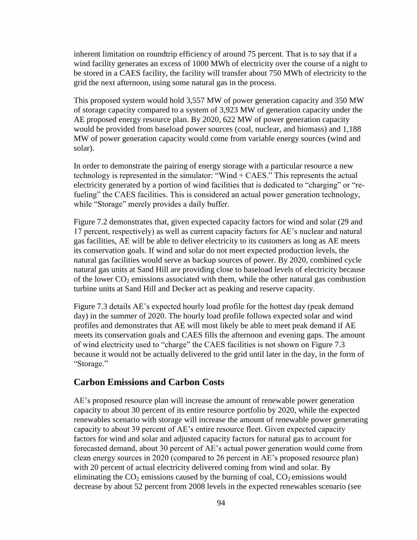
94

inherent limitation on roundtrip efficiency of around 75 percent. That is to say that if a

wind facility generates an excess of 1000 MWh of electricity over the course of a night to

be stored in a CAES facility, the facility will transfer about 750 MWh of electricity to the

grid the next afternoon, using some natural gas in the process.

This proposed system would hold 3,557 MW of power generation capacity and 350 MW

of storage capacity compared to a system of 3,923 MW of generation capacity under the

AE proposed energy resource plan. By 2020, 622 MW of power generation capacity

would be provided from baseload power sources (coal, nuclear, and biomass) and 1,188

MW of power generation capacity would come from variable energy sources (wind and

solar).

In order to demonstrate the pairing of energy storage with a particular resource a new

technology is represented in the simulator: “Wind + CAES.” This represents the actual

electricity generated by a portion of wind facilities that is dedicated to “charging” or “re-

fueling” the CAES facilities. This is considered an actual power generation technology,

while “Storage” merely provides a daily buffer.



gas facilities, AE will be able to deliver electricity to its customers as long as AE meets

its conservation goals. If wind and solar do not meet expected production levels, the

natural gas facilities would serve as backup sources of power. By 2020, combined cycle

natural gas units at Sand Hill are providing close to baseload levels of electricity because

of the lower CO2 emissions associated with them, while the other natural gas combustion

turbine units at Sand Hill and Decker act as peaking and reserve capacity.

Figure 7.3 details AE’s expected hourly load profile for the hottest day (peak demand

day) in the summer of 2020. The hourly load profile follows expected solar and wind

profiles and demonstrates that AE will most likely be able to meet peak demand if AE

meets its conservation goals and CAES fills the afternoon and evening gaps. The amount

of wind electricity used to “charge” the CAES facilities is not shown on Figure 7.3

because it would not be actually delivered to the grid until later in the day, in the form of

“Storage.”



capacity to about 30 percent of its entire resource portfolio by 2020, while the expected

renewables scenario with storage will increase the amount of renewable power generating

capacity to about 39 percent of AE’s entire resource fleet. Given expected capacity

factors for wind and solar and adjusted capacity factors for natural gas to account for

forecasted demand, about 30 percent of AE’s actual power generation would come from

clean energy sources in 2020 (compared to 26 percent in AE’s proposed resource plan)

with 20 percent of actual electricity delivered coming from wind and solar. By

eliminating the CO2 emissions caused by the burning of coal, CO2 emissions would

decrease by about 52 percent from 2008 levels in the expected renewables scenario (see

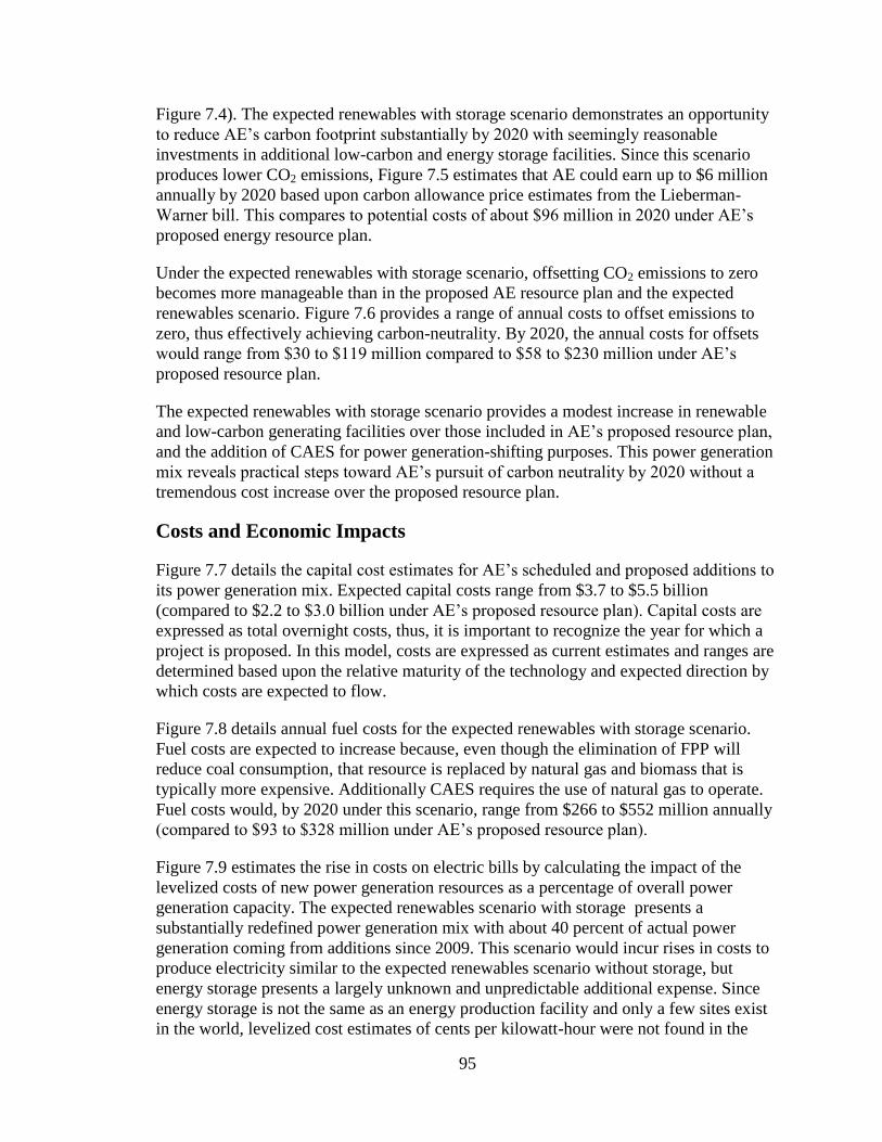
95

Figure 7.4). The expected renewables with storage scenario demonstrates an opportunity

to reduce AE’s carbon footprint substantially by 2020 with seemingly reasonable

investments in additional low-carbon and energy storage facilities. Since this scenario

produces lower CO2 emissions, Figure 7.5 estimates that AE could earn up to $6 million

annually by 2020 based upon carbon allowance price estimates from the Lieberman-

Warner bill. This compares to potential costs of about $96 million in 2020 under AE’s

proposed energy resource plan.

Under the expected renewables with storage scenario, offsetting CO2 emissions to zero

becomes more manageable than in the proposed AE resource plan and the expected

renewables scenario. Figure 7.6 provides a range of annual costs to offset emissions to

zero, thus effectively achieving carbon-neutrality. By 2020, the annual costs for offsets

would range from $30 to $119 million compared to $58 to $230 million under AE’s

proposed resource plan.

The expected renewables with storage scenario provides a modest increase in renewable

and low-carbon generating facilities over those included in AE’s proposed resource plan,

and the addition of CAES for power generation-shifting purposes. This power generation

mix reveals practical steps toward AE’s pursuit of carbon neutrality by 2020 without a

tremendous cost increase over the proposed resource plan.


Figure 7.7 details the capital cost estimates for AE’s scheduled and proposed additions to

its power generation mix. Expected capital costs range from $3.7 to $5.5 billion

(compared to $2.2 to $3.0 billion under AE’s proposed resource plan). Capital costs are

expressed as total overnight costs, thus, it is important to recognize the year for which a

project is proposed. In this model, costs are expressed as current estimates and ranges are

determined based upon the relative maturity of the technology and expected direction by

which costs are expected to flow.

Figure 7.8 details annual fuel costs for the expected renewables with storage scenario.

Fuel costs are expected to increase because, even though the elimination of FPP will

reduce coal consumption, that resource is replaced by natural gas and biomass that is

typically more expensive. Additionally CAES requires the use of natural gas to operate.

Fuel costs would, by 2020 under this scenario, range from $266 to $552 million annually

(compared to $93 to $328 million under AE’s proposed resource plan).



generation capacity. The expected renewables scenario with storage presents a

substantially redefined power generation mix with about 40 percent of actual power

generation coming from additions since 2009. This scenario would incur rises in costs to

produce electricity similar to the expected renewables scenario without storage, but

energy storage presents a largely unknown and unpredictable additional expense. Since

energy storage is not the same as an energy production facility and only a few sites exist

in the world, levelized cost estimates of cents per kilowatt-hour were not found in the

96

literature. Instead, the “cost of generation” model used by the California Energy

Commission was obtained and inputs were varied to get a rough estimate of how much

CAES would likely add to the cost of producing electricity. Since CAES is paired with

wind facilities in this scenario, we defined a new generation technology in the model –

“Wind + CAES.” We simply added the overnight costs and estimated fuel costs from

CAES alone (the only values found in literature) to the inputs values for wind facilities

alone. Fuel costs were estimated using a heat rate of CAES of 4000 BTU/kWh (about

half that of natural gas facilities alone) and a hypothetical value of CAES producing 15

percent of the time that the wind facility is actually producing. The cost model produced

levelized cost estimates of Wind + CAES at about 45 to 55 percent higher than wind

alone. With this limited information, the cost estimates associated with this scenario

should be taken as rougher estimates than the rest of the scenarios.

The simulation estimates that the cost to produce electricity would rise between 2.9 and

4.9 cents per kilowatt-hour under this scenario, compared to 1.8 and 3.2 cents per

kilowatt-hour in the expected renewables scenario without storage and compared to

between 1.5 and 3 cents per kilowatt-hour under AE’s proposed energy resource plan. It

should be noted that this expected increase in electric rates is based solely on new

investments. Offset costs or any unexpected additional costs to the utility could also be

passed on to the customer during this time period. Additionally, the calculation for

expected increase in cost of electricity does not appoint a monetary value of reducing or

removing coal or any other resource from AE’s resource portfolio as the methods for

evaluating how much AE could receive are beyond the scope of this report. Such removal

may help to alleviate the additional costs to electricity accrued from the identified

resource additions.

Figure 7.10 shows that there would be a major spike in economic activity during the

years 2011 to 2013 of over $250 million each year created by the addition of 200 MW of

natural gas power generation capacity at Sand Hill in 2013 and 50 MW of centralized

solar capacity in 2014. Figure 7.11 shows the total value added to the Greater Austin

Area from the investments made in the expected renewables scenario. Figure 7.12 shows

the impacts on employment created or eliminated by the expected renewables scenario.

The consequence of employment losses created from AE’s divestment in coal in the

Greater Austin Area under this scenario is an enduring relative loss of output and no net

gain of jobs.






97

Table 7.1

Expected Renewables with Storage Scenario Scheduled Additions and Subtractions to Generation Mix

2008 2009 2010 2011 2012 2013 2014 2015 2016 2017 2018 2019 2020

Coal 607 0 0 0 0 0 0 0 -305 0 0 0 -302

Nuclear 422 0 0 0 0 0 0 0 0 0 0 0 0





Wind 274 165 0 23 0 0 0 0 0 24 0 0 10

Wind + CAES 0 0 0 0 0 0 50 100 0 50 0 50 100

Biomass 0 0 0 0 100 0 0 0 100 0 0 0 0


Landfill Gas 12 0 0 0 0 0 0 0 0 0 0 0 0




IGCC w/ CCS 0 0 0 0 0 0 0 0 0 0 0 0 0

IGCC w/o CCS 0 0 0 0 0 0 0 0 0 0 0 0 0

Geothermal 0 0 0 0 0 0 0 0 0 0 0 0 0

Storage 0 0 0 0 0 0 50 100 0 50 0 50 100


Purchased Power 0 0 0 0 0 0 0 0 0 0 0 0 0


98

Figure 7.1

Expected Renewables with Storage Scenario Power Generation Capacity


0

500

1,000

1,500

2,000

2,500

3,000

3,500

4,000

2008 2009 2010 2011 2012 2013 2014 2015 2016 2017 2018 2019 2020

Concentrated Solar



Wind + CAES

Wind





Landfill Gas

Biomass

Nuclear

Coal



Cap

acity

(M

W)

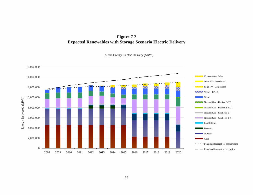
99

Figure 7.2

Expected Renewables with Storage Scenario Electric Delivery


0

2,000,000

4,000,000

6,000,000

8,000,000

10,000,000

12,000,000

14,000,000

16,000,000

2008 2009 2010 2011 2012 2013 2014 2015 2016 2017 2018 2019 2020

Concentrated Solar



Wind + CAES

Wind





Landfill Gas

Biomass

Nuclear

Coal



En

erg

y D

eli

vere

d (

MW

h)

100

Figure 7.3

Expected Renewables with Storage Scenario Hourly Load Profile (Peak Demand, Summer 2000)



0

500

1,000

1,500

2,000

2,500

3,000

3,500

4,000

0 4 8 12 16 20 24

Hour of day

Coal Nuclear






Storage Peak load forecast w/o conservation


Peak

Dem

an

d (

MW

)

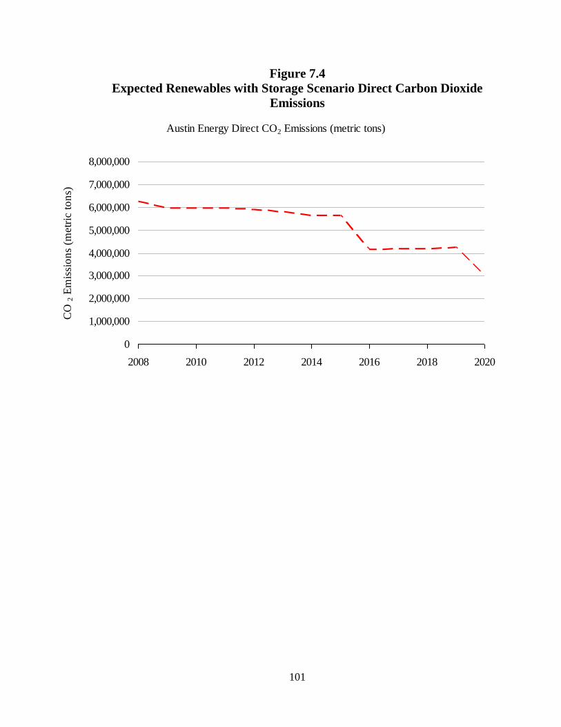
101

Figure 7.4

Expected Renewables with Storage Scenario Direct Carbon Dioxide

Emissions


0

1,000,000

2,000,000

3,000,000

4,000,000

5,000,000

6,000,000

7,000,000

8,000,000

2008 2010 2012 2014 2016 2018 2020

CO

2 E

mis

sio

ns

(metr

ic t

on

s)

102

Figure 7.5

Expected Renewables with Storage Scenario Carbon Allowance Costs

Figure 7.6

Expected Renewables with Storage Scenario Carbon Offset Costs


($150)

($100)

($50)

$0

$50

$100

$150

2014 2015 2016 2017 2018 2019 2020

Year

Car

bon A

llow

ance

Co

st/P

rofi

t (m

illi

on $

)


0

50

100

150

200

250

300

2009 2010 2011 2012 2013 2014 2015 2016 2017 2018 2019 2020

Year


To

tal

Carb

on

Off

set

Co

st (

mil

lio

n $

)

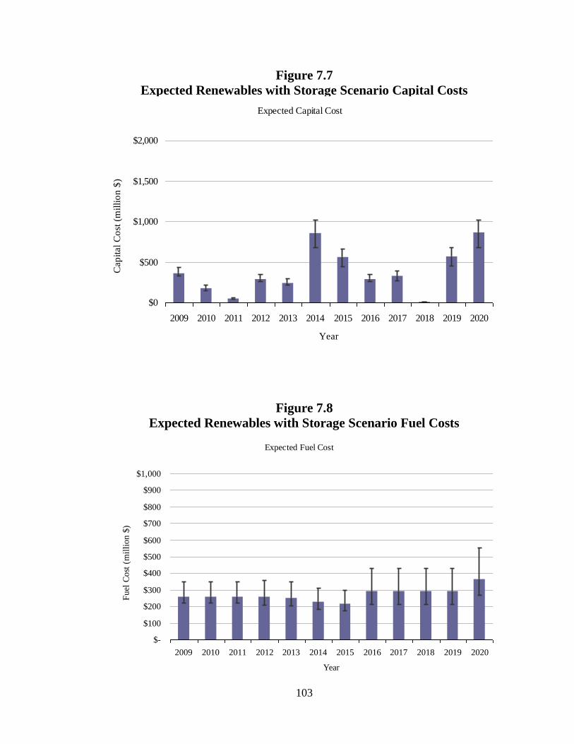
103

Figure 7.7

Expected Renewables with Storage Scenario Capital Costs

Figure 7.8

Expected Renewables with Storage Scenario Fuel Costs


$0

$500

$1,000

$1,500

$2,000

2009 2010 2011 2012 2013 2014 2015 2016 2017 2018 2019 2020

Year

Cap

ital

Co

st (

mil

lio

n $

)

Expected Fuel Cost

$-

$100

$200

$300

$400

$500

$600

$700

$800

$900

$1,000

2009 2010 2011 2012 2013 2014 2015 2016 2017 2018 2019 2020

Year

Fuel

Cost

(m

illi

on $

)

104

Figure 7.9

Expected Renewables with Storage Scenario Levelized Costs


0

1

2

3

4

5

6

7

8

9

10

2009 2010 2011 2012 2013 2014 2015 2016 2017 2018 2019 2020

0%

10%

20%

30%

40%

50%

60%

70%

80%

90%

100% Storage

Concentrated Solar



Wind + CAES

Wind





Landfill Gas

Biomass

Nuclear

Coal


Gen

era

tion

from

Cap

acity

Ad

ditio

ns (%

)

Ex

pecte

d I

ncre

ase

in

Lev

eli

zed

Ele

ctr

icit

y C

ost

(cen

ts/k

Wh

)

105

Figure 7.10

Expected Renewables with Storage Scenario Economic Activity

Figure 7.11

Expected Renewables with Storage Scenario Total Value Added

Figure 7.12

Expected Renewables with Storage Scenario Employment Impacts

-$50,000,000

$0

$50,000,000

$100,000,000

$150,000,000

$200,000,000

$250,000,000

$300,000,000

2006

2007

2008

2009

2010

2011

2012

2013

2014

2015

2016

2017

2018

2019

2020

Output (induced)

Output (indirect)

Output (direct)

-$20,000,000

$0

$20,000,000

$40,000,000

$60,000,000

$80,000,000

$100,000,000

$120,000,000

$140,000,000

2006

2007

2008

2009

2010

2011

2012

2013

2014

2015

2016

2017

2018

2019

2020




-$500

$0

$500

$1,000

$1,500

$2,000

$2,500

2006

2007

2008

2009

2010

2011

2012

2013

2014

2015

2016

2017

2018

2019

2020



Employment (direct)

106

Chapter 8. Natural Gas Expansion Scenario

The natural gas expansion scenario aligns with Austin Energy’s (AE) proposed energy

resource plan while replacing all of AE’s coal resources with natural gas by 2016. The

natural gas expansion scenario represents a strategy of replacing the burning of coal in

AE’s resource portfolio with the burning of natural gas through an expansion of its

currently existing natural gas facilities. This scenario does not entirely account for

possible limitations in expanding AE’s natural gas facilities, but does consider some

information on the capability of expansion at these facilities. Table 8.1 details the

schedule of additions and subtractions to AE’s resource portfolio by fuel source, power

generation technology, or facility, for the proposed natural gas expansion scenario. While

natural gas is a carbon emitter, it is not nearly as carbon-intensive as coal.

System Reliability

The loss of coal baseload power under this scenario raises significant concerns regarding

the reliability of AE’s system. Under this scenario the loss of 607 MW of coal baseload

power generation capacity is compensated for by the addition of natural gas and biomass.

Currently, AE uses natural gas power generation as an intermediate power source. Under

this scenario a portion of natural gas capacity would have to be utilized as a baseload

power source. This creates risks regarding the price volatility of natural gas as a fuel

source. This scenario is also more dependent on wind and solar resources than the AE

resource plan since less natural gas will be available to serve as a backup power source

under this scenario. Wind and solar resources are much less reliable than conventional

fuel-based power generation technologies due to the variable nature of wind and solar

energy.

Figure 8.1 demonstrates that the AE’s power generation capacity is adequate under this

scenario to meet the needs of AE customers. Figure 8.2 also demonstrates that under this

scenario AE will be able to deliver electricity to meet the needs of its customers.

However, the use of AE’s natural gas facilities will be much higher under this scenario

than AE’s proposed energy resource plan. To demonstrate the risks of a system highly

dependent on natural gas, Figure 8.3 details AE’s expected hourly load profile for the

hottest day (peak demand) in the summer of 2020. The hourly load profile follows

expected solar and wind profiles and demonstrates that AE will be able to meet peak

demand without purchasing power even on the hottest day of the summer, if expected

wind and solar production is met and AE meets its conservation goals. AE will have to

use its natural gas facilities at full capacity in order to meet peak demand.


The natural gas expansion scenario represents a reduction in carbon emissions by more

than half (see Figure 8.4). AE’s CO2 emissions in 2007 were roughly 6.1 million metric

tons. Under the natural gas expansion scenario CO2 emissions would drop to

107

approximately 3 million metric tons by 2020. The natural gas expansion scenario

demonstrates an opportunity to significantly eliminate AE’s carbon footprint by reducing

CO2 emissions to a level that makes offsetting emissions to zero more manageable than

under AE’s propose energy resource plan.



For example, under the Lieberman-Warner Climate Security Act of 2007, a portion of an

entity’s emissions would be accounted for by free permits, or allowances, while a portion

of allowances would be auctioned. Figure 8.5 indicates that AE would accrue modest

profits from carbon trading after the initial phase-out of coal. Figure 8.6 demonstrates

that this scenario would also reduce the quantity of carbon offsets required for purchase

by AE in order to reach a net zero carbon emissions.


The most significant capital costs, detailed in Figure 8.7, are incurred with the expansion

of natural gas capacity sufficient to cover the energy needs necessary for reducing coal

use in 2014 and eliminating coal use from AE’s resource portfolio in 2016. Capital cost

estimates used by the simulator are for the construction of new natural gas facilities. It is

likely that capital costs would be lower if AE is expanding additional units at facilities it

already operates and on land it already owns. Figure 8.8 shows a steady increase in fuel

costs under this scenario through 2016, the year that the second phase of natural gas

development is completed. It is important to note that natural gas is a volatile commodity

and its costs cannot be predicted with any degree of accuracy, as is displayed by the

extended tail on the bar graph in Figure 8.8 in 2014, the year that increased reliance on

natural gas begins.

Figure 8.9 demonstrates two major jumps in the levelized cost of electricity that can both

be attributed to the addition of natural gas capacity in 2014 and 2016. Assumptions about

the particularly unpredictable price of natural gas aside, this scenario represents an

expected increase in the price of power by about 4 cents per kilowatt-hour. The simulator

model does not account for increased use in natural gas capacity in calculating the

increased cost of electricity. Therefore, this estimate would likely be much higher under a

natural gas expansion scenario due to the increased fuel costs attached to greater reliance

on natural gas as a baseload or more commonly used intermediate power source.

Major investments in natural gas and solar technologies under the natural gas expansion

scenario would result in significant economic impacts in the Greater Austin Area. Figure

8.10 shows the economic output in the Greater Austin Area generated by the natural gas

expansion scenario and Figure 8.11 shows the total value added to the Greater Austin

Area from the investments made in the natural gas expansion scenario. Economic output

would peak between 2011 and 2013 at above $350 million in due to the buildup of

additional natural gas capacity in 2013 and 2014. Figure 8.12 shows the impacts on

employment created or eliminated by the natural gas expansion scenario.

108

This process only models the effects of construction and installation of new energy

generation facilities, estimated activity from the installation of distributed photovoltaic

units, and operations and maintenance activities for utility scale generation facilities.

What this scenario does not take into account is the possibility of attracting renewable

energy manufacturing to the Austin area.

109

Table 8.1

Natural Gas Expansion Scenario Scheduled Additions and Subtractions to Generation Mix

2008 2009 2010 2011 2012 2013 2014 2015 2016 2017 2018 2019 2020

Coal 607 0 0 0 0 0 -305 0 -302 0 0 0 0

Nuclear 422 0 0 0 0 0 0 0 0 0 0 0 0





Wind 274 165 0 23 0 0 50 100 0 74 0 50 110

Offshore Wind 0 0 0 0 0 0 0 0 0 0 0 0 0

Biomass 0 0 0 0 100 0 0 0 100 0 0 0 0


Landfill Gas 12 0 0 0 0 0 0 0 0 0 0 0 0




IGCC w/ CCS 0 0 0 0 0 0 0 0 0 0 0 0 0

IGCC w/o CCS 0 0 0 0 0 0 0 0 0 0 0 0 0

Geothermal 0 0 0 0 0 0 0 0 0 0 0 0 0

Storage 0 0 0 0 0 0 0 0 0 0 0 0 0


Purchased Power 0 0 0 0 0 0 0 0 0 0 0 0 0


110

Figure 8.1

Natural Gas Expansion Scenario Generation Capacity


0

500

1,000

1,500

2,000

2,500

3,000

3,500

4,000

2008 2009 2010 2011 2012 2013 2014 2015 2016 2017 2018 2019 2020

Concentrated Solar



Wind





Landfill Gas

Biomass

Nuclear

Coal



Cap

acity

(M

W)

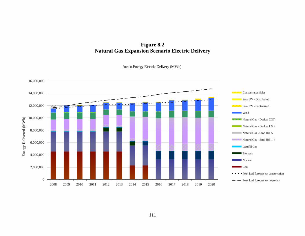
111

Figure 8.2

Natural Gas Expansion Scenario Electric Delivery


0

2,000,000

4,000,000

6,000,000

8,000,000

10,000,000

12,000,000

14,000,000

16,000,000

2008 2009 2010 2011 2012 2013 2014 2015 2016 2017 2018 2019 2020

Concentrated Solar



Wind





Landfill Gas

Biomass

Nuclear

Coal



En

erg

y D

eli

vere

d (

MW

h)

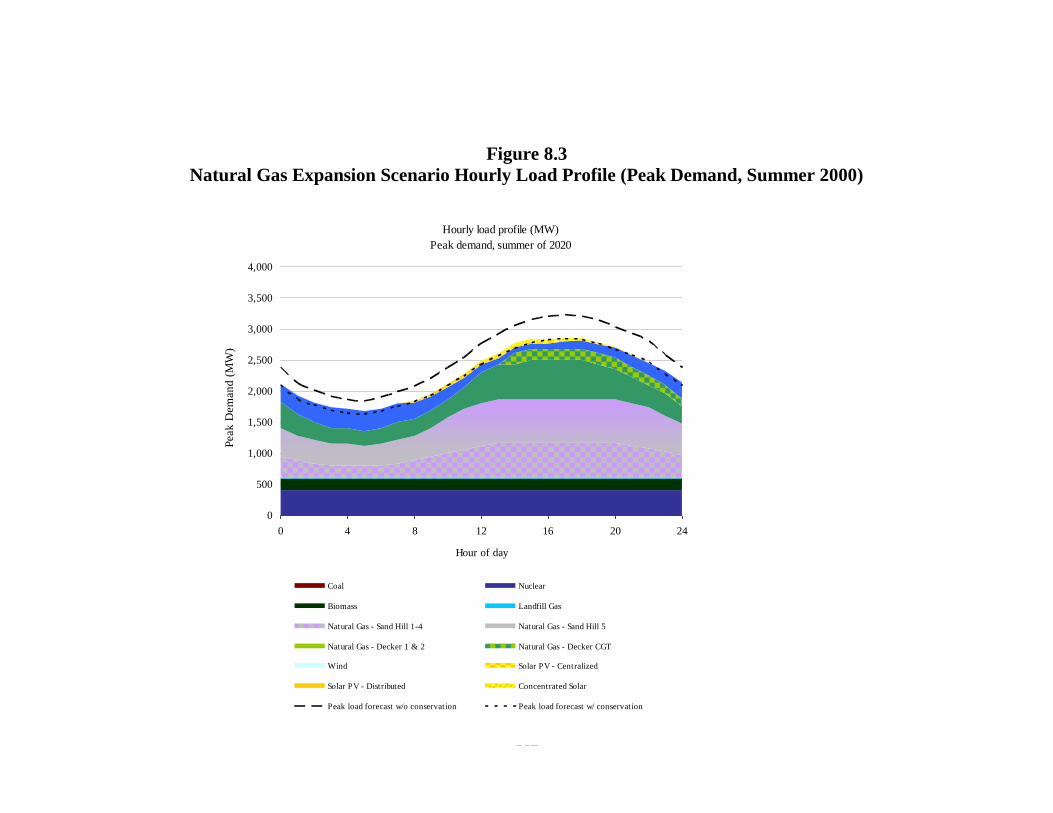
112

Figure 8.3

Natural Gas Expansion Scenario Hourly Load Profile (Peak Demand, Summer 2000)



0

500

1,000

1,500

2,000

2,500

3,000

3,500

4,000

0 4 8 12 16 20 24

Hour of day

Coal Nuclear







Peak

Dem

an

d (

MW

)

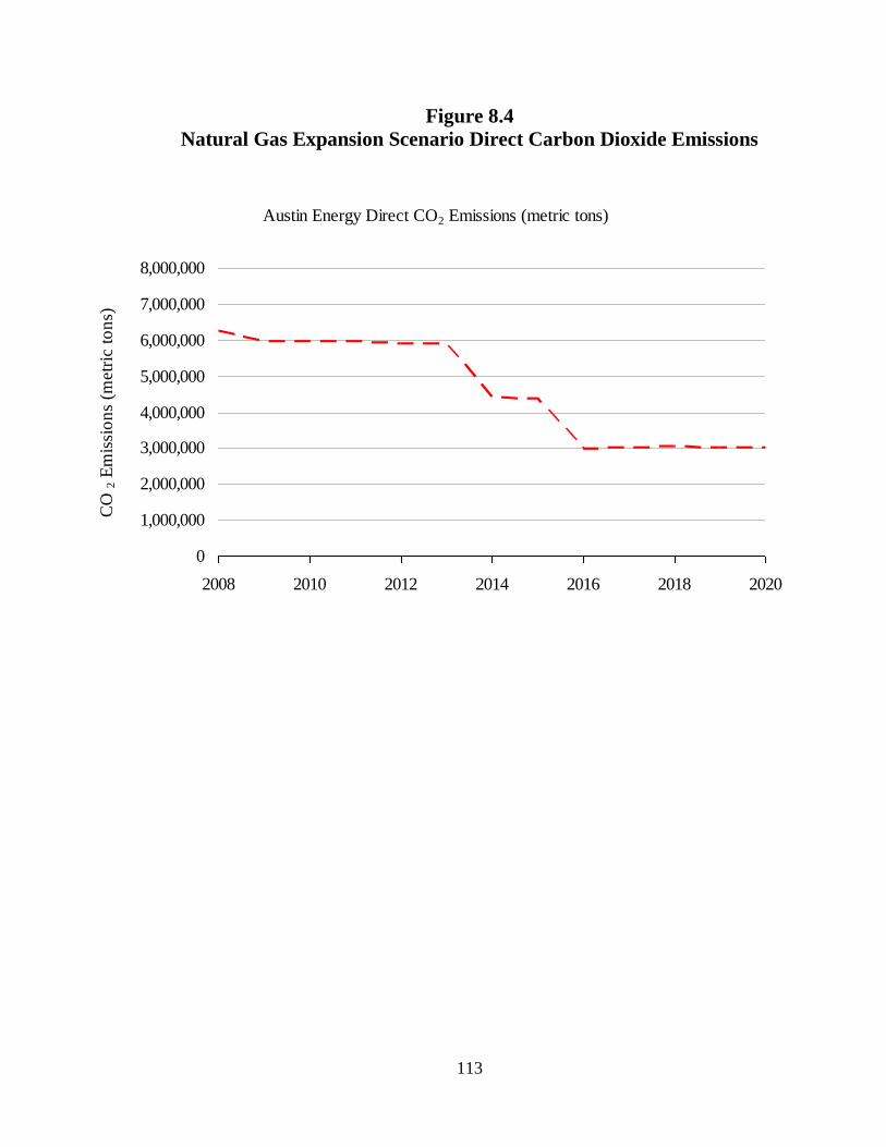
113

Figure 8.4

Natural Gas Expansion Scenario Direct Carbon Dioxide Emissions


0

1,000,000

2,000,000

3,000,000

4,000,000

5,000,000

6,000,000

7,000,000

8,000,000

2008 2010 2012 2014 2016 2018 2020

CO

2 E

mis

sio

ns

(metr

ic t

on

s)

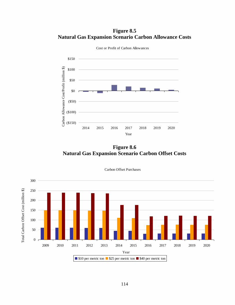
114

Figure 8.5

Natural Gas Expansion Scenario Carbon Allowance Costs

Figure 8.6

Natural Gas Expansion Scenario Carbon Offset Costs


($150)

($100)

($50)

$0

$50

$100

$150

2014 2015 2016 2017 2018 2019 2020

Year

Car

bon A

llow

ance

Co

st/P

rofi

t (m

illi

on $

)


0

50

100

150

200

250

300

2009 2010 2011 2012 2013 2014 2015 2016 2017 2018 2019 2020

Year


To

tal

Carb

on

Off

set

Co

st (

mil

lio

n $

)

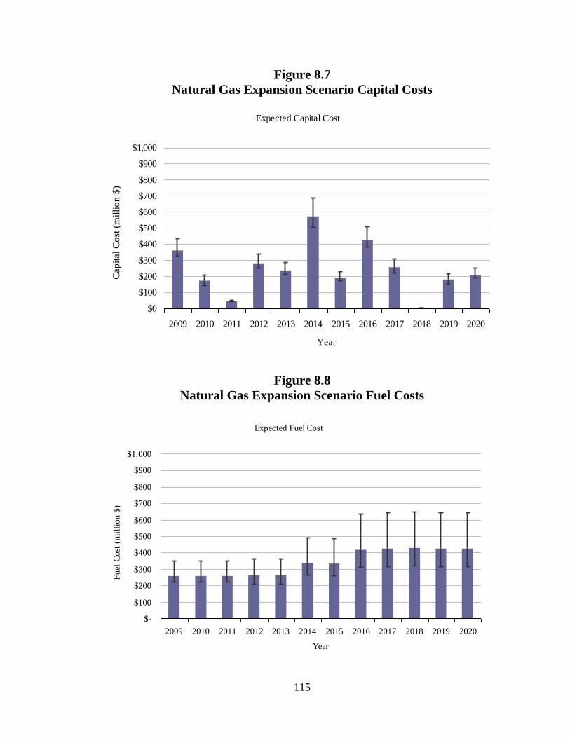
115

Figure 8.7

Natural Gas Expansion Scenario Capital Costs

Figure 8.8

Natural Gas Expansion Scenario Fuel Costs


$0

$100

$200

$300

$400

$500

$600

$700

$800

$900

$1,000

2009 2010 2011 2012 2013 2014 2015 2016 2017 2018 2019 2020

Year

Cap

ital

Co

st (

mil

lio

n $

)

Expected Fuel Cost

$-

$100

$200

$300

$400

$500

$600

$700

$800

$900

$1,000

2009 2010 2011 2012 2013 2014 2015 2016 2017 2018 2019 2020

Year

Fuel

Cost

(m

illi

on $

)

116

Figure 8.9

Natural Gas Expansion Scenario Levelized Costs


0

1

2

3

4

5

6

7

8

9

10

2009 2010 2011 2012 2013 2014 2015 2016 2017 2018 2019 2020

0%

10%

20%

30%

40%

50%

60%

70%

80%

90%




Wind





Landfill Gas

Biomass

Nuclear

Coal


Gen

era

tion

from

Cap

acity

Ad

ditio

ns (%

)

Ex

pecte

d I

ncre

ase

in

Lev

eli

zed

Ele

ctr

icit

y C

ost

(cen

ts/k

Wh

)

117

Figure 8.10

Natural Gas Expansion Scenario Economic Activity

Figure 8.11

Natural Gas Expansion Scenario Total Value Added

Figure 8.12

Natural Gas Expansion Employment Impacts

-$50,000,000

$0

$50,000,000

$100,000,000

$150,000,000

$200,000,000

$250,000,000

$300,000,000

$350,000,000

$400,000,000

$450,000,000

2006

2007

2008

2009

2010

2011

2012

2013

2014

2015

2016

2017

2018

2019

2020

Output (induced)

Output (indirect)

Output (direct)

-$50,000,000

$0

$50,000,000

$100,000,000

$150,000,000

$200,000,000

$250,000,000

$300,000,000

$350,000,000

2006

2007

2008

2009

2010

2011

2012

2013

2014

2015

2016

2017

2018

2019

2020




-500

0

500

1,000

1,500

2,000

2,500

3,000

3,500

2006

2007

2008

2009

2010

2011

2012

2013

2014

2015

2016

2017

2018

2019

2020



Employment (direct)

118

Chapter 9. Cleaner Coal Scenario

The cleaner coal scenario aligns with Austin Energy’s (AE) proposed energy resource

plan while replacing AE’s stake in FPP with a cleaner coal facility in 2020. This scenario

utilizes “clean coal” technologies to continue the use of coal in AE’s resource portfolio,

but reduces the amount of CO2 emissions into the atmosphere attributed to the burning of

coal. Under this scenario AE’s would divest its interest in the Fayette Power Project

(FPP) coal facility and replace the lose of power generated from this plant with coal-

based power generated by an Integrated Gasification Combined Cycle (IGCC) coal coal

plant with carbon capture and storage (CCS) technology. IGCC plants are more efficient

that traditional pulverized coals plants, but a large amount of energy is required to

operate the CCS process and it can be very costly to transport CO2 to an available storage

site. details additions to AE’s resource portfolio from 2009 to 2020 by fuel source,

power generation technology, or facility. IGCC plants have a capacity factor similar to

that of traditional coal fired power plants and nuclear power plants, so it can provide a

reliable source of baseload power. However, since an IGCC plant is designed to capture

energy losses and prevent deficiency below the desired output, capital costs come at

about a 45 percent increase over traditional coal plants.

Cleaner coal plants can provide a reliable source of energy as long as expenditure is

sufficient for CCS technology. Implementation of carbon regulation could make IGCC

plants with CCS technology much more cost competitive with traditional coal plants.

Coal power generation faces other risks. Coal mining and transport costs have increased

over the years and may continue to do so. Fifty coal plants have been cancelled or

postponed since January 2007, illustrating the increased risk and uncertainty perceived by

the public regarding coal-based power generation. Whether IGCC with CCS technology

can be operational at the scale necessary to replace FPP by 2020 is uncertain.

This scenario was run to show the sensitivity of using cleaner coal expansion in AE’s

resource portfolio. Cleaner coal technology presents a much more sustainable source of

power generation than fossil fueled technologies because they utilize coal resource that

are not depleted during the energy conversion process.

System Reliability

Replacing AE’s stake in the FPP with a cleaner coal facility does not create concerns

regarding system reliability because this new facility can still provide baseload power

generation (607 MW of power generation capacity.) Figure 9.1 demonstrates that AE’s

power generation capacity would exceed forecasted peak load with and without

conservation goals being met. This scenario would consist of 3,923 MW of power

generation capacity in 2020, the same amount of power generation capacity under AE’s

proposed energy resource plan.

Given the expected capacity factors for on-shore wind and solar PV (29 and 17 percent,

respectively) as well as current capacity factors for AE’s coal, nuclear, and natural gas

119

facilities AE will be able to deliver electricity reliably to its customers under this

scenario, given that AE meets its conservation goals (see Figure 9.2). Figure 9.3 details

AE’s expected hourly load profile for the hottest day (peak demand) in the summer of

2020. The hourly load profile demonstrates that AE will be able to meet peak demand

without purchasing power in 2020.


By reducing CO2 emissions caused by the burning of coal, CO2 emissions would drop

dramatically under this scenario (see Figure 9.4). AE’s CO2 emissions in 2007 were

roughly 6.1 million metric tons. Under this scenario CO2 emissions would drop to 1.8

million metric tons by 2020, a reduction of about 70 percent.

By reducing carbon emissions AE could profit if carbon regulation were to be passed that

supported a portion of allowances being given for free. Under the Lieberman-Warner

Climate Security Act of 2007, a portion of an entity’s emissions would be accounted for

by free permits, or allowances, while a portion of allowances would be auctioned. Figure

9.5 estimates that AE could make about $50 million in 2020 based upon allowance price

estimates for the Lieberman-Warner bill under this scenario.

Under this scenario, offsetting CO2 emissions to zero also becomes much more

manageable. Figure 9.6 provides a range of annual costs to offset emissions to zero, thus

achieving carbon-neutrality. The costs of offsets would be dramatically reduced in 2020,

when the transition to cleaner coal occurred. In 2020, annual carbon costs would decline

to $18 to $72 million annually compared to $58 to $230 million under AE’s proposed

resource plan.


Relative to oil or natural gas, coal is currently the least expensive fossil fuel used to

generate electric power. Cleaner coal technology facilitates use of coal while increasing

the efficiency of generating electricity and decreasing CO2 emissions. However, such

efficiency and environmental gains come at a high cost. Figure 9.7 details the capital cost

estimates for AE’s scheduled and proposed additions to its power generation mix. Total

expected capital costs under this scenario summed over the years 2009 to 2020 range

from $5.72 to $10.09 billion (compared to $2.2 to $3.01 billion under AE’s proposed

resource plan). Capital costs are expressed as total overnight costs. Therefore, it is

important to recognize the year for which a project is proposed.

Figure 9.8 details annual fuel costs for this scenario. As fossil-fueled sources do not

change dramatically under this scenario, fuel costs are expected to remain fairly stable,

ranging in any given year from $170 to $360 million which is almost the same as AE’s

resource plan. If carbon legislation or other fossil-fueled related regulation is

implemented over the next decade, fuel costs (primarily for coal and natural gas) would

likely move towards the high estimate.

120


impact of the levelized costs of new power generation resources, as a percentage of

overall power generation capacity. Under this scenario customers would expect the cost

of electricity to 4.5-7.3 cents per kilowatt-hour. It should be noted that this expected

increase in electric rates is based solely on new power generation investments. Offset

costs or any unexpected additional costs to the utility could also be passed on to the

customer during this time period. Additionally, the calculation for expected increase in

cost of electricity does not appoint a monetary value of reducing or removing coal or any

other resource from AE’s resource portfolio as the methods for evaluating how much AE

could receive are beyond the scope of this report. Such removal may help to alleviate the

additional costs to electricity accrued from the identified resource additions.

Figure 9.10 shows the economic output in the Greater Austin Area generated by the

cleaner coal scenario. Local economic activity peaks above $200 million in 2016. Figure

9.11 shows the total value added to the Greater Austin Area from the investments made

in the cleaner coal scenario. Figure 9.12 shows the impacts on employment created

through the cleaner coal scenario.

121

Table 9.1

Cleaner Coal Scenario Scheduled Additions and Subtractions to Generation Mix

2008 2009 2010 2011 2012 2013 2014 2015 2016 2017 2018 2019 2020

Coal 607 0 0 0 0 0 0 0 0 0 0 0 -607

Nuclear 422 0 0 0 0 0 0 0 0 0 0 0 0





Wind 274 165 0 23 0 0 50 100 0 74 0 50 110

Offshore Wind 0 0 0 0 0 0 0 0 0 0 0 0 0

Biomass 0 0 0 0 100 0 0 0 100 0 0 0 0


Landfill Gas 12 0 0 0 0 0 0 0 0 0 0 0 0




IGCC w/ CCS 0 0 0 0 0 0 0 0 0 0 0 0 607

IGCC w/o CCS 0 0 0 0 0 0 0 0 0 0 0 0 0

Geothermal 0 0 0 0 0 0 0 0 0 0 0 0 0

Storage 0 0 0 0 0 0 0 0 0 0 0 0 0


Purchased Power 0 0 0 0 0 0 0 0 0 0 0 0 0


122

Figure 9.1

Cleaner Coal Scenario Power Generation Capacity


0

500

1,000

1,500

2,000

2,500

3,000

3,500

4,000

2008 2009 2010 2011 2012 2013 2014 2015 2016 2017 2018 2019 2020

Concentrated Solar



Wind





Landfill Gas

IGCC w/ CCS

Biomass

Nuclear

Coal



Cap

acity

(M

W)

123

Figure 9.2

Cleaner Coal Scenario Electric Delivery


0

2,000,000

4,000,000

6,000,000

8,000,000

10,000,000

12,000,000

14,000,000

16,000,000

2008 2009 2010 2011 2012 2013 2014 2015 2016 2017 2018 2019 2020

Concentrated Solar



Wind





Landfill Gas

IGCC w/ CCS

Biomass

Nuclear

Coal



En

erg

y D

eli

vere

d (

MW

h)

124

Figure 9.3

Cleaner Coal Scenario Hourly Load Profile (Peak Demand, Summer 2000)



0

500

1,000

1,500

2,000

2,500

3,000

3,500

4,000

0 4 8 12 16 20 24

Hour of day

Coal FPP w/ biomass co-firing

Nuclear Biomass

IGCC w/ CCS Landfill Gas






Peak

Dem

an

d (

MW

)

125

Figure 9.4

Cleaner Coal Scenario Direct Carbon Dioxide Emissions


0

1,000,000

2,000,000

3,000,000

4,000,000

5,000,000

6,000,000

7,000,000

8,000,000

2008 2010 2012 2014 2016 2018 2020

CO

2 E

mis

sio

ns

(metr

ic t

on

s)

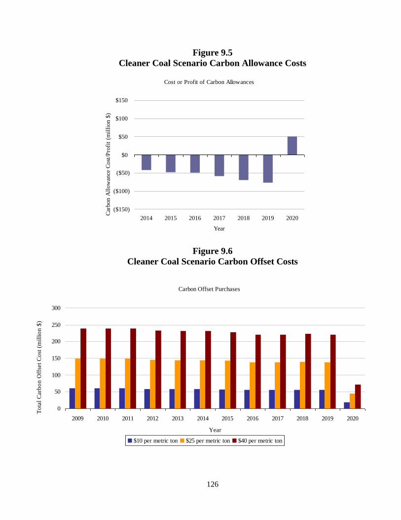
126

Figure 9.5

Cleaner Coal Scenario Carbon Allowance Costs

Figure 9.6

Cleaner Coal Scenario Carbon Offset Costs


($150)

($100)

($50)

$0

$50

$100

$150

2014 2015 2016 2017 2018 2019 2020

Year

Car

bon A

llow

ance

Co

st/P

rofi

t (m

illi

on $

)


0

50

100

150

200

250

300

2009 2010 2011 2012 2013 2014 2015 2016 2017 2018 2019 2020

Year


To

tal

Carb

on

Off

set

Co

st (

mil

lio

n $

)

127

Figure 9.7

Cleaner Coal Scenario Capital Costs

Figure 9.8

Cleaner Coal Scenario Fuel Costs


$0

$1,000

$2,000

$3,000

$4,000

$5,000

2009 2010 2011 2012 2013 2014 2015 2016 2017 2018 2019 2020

Year

Cap

ital

Co

st (

mil

lio

n $

)

Expected Fuel Cost

$-

$100

$200

$300

$400

$500

$600

$700

$800

$900

$1,000

2009 2010 2011 2012 2013 2014 2015 2016 2017 2018 2019 2020

Year

Fuel

Cost

(m

illi

on $

)

128

Figure 9.9

Cleaner Coal Scenario Levelized Costs


0

1

2

3

4

5

6

7

8

9

10

2009 2010 2011 2012 2013 2014 2015 2016 2017 2018 2019 2020

0%

10%

20%

30%

40%

50%

60%

70%

80%

90%




Wind





Landfill Gas

IGCC w/ CCS

Biomass

Nuclear

Coal


Gen

era

tion

from

Cap

acity

Ad

ditio

ns (%

)

Ex

pecte

d I

ncre

ase

in

Lev

eli

zed

Ele

ctr

icit

y C

ost

(cen

ts/k

Wh

)

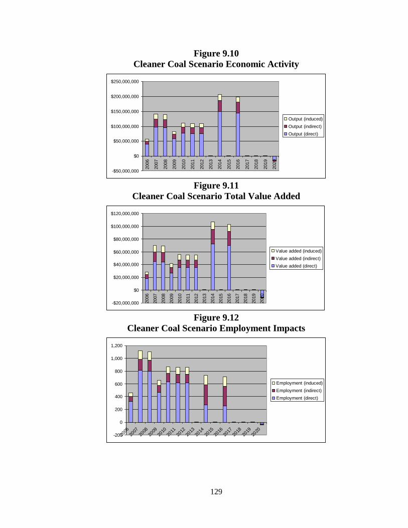
129

Figure 9.10

Cleaner Coal Scenario Economic Activity

Figure 9.11

Cleaner Coal Scenario Total Value Added

Figure 9.12

Cleaner Coal Scenario Employment Impacts

-$50,000,000

$0

$50,000,000

$100,000,000

$150,000,000

$200,000,000

$250,000,000

2006

2007

2008

2009

2010

2011

2012

2013

2014

2015

2016

2017

2018

2019

2020

Output (induced)

Output (indirect)

Output (direct)

-$20,000,000

$0

$20,000,000

$40,000,000

$60,000,000

$80,000,000

$100,000,000

$120,000,000

2006

2007

2008

2009

2010

2011

2012

2013

2014

2015

2016

2017

2018

2019

2020




-200

0

200

400

600

800

1,000

1,200

2006

2007

2008

2009

2010

2011

2012

2013

2014

2015

2016

2017

2018

2019

2020



Employment (direct)

130

Chapter 10. High Renewables Without Nuclear Scenario

The schedule for this scenario is identical to the schedule for the high renewables

scenario with three exceptions. Table 10.1 details the additions and subtractions made to

AE’s resource portfolio from 2009 to 2020 by fuel source, power generation technology,

or facility under this scenario. This scenario includes a slight acceleration in the addition

of geothermal capacity as well as a delay in divestment in coal. The more significant

change is the removal of 422 MW of nuclear power (the power generating capacity of the

South Texas Project, where AE generates its nuclear energy) from AE’s resource

portfolio. This divestment is scheduled for 2016 and represents the only net difference

between this scenario and the high renewables scenario. Therefore, this scenario holds the

same optimism with regards to the availability of renewable resources through 2020. One

difference between this scenario and the high renewable scenario (portfolio option 3) is

that with the loss of its stake in a coal and nuclear plant AE would no longer receive

energy from a baseload power source of significant capacity. Rather, AE would become

reliant upon technologies with variable availability.

System Reliability


peak load with and without conservation goals being met. The high renewables without

nuclear scenario includes 1,990 MW of wind and 913 MW of solar-based generation,

including two large-scale concentrated solar facilities using parabolic troughs and gradual

investment in distributed rooftop photovoltaic units. The mix of onshore and offshore

wind facilities is intended to exploit the complementary availabilities of both

technologies, given that onshore wind is most readily available in the evening and early

morning and offshore wind is most readily available during the day.



gas facilities, AE would be able to reliably deliver electricity for most days not occurring

in peak months.

The loss of nuclear as a reliable baseload source of power makes AE much more

vulnerable to gaps in variable resource availability and could necessitate a much greater

reliance on power purchased on the spot market. To demonstrate the risks of a system

highly dependent on wind and solar energy, Figure 10.3 details AE’s expected hourly

load profile for the hottest day (peak demand) in the summer of 2020. The hourly load

profile follows expected solar and wind profiles and demonstrates that AE will be able to

meet peak demand without purchasing power even on the hottest day of the summer, if

expected wind and solar production is met and AE meets its conservation goals. AE

would be unable to meet peak demand even if wind and solar energy meets expected

levels and natural gas facilities were operated at full capacity. This demonstrates great

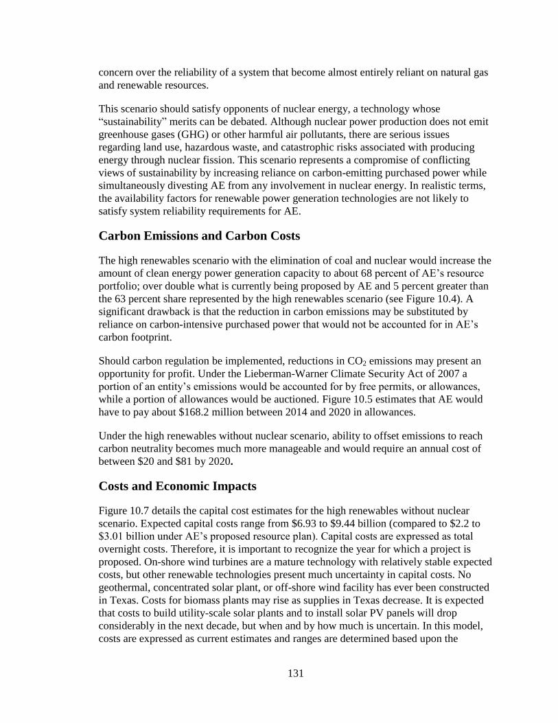
131

concern over the reliability of a system that become almost entirely reliant on natural gas

and renewable resources.

This scenario should satisfy opponents of nuclear energy, a technology whose

“sustainability” merits can be debated. Although nuclear power production does not emit

greenhouse gases (GHG) or other harmful air pollutants, there are serious issues

regarding land use, hazardous waste, and catastrophic risks associated with producing

energy through nuclear fission. This scenario represents a compromise of conflicting

views of sustainability by increasing reliance on carbon-emitting purchased power while

simultaneously divesting AE from any involvement in nuclear energy. In realistic terms,

the availability factors for renewable power generation technologies are not likely to

satisfy system reliability requirements for AE.


The high renewables scenario with the elimination of coal and nuclear would increase the

amount of clean energy power generation capacity to about 68 percent of AE’s resource

portfolio; over double what is currently being proposed by AE and 5 percent greater than

the 63 percent share represented by the high renewables scenario (see Figure 10.4). A

significant drawback is that the reduction in carbon emissions may be substituted by

reliance on carbon-intensive purchased power that would not be accounted for in AE’s

carbon footprint.

Should carbon regulation be implemented, reductions in CO2 emissions may present an

opportunity for profit. Under the Lieberman-Warner Climate Security Act of 2007 a

portion of an entity’s emissions would be accounted for by free permits, or allowances,

while a portion of allowances would be auctioned. Figure 10.5 estimates that AE would

have to pay about $168.2 million between 2014 and 2020 in allowances.

Under the high renewables without nuclear scenario, ability to offset emissions to reach

carbon neutrality becomes much more manageable and would require an annual cost of

between $20 and $81 by 2020.


Figure 10.7 details the capital cost estimates for the high renewables without nuclear

scenario. Expected capital costs range from $6.93 to $9.44 billion (compared to $2.2 to

$3.01 billion under AE’s proposed resource plan). Capital costs are expressed as total

overnight costs. Therefore, it is important to recognize the year for which a project is

proposed. On-shore wind turbines are a mature technology with relatively stable expected

costs, but other renewable technologies present much uncertainty in capital costs. No

geothermal, concentrated solar plant, or off-shore wind facility has ever been constructed

in Texas. Costs for biomass plants may rise as supplies in Texas decrease. It is expected

that costs to build utility-scale solar plants and to install solar PV panels will drop

considerably in the next decade, but when and by how much is uncertain. In this model,

costs are expressed as current estimates and ranges are determined based upon the

132

relative maturity of the technology and expected direction by which costs are expected to

flow.

Figure 10.8 details annual fuel costs under the high renewables without nuclear scenario.

Since the amount of fossil-fueled resources changes dramatically under this scenario, fuel

costs are expected to drop considerably, greatly reducing the risks associated with fuel

price instability. Fuel costs are expected to decrease gradually as coal usage is reduced

and eliminated. However, increased reliance on natural gas prevents fuel costs from

dropping significantly. By 2020 fuel costs under this scenario would range from $67 to

$172 million annually (compared to $93 to $328 million under AE’s proposed resource

plan).



generation capacity. The high renewables without nuclear scenario presents an almost

completely redefined power generation mix with almost 80 percent of actual power

generation coming from additions since 2009. Therefore, the costs of these additions will

have a significant impact on the costs of electricity. Since renewable power generation is

much more expensive than traditional fossil-fuel based power generation it is expected

that electric rates would rise considerably. It is estimated that this scenario would raise

the costs of electricity by 5 to 8 cents per kilowatt-hour. It should be noted that this

expected increase in electric rates is based solely on new power generation investments.

Offset costs or any unexpected additional costs to the utility could also be passed on to

the customer during this time period. Additionally, the calculation for expected increase

in cost of electricity does not appoint a monetary value of reducing or removing coal or

any other resource from AE’s resource portfolio as the methods for evaluating how much

AE could receive are beyond the scope of this report. Such removal may help to alleviate

the additional costs to electricity accrued from the identified resource additions.

Local economic development impacts could be significant under a high renewables

scenario depending upon the location of new power generation facilities. The most

significant impact upon the local economy would be created by the rapid acceleration in

solar PVs on rooftops. This could create a vibrant local solar manufacturing and

installation industry. Additionally centralized PV systems located within the Austin

region could further accelerate the solar industry in Austin.

The high renewable scenario represents a major increase in economic activity for the

Greater Austin Area attributed to investments in 250 MW of centralized photovoltaic

power generation facilities, 15 MW of landfill gas capacity, and 55 MW of distributed

photovoltaic power generation capacity. The most significant impact upon the local

economy would be created by the rapid acceleration in solar PV modules on rooftops.

This could create a vibrant local solar manufacturing and installation industry.

Additionally, centralized PV systems located within the Austin region could further

accelerate the solar industry in Austin. AE’s divestment in its stake in nuclear power

generated at the STP project would not directly affect the Greater Austin Area because

this plant is located several hundred miles away from Austin in Matagorda Bay.

133

Figure 10.10 shows the economic output in the Greater Austin Area generated by the

high renewables without nuclear scenario. Figure 10.11 shows the total value added to

the Greater Austin Area from the investments made in the high renewables without

nuclear scenario. Figure 10.12 shows the impacts on employment created through the

high renewables without nuclear scenario.

134

Table 10.1

High Renewables Without Nuclear Scenario Scheduled Additions and Subtractions to Generation Mix

2008 2009 2010 2011 2012 2013 2014 2015 2016 2017 2018 2019 2020

Coal 607 0 0 0 0 0 0 0 0 -302 0 0 -305

Nuclear 422 0 0 0 0 0 0 0 -422 0 0 0 0





Wind 274 165 0 100 0 0 100 200 0 526 0 100 220

Offshore Wind 0 0 0 0 50 0 50 0 50 0 50 0 105

Biomass 0 0 0 0 100 0 0 0 100 0 0 0 90


Landfill Gas 12 0 0 0 0 0 0 0 15 0 0 0 0




IGCC w/ CCS 0 0 0 0 0 0 0 0 0 0 0 0 0

IGCC w/o CCS 0 0 0 0 0 0 0 0 0 0 0 0 0

Geothermal 0 0 0 0 0 0 100 0 0 0 0 0 0

Storage 0 0 0 0 0 0 0 0 0 0 0 0 0


Purchased Power 0 0 0 0 0 0 0 0 0 0 0 0 0


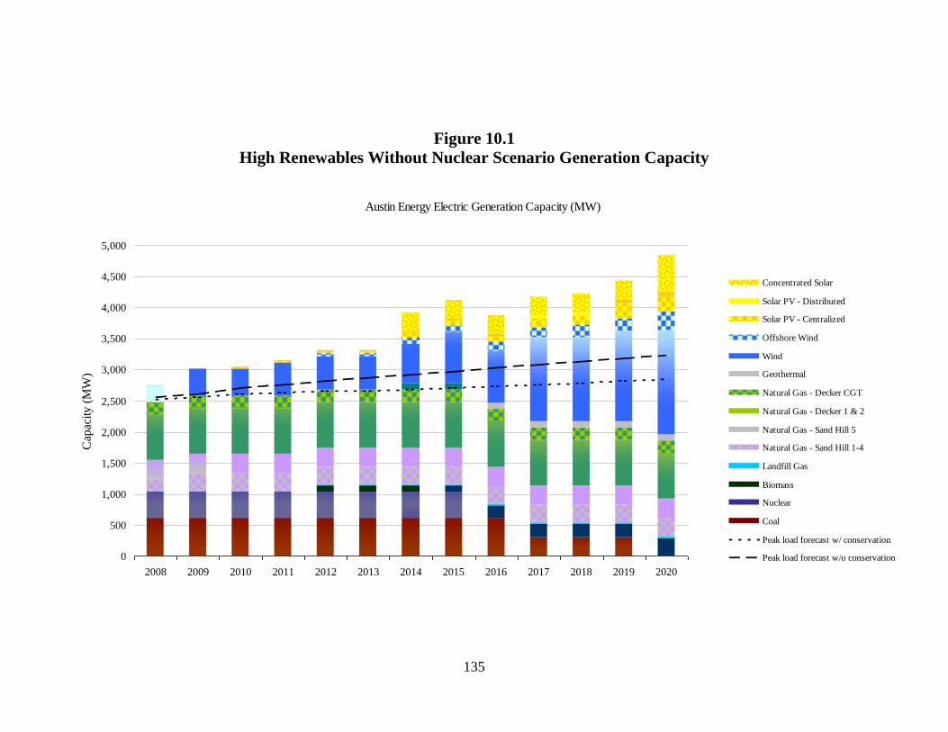
135

Figure 10.1

High Renewables Without Nuclear Scenario Generation Capacity


0

500

1,000

1,500

2,000

2,500

3,000

3,500

4,000

4,500

5,000

2008 2009 2010 2011 2012 2013 2014 2015 2016 2017 2018 2019 2020

Concentrated Solar



Offshore Wind

Wind

Geothermal





Landfill Gas

Biomass

Nuclear

Coal



Cap

acity

(M

W)

136

Figure 10.2

High Renewables Without Nuclear Scenario Electric Delivery


0

2,000,000

4,000,000

6,000,000

8,000,000

10,000,000

12,000,000

14,000,000

16,000,000

2008 2009 2010 2011 2012 2013 2014 2015 2016 2017 2018 2019 2020

Concentrated Solar



Offshore Wind

Wind

Geothermal





Landfill Gas

Biomass

Nuclear

Coal



En

erg

y D

eli

vere

d (

MW

h)

137

Figure 10.3

High Renewables Without Nuclear Scenario Hourly Load Profile (Peak Demand, Summer 2000)



0

500

1,000

1,500

2,000

2,500

3,000

3,500

4,000

0 4 8 12 16 20 24

Hour of day

Coal Nuclear




Geothermal Wind

Offshore Wind Solar PV - Centralized




Peak

Dem

an

d (

MW

)

138

Figure 10.4

High Renewables Without Nuclear Scenario Direct Carbon Dioxide

Emissions


0

1,000,000

2,000,000

3,000,000

4,000,000

5,000,000

6,000,000

7,000,000

8,000,000

2008 2010 2012 2014 2016 2018 2020

CO

2 E

mis

sio

ns

(metr

ic t

on

s)

139

Figure 10.5

High Renewables Without Nuclear Scenario Carbon Allowance Costs

Figure 10.6

High Renewables Without Nuclear Scenario Carbon Offset Costs


($150)

($100)

($50)

$0

$50

$100

$150

2014 2015 2016 2017 2018 2019 2020

Year

Car

bon A

llow

ance

Cost

/Pro

fit

(mil

lio

n $

)


0

50

100

150

200

250

300

2009 2010 2011 2012 2013 2014 2015 2016 2017 2018 2019 2020

Year


To

tal

Carb

on

Off

set

Co

st (

mil

lio

n $

)

140

Figure 10.7

High Renewables Without Nuclear Scenario Capital Costs

Figure 10.8

High Renewables Without Nuclear Scenario Fuel Costs


$0

$500

$1,000

$1,500

$2,000

$2,500

2009 2010 2011 2012 2013 2014 2015 2016 2017 2018 2019 2020

Year

Cap

ital

Co

st (

mil

lio

n $

)

Expected Fuel Cost

$-

$100

$200

$300

$400

$500

$600

$700

$800

$900

$1,000

2009 2010 2011 2012 2013 2014 2015 2016 2017 2018 2019 2020

Year

Fuel

Cost

(m

illi

on $

)

141

Figure 10.9

High Renewables Without Nuclear Scenario Levelized Costs


0

1

2

3

4

5

6

7

8

9

10

2009 2010 2011 2012 2013 2014 2015 2016 2017 2018 2019 2020

0%

10%

20%

30%

40%

50%

60%

70%

80%

90%




Offshore Wind

Wind

Geothermal





Landfill Gas

Biomass

Nuclear

Coal


Gen

era

tion

from

Cap

acity

Ad

ditio

ns (%

)

Ex

pecte

d I

ncre

ase

in

Lev

eli

zed

Ele

ctr

icit

y C

ost

(cen

ts/k

Wh

)

142

Figure 10.10

High Renewables Without Nuclear Scenario Economic Activity

Figure 10.11

High Renewables Without Nuclear Scenario Total Value Added

Figure 10.12

High Renewables Without Nuclear Scenario Employment Impacts

$0

$100,000,000

$200,000,000

$300,000,000

$400,000,000

$500,000,000

$600,000,000

2006

2007

2008

2009

2010

2011

2012

2013

2014

2015

2016

2017

2018

2019

2020

Output (induced)

Output (indirect)

Output (direct)

$0

$50,000,000

$100,000,000

$150,000,000

$200,000,000

$250,000,000

$300,000,000

2006

2007

2008

2009

2010

2011

2012

2013

2014

2015

2016

2017

2018

2019

2020




0

500

1,000

1,500

2,000

2,500

3,000

3,500

4,000

4,500

2006

2007

2008

2009

2010

2011

2012

2013

2014

2015

2016

2017

2018

2019

2020



Employment (direct)

143

Chapter 11. Accelerated Demand-Side Management

This chapter attempts to incorporate into the model scenarios some potential ranges of

demand reductions that Austin Energy (AE) could realistically achieve through

accelerated conservation strategies. Measured reductions in both peak power demand and

overall electricity demand due to utility-scale demand-side management (DSM), energy

efficiency, and pricing mechanisms have been surveyed and documented in Chapter 3 of

Volume II of this report. This chapter uses median values from those reports to obtain a

rough estimate of the potential impact of conservation strategies on the AE proposed

resource plan modeled scenario found in chapter 2 of this volume of the report. lists the

planned additions to AE’s resource portfolio from 2009 to 2020 by fuel source, power

generation technology, or facility and includes demand savings by year.

Utility-scale studies have reported a wide variety of potential energy savings that stem

from three basic strategies: energy efficiency, time-of-use pricing, and demand response

programs. Energy efficiency strategies would implement system-wide appliance and

equipment upgrades to lower overall energy demand. Time-of-use pricing and demand-

response programs would achieve reductions primarily in peak power demand. Rough-

estimate median values from the wide range of energy savings have been gathered to

generate new load profiles from the original AE load forecast through 2020. These load

profiles are provided as Figures 11.1-11.3. This chapter assumes that energy efficiency

measures could achieve annual energy demand reductions of 24 percent by 2020 [in

megawatt-hours (MWh)]. This chapter assumes that time-of-use pricing and demand-

response programs could achieve 22 percent peak demand savings (in MW) combined, or

approximately 10 percent savings in total energy demand (in MWh). The combination of

these strategies could theoretical achieve peak demand savings of 40 percent (in MW)

and overall demand savings of just over 30 percent (in MWh). In comparison, the

demand forecast in the AE proposed energy resource plan that includes conservation

efforts would reduce both peak demand and overall energy consumption by

approximately 12 percent. To implement these forecasts into the model, the values were

assumed to be implemented at a constant rate during each year, established by the end

savings percentage used divided by approximately 11 years.

System Reliability

Pursuing very aggressive energy efficiency and DSM measures could have a substantial

impact on AE’s future (see Figures 11.4-11.6). Drastically reducing overall demand

would allow AE to rely on fewer new power generation facilities. Demand reductions are

assumed to be achieved at all hours of the year so this mix gains reliability as it does not

have to rely heavily on variable power generation technologies (wind and solar) as much.

The demand reductions are so large that it is no longer necessary for AE to burn coal to

produce electricity by 2020. Nuclear and natural gas power sources could become the

primary producers of electricity. Natural gas would be used sparingly by 2020 and offer

more than enough back-up capacity for variable resources when needed.

144


The modeled aggressive conservation measure eliminates the need for the Fayette Power

Project coal plant by 2020. The demand reduction is so large in this scenario that carbon

emissions are reduced to the levels seen only in other very high renewables and carbon-

free scenarios. Figures 11.7-11.9 demonstrate the impacts of accelerated conservation on

carbon emissions and carbon costs.


DSM and efficiency strategies are generally among the cheapest ways to produce, or in

the case, negate the use of, energy. Figures 11.10 and 11.11 demonstrate the impact of

this scenario on yearly capital and fuel costs. The capital cost requirements to achieve all

these strategies are estimated to be $4.5-$6.1 billion through 2020 (compared to AE’s

proposed resource which is estimated to cost between $2.1 and 2.9 billion in capital).

Fuel costs are increased in this scenario in relation to AE’s proposed resource plan from

$130-270 million in 2020 to $155-$340 million, primarily due to an increased reliance on

natural gas facilities. Associated levelized cost of electricity values were unable to be

estimated in this analysis since DSM and efficiency strategies are not technically power

generation technologies.

145

Table 11.1

Accelerated DSM Scenario Scheduled Additions and Subtractions to Generation Mix

2008 2009 2010 2011 2012 2013 2014 2015 2016 2017 2018 2019 2020

Coal 607 0 0 0 0 0 0 0 -100 -100 -100 -200 -107

Nuclear 422 0 0 0 0 0 0 0 0 0 0 0 0





Wind 274 165 0 23 0 0 50 100 0 74 0 50 110

Offshore Wind 0 0 0 0 0 0 0 0 0 0 0 0 0

Biomass 0 0 0 0 100 0 0 0 100 0 0 0 0


Landfill Gas 12 0 0 0 0 0 0 0 0 0 0 0 0




IGCC w/ CCS 0 0 0 0 0 0 0 0 0 0 0 0 0

IGCC w/o CCS 0 0 0 0 0 0 0 0 0 0 0 0 0

Geothermal 0 0 0 0 0 0 0 0 0 0 0 0 0

Storage 0 0 0 0 0 0 0 0 0 0 0 0 0


Purchased Power 0 0 0 0 0 0 0 0 0 0 0 0 0


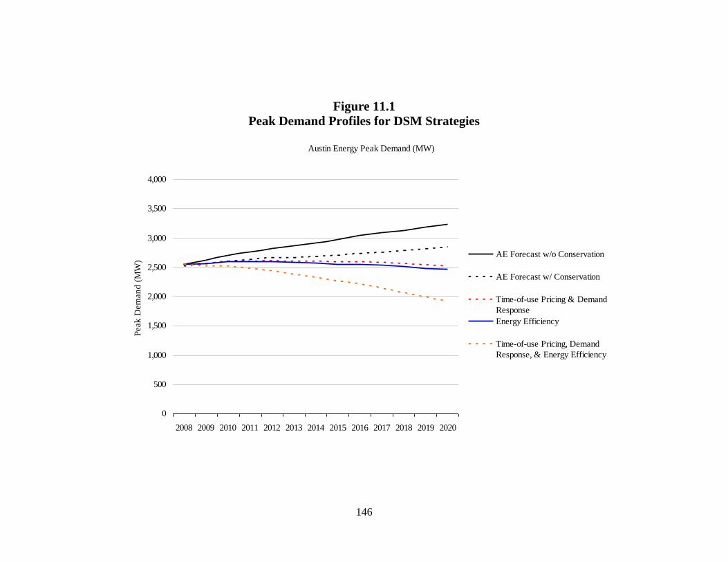
146

Figure 11.1

Peak Demand Profiles for DSM Strategies

Austin Energy Peak Demand (MW)

0

500

1,000

1,500

2,000

2,500

3,000

3,500

4,000

2008 2009 2010 2011 2012 2013 2014 2015 2016 2017 2018 2019 2020

AE Forecast w/o Conservation

AE Forecast w/ Conservation

Time-of-use Pricing & Demand

Response

Energy Efficiency

Time-of-use Pricing, Demand

Response, & Energy Efficiency

Peak

Dem

an

d (

MW

)

147

Figure 11.2

Annual Electricity Demand Profiles for DSM Strategies

Austin Energy Annual Electric Demand (MWh)

0

2,000,000

4,000,000

6,000,000

8,000,000

10,000,000

12,000,000

14,000,000

16,000,000

2008 2009 2010 2011 2012 2013 2014 2015 2016 2017 2018 2019 2020



Time-of-use Pricing & Demand

Response

Energy Efficiency

Time-of-use Pricing, Demand

Response, & Energy Efficiency

An

nu

al

Dem

an

d (

MW

h)

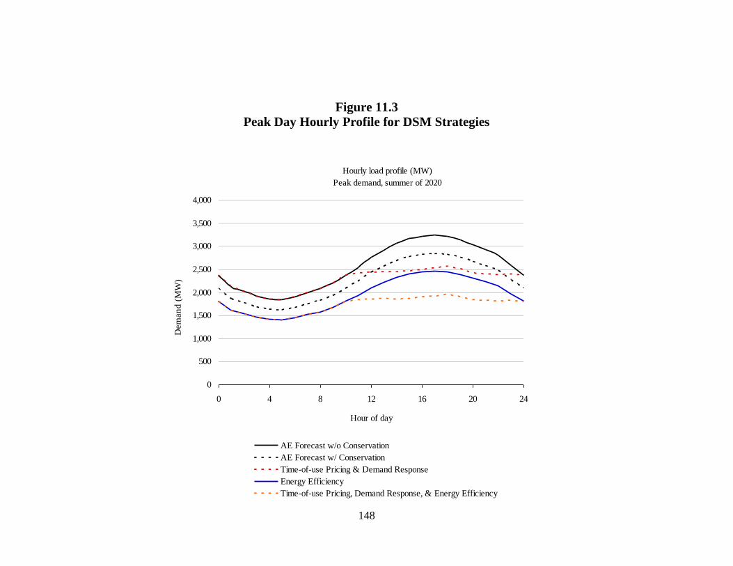
148

Figure 11.3

Peak Day Hourly Profile for DSM Strategies



0

500

1,000

1,500

2,000

2,500

3,000

3,500

4,000

0 4 8 12 16 20 24

Hour of day



Time-of-use Pricing & Demand Response

Energy Efficiency

Time-of-use Pricing, Demand Response, & Energy Efficiency

Dem

an

d (

MW

)

149

Figure 11.4

Accelerated DSM Scenario Power Generation Capacity


0

500

1,000

1,500

2,000

2,500

3,000

3,500

4,000

2008 2009 2010 2011 2012 2013 2014 2015 2016 2017 2018 2019 2020

Concentrated Solar



Wind





Landfill Gas

Biomass

Nuclear

Coal

Peak load forecast w/ DSM Strategies


Cap

acity (

MW

)

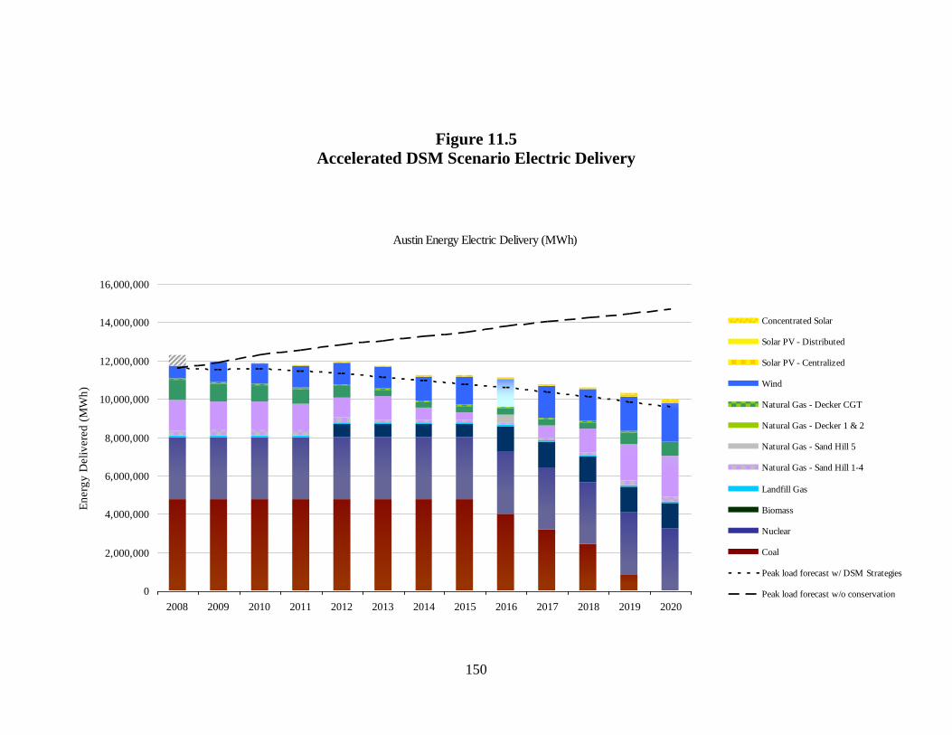
150

Figure 11.5

Accelerated DSM Scenario Electric Delivery


0

2,000,000

4,000,000

6,000,000

8,000,000

10,000,000

12,000,000

14,000,000

16,000,000

2008 2009 2010 2011 2012 2013 2014 2015 2016 2017 2018 2019 2020

Concentrated Solar



Wind





Landfill Gas

Biomass

Nuclear

Coal



En

erg

y D

eli

vere

d (

MW

h)

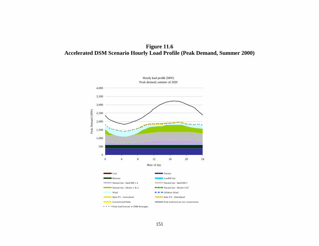
151

Figure 11.6

Accelerated DSM Scenario Hourly Load Profile (Peak Demand, Summer 2000)



0

500

1,000

1,500

2,000

2,500

3,000

3,500

4,000

0 4 8 12 16 20 24

Hour of day

Coal Nuclear




Wind Offshore Wind

Solar PV - Centralized Solar PV - Distributed

Concentrated Solar Peak load forecast w/o conservation


Pea

k D

eman

d (

MW

)

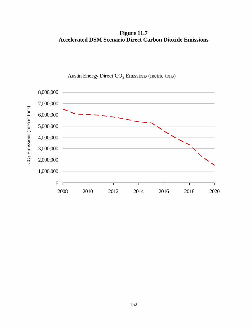
152

Figure 11.7

Accelerated DSM Scenario Direct Carbon Dioxide Emissions


0

1,000,000

2,000,000

3,000,000

4,000,000

5,000,000

6,000,000

7,000,000

8,000,000

2008 2010 2012 2014 2016 2018 2020

CO

2 E

mis

sio

ns

(met

ric

ton

s)

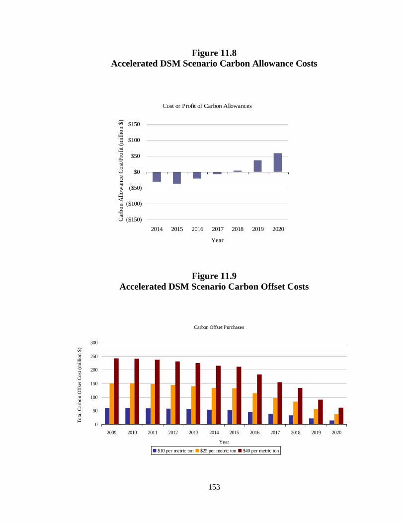
153

Figure 11.8

Accelerated DSM Scenario Carbon Allowance Costs

Figure 11.9

Accelerated DSM Scenario Carbon Offset Costs


($150)

($100)

($50)

$0

$50

$100

$150

2014 2015 2016 2017 2018 2019 2020

Year

Car

bo

n A

llo

wan

ce C

ost

/Pro

fit

(mil

lio

n $

)


0

50

100

150

200

250

300

2009 2010 2011 2012 2013 2014 2015 2016 2017 2018 2019 2020

Year


To

tal

Carb

on

Off

set

Co

st (

mil

lio

n $

)

154

Figure 11.10

Accelerated DSM Scenario Capital Costs

Figure 11.11

Accelerated DSM Scenario Fuel Costs


$0

$100

$200

$300

$400

$500

$600

$700

$800

$900

$1,000

2009 2010 2011 2012 2013 2014 2015 2016 2017 2018 2019 2020

Year

Cap

ital

Co

st (

mil

lio

n $

)

Expected Fuel Cost

$-

$100

$200

$300

$400

$500

$600

$700

$800

$900

$1,000

2009 2010 2011 2012 2013 2014 2015 2016 2017 2018 2019 2020

Year

Fuel

Cost

(m

illi

on $

)

155

Chapter 12. Conclusions and Recommendations

The evaluation model developed by the project team allows one to compare different

investment options that would reshape Austin Energy’s (AE) resource portfolio by 2020.

Seven primary scenarios that demonstrate the diversity of investment opportunities

identified by the project team in Volume II of this report were run for comparison with

AE’s proposed energy resource plan. Additionally, the impact of demand-side

management (DSM) savings exceeding AE’s goal of 700 megawatts (MW) of demand

savings by 2020 is also included in this report. The seven primary scenarios evaluated

include: nuclear expansion; high renewable energy investment; expected available

renewable energy investment; expected available renewable energy investment with

energy storage capacity; natural gas expansion; coal with carbon capture and

sequestration facility to replace current coal facility; and high renewable energy

investment to replace both coal and nuclear. Included with several of the primary

scenario analyses is an appendix that details the impact of each major resource or

technology investment within each individual primary scenario. The appendices are

intended to serve as a sensitivity analysis of each resource or technology investment

made in a given scenario or other degrees of investment that could be made in a particular

resource or technology. Table 12.1 lists the energy resource mix scenarios evaluated and

the components of the analysis of these scenarios. The scenarios evaluated and their

associated outputs are not intended to provide a complete list of all of the possible

investments that could be made by AE through 2020. Rather, the intention is to evaluate a

diverse range of options with a model that has the ability to easily evaluate new options

as they are presented.

In this chapter, resource portfolio scenarios are compared using measures that indicate

four criteria: system reliability, carbon reductions, costs and economic impacts, and risks

and uncertainties. This report is intended to inform AE customers and the general public

about the impact that investments in different energy resources and power generation

technologies may have upon these criteria. Comparative tables with rankings based on

measures identified for each of the four factors are provided in this chapter.

The primary goal of this report is to evaluate sustainable energy options for AE with the

interim goal of reaching carbon neutrality by 2020. Therefore, we believe that the impact

of different investments on AE’s carbon footprint should have the greatest significance

for the findings and recommendations provided herein. While all of the primary scenarios

demonstrate reductions in AE’s carbon footprint, the amount of reduction varies

considerably in degree and cost. A comparative table that ranks the eight scenarios in

terms of costs of carbon reductions is included in this chapter.

Comparison of Resource Portfolios

The goal of the model is to provide a simple tool for comparing different energy resource

portfolios. The model created for the purposes of this evaluation has the capacity to be

156

quickly and easily run for any investment plan identified by a user (albeit limited by the

models inputs). Eight scenarios have been evaluated for comparison of their impacts

upon AE’s power system. In Chapters 2 through 9 of this volume of the report, the actual

outputs generated by the model for each scenario are accompanied by an interpretation

and analysis of each scenario. These eight scenarios are not intended to preclude the

consideration or evaluation of other potential investment plans.

These eight scenarios have been identified to recognize and assess the impacts of

different approaches to reducing AE’s carbon footprint. These scenarios provide a diverse

set of options by focusing on different types of energy resources and power generation or

energy storage technologies. The intent of the comparison of these eight scenarios is to

provide the reader of this report with an overview of a range of investment and

divestment opportunities along with information on the impact of these investments.

Almost every power generation or energy storage technology that has been identified by

the project team as a feasible investment opportunity between 2009 and 2020 is included

in one or more scenario. Each reader can consider the estimated consequences of

investing in her or his preferred technologies. Each user can use the raw data to design an

AE resource portfolio that she or he prefers.

The project team accepts that there is no easy way to compare these eight scenarios or

others that could or should be developed to explore AE’s diverse potential energy

portfolios. The project’s approach is to compare alternate scenarios based on four criteria:

system reliability, costs and economic impacts, CO2 emissions, and risks and

uncertainties. The tradeoffs among criteria are clear (as discussed below), so it is

important to construct a transparent comparison process as other analysts may wish to use

different metrics of comparison. It is possible for AE to reach close to carbon neutrality

by 2020 using any of the eight scenarios by using different approaches. The following

paragraphs compare the logic involved in these tradeoffs.

In some scenarios (high renewables) AE will spend a lot of money buying new renewable

energy sources in order to relieve current carbon-intensive fuels from service. Such

options may be more “sustainable” in the sense that renewable resources are carbon

neutral. If the US were to develop federal carbon regulations AE may be able to earn

returns on these investments in the form of allowances. Fuel costs would drop, so the

savings in fuel would eventually balance out the increased capital expenses. No

returnable private business discount rate is likely to justify the disproportionate

investment required to achieve the high renewables scenario, as the substantial annual

fuel savings would require many years to compensate AE for the capital investments.

The nuclear expansion option that allows for the retirement of coal-fueled electricity is a

different value judgment. Nuclear expansion can yield low-cost power and a zero carbon

footprint with the potential for carbon offset payments to morph into carbon allowances

that earn money for AE. The issue is whether the public is willing to accept the risks

associated with nuclear energy. Risks include very high capital costs, construction delays,

and political consideration of issues relating to the sustainable merits of nuclear energy

due to the production of radioactive wastes. As no new nuclear power plant has been built

157

in the US for several decades it is hard to assess whether estimated capital costs will fall

within “expected” values or be even more expensive per kWh than solar power. The

tradeoff is unintended risks versus expected costs, a value judgment that only elected

officials have the right to make.

The third example of tradeoffs among scenarios comes from AE’s base case, its resource

plan, where carbon neutrality could only be reached through an annual payment of carbon

offsets. One must judge whether the purchase of carbon offsets to achieve carbon

neutrality truly constitutes a sustainable electric utility. While AE’s resource plan has the

lowest incremental capital costs per kWh of the eight scenarios it also makes the least

progress towards carbon neutrality as it accepts the existing coal source and actually

expands reliance on natural gas as a complement to variable solar and wind resources.

The problem with this conceptual comparison among these scenarios (which could be

expanded to all eight scenarios or even other scenarios) is that is not easy to analyze such

marginal changes without making a value judgment. As a result, the project team has

attempted to evaluate the scenarios by identifying performance measures of interest to

AE’s customers. These measurements relate to certain criteria that impact investment

decisions in the electric utility industry. Table 12.2 lists the criteria used to evaluate the

eight primary scenarios identified by this report. For each criterion multiple

measurements are used to compute an ordinal ranking of the eight resource portfolio

scenarios under each criterion.

System Reliability

The primary goal of an electric utility provider is to provide reliable service by ensuring

that electricity is available at all times to meet customer demands. Measurements of

system reliability capture the ability of the utility to generate electricity to meet yearly

and peak demand, transmit and distribute electricity, and handle unexpected weather

events or technological failures. Total nameplate power generation capacity determines

the system’s entire capacity for generating power, but the size of the system can be

deceiving in terms of ability to generate electricity when a large proportion of the

capacity is attributed to variable power sources (e.g., wind and solar). Since wind and

solar cannot be relied upon to generate electricity at all times, we define the total

nameplate power generation capacity of all non-variable resources as a metric of

reliability. Utilities focus on peak demand to determine if their resource portfolio can

handle the highest level of demand expected. We define another reliability metric as the

ability of a resource portfolio to meet expected peak demand in 2020 as a fraction of peak

hourly demand met in 2020. Wind and solar hourly profiles are used to account for the

expected amount of electricity generated by these resources on a peak demand day. As

AE increases its reliance on variable resources it is important to recognize the risks and

uncertainties this poses to system reliability. Power generation attributed to wind and

solar is vulnerable to unavailability due to uncontrollable factors. Wind and solar power

generation is constrained by the magnitude of wind velocity and solar radiation on a

particular day at a particular time. One way to ensure reliable service from variable

energy sources is by “backing up” these sources with natural gas facilities that can be

158

quickly ramped up in case of expected or unexpected weather events or technological

failures. The ratio of available natural gas capacity over the course of the year (after

expected natural gas capacity is used) to solar and wind capacity provides an indication

of the ability of AE to provide electricity when necessary to account for lower than

expected variable resource power production. Reliance on natural gas is also measured to

indicate the availability of natural gas resources as a backup to variable resources. The

ability of AE to provide reliable electric service to its customers is not only determined

by its ability to produce power. AE must also have adequate transmission and distribution

infrastructure in place to ensure electricity can be transferred from its source to its end-

use. Since it is expected that most utility-scale renewable power generation plants will be

built in rural, scarcely populated regions of Texas, the percentage of power generation

attributed to biomass, geothermal, solar, and wind is measured as an indicator of the

transmission and distribution requirements necessary for a particular resource portfolio. It

is assumed that coal, natural gas, and nuclear facilities would be built in areas of the state

with existing adequate transmission and distribution infrastructure.

Table 12.3 summarizes the quantitative and qualitative system reliability indicators.

Based upon the measurements used in this analysis, AE’s energy resource plan emerges

as the leading candidate for ensuring system reliability. Only three of the scenarios are

able to meet peak demand without purchasing power from the electric grid: AE’s energy

resource plan, the high renewables scenario, and the expected available renewables with

energy storage scenario. The nuclear expansion scenario comes close to being able to

meet peak demand by doubling current nuclear capacity (from 422 MW to 844 MW) to

replace the 607 MW of power generation capacity attributed to coal. If AE were to

substitute all of the current coal power generation supply with nuclear (a 607 MW

addition of nuclear power generation capacity), it would be able to meet peak demand in

2020 and would ensure system reliability similarly to AE’s proposed resource plan. None

of the scenarios falls dramatically short of meeting peak demand. The two high

renewable scenarios appear to be the only two scenarios that face serious risks due to

reliance on unreliable variable energy resources, wind and solar. Under the high

renewables scenario, it appears that even if all of the expected wind and solar resources

were unavailable, 50 percent of the nameplate capacity would be supported by available

natural gas capacity. Since wind and solar capacity factors are already low, natural gas

capacity may be able to account for the complete loss of wind and solar availability even

under the high renewable scenario. The high renewables scenarios could only occur if

Texas’ proposed new transmission infrastructure is built. Texas is currently investing 5

billion dollar to build extensive transmission lines in West Texas to deliver electricity

from wind farms to the most populous cities in Texas. It is unclear whether these

investments would be able to transmit such a large investment in West Texas wind and

solar resources to AE. The feasibility of the high renewables case could depend on the

amount of investment by other utilities in wind and solar resources.

Carbon Emission Reductions

The primary purpose of this report is to identify investments that will help AE design a

sustainable electric utility that is carbon-neutral by 2020. Carbon-neutrality has been

159

defined by this report as eliminating AE’s carbon footprint by reducing direct carbon

dioxide (CO2) emissions as low as possible and offsetting the remaining emissions to

zero. Direct CO2 emissions are measured to demonstrate the ability of different

investments to reduce emissions from current levels prior to buying offsets. The expected

annual cost of offsetting the remaining emissions is provided as a separate measurement.

The expected annual cost or profit from buying or selling allowances under a carbon

regulatory framework is also measured.

Table 12.4 summarizes the quantitative and qualitative indicators of CO2 emissions and

associated potential carbon costs. Three outputs are generated related to CO2 emissions

and associated costs for three of the portfolio options (AE’s plan, nuclear expansion, and

high renewable): direct CO2 emissions by year through 2020 and expected costs or profits

from carbon allowances (based upon the proposed Lieberman-Warner Climate Security

Act of 2007). The three measurements are related, as the greater the reduction in CO2 the

lower the annual costs of offsets and allowances. The high renewable scenario achieves

annual CO2 reductions of over 5.5 million metric tons of CO2 by 2020 from 2007 levels

(about 6.1 million metric tons), the greatest reduction of all eight scenarios by at about 1

million metric tons. The nuclear expansion scenario achieves the second largest reduction

in CO2 emissions by 2020 and the AE resource plan achieves the lowest reduction in CO2

emissions, reducing between 2007 and 2020 annual emissions by about 300,000 metric

tons prior to the purchase of offsets. Under the high renewable scenario, it is estimated

that the annual costs of offsetting emissions would be about $14 million by 2020 at an

offset cost of $25 per metric ton of CO2 emitted. The cost of offsetting emissions in the

future is unclear due to the uncertainty of carbon regulation in the US. The cost of

offsetting emissions is fairly low currently (at about $4-8 a metric ton of CO2), but would

likely rise if carbon regulation is implemented in the US. Under the AE resource plan,

this cost would be about $144 million annually. Based upon the carbon regulatory

scheme proposed by the Lieberman-Warner bill, three of the scenarios would result in the

need for AE to purchase allowances in 2020: the AE resource plan (at an annual cost of

about $96 million); the expected available renewables scenario (at an annual cost of

about $31 million); and the natural gas expansion scenario (at an annual cost of about $31

million). The high renewable scenario would generate about $94 million annually

through the sale of allowances by 2020. The nuclear expansion scenario would generate

about $55 million annually through the sale of allowances. It is expected that the value of

allowances would continue to increase each year after 2020.


This report indicates that making investments with the intent of reducing AE’s carbon

footprint can entail significant costs, so the costs and expected impacts on customer

electric rates are another criteria posited by this analysis. To evaluate the total economic

impacts of a resource portfolio, various cost indicators are measured along with the

projected economic development impacts in Austin and surrounding counties. Total

expected capital costs measures the expected capital outlay (measured as total overnight

costs) that would be necessary through 2020 for a particular investment plan. Such costs

can affect electric rates, AE’s credit rating, and AE’s ability to finance new projects.

160

Total expected fuel costs measures the reliance on fossil fuels and the risk of volatile fuel

prices. Fuel costs may become increasingly volatile as competition for fossil fuels

increases with global economic activity. Carbon regulation could also affect fuel prices,

as combustion of fuels emits large amounts of CO2. The expected increase in levelized

cost of electricity attempts to capture the actual impact of investments on customer

electric bills. It should be noted that throughout this analysis no “value” is imputed to the

leasing or selling of AE’s share of ownership in a power plant facility in the levelized

cost of electricity. The calculators do not attempt to represent the flows of debts. Any sale

or lease of AE’s power plant ownership, such as its stake in FPP, could be used to pay for

the purchase of other power sources or could contribute to a reduction in electric rates at

that time.

Table 12.5 summarizes the quantitative and qualitative indicators of costs and economic

impacts. The expected capital costs of the high renewable scenarios (about $8.3 million)

exceed that of AE’s resource plan (about $2.2 million) by a factor of almost four. While

total expected fuel costs are about $600,000 lower in the high renewable scenario, lower

fuel costs do not offset the capital costs incurred during this time period. Selling or

leasing ownership in FPP would offset some of these costs under the high renewable

scenario. The natural gas expansion scenario would entail the lowest expected capital

costs (at about $1.4 million), but would have the greatest expected total fuel costs (at

about $4.8 million). Annual fuel costs by 2020 would be the highest under a natural gas

expansion scenario. The high renewables scenario would have the lowest annual expected

fuel costs by 2020, but it would take several decades for annual fuel costs, at current

prices, to offset the high capital costs. The expected increase in levelized costs of

electricity attempts to account for the costs of financing power generation projects and all

costs that go into the production of electricity including capital and variable costs. The

current cost of electricity for AE customers is about 10 cents per kWh, but varies based

upon the amount of electricity consumed during a billing period. The expected increase in

the cost of electricity is about 2 cents per kWh under AE’s proposed energy resource

plan. The expected renewables scenario would face an expected increase in cost of

electricity of 2.2 cents per kWh, but this does not capture the increased reliance on

natural gas that could raise the fuel charge for customers. The high renewable scenario

estimates an expected increase in the cost of electricity of about 5.8 cents per kWh by

2020. The cleaner coal scenario also demonstrates a high expected increase in cost of

electricity of 5.7 cents per kWh. The natural gas scenario estimates an expected increase

of 5.7 cents per kWh, but this may be misleading because much of the natural gas

expansion comes in the form of combustion turbines that would be used to provide large

amount of electricity. As it is unlikely that AE would operate combustion gas turbines at

high levels of use, actual costs would likely be lower with the expansion of combined

cycle facilities replacing combustion gas turbine expansion to be used for high levels of

use. The nuclear expansion scenario provides a middle ground cost of electricity increase

between AE’s resource plan and the high renewable scenario with an expected increase

of 3.9 cents per kWh. However, nuclear investments entail high capital cost risks and the

potential for project delays that could push costs higher. The AE resource plan appears to

be the least cost option followed by the expected renewable scenario and the nuclear

expansion scenario. The value of the sale or lease of FPP could alter this ranking.

161

Risks and Uncertainties

Any future is full of uncertainties, starting with the question of whether 2020 electricity

demand will be lower or relatively similar than demand in 2008 due to a prolonged

depression or whether growth will push 2020 demand at or above AE forecasts. Any

portfolio of power sources has risks and uncertainties associated with it. Measurements of

risks include uncertain cost estimates and reliance on variable resources or immature

technologies. High estimates of capital costs, fuel costs, and increases in levelized cost of

electricity represent one criterion of AE cost risks. The fraction of total demand met by

energy sources that vary (solar and wind) is an indicator of the risk of relying heavily on

sources of energy that are dependent on weather and wind patterns as well as time of day.

Reliance on new emerging technologies is another type of risks that will affect electricity

availability and reliability.

Table 12.6 lists indicators of risks and uncertainties. Taking the high estimate of total

capital costs, fuel costs, and increase in levelized cost of electricity does not alter the

ordinal rankings of these scenarios from expected costs. For example, the nuclear

expansion scenario faces the greatest capital costs and levelized cost of electricity risks

due to the uncertainty of the costs that will be incurred to build the nuclear expansion.

The natural gas expansion scenario faces the greatest fuel costs risk. The cleaner coal and

natural gas expansion scenarios have the lowest fraction of total demand met with

variable resources in 2020. The high renewables scenario places a considerable amount

of dependency on variable resources at almost 60 percent of electricity generated

(compared to 17 percent under AE’s resource plan). No other scenario places more than

24 percent reliance on variable resources in 2020. Risks from immature technologies are

greatest under the clean coal scenario, expected renewable with energy storage and the

high renewable scenarios.

Table 12.7 ranks the eight resource portfolio options by assigning equal weight to all

comparative measures within each criteria and then assigning equal weight to each

criteria to compute an average order ranking across the four criteria. While such a

measure which has no absolute meaning whatsoever, as it is an index of indices added

together, it is a means to compare scenarios. Of all the ways that multiple criteria can be

aggregated, this approach is used because it is transparent and simple; other users can

adopt their own multi-criteria measures.

The AE proposed energy resource plan receives the highest overall ranking despite

achieving the lowest reductions in CO2 because it received the highest ranking for system

reliability, costs and economic impacts, and risks and uncertainties. The nuclear

expansion scenario is ranked second because of the significant reductions the scenario

makes in CO2 emissions. The high renewable scenario receives a slightly higher ranking

than the expected available renewables, natural gas expansion, cleaner coal, and expected

available renewable with energy storage scenarios. The high renewables without coal and

nuclear scenario has by far the lowest average ranking of the eight scenarios. It appears

that the nuclear expansion scenario and AE’s resource plan receive comparable rankings

when the factors of system reliability, CO2 reductions, costs and economic impacts, and

162

risks and uncertainties are all assigned equal weight. AE’s resource plan is less costly,

more reliable, and faces lower risks and uncertainties than the nuclear expansion

scenario, but fails to make significant reductions in CO2 emissions. The implication of

this result is that if a user is comfortable with nuclear power’s costs, risks and

uncertainties (as compared to the value of reducing CO2) then nuclear expansion would

be favored to replace coal. If a user is troubled by nuclear energy’s risks and is willing to

accept the high costs and risks of relying on renewable energy sources, then the high

renewables scenario appears to be the best option. The following sections include details

on the measurements used to obtain scores for the four identified criteria: system

reliability, CO2 reductions, costs and economic impacts, and risks and uncertainties.

Outputs generated by the model for three of these options (AE’s plan, nuclear expansion,

and high renewable investment) are included in each criteria section. The full-length

report details the results of all eight scenarios.

This report seeks to estimate the costs and risks for AE to reach carbon neutrality by

2020. Each energy portfolio has an associated cost for reducing CO2 emissions. Table

12.8 provides several categories for comparison that demonstrate the estimated costs to

reach carbon neutrality for each resource portfolio. To estimate which scenarios have the

best “bang for the buck” for reducing CO2 emissions, two criteria have been used: metric

tons of CO2 reduced in 2020 from 2007 levels by million dollars invested in capital and

by cents per kWh of expected rise in cost of electricity. The nuclear expansion scenario

exhibits the greatest efficiency reductions in cents per kWh of expected rise in the cost of

electricity, at about 1.14 million metric tons per cent increase (compared to 161,000

metric tons under AE’s resource plan). The nuclear expansion scenario achieves the

second greatest reductions of dollars of capital invested at 1,141 metric tons per dollar

invested (compared to 144 metric tons under AE’s resource plan). The natural gas

expansion scenario achieves a reduction of 1,534 metric tons of CO2, but this figure is

deceiving because it does not account for the high fuel costs associated with natural gas

expansion. It achieves the second least reductions based on metric tons of CO2 reduced

by cent per kWh of expected rise in cost of electricity at 366,800 metric tons. AE’s

proposed energy resource plan achieves the least reductions in CO2 based upon these two

measurements for the eight scenarios. Expected total costs of offsetting CO2 emissions to

zero through 2020, purchasing allowances, annual costs or profits of allowances, and

annual costs of offsets are all lowest for the high renewables scenario, followed by the

nuclear expansion scenario. AE’s resource plan is last in all of these categories.

Based on a cumulative score from these carbon reduction and cost categories the nuclear

expansion scenario has the lowest relative costs for reducing carbon emissions, followed

by a large investment in renewables. These results follow the charts in , Figure 12.2 and

Figure 12.3. These charts compare the amount of CO2 reductions achieved with their

associated costs. Scenarios lying on the left side of the axis and equal to a scenario on

their right side would be the better investment option as they would meet similar

reductions at lesser cost. These charts demonstrate that the AE resource plan comes at the

lowest costs, but also achieves the least reduction in CO2 emissions. The expected

renewables scenarios (with and without energy storage capacity) and the natural gas

expansion scenario appear to make considerable reductions in CO2 emissions without

163

drastically raising the cost of electricity, but it should be noted that the model does not

take into account the added cost of using more natural gas. The nuclear expansion

scenario appears to provide the greatest reductions in CO2 emissions at the lowest cost if

expected cost estimates are achieved. However, the range of potential costs is highest for

this scenario demonstrating the risks of high capital costs for nuclear expansion. At the

highest cost estimate for nuclear expansion the high renewable scenario (at expected

costs) would achieve greater reductions in CO2 emissions at lower cost.

Discussion

This report discusses a diverse range of choice of fuel sources for electricity in order to

encourage Austin’s citizens and elected officials to remain the final arbiters of the future

based on their value judgments. Each of the eight scenarios allows AE to reach carbon

neutrality by 2020 either by reducing direct CO2 emissions or through the purchase of

carbon offsets. However, there are significant differences in costs, risks, and merits of

achieving sustainability associated with these options. A number of conclusions are

discussed below that reflect the analysis of power generation technologies and the

analysis of investment options for these technologies.

AE’s proposed resource plan (portfolio option 1) appears to be a reliable, low cost, and

low risk investment plan compared to the other seven scenarios. It also reduces direct

CO2 emissions the least because AE continues to burn coal at a constant rate through

2020. AE is not likely to significantly reduce its carbon footprint unless it reduces its coal

use.

Several alternative technologies (nuclear, natural gas, integrated gasification combined

cycle with carbon capture and storage, biomass, and geothermal power plants) can create

opportunities for replacing AE’s current pulverized coal-fired baseload generation

capacity with cleaner forms of energy, measured in terms of direct emissions of CO2.

Wind and solar resources are not reliable baseload power generation sources due to their

variable nature, but may become more reliable with the development of utility-scale

energy storage. Biomass and geothermal resources face availability constraints that limit

their potential to replace all of AE’s current coal baseload power usage. It is not known if

AE could build clean coal facilities with carbon capture and storage at the necessary scale

to replace FPP on its own by 2020. Additional nuclear energy capacity or natural gas

appears to be a feasible means to substitute coal baseload power generation.

Nuclear expansion (portfolio option 2) provides the least expected cost option for

reducing CO2 emissions. However, expansion of AE’s nuclear power comes with the

largest range of cost risks and uncertainties regarding construction length. Nuclear energy

continues to face uncertainty in terms of public acceptance due to concerns related to the

management of radioactive waste and safety.

AE’s current nuclear capacity allows it to invest in renewable baseload power sources

(biomass and geothermal) to replace coal if available to ensure reliable service to

customers. It remains uncertain whether AE can purchase and implement reliable

additional biomass or geothermal resources prior to 2020.

164

The cost of investment in the “anticipated” available renewable resources (portfolio

option 4) are lower than a high investment in renewables (portfolio option 3), even if

option 4 only allows for half of AE’s coal use to be replaced with cleaner sources of

energy, thus achieving more modest reductions in CO2. A high investment in renewables

entails high expected capital costs as well as high risks and uncertainties. While the high

renewables scenario may be more sustainable in that the sources once in place can

continue to be used without fuel costs and it reduces CO2 emissions more than the other

options, it may be overly ambitious about where and when these resources could come

on-line.

AE must maintain sufficient natural gas capacity to backup wind and solar additions to

AE’s resource portfolio for any of the increased renewables scenarios. The capital costs

of central solar facilities remains hard to estimate and the reliability of solar and wind

remains risky.

AE’s planned additions for onshore wind under its proposed energy resource plan appear

to be reasonable even if these wind resources have low resource availability during peak

demand. Potential investments in offshore wind achieve higher rates of reductions in CO2

emissions by displacing more natural gas use during peak hours than equal investment in

onshore wind. Offshore wind currently faces uncertainty in terms of availability and

costs.

Solar energy investments permit greater reductions in CO2 emissions than onshore wind

due to higher availability of solar energy during the day, as opposed to onshore wind

which is primarily available during the night and morning off-peak hours. Solar

investments currently come at much higher cost per kWh then wind.

Energy storage could provide a cost-effective way to achieve significant CO2 reductions

if coupled with onshore wind investments (portfolio option 5). Energy storage allows

wind power generation to be temporarily stored and shifted from times of high

production (early morning hours) to times of greater demand (late afternoon hours) to

displace natural gas. Energy storage does not enhance the ability for solar to achieve CO2

reductions because it is only available during times of typically higher demand. While

energy storage requires additional capital, by shifting wind generated power from off-

peak to on-peak hours, storage can serve as a hedge against natural gas prices.

Compressed air energy storage facilities appear to be the most mature type of energy

storage technology on the market today and have the highest capacities for storing

energy. AE could collaborate with the LCRA to construct pumped storage facilities close

to Austin. Key uncertainties with storage are the actual costs of how it would be operated

and dispatched. If storage is not used on a regular basis it could become an expensive

way to achieve peak shifting.

Expansion of natural gas units (portfolio option 6), particularly an additional combined

cycle unit at Sand Hill, provides a low capital cost investment to displace coal use while

achieving some reductions in CO2 emissions (albeit at much lower levels than nuclear or

renewable resources). Added natural gas generation capacity creates concern over natural

gas price volatility. Increased reliance on natural gas should be focused on the use of

165

combined cycle units due to the high costs of operating combustion turbines. Additional

natural gas capacity can serve as a backup source for additional investments in wind and

solar, to be used primarily when these resources become unavailable. The need for

natural gas expansion is contingent on the magnitude of complementary wind and solar

investments as well as AE’s ability to purchase supplementary power from the grid if

these resources become unavailable for periods of time due to weather or cloud patterns.

While replacing FPP with an advanced clean coal facility with CCS technology (portfolio

option 7) would be a symbolic act of confidence in coal, it would also represent a

technical risk as there are no such large-scale plants in routine operation in the US. As an

immature technology, CCS would have high costs and uncertain operating characteristics

as a replacement for FPP. Even though the CCS option uses a lower-cost fuel to enhance

CO2 reductions comparable to a natural gas alternative, the CCS process can carry a high

energy cost.

Removing both coal and nuclear from AE’s resource mix (portfolio option 8) is a risky

scenario for AE. AE would face significant expansion of natural gas facilities due to the

variable nature of wind and solar and the uncertainty of availability of biomass and

geothermal resources.

One uncertainty affecting each scenario is the question of whether the US will regulate

carbon. Carbon regulation could offset some of the costs for cleaner energy technologies

by increasing the cost of emitting carbon or allowing an electric utility to generate

revenues depending on the type of carbon regulation implemented. Carbon regulation

alone will not make solar power generation technologies cost competitive nor will it erase

the diurnal cycles of wind and solar availability.

The cost of implementing new renewable power generating technologies, particularly

solar technologies, into AE’s resource portfolio would need to drop considerably between

2009 and 2020 to make a high renewable investment scenario cost competitive with AE’s

proposed energy resource plan. Even the optimistic scenarios of solar advocates (30

percent reduction of silicon costs over a decade) cannot make solar a cost-effective

source for baseload power.

The expected available renewable resources scenario demonstrates that it is possible to

reduce coal use by half and reduce the amount of natural gas expansion necessary

through 2020 with utility-scale solar power plant additions at cost similar to AE’s

proposed energy resource plan. The cost of increased use of its natural gas facilities (not

captured by these calculations) could be offset by the selling or leasing of one unit at FPP

(not captured by these calculations) and the value of emission reductions under carbon

regulation.

Further demand reductions beyond AE’s goal of 700 MW of savings through 2020 would

delay the need for additional power generation capacity additions. Accelerated DSM

could ease the transition to a coal-free resource portfolio and lower the costs for replacing

this lost source of baseload power.

166

Remaining Issues

AE has some choices as to when to act and in what energy sources to invest to maintain

its record of reliable low-cost electricity service to its customers as it seeks to become a

sustainable, carbon-neutral utility. AE has already taken significant risks to move towards

sustainability over the past several decades, including the early adoption of energy

conservation and efficiency programs, green building regulations, and substantial

investment in on-shore wind, and its smart grid deployment.

There are potential advantages and disadvantages to waiting to invest in new sources of

power generation or energy conservation programs. AE is already becoming a utility

leader in advancing new technologies and investing in cleaner sources of energy. AE is

poised to have one of the first fully operational smart grid systems in the US, to receive

100 MW of power generation capacity from biomass (by 2012), and just recently had its

proposal to build the largest centralized PV solar plant in the US (by 2010) approved by

Council. The question is should AE also be an initial adopter of other more immature

technologies such as utility-scale energy storage, carbon capture and storage, off-shore

wind, and geothermal in Texas? An early adopter may have to budget for uncertain

“discount” pricing and incur cost increases or delays in construction due to technological

immaturity. Early adoption and investment in immature technologies entails significant

risks and uncertainties that AE and Austin citizens may wish to constrain until costs

become more stabilized and technologies become more advanced.

Austin citizens must also readdress the merits of nuclear expansion as a sustainable

resource with the consideration of CO2 emissions. Nuclear energy provides the most

reliable and abundant baseload power source to replace fossil fuels from AE’s resource

portfolio without emitting CO2.

Despite the expected scale of investment in solar and nuclear technologies it is

impossible to predict whether solar costs will fall significantly over the next decade and

whether the next generation of nuclear plants can come on-line under the costs and within

the time estimated. It is also difficult to determine when large-scale carbon capture and

storage can become cost-effective and accepted by the public. Underlying these choices

are many other risks and questions related to how the US will regulate CO2 emissions,

how Texas’ Legislature and ERCOT will manage its electric industry, and how Austin’s

citizens will weigh the value of reaching carbon neutrality against its costs and effects

upon reliability of service.

Recommendations

There are many ways for AE to reach carbon neutrality by 2020. One key issue is

whether AE wishes to reach carbon neutrality by potentially paying hundreds of millions

of dollars in carbon fees, taxes, or offsets, or whether it wants to invest in new sources of

nuclear or renewable energy that cost more to build than its proposed energy resource

plan but less to operate under a carbon regulation regime. A number of inferences can be

developed based upon the analysis of power generation technologies and the analysis of

167

investment options for these technologies. The recommendations that follow are based

upon these inferences.

If AE wishes to reduce its carbon footprint significantly by 2020 one option is to reduce

its reliance on FPP. If AE sells or leases its ownership in two units at FPP, it should target

divestment to a year that would allow AE maximum carbon credit if carbon regulation is

passed prior to the divestment. If AE divests its coal capacity; to retain system reliability

AE must invest in cleaner forms of baseload power generation capacity such as nuclear,

biomass, and geothermal baseload power plants.

Biomass is touted as a carbon-free source of energy even though it requires the burning

of carbon. Its low carbon footprint reflects an accounting anomaly that weighs CO2

emitted from burned residues different from energy in coal and gas. AE should monitor

the reporting credibility of biomass as a carbon-free source of energy if carbon regulation

is passed and should independently evaluate the merits of this resource as a form of clean

energy. AE could benefit from any cost-competitive sources of biomass power generation

capacity up to 300 MW of power generation capacity if it is considered a verifiable

carbon-free source of energy.

AE should investigate the possibilities of investment in geothermal plants in areas of the

state where geothermal sources exist. Any geothermal opportunities presented by third

parties should be considered for up to 300 MW of power generation capacity.

Partnerships for such an investment should be pursued if the relative costs are low and

the reliability of the resource is high.

AE should monitor its wind investments as a component of its overall resource portfolio

and evaluate the quality of its availability. Wind energy investments are only expected to

be valuable up to a point at which infrastructure is in place to transfer wind energy over

hundreds of miles from West Texas to Central Texas. Wind is likely to remain a low-cost

option to meet off-peak demand (between 800-1500 MW of additional onshore wind

investments). Offshore wind and energy storage facilities coupled with onshore wind can

flatten AE’s hourly wind supply profile. AE should consider off-shore wind and energy

storage to provide wind capacity during peak demand hours. Such investments should be

evaluated based upon the increased value of increasing renewable power capacity at

times when electricity is most needed and most costly.

AE should monitor the costs of solar technologies, particularly utility-scale solar power

plants, as the marginal per-MWH costs of these technologies are expected to fall upon an

increase in their market penetration. If centralized PV module solar plants (such as the

proposed Webberville facility) are built in areas close to Austin, the solar industry in and

around Austin would develop valuable expertise. AE could make at least 100 MW of

investment in centralized PV facilities through 2020.

AE could consider investments in concentrated solar plants (particularly parabolic trough

facilities) in West Texas. Opportunities presented by third parties should be considered

along with proposed partnerships for such investments. The amount of investment should

reflect the marginal per-MWh cost of solar energy. Should concentrated solar energy

168

costs fall rapidly, AE could benefit from at least 200 MW of solar capacity additions and

upwards of 600 MW of capacity additions to its resource portfolio by 2020. Increased

efforts should be made to add distributed PV systems to roofspace in Austin. As AE’s

smart grid is deployed and costs of PV rooftop systems drop AE may be able to increase

its investment and efforts for subsidizing PV systems, particularly for commercial

entities.

169

Table 12.1

Resource Portfolio Analysis Summary

Scenario Title

Resources/Technologies

with Sensitivity

Analysis

Major Additions and

Subtractions Through

2020

Portfolio 1 AE Resource Plan

None Add biomass, natural gas,

solar, and wind

Portfolio 2 Nuclear Expansion Nuclear and natural gas Nuclear replaces coal and

AE resource plan

additions

Portfolio 3 High Renewables Onshore and offshore wind,

concentrated solar power,

centralized and distributed

PV, biomass, and

geothermal

Very high investments in

biomass, geothermal,

solar, and wind

technologies to replace

coal

Portfolio 4 Expected Renewables Refer to portfolio 3

sensitivity analysis

Expected available

investments in biomass,

geothermal, solar, and

onshore wind to replace

coal

Portfolio 5 Renewables with

Storage

Various energy storage

technologies

Expected renewables

coupled with energy

storage of wind to replace

coal

Portfolio 6 Natural Gas Expansion Natural gas, co-firing

biomass

Natural gas replaces half

of current coal and AE

resource plan additions

Portfolio 7 Cleaner Coal IGCC without carbon

capture and storage

technology

IGCC with carbon

capture and storage to

replace Fayette Power

Project and AE resource

plan additions

Portfolio 8 High Renewables

without Nuclear

Pulverized coal, IGCC with

and without carbon capture,

and natural gas

High renewables to

replace coal and nuclear

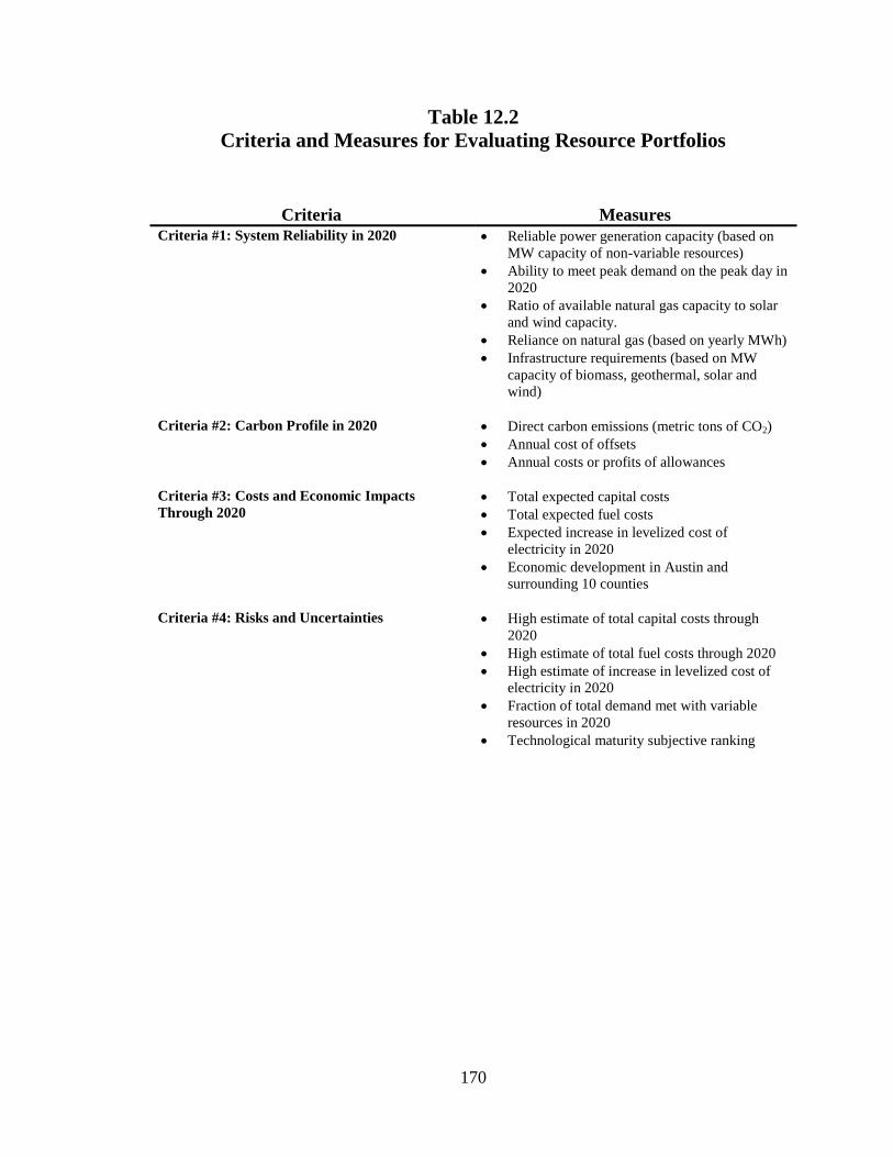
170

Table 12.2

Criteria and Measures for Evaluating Resource Portfolios

Criteria Measures

Criteria #1: System Reliability in 2020 Reliable power generation capacity (based on

MW capacity of non-variable resources)

Ability to meet peak demand on the peak day in

2020

Ratio of available natural gas capacity to solar

and wind capacity.

Reliance on natural gas (based on yearly MWh)

Infrastructure requirements (based on MW

capacity of biomass, geothermal, solar and

wind)

Criteria #2: Carbon Profile in 2020 Direct carbon emissions (metric tons of CO2)

Annual cost of offsets

Annual costs or profits of allowances

Criteria #3: Costs and Economic Impacts

Through 2020 Total expected capital costs

Total expected fuel costs

Expected increase in levelized cost of

electricity in 2020

Economic development in Austin and

surrounding 10 counties

Criteria #4: Risks and Uncertainties High estimate of total capital costs through

2020

High estimate of total fuel costs through 2020

High estimate of increase in levelized cost of

electricity in 2020

Fraction of total demand met with variable

resources in 2020

Technological maturity subjective ranking

171

Table 12.3

Measures of System Reliability (in 2020, rankings in parentheses)

Total Power

Generation

Capacity of

Non-Variable

Resources

(MW)

Fraction of

Peak Hourly

Demand Met

(%)

Ratio of

Unused

Natural Gas

Capacity to

Wind and

Solar

Capacity

Fraction of

Total Demand

Met with

Natural Gas

(%)

Total Power

Generation

Capacity of

Biomass,

Geothermal,

Solar and

Wind (MW)

Portfolio 1-AE

Resource Plan

2,976 (1)

100% (1) 1.58 (2) 14.6% (2) 1147 (1)

Portfolio 2-

Nuclear

Expansion

2,791 (4) 98.8% (6) 1.41 (4) 24.6% (4) 1147 (1)

Portfolio 3-

High

Renewables

2,374 (7) 100% (1) 0.50 (7) 4.6% (1) 3293 (7)

Portfolio 4-

Expected

Renewables

2,471 (6) 93.5% (8) 0.95 (5) 25.7% (5) 1388 (5)

Portfolio 5-

Renewables

with Storage

2,719 (5) 100% (1) 0.92 (6) 41.5% (7) 1388 (5)

Portfolio 6-

Natural Gas

Expansion

2,976 (1) 100% (1) 1.65 (1) 48.4% (8) 1147 (1)

Portfolio 7-

Cleaner Coal

2,976 (1) 100% (1) 1.57 (3) 15.6% (3) 1147 (1)

Portfolio 8-

High

Renewables

Without

Nuclear

1,952 (8) 97.3% (7) 0.38 (8) 26.7% (6) 3293 (7)

172

Table 12.4

Measures of Carbon Profile (in 2020, rankings in parentheses)

Direct Carbon

Emissions (metric tons

of CO2)

Annual Costs of

Offsetting Emissions to

Zero ($ million)

Annual Costs or

Profits of Allowances

($ million)

Portfolio 1-AE

Resource Plan

5,761,000 (8) 144 (8) -96 (8)

Portfolio 2-Nuclear

Expansion

1,646,000 (2) 41 (2) 55 (2)

Portfolio 3-High

Renewables

566,000 (1) 14 (1) 94 (1)

Portfolio 4-Expected

Renewables

3,993,000 (7) 100 (7) -31 (7)

Portfolio 5-Renewables

with Storage

2,984,000 (5) 75 (5) 6 (5)

Portfolio 6-Natural

Gas Expansion

3,021,000 (6) 76 (6) 4 (6)

Portfolio 7-Cleaner

Coal

1,791,000 (3) 45 (3) 49 (3)

Portfolio 8-High

Renewables Without

Nuclear

2,031,000 (4) 51 (4) 41 (4)

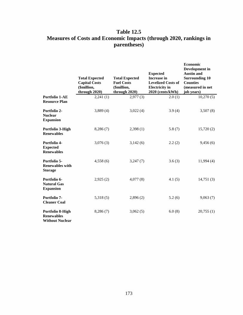
173

Table 12.5

Measures of Costs and Economic Impacts (through 2020, rankings in

parentheses)

Total Expected

Capital Costs

($million,

through 2020)

Total Expected

Fuel Costs

($million,

through 2020)

Expected

Increase in

Levelized Costs of

Electricity in

2020 (cents/kWh)

Economic

Development in

Austin and

Surrounding 10

Counties

(measured in net

job years)

Portfolio 1-AE

Resource Plan

2,241 (1) 2,977 (3) 2.0 (1) 10,270 (5)

Portfolio 2-

Nuclear

Expansion

3,889 (4) 3,022 (4) 3.9 (4) 3,507 (8)

Portfolio 3-High

Renewables

8,286 (7) 2,398 (1) 5.8 (7) 15,720 (2)

Portfolio 4-

Expected

Renewables

3,076 (3) 3,142 (6) 2.2 (2) 9,456 (6)

Portfolio 5-

Renewables with

Storage

4,558 (6) 3,247 (7) 3.6 (3) 11,994 (4)

Portfolio 6-

Natural Gas

Expansion

2,925 (2) 4,077 (8) 4.1 (5) 14,751 (3)

Portfolio 7-

Cleaner Coal

5,318 (5) 2,896 (2) 5.2 (6) 9,063 (7)

Portfolio 8-High

Renewables

Without Nuclear

8,286 (7) 3,062 (5) 6.0 (8) 20,755 (1)

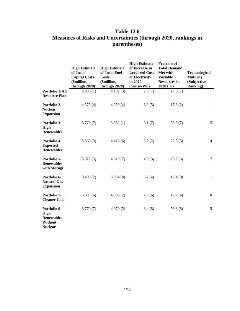
174

Table 12.6

Measures of Risks and Uncertainties (through 2020, rankings in

parentheses)

High Estimate

of Total

Capital Costs

($million,

through 2020)

High Estimate

of Total Fuel

Costs

($million,

through 2020)

High Estimate

of Increase in

Levelized Cost

of Electricity

in 2020

(cents/kWh)

Fraction of

Total Demand

Met with

Variable

Resources in

2020 (%)

Technological

Maturity

(Subjective

Ranking)

Portfolio 1-AE

Resource Plan

2,905 (1) 4,102 (3) 2.8 (1) 17.0 (1) 1

Portfolio 2-

Nuclear

Expansion

4,373 (4) 4,259 (4) 6.2 (5) 17.3 (2) 1

Portfolio 3-

High

Renewables

8,770 (7) 3,382 (1) 8.1 (7) 58.5 (7) 5

Portfolio 4-

Expected

Renewables

3,560 (3) 4,416 (6) 3.2 (2) 22.8 (5) 4

Portfolio 5-

Renewables

with Storage

5,072 (5) 4,619 (7) 4.9 (3) 23.2 (6) 7

Portfolio 6-

Natural Gas

Expansion

3,409 (2) 5,954 (8) 5.7 (4) 17.4 (3) 1

Portfolio 7-

Cleaner Coal

5,803 (6) 4,005 (2) 7.3 (6) 17.7 (4) 8

Portfolio 8-

High

Renewables

Without

Nuclear

8,770 (7) 4,370 (5) 8.4 (8) 59.3 (8) 5

175

Table 12.7

Comparative Ranking of Resource Portfolio Options

Portfolio

Rankings

System

Reliability

Score

Carbon

Emissions

and

Associated

Carbon

Costs Score

Costs and

Economic

Impacts

Score

Risks and

Uncertainties

Score

Total Score

(Average

Ranking)

Portfolio 1-

AE Resource

Plan

7 (1) 24 (8) 10 (1) 7 (1) 48 (2.75)

Portfolio 2-

Nuclear

Expansion

19 (4) 6 (2) 20 (5) 16 (2) 61 (3.25)

Portfolio 3-

High

Renewables

23 (5) 3 (1) 17 (2) 27 (6) 70 (3.50)

Portfolio 7-

Cleaner Coal

9 (2) 9 (3) 20 (5) 26 (5) 64 (3.75)

Portfolio 6-

Natural Gas

Expansion

12 (3) 18 (6) 18 (4) 18 (3) 66 (4.00)

Portfolio 4-

Expected

Renewables

29 (7) 21 (7) 17 (2) 20 (4) 87 (5.00)

Portfolio 5-

Renewables

with Storage

24 (6) 15 (5) 20 (5) 28 (7) 87 (5.75)

Portfolio 8-

High

Renewables

Without

Nuclear

36 (8) 12 (4) 21 (8) 33 (8) 102 (7.00)

176

Table 12.8

Costs of Reaching Carbon Neutrality

Direct

Carbon

Emissions

(metric tons

of CO2)

Total

Expected

Capital

Costs

($million,

through

2020)

Expected

Increase in

Levelized

Costs of

Electricity in

2020

(cents/kWh)

Metric

Tons of

CO2

Reduced

From 2007

Levels by

Million

Dollar

Invested in

Capital

Metric

Tons of

CO2

Reduced

From 2007

Levels by

Cent per

kWh of

Expected

Rise in Cost

of

Electricity

Expected

Total

Costs of

Offsetting

Carbon to

Zero ($

million,

through

2020)

Expected

Total Costs

or Profits of

Allowances

($million,

through

2020)

Annual

Costs or

Profits of

Allowances

($million)

Annual

Costs of

Offsets

($million)

Cumulative

Score and

Ranking

Portfolio 2-

Nuclear

Expansion

1,646,000 (2) 3,889 (4) 3.9 (4) 1140.94 (1) 1.137,720

(1)

1,424 (3) -31 (3) 55 (2) 41 (2) 22 (1)

Portfolio 3-High

Renewables

566,000 (1) 8,286 (7) 5.8 (7) 665.77 (6) 951,129 (2) 1,215 (1) 216 (1) 94 (1) 14 (1) 27 (2)

Portfolio 6-

Natural Gas

Expansion

3,021,000 (6) 2,925 (2) 4.1 (5) 1046.83 (2) 746,825 (6) 1,339 (2) 58 (2) 4 (6) 76 (6) 37 (3)

Portfolio 5-

Renewables with

Storage

2,984,000 (5) 4,558 (6) 3.6 (3) 679.85 (4) 860,764 (4) 1,516 (4) -163 (4) 6 (5) 75 (5) 40 (4)

Portfolio 7-

Cleaner Coal

1,791,000 (3) 5,318 (5) 5.2 (6) 807.07 (3) 825,382 (5) 1,621 (7) -297 (7) 49 (3) 45 (3) 42 (5)

Portfolio 4-

Expected

Renewables

3,993,000 (7) 3,076 (3) 2.2 (2) 679.36 (5) 949,865 (3) 1,611 (6) -282 (6) -31 (7) 100 (7) 46 (6)

Portfolio 8-High

Renewables

Without Nuclear

2,031,000 (4) 8,286 (7) 6.0 (8) 489.02 (7) 675,331 (7) 1,522 (5) -168 (5) 41 (4) 51 (4) 51 (7)

Portfolio 1-AE

Resource Plan

5,761,000 (8) 2,241 (1) 2.0 (1) 143.71 (8) 161,029 (8) 1,786 (8) -488 (8) -96 (8) 144 (8) 58 (8)

177

Figure 12.1

Metric Tons of CO2 Reduced From 2007 Levels by Cent per kWh of

Expected Rise in Cost of Electricity

AE Resource Plan

AE Resource Plan +

Nuclear

High Renewable Mix

Expected Renewables Mix

Expected Renewables +

CAES

AE Resource Plan + NG

AE Resource Plan + IGCC

w/ CCS

Replace both FPP and STP

with Heavy Renewables

0

1,000,000

2,000,000

3,000,000

4,000,000

5,000,000

6,000,000

0.0 1.0 2.0 3.0 4.0 5.0 6.0 7.0 8.0 9.0 10.0

Expected Increase in LCOE (cents/kWh)

Car

bo

n E

mis

sio

ns

in 2

02

0 (

met

ric

ton

s)

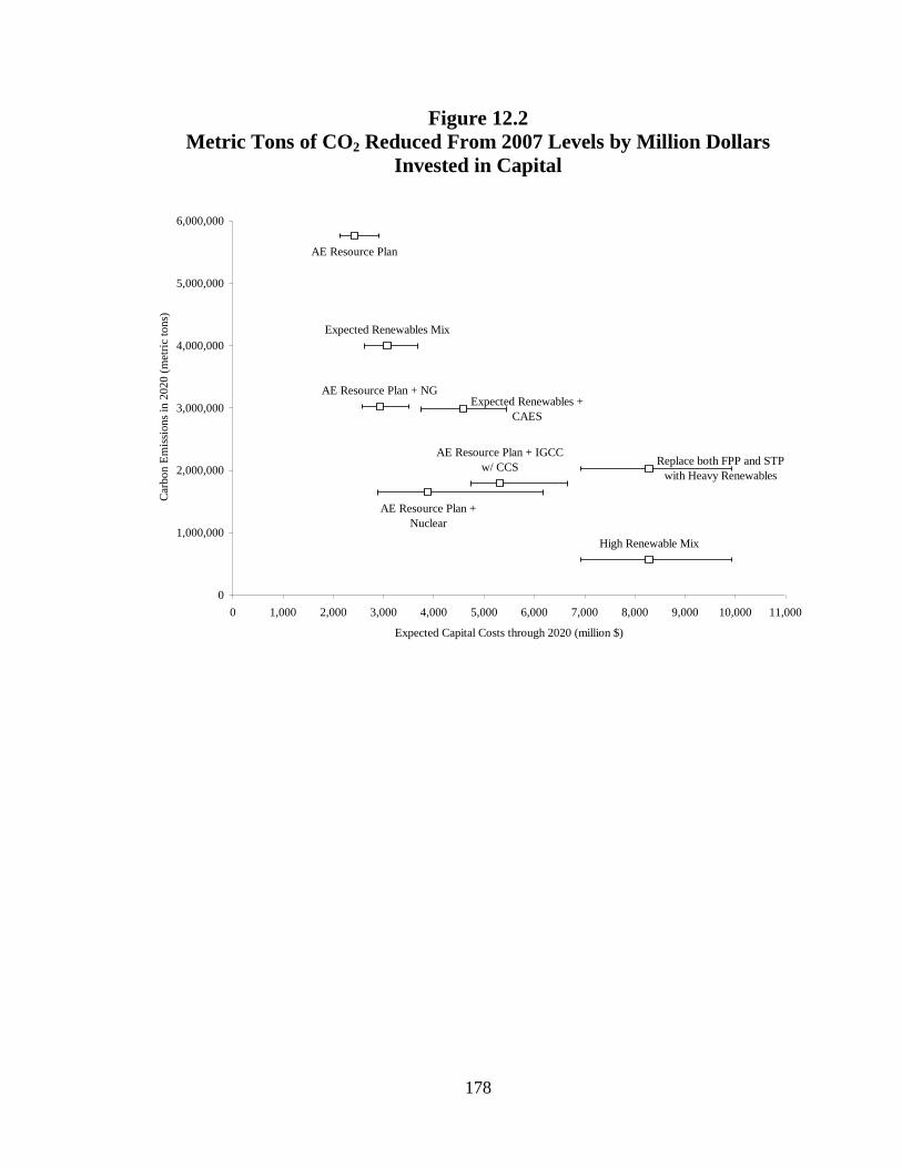
178

Figure 12.2

Metric Tons of CO2 Reduced From 2007 Levels by Million Dollars

Invested in Capital

AE Resource Plan

AE Resource Plan +

Nuclear

High Renewable Mix



CAES



w/ CCSReplace both FPP and STP

with Heavy Renewables

0

1,000,000

2,000,000

3,000,000

4,000,000

5,000,000

6,000,000

0 1,000 2,000 3,000 4,000 5,000 6,000 7,000 8,000 9,000 10,000 11,000

Expected Capital Costs through 2020 (million $)

Car

bon E

mis

sions

in 2

020 (

met

ric

tons)

179

Figure 12.3

Metric Tons of CO2 Reduced From 2007 Levels by Increase in Fuel

Costs

AE Resource Plan

AE Resource Plan +

Nuclear

High Renewable Mix



CAES



w/ CCS

0

1,000,000

2,000,000

3,000,000

4,000,000

5,000,000

6,000,000

0 100 200 300 400 500 600 700

Expected Fuel Costs in 2020 (million $)

Car

bon E

mis

sions

in 2

020 (

met

ric

tons)