Sustainable Private Native ForestryA review of timber production, biodiversity and soil and water indicators,

and their applicability to northeast New South Wales

RIRDC Publication No. 09/022

Sustainable Private Native Forestry

A review of timber production, biodiversity and soil and water indicators, and their applicability to northeast NSW

Alex Jay, David Sharpe, Doland Nichols and Jerry Vanclay

Southern Cross University Lismore NSW

March 2009

RIRDC Publication No 09/022

RIRDC Project No USC-8A

ii

© 2009 Rural Industries Research and Development Corporation. All rights reserved. ISBN 1 74151 827 X ISSN 1440-6845 Sustainable Private Native Forestry: A review of timber production, biodiversity and soil and water indicators, and their applicability to northeast NSW Publication No. 09/022 Project No. USC-8A The information contained in this publication is intended for general use to assist public knowledge and discussion and to help improve the development of sustainable regions. You must not rely on any information contained in this publication without taking specialist advice relevant to your particular circumstances.

While reasonable care has been taken in preparing this publication to ensure that information is true and correct, the Commonwealth of Australia gives no assurance as to the accuracy of any information in this publication.

The Commonwealth of Australia, the Rural Industries Research and Development Corporation (RIRDC), the authors or contributors expressly disclaim, to the maximum extent permitted by law, all responsibility and liability to any person, arising directly or indirectly from any act or omission, or for any consequences of any such act or omission, made in reliance on the contents of this publication, whether or not caused by any negligence on the part of the Commonwealth of Australia, RIRDC, the authors or contributors..

The Commonwealth of Australia does not necessarily endorse the views in this publication.

This publication is copyright. Apart from any use as permitted under the Copyright Act 1968, all other rights are reserved. However, wide dissemination is encouraged. Requests and inquiries concerning reproduction and rights should be addressed to the RIRDC Publications Manager on phone 02 6271 4165.

Researcher Contact Details Alex Jay Southern Cross University School of Environmental Science and Management Box 157 Lismore NSW Phone: 02 6620 3650 Fax: 02 6620 3492 Email: kiri@nor.com.au

Dr. Doland Nichols Southern Cross University School of Environmental Science and Management Box 157 Lismore NSW Phone 02 6620 3492 Fax 02 6620 3492 dnichols@scu.edu.au

In submitting this report, the researcher has agreed to RIRDC publishing this material in its edited form. RIRDC Contact Details Rural Industries Research and Development Corporation Level 2, 15 National Circuit BARTON ACT 2600 PO Box 4776 KINGSTON ACT 2604 Phone: 02 6271 4100 Fax: 02 6271 4199 Email: rirdc@rirdc.gov.au. Web: http://www.rirdc.gov.au Printing by Union Offset Printing, Canberra Electronically published by RIRDC in March2009

iii

Foreword The commercial and environmental values of private native forests have become increasingly important following reductions in log supply available from public forests, and with the realisation that achieving biodiversity conservation goals will require sympathetic management of the landscape matrix outside of the formal reserve system. This study reviews the forms of sustainability indicators such as standards and scoring systems that are relevant to private forests of the northeast NSW region. The research is a precursor to developing practical indicators which will help landholders and policy makers determine whether forestry management is likely to maintain or improve environmental outcomes, this being a key criterion in pending State legislation. However this research is independent of State government processes. This project was funded by the Natural Heritage Trust through the Joint Venture Agroforestry Program (JVAP), which is supported by three R&D Corporations — Rural Industries Research and Development Corporation (RIRDC), Land & Water Australia, and Forest and Wood Products Research and Development Corporation1 (FWPRDC), together with the Murray-Darling Basin Commission (MDBC). The R&D Corporations are funded principally by the Australian Government. State and Australian Governments contribute funds to the MDBC. This report is an addition to RIRDC’s diverse range of over 1800 research publications. It forms part of our Agroforestry and Farm Forestry R&D program, which aims to integrate sustainable and productive agroforestry within Australian farming systems. The JVAP, under this program, is managed by RIRDC. Most of our publications are available for viewing, downloading or purchasing online through our website: www.rirdc.gov.au. Peter O’Brien Managing Director Rural Industries Research and Development Corporation

1 Now Forest & Wood Products Australia (FWPA)

iv

Abbreviations ABARE Australian Bureau of Agriculture and Resource Economics AFS Australian Forestry Standard CMA Catchment Management Authority (NSW) CRA Comprehensive Regional Assessment (a joint assessment of forest values –

environmental, heritage, economic and social – undertaken by the Commonwealth and a State or Territory)

CSIRO Commonwealth Scientific and Industrial Research Organisation dEOAM draft Environmental Outcomes Assessment Methodology, a regulation

under NVA ES(F)M Ecologically Sustainable (Forest) Management FSC Forest Stewardship Council FWPRDC Forest and Wood Products Research and Development Corporation GIS Geographic Information System LGA Local Government Area LNE lower northeast region of NSW MPIG Montreal Process Implementation Group MC& I Montreal Criteria & Indicators NSW New South Wales NVA the NSW Native Vegetation Act 2003 PNF private native forests or forestry as the context suggests s.d. standard deviation of a sample SE standard error of a sample mean SEQ southeast Queenland Qld Queensland R&D Research and Development RFA Regional Forest Agreement RIS Regulatory Impact Statement SFM Sustainable Forest Management (S) FNSW Forests New South Wales UNE upper northeast region of NSW

v

Contents

Foreword ...................................................................................................................................iii

Abbreviations ............................................................................................................................ iv

Contents...................................................................................................................................... v

Executive Summary .................................................................................................................vii

Introduction ................................................................................................................................ 1

1. Sustainability definitions........................................................................................................ 1

2. PNF in northeast NSW........................................................................................................... 5

3. The legal and policy context .................................................................................................. 8

4. Certification and standards................................................................................................... 13

5. Biodiversity indicators ......................................................................................................... 16 5.1 What is Biodiversity? ..................................................................................................... 17 5.2 What is Habitat ? ............................................................................................................ 18 5.3 Population Size and Conservation.................................................................................. 19 5.4 Surrogate Species ........................................................................................................... 20

6. Habitat value, site attributes, and spatial and environmental effects ................................... 23

7. Resolving the use of fauna indicators .................................................................................. 27

8. Effects of timber harvesting ................................................................................................. 29

9. Timber production indicators ............................................................................................... 30 9.1 Sustainable silviculture: maintaining an even flow of timber........................................ 30 9.2 Forest condition and removals; regeneration and gap size ............................................ 31 9.3 Economics of stand rehabilitation .................................................................................. 33

10. Soil and hydrological processes ......................................................................................... 38 10.1 The role and function of stream buffers ....................................................................... 38 10.2 Area of stream buffers in UNE NSW PNF .................................................................. 41 10.3 Soil management .......................................................................................................... 42

11. Uncertainty and risk management...................................................................................... 43

12. A comparison of three structural and landscape indices for biodiversity value and sustainability............................................................................................................................. 46

12.1. The Habitat Hectares (HHa) approach ........................................................................ 48 12.2 Biodiversity Benefits Index BBI .................................................................................. 49 12.3 PVP developer and the BioMetric score ...................................................................... 53

13. Adaptive management........................................................................................................ 57

14. Towards an improved index of sustainability .................................................................... 58 14.1 Rationale for, and form of a sustainability index ......................................................... 58 14.2 Integrating time effects in the sustainability index ...................................................... 62 14.3 Conclusion.................................................................................................................... 65

15. References .......................................................................................................................... 66

vi

List of Figures (note Figures and Tables are numbered according to the sections they appear in the document) Figure 1 Components and Process of Sustainable Forest Management. ..................................... 2 Figure 2 Northern Rivers Catchment Management Authority area............................................. 5 Figure 3 Native forest wood supply in NE NSW ........................................................................ 6 Figure 6.1 Maximum combined spatial and structural heterogeneity in a logged landscape ...... 24 Figure 6.2 Fauna & Habitat correlation ....................................................................................... 25 Figure 9.1 A representative stand structure for mixed-age Spotted Gum forest. ......................... 33 Figure 9.2 Annual growth in value in a simulated stochastic mixed-age

Spotted Gum forest stand ............................................................................................ 34 Figure 9.3 Outcome from EUCAMIX model indicating stand development under three

silvicultural regimes. ................................................................................................... 34 Figure 14.2.1 Site scoring for BBi over time: ................................................................................... 62 Figure 14.2.2 Site scoring for two sites ............................................................................................. 63 Figure 14.2.3 Site scoring showing biodiversity credit and debit ..................................................... 64 List of Tables Table 4: excerpts from AFG checklist for compliance with AFS ............................................. 14 Table 9 Mean NPV outcomes ($/ha) for three silvicultural treatments.................................... 35 Table 12.2.1 Weightings used in BBI vegetation condition score V. .............................................. 51 Table 12.3.1 Vegetation associations. .............................................................................................. 54 Table 12.3.2 The “PVP developer” BioMetric scoring system........................................................ 56 Table 14.1 Passport scoring approach for wildlife-BBi ................................................................ 61

vii

Executive Summary

What the report is about Private Native Forests are a dominant part of the landscape in northeast NSW and their future is a matter of great debate. Private Native Forests are an essential component in the supply of building materials to the public, and have historically contributed significantly to regional economic activity. These contributions have been made from the matrix of managed and reserved lands that also provide a complex array of environmental benefits. Sustaining the flow of these benefits is important for landowners, timber and tourism industries, and regional communities in northeast NSW. In recent decades society has expressed concerns about how to integrate forest management techniques for timber production with those that improve the condition of the physical and biological environment. This report reviews our knowledge base of native forest silviculture in this region, including what is known about the current condition of private native forests. Secondly, the report reviews the use of indicators of sustainable maintenance of habitat and discusses their major strengths and weaknesses. Who is the report targeted at? The report should be read by those interested in understanding the general nature of private native forests in northeast NSW and in the management regimes that have led to their current state. The report also should be read by those with an interest in developing habitat and landscape indices for planning and valuation purposes, including wildlife researchers, forest managers, and policy makers. Aims/Objectives The aim of the research is to provide background information that will inform the development of a sustainability index for private native forestry to be used by landowners, stewardship incentive program managers, and standards compliance assessors. We aim to develop a standard of care for native forests that incorporates the knowledge base that has been accumulated in the forest and biological sciences. Methods used The report describes private native forests in northeast NSW and their legislative context, and reviews the use of standards and scoring methods as sustainability indicators, with a particular focus on the differences among the various indices. The effects of timber harvesting practices on fauna, timber production and soil and water processes are discussed, and an efficiency-based approach for dealing with the uncertainties prevalent in long-term resource management is described. Results/Key findings Sustainability is a dynamic process and cannot be measured by a snapshot view. Within-forest variation across time and spatial scales is desirable to maintain a diversity of habitats, but this leads to problems in reliably detecting long-term trends. Ongoing monitoring is expensive and should be targeted to areas of key concern. Standards are most useful as strategic planning and basic operational “harm-prevention” tools, but do not encourage outcomes above a lowest common denominator. Scoring methods are more relevant for operational-level assessments and to measure trends over time and if appropriately linked to stewardship rewards, can encourage general improvement and promote the most efficient outcomes. Although correlation between habitat attributes and fauna presence is of

viii

low precision (the presence of suitable habitat does not guarantee presence of targeted fauna), an objectively-scored coarse filter approach fits well with precautionary principles and can be used to prioritise action among sites. Current scoring methods are based on before-and-after site conditions, and are not well suited for forestry operations which involve dynamic forest structures and conditions. Implications for relevant stakeholders Landowners have to make management decisions about a dynamic system (i.e. the forest) in a complex environment of personal, financial, and legal conditions. By adopting the use of sustainability indicators which account for dynamic forest development and point towards broadly desirable outcomes, landowners can reduce some of this complexity and will be better equipped to adopt a planning and adaptive management framework focussed on their objectives, that will also include environmentally sustainable outcomes. The community – through work on specific pieces of forest - will have more visible indications that private native forests are being responsibly and sustainably managed. Policy makers and strategic planners will have a greater resource of information to use, and will be better able to choose and prioritise between alternative actions. Recommendations The second phase of this research aims field test some different forms of indicators in the widespread, commercially important dry Spotted Gum forest type, and develop a “toolkit” to simplify the measurement and interpretation of the indicators. The outcomes of this exercise will be relevant to landowners and policy makers, who need specific measures they can use to distinguish well-managed from poorly-managed or abandoned forests.

1

Introduction The direction of management of the vast private native forestry estate in NSW is an important and contentious issue. The purpose of this review is provide theoretical and practical guidance for assessing the maintenance of biodiversity, timber production and soil and water values in private forests in the northeast region of NSW. The SCU research team has proposed developing and field testing an index of sustainability, based on the information in this review.

1. Sustainability definitions There is currently great discussion of “sustainability” across all realms of society. Concerns fall into the environmental, social and economic spheres and the goal in most consideration of sustainability is to define how to balance these three elements in a given system. Sustainable forestry is presently defined by use of criteria and indicators. “The criteria are general principles that express commonly agreed upon objectives…., while the indicators are designed to assess whether these objectives are being met” (Brand 1997, cited by Di Stefano 2001). A well-known and widely-adopted example is the Montreal Criteria and Indicators (MC&I). MC&I in turn provide the basis for the Australian Forestry Standard (AFS) which is a quality assurance scheme to certify that participants are following particular processes in forest management. Under the Montreal Process sustainable forestry is achieved when these goals are met:

• Maintenance of productive capacity of forest ecosystems. • Maintenance of forest ecosystem health and vitality. • Conservation and maintenance of soil and water resources. • Maintenance of forest contribution to global carbon cycles. • Maintenance and enhancement of long-term multiple socio-economic benefits to meet the

needs of societies. • There is a legal, institutional and economic framework for forest conservation and sustainable

management. One of the most common concepts of sustainability is that of a steady “flow” of services or materials derived from “stocks” of natural resources. The idea of outputs in perpetuity is intuitively reasonable, but needs to be qualified with the condition that such outputs do not arise from running down the capital stock, eg harvesting faster than growth rate. Sustainability is therefore by definition dynamic, and cannot be measured by snapshot views of the resource or system being considered.

2

The process of assessing sustainability is a cycle and suitable indicators are context-dependent (Vanclay 1995), as illustrated in Figure 1 based on Di Stefano (2001) and Chesson (2002)

Change Don’t change

Figure 1 Components and Process of Sustainable Forest Management. Identifying the core objectives is important at the outset so that the indicators don’t become a defacto goal in themselves. Furthermore, indicator measures must be practical to collect and monitor and have meaning and benefit for the land managers who will ultimately be using them. Achieving a balance between simplicity and accuracy is an ongoing challenge. The critical level of change that triggers management changes, and the probability and cost of correctly detecting it, are issues that need wider recognition (Di Stefano, 2001). Long a focus of forest management, as opposed to forest exploitation, has been the concept of “sustained yield”, meaning that the forests of a region or country should not be harvested at a rate greater than their growth. The idea of outputs in perpetuity is embedded in the phrases “sustainable development” and “ecologically sustainable forest management” (ESFM) and while various definitions of these focus on either end-points or on processes, most incorporate the “triple bottom line” of environment, economy and social conditions. “Sustainable development” embodies the broader idea of tradeable (fungible) natural, social and economic capital (Pearce & Turner 1990) whereas ESFM would initially seem to be more focussed on flows and stocks within the boundaries of a geographically defined biological system. However this seeming distinction between ESFM and SD may be misleading. In Australia, ESFM definitions start from the 1995 National Forest Policy Statement (Anon 1995) where the broad principles of ESFM have been summarised as [ RFA (2000 ) ; Attachment 14 ]:

• Maintain or increase the full suite of forest values for present and future generations across the NSW native forest estate. Aims for values include biodiversity; the productive capacity and sustainability of forest ecosystems; forest ecosystem health and vitality; soil and water; positive contribution of forests to global geochemical cycles; long term social and economic benefits; natural and cultural heritage values.

Define sustainable forestry objectives

and goals

Social values Ecological values Economic values

Select indicators that measure status of

criteria & goals

Implement monitoring program

Test for change in indicators

Subdivide the goals until measurable operational

criteria are possible

Aggregate lower level indicators to form a core set for assessment and reporting

without destroying information

content

Establish baseline levels and critical change levels to trigger action

Forest management

practices

Management Decision

3

• Ensure public participation, access to information, accountability and transparency in the delivery of ESFM.

• Ensure that legislation, policies, institutional framework, codes, standards and practices related to forest management require and provide incentives for ecologically sustainable management of the native forest estate.

• Apply precautionary principles for prevention of environmental degradation. • Apply best available knowledge and adaptive management processes.

Indicators are indirect or proxy measures for assessing whether goals are being attained. Indicators of sustainability have been used at a range of scales from the broad national level (Yale Univ CELP, 2005) to specific resource elements in a particular context, for example plantation soil management (Carlyle et al 2003). Since it is not possible to monitor or measure everything, or even measure some items directly (e.g. “conservation of biodiversity”), ESFM can only be implemented by having measurable, scientifically valid indicators of progress or outcomes. However given the broad objectives, such indicators are, not surprisingly, difficult to formulate. In this review we have adopted the position that assessing sustainability is best done as a scientific, positive, objective process, while moral philosophy or normative value judgements create the social context from which management goals are derived. The Australian State and Federal parliament’s views of the essential aspects of ecologically sustainable development might perhaps best be gauged from statutory definitions of this term. These are to be found in (i) Sect 6(2) of NSW Protection Of The Environment Administration Act 1991 (POEAA) from whence the definition is carried across into other Acts including the Native Vegetation Act (NVA) 2003, and (ii) Sec 3A of the Commonwealth Environmental Protection and Biodiversity Conservation Act 1999 (EPBCA). In summary the definitions encompass

(a) the precautionary principle - notwithstanding scientific uncertainty, avoid irreversible damage by considering risk-weighted consequences

(b) inter-generational equity - ensure a full range of options is available to future generations (c) conservation of biological diversity and ecological integrity- a fundamental consideration (d) improved valuation, pricing and incentive mechanisms- environmental factors should be

transparently valued in pricing of assets and services Thus both Commonwealth and State legislation indicate four primary principles of sustainability. The Commonwealth also says “decision-making processes should effectively integrate both long-term and short-term economic, environmental, social and equitable considerations” ( EPBCA 1999 sec 3A), and the clause in the NSW State Act (POEAA 1991) concludes … environmental goals, having been established, should be pursued in the most cost effective way, by establishing incentive structures, including market mechanisms, that enable those best placed to maximise benefits or minimise costs to develop their own solutions and responses to environmental problems. Clearly, parliament has perceived that equity and efficiency are important elements of ecologically sustainable development, and that regulatory mechanisms alone will be ineffective. ESFM is a primary driver of public forest management in the Upper North East (UNE) region of NSW (SF NSW 2004, 2005). The NSW government has also confirmed its commitment to “the achievement of [ESFM]… on Private Land …” (clause 46, RFA 2000). The signed RFA document further noted that arrangements for attaining ESFM on private lands would comprise

• a process of encouragement of private landowners (cl. 55), • a Code of Practice for PNF (cl. 57), • voluntary participation by landholders in schemes to achieve conservation objectives (cl. 56),

4

and that conservation levels achieved in the Comprehensive, Adequate and Representative (CAR) reserve system on public lands would not be used as a basis for preventing timber harvesting on private lands (cl. 59). Broadly, the assessment of socio-economic sustainability of forest land use decisions include various permutations of Benefit-Cost Analysis taking into account market and non-market values (e.g. Sinden & Worrell 1979). It is not proposed to go into detail on those aspects in this review; Jay (2005a) provides an overview. Some further comment on economic aspects of sustainability is in section 10. (‘Uncertainty and risk management’).

5

2. PNF in northeast NSW The discussions in this report are relevant to the area of NSW from about Port Macquarie to the Queensland border, and inland to the New England Highway. This includes the Northern Rivers Catchment Management Authority (CMA) Area (Figure 1), which in turn encompasses the northern third of the Lower North East (LNE) Regional Forest Agreements (RFA) area and all except some western parts of the Upper North East (UNE) NSW. Figure 2 Northern Rivers Catchment Management Authority area (source http://www.cma.nsw.gov.au/)

Approximate division between upper

northeast and lower northeast RFA regions

6

Projected Wood Supply from northeast NSW (UNE + LNE) public forests (SFNSW 2005)

0

200,000

400,000

600,000

800,000

2005

2015

2025

2035

2045

2055

2065

2075

2085

2095

An

nu

al V

olu

me

(m3

) f

or

5 y

ear

per

iods

plantation

native

-

100,000

200,000

300,000

400,000

500,000

1975 1980 1985 1990 1995year

m3/yr

Private UNEState ForestsHQLHQS

LQPNF une+lne

Native ForestHardwoodsupply ;

UNE+LNE(DAFF,

Private Native Forestry (PNF) is a significant economic and land use activity in the region. In 1999 some 40% of the 450,000m3/ annual hardwood log intake of the UNE region’s mills was being sourced from private land. Public forest supply has declined substantially since the early 1990’s and is projected to decline sharply again in about 20 years or less as shown below. High Quality Large (HQL) logs are likely to constitute progressively less of the total volume over time. Figure 3 Native forest wood supply in NE NSW (a) actual (b) projected from public forests Total employment in the hardwood timber industry sector in NE NSW was around 1200 persons excluding private native forest landowners, and the industry contributed some $220M annually to the regional economy in the form of timber, wages, value-adding and other payments (CARE et al 1999). However the private log supply is on a steep downward trend in both UNE and LNE, having halved between 1975 and 2000. Countering this trend are short term spikes in private log supply which have occurred as a response to withdrawals of public forest from the production estate. (DAFF 1999a). The private native forests of the region are comparable in extent to the public forests (State Forest, National Park, Nature Reserves and Crown Land combined); PNF is in fact slightly larger than the public forest area in UNE. About 60% of the combined UNE and LNE land area (9.7M ha) has forest cover (5.6M ha), and about two-thirds of the forest cover on all tenures is potentially productive native eucalypt forest types (3.8M ha). Nearly half of this (1.7M ha) is privately owned, being divided about 0.8/0.9M ha between UNE/LNE respectively (Keenan and Ryan 2005). Dry Spotted Gum (Corymbia maculata, C. variegata and C. henryi) and Dry Blackbutt (Eucalyptus pilularis) broad forest types comprise about a third of the potentially productive private forest, and these two species provided about half of the total (public and private) log volume supplied to mills in the late 1990’s. (DAFF et al 1999). Spotted gum logs are more predominant in the north and blackbutt in the south. In 1998 there were around 145 licensed sawmills in the UNE area. Fifty-five of these receive Crown logs and of those, only 8 receive>10,000m3/yr, and 28 receive< 1000m3/yr (Fortech 1999). The intake of one large company (Boral Ltd) amounts to ~ 60% of the total Crown supply. Most larger sawmills supplement their State Forest allocations with private property resource, whilst a large number of small mills rely totally on private forestry harvests. Nearly three-quarters of the public forest

7

hardwood sawlog sales are for floorboards (42%) and house framing (22%) and other dry structural products (11%) (FNSW 2004). A number of studies have considered economic development opportunities, supply scenarios, and the role of PNF in the regional economy. These include CARE et al (1999), Fortech (1998), NNFS (1994, 1999, 2000, 2002), MGP, Powell and James (1995), DSD (NSW Dept State Development) (1989) CARE et al. (1999) has detailed socio-economic and statistical information including regional input/output matrix, employment and value multipliers. Compiling various figures from these reports suggests that around two-thirds of the total potential current private sawlog and roundwood supply is currently being made available to industry by landowners in the UNE region, which translates to an annual average (sawlogs & other roundwood only) yield of 0.8 to 1.0m3/ha/yr from a net production estate (after accounting for intent, accessibility and net harvestable area) of around 150,000 to 180,000 ha in UNE region (Jay 2005 in prep c). Jay (2005a) reports on landowner management intent for the UNE region, and estimates an upper limit of annual harvested area (selection harvest not clearfell) to be at most about 12,400 ha or 1.0% of the gross PNF estate. Data is no longer kept by State Forests of NSW on the annual volume of logs that mills source from private forests. Sustainable future supply is dependent not only on the net available area of the forest but also its silvicultural condition and non-declining biophysical conditions. The PNF estate is in generally poor productive condition, having had a long history of indifferent management and/or high-grading, meaning removal of commercial stock without due attention to silvicultural improvement treatment. Jay (2005c) found that the most common structure in inventoried PNF plots in Spotted Gum and Blackbutt types was one where the predominant biomass (basal area) class was trees 10-25cm diameter, with very few trees in the >70cm DBH classes. However Keenan and Ryan (2004) list 234,000 ha of UNE PNF or some 20% of the total private forest as old-growth (i.e. predominantly mature forest where effects of disturbance are now negligible and regrowth cover is less than 30% of total). They also note that 371,000 ha of old-growth or 57% of the total 655,000 ha area of old-growth on both public and private land, is in formal and informal reserves. Both of these contrasting structures are relevant to future supply, since the poor silvicultural condition of the regrowth dominated stands means they are unlikely to be a source of significant volumes of timber for some time (especially the high quality large logs which are in short supply), and regulatory constraints may prevent harvest in old-growth stands. Private forests in northeast NSW are also important for their conservation, biodiversity, water quantity and quality, landscape aesthetics and other environmental values. However as non-market, non-excludable products (i.e. goods or services), the continuing supply of these values (products) from private land is dependent on either (i) landowners managing their forests to supply their own demand for the products, (ii) the development of market systems to generate value from the products, or (iii) regulatory systems to coerce, control or command supply of the products. Young et al (1996) have comprehensively discussed voluntary market-based instruments to promote conservation of biodiversity. Markets for ecosystem services are the subject of a scoping study by Binning et al (2002), and are also discussed by ABARE (2001), van Bueren (2001) and The Productivity Commission (2004). Pannell (2004) provides perhaps the most accessible and comprehensive introduction. Figgis (2004) suggests that the role of market incentives is to reward provision of valuable services, not to provide compensation for a hands-off prescription. Gillespie (2000) cites some costs of native vegetation ownership on private land in NSW; direct costs of managing remnant vegetation in the Riverina averaged around $2400 per annum per property, and for 89% of landholders the sum of direct plus opportunity costs of native vegetation retention exceeded agricultural productivity or other directly marketable benefits obtained on site. Pilot incentive-based schemes have been trialled in NSW, but prescriptive regulation appears to be the most likely form of government interventions in PNF in NSW (DIPNR, 2004).

8

3. The legal and policy context Private native forest harvesting or other silvicultural action in NSW is regulated primarily under the Native Vegetation Conservation Act 1997 (NVCA). Harvesting on steep land (>180 slope) or other protected land is subject to approval and conditions set by the Department of Natural Resources (DNR, formerly DIPNR). Although the NVCA was repealed by Parliament in December 2003 and replaced by a new Native Vegetation Act (NVA 2003), this is yet to be gazetted so the provisions of the 1997 Act continue. Under the NVCA, where a Regional Vegetation Management Plan is not in force, as is the case for the northeast, some forms of “clearing” continue to be exempt from the NVCA 1997 under transitional provisions in that Act retained from State Environmental Planning Policy SEPP 46 Schedule 3. These exemptions include

(i) The clearing of native vegetation in a native forest in the course of its being selectively logged on a sustainable basis or managed for forestry purposes (timber production).

There are no statutory definitions of the meaning of “sustainable” in this context, and the interpretation of this provision is subject to guidelines issued by DIPNR. These state, inter alia,

Selectively logged on a sustainable basis is taken (as adapted from Smith and van der Lee 1992 [ref unknown]) to be felling and removal of part of a forest for the purpose of selective timber production which, at a minimum, maintains:

• habitat value; • an uneven age forest structure; • more than 50% retention of trees greater than 40 cm dbh (diameter at breast height)

on a broad area basis in each logging cycle; and • the forest in a state from which it can recover to a similar structure before next

logging cycle. ……To be eligible to claim this exemption, therefore, it would be reasonable to expect a private- native forest owner to be able to furnish evidence of the application and accomplishment of these sustainable land practices through some form of forest management plan…… ……This means that there should be clear evidence of the continuous passage or progress through time of a succession of stages of forest management practices……. (http://www.privateforestry.org.au/exempt4.htm )

“Sustainable” practices are thus prescribed by an administrative interpretation rather than by Parliament, with a strong if not mandatory need for documentary support and evidence of intent. As far as is known, has not been tested in the courts. Northern Rivers Private Forestry Development Committee cautiously considers that

…….By and large the current exemptions do not cover normal forestry operations such as selective logging… http://www.privateforestry.org.au/private_nat_for_res_ntnsw4.htm

This current status of exemption by administrative interpretation was clearly never intended to be a long-term provision. The NVCA intended that Regional Plans would eventually supercede the SEPP 46 provisions, however the draft Plans were highly controversial and the NVCA was repealed prior to their gazettal as a regulation. Only two, Riverina-Highlands and Mid-Lachlan, appear to have become statutory instruments (http://www.austlii.edu.au). Prior to the introduction of the new Act, a working group of appointed members of the public, NGOs and government agencies produced a report recommending the adoption of a Code of Practice for PNF and the form this might take

9

Currently forest landholders are encouraged to follow the “Interim Best Operating Standards for Private Forest Harvesting”,(http://www.dipnr.nsw.gov.au/nativeveg/plantations/pnf.shtml 42pp); however this document has no legal force except where it is attached as a condition for harvesting on Protected Land or on a “clearing approval” when landholders make an application under the NVCA 1997 if they are uncertain about or unable to exercise the “sustainable forestry” exemption. The more contentious conditions of the proposed Code include

• Requirement to prepare detailed forest management and harvest plans • Continued responsibility to survey/manage for Threatened Species • Riparian buffer zones from 10 to 40m • Retention of minimum basal areas 12-18m2/ha depending on site height • Retention of habitat trees and recruits additional to those in buffers or unlogged areas. • Associated additional costs of planning, operations, and loss of management control and

sovereignty The NVA 2003 was passed in the same parliamentary session as legislation which created Catchment Management Authorities. CMAs are appointed boards with statutory responsibilities for planning and implementing natural resource policies. A major role of the CMAs will be to approve or modify Property Vegetation Plan (PVP) applications. Submitting PVPs is voluntary, but once approved they become binding on the title for a term of 15 years and may only be varied with the Minister’s consent. PVPs determine vegetation management on the property in that period. It is still unclear whether the NSW government intends that the CMA be a determining authority for PNF proposals within a PVP, or whether this role will be retained by DNR. In the Minister’s second reading of the Act, he said…

The Hon. MICHAEL COSTA (Minister for Transport Services, Minister for the Hunter, and Minister Assisting the Minister for Natural Resources (Forests)) I will take this opportunity to explain how the Government intends to deal with the issue of private native forestry. It is intended that a regulation will be made to include a code of practice for private native forestry. If private native forestry operations conform with that regulation, a PVP will be approved. The code of practice will be developed in full consultation with PNF stakeholders including the growers. Conforming operations should be able to be processed quickly. If necessary, interim arrangements can be established through the regulations to continue the current exemption under the Native Vegetation Conservation Act 1997 until the new arrangements are in place. Using this approach, the Government aims to avoid disrupting current operations, particularly those on the North Coast. (NSW LEGISLATIVE COUNCIL Hansard, Page: 5947 Friday 5 December 2003 http://www.parliament.nsw.gov.au/prod/parlment/hansart.nsf/a60a6a8d2db7ace1ca256e6a0024cf47/de871b888ec6a4ffca256dfd002147a8!OpenDocument )

Following the passing of the NVA 2003, a new group was formed to revisit the formulation of a Code under this new Act,. This group met throughout 2004 without coming to agreement on basic matters, including acceptable numbers of hollow trees and minimum basal areas to be retained. The original group has not been reconvened since October 2004. However according to DNR a draft Code of Practice for PNF is continuing to be developed .(http://www.dipnr.nsw.gov.au/nativeveg/plantations/pnf.shtml – accessed November 3, 2005).

10

The overarching principle in NVA 2003 is that any clearing is only to be permitted if it “improves or maintains environmental outcomes” ..“in accordance with the principles of ecologically sustainable development” (NVA 2003 sec 3(b) ). The intention is that landholders who operate in accordance with a PNF Code under the Act will be deemed to be automatically complying with this principle. An assessment of whether other clearing (including forestry operations not in accordance with the PNF Code) meets the “maintain or improve” test is to be a carried out using a defined methodology (draft Environmental Outcomes Assesssment Methodology, henceforth dEOAM). dEOAM will be given statutory authority by reference from the Native Vegetation Regulations (NVR sec 18[2]) which have been made under part 32(b) of the Act (NVR Part 5 secs 18 & 20). The NVA 2003 distinguishes between “regrowth” and “remnant” vegetation, and generally only applies restrictions to clearing of remnant vegetation. In the northeast region, remnant vegetation is defined (sec 9 ) either as that which has regrown since 1990, or since another date specified in a PVP. This differs from the generally understood definition of “regrowth” forest as that which has grown since abandonment of human-cleared areas. However the NVR (sec 9) permits a PVP to vary this date only if there has been two occasions of clearing “pursuant to existing rotational farming practices” since 1950. Sec 9(3)(a) of the Act defines the latter as those “that are reasonable and in accordance with accepted farming practice”. It is unclear whether “rotational farming” includes intermittent sustainable forestry harvest, although clearly PNF has not been specifically or purposefully included. The dEOAM has an extensive list of forest types (“Keith Formations”, Appendix D in dEOAM) grouped by CMA region in which any “broadscale clearing” will be prohibited if less than 30% of the original extent remains. Of the potentially commercial forest types in this category in UNE NSW, most are tableland occurrences (Stringybark, Peppermint, Brown Barrel, Messmate and Manna Gum types); Swamp Mahogany is the only affected coastal type. If the Act and current general draft regulation are gazetted without a PNF Code, it thus appears that PNF will be immediately subject to the same general provisions as all other “broadscale clearing”. As will be noted later , the effect of this would be to make PNF immediately inoperable. The legislative power to make separate specific provision for a PNF Code appears to be possible either (i) under sec 32(b) of NVA whence the present NVR and dEOAM have been derived, but noting that these do not currently exclude PNF, or (ii) declaring PNF to be a conditional “routine agricultural management activity” under Sec 11(2) of the new Act. Various aspects of a prescriptive regulatory Code do not appear to conform with other policy directions taken earlier by the State government. The NSW Cabinet office (1995) states…..

The removal of overly prescriptive provisions...is consistent with the government policy for more efficient regulation established by the Regulatory Review Unit of the NSW Cabinet Office. The best practice approach requires that regulatory proposals:

• have clear objectives and focus on fixing identified problems • regulate ends not means • maximise benefits and minimise costs • are integrated with other regulatory systems so that the public is presented with

requirements that 'make sense' across government as a whole • minimise the number of government agencies involved • promote certainty (so that the assessment of applications for approvals, permits,

licences, etc is based on clearly stated criteria and the timeframe for the assessment process is indicated publicly)

• are simple for the users to understand • are simple to administer • are easy to enforce

11

• have a high voluntary compliance rate • are subject to regular review • do not restrict competition • use commercial incentives rather than command and control rules, for example by:

o information provision o encouraging voluntary compliance backed up by a statute only where

necessary o attaching monetary value to reduction in environmental harm o tying the long-term commercial interests of natural resource harvesters to

their current management of the stock o providing accessible legal remedies so that consumers, rather than

government, can act to enforce their rights without prohibitive costs The above is an edited extract from a 1995 NSW Cabinet Office publication: “From Red Tape to Results - Government Regulation: A Guide to Best Practice”, which was the subject of “Memorandum 95-11; Regulatory Reform- Memorandum to all Ministers”, an instruction from the Premier Mr Carr to adopt such criteria in the interests of best practice regulation.

These form a suitable set of criteria against which to evaluate a draft PNF Code. Other legislation which has direct impact on management of PNF include the NSW Environmental Planning and Assessment Act 1979 as amended (EPAA), and the NSW Threatened Species Conservation Act 1995 as amended (TSCA). The EPAA defines protocols for assessment of development applications which are referred to in NVA, but otherwise is relevant principally in that it allows continuance of existing lawful use (Sec 107[1]), notwithstanding a change in any environmental planning instrument which may affect the land. However a burden of proof may rest with the landowner who wishes to claim an existing use of intermittent forestry operations, since Sec 107 [3] states that “a use is to be presumed, unless the contrary is established, to be abandoned if it ceases to be actually so used for a continuous period of 12 months.” Whether a forest is “used” for production while growing between cutting cycles has not been tested in the courts. Changes of scale or intensity of use are specifically denied under the existing use provision. The TSCA aims to prevent development activities significantly damaging listed “threatened species [both animal and vegetable], populations and ecological communities” A significant impact triggers a Species Impact Statement (SIS) which will usually explain or propose some mitigating modifications to the proposal or compensatory offset actions. The burden of proof is on the proponent of the activity to demonstrate by means of an eight-part test (sec 94) that there will not be any significant impacts from the proposed activity. Specific activities may also be listed as “key threatening processes”. Forestry per se is not included in this list but certain listed threatening processes are relevant (e.g. clearing of native vegetation, removal of dead wood and dead trees, high fire frequency; Sched 3 TSCA) The Commonwealth Environment Protection and Biodiversity Conservation Act 1999 (EPBCA) relates to biodiversity issues on a national scale, irrespective of land tenure. Developments and/or activities that are likely to have a significant impact on listed species, communities and heritage areas must be referred to the Commonwealth Minister for the Environment for approval. However forestry operations conducted under a Regional Forest Agreement are exempt from EPBCA 1999 (sec 38, with some exceptions not relevant to PNF). Continuation of lawful pre-existing uses is also exempt (sec 43B). An RFA forestry operation is by definition one which occurs in one of the listed Forest Ecosystems in the signed Agreement (RFA 2000) and is permissible under that Agreement. The listed Forest Ecosystems for UNE NSW cover some 2.1M ha, and include all forested private land including that with candidate old-growth forest and rainforest. No forestry

12

operations on private land are specifically excluded under the RFA if they are permitted generally by NSW law. It therefore appears that EPBCA has little direct relevance for PNF in NE NSW. Given this very murky situation, considerable uncertainty surrounds the continued capacity to harvest logs from NSW private native forests, and landowners are, on anecdotal evidence at least, very reluctant to make any silvicultural investment in improving the productive capacity of their forests when future harvests may not be permitted or are highly restricted.

13

4. Certification and standards The recent publication Forests for Tomorrow (CSIRO 2005) provides a succinct overview of current status of sustainability in Australian forestry, but mostly in reference to public forests and the RFA process and outcomes. The RFAs, in agreeing to implement ESFM, drew substantially on standards derived from the 1993 Montreal Criteria and Indicators (MC&I) for sustainable forest management. Australia is one of 12 nations which have endorsed the MC&I (MPIG 1998, AFFA 2005). Collectively these countries encompass some 90% of the world’s temperate and boreal forests and account for 45% of world trade in wood and wood products. The MC&I cover broad forest values that society seeks to maintain eg

• socio-economic benefits • conservation of soil & water • ecosystem health • forest productivity • conservation of biodiversity

Indicators are intended to provide measures of change in the criteria over time. In Australia extensive research has been undertaken to investigate where and how these may be applied and reported at regional levels. Turner et al (2003) reviewed this research and concluded that only a limited number of the total of 67 national-level indicators had regional relevance. Many of the indicators comprise lists or quantities of some description, for example status of threatened species, removal of wood products compared with sustainable volume, employment in the forest sector etc. Others are reported in narrative form, eg capacity of institutions and legal framework. Chikumbo et al (2001) highlighted the distinctions between strategic-level and operational-level assessments and planning for sustainability. Strategic planning is a long-range landscape or regional-scale process that provides a framework for guiding and constraining short-range (i.e. operational) site–level processes. This means that for PNF, strategic planning is primarily the province of policy-makers, while operational implementation is in the hands of landowners. The Montreal C& I generally involve strategic goals, and the indicators are processes of planning or monitoring procedures (e.g. populations of threatened species across their ranges of occurrence), or of an auditable sum of individual operations (e.g. area of forest in protected streamside reserves, area of land affected by soil erosion or compaction). Strategic planning involves either or both of “command-and-control” regulation and behavioural incentives, the simplest of which are price-based. Operational planning is necessarily site-specific, and when both sites and owner’s objectives are highly variable, a policy approach which is heavily-reliant on prescription of practices may be an inefficient means (sensu Sinden 1984) of attaining the strategic objectives. Prescriptive approaches are inefficient because many of the real costs are opaque or hidden, and not directly borne by the beneficiaries. This encourages inefficient allocation of resources. The Australian Forestry Standard is a certification or quality assurance (QA) scheme that is derived from MC&I (AFS 2005). A similarly-structured standard is that of the Forest Stewardship Council (FSC), although FSC is more performance-based (Gullison 2003) than the process-based AFS. New Zealand has legislated standards and guidelines based on MC&I, with a hierarchical system of principles (criteria), goals, indicators and benchmarks. Collectively all of these are referred to as standards, but function at different geographic and management scales. The standards focus on private forest, since the bulk of NZ native forest is Maori owned. SFM plans are required for all significant operations; mills cutting indigenous timber must be registered and are subject to restrictions including export controls (NZ MAF 2003).

14

Holvoet & Muys (2004) compared 164 Standards designed to improve or implement ESFM. They found a range of differences principally related to (i) whether they were aimed at national or forest management unit level and (ii) whether they were from developed countries (which tended to emphasise ecological aspects derived from research) or developing countries which emphasised social and economic aspects. Australian Forest Growers, the main organisation representing private landholder forestry other than Farmer Associations, engaged URS Forestry to prepare a checklist of compliance with AFS for small-scale private foresters (AFG 2005). AFS and the AFG checklist both certify that a process is being followed but not that measurable stocks or flows are being maintained. While this is useful as for QA purposes, it does not indicate changes in condition over time except to the extent that the QA processes themselves require monitoring and amelioration of negative change. Some examples from the checklist are in Table 4. Table 4: excerpts from AFG checklist for compliance with AFS all under Criterion 4 “Maintain the productive capacity of forests” 4.1.3 Operational plans

a/ Do you develop written operational plans prior to each forest operation? (i.e.. establishment plan, harvesting plan etc)

b/ Do your operational plans include:

- objectives and specifications for the proposed activity?

- defined roles and responsibilities?

- provision for training of staff and contractors where necessary?

- communication and documentation procedures?

- contingency or emergency plans to manage accidents and emergencies? (i.e.. Personal injuries, oil spills etc)

4.1.4 Monitoring system

a/ Do you have a system for regular monitoring and, if necessary, updating forest management activities?

b/ Does this monitoring system include provision for checking whether:

- there has been any new or modified legislation or controls? (i.e.. revised Codes of Practice, new or modified legislation)

- actual forest operations met the intended objectives and specifications?

- there is room for improvement in any forest operation?

4.3.1 Identification of significant biological diversity values

a/ Have you had a flora assessment done of the forest by a recognised professional?

b/ Have you had a fauna assessment done of the forest by a recognised professional?

c/ Have you conducted flora and fauna surveys to identify:

- threatened (vulnerable, rare or endangered) forest types or ecosystems and old-growth forest that are locally depleted?

- forest types or ecosystems and old-growth forest which are under-represented in the regional reserve system?

- known or likely occurrence of threatened (vulnerable, rare or endangered) species, community or relevant habitat?

- species (flora or fauna) that are rare at the regional level? (i.e.. May be the only known occurrence in the local area)

- habitat of migratory species listed under the Commonwealth's Environment Protection and Biodiversity Conservation Act 1999?

- internationally important (Ramsar) wetlands?

4.4.2 Planning operations to ensure productive capacity is maintained

a/ Do you know the average growth rate of wood products and average production of non-wood products from your forest?

b/ Do you know the productive area of your forest?

c/ Do you know the area of forest that cannot be harvested (streamside buffers, steep areas etc)?

d/

Is the timing and intensity of regeneration and establishment, silvicultural and harvesting operations carried out so the productive capacity of the forest site is not compromised?

4.4.3 Silvicultural systems (native forest only)

a/ Will a silvicultural system be implemented that maintains or improves the productive capacity of the forest?

b/ Can you support your choice of silvicultural system by consideration of key ecological factors?

c/ Have you reviewed the effectiveness and appropriateness of your silvicultural system(s) over time?

What is an auditable standard in this check list framework ? An auditable outcomes-based measure rather than a prescription of process as in the above excerpts is administratively simple, more certain of meeting the ostensible purpose, and of

15

being able a priori to pass the “maintain or improve” test. An objective measure of some outcomes is preferred to compliance with (Code) prescriptions and process constraints. Indicators that rely on forest structure (discussed in a later section) are a useful starting set of attributes which can be measured objectively to compare pre-and post- harvest states, and form a basis for auditing, monitoring and prioritising actions. This must considered part of an adaptive management process since the correlation of such indices with outcomes is yet to be broadly empirically demonstrated. In AFS, the focus is on “continuous improvement” and “not compromising” and “embracing” the principles of sustainability rather than certifying its attainment. AFS does not provide indices for measuring “sustainable “ outcomes of or “improvement” in the context of for example biodiversity, wildlife habitats or silvicultural management. It is an awareness tool not a statement of desirable objectives to be achieved. Certification requires documentary evidence of procedures and is likely to be time-consuming, expensive and “character-building” for small-scale growers (Clarke 2005). Clarke (ibid.) reports first-year audit costs of $3850 for 400 ha of PNF in which 7 ha was thinned. Quotes up to $12,000 were received. To pass the audit, inter alia, a 45 page forest management plan was required, including 26 pages of control documents (i.e. proofs of compliance and certifiability. Audit-points are given for having a written policy, plans, monitoring of processes/outcomes, and (bi-)annual written reviews. Certification will not make NSW PNF owners exempt from regulatory controls as currently proposed, but may create some marketing benefits in price premiums or access. Gullison (2003) posed the question “does certification conserve biodiversity?” and concluded that while FSC certification generates improvements to management with respect to value for biodiversity, current incentives are not sufficient to cause the majority of producers to seek certification, nor (especially in tropical countries) to prevent conversion of forest to agriculture. He also cautioned that funds spent on establishing certification and subsequent audits and compliance monitoring and reports may be competing with funds available for direct on-ground works. Generally the MC&I and AFS type of standard and reporting has little applicability at patch or stand level. The NZ example is one of the few that appears to be well-integrated across scales. However some standards or process-based indicators may be useful at operational scales for soil and water management, and are discussed later. Indicators for biodiversity sustainability in forest management are more likely to be effective and efficient if they are outcomes-based measures, even if based on surrogates such as vegetation structures.

16

5. Biodiversity indicators This section focuses on the biodiversity aspects of sustainable private native forestry, with a brief overview of the major issues affecting population viability. The types of approaches that may be used to monitor biodiversity and animal habitats are then discussed. The conservation of biodiversity and the maintenance of ecosystem services are key and related elements of sustainable forestry, both on public and private lands. Leslie (1986) suggests that such services are indeed the only reason for the State to invest in forest growing. Managed forests, including private forests, will continue to play an important role in biological conservation because of on-going permanent habitat loss (mainly on private lands) for urban development and agriculture (Recher & Lim 1989; Reed & Lunney 1990) and because a system of conservation reserves will not guarantee that there will be no loss of species (Goldingay & Newell 2000; Kallimanis et al. 2005). Moreover, a rapid expansion in the area of conservation reserves without adequate funding and management may lead to the “benign neglect” of biodiversity. This may produce less beneficial and more costly outcomes than the alternative of continued broadscale forest harvesting at an appropriate intensity (e.g. south-east Queensland: McAlpine et al. 2005). Privately-owned land holds a significant portion of the nation’s biodiversity, and is an essential and integral part of the matrix of reserved and managed landscape (Figgis 2004). The conservation of biodiversity (Criterion 1) and the maintenance of forest health and ecosystem services (Criterion 3) are key elements of the MC&I. Indicators for the criterion of conservation of biodiversity include........

1. extent and reservation of forest types and successional stages 2. number of threatened forest species 3. number of forest species that occupy a small portion of their former range 4. number of forest dependent species 5. fragmentation (of habitats and reserve); assessed by index related to shape,

dispersal/connectivity, 6. area:perimeter ratios 7. population levels of representative species from diverse habitats monitored across their

range FNSW conducted some 1500-2000 wildlife surveys each year from 2001-2004 in compartments where harvesting was planned, recording an average number of “sightings” (of 41 targeted species of birds, mammals, bats etc) per survey from 1.4 to 2.0, and an average field cost of just $800-$1000 per survey (FNSW 2004). With total harvested native forest area of 45,000 ha in 2004, survey intensity thus averages one per 30 ha harvested. Sighting densities can be construed similarly. Issues of scale are important as to how these MC&I are applied in practice. It is unreasonable to expect that every small patch of forest should be evaluated, or that assessment only be done on national or state basis. Species’ presence is influenced by factors such as the successional stage of the vegetation, variation in food supply and demographic stochasticity, therefore populations wax and wane with time for any given point in space (e.g. Arpat et al. 2004; Sharpe 2004). Hence headcounts (notwithstanding difficulties in obtaining accuracy anyway) , or more strictly speaking inferences made from absence or low headcounts, are of less value than may be supposed unless they are part of an extensive long-term records. A goal for biodiversity conservation in production forest landscapes might be to maintain the presence and broad distribution of species at a landscape level (i.e. 10,000-30,000 ha, or a square with 10-18 km on a side). Species with wide range home ranges (e.g. powerful owl) may be difficult to monitor directly. The approach taken is often to monitor the environment instead, for example (micro-) habitat features such hollow branch abundances, or to focus on easy-to-collect invertebrate indicator species (bottom of

17

foodchain, recyclers, pollinators) that are found mainly or exclusively in old-growth or naturally disturbed forest. In the latter case questions remain about which are the key indicator species and how they respond to micro-habitat changes as opposed to landscape level changes (see below for further discussion of indicator species). 5.1 What is Biodiversity? Biodiversity can be defined at a number of levels: genetic, population, species and community/ecosystem (Burgman & Lindenmayer 1998; Clark et al. 1991). Genetic diversity is the level at which natural selection operates. It can be defined as the heritable variation that occurs between individuals, populations and species. While genetic diversity is the most fundamental level of diversity and techniques exist to measure it, it is costly to procure the required information.

Within a species, populations are more or less isolated aggregates of individuals that have regular genetic exchange, but that have limited or no genetic exchange with other members of the species outside the population. Diversity at this level occurs because of genetic drift and because each population experiences different environmental conditions (local adaptation). Populations are often regarded as the fundamental unit of conservation as genes cannot exist independently of populations, which are the smallest definable demographic unit (Burgman & Lindenmayer 1998).

Biodiversity is used most commonly to refer to the number of species in an area (species richness) and possibly also their abundance (Burgman & Lindenmayer 1998; Clark et al. 1991). The number of species can vary widely in different regions and in different habitat types. Measures of species richness are also scale-dependent and may include introduced species if simple counts are used. Social and political factors often result in a legal mandate that focuses conservation at the species level (e.g. the NSW Threatened Species Conservation Act 1995 (TSC Act)). However, a pitfall of this approach is that variation below the species level may be ignored, for example it has been argued that taxonomically distinct species (e.g. the swamp wallaby Wallabia bicolor is not a threatened species, but its conservation priority is high because it is the only member of its genus) and locally endemic species should be given a higher weighting due to their uniqueness (Burgman & Lindenmayer 1998).

A community is an assemblage of populations of different species occurring within a defined area. Communities are therefore derived from the species that comprise them. The community concept is most frequently applied to assemblages of plants; there may be variation in the physical structure of the vegetation both within and between communities. For example, different forest communities may differ in the degree of canopy closure, which may reflect site conditions such as productivity . There may also be variation within a community due to disturbance (i.e. successional stage) (Burgman and Lindenmayer 1998). Such differences may influence the presence of species that are not used to define the community (e.g. fauna, herbs). There is also often a social mandate to protect communities (e.g. rainforest, old growth forest), which is currently being extended to a legal mandate. For example, the TSC Act recognises Endangered Ecological Communities. These communities are based on the occurrence of certain plant species, while recognising that relatively predictable fauna species may occur within them.

From the preceding it is clear that the conservation of biodiversity is necessary to maintain evolutionary potential as it provides a buffer against environmental change. In turn, biodiversity is essential to the maintenance of ecosystem services, such as nutrient cycling, pollination and seed transport. Moreover, it can be argued that species have an inherent right to exist and that there is value in simply knowing that this is occurring (e.g. Armstrong et al 2004 cite some examples). Thus, there are ethical, social, political and legal reasons to protect biodiversity. This can be best achieved via the conservation of populations in situ and by conserving plant communities, which provide habitat.

Armstrong et al. (2004) describe three forms of biodiversity α, β, γ, being local (patch) level species richness and diversity as measured respectively by (a) indices such as Shannon-Wiener heterogeneity

18

(entropy), (b) the difference between various patches (community diversity), and (c) the combined or landscape level total diversity across all patches. The northeast NSW region being examined in the present study has high community diversity (Specht & Specht 1999) and high species diversity (e.g. Calaby 1966), which is a function of its location within the Macleay/Macpherson overlap zone (an area of overlap between tropical and temperate species, in addition to species endemic to the subtropics) (Milledge 1991). The subtropical climate suggests that populations of a species in this area will have genetic and behavioural adaptations different to the same species in different climatic zones. The region has also retained a relatively high degree of natural vegetation, which can support large populations of many species. These populations are likely have retained a high degree of their heritable (genetic) variation. Thus, the claim of high biodiversity in north-east NSW appears to be justified on all levels that are used to define biodiversity (Brown et al 2000).

5.2 What is Habitat ? Species are not randomly distributed throughout the landscape. Rather, their distributions are linked to particular places and features of the environment that favour survival and successful reproduction (Bolen & Robinson 2003; Burgman & Lindenmayer 1998). A species’ habitat is an area occupied (or potentially occupied) permanently or temporarily that contains essential resources or necessary conditions, such as temperature, moisture, food, shelter and cover. Habitat, therefore, refers to the specific areas suitable for a species’ existence. Areas of potential habitat can be largely defined by climate and by the floristic and structural characteristics of the vegetation.

It is also important to understand the value of a particular habitat. For example, in some cases habitats may be broadly classified by quality as population sources or sinks. The birth rate exceeds the death rate in source habitats, whereas the reverse is true of sink habitats (e.g. McCoy et al. 1999). Thus, persistence in sink habitats depends upon dispersal from source areas. While it is tempting to focus on source habitats only, research has shown that sink habitats are also important to population stability and persistence (Foppen et al. 2000). Moreover, a species’ can sometimes exist at higher densities in sink habitats due to its social dynamics. Such as situation may arise where socially dominant individuals force subordinate animals into sink habitats. Thus, the source habitat may have a low density of high quality individuals, while the sink habitat may have a high density of subordinate animals. Not all studies that have examined this issue have found support for source-sink dynamics (e.g. Johnson et al. 2005), but this may be partly related the search behaviour (directed or random) of dispersing individuals (Armsworth & Roughgarden 2005) and/or temporal variation between habitats and the associated populations (Tattersall et al. 2004).

Considering factors such as source/sink dynamics, demographic stochasticity and fluctuating population size, it becomes evident why models relating habitat quality to population size do not work particularly well (e.g. Pearce & Ferrier 2001). However presence/absence correlations with some structural habitat attributes have been detected for some species (e.g. Lindenmayer et al. 1995; Pausas et al. 1995). Correlations may be low because of chance population fluctuations, or because correlation with static variables may not be adequately discerning important features, for example, when there have been temporal discontinuities in the supply of essential habitat features (Rolstad et al. 2002). Moreover, animal survival may be dependent on a complex range of attributes that are seasonally important, for example, winter flowering species and squirrel gliders. (Sharpe 2004). However, these relationship may not always be understood.

The concept of habitat can be further reduced to the niche concept. A niche is a species role within a community (or habitat). The preceding definition refers to a species’ fundamental niche; a species’ realised niche is the region of habitat space occupied in the face of competition, predation, etc. For example, within a forested habitat there will be animals that live on the ground and those that live in trees, those that feed on leaves and those that feed on nectar. Thus, many species may use a given habitat, but the area is likely to be used in different ways by each of the resident species (Krebs 1985). Indeed, the Principle of Competitive Exclusion suggests that different species cannot have complete

19

niche overlap. More complex habitats tend to have a greater variety of niches available, which promotes greater species richness. Thus, habitat complexity promotes biodiversity (alpha [within patch] and beta [between patches]).

5.3 Population Size and Conservation Species extinction is essentially a population-level phenomenon. Simply, a species becomes extinct when all of its populations have disappeared. The loss of populations typically occurs when they have become much reduced in size for some reason (e.g. habitat loss) and become increasingly vulnerable to stochastic processes (e.g. demographic variability, catastrophes, disease) (Clark et al. 1991). However, stochastic modelling has shown that smaller connected populations are also likely to survive seasonal crash events, especially if the broader habitat attributes are favourable (Fahrig 2001) and the source of variation is not correlated between patches (see Kallimanis et al. 2005).

Provided individuals remain in nearby habitat, the recolonisation of vacant patches may occur by dispersal. Unfortunately, knowledge of source areas is limited and they may vary over time due to successional process and recurrent disturbance. In the context of PNF, it is important to remember that critical source areas for the recolonisation of temporarily vacant habitat following population declines may be larger than single stands.

The conservation of biodiversity essentially requires that a sufficiently large number of connected populations and fit individuals of a species are maintained to enable it to persist and to maintain adaptive potential (Reed 2005). Such considerations are based on the effective size of a population, rather than its census size (the number of individuals known to be in a population).

The effective size of a population (Ne ) is a measure of the rate that genetic diversity is eroded by genetic drift. It is measured as a proportion of the total (i.e. census) population (N), so the ratio Ne/ N defines an effective population (Kalinowski & Waples 2002; Vucetich et al. 1997). Effective population size can be influenced by a number of factors, such as the breeding system of a species (Nunney & Elam 1994). For example, Ne will be higher in a monogamous species compared to one that is strongly polygynous. Temporal fluctuations in population size will also influence the effective size of a population due to a “bottleneck” effect; species with low fecundity and/or survival will require longer periods to recover from population lows. Therefore, the degree of environmental variation and the frequency of disturbance will be important determinants of effective population size (Kallimanis et al. 2005). The effective size of a population becomes reduced as its amplitude of fluctuation increases (Kalinowski & Waples 2002; Vucetich et al. 1997). Thus, extinction risk is also related to population fluctuations (Vucetich et al. 2000).

The question of minimum viable population sizes has been the focus of much research (Thompson 1991). A popular “rule of thumb” was that the minium number of breeding individuals ranges from 50 to 500, depending on time-scale used to define “viable”. The 50/500 rule derives from a presumed short-term effective population size (Ne) of 50 to prevent an unacceptable rate of inbreeding, and a long-term Ne of 500 to maintain overall genetic variability. (Thompson 1991 cites Franklin 1980 and Soule 1980 as the sources for these numbers)

However, “the 50-500 rule has a chequered history and is not universally accepted even for terrestrial organisms” (Simberloff 1988), so there is no clear generally applicable threshold beyond which a species can be considered viable. In some cases it may be as low as 20, for example the largest known purebred herd of Banteng cattle is a feral population of around 5000 in Arnhem Land NT which originated from a few cattle abandoned after failed European settlement in 1849. (ABC 2005). Furthermore, low remnant population numbers and possible genetic non-viability has not deterred efforts to conserve animals such as the northen Spotted Tail Quoll, which is known from only 3 non-interbreeding locations in far north Queensland, estimated to have populations ranging from 20 to 280 individuals. (Burnett and Marsh 2004). Data to define Ne/N is rarely available , but may be

20

determined from either genetic or demographic methods (Nunney & Elam 1994). Thresholds of non-viability may be more definable, but are a stochastic and, therefore, an impractical target. Non-viability may depend on the demographic structure of the population at the time which coincides with an exogenous crash event (e.g. failure of seasonal food supplies). Thus, population viability must be considered on a case-specific basis. However, two important general points can be made. :-

• Large populations are more viable than small ones (Wilcox & Murphy 1985). While this may be obscured in interspecific or inter-population comparisons due to differences in fecundity, survival and dispersal (Fahrig 2001, Tyre et al 2001), the effective size of a population becomes reduced as its amplitude of fluctuation increases (Kalinowski & Waples 2002; Vucetich et al. 1997).

• Patch size, patch quality (population) and connectivity (meta-population) are important because they will affect size of population, breeding success rates, gene flows, and recolonisation after crash events.

Population modelling may also assist the assessment of population viability. Population Viability Analysis (PVA) is a method of estimating the minimum viable population size, giving a defined probability of persistence over a given period of time. (Thompson 1991). A PVA is undertaken by computer simulation modelling, provided parameters such as mean and variance of age and sex-specific mortality and fecundity rates, age structure, sex ratios, dispersal, and the relationship of these to density, are known or reasonably able to be estimated. Although estimating variances is a particular problem due to the number of samples required and data is often lacking for even well-studied species, it is possible to address this problem by exploring ranges of parameter values and thereby estimating critical values. (Thompson 1991, Goldingay and Sharpe 2004). As an example relevant to this region, Lunney et al (2002) used PVA to model dynamics in an isolated but otherwise healthy northeast NSW koala population. They found an unexpectedly high probability of extinction in the absence of external recruitment. Such extinction events are stochastically driven and management to retain habitat structural features in isolated patches may have little effect at very low population sizes. It is important to note that sources of unpredictability in real populations includes both demographic and environmental stochasticity (May, 1973). Thus, while PVA is a valuable exploratory tool for comparing different management options, the estimates of absolute extinction risk should be viewed cautiously due to the uncertainty associated with model inputs (Brook et al. 2002; McCarthy et al. 2001).

5.4 Surrogate Species Given the large number of species that may be present in an area, and their often competing requirements, there have been proposals to focus on a subset of species, both for management and for monitoring. This would obviously require careful selection of the target species (Carignan & Villard 2002). Several such approaches to simplify biological considerations have been proposed. These can be broadly called surrogate species approaches and include the use of “indicator”, “umbrella”, “keystone”, “flagship” or “focal” species. Like any form of indicator, they are used to provide an efficient means of assessing the target of interest (e.g. biodiversity, effects of disturbance) when it is too costly or time consuming to measure it directly. Unfortunately, the various terms used to describe surrogate species in the literature are used interchangeably, making consistent definition difficult (Caro & O'Doherty 1999). However, some clarification is offered below.

The indicator species concept is perhaps the most generic of the surrogate approaches and it can be argued that the other forms really fall within its scope (Carignan & Villard 2002; Lindenmayer et al. 2000). When used more particularly, however, an indicator species is one whose presence is supposed to infer the presence of a broader range of species. They have been used to infer species richness and to estimate the population trends of other biota, such as prey species (e.g. Caro & O'Doherty 1999;

21

MacNally & Fleishman 2002, 2004). In turn, the inferred species richness may be used to assist in the identification of areas suitable for conservation reserves, where the aim is to maximise species richness (Tognelli 2005). Indicator species have also been used to identify intact (i.e. long undisturbed) forested areas by focusing on dispersal-limited species (Rolstad et al. 2002), however, this approach may also fall under focal species (see below). Thus, indicator species are used to identify areas of the landscape of particular interest (Caro & O'Doherty 1999).

An umbrella species is really a special case of the indicator species approach. Umbrella species are generally regarded to be those with large spatial requirements. The requirements of species with smaller spatial needs are assumed to be encompassed by ensuring the existence of a viable population of the umbrella species. Top-end predators and other large mammals are typically used as umbrella species because they have large spatial requirements. Thus, umbrella species are typically used to identify the size and types of habitats that require protection, rather than being specifically concerned with location (Caro & O'Doherty 1999).

Keystone species are those species whose ecological role is important to the maintenance of ecosystem processes (e.g. nutrient cycling, seed dispersal). Accordingly, their loss would compromise ecological functioning. The use of keystone species supposes that we understand ecological function and the role of particular species in those processes. However, our understanding of these issues is far from complete. Moreover, most ecological systems have redundant species, making the detection of ecological changes following the loss of species elusive (Burgman & Lindenmayer 1998).

Flagship species are charismatic species used to garner public support for conservation. Thus, flagship species are selected based on appeal (e.g. Koala), size or degree of endangerment (Caro & O'Doherty 1999). Thus, there may be no necessary underlying ecological basis for the selection of flagship species. They may, however, be effective in generating broad public support for conservation, which would be of indirect conservation value.

The focal species approach relates surrogate species specifically to threatening processes and other disturbances (Lambeck 1997). Under this approach, a focal species is assigned to each threatening process. The species selected for each case is supposed to be the one most sensitive to that threat. As the remaining species are less sensitive to that threat, their continued presence is inferred by the persistence of the focal species (Lambeck 1997, 2002).

The similarities of these approaches is that they all are based upon the selection of a species, or a small group of species, that act as a surrogate for a much broader group of species or, indeed, biodiversity in general.

The surrogate species approaches assume that species’ distributions are nested so that predictable assemblages can be identified. This does not appear to be true, particularly at larger spatial scales (Fleishman et al. 2002; Storch & Bissonette 2002). Moreover, it is assumed that species responses to threatening process and disturbances will be relatively predictable, particularly if the species are related or belong to the same functional guild. However, there is no reason to assume that this is true.

The principle of competitive exclusion suggests that the concurrence of a large number of species is only possible due to niche partitioning (i.e. each species does something at least a little different from all others, enabling coexistence) (Krebs 1985). Therefore, there is no a priori reason to expect that indicator species should work particularly well at capturing broader ecological information.

While such surrogate species approaches appear to have merit and to have met with occasional success (MacNally & Fleishman 2002, 2004; Tognelli 2005), the major critique of them revolves around the lack of a clear link between the management action and the biota, or the indicator and that which it is meant to indicate (Rolstad et al. 2002). Moreover, because each species responds to environmental variation in different ways, responses to disturbance are species-specific due to differences in life

22

history (e.g. birth rates, survivorship, dispersal ability). Such factors limit the utility of surrogate species approaches. Thus, most studies have found that such approaches do not work well in practice (Fleishman et al. 2001; Pearce & Venier 2005; Sætersdal et al. 2005), which may be at least partly due to scale-dependent differences in species perceptions of habitat and fragmentation (Storch & Bissonette 2002), the analytical methods used to assess their utility (Mouillot et al. 2002) and statistical power(e.g. Newmark & Senzota 2003).

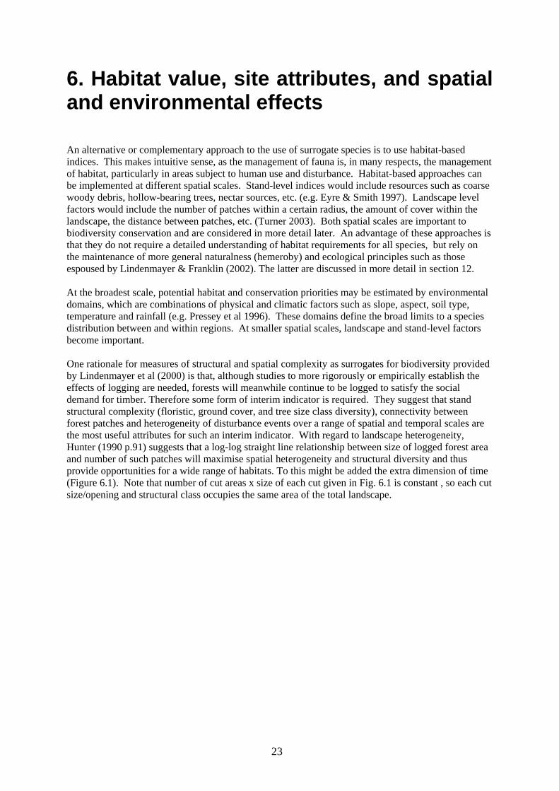
23

6. Habitat value, site attributes, and spatial and environmental effects An alternative or complementary approach to the use of surrogate species is to use habitat-based indices. This makes intuitive sense, as the management of fauna is, in many respects, the management of habitat, particularly in areas subject to human use and disturbance. Habitat-based approaches can be implemented at different spatial scales. Stand-level indices would include resources such as coarse woody debris, hollow-bearing trees, nectar sources, etc. (e.g. Eyre & Smith 1997). Landscape level factors would include the number of patches within a certain radius, the amount of cover within the landscape, the distance between patches, etc. (Turner 2003). Both spatial scales are important to biodiversity conservation and are considered in more detail later. An advantage of these approaches is that they do not require a detailed understanding of habitat requirements for all species, but rely on the maintenance of more general naturalness (hemeroby) and ecological principles such as those espoused by Lindenmayer & Franklin (2002). The latter are discussed in more detail in section 12. At the broadest scale, potential habitat and conservation priorities may be estimated by environmental domains, which are combinations of physical and climatic factors such as slope, aspect, soil type, temperature and rainfall (e.g. Pressey et al 1996). These domains define the broad limits to a species distribution between and within regions. At smaller spatial scales, landscape and stand-level factors become important. One rationale for measures of structural and spatial complexity as surrogates for biodiversity provided by Lindenmayer et al (2000) is that, although studies to more rigorously or empirically establish the effects of logging are needed, forests will meanwhile continue to be logged to satisfy the social demand for timber. Therefore some form of interim indicator is required. They suggest that stand structural complexity (floristic, ground cover, and tree size class diversity), connectivity between forest patches and heterogeneity of disturbance events over a range of spatial and temporal scales are the most useful attributes for such an interim indicator. With regard to landscape heterogeneity, Hunter (1990 p.91) suggests that a log-log straight line relationship between size of logged forest area and number of such patches will maximise spatial heterogeneity and structural diversity and thus provide opportunities for a wide range of habitats. To this might be added the extra dimension of time (Figure 6.1). Note that number of cut areas x size of each cut given in Fig. 6.1 is constant , so each cut size/opening and structural class occupies the same area of the total landscape.

24

Figure 6.1 Maximum combined spatial and structural heterogeneity in a logged landscape (after Hunter 1990)

Limitations of spatial indices include different species responses to fragmentation, lack of clear impact thresholds (Lindenmayer et al 2005), and difficulty in differentiating between fragmentation and diminished area effects per se (Cooper and Walters 2002, Fahrig 2003). For many species, (excepting dispersal-limited species), the proportion of critical habitat in the landscape is more important in maintaining populations than its degree of non-consolidation (Turner et al 2003).

McAlpine & Eyre (2000) tested a range of landscape metrics to evaluate MC&I (1.1e) ‘fragmentation of forest types in dry eucalypt forests of subtropical Queensland. Using target species of gliders (4) and diurnal birds (6) as well as measures of total bird diversity and nectar-feeding bird diversity, they found that stand structural and compositional attributes were more influential than landscape metrics with scales of influence at stand (2 ha) and various landscape (78-1250 ha) extents. However even the most influential site variables had only weakly predictive ability for counts of most species (R2 ~0.10-0.17), notwithstanding that the probability of some effect existing was significant (e.g. p<0.05). The strongest correlation (R2=0.176 p=0.000) to any landscape metric variables was that of yellow-bellied gliders (Petaurus australis) to “trace” proportions of senescent trees in the landscape within 2km from the sampling transect. The correlation of other species, including greater gliders (Petauroides volans), exudivores and diurnal birds, with traces of landscape-level remnant was also low (R2 <0.15).

Size of each cut area Time

N cuts

25

Figure 6.2 Fauna & Habitat correlation reproduced from McAlpine & Eyre 2002 On the basis of this result, McAlpine & Eyre (ibid.) claimed “We have been able to establish a strong positive relationship between the proportion of older forests and the count of yellow-bellied gliders…..[and ] …. We are able to confidently report that the amount of forest with a trace or subdominance of older trees is a reliable indicator for arboreal marsupials in these selectively logged dry eucalypt forests”. Such claims seem tendentious in view of the weakly predictive relationship of the chart. It is more reasonable to say from the evidence that senescent trees may be a necessary but not sufficient predictor of habitat occupancy. McAlpine & Eyre (ibid) also tried a logarithmic fit to their data but rejected it because of low R2. In contrast to the projected line, it is impossible to say what is likely to happen to population counts beyond the 30% landscape occupancy. In a modelling study, Fahrig (2001) found that reproductive rate was likely to be the most important factor in localised extinctions, with habitat distribution pattern having only very small effects in a matrix of high and poor-moderate quality habitat. Other life-history parameters may also be important. For example, Goldingay and Sharpe (2004) found that the adult mortality rate had the most impact on the probability of population persistence of squirrel gilders (Petaurus norfolcensis) in fragmented habitats in urban Brisbane. Both modelling studies reported the counter-intuitive finding that dispersal increased the probability of extinction. While dispersal is necessary to recolonise empty areas of habitat, this finding arose because of dispersal related mortality (Fahrig 2001; Goldingay & Sharpe 2004). Thus, Tyre et al (2001) found that modelled predictions of territory occupancy by arboreal marsupials according to assessed habitat quality could only attain about 50% accuracy at best because of stochastic demographic factors. No single indicator shows high correlation with a wide range of species (Eyre and Norman 2002) . Hence spatial features may not always have a measurably strong link with actual fauna presence or abundance. In an empirical study, Pearce and Ferrier (2001) used stepwise regressions to investigate whether broad environmental attributes (temperature, rainfall, degree and proximity of logging disturbances, soil type and lithology etc) could be used to predict abundance of vertebrate fauna and vascular plant species as recorded across more than 670 sites in northeast NSW. They found that (if non-occupied sites were excluded), neither presence-absence nor actual abundances could be reliably predicted from the environmental variables, for all but a few species. Their results suggested that “existing data sources are inadequate to provide any reliable regional models of species abundance,

26

using any of the statistical techniques examined”. However, in more highly altered landscapes, fragmentation effects or spatial patterns may become critical and/or obvious. For example Cox et al (2003) found mammal species increased with the area of “island” rainforest fragments in a cleared landscape, and that larger mammals were most likely to be absent from smaller fragments. The process of prioritising management options for ESFM principle “conservation of biological diversity and ecological integrity” can be guided by methods used for selection of reserve areas where there is a limited budget, and a range of competing potential land-use options (including resource harvesting and/or conversion to cleared land) which all have various degrees of return on investment and ecological risk. (Margules et al 1991, Faith et al 1996). Armstrong et al (2004) suggested that “in areas which are not extensively developed, much biodiversity can persist on non-reserved or “matrix” land. …[However] ..in regions dominated by agricultural and residential lands, reserves must function more like an archipelago of natural areas in an inhospitable ocean..” and formal reserve design and management are more important. Pressey et al (1996) determined conservation priority for northeast NSW forests by considering current reservation extent and vulnerability to future clearing in 81 environmental domains based on rainfall, temperature, soil fertility and slope. Steep infertile land domains were over-represented in the formal reserve system due to historical factors, and private or non-reserved land in domains where there were fewest options in space or time were considered to have highest priority for additional reservation. An objective of maximising the number of species conserved with minimum land acquisition or sacrifice is best achieved by selecting sites which are complementary in species richness, rather than targeting hot-spots of high species richness, or habitat or vegetation representativeness (Kati et al 2004). Hence indices of richness per se may be less useful than knowing the abundance and representation of species or groups of species at various sites. However, this information may be difficult and costly to obtain. From the studies cited, the implicit assumption in many cases that greater numbers of individuals equates to higher habitat quality (where quality means probability of survival and successful breeding) is highly questionable (see discussion above on source/sink dynamics). Thus, Tyre et al (2001) concluded that habitat “quality” as assessed, was an indication of the ability of animals to reach and colonise an area rather than successfully reproduce and expand in numbers. From this brief overview, it appears that neither broad environmental attributes nor spatial features are highly correlated with fauna species abundance. Logging history appears to affect probability of presence of some species, but any negative effects may be ameliorated by management of vegetation structure and the surrounding matrix. Indicator species could be used to monitor effects of harvesting on biodiversity in northeast NSW, but inferences about management effects may not be reliable because of demographic stochasticity and the lack of common trajectories between species. Long-term research would be required to overcome these limitations.

Nevertheless, a valid argument remains that, although they may not be strong predictors of actual occupancy, structural features are potentially limiting resources and, as such, are useful indicators of potential habitat. For example Catling (1991) shows that small mammal abundance was significantly (r2 >0.73 , p<0.001) correlated with increasing habitat complexity score based on vegetation structure, for NSW sites at Nadgee (south coast) Kosciousko (alpine) and Chaelundi (northeast)

Therefore, using vegetation structures as an index measure is at the least an effective and efficient means of implementing the precautionary principle, and may often be a useful and real indicator of habitat value and occupancy. Maintaining structural vegetation features seems to offer a valid rational cost- and risk-minimising approach to sustainable biodiversity management when considered in the broad temporal and spatial landscape and where the costs are fairly apportioned in relation to the benefits.

27

7. Resolving the use of fauna indicators Kavanagh et al. (2004) suggested that the monitoring of representative fauna and flora species (those for which a significant change in population was most likely to indicate changes in other species) would be important in logging areas in addition to monitoring habitat structural features. This is because the efficacy of the structure-based approach requires assessment, and possibly refinement (see below: adaptive management). Species monitoring might serve to confirm that actions are having the desired effect and may reveal where factors other than habitat availability are affecting population size, density and survival. Kavanagh et al. (2004) suggested the monitoring of species with a known sensitivity to logging. They developed species response curves that were used to identify species with similar responses (discussed in more detail below). Species sensitivity was determined from extensive data sets used in their literature review. Thus, Kavanagh et al. (2004) essentially advocate a focal species approach. However Lindenmayer et al (2000) have argued that competitive exclusion and asynchronous stochastic inter-species population dynamics limit the reliability of indicator species as a general tool for monitoring.

Kavanagh et al. (2004) assigned species to 8 categories indicating potential sensitivity to logging and developed generalised post-logging response curves for fauna populations, based essentially on expert judgment. Using the response curves and estimating potential exposure to logging, a comprehensive list of potentially affected species was developed. However the assumed response curves were based on stand-replacing events (i.e. complete felling and replacement by regeneration), and as a generalised hypothesis, excluded the potential ameliorating effects of the landscape matrix around the logged area. Therefore the logging impacts could well be considered as worst case scenarios, particularly where selective logging is practiced. Species regarded as highly sensitive to logging included epiphytes and other non-vascular plants, large owls, mistletoe feeders and large hollow-dependent birds, large hollow-dependent arboreal marsupials, and carnivorous marsupials. Sensitive fauna typically had low natural population densities, specialised diet or habitat requirements (e.g. dependence on hollow-bearing trees; preferred open midstorey), occurred at the top of the food chain, and/or exhibited a social population structure (Kavanagh, 2004). Many of these attributes also make it difficult to conduct a valid statistical assessment of population trends due to low statistical power. Kavanagh et al (2004) also investigated the correlation between species groups abundances and time since logging using retrospective (chronosequence) studies. In south-east Queensland, species richness and abundance of reptiles was highest 0-10 years after logging, while birds were similar across 5 successional stages of forest regeneration. Of 348 vertebrate species in northeast NSW assessed on 619 sites, 40 were disadvantaged by logging, 40 advantaged, 147 largely unaffected, and 121 were recorded too rarely to be able to draw conclusions. Most species were widely distributed through both logged and unlogged landscapes, and like the Pearce and Ferrier (2001) study, only presence/absence rather than abundances showed any correlation with site features. This is presumably due to the influence of factors (e.g. population dynamics, competition, predation) other than logging. These conclusions are, therefore, subject to the caveat of most chronosequences, notably the difficulty of making firm conclusion in the absence of pre-event measures on given sites, valid treatment replicates and controls monitored over the same time period. While we agree with Kavanagh et al. (2004) that the monitoring of species sensitive to logging is required to assess the efficacy of structural-based indices, we also consider the reservations of Lindenmayer et al. (2002; 2000) regarding landscape-scale measures and indicator species to be well-founded. Thus, we will incorporate a target species approach in our sustainability metric. In common with the focal species approach, the target species method involves the identification of species sensitive to logging, which are then monitored on some proportion of sites. Kavanagh et al. (2004) provide some guidance in regard to the selection of species and the design of monitoring programs; some potential pitfalls of interpretation are discussed in section 11 below. Unlike the focal species

28

approach, however, the response of the target species is only relevant to that species. Its response is not extrapolated to that of other species, which are likely to differ in some respect to that of the target species.

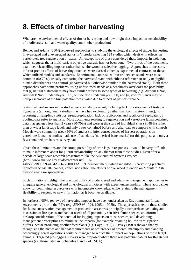
29

8. Effects of timber harvesting What are the environmental effects of timber harvesting and how might these impact on sustainability of biodiversity, soil and water quality, and timber production? Bennet and Adams (2004) reviewed approaches to studying the ecological effects of timber harvesting in even-aged and uneven-aged stands in Victoria, selecting 124 studies which dealt with effects on vertebrates, tree regeneration or water. All except five of these considered these impacts in isolation, which suggests that a multi-variate objective analysis has not been done. Two-thirds of the documents examined clearfelling impacts rather than shelterwood or selective logging. Approaches to measure, infer or predict effects of harvesting practices were classed either as experimental contrasts, or those which utilised models and standards. Experimental contrasts within or between stands were most common (60-70%), usually comparing the harvested stand with either a reference (usually negligible human disturbance) or a control (unharvested but otherwise similar to the harvested stand). Both these approaches have some problems; using undisturbed stands as a benchmark overlooks the possibility that (i) natural disturbances may have similar effects to some types of harvesting (e.g. Attiwill 1994a; Attiwill 1994b; Lindenmayer 1995, but see also Lindenmayer 1990) and (ii) control stands may be unrepresentative of the true potential forest value due to effects of past disturbance. Statistical weaknesses in the studies were widely prevalent, including lack of a statement of testable hypothesis (although many studies may have had exploratory rather than confirmatory intent), no reporting of sampling statistics, pseudoreplication, lack of replication, and sacrifice of replicates by pooling data prior to analysis. Most documents relating to regeneration and vertebrate fauna contained data that spanned less than 3 years (60-70%) and were at the scale of individual sites (81-88%) rather than at wider landscape level, and only a few contained before-and after data to compare with controls. Models were commonly used (50% of studies) to infer consequences of harvest operations on vertebrate fauna; no studies made use of standards (numerical benchmarks) for this purpose and only a few contained pre-harvest survey data. Given these limitations and the strong possibility of time lags in responses, it would be very difficult to make inferences about long-term sustainability or lack thereof from those studies. Even after a decade of large scale research programmes like the Silvicultural Systems Project (http://www.dse.vic.gov.au/dse/nrenfor.nsf/FID/-44058C2BD622F4464A25677500113A5E?OpenDocument) which included 13 harvesting practices replicated across 107 coupes, conclusions about the effects of overwood retention on Mountain Ash beyond age 8 are speculative. Such limitations highlight the practical utility of model-based and adaptive management approaches to integrate general ecological and physiological principles with expert understanding. These approaches allow for continuing resource use with incomplete knowledge, while retaining the management flexibility to respond to new information as it becomes available. In northeast NSW, reviews of harvesting impacts have been undertaken as Environmental Impact Assessments prior to the RFA (e.g. SFNSW 1994, 1995a, 1995b). The approach taken in these studies for fauna conservation management in production areas was principally a comprehensive listing and discussion of life cycles and habitat needs of all potentially sensitive fauna species, an informed desktop consideration of the potential for logging impacts on those species, and developing management prescriptions to minimise the impacts (for example retaining hollow trees, riparian buffers, nectar-producing or other feed plants [e.g. Loyn, 1985]). Davey (1989) showed that by recognising the niches and habitat requirements or preferences of arboreal marsupials and planning accordingly, forest operations could be managed to reduce their impact on populations of those target animals. Targeted pre-logging surveys were proposed where there was potential habitat for threatened species (i.e. those listed in Schedules 1 and 2 of TSCA).

30

9. Timber production indicators PNF as currently practised in northeast NSW is predominantly selective logging or small group selection in mixed age and mixed species stands. In plantations, typical minimum harvest areas or volumes are 20ha or 1000m3 respectively in order to justify costs of moving equipment , and smaller volume sales from multiple sellers usually results in lower prices received.(James 2001; McCormack et al 2000). In PNF, per hectare harvest volumes are lower as explained below. Harvests occur at intermittent periods (cutting cycles) of 10-20 years, and typically some 10% to 50% of gross standing volume may be removed over logging areas of 10-150 hectares (commercial yields 10-50m3/ha). 9.1 Sustainable silviculture: maintaining an even flow of timber One of the oldest and most basic concepts in forestry is that of “sustained yield”, which simply means that the yield of wood products, measured in the volume of merchantable tree boles, does not diminish over time. The potential productivity of a given forest type will depend on rainfall and other climate characteristics, soil type, and the genetic potential of tree species on that site. It is not easy to estimate the “non-declining sustainable yield” of a region and to express it in terms of cubic metres per hectare per year over an area of varying forest types and with forests in different stages of growth . The “natural” lifespan of a given forest, often determined by the length of time between stand-replacing fires, can be considered in determining expected annual yields and setting rotation lengths. But if the apparent natural lifespan (time to onset of senescence) for a forest type, Blackbutt for example, is two to three hundred years and average growth over time (MAI) peaks at age 30 years (at 11 m3/ha/yr) (Baur, 2001) then there would be a long period of diminishing returns if the forest developed for several hundred years. Eventually older forests have a very small or even negative level of net primary production. For these reasons timber-oriented forestry has long been practised with rotations that are “truncated”, that is reduced to the period of fairly rapid growth, perhaps ending at the period when the curves for mean annual increment (MAI) and current annual increment (CAI) coincide. This takes advantage of the period of rapid growth in the early life of a stand. Thus a forest harvested four to six times at fifty year intervals would have a much greater MAI and estimated sustainable yield than one harvested at two or three hundred years. Of course, flora and fauna that depend on later stages of growth for parts of their life cycles would be disadvantaged if the entire forest estate were put on shortened rotations. This simple example is for even-aged stand management, but the broad principles also apply in the case of stands of mixed age. Managing for productive condition by selective logging means maintaining the increment (MAI) of individual trees by careful selection of removals and retentions at harvest time according to spacing, crown vigour and site potential. Stand MAI is measured as harvest yield divided by cutting cycle period. MAI x stumpage value is thus equivalent to an agricultural Annual Gross Margin. In commercial production, a financial optimum is obtained if trees are removed when they are no longer increasing in value at the level sought by the manager. This has some strong implications for the nature of the forest’s structure, which are further discussed below. The potential sustainable yield should be based not only on good data about the average increment in all diameter classes over long periods of time, but should consider potential losses. There are many sources of loss of increment but among the major ones are fire – bushfires will inevitably take some percentage of trees or even forests over the long term, fungal decay – heart rot and sap rot are important causes of loss, and insects – herbivorous insects slow down growth and termites consume significant amounts of wood. Logging damage to residual and felled trees are also reasons why yield may be less than apparent growth.

31

Current yields and trends are included in MC&I (e.g. indicator 2.1.d Annual removal of wood products compared to the sustainable volume) but it is important to note two circumstances under which this indicator is misleading (Vanclay 1996). The first is a transition from predominantly old-growth forest structures to regrowth. In this case the accumulated volumes from a long period time in the form of large slow-growing trees, may be removed from the forest over the first one or two cutting cycles. The high harvest yield that this produces will not be repeatable at the next cutting, however the growth in the interim has been more rapid. Hence yield appears to decline in the short-term, even though it will in fact have increased. The second situation is also where there is an accumulated stock of trees, and every cutting cycle the harvest is constant or even increasing. This appears to be sustainable for the first few cycles; however if the harvest removals are greater than the growth rate, eventually the stock of trees will be reduced to those too small to harvest and the yield collapses. 9.2 Forest condition and removals; regeneration and gap size Baur (2001), in his notes on the silviculture of eleven major forest types in New South Wales, considered these categories: the virgin forest, even-aged stands and irregular stands. Further, he discussed various types of damage to older stands. Baur (2001) noted that virgin blackbutt forests, which occurred in a mosaic of even-aged patches, could have ages up to five hundred years and on high quality sites might have averaged yields (total standing volume) of 300 m3/ha, with up to 600 m3 under ideal conditions. Spotted gum stands, in contrast, tended to be uneven-aged and would have had about 300 m3 per ha of which typically a third was merchantable. In more typical non-ideal conditions , Horne & Carter (1992) reported average (gross) volumes in managed blackbutt forests immediately prior to second logging of 154m3/ha around Kendall NSW, compared to average volumes in unlogged forest of 160m3/ha. Dry sclerophyll forests, with spotted gum and ironbark as major canopy species, have a different regeneration mode. Rather than reproducing directly from seed, spotted gum forests mostly rely on a pool of lignotubers. When openings are made these lignotubers are “released” and grow into vigorous saplings. Spotted gum forests are more commonly dominated by grassy understories rather than by the thick moist vegetation of wet sclerophyll forests. Thus there is less need for disturbance by mechanical means or fire and in fact heavy fires can destroy lignotubers. But there is requirement for light: Baur (2001) suggested that the retarding effect of adjacent vegetation is such that openings of at least 30-40 meters in diameter are needed so that some trees can grow unimpeded and larger openings would be required to produce vigorous groups of regrowth. Basset & White found that suppressive effects on young regrowth may extend 70m from the edge of a logged stand or coupe, so logging areas of less than this radius (i.e. 1.5 ha ) will experience significant growth reductions compared to potential. Opening size requirements may be larger on steep south-facing slopes. Opening the stand sufficiently to promote access to light and reduce moisture competition from existing trees is also required in order to “release” regrowth and subdominants after selective harvest or overwood thinning operations. Basset & White (2001) found that regrowth volume and height growth losses can be in the order of 15-50% compared to clearfelling when 10-30% basal area is retained in “reference” stands with an initial 40m2/ha BA. The highest impacts were on lower rainfall sites or if retention comprised scattered large trees. As an example of the latter, with 5 trees per hectare of 100cm DBH comprising around 4m2/ha basal area, growth losses were estimated to be 10-40% in a “reference” stand depending on stand structure/composition at the harvest time. Various authors (Basset & White, 2001) have calculated “zones of suppressive influence” around existing overwood, of 2-6 x crown radius depending on tree vigour. Dore et al (1999) have described silvicultural practices suitable for various forest structures in northeast NSW. In regrowth forests, a typical PNF removal at each cutting cycle might be around one third of standing volume of which some 70-90% may be merchantable (internal defect is often impossible to detect while the tree is standing). Typical harvest thus removes 10-50m3/ha with a 10-20 year return period. (Reported average harvest removal for NSW public native hardwood forests is

32

60-80m3/ha between 1999 and 2003, [FNSW, 2004] ). For native forests – wet and dry sclerophyll types - in New South Wales, the range of potential productivity generally varies from ~5-30 m3/ha/yr. But the actual productivity of useable solid wood can be much lower than this in exploited forests, as little as 0.5 to 1 m3/ha/yr. (NNFS 2002). This happens because either there is very little total increment of biomass and or because the trees on which the growth is occurring have no commercial value. Since there is no local market for pulpwood, biomass or other smallwood, thinning from below (removing small trees while retaining larger ones) is rare in northeast NSW PNF, and most harvest operations tend to be a simple extraction of commercial material only, ie larger sizes. Unfortunately this usually means that the retained trees are those which are suppressed or defective. There is often little attention given to silvicultural improvement such as retention of vigorous trees and culling of suppressed, defective or non-commercial trees which occupy the potential growing space of better trees. Over time this has led in many cases to stands which are in poor silvicultural condition and can only be restored to their productive potential over a very long period of time, or by radical culling and “re-set”. In forests which have been degraded in this way the potential sustainable yield is nowhere near being attained, Combe et al. (1998) described a typical dry sclerophyll forest on private land –

* regrowth forest with an inverted J-curve uneven-aged structure, meaning many trees in the lowest diameter classes and progressively fewer as size increases, with sometimes a few very large trees. * previously subjected to several episodes of high grading, * with 85% of trees of no commercial value, and

thus a forest very much in need of rehabilitation to achieve its potential for timber production. Without adequate regeneration of desired species, or with regeneration that grows poorly, the objective of sustainable timber production cannot be achieved. This has been particularly problematic in moist (wet) sclerophyll forests. To maintain a canopy of eucalypts, these forests depend on disturbance events. To achieve good results it has been necessary to reduce canopy cover by 70%, create a high degree of disturbance on the ground, and sometimes use prescribed burns (Nicholson, 1999). This creates a suitable seedbed for germination and rapid early growth of blackbutt and other eucalypt species. Without such disturbances the understorey is often dominated by vines and other short-lived rainforest pioneer plants. Thus single tree selection and small group selection methods are not effective in achieving adequate regeneration and subsequent growth. This was well demonstrated in a series of experiments at Pine Creek SF (Florence, 1996) where “radical” treatments led to better volume increments of target species than did “conservative” treatments. SFNSW (2005) describes the 3 basic silvicultural procedures currently used in public forests. These are Single Tree Selection (STS), Australian Group Selection (AGS), and Thinning. A manual is used to assess, on a site-specific basis, the condition of the forest and formulate the appropriate silvicultural approach for regeneration (STS or AGS) or growth (thinning). The Integrated Forest Operations Approval (IFOA) specifies constraints

• STS regimes permit up to 40% of the stand basal area in the net harvestable area to be removed at harvest.

• AGS constrains canopy openings to 0.25ha (equivalent to a 57 metre diameter circle) and collectively to less than 22.5% of the net harvestable area in a single harvesting event.

• Harvesting events should be a minimum of five and an average of seven years apart. • Thinning is limited to the removal of 60% (maximum) of the basal area of the stand.

33

9.3 Economics of stand rehabilitation Combe et al. (1998) discussed the nature of dry sclerophyll forests on private lands in NSW and presented a theoretical case study of a property. They argued that such degraded stands could greatly benefit, in terms of productivity, from silvicultural treatments that eliminated many slow-growing stems and directed the growth potential of sites onto a few selected trees. Further, Jay (2005c) investigated the dynamics of mixed species uneven-aged forests in northeast NSW using stochastic modelling with the aim of determining optimum silviculture and harvest removals/retentions patterns for a range of site conditions, initial stand structures, and silviculture treatments. The mechanistic model EUCAMIX (Jay 2005c) was used which predicts tree growth in mixed and even-aged stands based on site quality, species, crown vigour and competition. EUCAMIX also incorporates regeneration and mortality responses to logging events. The EUCAMIX model was used to simulate growth and development of the most common current structure and forest types in the region: dry Spotted Gum or Blackbutt stands on average site quality with 75% of standing biomass in the regrowth size classes (<40cm DBH), ie similar to that described above by Combe et al (1998). The mean representative stand structure, described as basal area by crown vigour classes, species commerciality and timber product, is shown in Fig 9.1. Figure 9.1 A representative stand structure for mixed-age Spotted Gum forest in north-east NSW. The horizontal axis is DBH class (cm) in 15cm intervals and the vertical axis is stand basal area (m2/ha). At initial inventory, stand basal area was 24.4 m2/ha.

Timber species Crown Vigour Product Grade LowValSp Suppr Waste SecondarySp Interm Pulp HighValCommSp CoDom LQ sawlog Dom HQ sawlog

With an objective of maximising Net Present Value at 5% real discount rate of the sum of harvests plus change in standing value over a 30 year period, Jay (2005c) found that high-grading (with a modest amount of culling) was the harvest pattern most likely to maximise mean NPV. The reason for this outcome became obvious when the value of individual trees was considered (Fig 9.1). Most trees in the 30 year life of the stand ceased to increase at more than 5% value per year once their diameters exceeded 60cm DBH, regardless of species, crown vigour or stand competition. Hence to maximise NPV, a PNF landowner is acting “rationally” by high-grading if his/her discount rate (opportunity earning rate) exceeds 5%, and if the other perceived benefits of forest ownership do not offset a lower earning rate.

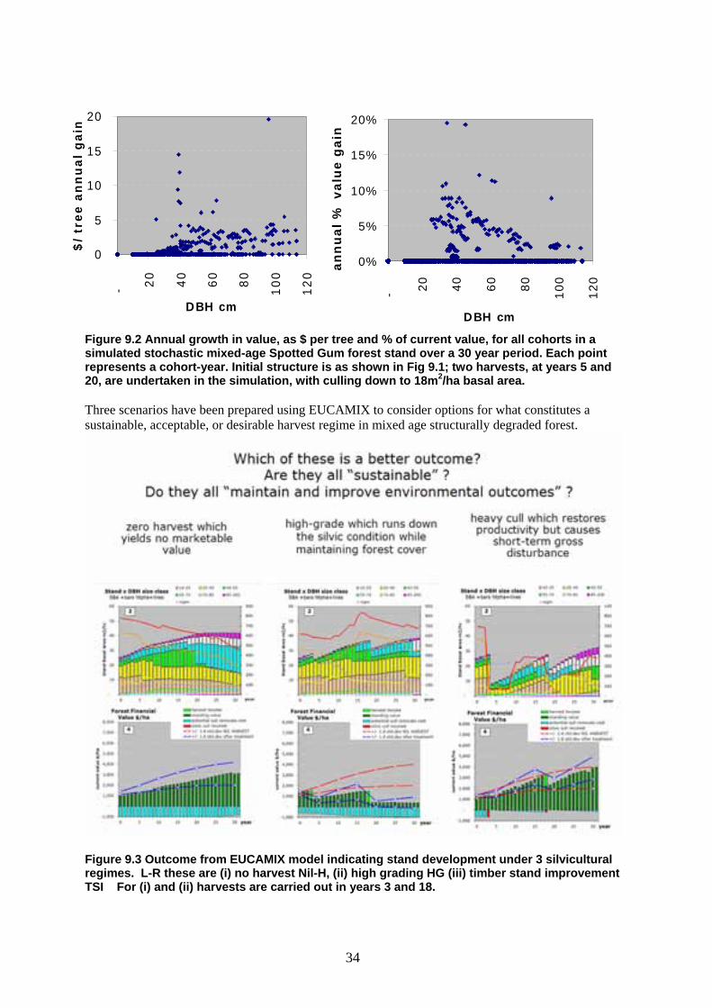
34

0

5

10

15

20- 2

0

40

60

80

100

120

DBH cm

$/

tre

e a

nn

ua

l g

ain

0%

5%

10%

15%

20%

- 20

40

60

80

100

120

DBH cm

an

nu

al

% v

alu

e g

ain

Figure 9.2 Annual growth in value, as $ per tree and % of current value, for all cohorts in a simulated stochastic mixed-age Spotted Gum forest stand over a 30 year period. Each point represents a cohort-year. Initial structure is as shown in Fig 9.1; two harvests, at years 5 and 20, are undertaken in the simulation, with culling down to 18m2/ha basal area. Three scenarios have been prepared using EUCAMIX to consider options for what constitutes a sustainable, acceptable, or desirable harvest regime in mixed age structurally degraded forest.

Figure 9.3 Outcome from EUCAMIX model indicating stand development under 3 silvicultural regimes. L-R these are (i) no harvest Nil-H, (ii) high grading HG (iii) timber stand improvement TSI For (i) and (ii) harvests are carried out in years 3 and 18.

35

In Fig 9.3 the top row of charts shows stand basal area (bars) and trees per hectare (lines) by size class, and the bottom row (bars) show standing value, including culls and harvests undertaken. The lines in the bottom row charts are ±1.0 standard deviation from the mean for current (blue) and unharvested (red) stands, and thus represent the stochastic range of potential value outcomes. Clearly stand structures are maintained in the first two treatments, since in both cases the forest basal area does not diminish below initial level over time, and the number of large trees also increases. The second option provides the greatest net cash flow, but the value of the forest is run down to almost nothing, since all valuable trees are taken out and no growing stock is left. The third treatment involves two harvests which make significant changes to stand structure. The first of these involves a period of low basal area (minimum 8m2/ha) for some time after culling, and there is also a negative net cash flow at first harvest because of the cull cost*. This was often traditionally done by ring-barking (Florence, 1996). However by retaining the more valuable stand components, the stand value is substantially increased, and within the 30 year period, there are more large trees than either of the first two options. * Cull costs in the EUCAMIX model are estimated to be 5 cents per cm of DBH, (e.g. $1.50 for a 30cm tree) which is considered to be achievable by contractor axe-poisoning. Sensitivity to cull cost has not been analysed. Note that this method means standing dead wood is retained, with opportunities for habitat value Table 9 Mean NPV outcomes ($/ha) for 3 main silvicultural treatments, with some variants involving additional retention prescription. (SE ~6-8% of mean for NPV0% values at p=0.10, n=128, SE~15-20% for NPV5%) Cull net cash flow Treatment NPV 0% NPV 5% <-$100 <-$200

1. Nil Harvest 1948 -202 2. HG (no culls) 1156 454 HG (culls to 18m2/ha) 1855 554 0 0 WithCode* HG (no culls) 1535 182 0 0 WithCode* HG (culls to 18m2/ha) 1945 239 10% 6% 3. TSI (no constraints) 4278 448 90% 5% TSI (culls to 18m2/ha) 3326 378 0 0 WithCode* TSI 2415 81 12% 1%

The charted scenarios from Fig 9.3 are Treatments numbered 1,2,3 respectively in Table 9, which shows mean NPV ($/ha) outcomes (SE ~8% at p=0.10, n=128) Additional scenarios to analyse the outcome of (i) culling to a retention limit of 18m2/ha and (ii) culling to that retention limit AND retaining 10 largest trees per ha (With Code*) are also shown. The columns at right indicate the number of times in which the stochastic stand outcomes were such that stumpage income minus cull cost is less than -$100, and -$200, ie that outlays exceeded income by those amounts in order to undertake the cull as prescribed. The additional scenarios used simple rules proposed in the draft NSW PNF Code, being post-harvest retention of 18m2/ha basal area including 10 largest trees per hectare as a proxy for hollow-bearing habitat and recruit trees. The results show that if NPV 5% is a decision criterion, then HG with some culling is optimal, confirming that current practice is “rational” from the landholder’s financial point of view. NPV at 0% was also recorded from the simulations as shown in the table. If improvement in value does not

36

take time-cost into account (NPV 0%) then not harvesting is better than High Grading, but TSI is the best of the three**. Hence with 0% discount rate, optimal silviculture treatment involved significant culling with retention of larger dominant trees. With this treatment a stand can be restored to a more balanced structure of biomass distributed across size classes within the 30 year period, notwithstanding 2 harvests occurring in that time. After two harvests, more large trees will be present than at commencement (Fig 9.3). Using NPV 5%, HG with no culls is about the same value as TSI, but undertaking TSI to the intensity required to match HG can only be undertaken if in 90% of cases, the landowner is prepared to spend more than $100/ha over and above stumpage income from a harvest undertaken at that time. Given the choice between risky future gains in return for outlays now, or risk free returns now with negligible future returns, many landowners will opt for the latter, especially if sovereign risk is added to the former. ** Jay (2005c) derives silvicultural treatments by heuristic methods that are better than this representative TSI treatment. The With Code effects of additional large tree retention, arising both from lost opportunity of sale and competitive effects on retained stand, are substantial with regard to NPV 5%, but negligible for NPV 0%. This happens because the NPV formulation includes net standing value at end of period and thus includes the value of these unharvested large trees; if these are not discounted it does not matter much to the value sum if they are left standing or harvested. The main economic effect of the Code* under High-Grading appears to be foregone sales opportunity; there is negligible value loss from competition in the regrowth and retained stand because it has almost no commercial stock remaining. The competition from retained basal area is more pronounced on the TSI treatment, since most of the retained trees have commercial value. The competition effects of retaining 10 large trees are a further substantial cost. Hence the Code has considerable economic effects* if a silvicultural improvement is desired. For the With Code situation, HG with some culling remains the optimal treatment for NPV 5%. The value of TSI under the Code is better than no harvest, provided that in 90% of cases, the landowner is prepared to spend more than $100/ha over and above stumpage income from a harvest undertaken at that time. This cull cost can be reduced by increasing the retained basal area (e.g. to 18m2/ha), but this comes at the expense of lowering the total NPV. Under the Code, the expectation of cull cost being $100 greater than stumpage receipts is about 12%; however this again can be reduced if there is no cull and higher basal area is retained, at the expense of lowering total NPV. These examples highlight the scope for market incentive or stewardship schemes to counter the imperative for high-grading. An amount of around $5 per tree per year should be sufficient to offset the opportunity cost of not harvesting large trees (Fig 8.2); the total amount of stewardship paid for large trees might be in the order of $1800 per hectare (today’s values) over 30 years for this example stand (from Table 9.1, being the difference between best option No Code and best option With Code). A foreseeable outcome from the adoption of the draft PNF Code as a regulatory policy instrument is both reduced harvesting rates because of costs increases, and an accelerated degrade of timber production capacity. This will arise because landowners operating in accordance with tree retention prescriptions will be likely to seek maximum harvestable yield from their current forest without regard to future silvicultural productivity, since their expected rights to future harvest are perceived to be both eroded and uncertain. The most-affected landowners are those who have deliberately and willingly retained forest which continues to have high inherent environmental values notwithstanding a history of multiple harvests.

37

*This refers to stand level effects on yield only; it should be noted that additional costs are likely to arise from planning requirements and field operating difficulties. In 2003, SF NSW spent $6.04M on harvesting supervision and environmental compliance in harvesting 45,000 ha of native forest and 12,800 ha of softwood plantation. If the relative costs are weighted toward the hardwood by apportioning the total 50:8, this makes an average of $115 per ha (SFNSW 2005) or some $3450 for a 30 ha logging area.

38

10. Soil and hydrological processes “There is a deeply rooted and erroneous popular myth that trees make it rain and that cutting them causes drastic alternations between drought and flood. The water that falls from the sky comes mostly from air that has been moistened over warm oceans and is lifted by convection over warm surfaces or over mountain and cold air masses. Transpiration from forests by itself rarely, if ever, moistens air masses enough to make it rain. Forests are an effect of abundant precipitation rather than the cause of it. In the vast majority of cases, the cutting of living trees, by reducing losses of water to transpiration and interception, actually increases the amount of water that reaches streams. The myth probably originated from the observation that true deforestation associated with agriculture or grazing often causes rain to run off so quickly from compact soils that streams flood and then dry up.”

Smith (1997) 10.1 The role and function of stream buffers One of the most contentious issues in developing a code for private native forestry has been in defining the width of riparian buffer strips. These “no-go” areas for tree harvesting are assumed to be critical areas for conserving soils and assuring adequate water quantity and quality. But they are also some of the most productive for tree growth – thus the conflict. Stream buffers or filter strips are required in all public forest harvest operations in Australia in order to protect water quality and quantity and provide areas of undisturbed habitat. Their effectiveness in sediment control, particularly when coupled with adequate post-logging soil erosion mitigation measures has been reported for NSW (Walsh and Lacey 2003). In timber production forests, unsealed forest roads with inadequate near-stream capture or diversion are the major source of sediment and turbidity rather than the operations zone (Croke 1999 cited by Walsh and Lacey 2003, Croke 1997 cited by Chikumbo et al 2000). Riparian vegetation is an integral component of the health of river systems and a number of key ecosystem functions. Ridgway (1999) describes these functions and their relevance in the major watershed of the study area, the Clarence Valley. Riparian vegetation (and zones) ……..

• protect water quality by filtering of runoff water moving across the soil surface, as well as intercepting lateral sub-surface water moving through the soil to the river. Grassy zones are particularly effective at reducing sediment (e.g. Sheridan et al 1999, Prosser et al 2002).

• reduce turbidity by protecting against erosion and acting as traps for debris in surface flows and can maintain bank stability.

• often has higher species diversity (Lynch and Catterall 2002a), but this is not always the case. For example Hancock et al (1997) found that upland vegetation communities in Western Australia had higher species richness albeit lower structural complexity than riparian forests and communities.

• are often more productive (e.g. greater Net Primary Production [NPP] through reduced moisture stress) but this can mean less streamflow and runoff in low rainfall zones. For example Scott (1999) found in a paired catchment study in South Africa, that first year flow increases from clearing of tall woody vegetation in the riparian zone ranged from 55 to 110 mm (9-44%) per 10% of catchment cleared. In the same catchments, clearing of similar vegetation in upslope (non-riparian positions) led to flow increases ranging from 27 to 35 mm (2.5-14%) per 10% of catchment cleared. This conforms with the finding by Bren (1980) that riparian zones near Myrtleford Victoria are the source of most storm flow production.

• are important as wildlife corridors and in maintaining biodiversity (Lynch and Catterall 2002a), even as linear remnants in fragmented landscape (Bentley and Catterall 1997).

39

There is little hard data on the effectiveness of different corridor widths as terrestrial wildlife habitat (Lynch and Catterall 2002b, Catterall 1993), although it has been noted that edge effects become relatively more important in narrow linear buffers (Bren 1995, Ridgway 1999). Several authors have noted that few data are available to indicate effectiveness of corridors for species conservation; nevertheless they are widely considered to be important (Tanton 1995, p.66). Much of the information used to guide Australian riparian zone management is derived from studies in other countries (Lynch and Catterall 2002a). Studies of the habitat value of riparian and other linear corridors in NSW have focussed on the south-east forests where harvesting practices are more intensive, forest age/size structures more uniform, and ecological differences between ridge and gully vegetation more distinct, than is the case in many of the timber production forests of coastal and montane subtropical NSW. Tanton (1995 p.65), cites a number of studies which have shown that in south-east NSW, riparian zones are richer in terrestrial, avian and in-stream fauna species. In UNE NSW the distinction between moist forests and dry forests may be more important than riparian and non-riparian per se (e.g. Fanning 1995). Tanton 1995 (p.389) considered that (riparian) filter strips and other measures such as retention of unlogged areas and some trees in logged coupes, and maintenance of a mosaic of different post-burn ages, should ensure the continued occurrence of populations of most (fauna) species in timber production forests in the Tenterfield SF management area. CIE and CSIRO (2000) report that .. “Mackenzie and Hairsine (1996) compared the spatial distribution of flow and flow velocities for two separate buffers (grass filter strips and near natural riparian forests) in the catchment of the Tarago Reservoir, Victoria. From their study they concluded that:

A grass filter strip has been shown to result in slower, more uniform overland flow in comparison with a surface formed under a riparian native forest (p. 211).

More detailed results are provided by Hairsine (1996) from a similar study in the same catchment:

Dense grass filter strips were found to have sediment trapping efficiencies of greater than 95% for a relatively high intensity sediment source. These results were relatively high compared with other studies. This was attributed to the high input load and the dense and near-uniform nature of the grass in the strip. Near-natural riparian forest, predominantly litter with sparse understorey shrubs and woody debris, was found to have trapping efficiencies greater than 90% for a range of sediment-laden inflows. The sediment trapping efficiencies of both buffer types were found to diminish slightly with increasing water flow, though the results support the overall effectiveness of these buffers as measures to lessen the downstream impact of intense land use (p. 206).”

Bren (1995, 1997, 1998, 2000) conducted a series of studies based in the 6600 ha mountainous forested watershed of the Tarago river in eastern Victoria. The forest comprises mostly high quality 1939 E. regnans regrowth with some more open E. sieberi on slopes and spurs. The area has high rainfall of 1400mm p.a., and slopes >300 are common. Bren (2000) showed that the fractal dimension and drainage density of the site was representative of large watersheds in humid climates generally. Bren’s 1995 study found that the area of land occupied by buffers increased substantially with increasing width of buffers, with 95% of the catchment occupied by buffers of 300 m width. As buffer width increased to 100 m, many areas became entrapped by buffers and hence became effectively inaccessible. Individual boundaries reached their greatest complexity (fractal dimension of major stream reaches) at 10 m buffer width. In 1997 he generated 40 random hypothetical logging coupes in the catchment with stream buffers of variable width, and examined the effects on harvestable volume and value. Typically 50% of the loggable land area was removed by a 90m buffer, with a slight tendency for greater volumes to be located near the watercourses. The relationship between buffer width ‘w’ and percentage of total area occupied by buffers ‘Y’ was found to be Y = -0.489+0.65w-0.0001w2 . Thus a 16.5m buffer reduced available area by about 10%. The main effects of increasing

40

buffer width were reduced area, marginal reduction in resource quality and value, and increased complexity of operations. In 1998 Bren devised a buffer-loading measure, defined as the contributing watershed area per unit area of buffer. He found that the loading on fixed width buffers was both highly variable and independent of the Strahler order of the stream. He concluded that the rationale for having larger buffers on larger streams was not justified, at least for hydrological reasons. An alternative design criteria of keeping the buffer-loading measure constant led to defined buffers which were highly asymmetric, discontinuous and non-intuitive. The buffers defined reflected the topography, and were strongly influenced by small facets close to the stream. Under the loading criteria, buffers should be wider at stream heads and narrower elsewhere when compared to buffers of constant width. In 2000 Bren used a combination of specific area and slope index as an alternative surrogate measure for hydrologic loading, and found that if buffer widths were to be made proportional to loading, then most buffer protection would be allocated to flow convergence zones whereas other areas hardly required protection. The method was highly sensitive to loading values in individual sub-catchments and may not be amenable to field implementation because of the difficulty of assessing loading in-field and complicated tree-marking. The conclusion drawn was that, like the contributing watershed method, the convergent (high flow concentration) areas in headwaters were generally under-protected and divergent (low flow concentration) areas were over-protected in relation to fixed width buffers. Bren’s conclusions contrast with the provisions in the proposed draft NSW Code of Practice for PNF, in which there is an increasing buffer width according to Strahler order as follows.

Stream Order diagram Buffer width (m)

Stream each side of Order water course banks

1 10 2 20 3 30 4 40

Stream order is a simple method of classifying stream segments based on the number of tributaries upstream. An nth order stream is located downstream of the confluence of two (n-1)th order streams. However the rationale for the proposed Code provision appears to have been for wildlife corridor functions rather than hydrologic purposes (R. Dyason pers. comm. 2004) notwithstanding the absence of any hard evidence to support the effectiveness for this purpose. The dEOAM requires separate consideration of Threatened Species, irrespective of any stream buffer retentions. “Current studies investigating the variation in water quality between harvested and unharvested areas suggest that in native forests there is a slight but hardly noticeable difference between the two areas, which might last up to 6 months before steadily returning to pre-harvest conditions” (FNSW 2005). Carlyle et al (2003) similarly found no significant difference in N, P, and turbidity in calibrated, paired sandy catchments with ephemeral streams in the year following harvesting of an exotic pine plantation in southeast Queensland. The harvest treatment included 80 ha clearfell, and 250 ha of thinning reducing stocking in 25 year old stands from 1100 to 700 t/ha in a 900 ha catchment. Immediately after the clearfell, the area was prepared and a second rotation pine crop planted. Normal contractor procedures were employed, except that the harvest operation was concentrated into one year where it would normally have run over several, in order to avoid confounding effects of season and harvest. The post-harvest period experienced major storms and flooding, including a three-day 300mm single fall. The absence of differences thus followed what might be considered a worst-case site disturbance scenario. Turner et al (2003) cite other studies in which “It was found that the combined impacts of

41

thinning and fertilization were generally minor on a range of water quality and stream chemistry parameters and within the range of historic variation……and….Removing about 50% of crown cover by thinning the plantation (46 ha catchment fully planted with 17 y.o. pine), however, resulted in a significant reduction in water use [about 1Ml/ha/yr in a 900mm rainfall zone] in the year after treatment.” Water quantity or flow regimes (stream flow annual and periodic quantities, and runoff response to rainfall events) may be more affected by afforestation or harvesting than is water quality. Thinning of forests, or selective or small group harvest, is likely to have detectable short-medium term effects on flow regimes in small (<50ha) catchments if more than 20% of land area or trees are involved. Differences between pastured and forested catchment runoff are undetectable if rainfall is <500mm per annum, but may be around 2Ml/ha (200mm equiv) on pastured land when rainfall is 1500mm/ann; effects are greatest in relation to high and low flows (drought or storm events). It is difficult to detect an impact on streamflow after afforestation or clearing when less than 20% of the catchment is affected. Trees planted highest in the landscape have a smaller effect than those planted close to streams. Most research has focussed on smaller catchments, and extrapolating the results to larger catchments may introduce bias since spatial and temporal rainfall distribution, vegetation cover effects and proportion of catchment contributing to streamflow in any given set of events are highly variable. (Keenan et al 2004)

10.2 Area of stream buffers in UNE NSW PNF Jay (2005c) examined the marginal effects of the proposed draft PNF Code on land area available for PNF, excluding State Protected Land, (i.e. prescribed streams and land >180 slope) where buffers already apply, and also excluding land of low site quality where PNF was unlikely to be undertaken. Applying these exclusions and using GIS analyses, Jay (2005c)found that some 11.6% or 67,251 ha of the net productive PNF area is in stream buffers in UNE NSW. In the public forests “11.3% of State Forest is managed to protect water catchments”; however some of this includes Catchment Protection management priority zonings and wetland areas (SF NSW 2004). To assess the effects of possible changes in buffer widths, Jay (2005c) found that a simple multiple (e.g. halving or doubling) of width will lead to a near exact corresponding change in area affected. (nb a linear change at these widths, in contrast to Brens’ (op cit.) finding of a 2nd degree polynomial function of Buffers Area and Width ) Effects vary between forest types. As might be expected, Flooded Gum (Eucalyptus grandis) and Brush Box (Lophostemon confertus) types have the highest proportion of total occurrence in buffer zones, however their actual area is small . The largest areas affected, dry Spotted Gum (Corymbia maculata and C. henryi) types and dry sclerophyll and woodlands (various species) are near the average in terms of % reduction of available area. Jay (2005c) found that more than a third (36%) of the gross area of buffers on all forest comes from the 10m zone around Strahler 1 streams. If Bren’s (2000) scheme of buffer width according to hydrologic loading were to be used, buffers at the confluence of Strahler 1 streams would be wider than 10m, but the total area under buffers, especially on higher order streams, would be substantially less. Strahler 4 buffers comprised 24% of the total gross buffer area, although only half of this area is an effect of the Code since 20m buffers are already required on most of these streams under the “prescribed stream” provisions. The buffers are distributed across all site qualities (SQ). Although there was a clear trend for greater % reduction in available area with increasing SQ, this had little consequence in absolute hectares since the amount of high SQ PNF land is small. This minimal effect of SQ x area interaction is somewhat surprising, and may reflect the lack of detail available in the GIS system for both soil fertility (200m pixels) and topographic position (25m pixels). These resolutions may not fully capture the riparian moisture and fertility effects. Details of buffer zone area analysis by are in the accompanying report by Jay (2005b)

42

10.3 Soil management Erosion control and mitigation procedures have long been in place for harvesting in public forests (Walsh and Lacey 2003). These cover snig track and log dump rehabilitation, siting of road cross-drains and creek crossings, and use of harvest debris in sediment traps and for avoiding compaction. Ryan et al (1998) specified methods for assessing erosion hazard. Four levels of hazard are based on a combination of slope gradient, rainfall erosivity, and soil regolith stability. A similar set of approaches to hazard assessment and mitigation is adopted in the draft PNF Code. Prescribed roading standards are also included in the draft PNF Code. Some of these appear to be more stringently specified than is commonly observed as maintenance practice on public roads. eg “…Regular monitoring and maintenance of roads must be undertaken to ensure that road surfaces remain stable and drainage systems and sediment controls remain functional. …. Soil exposure on road verges must be kept to a minimum…. Drainage structures must divert water onto a stable surface, and must be kept free of debris that may impede flow of water…..” Prescriptions in this form do not add anything further to legal protection for off-site effects, since it is already an offence in NSW to cause water pollution, which is comprehensively defined under POEOA 1997. However in the form of guidelines rather than codified legal prescriptions, the standards would serve a useful advisory function. Lacey et al (2003) examined the on-site effects of forest harvesting on soil physical properties, and developed and evaluated soil indicators of SFM for southeastern Australia. They aimed to obtain and analyse data to empirically demonstrate links between degree of soil change and degree of individual and stand level growth impacts. In a logging study in SE NSW, pre-harvest measurements were made of bulk density and aeration porosity and strength (penetration resistance), on pale infertile coarse sandy soils supporting dry sclerophyll forest. Logging machine movements were mapped by GPS to ascertain traffic intensity, which was then subsequently mapped and correlated with measures of post-harvest compaction. Post-logging regeneration success and tree growth rates were also measured in 104 plots across 8 disturbance classes. The authors found about 20% of the coupe was occupied by snig tracks and other disturbed/exposed soil. Heavily disturbed classes including access tracks, log landings and disturbed subsoil accounted for a quarter to a half of all disturbance area. 80% of mapped disturbance was subject to less than 30 machinery passes, 50% had less than 10. Only the most heavily disturbed classes showed significant compaction. Other than these sites, traffic intensity (number of passes) was not clearly related to compaction. Only one site exceeded the standard of more than 20% increase in bulk density. Strong evidence of reduced growth on the heavily disturbed areas was noted, although not able to be clearly demonstrated by empirical data; a significant relationship was found only between aspect and tree growth. Some evidence of an edge effect (growth boost in trees adjoining tracks) was also noted; it was hypothesized that this may be due to reduced competition to trees adjoining the low-growth track sites. Insufficient data was available to define the effects of pre-logging soil moisture status. The high cost of directly monitoring soil physical properties was noted by Lacey et al (2003). The study concluded by recommending an indicator based on simple mapping of disturbance categories, noting this can be done efficiently only with GPS records linked to a GIS. They noted this was an interim indicator since relationships between some practices and growth outcomes were not well established, but suggested the mapping be done for a random 20% of coupes in a logging area until better information was available to quantify confidence limits. Other studies cited by Turner et al (2003) found high natural variation in soil bulk density when site is stratified based on proximity to drainage lines, lesser area of disturbances (e.g. 8% in snig tracks) than those cited above, and that estimated productivity loss 17-23 years after harvesting was 2-3%. Sampling processes were noted as difficult due to understorey thickness.

43

11. Uncertainty and risk management Risk and uncertainty need to be considered in the analysis of forestry management decisions. In the short term, sampling errors may be the major source of uncertainty, but structural uncertainty in models (i.e. knowing which variables have most influence on the outcome, and why) may be more important over the longer term. Risk describes a situation where the probability of each state of nature occurring is known, as are the consequences of that state. Uncertainty on the other hand is essentially a lack of information on either the states or their consequences, which may arise through ignorance or variability. Concepts such as biodiversity, scenic amenity, sustainability, equity or forest health are all inherently subject to uncertainty. This is because they are imprecise or even vague by definition and include information about peoples’ preferences and beliefs. The “precautionary principle” is invoked as means of rational decision-making when there is an interaction between irreversibility and uncertainty. The principle states that where there is reasonable suspicion of irreversible and significant damage, a lack of scientific certainty should not be used a prime reason for postponing preventative action. In essence it imposes a burden of proof on proponents of actions which involve risk, similar to the burden of proof in law which requires that guilt (not innocence) be proven beyond reasonable doubt. However it is often overlooked that the costs and benefits of alternative actions and their consequences can and should be quantified by risk-weighting of the outcomes. Arrow & Fisher (1974) demonstrated that, in a choice between development and preservation, if the benefits of development are uncertain and its effects are irreversible, then depending on the relative magnitude of benefits of development or preservation now and of relative costs and benefits of development now or later, it may be better to wait until more information is available before committing to development now. However one can flip this argument around. If the choice is between continued forest harvesting or cessation for preservation which has both uncertain or marginally small environmental benefits, and effectively irreversible social or economic outcomes (e.g. a loss of some critical amount of timber harvest which may make local industry unviable, or lack of silvicultural investment which may prevent a return to productive forest condition for a long period of time), then the reasoning still applies but with the choices reversed. That is to say, there are instances where the certain benefits of development may outweigh the uncertain benefits of preservation. This does not negate the precautionary principle since the essential feature is that “the expected benefits of an irreversible decision should be adjusted to reflect the loss of options this entails” (ibid), whether those options are on the development or preservation side of the ledger. Hence statistical reliability of indicators is an important issue. Measuring trends in sustainability with empirical certainty will be costly, depending on level of certainty required. There are clearly situations where trend data is not required to make a rational economic decision. For example, where the negative consequence of change (e.g. decline in koala populations around Coffs Harbour NSW, Field et al 2004) are severe, management actions may be justified without requiring certainty of decline before acting (assuming of course that we know what is causing the suspected decline and what management actions will be successful to overcome it). Nevertheless looking for evidence of change is the primary task of assessing sustainability, and in most cases this evidence is of limited certainty. How certain can we be that a damaging trend is occurring and that the consequences of the change are of sufficient magnitude to warrant action? While risk and uncertainty are inherent in ecological data and should be given consideration in index measures, what constitutes acceptable uncertainty is not always considered. Complex non-linear ecological systems are usually strongly influenced by stochasticity, and available information about the way that these systems function is often equivocal. Bringing ecological understanding into the policy arena means distilling complex analyses that predict uncertain outcomes into simple and clear advice. This creates a dilemma; should the situation be

44

simplified in a way that is persuasive but not sufficiently attendant to reliability of the conclusions; or should the uncertainties be emphasized? Harwood and Stokes 2003 suggest that “ The first option is likely to result in the caveats associated with the advice being ignored, the second is likely to result in the advice itself being ignored. Even if the advice is accepted, a high degree of uncertainty about the potential outcomes of management actions provides many opportunities for confrontation among different interest groups, and this can hinder the development of consensus.” Although these authors were discussing fisheries, the conclusions are equally relevant to forestry practices. Kangas & Kangas (2004) discuss some ways of handling uncertainties in the non-timber variables which are increasingly being given weight in forest management planning. Methods include Linear Programming in a probabilistic or fuzzy framework, heuristics using data produced by stochastic simulation, and multi-criteria analysis in a probabilistic framework. Too obtain meaningful results from these types of analyses, the statistical power of the assumed trends or changes to resource value must be critically assessed. Di Stefano (2001) provides an overview of the topic of statistical power in the context of sustainable forestry, and an example of how this is useful and relevant. Statistical power is the probability that a null hypothesis has been falsely rejected, ie a Type II error has occurred. Inductive science using classical statistics typically uses numerical data to try to disprove a null hypothesis of the form “A and B are the same”. (Ho: A=B, or A-B=0). A common assumption is that if we cannot be at least 95% sure, then the hypothesis can be safely rejected, otherwise it is accepted. However since the data is a sample, there is always a chance (5%) that the hypothesis should not have been rejected (Type I error or a “false alarm”), or that the statistical test of the samples shows a non-significant difference but a real difference in fact exists (Type II error or “false sense of security”) (Burgman et al. 1998). The probability of a Type II error occurring is large if the number of samples is small, variance is high, or the effect size is not great. This tends to be the case for many of the observations that might be made in relation to forest sustainability assessment. Type II errors are of concern in sustainable forest management since the consequence of not detecting a real difference which arises as a result of management treatments (in fauna populations, in water quality, in timber yield) may be a very large rectification cost or irremediable and regrettable loss by the time it is more certainly known. Di Stefano (2001) used a hypothetical example of a test to determine whether logging activity is causing an unacceptable decline in wildlife populations in two different locations. He calculated that 258 samples would be required in areas where changes in wildlife abundance had major economic consequences and cessation of harvesting had little economic consequence, but that only 74 samples were needed where cessation of harvesting had larger economic consequences than reduction in wildlife. The reason that a lesser number of samples could answer the same question was because the wildlife samples had a high variance and the harvesting effect was not large (i.e. typical of Type II error effects as indicated above), and the same economic consequences would arise in each situation if a wrong “snapshot estimate” of the trends in wildlife (or any similar sustainability indicator) arose simply due to stochastic factors. Hence Di Stefano (2001), (and preceding him Burgman et al.1998) proposed that conventional (but arbitrary) levels for Type I errors (e.g. α=0.05) and Type II errors (e.g. β=0.2) be discarded and replaced with the ratio α:β. The relative weighting given to the two should reflect the importance of avoiding each type of error. The confidence limits can be calculated for a given number of samples; if the sample number required to meet the desired precision exceeds the research budget then the confidence limits must be reduced. By specifying the ratio to be constant, the (economic or other) consequence of making either Type I or Type II errors increases equally. This is a means of determining the necessary trade-off between certainty, error cost and sample numbers. The most efficient sampling program, (the optimal level of uncertainty), is when the marginal costs of an extra sample is equal to the decrease in expected value or risk weighted error from the additional information that the sample provides. Burgman et al (2003) point out that this is the most scientifically credible way of implementing the precautionary principle. If monitoring programs do not have sufficient statistical power, then there is an almost guaranteed certainty that some will be failing to detect important harmful ecosystem

45

changes (false sense of security) while other are misleadingly suggesting that changes have occurred when in fact they have not (false alarm) . In the former case, when the changes become visibly apparent at some later time, the whole monitoring process can be thrown into disrepute and spurious notions of causation may be raised in future argument on the basis that past changes had not been detected. This is a social threat to the continuation of genuinely ecologically robust management systems, created by not adequately considering uncertainty. In the latter case the return to a more beneficial ecosystem condition following cessation of the activity or costly adjustments to management will be wrongly attributed to those changes. This is an economic efficiency threat to the continuation of genuinely ecologically robust management systems, created by not adequately considering uncertainty. Stochastic modelling based on mechanistic population or process models can be a means of estimating “most likely” outcomes while empirical data is limited, and thus reduce the chance of making costly mistakes. This has been used for arboreal marsupial occupancy (Tyre et al 2001), Squirrel Glider extinction probability (Goldingay and Sharpe 2004), fisheries management (Harwood and Stokes 2003), and mixed forest stand development ( Jay 2005c). Another example of sustainability planning at a regional scale is Turner et al’s (2002) use of a heuristic process to optimise forest coupe harvesting order in SE NSW, according to multiple criteria of timber production, water quality and quantity, and habitat goals. Such modelling procedures allow efficient forward estimation of management options and their risk-weighted consequences, provided that the variance and means of model outputs imitate outcomes from real datasets.

46

12. A comparison of three structural and landscape indices for biodiversity value and sustainability Since ESFM includes maintenance of biodiversity, some means of measuring biodiversity must be developed. A number of different indices and standards have been developed which use geographical position, vegetation cover and structure, and site context in the landscape as surrogates for habitat quality and importance and thus as measures of potential biodiversity. In the light of the previously described uncertainties, such indices may be seen as interim means of (i) monitoring at reasonable cost, and (ii) implementing the precautionary principle, rather than as validated empirical predictors or measures of sustainability. Indicators can be used for tracking results, exploration, and policy and other decision making. Multi-scaled indicator scores of environmental variables have been proposed as alternatives or complementary to indicators of process such as Australian Forestry Standard and the Montreal Process Criteria and Indicators for ESFM Lindenmayer & Franklin (2003 pp.96 &ff) proposed 5 general principles for sustainable management of the forest matrix,

• Maintenance of connectivity, • Maintenance of landscape heterogeneity, • Maintenance of stand complexity, • Maintenance of intact aquatic ecosystems, • Risk-spreading (for example varying the size of logging areas and intensity of activity;

Hunter, 1990 p.86 ff.) Lindenmayer & Franklin (2003 pp.96 &ff) also suggested the following should be incorporated in a checklist of stand-level indicators…

• Retention of structures and organisms at time of harvest (e.g. nest trees, coarse woody debris, understorey islands)

• Creation of structural complexity through stand management activities • Lengthened rotation times ( in uneven-aged selective logging management this might be

interpreted as an increase in diameter for allowable individual tree harvests). By inference, useful indicators are those which include ways of measuring implementation of these principles. Such indicators are commonly based on vegetation structural attributes and complexity since these are thought to be closely correlated with faunal habitat values and biodiversity (McElhinny 2002, Lindenmayer et al, 2000,) and the structural attributes are more straightforward and stable to use in practice than directly measuring and monitoring biodiversity per se. Since they are a proxy for biodiversity, measuring the status of such indicators over time following a disturbance is a means of assessing whether the disturbance causes a permanent or long term deterioration of the site (i.e. unsustainable management) , or conversely whether the ecosystem can recover quickly to a state of similar total combined attribute site value (albeit different components comprising that value) which is equal to or greater than the site value prior to the disturbance, and therefore whether the ecosystem is resilient to further such changes (i.e. sustainable management). Failing and Gregory (2003) noted 10 common mistakes when designing biodiversity indicators as a means of making better forest management decisions. They adopted a decision-oriented and risk management perspective and described these mistakes as follows.

• Failing to define endpoints, leading to monitoring of irrelevant attributes

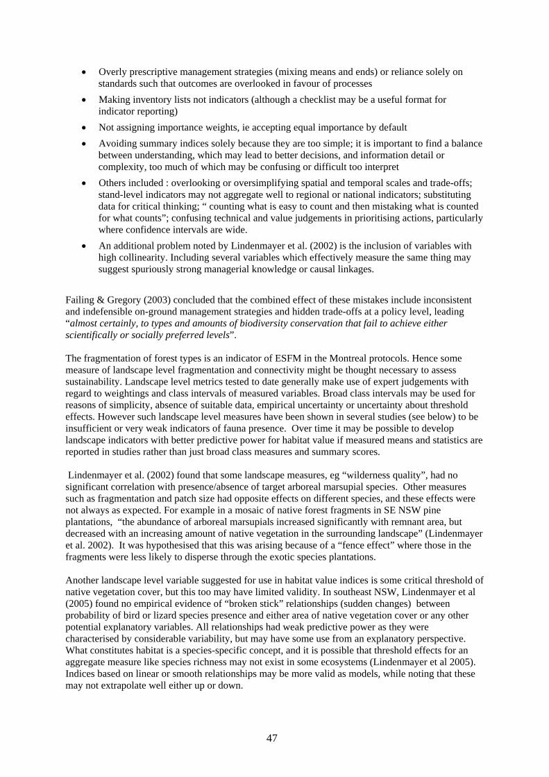
47

• Overly prescriptive management strategies (mixing means and ends) or reliance solely on standards such that outcomes are overlooked in favour of processes

• Making inventory lists not indicators (although a checklist may be a useful format for indicator reporting)

• Not assigning importance weights, ie accepting equal importance by default • Avoiding summary indices solely because they are too simple; it is important to find a balance

between understanding, which may lead to better decisions, and information detail or complexity, too much of which may be confusing or difficult too interpret

• Others included : overlooking or oversimplifying spatial and temporal scales and trade-offs; stand-level indicators may not aggregate well to regional or national indicators; substituting data for critical thinking; “ counting what is easy to count and then mistaking what is counted for what counts”; confusing technical and value judgements in prioritising actions, particularly where confidence intervals are wide.

• An additional problem noted by Lindenmayer et al. (2002) is the inclusion of variables with high collinearity. Including several variables which effectively measure the same thing may suggest spuriously strong managerial knowledge or causal linkages.

Failing & Gregory (2003) concluded that the combined effect of these mistakes include inconsistent and indefensible on-ground management strategies and hidden trade-offs at a policy level, leading “almost certainly, to types and amounts of biodiversity conservation that fail to achieve either scientifically or socially preferred levels”. The fragmentation of forest types is an indicator of ESFM in the Montreal protocols. Hence some measure of landscape level fragmentation and connectivity might be thought necessary to assess sustainability. Landscape level metrics tested to date generally make use of expert judgements with regard to weightings and class intervals of measured variables. Broad class intervals may be used for reasons of simplicity, absence of suitable data, empirical uncertainty or uncertainty about threshold effects. However such landscape level measures have been shown in several studies (see below) to be insufficient or very weak indicators of fauna presence. Over time it may be possible to develop landscape indicators with better predictive power for habitat value if measured means and statistics are reported in studies rather than just broad class measures and summary scores. Lindenmayer et al. (2002) found that some landscape measures, eg “wilderness quality”, had no significant correlation with presence/absence of target arboreal marsupial species. Other measures such as fragmentation and patch size had opposite effects on different species, and these effects were not always as expected. For example in a mosaic of native forest fragments in SE NSW pine plantations, “the abundance of arboreal marsupials increased significantly with remnant area, but decreased with an increasing amount of native vegetation in the surrounding landscape” (Lindenmayer et al. 2002). It was hypothesised that this was arising because of a “fence effect” where those in the fragments were less likely to disperse through the exotic species plantations. Another landscape level variable suggested for use in habitat value indices is some critical threshold of native vegetation cover, but this too may have limited validity. In southeast NSW, Lindenmayer et al (2005) found no empirical evidence of “broken stick” relationships (sudden changes) between probability of bird or lizard species presence and either area of native vegetation cover or any other potential explanatory variables. All relationships had weak predictive power as they were characterised by considerable variability, but may have some use from an explanatory perspective. What constitutes habitat is a species-specific concept, and it is possible that threshold effects for an aggregate measure like species richness may not exist in some ecosystems (Lindenmayer et al 2005). Indices based on linear or smooth relationships may be more valid as models, while noting that these may not extrapolate well either up or down.

48

A review of Australian studies undertaken to assess the relationship between forest fauna abundance and patterns of fragmentation (Eyre & Norman 2003) found that there was a diversity of target species responses to the various metrics considered, and that relationships between species abundances and landscape level metrics were generally weak. This result suggested a need for management regimes that promote structural diversity within the stand as well as across the landscape. Lindenmayer et al. (2000) suggested that vegetation structure based indicators which include some measure of complexity, connectivity and heterogeneity were more suitable as indicators than indicator fauna species approaches. The balance of this section is a description and comparison of 3 ways in which forest condition and processes have been condensed to a single number or small array of scores, for the purpose of assessing change over time or comparing between locations. 12.1. The Habitat Hectares (HHa) approach ‘Habitat hectares’ (Parkes et al 2003) [HHa], is an example of the form a relatively straightforward and readily applied biodiversity indicator or metric may take. HHa combines weighted site and landscape context measures into a single index which represents quality-adjusted area of habitat. To derive the HHa score, explicit comparisons are made between existing vegetation features and ‘benchmarks’ which represent the average characteristics of mature “natural” or “undisturbed” stands of the same community type. The scoring system was developed for comparative land-use decision-making and designed to be implementable by local government planners who may have not have ready access to ecological specialists. Primary aims included having an objective, consistent, repeatable measure. HHa is an example of a landscape surrogate approach. Surrogate measures are only valid to the extent that results are concordant with those that would be obtained from direct measures. Parkes et al (2003) acknowledge the approach to be a “broad-brush” (or coarse filter), rather than a definitive statement on conservation status or habitat suitability for individual species. The habitat score for a site is comprised of 7 site and 3 landscape variables, adding to 100. Weightings, or maximum attainable values for the components are… Site: large trees 10, canopy cover 5, understorey strata 25, lack of weeds 15, recruitment

10, organic litter 10, logs 5 Landscape : patch size 10, neighbourhood 10, distance to core area 5 McCarthy et al (2004) supported the move towards a explicit quantitative method with transparent and repeatable assessments compared to subjective and inconsistent judgements. However they criticised some aspects of the HHa approach, as follows:

• Inadequate connectivity measure (distance to core area) • Use of large trees as surrogate for hollows • Errors associated with visual assessment (e.g. weed cover) • Arbitrary class interval (which may be obscuring threshold effects) • Absence of measures of precision (particularly important if measures are near class

boundaries, and the assessor has some stake in the outcome) • Use of long-undisturbed vegetation as a benchmark ideal, where in fact vegetation may have

multiple persistent states and successional paths • Not considering the trajectory of vegetation development after disturbance, for example where

understorey or ground cover phases provide habitat value before benchmark states are attained

49

• Not acknowledging that change may be a norm, and good quality habitat may be a consequence of recurrent disturbance.

In relation to the last three, it was suggested that landscape-scale assessments should acknowledge the value of heterogeneity (as also proposed by Lindenmayer and Franklin 2003). McCarthy et al (op.cit.) also noted the importance of recording individual attribute scores rather than simply the aggregated single index score, as a means of allowing for future improvement of the index through meta-analyses. Several inconsistencies in the method were further noted. These included the differences in relative scores where benchmarks vary, the assumed substitutability of attributes in an additive formulation (more below), and the unreliable results that arise from multiplying the first two inconsistencies by the gross area. In applying the method it was also noted that equivalence could not be reliably inferred from just the index number alone. For example 20 ha of score 25 habitat in vegetation class A (500 habitat ha) may not be equivalent to 6.25ha of score 80 habitat in vegetation class B. Finally, it was noted that low scores may be recorded for degraded remnant patches, even if these are the last of their type in the landscape. Parkes et al (2004) responded by acknowledging many of these limitations, and justified their selection of attributes, weightings and formulae primarily on the need to have a readily usable objective measure that can be applied by non-experts in the field. They noted that additive scores and implied substitutability were a problem, that on-going research would address this issue through sensitivity analyses, and that substitutability was not a major issue if it was only relevant in improbable extreme examples. In conclusion the broad concept of an objective scoring method based on site and landscape parameters is defensible as an “information exchange tool which strikes the balance between science and utility perspectives” (McCarthy et al 2004) . However it does appear that there are ways in which the assessment and scoring process can be improved from both a science and utility perspective.

12.2 Biodiversity Benefits Index BBI Another recently devised index relevant to northeast NSW is the BioMetric index described in the draft Environmental Outcomes and Assessment Methodology (dEOAM) , now being proposed as a regulation under the NVA 2003. This is a calculated weighted score like HHa, but using different variables and weights. The method originated under the NSW Environmental Services Scheme as BBI (see below), but now appears (in modified form) to be destined to have prescriptive regulatory force rather than serve as a market-based incentive scheme. The original formulation (which pre-dates the “PVP-developer” software) is now described below. In the NSW Environmental Services Scheme, a Biodiversity Benefits Index (BBI) is calculated from an interaction of separate scores of vegetation condition, conservation significance and landscape context as follows.

Vegetation condition is important for estimating the current biodiversity value at site scale. It is defined as the degree to which the current vegetation differs from a vegetation condition benchmark representing the average characteristics of the mature native vegetation predicted to have occupied the site before agricultural development. It describes the degree to which critical habitat components and other resources needed by indigenous plants and animals are present at the site. Predicted changes to vegetation condition due to land use change are also estimated and used to produce the BBI.

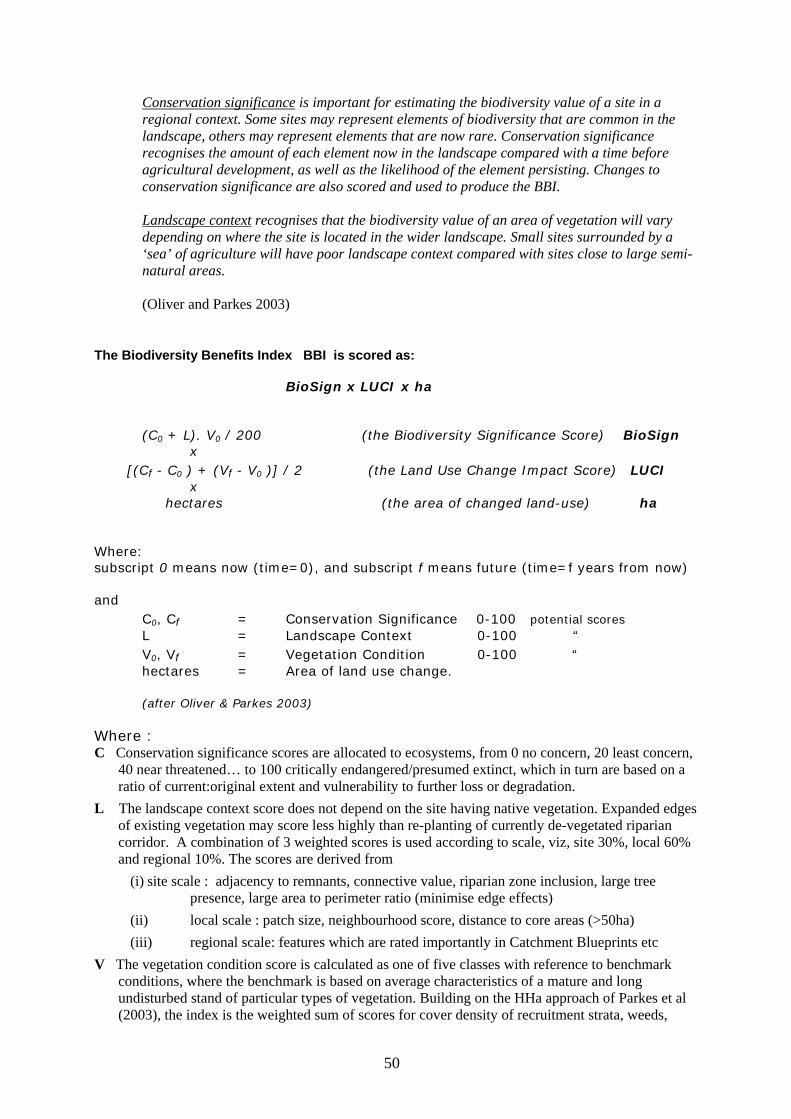
50

Conservation significance is important for estimating the biodiversity value of a site in a regional context. Some sites may represent elements of biodiversity that are common in the landscape, others may represent elements that are now rare. Conservation significance recognises the amount of each element now in the landscape compared with a time before agricultural development, as well as the likelihood of the element persisting. Changes to conservation significance are also scored and used to produce the BBI. Landscape context recognises that the biodiversity value of an area of vegetation will vary depending on where the site is located in the wider landscape. Small sites surrounded by a ‘sea’ of agriculture will have poor landscape context compared with sites close to large semi-natural areas. (Oliver and Parkes 2003)

The Biodiversity Benefits Index BBI is scored as:

BioSign x LUCI x ha

(C0 + L). V0 / 200 (the Biodiversity Significance Score) BioSign x

[(Cf - C0 ) + (Vf - V0 )] / 2 (the Land Use Change Impact Score) LUCI x

hectares (the area of changed land-use) ha Where: subscript 0 means now (time=0), and subscript f means future (time=f years from now) and

C0, Cf = Conservation Significance 0-100 potential scores L = Landscape Context 0-100 “ V0, Vf = Vegetation Condition 0-100 “ hectares = Area of land use change.

(after Oliver & Parkes 2003)

Where : C Conservation significance scores are allocated to ecosystems, from 0 no concern, 20 least concern,

40 near threatened… to 100 critically endangered/presumed extinct, which in turn are based on a ratio of current:original extent and vulnerability to further loss or degradation.

L The landscape context score does not depend on the site having native vegetation. Expanded edges of existing vegetation may score less highly than re-planting of currently de-vegetated riparian corridor. A combination of 3 weighted scores is used according to scale, viz, site 30%, local 60% and regional 10%. The scores are derived from

(i) site scale : adjacency to remnants, connective value, riparian zone inclusion, large tree presence, large area to perimeter ratio (minimise edge effects)

(ii) local scale : patch size, neighbourhood score, distance to core areas (>50ha) (iii) regional scale: features which are rated importantly in Catchment Blueprints etc

V The vegetation condition score is calculated as one of five classes with reference to benchmark conditions, where the benchmark is based on average characteristics of a mature and long undisturbed stand of particular types of vegetation. Building on the HHa approach of Parkes et al (2003), the index is the weighted sum of scores for cover density of recruitment strata, weeds,

51

organic litter, large trees, and coarse woody debris load, with additional elements of hollow-bearing trees, and cover and richness of benchmarked plant groups. (see Table 12.2.1 below) The long-term Potential Cover and Richness scores for use in the Vf term of the formula are those for benchmark vegetation conditions.

Table 12.2.1 Weightings used in BBI vegetation condition score V.

(source Oliver and Parkes 2003)

Vegetation condition attributes and values Attributes for BBI V score Value (%)

Richness of benchmarked plant groups 25 Cover of benchmarked plant groups 20 Cover or density of:

Recruitment 10 weeds 15 organic litter 05 large trees 15 hollow-bearing trees 05 wood load 05

TOTAL 100

Note that Cover (20 %) and Richness (25%), comprise the largest individual parts. Cover scores are debited for low health or dominance by exotics. Because the benchmarks for cover density and plant groups are presented as a range rather than absolute number as occurs in HHa, naturally occurring variation in the benchmark condition is accommodated. By examining the behaviour of the BBI function in a series of spreadsheet tables some conclusions have been made about the way the formulation works. These are as follows. The maximum potential score (for each hectare) from the first two factors BioSign and LUCI occurs when conservation significance improves from a current state of zero to a future state of 100 and vegetation is in benchmark condition at all times, i.e. (0+100).100/200 x [(100-0) + (100-100)]/2, or 10,000/200 x 100/2 = 2,500 However this score is highly unlikely in practice since it requires that the assessor already knows that although conservation significance C is low now it will become extremely important in future, eg because all other vegetation of that type will be cleared, or there is 100% certainty that something like a thylacine or Wollemi pine will inhabit the patch in future. It is more realistic to expect relatively minor changes in C, which means that changes in vegetation condition and landscape context are of greater practical significance in the BBI score. Where C is approximately constant and between 50 and 100, BBI scores peak at values from about 1000 to 1250 rather than the theoretical 2500 maximum. However it is clearly the case that high BBI scores can be obtained when there are substantial improvements in C over time (Cf >> C0). This is presumably designed to create a strong incentive for landholders to maintain or improve factors such as threatened species abundance and diversity and connectivity to their core habitat. Changes in vegetation condition affect the BBI score in a constant and consistent fashion. It was found that marginal gains in BBI are constantly diminishing with respect to increasing V0 irrespective of values of C and L. This means that where there is a choice between improving a low-scoring vegetation condition site and a high-scoring vegetation condition site, there will always be more BBI benefit obtained from an absolute change (e.g. +10 points for V score) on the lower V score site. The slope of the marginal BBI line however does depend on C and L. Where C and L are higher, the corresponding marginal gain in BBI is also higher. L essentially acts as a simple multiplier across all scenarios. Hence improvements are more highly valued on the higher-scoring C and L sites

52

BBI differs from HHa in that it incorporates both additive and interactive elements, but is similar to HHa in that both sum to a quality-adjusted total area equivalent. Cautious judgement may still be warranted with any area-weighted scorings, since 20 ha with score 10 may not always be equivalent to 2ha with score 100. The basic format of the BBI formula with two multiplied scores appears intuitively more sensible than an additive formula as used by HHa. Some outcomes are common to both methods, for example if (arbitrary) scores are BioSign = 32, LUCI= 76, BBI will be the same when the values are swapped, ie BioSign=76 and LUCI=32 . This implies that small changes in high biodiversity value sites have equivalent significance to large changes in low biodiversity value sites, for the same size area. This simple reversal of relative score value is the same for either multiplicative or additive scoring. However BBI is highest when LUCI and BioSign are equal, for any two numbers with the same sum. (e.g. as indicated above, 50x50 is greater than either 80x20 or 30x70). Thus in a multiplicative scoring method an absolute change in one index cannot be offset by the corresponding absolute change in the other; proportionate changes in one must be offset by proportionate changes in the other to achieve the same outcome and those relative proportions will depend on the initial scores and direction of change. In an additive scoring method however, adding of two scores implies that absolute value increases in variables are all of equal significance to the final score outcome. For example when using HHa, an increase of 5 points in the “lack of weeds” score (i.e. weed removal which changes the score/15 from 5-10 ) might be offset by a decrease of 5 points in the “landscape” score (e.g. fragmentation and connectivity worsen; moving the score/25 from 25-20) irrespective of current vegetation condition or landscape context . This seems less rational (notwithstanding being easier to calculate mentally) than where with a multiplicative index, the relative value of changes depend on context,, that is, on both landscape and conservation significance settings. Hence this BBI formulation exhibits desirable marginal properties and because the formula contains interactive effects for its component variables, it’s outcomes are also context dependent. However as a tool designed for incentives it has the result that most of the funds will be directed towards improvements at the lower ends of the scale. This may not be the most desirable outcome since it provides a relative disincentive for landowners to maintain or improve vegetation which is already in a high–scoring state. Changes in the BBI, for defined time periods, may be useful indicators of the “improve and maintain test” which is the primary regulatory condition of NVA 2003. However one limitation in using BBI for this purpose is that the assessment of recovery period ie the predicted rates of progress toward return to benchmark conditions of cover and richness after disturbance or revegetation, remains a matter for experienced field professionals (Oliver and Parkes 2003). A prediction of this nature introduces possibility of value-judgement bias, so modelled prediction may be preferable notwithstanding that no model is perfectly unbiased and that a form of model is yet to be considered and agreed. A calculated score like BBI maybe a useful indicator for sustainable forestry. However providing an absolute restriction on even short-medium term reduction in BBI will prevent PNF operations altogether, since short-term changes in cover must reduce the BBI score. A means of determining an acceptable frequency of time spent at less than benchmark condition (especially for cover) would need to be incorporated in the “improve or maintain” definition and the time-curve of BBI assessed accordingly. It is likely to be possible to conduct logging operations so that Vegetation Condition (V) is the main affected variable, mainly because of reduction in cover (n.b. crown-weighted basal area may be an equivalent and more easily measured proxy). For example selective or small gap (3-4x tree height) logging in PNF conducted with appropriate silvicultural goals, amongst a landscape matrix with higher quality habitat and vegetation condition, and where C and L are largely unaltered, 5 year post-logging BBI scores may be reduced by factors of 50%, with recovery (excluding roaded areas) to pre-logging

53

status before next logging cycle. This has not been examined in empirical or modelled form as yet, but an assessment will be included in forthcoming field trails by the SCU research team. A decline in site BBI over logging cycles will be a prima facie suggestion of non-sustainability in some attributes. However individual areas not meeting the non-declining trend criterion between logging cycles may also exist as a consequence of adaptive management experiments, and from short-term disruptive but low risk restorative action. Managers should not be penalised for adaptive management if they are able to counter the risks of losses appropriately. Documenting process and consequence and providing this to an PNF network for an adaptive management information pool may also be a rationale for seeking improvement methods which are optimal but have short-term negative outcomes (Wilhere 2002). Adopting adaptive management will means that if a management process is shown to not currently be providing a positive amount to the sustainability index, then changes are adopted that will improve the index as time progresses. The information to support this is drawn from the continual build up in the adaptive management network. However a purely regulatory use of BBI does not provide incentive to improve currently low BBI scores through silvicultural action or other means. It is not known whether BBI and the NSW Environmental Services Scheme are still currently funded and in use.

12.3 PVP developer and the BioMetric score The alternative to the market-based scheme of BBI is the regulatory approach of dEOAM (draft Environmental Outcomes and Assessment Methodology under NVA 2003). To assess whether “broadscale clearing” will improve or maintain biodiversity outcomes, dEOAM specifies calculation of a score called the BioMetric index; this score is thus a current draft regulatory instrument. The index is calculated using a spreadsheet tool as part of the “PVP developer” system. BioMetric v1.8 (DIPNR 2003) contains a modified version of the original BBI scoring system, as well as methods for assessing potential water quality, salinity and land (soil) degradation. It is not intended that BioMetric scoring methods will apply to PNF; however since the variables in BioMetric are very similar to those in BBI but the scoring method is different, a quick look at the implications of this will be made below. The BioMetric formula is currently proposed for both regulatory and incentive purposes, and is thus presumed to have some meaning as a surrogate for potential or actual environmental value. If that meaning is real it should be applicable in a very general way without needing to be tailored for different types of disturbance, so is worth comparing to other metrics for the PNF context. In the Biodiversity section of BioMetric, the first level of assessment is made for the actual “clearing” site according to purpose and context of clearing.

1. Thinning stems of common species <30cm DBH may occur provided it does not reduce densities to less than defined benchmarks in 0-10, 10-20 and 20-30cm DBH classes.

2. All clearing is excluded outright where more than 70% of the original estimated extent has been cleared in the CMA region AND current vegetation of that type in the proposed clearing zone has more than 50% of the benchmark minimum FPC AND perennial understorey or grasses constitute >50% of cover.

3. Any other clearing requires “improve or maintain” assessment

Assessments are made by establishing plots of 0.1ha, with one plot every 2 ha (max 10) for each listed (“Keith”) vegetation association (dEOAM 2003). As an example of the latter Table 12.3.1 shows the 11 listed vegetation associations which include Spotted Gum in the Northern Rivers CMA.

54

Table 12.3.1 A complete list of vegetation associations which include Spotted Gum in the Northern Rivers CMA. The number indicates % of original estimated extent now cleared. (source :dEOAM 2004 and BioMetric tool kit 2004) The site level assessment of the impacts of clearing on biodiversity score is made in accordance with the following (dEOAM 2004) The variables in the formula are explained in the Table on the next page. It is important to note this regulation is absolute in prescribing that clearing actions must result in an improved or maintained score. Some inconsistencies appear to be present in the draft. Since variables ‘b’ native overstorey projective cover, and ‘j’ fallen logs are both given 5% weighting, it appears that falling all overstorey except hollow-bearing trees and leaving the logs on ground will not affect the site value score, but felling and removal of 5 non-hollow bearing trees per hectare will ! It is important to note the strong implications of the final interactive components in this formulation. While the potential maximum for (a+b+c+d+e+f+g+h+i+j) = 300 when all attributes are in benchmark condition, (see overleaf) the contribution to total potential score form the remaining parts of the

55

formula are (a x f) =1800, (a x g) =900, (b x j) =225 and (h x i) =2700. Hence from a total of 5925 potential points, (nb the 6150 divisor in the formula appears to be an error) some 4500 or 76% of the site value is contingent on there simultaneously being overstorey species in the regeneration stratum and tree hollows, and native plant species richness plus ground cover, all at benchmark levels. Minor variation from a hypothetical benchmark ideal state in these heavily weighted components will very significantly diminish the BioMetric score. A preliminary field test of this scoring method was conducted in Sept 2005 as an SCU student exercise in adjacent recently lightly burnt and unburnt Clarence Lowland Spotted Gum sites in Myrtle State Forest south of Casino NSW. Both sites had evidence of recent (<10years) past logging. The site score results from 6 transects (3 each in burnt and unburnt) conducted according to the published methodology (DEC 2004) ranged from 54 to 65. Although the sample was too small for statistical inference, it was clear in analysis that the major cause of lost points was because variable f (“other” ground cover) did not meet the benchmark. The benchmark required that at there be at least 5 point intercepts at 5m intervals along a 50m tape transect, of vegetation other than grasses and shrubs, ie native forbs, ferns, vines etc. In discussion with experienced foresters, this benchmark seemed excessive for this type of forest. However had the benchmark been met, it would have been possible in theory to undertake some quite intensive ringbarking of valuable timber trees (canopy removal variable b) or removal of shrub understorey (variable e), without greatly reducing the BioMetric site score. It is hard to see why presence of forbs or ferns should have such relative importance relative to simplification of forest structures. This example illustrates the risk of over-weighting or inappropriately benchmarking a small number of variables in scoring methods. The BioMetric site value score is further adjusted for regional value according to % of original vegetation type cleared, and landscape level value which incorporates measures of surrounding current vegetation at 3 scales (10, 100 and 1000 ha), connectivity to adjoining blocks, and a further weighting based on size of disturbance (clearing) area. Passing the BioMetric “maintain or improve” tests will also require that there is no likely loss to any “predicted occurrence” of an individual of a threatened fauna species, area of habitat or key habitat features, unless such losses are offset by other actions in a PVP. (dEOAM secs 5.7 - 5.10). This appears to enlarge considerably on the TSCA 1995, which only requires that impacts are not “significant” as determined by the 8-part test in that Act. (sec 94 TSCA 1995), and does not require protection of “predicted occurrences”. This table is used in BioMetric to calculate a score relative to benchmark condition. It may be noted that compared to the BBI scoring weights in vegetation condition, number of trees with hollows has been changed from 5% to 30%, although the former also has a “large trees” variable with 20% weighting.

56

Table 12.3.2 The “PVP developer” BioMetric scoring system In summary the dEAOM is an indicator using landscape surrogates with a scoring structure superficially similar to HHa and BBI. It appears to offer some useful contributions to development of a landscape level scoring system for sustainability, but has a number of problems in its current form. These include:

• additive scores in Site Value which imply complete substitutability, • overweighted terms in the Site Value equation • reliance on mature state undisturbed vegetation as a benchmark • a zero value ascribed to nearby remnants <1 ha or distant remnants <100ha • Lack of distinction between fragments or contiguous blocks in Landscape Value • treating all surrounding vegetation as identical irrespective of floristic composition or

structural condition in calculating Landscape Value • discrete categories which encourage operating at the margins of the scoring system

57

13. Adaptive management Adaptive management refers to the systematic gathering and application of reliable knowledge, which is used to heuristically improve management actions over time (Wilhere 2002). It has been proposed as a means of developing improved management knowledge and understanding without needing to adhere to either prescriptive process or use surrogate site scores. There are two forms of adaptive management: passive and active. Passive adaptive management is conducted to produce predictive models, but the monitoring is conducted without the hallmarks of robust experimental design: controls, replication and randomisation. Thus, it cannot produce cause and effect relationships between the management actions and the targets of response. Under active adaptive management, however, management activities are conducted as a deliberate experiment, which can include a range of management treatments. Thus, active adaptive management is conducted with a statistically valid experimental design that is able to establish cause and effect relationships. However, active adaptive management is more complex and costly to implement (Wilhere 2002). The costs of quality research make adaptive management an expensive form of monitoring. However, case studies are not a substitute for statistically valid experimental design and they cannot guarantee that the knowledge gained is reliable (Wilhere 2002). An adaptive management framework applied to PNF in NSW would therefore involve monitoring of the individual elements that make up a scoring system such as BBI, and attempting to relate these to particular outcomes of different forms of logging in particular forest types, for example fauna population abundance or silvicultural response. However noting the wide confidence intervals where such correlations have already been attempted, the prospect of improving outcomes and management as a result of ad-hoc adaptive management experiments by a diverse group of owners in a diverse landscape does not seem bright. It is a natural human tendency to regard the plural of “anecdote” as “evidence”, and so adaptive management in PNF is most likely to continue to be a word-of-mouth or personal-experience based process. As such it will unfortunately be of little value because stochastic processes in unreplicated trials will lead to different outcomes. This is not to down-play the value of local knowledge and experience but only to suggest that it cannot be generalised in the way that most would like to believe. Therefore adaptive management in its usually intended passive sense is unlikely to provide a path towards sustainability. At some point the efficacy of patch- and landscape-level biodiversity sustainability strategies must be assessed by inferential research rather than ad-hoc heuristic discovery. Despite the problems outlined above, the use of “focal” or “indicator” species may be the only practical approach to establish such a link. This is because of the costs of a complete species inventory, sampling with sufficient intensity to overcome uncertainties regarding many species’ responses to disturbance, and difficulties in simply identifying species reliably, may be prohibitive (Burgman & Lindenmayer 1998; Carignan & Villard 2002). If such approaches are to be used, however, there must be a clear link between the reasons for monitoring and the indicators of response. Moreover, the limitations of such an approach (focal species should not be assumed to be general ecological indicators) must be recognised and incorporated into the decision-making process. The best value from a focal species approach is obtained by including as many species as is practically possible (Carignan & Villard 2002; Rolstad et al. 2002). For example, if the issue to be monitored is forest fragmentation, then a number of species, each responding to fragmentation at different spatial and temporal scales, should be used. Similarly, monitoring the effects of the loss of hollow-bearing trees should involve species requiring both small and large hollows.

58

14. Towards an improved index of sustainability 14.1 Rationale for, and form of a sustainability index Forests, even if greatly simplified in the form of monoculture plantations, provide far greater biodiversity conservation values than cleared pasture or cropland (Borsboom et al 2002, Lindenmayer 2002c). Since around half of the forested area of northeast NSW is privately owned, PNF is an integral part of the matrix of reserved and managed forest. Therefore maintaining a substantial forest cover on private land will make a significant contribution to the conservation of regional biodiversity, even if that forest is intermittently disturbed by logging operations. The biodiversity values of the NE NSW region may decline if either

(i) the forest is permanently cleared, which is of critical importance because of the presence of endemic or rare species or because it serves a connective function;

(ii) forest structure is severely simplified or degraded over large areas for long periods of time; or

(iii) critical habitat features of the forest are lost (e.g. absence of hollows, or absence of seasonal food sources notwithstanding abundance of hollows) and these cause or substantially increase the likelihood of landscape-level extinctions of populations of target or rare species

Therefore a sustainability indicator must be able to detect these events. Turner et al (2003) reviewed the outputs of research carried out to evaluate the Montreal C&I, and concluded that “a universal indicator of biodiversity [sustainability] is unlikely to be identified”. While it is not possible, therefore, to guarantee or “prove” ESFM is occurring in PNF, there are two main approaches which can be used as interim, precautionary indicators.

• standards & criteria. (relevant for strategic planning; requires auditable compliance with processes; suitable as a bottom line test for “maintain” environmental outcomes)

• scoring : for example Habitat Hectares; Biodiversity Benefits Index BBI, BioMetric (PVP developer) (relevant for operational planning; uses evidence-based measures of outcomes; suitable as a measure for “improvement” of environmental outcomes; site level information can be aggregated to provide regional “standards” )

A checklist with fundamental harm-prevention safeguards for soil and water and threatened species may be a common element in both approaches. Since the NVA 2003 allows actions to “maintain or improve”, and planning is appropriately done at both strategic level (agency) and operational level (landowner), both approaches will have a role as sustainability indicators. Certification to a standard will require that management processes include monitoring and aim for continuous improvement, however standards schemes such as MC&I and AFS offer no statement about outcomes. A self-assessment program using a structural indicator, supported by externally funded fauna surveys and sampling, could be used in a comparative fashion across the landscape and over time. The scoring methods are evidence-based and it should be easier and more valuable to record, analyse and report field data than to undertake certification procedures. Scoring systems also offer greater decision-making guidance with regard to prioritising actions across the landscape and different scales.

59

To assess improvement in site condition and sustainability, we prefer the structure of the BBI indicator rather than either HHa or BioMetric in dEOAM. No judgement is yet being made about the variables to include or their relative weighting. PNF is not possible with the BBI or BioMetric indices in their current form; the index must be time-integrated (i.e. tolerable variance for given durations defined) if it is to be used for PNF purposes. Field testing of BBI and other indicators may lead to some re-weighting of existing variables. BBI’s market-incentives based approach can stimulate improvements in vegetation condition, rather than using a regulatory approach which offers no benefit for moving beyond a current poor condition. The main perceived sustainability issues for PNF in NE NSW are

• the deterrent to providing habitat which arises from the private costs of providing public goods & services (including risk assessment such as fauna survey)

• deteriorating silvicultural condition, in which future sovereign risk now plays a major part • additional costs and inefficiencies likely to arise from conforming to prescribed processes

rather than attaining outcomes. The effect of native forestry operations on soil condition (nutrients, structure and bulk density) and water quantity (flow regime) and quality (turbidity, sedimentation, eutrophication) do not appear to be a major cause for concern at present at a regional scale in Australia, provided that roads and stream crossings are adequately sited, designed and maintained, and extent of catchment disturbance is less than 20% at any given time (see section 10 this report). Obtaining baseline information for soil and water impacts of PNF in UNE NSW to make a scientific evaluation seems highly problematic, and perhaps unnecessary if simple standards are adhered to. It should be noted that clearing (including PNF) on steep land >18o slope or in riparian zones on named watercourses has long been subject to consent and conditions in NSW. To address the sustainability issues we feel it is necessary to

• Minimise cost of habitat assessment and privately provided duty-of-care services • Provide tools which illustrate benefits of good silviculture and self-inflicted penalties of bad

silviculture (i.e. landholders undertaking high-grading which causes deterioration in productivity).

• Define desirable outcomes and suggest a range of means for achievement, rather than prescribe a single pathway

Ideally, a sustainability index for PNF sites in NSW would provide for these needs as well as provide an objective means to prioritise the targets for incentives to “maintain or improve” environmental outcomes. We do not see that an index would be useful or equitable as a lowest-common denominator regulatory backstop. A simple checklist with fundamental harm-prevention standards for soil and water and threatened species may be sufficient for regulatory safeguards. Instead, we suggest that if the index has a marketable value, landholders can make their decisions based on economic consequences. Aggregating reports or audit samples of index scores may be useful also as a strategic monitoring and regional planning device. In this form it becomes a tool for market adjustments by state resource management agencies, much as aggregated economic indicators are used by the Reserve bank in setting interest rates. The 3 forms of index briefly examined in this report (section 12) are either missing some important features or have inappropriate structures for use in determining and monitoring sustainability of PNF. We will attempt to improve on these indices by developing a new form, but using the same general approach of scoring based on vegetation structural attributes, conservation significance, and landscape context that are included and weighted according to a checklist of fundamental ecological principles.

60

In the discussion below BBi refers to an as-yet undefined Biodiversity Benefits indicator score, with similar formula but some additional or modified variable to those in ‘BBI’ (sec 12.2) . In the second phase of the research we will be defining and field-testing BBi. BBi considers only habitat values. Some guidance for timber productivity also seems worthwhile, so we will also be developing a Silvicultural Sustainability Score ‘S3’, based on stand condition and development over 30 years as illustrated in Fig 8.3 Two steps are envisaged for stand level assessment of BBiS3.

1. A plotless inventory which will provide useful data for timber valuation, silvicultural condition assessment (inputs to S3), inputs to a growth model for stand projection, and calculation of the structural components of BBi. Jay (2005a) describes a method which provides this within about 15 minutes per plot measure.

2. A checklist of habitat features and attributes, using class intervals of equal importance.

In the PNF context, the BBiS3 index would be used to compare pre- and post-harvest scores for a range of factors and conditions to determine whether environmental outcomes are “maintained or improved”. However the index must allow short-term reductions in site scores where these can be reasonably predicted to recover in a reasonable time, or are offset by increases in the index on other sites collated within a property PVP (offsets). Even a “benign neglect” site will indicate some change in condition and score if it is not currently in the benchmark state. Projections of the recovery of the site score can be made using stochastic modelling with a suitable mixed-age mixed species forest growth model. At least two post-harvest reference points could be included, ie immediate and at the time of next cutting cycle (e.g. 10-20 years depending on operation type and site conditions). Monitoring and comparison of the predicted and the actual index at interim times could be a useful adaptive management tool. Our proposed BBi score will start with a coarse filter approach. This will have a strong focus on forest structure and future stand development at the site scale, and a broader patch and landscape-context metric which incorporates fragmentation, connectivity and structural condition scores for surrounding forest. We expect to use many of the same variables already in dEOAM and HHa and BBI though perhaps in different ways. We expect to add or modify some variables such as forest structures, hollow counts, proximity to riparian zones. Our use of the variables is likely to involve both additions and multipliers, the relationship between some variables will not be linear, and the measures of some may be continuous rather than discrete to avoid incentives for operating at the margins. We note the use of no more than 10 variables in the HHa approach of which only 3 are at landscape level. The combination of measures used will be agreed by a steering committee overseeing the suite of PNF projects with expert advice, and allow comparison with the Victorian project. For scoring of fauna habitat, a “passport application” approach is envisaged. The method has not yet been finalised and is outlined rather than defined in the following discussion. A “passport approach” means that point-scores are allocated in a number of different checklist columns for habitat features expected to be suitable for focal species groups eg arboreal marsupials, reptiles, ground mammals, bats, insectivorous birds, other birds. We do not anticipate including predators in the columns because of the difficulty in relating the impact of land management on individual holdings to species with large home ranges. Where an owl roost or quoll den may be in the actual stand proposed for logging, these will be protected through either general structural conditions or fine-filter assessment methods.

61

In the same way that 100 points are needed to apply for a passport or a bank account or a driver’s licence, wildlife-BBi points can be obtained by using some items in column A, some from B, etc, so this metric will be a simple addition. This implicitly recognises that it is not necessary for each and every hectare of forest to supply all habitat values at all times. However it is important that there be some temporal continuity in the scoring system, and that a critical minimum number of total points be scored from each of several of the columns so that some usable habitat is represented. A few high-scoring columns is better than many low scoring columns, since the latter may offer no actually usable habitat. Like the alternatives of prescriptive habitat retention or direct fauna monitoring, this “passport” approach is for site level use only; at landscape or regional scale impractically intense monitoring of site values and prescriptive spatial management would be necessary. Table 14.1 provides an example albeit incomplete, since weightings, attributes and fauna groups are yet to be finalised. These numbers used are purely illustrative at this stage. If there were say 10 fauna groups, the default total for the table is 100 points but it may be higher or lower. The total table potential passport points will vary according to the “conservation significance” factor CS in BBi. For example , if the area was particularly important for reptiles, that column may be re-scaled to a total of 30, making a table potential total of 120. The landowner would then find it easier to gain “points” by managing for attributes that suit reptiles than for other fauna. The total number of available points reflects the general importance of the site for habitat. The passport approach would operate by tallying the points from columns which have a minimum score (after multiplier) of say 60% of the column potential. The total tallied points would then be used as an input in BBi. We have yet to determine whether this should be used additively, non-linearly, or logarithmically. Table 14.1 Passport scoring approach for wildlife-BBi

Fauna group A B C D Habitat Diurnal micro reptiles ground Attribute birds bats mammals rocky outcrop 3.0 fallen logs 1.0 2.0 winter flowering nectar sp. 1.0 Mature trees 1.5 Large branch hollows Etc etc…. .... ... ... ... TOTAL 7.5 3.5 5.5 2.5 Prev period multiplier 1.5 0.75 1.0 1.5 The multiplier is designed to reward continuity from previous period, and value new habitat features or changes conservatively. The example indicates multipliers of 1.5 (previous column score at last harvest event >6), 1.0 (no previous column score, or score 4-6) and 0.75 (previous score < 4). In principle the values are exchangeable between times and columns for a given stand. Provided the multiplier column scores of habitat attributes x area for the entire forest ownership is not deteriorating from one cutting cycle to the next, then the operations can be a priori considered to be sustainable The passport score, like BBi as described below, will be a continuous annual calculation of scores from pre-logging year and post-logging year, and all stand development stages through to next cutting cycle. This may not be as complicated as it sounds, since many of the attributes will not change much in a 10-20 year period, and those that do change can be reasonably predicted from the forest stand growth projection and a post-harvest measure.

62

Since the passport score will be used in the BBi indicator and we envisage this having some economic value in market-based conservation programs, there will be incentive for the landowner to measure, record and report the scores and their component attributes, and of course maintain a high score. Accuracy of claims must be subject to some percentage of audit, in the same way that tax returns are in general self-assessed but subject to audit. Such a system also integrates well with the adaptive management concept since it provides both a record and a forecast which can then be evaluated over time. It will also scale well from site to landscape. There is scope for a regulatory agency to flag site importance by allocating column weights on particular sites; higher weights will make it easier to claim economic benefits from the index which therefore forces both the agency and landowners to weight their priorities sensibly. The “passport” approach was suggested by a forest owner on the research team (Robert Dyason), and appears to be flexible enough to cater for temporal changes and differing site potentials. We will be investigating field application in phase II of the research should it be funded.

14.2 Integrating time effects in the sustainability index The three forms of index discussed previously in this review were calculated by predicting outcomes of a particular management action. A tallied score determined whether there is a movement towards or away from a benchmark ideal. All indices discussed used a similar ecological community in mature undisturbed condition as a benchmark. We propose using a similar benchmark in BBiS3 but in a different way. Suppose that it is possible for a forest site to return to benchmark condition from a “worst-case reversible” biodiversity state. If it cannot return, then the current condition is not worst-case, it is irreversibly different. The most heavily disruptive but still sustainable action is then definable as that which intermittently causes a disruption from benchmark such that the ideal state becomes the worst-case; a stand-replacing wildfire such as those that devastated some southern Australian National Parks in recent years serves as a “natural” example. A definable ideal end-state for any given site is open to argument , but suppose for a moment that one exists, and it can be captured by a single score, eg BBi. (or alternatively, suppose that many qualitatively equally desirable but structurally different end-states exist, in which case they should have identical BBi scores and the analysis is unchanged). On various sites, we can envisage a trajectory from an initial worst-case reversible state to the end benchmark state, taking a certain period of time for the journey. BBi I score

W

‘ to period of interest t t1 time (years) Figure 14.2.1 Site scoring for BBi over time:

W = worst case reversible I =ideal benchmark score N= current score now

N

63

In Figure 14.2.1, the horizontal axis is a time line and the BBi score at any given time for a certain site can be shown on a vertical axis. The ideal and worst case reversible situations can be measured on this axis, and are shown in the figure as dotted lines corresponding to their BBi score. On this hypothetical site, the periodic BBi score is shown by the solid line prior to now, where now= to We can assume that at some long prior point in time that the solid line started from I, the ideal benchmark score. Let us say that t= t1—t0 is the time it will take the site to return to the benchmark condition under a policy of benign neglect, from it’s worst case site score (dashed trajectory - note worst-case is not BBi=0, since we assume there are some site conditions with lower BBi score which are effectively irreversible). Now consider (Figure 14.2.2) that instead of only a single site, the same concept applies to a property which is constituted of a number of separate sites. The solid line is then a sum of site scores. Similarly there is a definable IT and WT for the property as a whole, but noting that if landscape scale heterogeneity is desirable, then IT for the site as a whole will be less than the sum of all individual site I (or we make I context dependent, which is unnecessarily complicated). We will develop this important concept further in the second phase of this research project. BBi score I B

H C W D

‘ to period of interest t t1 time (years) Figure 14.2.2 Site scoring for two sites When H is halfway between I and W, BC= CD = (I-W)/2 and the area IWB = IHCB since both are half IWDB. The thin solid line is one example of a potential future trajectory of BBi scores. If we now assume that the public has an economic interest in the BBi score, and further that the landholders duty of care extends to providing half of the BBi score between ideal and worst case before expecting payment for provision of the public goods, then the land-use is ethically and economically neutral if sum of BBi scores in any given period of ‘t’ years is not < t(I-W)/2 which is the area IWB = IHCB. Suppose t is 50 years. If the cumulative sum of 50 year BBi scores exceeds the critical amount of IWB (=IWDB), then the landholder has a biodiversity credit. If the sum total falls below then the landowner has a debit or loss of credit (Figure 14.2.3) which may or may not be compensated for by cash income from the management actions which have occurred (such as partial clearing or other actions which have resulted in a decline in the property’s PVP score). To be clear, we are not advocating regulatory penalties for falling below the line HC, although falling below the WD line is by the definitions here, a change of land use from permanent forest condition and would require a clearing permit under NVA 2003.

64

Figure 14.2.3 Site scoring showing biodiversity credit and debit If the landowner receives some economic benefit from providing BBi beyond duty-of-care, then maximum benefit will be received when the cumulative area spent above the line CH multiplied by its BBi credit value, is equal to the income gained from time spent below the line. In other words the weighted values of the striped CREDIT area is equal to the weighted value of the stippled DEBIT area. At the landscape scale, a regulator or “market maker” can provide incentive to maintain or improve environmental condition in high priority areas by raising the value of BBi incentive payments in those areas. (e.g. regional scale corridors, under-reserved or over-cleared ecosystems). If the lansdcape is becoming too homogenous at either the high or low end of aggregated scales, then the price of BBi credits can be raised or lowered accordingly to induce changes in site management. vanBueren (2001) describes a similar “baseline and credit” system used as a market instrument for controlling pollution outputs. A firm with a surplus of credits can either sell them or ‘bank’ them for later use. A further criterion to make this process acceptable is that the credit-debit balance should be maintained over some reasonable interval; we suggest 30 years as a starting point which is within the scope of current modelling. (t=30) If ‘t’ is a much longer time, eg 100 years, it seems unreasonable to suggest that the property-level score could be in debit for the first 80 years and credit for the next 20. It may be reasonable to do this for a single site, but less so for a landscape. Using this assessment it might be expected in many cases that “benign neglect” would result in lower cumulative score balances than positive silvicultural and management intervention. (Ref Fig 8.3). We are not advocating penalties against benign neglect nor in favour of compulsory intervention. We are rather suggesting that if silvicultural action can result in equivalent or better outcomes than benign neglect on a measurable objective index, then notwithstanding short-term moves away from the benchmark that silvicultural action should be a preferred and encouraged process rather than being replaced by a hands-off approach. The “maintain or improve” condition if interpreted in absolute form, would eventually result in all sites returning to benchmark condition and then no change allowed in any of them, which basically precludes management from there on. However it is important to recall that the legislation requires the test to be carried out “in accordance with the principles of ecologically sustainable development”. These principles, as previously discussed mean that socio-economic factors are to be included. Therefore it is important that an index of sustainability can accommodate movement “away from” a benchmark ideal in the short term, when this is reversible and results in some socio-economic benefit. In this way the index is not always directed towards some single homogenous ideal which may not even be possible for that site in any reasonably foreseeable time. A model-based approach could establish an index score which is the sum of annual deviations from a reference time-line. We will be developing these ideas further in the second phase of this research.

65

14.3 Conclusion The PNF landowner’s role in sustainability assessment will be to use relatively straightforward self-assessed scores and checklists at the site-level. We expect these planning tools can provide a means for landowners to demonstrate that their PNF actions are likely to be sustainable, and therefore that

(i) they are operating in accordance with the current “sustainable forestry” exemption AND that they pass the “improve or maintain” test of the new legislation, and

(ii) the onus of proof then reverts to a compliance monitoring agency to state why a given site is

NOT meeting the “maintain or improve” condition. We propose that a regulatory agency’s role, in accordance with the administrative mechanisms proposed for PNF in the Regional Forest Agreement of March 2000, would be to

(i) aggregate BBiS3 site assessments for use in Montreal-based indicators and thus monitor the implementation of ESFM at a landscape and regional scale,

(ii) audit compliance with soil and water and threatened species safeguards

(iii) prioritise and co-ordinate financial benefits in the proposed credit/debit system

(iv) provide supportive advice for use of BBiS3 as a management planning tool

(v) sponsor any research required to improve the reliability and confidence levels of the index.

66

15. References 1. ABARE 2001 Alternative policy approaches to natural resource management ABARE

Canberra

2. AFG (Australian Forest Growers) 2005, Certification To The Australian Forestry Standard For Small-Scale Growers Accessed on-line at www.afg.asn.au/projects/afs_small_scale_growers.html 10 May 2005

3. AFS (Australian Forestry Standard) 2003 Background papers Accessed online 10 May 2005 at www.forestrystandard.org.au/index.html

4. Andelman, S.J., Fagan, W.F., 2000. Umbrellas and flagships: efficient conservation surrogates or expensive mistakes? Proceedings of the National Academy of Sciences of the United States of America 97, 5954–5959

5. Anon 1995 National Forest Policy Statement - A New Focus for Australia's Forests Accessed on-line 10 May 2005 at www.affa.gov.au/content/publications.cfm?ObjectID=CDA4CAF9-D118-4E13-AAC472AC7603EBE5

6. Armsworth, P. R., and J. E. Roughgarden. 2005. The impact of directed versus random movement on population dynamics and biodiversity patterns. The American Naturalist 165:449-465.

7. Arpat, O., L. L. Getz, and M. K. Oli. 2004. Demography of fluctuating populations: temporal and phase-related changes in vital rates of Microtus ochrogaster. Journal of Animal Ecology 73:201-215.

8. Atlegrim, O., and K. Sjöberg. 2004. Selective felling as a potential tool for maintaining biodiversity in managed forests. Biodiversity and Conservation 13:1123-1133.

9. Attiwill, P. M. 1994a. The disturbance of forest ecosystems: the ecological basis for conservation management. Forest Ecology and Management 63:247-300.

10. Attiwill, P. M. 1994b. Ecological disturbance and the conservative management of eucalypt forests in Australia. Forest Ecology and Management 63:301-346.

11. Bauhus, J. 1999. Silvicultural practices in Australian native State Forests – an introduction. Australian Forestry. 62(3):217-222.

12. Baur, G.N. 2001. Silviculture Notes for New South Wales. Institute of Foresters of Australia. State Forest of New South Wales. Coffs Harbour. CD Rom.

13. Bassett, O.D. and G. White 2001 Review of the impact of retained overwood trees on stand productivity Australian Forestry 64(1):

14. Belbin L. 1991 The Analysis of Pattern in Bio-Survey data Chapt 23 in Margules C.R. and M.P Austin (eds) Nature Conservation: Cost Effective Biological Surveys and Data Analysis

15. Bennet L.T. and M.A Adams 2004 Assessment of ecological effects due to forest harvesting: approaches and statistical issues. Journal of Applied Ecology 41 (4), 585-598.

16. Bentley, J.M. & Catterall, C.P. 1997, ‘The use of bushland, corridors and linear remnants by birds in south east Queensland, Australia’, Conservation Biology, vol. 11,pp. 1173–89.

67

17. Bolen, E. G., and W. L. Robinson 2003. Wildlife Ecology and Management, Fifth Edition. Prentice Hall, Inc., Upper Saddle River, New Jersey.

18. Borg, H., A. Hordacre and F. Batini. 1988 Effects of logging in stream and river buffers on water courses and water quality in the southern forest of Western Australia. Australian Forestry 51 2

19. Borsboom, A.C., J. Wang, N. Lees, M. Mathieson and L. Hogan 2002 Measurement and integration of fauna biodiversity values in Queensland agroforestry systems RIRDC JVAP report no. 02/044 QDN-6A Accessed on-line 10 May 2005 at www.rirdc.gov.au/reports/AFT/02-044sum.html

20. Bren, L. J. 1980 Hydrology of a small, forested catchment Australian Forest Research, 1980, Vol.&nbsp10, No.&nbsp1, pp.&nbsp39-51, 15 ref.

21. Bren, L. J. 1995 Aspects of the geometry of riparian buffer strips and its significance to forestry operations Forest Ecology and Management, 1995, Vol.&nbsp75, No.&nbsp1/3, pp.&nbsp1-10, 14 ref.

22. Bren, L. J. 1997 Effects on increasing riparian buffer widths on timber resource availability Australian Forestry 60 4 260 263

23. Bren, L. J. 2000 A case study in the use of threshold measures of hyrodologic loading in the design of stream buffer strips Forest Ecology and Management 132 243 257

24. Brook, B. W., M. A. Burgman, H. R. Akcakaya, J. J. O'Grady, and R. Frankham. 2002. Critiques of PVA Ask the Wrong Questions: Throwing the Heuristic Baby Out with the Numerical Bath Water. Conservation Biology 16:262-263.

25. Brown D.M., H.B Hines, S.Ferrier and K.McKay 2000 Establishment of a biological database for regional conservation planning in northeast New South Wales Phase I (1991-1995) NPWS Hurstville NSW

26. Burgman, M. A., and D. B. Lindenmayer 1998. Conservation Biology for the Australian Environment. Surrey Beatty & Sons, Chipping Norton, NSW.

27. Burgman, M., Ades, P., Hickey, J., Williams, M., Davies, C. and Maillardet, R. (1998). Methodological guidelines for the utility and statistical validity of survey and monitoring programs. Final Report to FWPRDC on PN 98.803. 33 pp.

28. Calaby, J. H. 1966. Mammals of the upper Richmond and and Clarence Rivers, New South Wales. Page 55, Melbourne.

29. CARE, GE, EBC (Centre for Agricultural and Resource Economics, Gillespie Economics, Environment & Behaviour Consultants) 1999 Regional Impact Assessment : Upper North East CRA Region NSW and Cwth govts CRA project numbers NU 12/ES & NA 39/ES

30. Cary J., T. Webb and N. Barr 2002 Understanding landholders' capacity to change to sustainable practices. Bureau of Rural Sciences, Canberra Publictn 12921

31. Carignan, V., and M.-A. Villard. 2002. Selecting indicator species to monitor ecological integrity: a review. Environmental Monitoring and Assessment 78:45-61.

32. Carlyle, C., Snowdon, P., Polglase, P., Nambiar, S., Smith, T., Simpson, J. and Bubb, K. (2002). Soilbased Information for Developing Sustainable Plantation Forestry in Australia. Final Report to FWPRDC on PN 99.801. 94 pp.

33. Caro, T. M., and G. O'Doherty. 1999. On the use of surrogate species in conservation biology. Conservation Biology 13:805-814.

68

34. Catterall, C.P. 1993 The importance of riparian zones to terrestrial wildlife. In; Ecology and management of riparian zones (Eds S.E. Bunn, B.J. Pusey and P. Price) Occasional Paper no 05/93, LWRRDC, Canberra pp 41-52

35. Chesson J. 2002 Sustainability Indicators - Measuring our Progress Accessed on-line 10 May 2005 at www.affa.gov.au/content/output.cfm?ObjectID=8B041206-8D37-4C82-87D2A2FD6F65C628

36. Chikumbo, O., R.D. Spencer, B.J. Turner and S.M. Davey 2001 Planning and monitoring of forest sustainability: an Australian perspective Australian Forestry 64(1) 1 7

37. CIE (Centre for International Economics) and CSIRO 2000 Determining the Effectiveness of Vegetation Management Programs – Measures and Methodologies RIRDC JVAP Publication no 99/130 Project no. MS967-43

38. Clark, T. W., R. M. Warneke, and G. G. George. 1991. Management and conservation of small populations. Pages 1-18 in T. W. Clark, and J. H. Seebeck, editors. Management and Conservation of Small Populations. Proceedings of a Conference held in Melbourne, Australia September 26-27, 1989. Chicago Zoological Society, Chicago.

39. Clarke, F. 2005 A small grower’s viewpoint of the Australian Forestry Standard. Aust Forest Grower magazine; Summer 2005 27(4) p.15

40. Combe, M. 1998 Resource profile of "high-graded" dry hardwood forests: implications for improving productivity in Dyason et al (eds) Aust For Growers Biennial Conference Proceedings, Lismore NSW 6-9 July 1998

41. Cooper C.B., and J. R. Walters 2002 Independent effects of woodland loss and fragmentation on Brown Treecreeper distribution Biological Conservation 105:1-10

42. Cornish, P. M. 1989 Water quality in logged eucalypt forest near Bega, NSW, during a nine year period. Australian Forestry 52(4)

43. Cox M.P., C.R Dickman and J.Hunter 2003 Effects of rainforest fragmenetation on non-flying mammals of the Eastern Dorrigo Plateau, Australia Biological Conservation 115:175-189

44. CSIRO 2005 Forests for Tomorrow Accessed on-line 10 May 2005 at www.fwprdc.org.au/content/ pdfs/Forests%20for%20tomorrow.pdf

45. DAFF 1998 Framework of Regional Level Criteria & Indicators of Sustainable Forest Management , Accessed on-line 10 May 2005 at www.affa.gov.au/content/publications.cfm?ObjectID=D4696EF3-97E9-4D27-A00D0D586164433A

46. DAFF (Commonwealth Dept of Agriculture Fisheries and Forestry) 1999 A report on forest wood resources for the upper and lower north east NSW CRA regions Accessed on-line 10 May 2005 at www.affa.gov.au/content/output.cfm?ObjectID=066592B0-8A2B-4DB3-A639B791170BB62C

47. DAFF 2005 Certification of Forest Management in Australia Accessed on-line at www.affa.gov.au/content/output.cfm?ObjectID=D2C48F86-BA1A-11A1-A2200060B0A03634 10 May 2005

48. Davey, S. M. 1989 Thoughts towards a forest wildlife management strategy. Australian Forestry 52(2):56-67

49. Di Stefano, J. (2001). Power analysis and sustainable forest management. Forest Ecol. Manag., 154, 141–153.

69

50. DIPNR (NSW Dept of Infrastructure Planning and Natural Resources) 2003 Environmental Services Scheme ESS Accessed on-line 10 May 2005 at www.forest.nsw.gov.au/env_services/ess/default.asp

51. DIPNR (NSW Dept of Infrastructure Planning and Natural Resources) 2004 PNF Code : Proposed Native Forestry Regulation unpublished draft version 4, May 2004 DIPNR Private Native Forestry Working Group

52. Dore, D., I. Elsley and W. Bratby 1999 Development of systematic, quantitative silvicultural prescriptions for the modelling of forest operations in NSW Australian Forestry 62(2)

53. Eyre T.J and Norman P. 2004 The development and implementation of landscape metrics for reporting forest fragmentation at field and landscape levels (316KB) FWPRDC Project No PN99.807

54. Eyre, T. J., and A. P. Smith. 1997. Floristic and structural habitat preferences of the yellow-bellied glider (Petaurus australis) and selective logging impacts in southeast Queensland, Australia. Forest Ecology and Management 98:281-295.

55. Fahrig, L. 2003 Effects Of Habitat Fragmentation On Biodiversity Annual Review of Ecology, Evolution, and Systematics Vol. 34: 487-515

56. Fahrig, L. 2001. How Much Habitat Is Enough? Biological Conservation 100: 65-74.

57. Failing, L. and R.Gregory 2003 Ten common mistakes in designing biodiversity indicators for forest policy. J. Environ Manage. 2003 Jun;68(2):121-32.

58. Faith, D.P., Walker, P.A., Ive, J.R., Belbin, L., 1996. Integrating conservation and forestry production: exploring trade-offs between biodiversity and production in regional land-use assessment. Forest Ecology and Management 85, 251–260.

59. Fanning D. 1995 Fauna Survey Report of rthe Tenterfield Management Area Gunninan Consultants Sydney

60. Faucheux, S., D. Pearce and J.Proops (eds) 1996 Models of sustainable development Edward Elgar, Vermont USA

61. Ferguson, I. S. 1996 Sustainable forest management Oxford University Press; Melbourne, Oxford

62. Field, S.A., A. J. Tyre, N. Jonzen, J.R.Rhodes and H.P. Possingham 2004 Minimizing the cost of environmental management decisions by optimizing statistical thresholds Ecology Letters, (2004) 7: 669–675

63. Figgis P., 2004 ‘Conservation on Private Lands: the Australian Experience’ IUCN, Gland,Switzerland and Cambridge, UK. i to 31 pp. Accessed on-line 28 May 2005 at http://www.acfonline.org.au/docs/general/00532.pdf

64. Fleishman, E., C. J. Betrus, R. B. Blair, R. MacNally, and D. D. Murphy. 2002. Nestedness analysis and conservation planning: the importance of place, environment, and life history across taxonomic groups. Oecologia 133:78-89.

65. Fleishman, E., R. B. Blair, and D. D. Murphy. 2001. Empirical validation of a method for umbrella species selection. Ecological Applications 11:1489-1501.

66. Florence, R.G. 1996. Ecology and Silviculture of Eucalypt Forests. CSIRO, Canberra. 413 Pp

67. FNSW (Forests New South Wales) 2005 Sustaining our Forests. Bush Telegraph magazine Autumn 2005:14-15 (see also www.forest.nsw.gov.au/esfm/)

70

68. FNSW (Forests New South Wales) 2002 Social, environmental and economic report 2001/0. State Forests of New South Wales, Sydney. 68 pp.

69. FNSW (Forests New South Wales) 2004 Wildlife survey sightings. Accessed on-line 10 May 2005 at.www.forest.nsw.gov.au/publication/e_sv/pdfs/values_04biodiversity.pdf

70. Foppen, R. P. B., J. P. Chardon, and W. Liefveld. 2000. Understanding the Role of Sink Patches in Source-Sink Metapopulations: Reed Warbler in an Agricultural Landscape. Conservation Biology 14:1881-1892.

71. Fortech 1998 Forest Industry Development Options: Northeast region (NSW CRA) NSW and Cwth govts

72. Frederick S., G Lowenstein and T O'Donoghue 2002 Time Discounting and Time Preference : A Critical Review Journal of Economic Literature, vol. 40, no. 2, pp. 351-401 Accessed online 10 May 2005 at www.hss.caltech.edu/~steve/files/FredLoewOD.pdf

73. Gibbons P. and D. B. Lindenmayer 1997 Developing tree retention strategies for hollow-dependent arboreal marsupials in the wood production eucalypt forests of eastern Australia Australian Forestry 60(1)

74. Gillespie, R. 2000 Economic Values of native vegetation in NSW. NVAC Background paper no. 4. ; NSW Dept Land & Water Conserv.

75. Goldingay, R. L., and D. A. Newell. 2000. Experimental rock outcrops reveal continuing habitat disturbance for an endangered Australian snake. Conservation Biology 14:1908-1912.

76. Goldingay, R. L., and D. J. Sharpe. 2004. How do we conserve the Squirrel Glider in Brisbane's urban matrix? Pages 663-677 in D. Lunney, editor. Conservation of Australia's Forest Fauna, 2nd Edition. Royal Zoological Society of New South Wales, Mosman, NSW.

77. Gullison R.E 2003 Does certification conserve biodiversity ? Oryx, 37(2), 153–165

78. Hancock C.N. 2003 Factors affecting the physiognomy and species richness of plant communities of valleys of the Darling Plateau, Western Australia Bulletin of the Ecological Society of Australia 33:1 (March 2003)

79. Harwood J. and K. Stokes 2003 Coping with uncertainty in ecological advice: lessons from fisheries TRENDS in Ecology and Evolution 18(12):617- Accessed on-line 10 May 2005 at www.geneseo.edu/~hartvig/ecocomplex/papers/8.%20coping%20with%20uncertainty%20in%20ecol%20-%20lessons%20from%20fisheries%20-%20TREE%202003.pdf.

80. Hepburn C., 2003 Hyperbolic discounting and resource collapse. Department of economics discussion paper series No 159 Oxford University, Nuffield College

81. Holvoet, B. and B. Muys . 2004 Sustainable forest management worldwide: a comparative assessment of standards International Forestry Review 6 (2): 99-122

82. Horne R. and P. Carter. 1992 Sustained yield, stand structure and non-wood options after 110 years of logging in a New South Wales Blackbutt forest. Australian Forestry 55( )

83. Hunter, M. L. 1990. Wildlife, forests, and forestry: Principles of managing forests for biological diversity. Prentice-Hall, Englewood Cliffs, NJ. 370pp.

71

84. James D 1993 Using Economic Instruments for meeting Environmental Objectives in Australia Aust Cwth Dept Arts, Sports Territories (DAST) Environmental Economics Research Paper No 1

85. James. R. 2001 Defining the Product - Log Grades used in Australia RIRDC JVAP Publication No. 01/161 Project No. ANU-44A

86. Jay, V.A. 2005a Economic Issues affecting Sustainable Timber Supply and Landowner Intent for Private Native Forest in upper northeast NSW RIRDC report (unpublished)

87. Jay, V.A. 2005b Forest type and Site Quality mapping for Private Native Forest in upper northeast NSW. RIRDC report (unpublished)

88. Jay V.A 2005c Modelling private native forest management and policy outcomes in upper NE NSW: an optimisation approach. Unpubl. draft PhD thesis SCU Lismore NSW. Contact author: kiri@nor.com.au

89. Jennings S. M. and A. L. Matysek 2000 Modelling private timber supply - a survey of approaches Australian Forestry 63(1) 52 59

90. Jennings S. M. and A. L. Matysek 2000 b Modelling non-industrial private timber supply - an economic approach ANU 2000 Research colloquium no 3 pp 66-75 Accessed online 10 May 2005 at www.rirdc.gov.au/reports/AFT/01-13.pdf

91. Johnson, C. N., K. Vernes, and A. Payne. 2005. Demography in relation to population density in two herbivorous marsupials: testing for source-sink dynamics versus independent regulation of population size. Oecologia 143:70-76.

92. Kalinowski, S. T., and R. S. Waples. 2002. Relationship of Effective to Census Size in Fluctuating Populations. Conservation Biology 16:129-136.

93. Kallimanis, A. S., W. E. Kunin, J. M. Halley, and S. P. Sgardelis. 2005. Metapopulation extinction risk under spatially autocorrelated disturbance. Conservation Biology 19:534-546.

94. Kangas A.S. and J Kangas 2004 Probability, possibility and evidence: approaches to consider risk and uncertainty in forestry decision analysis Forest Policy and Economics 6 169 188

95. Kati V., P. Devillers, M. Dufrene , A. Legakis, D.Vokou and P.Lebrun 2004 Hotspots, complementarity or representativeness? designing optimal small-scale reserves for biodiversity conservation. Biological Conservation 120 (2004) 471–480

96. Kavanagh R 2003 Identification of species and functional groups that give early warning of major environmental change (Indicator 1.2c). Summary Report to FWPRDC for Project PN 99.808.

97. Kavanagh R. P., R. H. Loyn , G. C. Smith , R.J. Taylor and P.C. Catling . 2004. Which species should monitored to indicate ecological sustainability in Australian forest management. In Conservation of Australia's forest fauna. 2nd ed. ed. Ed. D. Lunney, 537-48. Mosman: Royal Zoological Society of New South Wales. Reprint no. : 5043

98. Kavanagh, R. and Stanton, M. (2003). Vertebrate species assemblages and species sensitivity to logging in the forests of north-eastern new South Wales. Summary report on correlations between species and species groups with logging intensity in north-eastern New South Wales. Report to FWPRDC for Project PN 99.808.

99. Kavanagh, R. P., R. H. Loyn, G. C. Smith, R. J. Taylor, and P. C. Catling. 2004. Which species should be monitored to indicate ecological sustainability in Australian forest

72

management? Pages 959-987 in D. Lunney, editor. Conservation of Australia's Forest Fauna, 2nd Edition. Royal Zoological Society of New South Wales, Mosman, NSW.

100. Keenan R.J., , M. Parsons, E. O’Loughlin, A. Gerrand, S. Beavis, D. Gunawardana, M. Gavran, and A. Bugg 2004 Plantations and Water Use: A Review FWPRDC Project No. PN04.4005 Accessed on-line 10 May 2005 at www.fwprdc.org.au/content/pdfs/PN04.4005%20Plantations_water.pdf

101. Keenan, R.J. and Ryan, M. 2004 Old Growth Forest In Australia Science for Decision Makers Accessed online 10 May 2005 at www.affa.gov.au/content/output.cfm?ObjectID=3E48F86-AB1C-11A1-B6300060B0AA00004&contType=outputs&subdisplay=9 see AFG 27(4) 2005 p.38

102. Kilgore M.A., and C.R. Blinn 2004 Policy tools to encourage the application of sustainable timber harvesting practices in the United States and Canada Forest Policy and Economics 6: 111-127

103. Krebs, C. K. 1985. Ecology: the Experimental Analysis of Distribution and Abundance, 3rd Edition. Harper & Row, New York.

104. Lacey, S., Rab, A.M., and McCormack, R.J. (2002). Effect of forest harvesting on soil physical properties. Developing and evaluating meaningful soil indicators of sustainable management in southeastern Australia. Final report to FWPRDC on PN 99.805. 139 pp.

105. Lambeck, R. J. 1997. Focal species: a multi-species umbrella for nature conservation. Conservation Biology 11:849-856.

106. Lambeck, R. J. 2002. Focal species and restoration ecology: response to Lindenmayer et al. Conservation Biology 16:549-551.

107. Lindenmayer D.B., Cunningham, R.B., Donnelly, C.F., and Lesslie, R. (2002). On the use of landscape surrogates as ecological indicators in fragmented forests. Forest Ecology and Management, 159, 203-216.

108. Lindenmayer D.B. 2002 Plantation Design and Biodiversity Conservation RIRDC Publication No 02/019 RIRDC Project No ANU-33A

109. Lindenmayer D.B. and J.F. Franklin 2002 Conserving Forest Biodiversity: A comprehensive multi-scaled approach Island Press Washington 351 pp.

110. Lindenmayer D.B., J. Fischer and R.B. Cunningham 2005 Native vegetation cover thresholds associated with species responses Biological Conservation 124 (2005) 311–316

111. Lindenmayer, D. B. , T. W. Norton and M. T. Tanton. 1990 Differences between wildfire and clearfelling on the montane ash forests of Victoria and their implications for fauna dependent on tree hollows. Australian Forestry 53(2)

112. Lindenmayer, D. B. 1995. Forest disturbance, forest wildlife conservation and the conservative basis for forest management in the mountain ash forests of Victoria - comment. Forest Ecology and Management 74:223-231.

113. Lindenmayer, D. B., A. D. Manning, P. L. Smith, H. P. Possingham, J. Fischer, I. Oliver, and M. A. McCarthy. 2002. The focal-species approach and landscape restoration: a critique. Conservation Biology 16:338-345.

114. Lindenmayer, D. B., C. R. Margules, and D. B. Botkin. 2000. Indicators of biodiversity for ecologically sustainable forest management. Conservation Biology 14:941-950.

73

115. Lindenmayer, D. B., C. R. Margules, and D. B. Botkin. 2000. Indicators of biodiversity for ecologically sustainable forest management. Conservation Biology 14:941-950.

116. Lindenmayer, D. B., K. Ritman, R. B. Cunningham, J. D. B. Smith, and D. Horvath. 1995. A method for predicting the spatial distribution of arboreal marsupials. Wildlife Research 22:445-456.

117. Lovett, S. and Price, P. (eds) 2002 Riparian Land Management Technical Guidelines Land and Water Australia [Accessed 1/2/05]. Accessed on line 1 February 2005 at www.rivers.gov.au/publicat/guidelines.htm

118. Loyn R.H. 1985 Strategies for conserving wildlife in commercially productive eucalypt forest Australian Forestry 48(2) :95-101

119. Lunney, D, O'Neill, L, Matthews, A and Sherwin, WB (2002) Modelling mammalian extinction and forecasting recovery: koalas at Iluka (NSW, Australia). Biological Conservation 106:101–113.

120. Lynch R.J and C.P. Catterall 2002a Riparian wildlife and habitats in Lovett and Price (eds) op.cit.

121. Lynch R.J and C.P. Catterall 2002b Managing riparian land for terrestrial wildlife in Lovett and Price (eds) op.cit.

122. MacNally, R., and E. Fleishman. 2002. Using "indicator" species to model species richness: model development and predictions. Ecological Applications 12:79-92.

123. MacNally, R., and E. Fleishman. 2004. A successful predictive model of species richness based on indicator species. Conservation Biology 18:646-654.

124. Margules Groome Poyry Pty Ltd 1995 The Economic Impact of the NSW Timber Industry Margules Groome Poyry Pty Ltd

125. May, R. M. 1973. Stability and complexity in model ecosystems. Princeton Univ. Press, Princeton, NJ, 235 p.

126. MBaC Consulting Pty Ltd (Meynink Borough and Associates) 2003 South East Queensland Private Native Forest Inventory consultants report to Department of Agriculture Fisheries and Forestry & Timber Queensland Accessed online 10 May 2005 http://affashop.gov.au/product.asp?prodid=12920

127. McAlpine C. A. , A. Peterson and P. Norman. 2005 The South East Queensland Forests Agreement: Lessons for Biodiversity Conservation. Pacific Conservation Biology 11:3-13

128. McAlpine, C.A. and Eyre, T.J. (2000). Indicators of habitat loss and fragmentation for conserving biodiversity in eucalypt forest of sub-tropical Australia. St Marys State Forest Case Study. Part of report to FWPRDC on PN 99.807. 48 pp.

129. McAlpine, C.A. and Eyre, T.J. (2002). Testing landscape metrics as indicators of habitat loss and fragmentation in continuous eucalypt forests (Queensland, Australia) Landscape Ecology 17(8) : 711-728

130. McCarthy, M. A., H. P. Possingham, J. R. Day, and A. J. Tyre. 2001. Testing the accuracy of population viability analysis. Conservation Biology 15:1030-1038.

131. McCormack B., B. Kerruish, J. Reid, E. Antilla, M. Stewart 2000 Harvesting Trees on Farms RIRDC JVAP Publication No. 00/46 Project No. CSF-51A

74

132. McCoy, T. D., M. R. Ryan, E. W. Kurzejeski, and L. W. Burger JR. 1999. Conservation Reserve Program: source or sink habitat for grassland birds in Missouri? Journal of Wildlife Management 63:530-538.

133. Milledge, D. 1991. A survey of the terrestrial vertebrates of coastal Byron Shire. Australian Zoologist 28:66-90.

134. Mouillot, D., J.-M. Culioli, and T. D. Chi. 2002. Indicator species analysis as a test of non-random distribution of species in the context of marine protected areas. Environmental Conservation 29:385-390.

135. MPIG Montreal Process Implementation Group. 1998 A framework of regional(sub-national) level criteria and indicators of sustainable forest management in Australia Accessed on-line 10 May 2005 at http://www.affa.gov.au/content/output.cfm?ObjectID=D2C48F86-BA1A-11A1-A2200060B0A03770

136. Newmark, W. D., and R. B. M. Senzota. 2003. Power to detect trends in ecological indicators in the East Usambara Mountains, Tanzania. African Journal of Ecology 41:294-298.

137. Newton, J.L., and E.T. Freyfogle. 2005. Sustainability: a dissent. Conserv. Biol. 19(1):23-32.

138. NFPS (Commonwealth of Australia ) 1995 National Forest Policy Statement: A New Focus for Australia’s Forests, 2nd edition. Australian Government Publishing Service, Canberra. Accessed online 10 May 2005 at www.affa.gov.au/content/publications.cfm?ObjectID=CDA4CAF9-D118-4E13-AAC472AC7603EBE5

139. Nicholson E. 1999 Winds of change for silvicultural practice in NSW native forests Australian Forestry 62(3)

140. NNFS & BRS (Northern NSW Forestry Services & Bureau of Rural Sciences) 1998 Private Forest Management Intent Survey: Northern NSW CRA regions NSW and Cwth govts Project number NA 47/ES

141. NNFS (Northern NSW Forestry Services) 1994 North Coast Forest and Plantation Resource Study report to Northern Rivers Regional Development Board

142. NNFS (Northern NSW Forestry Services) 1999 The State Forest Resource In Northern NSW Following The 1998 Forestry Decision Accessed online 10 May 2005 at www.nio.com.au/forestry/state_forest_resource_in_norther.htm acessed 10/12/2004

143. NNFS (Northern NSW Forestry Services) 2000 Identifying the available forest resource in northern NSW and the potential investment opportunities over the next 5 years report to Northern Rivers Regional Development Board & others (NRRDB, DISR & NENWRDB)

144. NNFS (Northern NSW Forestry Services) 2002 The Private Native Forest And Plantation Resource Of The NSW North Coast Accessed online 10 May 2005 at www.privateforestry.org.au/private_nat_for_res_ntnsw1.htm

145. NSW government 1995 Cabinet Office Memorandum No. 95-11 :Regulatory Reform- MEMORANDUM TO ALL MINISTERS Accessed online 10 May 2005 at www.premiers.nsw.gov.au/pubs_dload_part4/prem_circs_memos/prem_memos/1995/m95-11.html

146. NSW government 1995 From Red Tape to Results : government regulation a guide to best practice Regulatory Review Unit The Cabinet Office NSW Feb 1995

75

147. NSW government 2003 Native Vegetation Act 2003 Accessed online 10 May 2005 at www.austlii.edu.au/au/legis/nsw/consol_act/nva2003194/

148. NSWLC (Legislative Council) Hansard 2003 Second Reading : The Hon. MICHAEL COSTA 4/12/2003 (Accessed online 10 May 2005 at www.parliament.nsw.gov.au/prod/parlment/hansart.nsf/V3Key/LC20031204052)

149. Nunney, L., and D. R. Elam. 1994. Estimating the effective population size of conserved populations. Conservation Biology 8:175-184.

150. NZ MAF (New Zealand Ministry of Agriculture and Forests) 2003 Standards and Guidelines for Sustainable Management of Indigenous Forests Accessed on-line 10 May 2005 at www.maf.govt.nz/mafnet/rural-nz/sustainable-resource-use/indigenous-forests/sustainable-indigenous-forest-guidelines/sustainable-indigenous-forest-guidelines.htm

151. Parkes D., G. Newell and D. Cheal 2003 Assessing the quality of native vegetation: the 'habitat hectares' approach Ecol Manag & Restor 4(supplement) :S29-S38

152. Pasqual J, and G Souto 2003 Sustainability in natural resource management Ecological Economics 46 (2003) 47-59

153. Pattanayak, S., B.C. Murray, and R.C. Abt 2000a How joint is joint forest production?. An Econometric analysis of timber supply conditional on endogenous amenity values Forest Science. Bethesda: Aug 2002. Vol. 48, Iss. 3; p. 479 (13 pages) Accessed online 10 May 2005 at www.duke.edu/~subrendu/

154. Pattanayak, S., K.L. Abt and T.P. Holmes 2000b Chapter 14 Household Joint Production of Timber and Amenities Accessed online 10 May 2005 at www.duke.edu/~subrendu/

155. Pausas, J. G., L. W. Braithwaite, and M. P. Austin. 1995. Modelling habitat quality for arboreal marsupials in the South Coastal forests of New South Wales. Forest Ecology and Management 78:39-49.

156. Pearce DW and R K Turner 1990 Economics of Natural resources and the Environment Harvester Wheatsheaf UK

157. Pearce, D.W. 1991 Blueprint2 : Greening the World Economy Earthscan Publications : London

158. Pearce, J., and L. Venier. 2005. Small mammals as bioindicators of sustainable boreal forest management. Forest Ecology and Management 208:153-175.

159. Pearce, J., and S. Ferrier. 2001. The practical value of modelling relative abundance of species for regional conservation planning: a case study. Biological Conservation 98:33-43.

160. Pressey, R.L., Ferrier, S., Hager, T.C., Woods, C.A., Tully, S.L., Weinman, K.M., 1996. How well protected are the forests of north-eastern New South Wales? Analyses of forest environments in relation to formal protection measures, land tenure, and vulnerability to clearing. Forest Ecology and Management 85, 311–333.

161. Private Native Forestry Reference Group 2002 Report to the Minister for Land and Water Conservation on Private Native Forestry (PNF Code advice Mk I) DIPNR Private Native Forestry Working Group, Sydney

162. Productivity Commission (Byron, Fisher & Musgrave) 2004 Impacts of Native Vegetataion and Biodiversity Regulations Productivity Commission Inquiry Report No 29

76

163. Prosser I, and L Karssies, R Ogden, P Hairsine 2002 Using buffers to reduce sediment and nutrient delivery to streams in Lovett and Price (eds) op.cit.

164. Recher, H. F., and L. Lim. 1989. A review of current ideas of extinction, conservation and management of Australia's terrestrial vertebrate fauna. Proceedings of the Ecological Society of Australia 16:287-301.

165. Reed, D. H. 2005. Relationship between population size and fitness. Conservation Biology 19:563-568.

166. Reed, P., and D. Lunney. 1990. Habitat loss: the key problem for the long-term survival of Koalas in New South Wales. Pages 9-31 in D. Lunney, C. A. Urquhart, and P. Reed, editors. Koala Summit: Managing Koalas in New South Wales. Proceedings of the Koala Summit held at the University of Sydney 7-8 November 1988. NSW National Parks and Wildlife Service, Hurstville.

167. RFA 2000 Regional Forest Agreement For North East New South Wales Accessed on-line 10 May 2005 www.daff.gov.au/content/publications.cfm?ObjectID=52CB4F7E-5005-46A6-BD3C81FD12EB06E6

168. Ridgway, A.M. 1999 Riparian Corridor Management for the Clarence Catchment M.Sc thesis Accessed on-line 10 May 2005 at www.nor.com.au/environment/clarencecatchment/vegetation/riparian.html

169. Rolstad, J., I. Gjerde, V. S. Gundersen, and M. Saetersdal. 2002. Use of Indicator Species to Assess Forest Continuity: a Critique. Conservation Biology 16:253-257.

170. Ryan M.F., R.D. Spencer and R.J. Keenan 2002 Private native forests in Australia: What did we learn from the Regional Forest Agreement program? Australian Forestry 65(3) 141 152

171. Ryan, P., Murphy, S. and McKenzie, N. (1998). Assessing soil erosion hazard for Australian forest management. Final report to FWPRDC on PN 98.801. 114 pp.

172. Sætersdal, M., I. Gjerde, and H. H. Blom. 2005. Indicator species and the problem of spatial inconsistency in nestedness patterns. Biological Conservation 122:305-316.

173. Scott, D.F. 1999 Managing riparian zone vegetation to sustain streamflow: results of paired catchment experiments in South Africa Canadian Journal of Forest Research 29 (7) :1149-1157

174. SFNSW (State Forests NSW; see also FNSW) 1994 Grafton Management Area : Proposed Forestry Operations Environmental Impact Statement

175. SFNSW (State Forests NSW; see also FNSW) 1995a Casino Management Area : Proposed Forestry Operations Environmental Impact Statement

176. SFNSW (State Forests NSW; see also FNSW) 1995b Tenterfield Management Area : Proposed Forestry Operations Environmental Impact Statement

177. Sharpe, D. J. 2004. Effect of flowering patterns on a population of Squirrel Gliders Petaurus norfolcensis in north-east New South Wales. Pages 339-349 in R. Goldingay, and S. Jackson, editors. The Biology of Australian Possums and Gliding Possums. Surrey Beatty & Sons, Chipping Norton, NSW.

178. Sheridan, J. M. , Lowrance, R. , Bosch, D. D. 1999 Management effects on runoff and sediment transport in riparian forest buffers. Transactions of the ASAE, 1999, Vol.&nbsp42, No.&nbsp1, pp.&nbsp55-64, 39 ref.

77

179. Simberloff, D. 1988. The contribution of population and community biology to conservation science. Ann. Rev. Ecol. Syst. 19:473-511.

180. Sinden J. A. 1984 Management of non-wood values in state forests: should the user pay? 3. Who should pay for non-wood values? Australian Forestry 47(3)

181. Sinden, J A and A C Worrell, (1979), Unpriced values: decisions without market prices, Wiley, New York.

182. Smith, D.M. 1997 Chapt. 18. Silvicultural Management of Watershed Ecosystems in The Practice Of Silviculture : Applied Forest Ecology / 9th ed. New York : Wiley

183. Specht, R. L and A. Specht 1999 Australian Plant Communiites : Dynamics of structure growth and biodiversity Oxford University Press

184. Specht, R. L., and A. Specht 1999. Australian Plant Communities. Oxford University Press, Melbourne.

185. Storch, I., and J. A. Bissonette. 2002. The problem with linking scales in the use of indicator species in conservation biology. Pages 73-92 in J. A. Bissonette, and I. Storch, editors. Landscape Ecology and Resource Management. Island Press, Washington.

186. Tanton M.T 1995 Fauna Impact Statement Volume D: 633 pp. in Environmental Impact Statement for Proposed Forestry Operations in the Tenterfield Management Area NSW; State Forests NSW

187. Tattersall, F. H., D. W. Macdonald, B. J. Hart, and W. Manley. 2004. Balanced dispersal or source-sink - do both models describe wood mice in farmed landscapes? Oikos 106:536-550.

188. Thompson, G.G. 1991. Determining Minimum Viable Populations under the Endangered Species Act. U.S. Dep. Commer., NOAA Tech. Memo. NMFS F/NWC-198. 78 p.

189. Tognelli, M. F. 2005. Assessing the utility of indicator groups for the conservation of South American terrestrail mammals. Biological Conservation 121:409-417.

190. Turner B, O. Chikumbo and SM Davey 2002 Optimisation modelling of sustainable forest management at the regional level: an Australian example Ecol. Modelling 153 (2002) 157-159

191. Turner J. M. Lambert, D.Flinn and S. Mueck 2003 Synthesis and Integration of the Outputs from Research and Development Projects on Montreal Indicators Supported under the Wood and Paper Industry Strategy (WAPIS) & Industry Funding FWPRDC Project No. PN03.815 Accessed on-line 10 May 2005 at www.fwprdc.org.au/content/pdfs/WAPIS%20Report%20WEB.pdf

192. Tyre, A.J., H.P.Possingham and D.B. Lindenmayer 2001 Inferring Process From Pattern: Can Territory Occupancy Provide Information About Life History Parameters? Ecological Applications 11:1722-1737.

193. Van Beuren, M. 2001 Emerging markets for environmental services: Implications and opportunities for resource management in Australia, Rural Industries Research and Development Corporation (RIRDC) No 01/162, Canberra.

194. Vanclay, J.K., 1995. Minimum data requirements for sustainable forest management. IUFRO News 24(1):11-13. Accessed on-line 10 May 2005 at http://sres.anu.edu.au/associated/mensuration/BrackandWood1998/MINDATA.HTM

78

195. Vanclay, J.K., 1996. Assessing the sustainability of timber harvests from natural forests: Limitations of indices based on successive harvests. Journal of Sustainable Forestry 3:47-58.

196. Vucetich, J. A., T. A. Waite, and L. Nunney. 1997. Fluctuating population size and the ratio of effective to census population size. Evolution 51:2017-2021.

197. Vucetich, J. A., T. A. Waite, L. Qvarnemark, and S. Ibarguen. 2000. Population Variability and Extinction Risk. Conservation Biology 14:1704-1714.

198. Wilcox, B. A., and D. D. Murphy. 1985. Conservation strategy: effects of fragmentation on extinction. American Naturalist 125:879-887.

199. Wilhere, G. F. 2002. Adaptive Management in Habitat Conservation Plans. Conservation Biology 16:20-29.

200. Yale Univ CELP (Center for Environmental Law & Policy) 2005 Environmental Sustainability Index Accessed on-line 10 May 2005 at www.yale.edu/envirocenter/

201. Young M.D., N. Gunningham, J. Elix, J. Lambert, B. Howard, P. Grabosky and E. McCrone 1996 REIMBURSING THE FUTURE: An evaluation of motivational, voluntary, price-based, property-right, and regulatory incentives for the conservation of biodiversity Accessed on-line 10 May 2005 at www.deh.gov.au/biodiversity/publications/series/paper9/methodgy.html

202. Zeide, B. 1998. Another look at Leopold's land ethic. Journal of Forestry 96(1):13-19.

Contact RIRDC:Level 2

15 National CircuitBarton ACT 2600

PO Box 4776Kingston ACT 2604

Ph: 02 6271 4100Fax: 02 6271 4199

Email: rirdc@rirdc.gov.auweb: www.rirdc.gov.au

This publication can be viewed at our website— www.rirdc.gov.au. All RIRDC books can be purchased from:

www.rirdc.gov.au

In recent decades society has expressed concerns about how to integrate forest management techniques for timber production with those that improve the condition of the physical and biological environment. This report reviews our knowledge base of native forest silviculture in this region, including what is known about the current condition of private native forests. The report also reviews the use of indicators of sustainable maintenance of habitat and discusses their major strengths and weaknesses.

This report will be of interest to those who want to understand the general nature of private native forests in northeast NSW and in the management regimes that have led to their current state. The report also should be read by those with an interest in developing

habitat and landscape indices for planning and valuation purposes, including wildlife researchers, forest managers, and policy makers.

JVAP is managed by the Rural Industries Research and Development Corporation (RIRDC). RIRDC’s business is about developing a more profitable, dynamic and sustainable rural sector. Most of the information we produce can be downloaded for free from our website: www.rirdc.gov.au.

RIRDC books can be purchased by phoning 02 6271 4100 or online at: www.rirdc.gov.au.

Sustainable Private Native ForestryA review of timber production, biodiversity and soil and water indicators,

and their applicability to northeast New South Wales

by A. Jay, D. Sharpe, D. Nichols, and J. Vanclay

RIRDC Publication No. 09/022