sustainable supply chain network design integrating ...€¦ · sustainable supply chain network...
TRANSCRIPT

Sustainable Supply Chain Network Design Integrating Logistics Outsourcing Decisions in the Context of
Uncertainties
Thèse en cotutelle Doctorat en génie mécanique
Lhoussaine Ameknassi
Université Laval Québec, Canada
Philosophiæ doctor (Ph. D.)
et
Université de Lorraine Metz, France Docteur (Dr.)
© Lhoussaine Ameknassi, 2017

Sustainable Supply Chain Network Design Integrating Logistics Outsourcing Decisions in the Context of
Uncertainties
Thèse en cotutelle Doctorat en génie mécanique
Lhoussaine Ameknassi
Sous la direction de :
Daoud Ait-Kadi, directeur de recherche
Nidhal Rezg, directeur de cotutelle

iii
Résumé
Les fournisseurs de services logistiques (3PLs) possèdent des potentialités pour activer les pratiques de
développement durables entre les différents partenaires d’une chaîne logistique (Supply Chain SC). Il existe
un niveau optimal d'intégration des 3PLs en tant que fournisseurs, pour s’attendre à des performances
opérationnelles élevées au sein de toute la SC. Ce niveau se traduit par la distinction des activités logistiques
à externaliser de celles à effectuer en interne. Une fois que les activités logistiques externalisés sont
stratégiquement identifiées, et tactiquement dimensionnées, elles doivent être effectuées par des 3PLs
appropriés afin d’endurer les performances économiques ; sociales ; et environnementales de la SC. La
présente thèse développe une approche holistique pour concevoir une SC durable intégrant les 3PLs, dans
un contexte incertain d’affaires et politique de carbone.
Premièrement, une approche de modélisation stochastique en deux étapes est suggérée pour optimiser à
la fois le niveau d'intégration des 3PLs, et le niveau d'investissement en technologies sobres au carbone, et
ce dans le contexte d’une SC résiliente aux changements climatiques. Notre SC est structurée de façon à
capturer trois principales préoccupations du Supply Chain Management d’une entreprise focale FC (e. g. le
fabricant) : Sécurité d’approvisionnement, Segmentation de distribution, et Responsabilité élargie des
producteurs. La première étape de l'approche de modélisation suggère un plan stochastique basé sur des
scenarios plus probables, afin de capturer les incertitudes inhérentes à tout environnement d’affaires (e. g. la
fluctuation de la demande des différents produits ; la qualité et la quantité de retour des produits déjà utilisés ;
et l’évolution des différents coûts logistiques en fonction du temps). Puis, elle propose un modèle de
programmation stochastique bi-objectif, multi-période, et multi-produit. Le modèle de programmation
quadratique, et non linéaire consiste à minimiser simultanément le coût logistique total espéré, et les
émissions de Gaz à effet de Serre de la SC fermée. L'exécution du modèle au moyen d'un algorithme basé
sur la méthode Epsilon-contraint conduit à un ensemble de configurations Pareto optimales d’une SC dé-
carbonisée, avant tout investissement en technologie sobre au carbone. Chacune de ces configurations
sépare les activités logistiques à externaliser de celles à effectuer en interne. La deuxième étape de

iv
l'approche de modélisation permet aux décideurs de choisir la meilleure configuration de la SC parmi les
configurations Pareto optimales identifiées. Le concept de Prix du Carbone Interne est utilisé pour établir un
plan stochastique du prix de carbone, dans le cadre d'un régime de déclaration volontaire du carbone. Nous
proposons un ensemble des technologies sobres au carbone, dans le domaine de transport des
marchandises, disposées à concourir pour contrer les politiques incertaines de carbone. Un modèle
stochastique combinatoire, et linéaire est développé pour minimiser le coût total espéré, sous contraintes de
l’abattement du carbone; limitation du budget, et la priorité attribuée pour chaque Technologie Réductrice de
carbone (Low Carbone Reduction LCR). L'injection de chaque solution Pareto dans le modèle, et la résolution
du modèle conduisent à sélectionner la configuration de la SC, la plus résiliente aux changements climatiques.
Cette configuration définit non seulement le plan d'investissement optimal en LCR, mais aussi le niveau
optimal d’externalisation de la logistique dans la SC.
Deuxièmement, une fois que les activités logistiques à externaliser sont stratégiquement définies et
tactiquement dimensionnées, elles ont besoin d’être effectuées par des 3PL appropriées, afin de soutenir la
FC à construire une SC durable et résiliente. Nous suggérons DEA-QFD / Fuzzy AHP- Conception robuste
de Taguchi : Une approche intégrée & robuste, pour sélectionner les 3PL candidats les plus efficients. Les
critères durables et les risques liés à l’environnement d’affaires, sont identifiés, classés et ordonnés. Le
Déploiement de la Fonction Qualité (QFD) est renforcé par le Processus Hiérarchique Analytique (AHP), et
par la logique floue pour déterminer avec consistance l'importance relative de chaque facteur de décision, et
ce, conformément aux besoins logistiques réels, et stratégies d'affaires de la FC. L’Analyse d’Enveloppement
des Données (DEA) Data Envelopment Analysis conduit à limiter la liste des candidats, uniquement à ceux
d’efficiences comparables, et donc excluant tout candidat moins efficient. La technique de conception robuste
Taguchi permet de réaliser un plan d'expérience qui détermine un candidat idéal nommé 'optimum de
Taguchi' ; un Benchmark pour comparer les 3PLs candidats. Par suite, le 3PL le plus efficient est celui le plus
proche de cet optimum.
Nous conduisons actuellement une étude de cas d’une entreprise qui fabrique et commercialise les fours à
micro-ondes pour valider la modélisation stochastique en deux étapes. Certains aspects concernant

v
l’application de l’approche sont reportés. Enfin, un exemple de sélection d’un 3PL durable pour s’occuper de
la logistique inverse est fourni, pour démontrer l'applicabilité de l'approche intégrée & robuste, et montrer sa
puissance par rapport aux approches populaires de sélection.

vi
Abstract
The Third-Party Logistics service providers (3PLs) have the potentialities to activate sustainable practices
between different partners of a Supply Chain (SC). There exists an optimal level of integrating 3PLs as
suppliers of a Focal Company within the SC, to expect for high operational performances. This level leads to
distinguish all the logistics activities to outsource from those to perform in-house. Once the outsourced
logistics activities are strategically identified, and tactically dimensioned, they need to be performed by
appropriate 3PLs to sustain economic, social and environmental performances of the SC. The present thesis
develops a holistic approach to design a sustainable supply chain integrating 3PLs, in the context of business
and carbon policy uncertainties.
First, a two-stage stochastic modelling approach is suggested to optimize both the level of 3PL integration,
and of Low Carbon Reduction LCR investment within a climate change resilient SC. Our SC is structured to
capture three main SC management issues of the Focal Company FC (e.g. The manufacturer) : Security of
Supplies; Distribution Segmentation; and Extended Producer Responsibility. The first-stage of the modelling
approach suggests a stochastic plan based scenarios capturing business uncertainties, and proposes a two-
objective, multi-period, and multi-product programming model, for minimizing simultaneously, the expected
logistics total cost, and the Green House Gas GHG emissions of the whole SC. The run of the model by
means of a suggested Epsilon-constraint algorithm leads to a set of Pareto optimal decarbonized SC
configurations, before any LCR investment. Each one of these configurations distinguishes the logistics
activities to be outsourced, from those to be performed in-house. The second-stage of the modelling approach
helps the decision makers to select the best Pareto optimal SC configuration. The concept of internal carbon
price is used to establish a stochastic plan of carbon price in the context of a voluntary carbon disclosure
regime, and we propose a set of LCR technologies in the freight transportation domain ready to compete for
counteracting the uncertain carbon policies. A combinatory model is developed to minimize the total expected
cost, under the constraints of; carbon abatement, budget limitation, and LCR investment priorities. The
injection of each Pareto optimal solution in the model, and the resolution lead to select the most efficient
vii
climate resilient SC configuration, which defines not only the optimal plan of LCR investment, but the optimal
level of logistics outsourcing within the SC as well.
Secondly, once the outsourced logistics are strategically defined they need to be performed by appropriate
3PLs for supporting the FC to build a Sustainable SC. We suggest the DEA-QFD/Fuzzy AHP-Taguchi Robust
Design: a robust integrated selection approach to select the most efficient 3PL candidates.
Sustainable criteria, and risks related to business environment are identified, categorized, and ordered.
Quality Function Deployment (QFD) is reinforced by Analytic Hierarchic Process (AHP), and Fuzzy logic, to
consistently determine the relative importance of each decision factor according to the real logistics needs,
and business strategies of the FC. Data Envelopment Analysis leads to shorten the list of candidates to only
those of comparative efficiencies. The Taguchi Robust Design technique allows to perform a plan of
experiment, for determining an ideal candidate named ‘optimum of Taguchi’. This benchmark is used to
compare the remainder 3Pls candidates, and the most efficient 3PL is the closest one to this optimum.
We are currently conducting a case study of a company that manufactures and markets microwave ovens
for validating the two-stage stochastic approach, and certain aspects of its implementation are provided.
Finally, an example of selecting a sustainable 3PL, to handle reverse logistics is given for demonstrating the
applicability of the integrated & robust approach, and showing its power compared to popular selection
approaches.
Keywords:
- Third Party Logistics;
- Green Supply Chain design;
- Stochastic Multi-Objective Optimization;
- Carbon Pricing;
- Taguchi Robust Design.

viii
Table of Contents
Résumé .......................................................................................................................................................... iii
Abstract ........................................................................................................................................................... vi
Table of Contents .......................................................................................................................................... viii
Preface ........................................................................................................................................................... xi
Dedications ................................................................................................................................................... xiii
Acknowledgements ....................................................................................................................................... xiv
Abbreviations ................................................................................................................................................ xvi
List of figures................................................................................................................................................xviii
List of tables .................................................................................................................................................. xix
Chapter 1: ....................................................................................................................................................... 1
General Introduction ....................................................................................................................................... 1
1.1 Context .......................................................................................................................................... 1
1.2 Problem description ....................................................................................................................... 2
1.3 Objectives & Structure of thesis .................................................................................................... 5
References ................................................................................................................................................. 8
Chapter 2: ..................................................................................................................................................... 10
Integrating Logistics Outsourcing Decisions in a Green Supply Chain Design: ............................................ 10
A Stochastic Multi Objective Multi Period Multi Product Programming Model .............................................. 10
Résumé .................................................................................................................................................... 11
Abstract .................................................................................................................................................... 12
2.1. Introduction .................................................................................................................................. 13
2.2. Literature review .......................................................................................................................... 15
2.2.1. Logistics outsourcing ........................................................................................................... 15
2.2.2. Green SC network design problem ...................................................................................... 17
2.3. Problem definition ........................................................................................................................ 19
2.3.1. General structure of the Closed-loop SC ............................................................................. 19
2.3.2. Logistics costs and GHG emissions computing models ...................................................... 22
2.4. Modelling & Solving approaches ................................................................................................. 39

ix
2.4.1. Problem formulation ............................................................................................................. 39
2.4.2. Solving approach: Epsilon-Constraint algorithm .................................................................. 56
2.5. Discussion ................................................................................................................................... 58
2.6. Conclusion ................................................................................................................................... 61
References ............................................................................................................................................... 64
Chapter 3: ..................................................................................................................................................... 69
Internal Carbon Price Impact on Logistics Outsourcing & Low Carbon Reduction Investment Decisions in a
Green Supply Chain Design: ........................................................................................................................ 69
A Two-stage Stochastic Modelling Approach ................................................................................................ 69
Résumé .................................................................................................................................................... 70
Abstract .................................................................................................................................................... 71
3.1. Introduction ...................................................................................................................................... 72
3.2. Literature review .............................................................................................................................. 76
3.2.1. GHG emission reporting & Carbon pricing .............................................................................. 76
3.2.2. Low carbon reduction approaches in freight transportation industry ....................................... 79
3.3. Second-stage of the Stochastic Modelling ....................................................................................... 82
3.3.1. Stochastic plan of carbon price ............................................................................................... 82
3.3.2. Key data of the second-stage model ....................................................................................... 85
3.3.3. The Stochastic Combinatory model ........................................................................................ 87
3.3.4. Discussion ............................................................................................................................... 96
3.4. Conclusion ....................................................................................................................................... 98
References...................................................................................................................................................100
Chapter 4: ....................................................................................................................................................105
Third Party Logistics Providers Selection in the Context of Sustainable Supply Chains: .............................105
A Robust Integrated Approach .....................................................................................................................105
Résumé ...................................................................................................................................................106
Abstract ...................................................................................................................................................107
4.1. Introduction .................................................................................................................................108
4.2. Problem of 3PL Selection ...........................................................................................................110
4.2.1 Selection Criteria ............................................................................................................... 111
4.2.2. Evaluation Methods ........................................................................................................... 113
4.3. Methodology ...............................................................................................................................115

x
4.3.1. Logistics requirements and business strategies ................................................................ 116
4.3.2. Logistics activities as a business process .......................................................................... 116
4.3.3. Sustainable criteria & Risk factors ..................................................................................... 118
4.3.4. Structure of the decision process ...................................................................................... 120
4.4. Illustrative example .....................................................................................................................121
4.4.1. DEA-method ...................................................................................................................... 123
4.4.2. QFD-based methods ......................................................................................................... 125
4.4.3. Taguchi Robust Design Technique .................................................................................... 132
4.4.4. Discussion ......................................................................................................................... 136
4.5. Conclusion ..................................................................................................................................138
References ..............................................................................................................................................141
Chapter 5: ....................................................................................................................................................146
General Conclusion .....................................................................................................................................146
5.1. Contribution of the thesis ..................................................................................................................146
5.2. Limitation of the thesis ......................................................................................................................147
5.3. Perspectives .....................................................................................................................................149

xi
Preface
This thesis under joint supervision has been realized under the co-direction of Pr Daoud Ait-Kadi; Professor
at the Mechanical Engineering Department of Université Laval-Canada, and Pr Nidhal Rezg; Professor at
Université Lorraine-France.
It has been prepared as an article insertion thesis. The activities related to this thesis have been carried out
at the FiMIS Laboratory of Université Laval, which is affiliated to CIRRELT; the "Centre Inter-universitaire
de Recherche sur les Réseaux d’Entreprise, la Logistique et le Transport", and at the LGIPM of Metz, which
is affiliated to "École doctorale IAEME: Informatique, Automatique, Électronique & Électrotechnique;
Mathématiques" of Université Lorraine. The thesis includes three articles, co-authored by Pr. Daoud Ait-
Kadi, and Pr Nidhal Rezg. The third article was either co-authored by Dr Aicha Aguezzoul, from LGIPM-
Metz.
In all the presented articles, l acted as the principal researcher, and all the articles of the thesis have been
submitted to the International Journal of Production Economics IJPE, in the following order:
- The first article entitled: "Integrating Logistics Outsourcing Decisions in a Green Supply Chain
Design: A Stochastic, Multi Objective, Multi period, & Multi product Programming Model" is
accepted for publication by IJPE; 182 (2016), 165-184, and available online at 31-AUG-2016;
http://dx.doi.org/10.1016/j.ijpe.2016.08.031.
- The third article entitled: " Third Party Logistics Providers Selection in the Context of
Sustainable Supply Chains: A Robust Integrated Approach ", is in process of review by the
journal IJPE, since August 2016; and
- The second article entitled: " Internal Carbon Price Impact on Low Carbon Reduction
Investment, and Logistics Outsourcing Decisions in a Green Supply Chain Design: A Two-

xii
Stage Stochastic Modelling Approach " has been submitted to the journal IJPE, on August 2016,
and accepted with some revisions.
As a doctorate student representing the two laboratories CIRRELT & LGIPM, I have participated to two
academic events, by submitting two papers in relation with the subject of the thesis:
- 11e Congrès International de Génie Industriel - CIGI 2015-Quebec city, with the paper entitled :
"Sélection d’un Prestataire Logistique Durable : Un modèle basé sur QFD-Fuzzy AHP & Plan
orthogonal de Taguchi », 26-28 octobre 2015 ; available on line at :
http://www.simagi.polymtl.ca/congresgi/cigi2015/Articles/CIGI_2015_submission_7.pdf
- 8th IFAC Conference on Manufacturing Modelling, Management and Control MIM 2016-Troyes city,
with the paper entitled: " Incorporating Design for Environment into Product Development
Process: An Integrated Approach", IFAC-Papers On Line, Volume 49, Issue 12, 2016, Pages
1460–1465; 28—30 June 2016, available at: http://dx.doi.org/10.1016/j.ifacol.2016.07.777

xiii
Dedications
I dedicate my dissertation work to my:
- Beloved parents Rkia Khoali Bent Mohammed, & Sidi Lmouloudi Ben Lhoussaine;
- Dear wife Atika El Mais Bent Slimane, dear son Oussama, and dear daughters Wissal &
Soukaina;
- Dear brothers & sisters Noreddine, Abdessamad, Hassan Khoali, Rabia, Amina, & Khadija
Khoali ; and
- Unforgettable friends Hammou Boukebbou, Mohammed Similla, & Hakim Boutahiri.
Thank you so much for your precious supports, & your noble feelings.
يفقهوا قوليرب اشرح لي صدري ويسر لي أمري واحلل عقدة من لساني
صدق هللا العظيم

xiv
Acknowledgements
I like to express my heartfelt appreciation to my advisor in Université Laval Pr. Daoud Ait- Kadi for the
precious, and continuous moral & material supports of my Ph.D. researches. I really greet his academic
knowledge, his expertise, and his life skills.
I like to express my sincere gratitude to my advisor in École doctorale IAEM of Lorraine University, Pr.
Nidhal Rezg, who kindly gives this thesis an international dimension. My conversation with him when
I visited the LGIPM-Metz had lead to develop the main question of the first article. I greet well his effective
deployment, as the LGIPM’s director, for the academic interests of his Ph.D. students.
I would like to warmly thank the distinguished members of the jury: Pr Sophie D’Amours from Université
Laval of Québec, as the internal reviewer; Pr Nathalie Sauer from Paul Verlaine University of Metz, as the
internal reviewer, Pr Farouk Yalaoui from Université de Technologie de Troyes-France, as the external
reviewer; and Pr Claire Deschênes from Université Laval of Québec, as the president of jury, for agreeing to
assess this work.
I like to thank Dr. Aicha Aguezzoul, who is an associate professor in Lorraine University, and a research
member of LGPM-Metz, for her important support to develop the main question of the third article concerning
the Third-Party Logistics provider selection problem.
I appreciate the relevant advises, and constructive criticism that I have received, in my doctoral
examinations, namely from Pr. Georges Abdul nour of Université Trois-Rivières; Pr. Salah Ouali of the
Polytechnique Montréal; and Pr. Bernard Lamond; Pr. Mounia Rekik & Pr. Adnène Hajji of Université Laval.
My deepest appreciation is extended to Pr. Sofiene Dellagi of LGIPM-Metz; Dr. Samira Keivanpour; Dr.
Mohammed -Larbi Rebaiaia; Dr. Naji Bericha; and Mme Samira Touhami a Ph.D. Candidate of Université
Laval for their kind, and important exchanges.
Finally, I want to mention well some events, that have marked so much my Ph.D. student life: “Doctoriales
de Lorraine 2013” in Ventron-Vosges; “CIGI-2015’’ & “Université d’automne 2015 de l’institut EDS” in Qubec
city; “Mathématiques au service de l’environnement-11eme edition des 24 heures de Sciences-2016” in

xv
Montreal; and “IFAC/MIM-2016’’ in Troyes-city, and MITACs programs-Canada. Thank you so much Pr.
Daoud AiI-Kadi & Pr. Nidhal Rezg, for these very important opportunities.

xvi
Abbreviations
3PL (s) Third Party Logistics Provider (s)
AHP Analytic Hierarchic Process
ANP Analytic Network Process
ATRI American Transportation Research Institute
CDP Carbon Disclosure Project
COP21 The 2015 United Nations Climate Change Conference (21th)
cu. Ft cubic foot
eGRID emissions & Generation Resource Integrated Database
ELECTRE ÉLimination Et Choix Traduisant la RÉalité
EPA U.S. Environmental Protection Agency
ETS Emissions Trading Scheme
EU European Union
DEA Data Envelopment Analysis
DMU (s) Decision Making Unit (s)
FC Focal manufacturing Company within the Supply Chain
GHG Green House Gas
GRI Global Reporting Initiative
HDV Heavy Duty Vehicle
HoQ House of Quality
INDC Intended Nationally Determined Contributions
ISO International Organization of Standardization
ITR Inventory Turnover Rate
% LCR Percent of Low Carbon Reduction

xvii
LT Truck Load carrier
LTL Less Than Truck Load carrier
MDV Medium Duty Vehicles
MIT Massachusetts Institute of Technology
ONG Non-Governmental Organizations
PROMETHEE Preference Ranking Organization METHod for Enrichment Evaluations
QFD Quality Function Deployment
SC (s) Supply Chain (s)
TEU Twenty‐foot Equivalent Unit container (20x8x8 feet)
TOPSIS Technique for Order of Preference by Similarity to Ideal Solution
UNFCCC United Nations Framework Convention on Climate Change
US. United States of America
WBCSD World Business Council for Sustainable Development
WRI World Resources Institute

xviii
List of figures
Chapter 2
Fig. 2.1 The general structure of the closed-loop Supply Chain
Fig. 2.2 Freight transport configuration to feed a destination Dj by two clusters of origins
O ,...,O ,...,Om k1 & O ,...,Onk+1
Fig. 2.3 ‘U’ shaped layout work station for reprocessing a returned product
Fig. 2.4 Front Pareto of Optimal Non-dominant configurations
Chapter 3
Fig. -
Chapter 4
Fig. 4.1 Logistics activities being outsourced as a business process
Fig. 4.2 Implementation of DEA program to find the relative efficiency of 3PL14
Fig. 4.3 Membership functions of triangular fuzzy numbers

xix
List of tables
Chapter 2
Table 2.1 Fixed cost & variable cost of truck configurations
Table 2.2 Default GHG emissions factors collected from specialized documents:
ATRI: American Transportation Research Institute, 2010; U.S. Environmental Protection
Agency, 2008; Clean Cargo /BSR, 2012.
Table 2.3 Expected annual quantity of product return Rtbpk
from customer k, for each
product p with a fraction of return rbp
, at period t (= 1 to 6), within scenario b
Table 2.4 Example of a stochastic plan based on scenarios approach
Table 2.5 Freight transportation costs expressions
Table 2.6 Warehousing, reprocessing, and disposal costs expressions
Table 2.7 GHG emissions (Scope1 & Scope2)
Table 2.8 GHG emissions’ expressions (Scope3)
Table 2.9 The sixty nodes of the network (Ongoing case study)
Table 2.10 Number of units stacked on a standard pallet (40 '' x 48 ")
Table 2.11 Logistical characteristics of three types of microwave ovens
Table 2.12 Number of standard pallets stacked 2 high, by type of truck configurations
Chapter 3
Table 3.1 Range of % LCR & cost of individual low carbon technologies in the period 2015
to 2025, compared to a 2010 baseline.
Table 3.2 Carbon price scenarios and corresponding marginal probabilities
Table 3.3 The objective function of the second-stage stochastic modelling approach

xx
Chapter 4
Table 4.1 Requirements of Inbound, Outbound, and Reverse Logistics
Table 4.2 Sustainable criteria & calibration
Table 4.3 The detailed steps of the robust integrated selection approach
Table 4.4 Evaluation of the qualified candidates by DEA implementation
Table 4.5 Ranking 3PLs by direct QFD
(‘Whats’= Sustainable criteria versus ‘Hows’= 3PL candidates)
Table 4.6 List of Saaty’s Random indices RI
Table 4.7 Ranking 3PL alternatives by using QFD/AHP
(‘Whats’= Sustainable criteria versus ‘Hows’= 3PL alternatives)
Table 4.8 Ranking 3PL alternatives by using QFD/Fuzzy AHP
(Sustainable criteria versus 3PL alternatives)
Table 4.9 QFD1-Fuzzy AHP: Business strategies Si versus logistics requirements SRj
Table 4.10 QFD2- Fuzzy AHP: Specific logistics requirements SRj versus Selection criteria
Table 4.11 QFD3- Fuzzy AHP: Specific logistics requirements SRj versus risk factors
Table 4.12 Orthogonal Plan of Taguchi: The L32b vs L9 complete parameter design layout
Table 4.13 Marginal Efficiency E & Signal Noise Ratio SNR of each criterion level
Table 4.14 3PL ranking, and relative performance gaps compared to Taguchi optimum
Table 4.15 3PLs’ ranking comparison between selection approaches

Chapter 1:
General Introduction
1.1 Context
Supply Chains (SCs) involve Suppliers, Manufacturers, Distributors & Retailers, Consumers, and other
partners such as Third-Party Logistics providers (3PLs) and Recyclers. Each link in a SC while adding value
to the products, contributes to the natural environment degradation; particularly by the climate change problem
involvement (Dasaklis & Pappis, 2013), and to the social image formation of the whole SC. Huang et al.
(2009) have reported that more than 75% of the Green House Gas (GHG) emissions in many industry sectors
come from their SCs. Upstream GHG emissions are, on average, more than twice those of a Focal Company’s
operational emissions, which makes it critical to build climate resilience into SCs (CDP & BSR, 2016). While
the escalating flow of information has given rise to stories about companies’ irresponsible social practices,
such as violation of union rights, use of child labour, dangerous working conditions, race and gender
discrimination, etc. Well known examples from the media are Nike, Gap, H&M, WalMart, and Mattel (Andersen
& Skjoett-Larsen, 2009; Frost and Burnett, 2007). Therefore, the decisions regarding the activities performed
by the mentioned actors will determine both the environmental, the social, and the economic performances of
the SCs (Wang et al. 2011).
The appropriate integration of customers and suppliers in the SCs may help Focal Companies (FCs) within
the global SCs to; design and produce green products (Ameknassi et al. 2016); build climate change resilient
SCS, and face increased regulatory risks (CDP, 2016); improve the social corporate responsibilities (Carter
& Jennings, 2002); and maintain high level of competitiveness (Jayaram & Tan, 2010). In “Sustainable” SCs,
environmental and social criteria need to be fulfilled by the members to remain within the SCs, while it is

2
expected that competitiveness would be maintained through meeting customer needs, and related economic
criteria (Seuring & Müller, 2008). Nowadays, more than 8 000 businesses around the world have signed the
United Nation Global Compact pledging to show good global citizenship in the areas of human rights, labor
standards and environmental protection (Wharton, 2012). Media & Non-Governmental Organizations (ONG)
continue to put more pressure on public & private organizations to control their outsourcing practices, while
considering all the aspects of sustainability in their call for tenders (Sullivan & Ngwenyama, 2005).
However, according to Das et al. (2006), the full suppliers’ integration within the SC is intriguing:
On the one hand, supplier integration can lead to enhanced business performance through economies of
scale and scope (Jayaram & Tan, 2010).
On the other hand, interdependence may create rigidities, inflexibilities, and coordination issues that can affect
social and environmental performance negatively (CDP & BSR, 2016; Wolf & Seuring, 2010).
To conciliate the two contradictory states, Das et al. (2006) have theorized the existence of an optimal level
of suppliers’ integration within the global SC, that results in high economic, environmental, and social
performances.
In the present thesis, we consider the integration of the Third-Party logistics service providers (3PLs) as a
strategic issue in sustainable SC management, and we ask two main questions:
To achieve optimal economic and environmental SC performances, to what extent 3PLs
should be integrated in a SC to build a climate change resilient SC, in the context of business,
and carbon policy uncertainties?
Once the optimal level of 3PL integration is known, how the Focal Company (FC) within the
green SC can select the most efficient 3PLs for its Inbound, Outbound, and Reverse logistics
activities being outsourced, in order to build a sustainable SC?
1.2 Problem description
The thesis subject falls into the intersection of three streams of research: 1) SC network design problem; 2)
Carbon policies design problem; and 3) 3PL selection problem.

3
- Concerning the first stream of research, the SC network design consists of combining SC
management paradigms with Operational Research models to optimize one or many objectives
assigned to the SC. It determines a portfolio of configuration parameters including the number,
location, capacity, and type of various facilities in the network (Wang et al. 2011).
Many efforts have been made on the design of SC networks, and the suggested models in the literature can
be classified according to their degrees of:
a) Scope (Forward; Reverse; and Closed-loop SC),
b) Realism (Horizon of time; number and type of products; security of supplies; customer segmentation…),
c) Complexity (Mono or Multi-objective functions; robust-stochastic or deterministic parameters; linear or non-
linear programming models) not in the sense of Complexity theory; and
d) Resolution (Classical methods such as parametrized objectives sum & epsilon-constraint method; and Non-
classical methods such as evolutionary algorithms)
Ultimately, very few programming models have succeeded to capture the four aspects together, with high
degrees. So, many of the models are so far from the industrial reality, or still suggest suboptimal solutions. In
their robust model, Gao & Ryan, (2014), highlighted the importance to integrate the logistics outsourcing
decisions within the SC network design problems, to reduce business environment risks, and avoid sub-
optimal SC configurations.
- Concerning the second stream of research, the Carbon policy design comprises 1) Seven Green
House Gas emission GHG measurement & reporting (Montoya-Torres et al. 2015; WRI/WBCSD,
2013), 2) Carbon pricing strategies alignment (CDP, 2015; Rydge, 2015.); and 3) Available &
Emerging Low Carbon reduction & Energy Efficiency approaches implementation, notably those of
freight transportation (Brown D., 2010).
Depending on which one performs a business activity within the SC, the insourcing or outsourcing cost and
corresponding GHG emissions should be computed correctly (Blanco & Craig, 2009). Although the 3PLs may
provide incentive economic efficiencies, they seem not undertake concrete sustainable initiatives vis-à-vis the
energy efficiency & GHG emissions (e.g. 20 to 30% moreover than private FC’s operations), and vis-à-vis the

4
traffic congestion (e. g. more than 17% of fuel cost, because the choice of a flexible routing network strategy,
rather than a point-to-point strategy for picking, and deliveries) (Evangelistia et al. 2011; Blanco & Craig, 2009;
Webster & Mitra, 2007; Facanha & Horvath, 2005). So, it is worth to use established models of cost and GHG
computation, rather than using gross values from the literature, for building credible & reliable data base.
Global SCs can experience two regimes of carbon disclosure (CDP, 2015):
a) Mandatory carbon disclosure regime (e.g. EU Emissions Trading Scheme ETS; US Environmental
Protection Agency; California-Quebec Cap and Trade; Australia ETS; South Africa Carbon tax), in
which the carbon price may be forecasted for a short horizon of time following the carbon policy in
effect; and
b) Voluntary carbon disclosure regimes (e.g. Carbon Disclosure Project CDP, and Global Reporting
Initiative GRI) in which SC may experiencing uncertain carbon policies to be counteracted by Low
Carbon Reduction investments.
Freight transportation is the most onerous and pollutant logistics activity, and available and emerging low
carbon technologies should be considered in terms of their costs, payback times, and expected Low Carbon
Reduction rates to counteract the carbon policies, and optimize their investment planning. (See the rapport of
the Committee to assess Fuel Economy Technologies for Medium-and-Heavy Duty Vehicles, in Brown
(2010)).
Concerning the third stream of research; the problem of Third Party Logistics (3PL) selection. Once the
logistics activity to be outsourced is justified financially, and strategically, it is worth to select an appropriate
3PL to deal with it (Hätönen & Eriksson, 2009). Sink & Langley (1997) had provided a conceptual model of
the 3PL outsourcing process with five stages: 1) Identify the need to outsource logistics; 2) develop feasible
alternatives; 3) evaluate and select the 3PL supplier; 4) implement service; and 5) ongoing service
assessment. The 3PL selection is a multi-criteria problem, in which most of the selection criteria are intangible
and conflictual (Aguezzoul, 2014). Recent works of 3PL selection have suggested many selection criteria,
and have adopted a variety of evaluation methods. Very few works have integrated social and environmental
criteria in their decisional structures (Winter & Lasch, 2016; Wittstruck & Teuteberg, 2011; Presley et al. 2007),
5
and the most popular evaluation methods are Data Envelopment Analysis (DEA), and Analytic Hierarchic
process (AHP) based methods (Ho et al. 2010).
In the context of sustainable SCs, a relevant question can be raised:
Do we seek for selecting the most effective 3PL candidate, or the most efficient one?
According to Ho et al. (2010), the decision makers have to consider the resource limitations (e.g., budget
of buyer and capacities of suppliers), when looking for an efficient supplier. Doing so, they will prevent
oversizing the level of real needs, and therefore avoid incremental costs of idle resources and capabilities.
So, developing a sound 3PL selection decision making, in the context of sustainable SCs will depend on the
ability to identify and parametrize the most relevant factors, that influence the sustainability of the logistics
process being outsourced. It will depend also on the ability to evaluate the process efficiency, which is
subjected to inherent disturbances affecting the process within the SC.
The present thesis attempts to answer to the two main questions posed above, by suggesting a holistic
approach to capture, in the context of business and regulation uncertainties both: 1) the main issues of SC
management such as security of supplies, heterogeneous requirements of customers, and the Extended
Producer Responsibility of the Focal Company within the SC; 2) the climate change issue, and related
regulatory risks; and 3) the sustainable criteria, and risk factors to select an efficient 3PL for a determined
logistics activity to be outsourced .
1.3 Objectives & Structure of thesis
Three objectives are assigned to this thesis, and each one constitutes a contribution addressed respectively
in the chapter 2, 3, and 4.
The first contribution is the development of a stochastic multi-objective, multi-period, and multi-product
programming model. The model integrates logistics outsourcing decisions in a green SC network design
problem, before any investment in Low carbon reduction technology. The objectives are minimizing both the
total expected logistics costs, and minimizing the total expected GHG emissions of the closed-loop SC, which
considers the three supply chain management issues: 1) Security of supplies; 2) Distribution segmentation;
6
and 3) Extended Producer Responsibility. To implement the programming model, we suggest an algorithm
based on Epsilon-Constraint method, which leads to a set of Pareto optimal green SC configurations, in which
logistics activities to outsource are distinguished from those to perform in-home, warehouses & hybrid
warehouses to be open are determined, and the quantities of products to move between nodes are known, at
any period and for each scenario.
To help decision makers selecting the best green SC configuration, the second contribution is the
development of a stochastic combinatory model, introducing the concept of internal carbon price to optimize
the low carbon reduction investment. The objective is to minimize the total cost for each Pareto optimal SC
configuration, under constraints of; 1) Carbon abatement, 2) Budget limitation, and 3) Low carbon reduction
technology priority. The green SC configuration with the minimum of minimum cost is the best one. So, not
only the optimal investment of Low Carbon technologies to counter act the uncertain carbon policy is
determined, by the optimal level of 3PL is determined as well.
Once the SC is decarbonized, and the Low Carbon Reduction investment is optimized to counteract
effectively the carbon policies. The identified logistics activities to be outsourced should performed by
appropriate 3PLs. To build a sustainable SC, the FC must select and support its suppliers to implement
effective social and environmental practices within the SC. The third contribution is the suggestion of a robust
integrated approach to assist the FC selecting the most efficient 3PL, in the context of a sustainable SC.
The remainder of the thesis is as follows: Chapter 1, 2, and 3 are consecutively addressed, and the general
conclusion, in which we notify main contributions, and limitations is drawn. Hereunder, we provide a synopsis
illustrating the structure of the thesis:

7
Synopsis:
Closed-loop Supply Chain Structure Lo
gis
tics
act
ivit
ies
to o
uts
ou
rce
or
no
t
- Transportation;
- Warehousing;
- Reprocessing of returned products
First-stage Stochastic Optimization
Minimize Objectives: - Expected Logistics
Cost - GHG Emissions
Inbound Logistics Outbound Logistics Reverse Logistics
Algorithm based on Epsilon
Constraint method
A dozens of Pareto Optimal climate change resilient
SC configurations, in which Logistics activities to be
outsourced are distinguished from those to be
performed in-house
Security of
Supplies
Segmentation of
Distribution
Logistics activities being outsourced
modelled as a Business process to
optimize
Extended Responsibility of Producers
Weighed Risk factors
We
igh
ed
re
sou
rce
&
cap
abili
ty c
rite
ria
We
igh
ed
cap
acit
y &
pe
rfo
rman
ce c
rite
ria
Two objectives: - Technical efficiency - Taguchi Loss Function
We
igh
ed
log
isti
cs
spe
cifi
c n
ee
ds
We
igh
ed
bu
sin
ess
stra
teg
ies
DEA for Preselection of 3PLs Taguchi for Final selection of 3PLs
Decision variables: - Strategic variables - Tactical variables
Su
bje
ct t
o
Constraints of: - Flows - Capacity - Opening of facilities - Installing - Non-negative, integer, and
Binary variables
Co
nst
ruct
ive
mo
de
l fo
r
est
imat
ing
Log
isti
cs c
ost
s
and
GH
G
Second-stage Stochastic Optimization
Co
nce
pt
of
Inte
rnal
Car
bo
n p
rice
For each Pareto solution, - Minimize Total Expected Cost
Decision variables l (i, j): - Investing in a Low Carbon
Reduction (l) for two Truck configurations (i,j) within the decarbonized SC
- Tactical variables
Su
bje
ct t
o
Constraints of: - Carbon abatement - Budget limitation - Low Carbon Reduction
priority - Binary variables - Non-negative, integer,
and Binary variables
Be
st S
C
con
fig
ura
tio
n

8
References
Aguezzoul A., 2014. Third Party Logistics Selection Problem: A literature review on criteria & methods.
Omega. 49 (C), 69–78.
Ameknassi L., Ait-Kadi D., & Keivanpour S., 2016. Incorporating Design for Environment into Product
Development Process: An Integrated Approach", IFAC-Papers On Line, 28—30 June 2016, 49 (12) , 1460–
1465; available at: http://dx.doi.org/10.1016/j.ifacol.2016.07.777
Andersen M., & Skjoett-Larsen T., 2009. Corporate social responsibility in global supply chains, Supply Chain
Management: An International Journal, 14 (2), 75 – 86
Blanco E. E., & Craig A. J., 2009. The Value of Detailed Logistics Information in Carbon Footprint. MIT Center
for Transport & Logistic; Cambridge MA, USA; http://6ctl.mit.edu/research
Brown D., 2010. Technologies and Approaches to Reducing the Fuel Consumption of Medium- and Heavy-
Duty Vehicles. Committee to assess Fuel Economy Technologies for Medium-and-Heavy Duty Vehicles;
250 pages. Copyright © National Academy of Sciences. All rights reserved.
available at http://www.nap.edu/catalog.php?record_id=12845
Browne P., Gawel A., Andrea Brown A., Moavenzadeh J., & Krantz R., 2009. Supply Chain De-carbonization:
The role of Logistics and Transport in reducing Supply Chain Carbon Emissions, p. 1–41. World Economic
Forum. Geneva.
http://www3.weforum.org/docs/WEF_LT_SupplyChainDecarbonization_Report_2009.pdf
Carter C. R.& Marianne M Jennings M. M., 2002. Social responsibility and supply chain relationships.
Transportation Research Part E: Logistics and Transportation Review, 38(1), 37–52
CDP & BSR, 2016. From Agreement to Actions: Mobilizing Suppliers towards a Climate Resilient World.
Carbon Disclosure Project Supply Chain Report 2015-2016; pp. 1-36. Available at www.cdp.net
CDP, 2015. Putting a price on risk: Carbon pricing in the corporate world. Carbon Disclosure Project Report
2015 v.1.3; pp.1-.68.
Das A., Narasimhan R., & Talluri S., 2006. Supplier integration- Finding an optimal configuration. Journal of
Operation Management, 24 (5), 563–582.
Facanha C., & Horvath A., 2005. Environment Assessment of Logistics Outsourcing. Journal of Management
in Engineering, 21 (1), 27–37.
Gao N., & Ryan S. M., 2014. Robust design of a closed-loop supply chain network for uncertain carbon
regulations and random product flows. EURO Journal on Transportation and Logistics. 3 (1), 5–34.
Hätönen J. & Eriksson T., 2009. 30+ years of research and practice of outsourcing – Exploring the past and
anticipating the future. International Journal of Management; 15 (2), 142–155.
Ho W., Xu X. & Dey P. K., 2010. Multi-criteria decision making approaches for supplier evaluation and
selection: A literature review. European Journal of Operational Research. 202 (1), 16-24.

9
Huang Y. A., Weber C. L., & Mathews H. S., 2009. Categorization of Scope 3 Emissions for Streamlined
Enterprise Carbon Foot printing. Environment Science and Technology, 43 (22), 8509–8515.
Jayaram J. & Tan K-C., 2010. Supply chain integration with third-party logistics providers. International
Journal of Production Economics, 125 (2), 261–271.
Langley J. Jr. & Cap Gemini, 2013. The State of Logistics Outsourcing: Results and Findings of the 17th
Annual Study. Third-Party Logistics Study, Cap Gemini consulting, 1–40. Available at:
http://www.capgemini-consulting.com
Montoya-Torres J.R., Gutierrez-Franco E., & Blanco E.E. 2015. Conceptual framework for measuring carbon
footprint in supply chains. Production Planning & Control: The Management of Operations. 26 (4), 265–279.
Presley A., Meade L. & Sarkis J., 2007. A strategic sustainability justification methodology for organizational
decisions: A reverse logistics illustration. International Journal of Production Research, 45(18-19), 4595-
4620.
Rydge, J., 2015. Implementing Effective Carbon Pricing. Contributing paper for seizing the Global Opportunity:
Partnerships for Better Growth and a Better Climate. New Climate Economy, London and Washington, DC.
Available at: http://newclimateeconomy.report/misc/working-papers/.
Wang F., Xiaofan Lai X., & Shi N., 2011. A Multi objective Optimization for Green Supply Chain Network
Design. Decision Support Systems; Volume 51 (2), 262–269.
Webster S. & Mitra S., 2007. Competitive strategy in remanufacturing and the impact of take-back laws.
Journal of Operations Management; 15 (3), 1123–1140.
Winter S. & Lasch R., 2016. Environmental and social criteria in supplier evaluation e Lessons
from the fashion and apparel industry. Journal of Cleaner Production. 139, 175-190.
Wittstruck D. & Teuteberg F., 2011.Towards a holistic approach for Sustainable Partner Selection in the
Electrics and Electronics Industry. IFIP Advances in Information and Communication Technology, Vol.
366, p. 45-69.
Wolf, C., & Seuring, S., 2010. Environmental impacts as buying criteria for third party logistical services.
International Journal of Physical Distribution & Logistics Management. 40 (1): 84-102.
WRI & WBCSD, 2013. Required Greenhouse Gases in Inventories; World Resources Institute and World
Business Council for Sustainable Development, p: 1–9.
http://www.ghgprotocol.org/files/ghgp/NF3Amendment_052213.pdf.

10
Chapter 2:
Integrating Logistics Outsourcing Decisions in a Green Supply Chain
Design:
A Stochastic Multi Objective Multi Period Multi Product Programming
Model
Highlights:
Integration of some critical Supply Chain Management issues in the green supply chain design;
Suggestion of constructive models to roughly estimate logistics costs and carbon emissions;
An example of stochastic plan is provided to capture different business uncertainties;
An Epsilon-constraint algorithm leads to a set of Pareto optimal green configurations, with optimal
levels of logistics outsourcing.

11
Résumé
Ce chapitre développe un modèle de programmation, qui combine les décisions d’externalisation de la
logistique avec certaines questions de planification stratégique du Supply Chain, telles que la sécurité des
approvisionnements, la segmentation de la clientèle, et la responsabilité élargie des producteurs.
Le but est de minimiser à la fois le coût espéré de la logistique et les émissions de Gaz à effet de Serre
(GES) d’un réseau logistique, dans un contexte d’affaires incertain. Tout d'abord, nous définissons la structure
générale d’une chaîne logistique en boucle fermée. Deuxièmement, nous fournissons des modèles
constructifs pour estimer grossièrement les coûts logistiques et les émissions de GES correspondantes, aussi
bien pour effectuer en privé les activités logistiques, que de les externaliser. Troisièmement, nous établissons
un plan stochastique basé sur une approche des scénarios, pour capturer l'incertitude de ; la demande ; les
capacités d’installations ; la quantité et la qualité des retours de produits utilisés ; ainsi que les coûts de
transport, d’entreposage, et de retraitement. Quatrièmement, nous proposons un modèle de programmation,
et un algorithme basé sur la méthode Epsilon-contraint pour le résoudre.
Le résultat est l’aboutissement à un ensemble de configurations ‘vertes’ optimales et non dominantes, de
la chaîne logistique. Ces configurations fournissent aux décideurs le niveau optimal d'intégration des sous-
traitants logistiques, au sein d’une chaîne logistique dé-carbonisée, avant tout futur investissement sobre au
carbone.

12
Abstract
This chapter develops a programming model, which combines logistics outsourcing decisions with some
strategic Supply Chains' planning issues, such as the Security of supplies, the customer Segmentation, and
the Extended Producer Responsibility. The purpose is to minimize both the expected logistics cost and the
Green House Gas (GHG) emissions of the Supply Chain (SC) network, in the context of business environment
uncertainty. First, we define a general structure of the closed-loop SC. Second, we provide constructive
models to roughly estimate the insourcing and outsourcing logistics costs, and their corresponding GHG
emissions. Third, we establish a stochastic plan based on a scenarios approach to capture the uncertainty od
demand, capacity of facilities, quantity and quality of returns of used products, and the transportation,
warehousing, and reprocessing costs. Fourth, we suggest a programming model, and an algorithm based on
the Epsilon-constraint method to solve it. The result is a set of optimal non-dominant green SC configurations,
which provide the decision' makers with optimal levels of logistics outsourcing integration within a
decarbonized Supply Chain, before any further low-carbon investment.
Keywords:
- Supply Chain Integration
- Third-Party Logistics
- Logistics costs
- Green House Gas emissions
- Stochastic multi-objective optimization.

13
2.1. Introduction
Supply Chains (SCs) involve Suppliers, Manufacturers, Distributors & Retailers, Consumers, and other
partners such as Third-Party Logistics providers (3PLs) and Recyclers. Each link in a SC while adding value
to the products, contributes to degradation of the natural environment; particularly by the climate change
problem involvement (Dasaklis & Pappis, 2013). Therefore, the decisions regarding the activities performed
by the mentioned actors will determine both the environmental and the economic performances of the SCs
(Wang et al. 2011):
Concerning the environmental performance, Huang et al. (2009) have reported that more than 75% of the
Green House Gases (GHG) emissions of many industry sectors come from their SCs. So, reducing those
indirect GHG emissions may be more cost-effective for an industrial company, than reducing its direct GHG
emissions (Montoya-Torres et al. 2015). In Browne et al. (2009), the World Economic Forum suggests thirteen
effective strategies to decarbonize the SCs, and among the most effective ones: Improving the network
logistics planning, through global optimization.
Concerning the economic performance, and according to 19th, and 17th annual 3PL studies of Langley &
Cap Gemini (2015; 2013) the total of logistics expenditure of the eight largest industry sectors in the world is
between 12% and 15% of the sale revenue, and about 40% of the global logistics activities is outsourced to
the 3PLs. The most important logistics activities outsourced are freight transportation, warehousing, and
reverse logistics. According to the authors, the logistics outsourcing, as a flexible strategy can reduce logistics
costs by 10%, logistics fixed-asset by 15%, and inventory by 25%, if it is well defined by the focal company
(FC). So, considering the possibility of 3PL integration within the SC is of great importance to minimize the
costs, and reduce the business risks (Jayaram & Tan, 2010).
However, the 3PLs seem not undertake concrete sustainable initiatives vis-à-vis the energy efficiency, the
GHG emissions, and the traffic congestion (Evangelistia et al. 2011; Blanco & Craig, 2009). For instance, the
3PLs tend to use a flexible routing network strategy, rather than a point-to-point strategy, to consolidate the
freight of different customers (Hesse & Rodrigue, 2004). This can generate a lot of stops between different

14
origins and destinations, hardly provoke traffic congestion, increase relatively the distances, and therefore
raise the GHG emissions.
So, considering the potential economic efficiency of 3PLs, and their presumed environmental inefficiency,
two main questions are raised in this paper:
- Given that the freight transportation, warehousing, and reprocessing of reused product for
the purpose of remanufacturing are not the FC’s core activities, one of the most important
decisions to be taken is whether or not outsourcing totally or partially such logistics activities
to 3PLs, in the context of a green SC.
- How does the optimality of GHG emissions of logistics activities, and corresponding
logistics costs affect the configurations of a closed-loop SC network integrating 3PLs, in the
context of business uncertainty?
The main contribution of the present paper is the suggestion of a more realistic programming model, which
integrates logistics outsourcing decision within the closed-loop SC design network problem, in the context of
business uncertainty. The model captures three important issues of the SC management: 1) The security of
supplies, by considering the portfolio model of supplies (Kraljic, 1983); 2) the segmentation of market, for
meeting the heterogeneous requirements of customers (Lee, 2002); and 3) the Extended Producer
Responsibility for managing effectively the End of Life phase of products (Lindhqvist, 2000).
The objective is to minimize both the expected total logistics cost (e.g. Freight transportation; Warehousing;
and Processing returns of used products), and the corresponding expected total GHG emissions, under the
constraints of: a) flow conservation, b) fleet & facilities capacities, c) opening of facilities, and d) installing
hybrid facilities, which may be leased and operated by FC, or owned and operated by 3PLs.
- We provide three constructive models to make rough estimate of logistics costs and GHG emissions
of logistics operations to be insourced or outsourced;
- We suggest a stochastic plan, based on a scenarios approach (Pishvaee et al. 2008) to capture the
uncertainty of demand, quantity and quality of returned products, and the variable costs of logistics
operations; and

15
- We suggest an algorithm based on Epsilon- Constraint method (Mavrotas, 2009), to solve the
stochastic bi-objective, multi product, multi-period, and multi-echelon programming problem;
The solutions represent a set of non-dominant green SC configurations; which distinguish the logistics
activities that should be performed in-house from those that should be outsourced.
The remainder of this paper is organized as follows. In section 2, we provide a literature overview on the
3PL’ integration within SCs; and on the Green SC network design problem. In section 3, we define the general
structure of a closed-loop SC, and provide three constructive models to roughly estimate the fixed and variable
costs, and the fixed and variable GHG emissions of different logistics operations. In section 4, we present the
modelling and solving approaches of the closed-loop SC design problem. Then, we discuss some managerial
insights, which can be deducted from the implementation of an example of the model. Finally, in the section
5 we draw the conclusion.
2.2. Literature review
2.2.1. Logistics outsourcing
Third-Party logistics (3PL), is a company that works with shippers to manage their logistics operations.
According to Bask (2001), it may offer three distinguished services:
- Routine services which include all types of basic transportation and warehousing;
- Standard services which contain some easy customized operations like special transportation where
products need to be cooled, heated or moved in tanker trucks; and
- Customized services which consist of different postponement services like light assembly of product,
packing product and/or recovery, and reverse logistics operations.
In a recent survey conducted by Langley & Cap Gemini (2015), even though 40% of the global logistics is
outsourced, systematically, every year about 30% of 3PL’ users decide to return back to in-source some or
all of their logistics needs. Ordoobadi (2010) noted that the integration of 3PL in a SC is a strategic decision,
16
and any inappropriate choice of the logistics activity to outsource or any inadequate selection of 3PL has
undesirable consequence on the performance of the Focal Company FC.
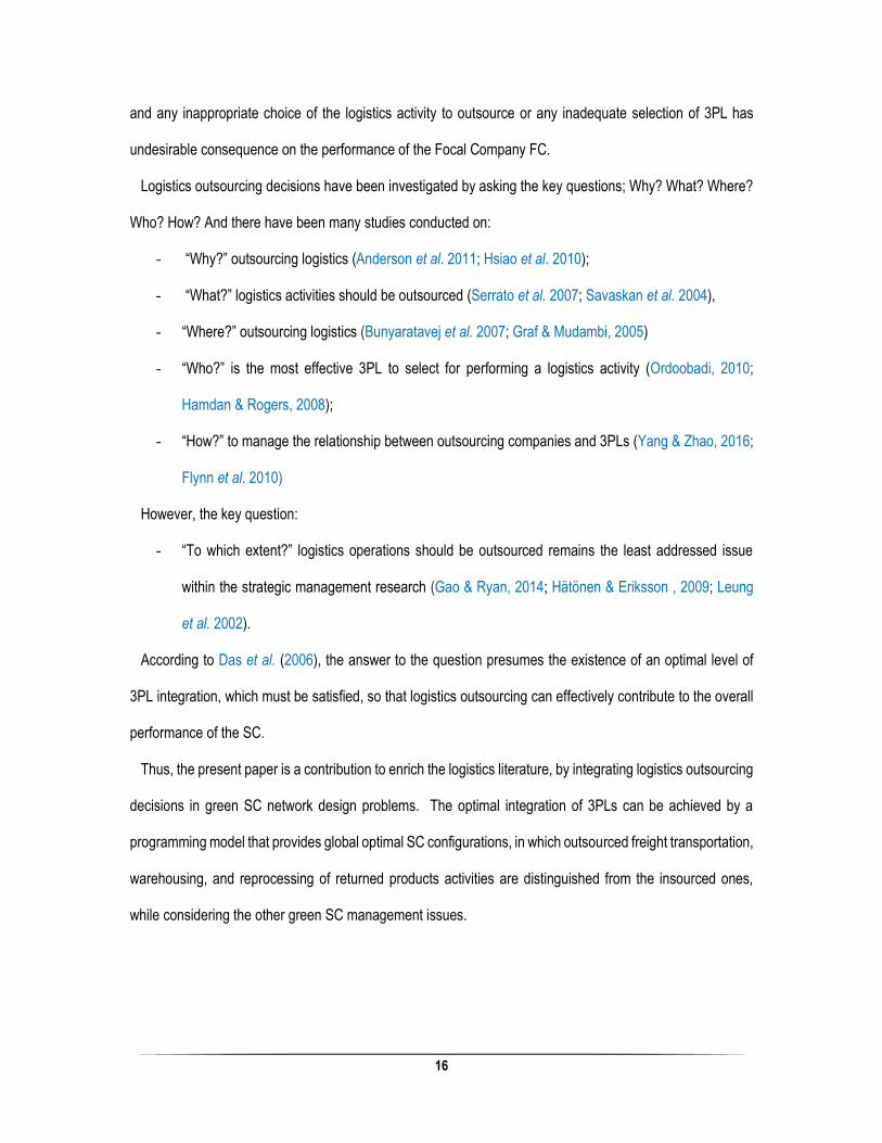
Logistics outsourcing decisions have been investigated by asking the key questions; Why? What? Where?
Who? How? And there have been many studies conducted on:
- “Why?” outsourcing logistics (Anderson et al. 2011; Hsiao et al. 2010);
- “What?” logistics activities should be outsourced (Serrato et al. 2007; Savaskan et al. 2004),
- “Where?” outsourcing logistics (Bunyaratavej et al. 2007; Graf & Mudambi, 2005)
- “Who?” is the most effective 3PL to select for performing a logistics activity (Ordoobadi, 2010;
Hamdan & Rogers, 2008);
- “How?” to manage the relationship between outsourcing companies and 3PLs (Yang & Zhao, 2016;
Flynn et al. 2010)
However, the key question:
- “To which extent?” logistics operations should be outsourced remains the least addressed issue
within the strategic management research (Gao & Ryan, 2014; Hätönen & Eriksson , 2009; Leung
et al. 2002).
According to Das et al. (2006), the answer to the question presumes the existence of an optimal level of
3PL integration, which must be satisfied, so that logistics outsourcing can effectively contribute to the overall
performance of the SC.
Thus, the present paper is a contribution to enrich the logistics literature, by integrating logistics outsourcing
decisions in green SC network design problems. The optimal integration of 3PLs can be achieved by a
programming model that provides global optimal SC configurations, in which outsourced freight transportation,
warehousing, and reprocessing of returned products activities are distinguished from the insourced ones,
while considering the other green SC management issues.
17
2.2.2. Green SC network design problem
The SC network design consists of combining SC management paradigms with Operational
Research models to optimize one or many objectives assigned to the SC. It determines a portfolio
of configuration parameters including the number, location, capacity, and type of various facilities in
the network (Wang et al. 2011). ‘‘Green’’ SC management refers to the way in which organizational
innovations and policies in SC management may be considered in the context of the sustainable
environment, and it involves different multiple objectives of social, economic and environmental
sustainability (Allaoui & Goncalves, 2013).
Many efforts have been made on the design of Green SC networks. The suggested models in the
literature can be classified according to four degrees of:
1) Scope; 2) Realism; 3) Complexity; and 4) Resolution:
- Scope: Forward (Nouira et al. 2016), reverse logistics (Demirel, & Gökçen, 2008), and
closed-loop SC networks (Pishvaee et al. 2010)
- Realism: Products/Customer segmentation (Salema et al. 2006); Time horizon (El-Sayed et
al. 2010), Regulation (Hoen et al. 2014; Fareeduddin et al. 2015); Supply security (Mirzapour
Al-e-hashem et al. 2013); and Outsourcing (Min & Ko, 2008).
- Complexity: Non-linear/Linear model programming (Wang et al. 2011); Multi-objective
(Ramezani et al. 2013); Stochastic (Pishvaee et al. 2009); and Robust (Gao & Ryan, 2014).
- Resolution: Classical methods such as parametrized objectives sum (Sazvar et al. 2014),
and epsilon-constraint method (Wang et al. 2011); and Non classical methods such as
evolutionary algorithms (Aravendan & Panneerselvam, 2015)
Ultimately, very few programming models have been proposed with high degrees of: 1) the scope
(e.g. limited echelons, forward or reverse logistics); 2) realism (e.g. some of SC management are

18
only considered, one period in the horizon time); 3) complexity (e. g. one objective to optimize,
deterministic or some of stochastic parameters); and 4) resolution (simplified examples to run the
programming models). For instance, many models are so far from the reality by neglecting or
mitigating the degree of those aspects. In their robust model, Gao & Ryan, (2014), highlighted the
importance to integrate the logistics outsourcing decisions within the SC network design problems,
to reduce business environment risks, and avoid sub-optimal SC configurations.
In this paper we try to capture the potential drawbacks (e.g. low degrees of the scope, realism,
complexity, and resolution) that repel the SC design models from the reality, and present a Bi-
objective, stochastic, multi-period, multi-product, multi-echelon programming model, which
integrates transportation, warehousing, and reprocessing of returned products outsourcing
decisions. The non-linear programming model has two objectives: minimizing both the expected
logistics cost, and the expected GHG emissions, in the context of business uncertainty. It considers
the Kraljic Portfolio Purchasing frame (Kraljic, 1983) for maximizing supply security and reducing
costs, considers the product/customer segmentation (Lee, 2002) for meeting the heterogeneous
requirements, and considers the Extended Producer Responsibility for managing effectively the End
of Life phase of products (Lindhqvist, 2000).
Hereunder, we define the closed-loop SC design problem, provide the SC designers with
constructive models to roughly estimate different costs of Insourced/Outsourced freight
transportation, warehousing, and reprocessing of returned products, and the corresponding GHG
emissions. Then, we present the modelling and solving approaches of the SC network design
problem.

19
2.3. Problem definition
2.3.1. General structure of the Closed-loop SC
The SC considered in this paper is an integrated forward/reverse logistics network, which organizes the
upstream and downstream into specific subnetworks, according to the characteristics of supplies, the
ownership of facilities, and the segmentation of deliveries and pickups. It is structured into 6 echelons:
- Echelon1: Referring to the Bill of Materials (BOM), raw materials, components, packages, and
accessories required to manufacture different products are categorized into four types of supplies
(sS). These supplies are managed with distinctive procurement strategies, to minimize cost and
maximize the supply security. According to Kraljic (1983), we distinguish: Noncritical supplies (s1),
which may be put together in large quantities, to optimize the order volume and inventory; Leverage
supplies (s2), which require competitive bidding and short term contracts to manage costs and
material flow; Bottleneck supplies (s3), which require keeping safety stock, and managing costs; and
Strategic supplies (s4), which require maintaining mutual trust, and open exchange of information to
ensure long-term availability. In this paper, the potential suppliers (nN) of each category of
supplies (s) are constrained to not exceed a maximum quota λs .
- Echelon 2: the FC operates a set M of plants (indexed mM), with assembly-type operations. The
supplies s S are transformed into three finished products (pP): Standard (p=1), Innovative (p=2),
and Hybrid (p=3). According to Vonderembse et al. (2006), p=1 are characterized by a steady
demand, and the customer contact tends to be periodic, rather than continuous; p=2 are designed
to be adaptable to changing customers’ requirements. They necessitate a close and continuous
customer contact, and have uncertain demands; and p=3 are complex products, which have several
components. They are supposed being the major purchases made periodically by the customers.
We suppose that any product (pP) is manufactured in a plant (mM), with respect to a

20
predetermined quota κpm , and the plants receive the recoverable products from potential
reprocessing centers, with the same quota.
- Echelon 3: A set of potential warehouses W (indexed wW) managed by FC, and a set of
warehouses V (indexed vV) managed by 3PLs, with known locations, and flexible annual
capacities are intended to streamline the flow of products (pP), between plants(mM) and
customer zones kK.
- Echelon 4: Considering simultaneously the behavior of demands and the characteristics of
customers, and according to Lee (2002), the distribution subnetwork is divided into four segments
(indexed iI), to satisfy the heterogeneous customer needs ; Cost-effective segment (i=1) which
aims for highest capacity utilization to create the cost efficiency in the SC; Responsive segment (i=2)
which follows an aggressive make-to-order strategy to be responsive, and flexible to changing
orders; Accurate segment (i=3) which strives to optimize inventories by keeping the pipeline flowing,
to reduce the risk of supply shortage; and Agile segment (i=4) which pursues a combination of make-
to-order and make-to- buffer stock strategies to be responsive, while reducing the risk of supply
shortage. The dynamic distribution of each segment may be characterized by a specific composition
of the demand, and a specific customer visiting frequency. This must have a significant effect on the
Inventory Turnover Rate ITRp of each product (pP) within the warehouses (wW) and (vV)
- Echelon 5: A substantial return flow of used products may result from either generous return policies
of the FC, or the Extended Producer Responsibility legislation. Collection centers (uU) belonging
to 3PLs, and potential hybrid warehouses (wW) managed by FC, with flexible subscribed
capacities are intended receiving and reprocessing a part of the returns from the distribution
segments (iI). We suppose that the recoverable products (pP) within the reprocessing centers
have the same ITR .
- Echelon 6: A fraction eDp of returned product (pP) is considered as an unrecoverable (scrapped)
product, and has to be shipped to disposal centers (indexed zZ) belonging to 3PLs, to continue

21
further recycling processes by means of others recyclers (out of the scope of this SC). The rest of
returned product (pP) is considered as a recoverable product, and has to be shipped to plants (m
M), for the purpose of remanufacturing.
We suppose in this paper, that there is no flow between the same nodes of a given echelon of the SC. The
general structure of the SC is illustrated in the figure 2.1.
The transportation, warehousing, and reprocessing activities may be performed by either the FC, or the
3PLs, depending on the optimal configurations of the SC network.
Hereunder, we provide constructive models for computing logistics costs and corresponding GHG emissions
of operating privately, or outsourcing the logistics operations.
Fig. 2.1. The general structure of the closed-loop Supply Chain

22
2.3.2. Logistics costs and GHG emissions computing models
It is not so easy to compare the economic and environmental performances of the FC as a private logistics
operator, and the 3PL service providers. But there are some basic assumptions that can be made, to structure
logistics costs and GHG emissions that FC and 3PL may experience. We suppose that we examine the nearly
identical available technologies, which are utilized in transportation, warehousing, and reprocessing of
discrete non-perishable products.
The structures of the logistics cost and GHG emissions depend on the volume performed, and the asset
ownership status of the facilities. According to Schniederjans et al. (2015), the ownership status may be as
follows:
- An external company supplies the asset with a subscribed capacity, but the management remains
with the FC (e.g. operating lease);
- A 3PL is contracted to supply and manage the assets (Logistics outsourcing); and
- The assets are owned by the FC, and a 3PL undertakes the management of the assets.
The present paper compares only the two first asset ownership statutes. Transportation, warehousing, and
reprocessing of used products, for the purpose of remanufacturing are question of in-sourcing or outsourcing,
but the disposal operation, is supposed to be outsourced, as being a special activity, which deals with recycling
operations of a great volume of raw materials.
2.3.2.1 Logistics cost computing models:
Logistics cost FCCost(X) = Freight transportation cost
+ Warehousing cost
+ Reprocessing cost
of returned product
+ Disposal cost
In the case of operating privately a logistics activity X, each entity of the cost may be divided into two parts:
fixed cost, and variable cost.
fCost(X)FCCost(X vcX
)= + .q(X) (i)

23
fCost(X) : Annual fixed cost to perform the activity X
vc :X Unit variable cost to perform the activity X, in terms of ($/unit of product)
Cap(X) :
The maximal number of product that may be performed annually by the activity X
(Subscribed capacity of X)
q(X) : The annual quantity processed by the activity X in terms of performed units of product
In the case of outsourcing the activity X to a 3PL, an according to Facanha & Horvath, (2005), and
Webster & Mitra, (2007) the fixed cost is transformed to a variable cost, and the cost of outsourcing may be
expressed as:
fCost(X)
3PLCost(X)=
(1+ ).(1- ). +3PL
π E .q(X)Cap( )
vcX X XX
(ii)
3PLπ :X
The profit margin of the 3PL service provider to perform the activity X.
E :X The efficiency of outsourcing the activity X.
0.05 E 0.20Transport
0.05 E 0.20Warehousing
0.10 E 0.10Reprocessing
Hereunder, we estimate the terms fCost(X) & vcXof each logistics operation X:
X: Freight transportation T
To determine fCostT and vcT
, three strategic issues should be addressed (Hoff et al. 2010; Zak et al.
2008): 1) Selecting the mode of transport, 2) Defining the fleet configuration (size of containers, trailers, and
trucks); and 3) Sizing the fleet & optimizing transportation routes.
1) Regarding the modalities, the scope of this paper is road-based and maritime freight transportation.
2) Concerning the fleet configuration, and according with Gencer et al. (2006), we use the principle of
first clustering around a given destination node within the network, second sizing the fleet. Land
origins are categorized into clusters. For instance, suppliers are categorized into strategic, leverage,
bottleneck, and critical clusters. Warehouses are categorized into warehouses belonging to FC, and
warehouses belonging to 3PL. Customers are categorized into cost-effective, responsive, accurate,

24
and agile segments, and reprocessing centers are categorized into hybrid warehouses belonging to
FC, and collection centers belonging to 3PL. Each cluster is divided into inside cluster, and outside
cluster, according to the geographic location, and we assign a fleet for each of them. To take
economics advantages of the larger vehicles over the longer distances, we suggest the following
configuration:
- If the average distance between the cluster of land origins and the land destination is δ 500 miles
( 804.64 km), then the FC will privately operate Medium Duty Vehicles MDV (e.g. Tractor-28 feet
trailer).
- Otherwise, the FC will operate Heavy Duty Vehicle HDV e.g. Tractor-53 feet trailer).
The FC should consider the strategic choice between leasing and privately managing the fleet, or
outsourcing it to a LTL (Less Than Truck Load) carrier for the short haul, and to a TL (Truck Load) carrier for
the long haul (Simchi-Levi et al. 2003).
When it is question to use maritime transportation, we suggest the use of 20 feet containers to load products
in a ship. The maritime operations may be privately managed or let it to a 3PL.
3) Concerning the fleet sizing, determining the right number of trucks for each configuration will depend
on several operational factors (Żak et al. 2008; McKinnon & Ge, 2006). Such as: Design of product;
Vehicle load factor; Speed; Vehicle reliability; Time of loading; Time of unloading; Rate of empty
running at each level of the SC; Amount of slack in deliveries or pick-up’s schedule, for managing
backloads; and Geographical variabilities.
In this paper, we are concerned by SC network Design problem, rather than Fleet Sizing & Vehicle Routing
problems. From the strategic perspective, we think that the first type of design problem must be talked in first,
and tactically, should be followed by the second type to capture all the operational factors. We refer the reader
to (Hoff et al. 2010), for details on fleet composition and routing.
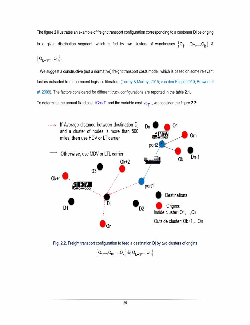
25
The figure 2 illustrates an example of freight transport configuration corresponding to a customer Dj belonging
to a given distribution segment, which is fed by two clusters of warehouses O ,...,O ,...,Om k1 &
O ,...,Onk+1.
We suggest a constructive (not a normative) freight transport costs model, which is based on some relevant
factors extracted from the recent logistics literature (Torrey & Murray, 2015; van den Engel, 2010; Browne et
al. 2009). The factors considered for different truck configurations are reported in the table 2.1.
To determine the annual fixed cost fCostT and the variable cost vcT
, we consider the figure 2.2:
Fig. 2.2. Freight transport configuration to feed a destination Dj by two clusters of origins
O ,...,O ,...,Om k1& O ,...,Onk+1

26
Table 2.1
Fixed cost & variable cost of truck configurations:
Region ε
Empty run rate
Type of
truck
Average Speed
(km/ hour)
Annual fixed cost
($)
Variable cost
($/TEU. Km)
North
America
0.16 to 0.18 HDV 64.0
42 762 0.32
MDV 45 483 0.14
Europe 0.28 to
0.24
HDV 50.6 14 000 0.59
MDV 14 900 0.68
(*) TEU: Twenty-foot Equivalent Unit container (20x8x8 feet)
Suppose that the destination Dj expects for an annual demand p
dDj
. A fraction β of the demand is projected
to be sourced from the outside cluster O ,...,O ,...,Om k1, and the remainder (1- β) from the inside cluster
O ,...,Onk+1.
TripOm,Dj
: The trip between the origin (Om) and the destination (Dj).
Trip = Trip + Trip + TripOm,Dj Om,port2 port2,port1 Port1,Dj
fCostTOm,D
CostT = + vCostTOm,Dj Oj m,Dj
** fCostTOm,Dj
is the total fixed cost of the fleet assigned to move annually all the products p from the
origin Om to the destination Dj.
** vCostTOm,Dj
is the total variable cost incurred to transport the volume pqOm,Djp
of products p
from Om to Dj.
Om= fCostT + fCostT
DjOm,pfCostT
ort2 porD t1,Om, j
fc .truck2=
p +fc .tr
Om,port2Np,truck2
fCostTOm,Dj Om/port1,DjN
p,uck truc 11 k

27
Om,port2N :
p,truck2
Number of trucks with capacity pcap
truck2 required to move the
expected demand β p
.dk Dj
of a product p, from the origin Om to the
destination Dj, during the effective annual time Teff
.
Om/port1-2,DjN :
p,truck1 Number of trucks with capacity p
captruck1
required to move the expected
demand
β+ (1- β)
k p.d
Djn
of a product p from the origin Om belonging
to the cluster outside, via the ports 1&2 to the destination Dj, during the
effective annual time Teff
Teff
= (2/3) Shift. (24) Hours/day. (5/7) days. (365) days/year
= 4 171.4 Hours/year
fctruck2
&fctruck1
:
Respectively are the fixed cost to operate annually the full capacity of
truck2, and truck1 (See the table 2.1)
=
β.fctruck2
k
1 p.d
βDj
+(1-β)pk
+ .fctr
fCostTOm,Dj
TTrip2
pcap
truck2
Teff Ttrip1
pcap
truck1
uck1n
(i,1)
= TimeTTrip Trip
= t (Load) + t (Transport) + t (Unload)
The time of waiting is not considered in this paper.
δ2t = (1+ ε2)
TransportOm,port2 v2; is the average time to perform the land trip from Om to the port2,
with a standard speed v2, by considering a rate of empty running ε2 , which depends on the geographic
area, and the nature of distribution (sourcing, inbound, outbound, or reverse logistics).
See table 1
δ1t = (1+ ε1)
TransportOm/port1,port2 v1; is the average time to perform the land trip from the port1 to
the destination Dj, with a standard speed v1, by considering a rate of empty running ε1

28
nδ + δport2,D Oi,Dδk port2,Oi i=k+1δ = & δ =
2 1 n-k+1ki=1
δ2
: Average distance between port 2, and origins Oi (i=1 to k)
δ1
: Average distance between the destination Dj, and origins Oi (i = (k+1) to n), plus port 1
Concerning the variable cost of transportation;
pvcTOm,
pvCostT = .qO Dm,D Omp
, where
p p p= vc + vc + vc
T TTOm,port2 port1,Dport2,port1
pvc
TOm,D
p pvc = vc .
T Truckδ .weightpOm,p2
Om,ort
22
port
p pvc = vc .
T Truckδ .weightpport1
po D1,D
rt1,
pvc =
Tport2,port1
vcseapYC20
pvc &
truck2p
vc :truck1
Respectively, unit variable cost of transporting privately a ton of product p for one
kilometer, in the truck2 with capacity pcap
truck2 ( p
captruck1
),
pq
Om : Annual units of product p, moved from the origin Om to the destination Dj, via the ports2-
1,
pY :C20
Total units of product p, which may be loaded in the container (20x8x8 feet) for shipping
vcsea : Variable cost for privately managing the maritime transport of a TEU (*) of product, from
one port to another.
weightp : Weight in ton of a unit of product p
For instance:
(*)vc = ($)1400 / TEU , in 56 hours
Qindao,Vancouver
(*)vc = ($) 2000 / TEU , in 64 hours Rotterdam,NewYork
(*) TEU: Twenty‐foot Equivalent Unit container (20x8x8 feet)
The Unit variable cost of transportation is:

29
=
vcp sea vc . +
truck2 .weightp
p
pvc
TOm,D
δpOm,port2
YC20
δpo
+vc .
truckD
1rt1,
(i,2)
X: Warehousing
The FC has to decide between leasing and managing a set of warehouses with flexible capacities, and
outsourcing the warehousing operation. In this paper, we consider the conventional rectangular
warehouses, which are often used in practice (Grosse & Glock, 2015). They consist of several parallel aisles;
front and back access aisles, and a depot in the front aisle. Products are assigned to storage locations based
on the demand frequencies of the products. So, the standard products p1 with the highest demand frequencies
are stored in the aisles closest to the depot, followed by hybrid products p3 in aisles with a medium distance
from the depot. Innovative products p2 with low demand frequencies are stored in the aisles farthest from the
depot.
To estimate the warehousing costs, the following assumptions are considered:
- Discrete non-perishable products p;
- 100% pallet in and 100% out, and only standard pallet is used (40’’x 48’’ = 3 1/3 ft. × 4ft);
- Pallets stored three high;
- All inbound and outbound are via truck load;
- Productivity labor εLabor
assumed equal to 25 pallets/ hour inbound, 25 pallets/ hour outbound;
- Only 70% of the warehouse space can be used to store products; and
- Electrical forklifts are only used to handle materials in the warehouse.
** The fixed cost fCostWw of a warehouse w=
Cost of leasing warehouse NNN (triple Net: N-property tax; N-insurance; & N-Maintenance) + Cost of
leasing “electrical” forklifts;

30
The cost of leasing warehouse NNN = ($ 5, 5 / square foot per year) * Ωw ;
Where
Ω :w : The squared feet facility w, which is proportional to the maximum of product units to store in
the warehouse w (subscribed capacity of warehousing Cappwp ). It depends on the staking
mode (e.g. Pallet three high), the number of items per pallet Np , and the dimensions of the
used pallet (e.g. Standard pallet: 40’’x 48’’).
Cappw2 2Ω (ft ) = . 13,331 (ft ).w 3
,3Np p
So, Cost of leasing warehouse NNN ($) = Cappw
31,79($).p Np
Cost of leasing “electrical” forklifts = ($ 750/ forklift/ month) * (12 months) * NFL
N :FL
Number of electrical forklifts required for processing goods. It depends and the capacity of
warehousing, the Inventory Turnover Rate of each product ITRp , the mode of staking, the
productivity of labor, and the effective time of warehousing.
Cap .ITRpw p2.
ε p NLabor pN =
FL 7(hours / days).2shifts.5(days / week).52weeks
So, fixed cost of warehousing is:
=
31,79($)+0,1978(
fCostW
$).ITRp
C
p
w
appw
p N
(i,3)
** The variable cost vCostWw of the warehouse w is:
vcW
vCostW = .p
qw pwp , where
q :pw Annual units of product p processed in the warehouse w;
vc :Wp
Variable cost for privately processing a unit of product p in any warehouse w
υLaborvc = εWp Laborp
, where

31
υ :Labor
Fully loaded hourly cost per warehouse worker: (includes, clerical, supervision, energy,
etc.)
υ = 2,5.Direct labor hourly rateLabor
2, 5. ($)15, 20 / hour = $3υLabor
8 / hour
ε :Labor
Productivity Labor
2. 38($/hour) 3,04= = ($ /unit)
25(pallet/hour).N Np p
vcWp
(i,4)
X: Reprocessing returns of products
In Baker & Canessa (2009), a distribution center design should be centred on the value-added operations,
storage and handling equipment, and that the building should then be designed around these. Reprocessing
the returns of products for remanufacturing consists of a series of operations. This, involves an additional
fixed cost in terms of space, materials handling, and equipment (e.g. Gravity roller conveyor; Trans-pallet;
oscilloscope, electrical screwdrivers, penetrating oil to loosen screws, etc.), and involves a variable cost in
terms of work force performing operations, within an expected processing time tCycle
per item.
According to Baker & Canessa (2009), the additional space required in a potential hybrid warehouse w may
be divided into two areas: One for sorting product returns (e.g. assembled products), and the other for storing
both the input, recoverable and unrecoverable products;
The space of reprocessing may be designed as a flexible number of workstations, with a “U” shaped layout
(Grosse & Glock, 2015), and a square footR
Ωw
per single workstation, operating two shifts per day. The figure
2.3 illustrates the workstation as follows:

32
Fig.2.3. ‘U’ shaped layout work station for reprocessing a returned product
The annual number of items which may be reprocessed in a single workstation is:
2(shifts).7(hours).5(days/week).52weeks 3640=t (hour) t (hour)Cycle Cycle
;
So the required number of workstations is
t . CapRCycle pwp
3640
, and the required surface is
t . CapRCycle pwpR
Ω . (feet)3640w
, where CapRpwp is the subscribed annual capacity of the returns
products p to be reprocessed in the hybrid warehouse w.
The space required for storing returned products may be determined like the case of warehousing, by the
formula:
CapRpw' 2Ω (ft ) 5,78.
w p N .ITRp
;
ITR : Average of Inventory Turnover Product of the returned products.
The number of electrical forklifts required for reprocessing product returns is
CapRpw2.
εLabor p Np'N =
FL 7(hours / days).2shifts.5(days / week).52weeks

33
** The fixed cost of reprocessing is:
=
t31.79 1.09CycleR
5,5 .Ω . + + CapRpw
wp 3640 N .
fCostHWw
ITR Np p
(i,5)
** The Variable cost of reprocessing is:
vcH
RvCostHW = .qw pwWp
Rq :pw
Annual units of returned product p reprocessed in the hybrid warehouse w;
vc :HW
Unit Variable cost for privately reprocessing the product p in any hybrid warehouse w
υ 38($/hour)Laborvc = =r rHW ε εLabor Labor
, where
rε :Labor
A productivity labor in reprocessing, which depends on the tCycle
2,5.15,2($ / hour)
= = 38.t .($ / unit)Cycle
1/ t (hour)Cycle
vcHW
(i,6)
2.3.2.2. Logistics GHG emissions computing models:
The GHG Protocol Corporate Standard provides a guidance for companies to prepare their GHG emissions
inventories, and seven GHG are covered by the Kyoto Protocol (WRI/WBCSD, 2004):
Carbon dioxide (CO2); Methane (CH4); Nitrous oxide (N2O); Hydro-fluorocarbons (HFCs);
Per-fluorocarbons (PFCs); Sulphur hexafluoride (SF6); and Nitrogen tri-fluoride (NF3).
In this paper, we consider only the most measurable GHG: CO2 with the reactive factor (Global Warming
Potential) GWP=1; CH4 with GWP=25; N2O with GWP=298; and HCF, especially CH2FCF3 (R 134a), with
GWP= 1430.
There are basically two approaches, to determine GHG emissions of logistics operations: The energy-based
approach, and the activity-based approach (McKinnon & Piecyk, 2011).
In the first approach, energy used in logistics activities is recorded, and standard emission factors are
employed to convert energy value into carbon equivalent emissions. In the case of energy data absence, it is

34
possible to make a rough estimate of the default factors of GHG emissions, by applying the second approach.
In the second vein, we determine the default factors of GHG emissions presented in
the table 2.2, by considering the following assumptions:
- The refrigerant R134a is used in the refrigeration system of tractors (not the trailers), with a quantity
of 3, 43 kg for MDV (28-foot), and 4, 28 kg for HDV (53-foot)), and the annual evaporative leakage
rate is about 25% (Tunnell, & Fender, 2010);
- The Energy consumption of Air conditioning of a warehouse is estimated to an average of
22 Btu / ft2, which represents about 8% of the total electricity consumption; according to U. S. Energy
Information Administration & CBECS (2003);
- The emissions & Generation Resource Integrated Database (eGRID), and non-eGRID average
emission factors for U.S. Electricity Use are: 1367 lbs CO2 / GWh; 20 lbs N2O / GWh; and 47 lbs
CH4 / GWh (Tunnell, & Fender, 2010).
- The amount of GHG emission resulting from disposal of one kilogram may be extracted from
references such as http://www.rcbc.ca/files/u3/ICF-final-report.pdf (refer to page 95, microwave oven
is taken as example in the table 2.2); and
- The warehouses, and collection centres use standard pallets (3 1/3 ft. × 4ft.), which are stored in
three high.
By analogy with the cost formulas, the GHG emissions amount of a logistics operation X may be expressed
as:
FCCO2(X)= (fe veX)+ .X
q(X) (iii)
fe(X) : Fixed amount of GHG emissions coming from the private physical asset of X, during one
year
:veX Variable amount of GHG emission coming from the combustion of fuel, or the production of
electricity, which are used in activity X, to privately operate a unit of product p.

35
X: Transportation:
pfeT vcOm,Dj TOm
pFCCO2T = + .qOm,Dj O, j mDp
=
β.fctruck2
k
1 p.d
βDj
+(1-β)pk
+ .fctruck1
feTOm,Dj
TTrip2
pcap
truck2
Teff Ttrip1
pcap
truck1
n
(iii,1)
.δOm,port2
= weight . +p p
Y
vCO2truck2
vCO2p maritime
veTOm,Dj
vCO2truc
.weightpC20
+ .δport1,Djk1
(iii,2)
fCO2 &truck1
fCO2truck2
Respectively, are the annual evaporative fluorocarbon emission (Ton EqCO2), coming
from the refrigeration of the truck 1 (truck2)
vCO2 &truck1
vCO2truck2
Respectively, are the unit variable emissions of CO2, CH4, and N2O emissions
coming from the combustion fuel in truck 1 (truck2) to move one ton of any product,
for one kilometer.
vCO2sea Unit variable emissions of CO2, CH4, and N2O emissions coming from the combustion
fuel in vessel to move 1 TEU, between two ports.
X: Warehousing
fe veW
FCW
CO2W = +w pqpwp
-6
3.1,688.10 .0,08(tonCO2eq) 5,78= . .Cap
pw13,33 N
e
pp
fW
(iii, 3)
3. (tonCO2) 5,78 2= . (ft )
2N13
-61,688.10 .0,92
veWp
,33(ft ) p
(iii, 4)

36
X: Reprocessing returns of products:
fe veHW
FCH
CO2HW = + qWpw pwp
(tonCO2eq)
= .CapRtCycle 5,78 pwRΩ . +p
3640
-60,030384.1
N .ITRw p
0
feHW
.
(iii, 5)
3. (tonCO2) 5,78 2= . (ft )
2N13.33(ft
-61,688.10 .0,92
ve
p
HWp)
(iii, 6)
In the case of outsourcing logistics activities to 3PL, and according to the research of MIT Center for
Transportation & Logistics (Blanco & Craig, 2009), a significant GHG emission inefficiency of 20 to 30% can
be observed by outsourcing operations:
Concerning the freight transportation, and comparing the network configuration of the focal company FC
and the 3PL, the 3PL tend to use a flexible routing network strategy, rather than a point-to-point strategy, to
consolidate the freight of different customers (Hesse & Rodrigue, 2004). This can generate a lot of stops
between different origins and destinations, hardly avoid traffic congestion, increase the distances, and
therefore raise the GHG emissions, notably CO2, N2O, and CH4.
Concerning the warehousing and reprocessing operations, we suppose that:
The fixed GHG emissions are not affected by the asset ownership statute, and the FC are more efficient that
3PL to rationalize the energy utilization within warehouses by controlling the frequency of entrances and exits.
fCO2X+
(3PL)CO2X = .quantity(X)
.vCO2X3PLζ
X
(iv)
3PLζ :X
Adjustment factor of GHG emissions, relative to the logistics activity X
3PL1.20 ζ 1.30X

37
Table 2.2
Default GHG emissions factors collected from specialized documents:
ATRI: American Transportation Research Institute, 2010; U.S. Environmental Protection Agency, 2008; Clean Cargo /BSR, 2012.
Conversion: 1 km = 0. 6214 miles; 1lb = 0. 45359 kg; 1gallon = 3. 785412 liters; 1kWh= 3412. 1416 Btu
Default factors of GHG
emissions
Scope 1 (In-house)
Direct emissions
Scope 2 (In-house)
Indirect emissions
Scope 3 (Outsourcing)
Optional Indirect emissions
Transportation
Mobile fuel
combustion
CO2
+ N2O
+ CH4
MDV
In North America: 759. 70 g CO2Eq /
TEU. Km
Mobile fuel
combustible
CO2
+ N2O
+ CH4
LTL
964.80 g CO2Eq /
TEU. Km
In EU: 888. 85 g CO2Eq /
TEU. Km
TL
509.70 g CO2Eq /
TEU. Km
HDV
In North America: 401. 30 g CO2Eq /
TEU. Km
Sea transport
EU- North
America EC
75.9 g CO2Eq / TEU. Km
Asia- North
America WC
65.1 g CO2Eq /
TEU. Km
Refrigerant
usage (not reefer container)
HFCs: R134a
MDV
1226 kg CO2Eq /vehicle
Refrigerant
usage (not reefer container)
HFCs: R134a
LTL
1226 kg CO2Eq /vehicle
HDV
1530 kg CO2Eq /vehicle
TL
1530 kg CO2Eq /vehicle
Warehousing &
Reprocessing
Electricity usage
1.688 g
CO2Eq / stored pallet
Electricity usage +
2.110 g
CO2Eq / stored pallet
Disposal CO2 + N2O + CH4
2. 481 g
CO2Eq /Kg of discarded product

38
Table 2.3
Expected annual quantity of product returnRtbpk
from customer k, for each product p with a fraction of return rbp
, at period t (= 1 to 6), for scenario b
Year t Demand
( Rtbpk
) Expected return of product p
1 D1bpk
r Dbp 1bpk
2 D2bpk
1r D + r (1- r ) Dbp bp bp2bpk 1bpk
3 D3bpk
1 2r D + r (1- r ) D + r (1- r ) Dbp bp bp bp bp3bpk 2bpk 1bpk
4 D4bpk
1 2 3r D + r (1- r ) D + r (1- r ) D + r (1- r ) Dbp bp bp bp bp bp bp4bpk 3bpk 2bpk 1bpk
5 D5bpk
1 2 3 4r D + r (1- r ) D + r (1- r ) D + r (1- r ) D + r (1- r ) Dbp 5bpk bp bp bp bp bp bp bp bp4bpk 3bpk 2bpk 1bpk
6 D6bpk
1 2 3 4 5r D + r (1- r ) D + r (1- r ) D + r (1- r ) D + r (1- r ) D + r (1- r ) Dbp bp bp 5bpk bp bp bp bp bp bp bp bp6bpk 4bpk 3bpk 2bpk 1bpk

39
2.4. Modelling & Solving approaches
2.4.1. Problem formulation
During a set of periods T (indexed tT), the focal company FC, which controls the whole closed loop SC
described in the section 3, desires optimizing its SC, by minimizing two objective functions:
- Total expected logistics cost OBJ1 (1), and
- Total expected logistics GHG emissions OBJ2 (2).
** Objective functions:
OBJ1: minimize Z
Z: Expected total logistics cost ($ US)
Z = Z1+ Z2+ Z3+ Z4+ Z5+ Z6+ Z7+ Z8+ Z9 (1)
Z1: Freight transport cost from suppliers to plants
Z2: Freight transport cost from plants to warehouses
Z3: Freight transport cost from warehouses to customers’ zones
Z4: Freight transport cost from distribution segments to reprocessing centers (hybrid warehouses &
collection centers)
Z5: Freight transport cost of recoverable product from reprocessing centers to plants
Z6: Freight transport cost of unrecoverable product from reprocessing centers to disposal centers
Z7: Cost of Warehousing
Z8: Cost of Reprocessing
Z9: Cost of Disposal
See analytical expressions of Zi= 1, 6 in table 2.5, and
Zi=7, 9 in table 2.6.

40
OBJ2: minimize C
C = C1+ C2+ C3 (2)
C1: Direct CO2, N2O, CH4, HFC (R-143a) emissions from leased or purchased fleet operating within the
Closed loop-SC:
The Scope 1, according to The Greenhouse Gas Protocol (WRI & WBCSD, 2004).
C2: Indirect GHG emissions associated to the purchase and use of electricity within potential FC’s
warehouses & hybrid warehouses; The Scope 2, according to The Greenhouse Gas Protocol (WRI &
WBCSD, 2004).
C3: Indirect emissions associated to any outsourced logistics services; The Scope 3, according to The
Greenhouse Gas Protocol (WRI & WBCSD, 2004)
See analytical expressions of C1 and C2 in table 2.7, and C3 in table 2.8.
** Decision variables: Strategic, and tactical variables
The logistics activities are freight transportation, warehousing, reprocessing of product returns, and disposal
of unrecoverable products. These logistics activities are subject of total or partial outsourcing.
- Boolean decision variables (Strategic)
x :sm =1 if FC in-sources transportation of the category of supplies s, from corresponding
suppliers to plant m. Otherwise = 0;
x :w =1 if FC in-sources transportation of products, from any plant to the warehouse w.
Otherwise = 0;
x :v =1 if FC in-sources transportation of products, from any plant to the 3PL warehouse v.
Otherwise = 0;
x :Wk =1 if FC in-sources transportation of products, from any FC’s warehouse to the customer
zone k. Otherwise = 0;
x :Vk =1 if FC in-sources transportation of products, from any 3PL’s warehouse to the customer
zone k. Otherwise = 0;
x :iw
=1 if FC in-sources transportation of returned products, from the distribution segment i to
the FC’s warehouse w. Otherwise = 0;

41
x :iu =1 if FC in-sources transportation of returned products, from the distribution segment i to
3PL’s collection center u. Otherwise = 0;
x :HWm
=1 if FC in-sources transportation of recoverable products, from hybrid warehouses to the
plant m. Otherwise = 0;
x :Um =1 if FC in-sources transportation of recoverable products, from collection centers to the
plant m. Otherwise = 0;
x :HWz
=1 if FC in-sources transportation of unrecoverable products, from hybrid warehouses to
the 3PL’s disposal center z. Otherwise = 0;
x :Uz =1 if FC in-sources transportation of unrecoverable products, from collection centers to the
3PL’s disposal center z. Otherwise = 0;
y :w =1 if FC’s warehouse w is open. Otherwise = 0;
Y :w =1 if w is open as a hybrid warehouse. Otherwise = 0;
- Integer decision variables (Tactical)
q ;tbpsnm
q & q ;tbpmw tbpmv
q & q ;tbpwk tbpvk
q & q ;tbpkw tbpku
q & q ;tbpwm tbpum
q & qtbpwz tbpuz
Number of units of supplies, products, returns, recoverable products, and
unrecoverable products transported from the node i to node j of the SC, at a
period tT, and within scenario bB. Where;
sS; nN; pP; mM; wW; vV; kK; uU; & zZ.
The model has two types of parameters: Deterministic, and stochastic parameters.
** Deterministic Parameters:
h : Rate of inflation
λ :s Maximum fraction of supply s, which can be purchased from a supplier (e. g.
Security of supply)
κ :pm Quota of manufacturing and remanufacturing the product p in the plant m (e. g.
Manufacturing strategy)
weight :p Weight of a unit of product p
weightR :p Weight of a unit of returned product p

42
weight :s Average weight of supply s required to manufacture a unit product,
ITR :p Inventory turnover rate of p in any warehouse (e.g. Standard, Innovative, and Hybrid
products)
ve :Tsnm
Variable GHG emissions in (Tons of CO2eq/Ton. Km) of transporting privately the
supplies required by plant m, from the corresponding supplier n,
ve :Tpmw
Variable GHG emissions in (Tons of CO2eq/Ton. Km) of transporting privately the
product p, from the plant m, to the warehouse w
ve :Tpmv
Variable GHG emissions in (Tons of CO2eq/Ton. Km) of transporting privately the
product p, from the plant m, to the warehouse v
ve :Tpwk
Variable GHG emissions in (Tons of CO2eq/Ton. Km) of transporting privately the
product p, from the warehouse w, to the customer zone k
ve :Tpvk
Variable GHG emissions in (Tons of CO2eq/Ton. Km) of transporting privately the
product p, from the warehouse v, to the customer zone k
ve :TR
pkw Variable GHG emissions in (Tons of CO2eq/Ton. Km) of transporting privately the
returned product p, from the customer zone k to the hybrid warehouse w
ve :TRpku
Variable GHG emissions in (Tons of CO2eq/Ton. Km) of transporting privately the
returned product p, from the customer zone k to the collection center u
ve :THWpwm
Variable GHG emissions in (Tons of CO2eq/Ton. Km) of transporting privately the
recoverable product p, from the hybrid warehouse w, to the plant m
ve :TUpum
Variable GHG emissions in (Tons of CO2eq/Ton. Km) of transporting privately the
recoverable product p, from the collection center u, to the plant m
ve :THWpwz
Variable GHG emissions in (Tons of CO2eq/Ton. Km) of transporting privately the
unrecoverable product p, from the hybrid warehouse w, to the disposal center z
ve :TUpuz
Variable GHG emissions in (Tons of CO2eq/Ton. Km) of transporting privately the
unrecoverable product p, from the collection center u, to the disposal center z
ve :Wpw
Variable GHG emissions in (Tons of CO2eq/Ton of product) of warehousing
privately the product p, in the warehouse w
ve :HWpw
Variable GHG emissions in (Tons of CO2eq/Ton of returned product) of
reprocessing privately the used product p, in the hybrid warehouse w
** Stochastic parameters:
To capture the uncertainty relative to: 1) demand of multi-product p; 2) extended capacities of facilities to
face demand; 2) quantity of product returns; 3) quality of product returns; and 4) different logistics variable

43
costs, a stochastic plan for a limited horizon of time T may be established by using a scenarios based
approach.
To do so, we suppose that the FC resorts to a strategic consulting to indorse or adapt the assumptions of
constructive models; and the deterministic parameters, and to model the behavior of uncertain parameters.
Drawing our inspiration from Serrato et al. (2007), we suppose that within a scenario b, the demand of
product p at the period t = 1 is D1bp
, and the amount of returns is r Dbp 1bp
, where rbp
is the average fraction
of product returns p corresponding to the current demand. The demand at t = 2 isD2bp
, but the amount of
returns will be r Dbp 2bp
+ r (1- r )Dbp bp 1bp
. The demand at t = 3 isD3bp
, but the amount of returns will be
r Dbp 3bp
+ 1
r (1- r ) Dbp bp 2bp
+2
r (1- r ) Dbp bp 1bp
, and so on (See the table 2.3).
Following Pishvaee et al. (2008), within a no long interval of time, say 6-10 years, all possible scenarios
describing the behaviour of uncertain parameters may be elaborated by means of semantic attribution (e. g.
High, Medium; Low). According to the strategic consulting group, expected annual values of the parameters
are adopted. These possible scenarios may be aggregated into a set of most probable scenarios B (indexed
bB), say 5-7 probable scenarios within the time interval. The dynamic change between scenarios needs to
be approached by a transition matrix, which “ideally” should be constant in time (Meyn & Tweedie, 1996). In
other words, the system of parameters is considered as a Markov chain, in which the future behaviour of the
system is determined only by its present state, and it is independent of the way in which this state has
developed. If not so, the stochastic plan may include more than one transition matrix switching between
themselves (Horn, 1975)
We basically consider the dynamic change of scenarios following a Markov Chain with one constant matrix
of transition. So, the marginal probabilities of scenarios at a given period t may be determined by the formula
Chapman-Kolmogorov (Ross, 2009). The table 2.4 gives an example of a stochastic plan relative to the
working case study of a FC which manufactures, distributes, and reprocesses three technologies of
microwave ovens.

44
Hereunder, we list the stochastic parameters:
prob :tb Marginal probability occurrence of the scenario b, at t.
fc &Ttbsm
fe :Ttbsm
Respectively, the annual fixed cost in ($) (GHG emissions in Tons of CO2eq) of
transporting privately the supplies s required by plant m, at period t for scenario b.
vc :Ttbsnm
Variable cost in ($/Ton of supply s) of transporting privately the supplies required by
plant m, from the corresponding supplier n, at period t for scenario b.
c &3PLTtbsnm
e3PLT :tbsnm
Respectively, the outsourcing cost in ($/Ton of supply s) (GHG emissions in Tons of
CO2eq/Ton. Km) of transporting the supplies required by plant m, from the
corresponding supplier n, at period t for scenario b.
fc &Ttbw
fe :Ttbw
Respectively, the annual fixed cost in ($) (GHG emissions in Tons of CO2eq) of
transporting privately products, from plants to the FC’s warehouse w, at period t for
scenario b.
vc :Ttbpmw
Variable cost in ($/Ton of product p) of transporting privately the product p, from the
plant m, to the warehouse w, at period t for scenario b.
c &3PLTtbpmw
e :3PLTtbpmw
Respectively, the outsourcing cost in ($/Ton of product p) (GHG emissions in Tons of
CO2eq/Ton. Km) of transporting the product p, from the plant m, to the warehouse w,
at period t for scenario b.
fc &Ttbv
fe :Ttbv
Respectively, the annual fixed cost in ($) (GHG emissions in Tons of CO2eq) of
transporting privately products, from plants to the 3PL’s warehouse v, at period t for
scenario b.
vc :Ttbpmv
Variable cost in ($/Ton of product p) of transporting privately the product p, from the
plant m, to the warehouse v, at period t for scenario b.
c &3PLTtbpmv
e :3PLTtbpmv
Respectively, the outsourcing cost in ($/Ton of product p) (GHG emissions in Tons of
CO2eq/Ton. Km) of transporting the product p, from the plant m, to the warehouse v, at
period t for scenario b.
fc &TW
t,b,k
fe :TW
t,b,k
Respectively, the annual fixed cost in ($) (GHG emissions in Tons of CO2eq) of
transporting privately products, from FC’s warehouses to the customer zone k, at period
t for scenario b.
fc &TV
t,b,k
fe :TV
t,b,k
Respectively, the annual fixed cost in ($) (GHG emissions in Tons of CO2eq) of
transporting privately products, from 3PL’s warehouses to the customer zone k, at
period t for scenario b.

45
vc :Ttbpwk
Variable cost in ($/Ton of product p) of transporting privately the product p, from the
warehouse w, to the customer zone k, at period t for scenario b.
vc :Ttbpvk
Variable cost in ($/Ton of product p) of transporting privately the product p, from the
warehouse v, to the customer zone k, at period t for scenario b.
c &3PLTtbpwk
e :3PLTtbpwk
Respectively, the outsourcing cost in ($/Ton of product p) (GHG emissions in Tons of
CO2eq/Ton. Km) of transporting the product p, from the warehouse w, to the customer
zone k, at period t for scenario b.
c &3PLTtbpvk
e :3PLTtbpvk
Respectively, the outsourcing cost in ($/Ton of product p) (GHG emissions in Tons of
CO2eq/Ton. Km) of transporting the product p, from the warehouse v, to the customer
zone k, at period t for scenario b.
fc &TR
tbiw
fe :TR
tbiw
Respectively, the annual fixed cost in ($) (GHG emissions in Tons of CO2eq) of
transporting privately the returned products, from the distribution segment i to the FC’s
hybrid warehouse w, at period t for scenario b.
fc &TR
tbiu
fe :TR
tbiu
Respectively, the annual fixed cost in ($) (GHG emissions in Tons of CO2eq) of
transporting privately the returned products, from the distribution segment i to the 3PL’s
collection center u, at period t for scenario b.
vc :TR
tbpkw Variable cost in ($/Ton of returned product p) of transporting privately the returned
product p, from the customer zone k to the hybrid warehouse w, at period t for scenario
b.
vc :TRtbpku
Variable cost in ($/Ton of returned product p) of transporting privately the returned
product p, from the customer zone k to the collection center u, to at period t for scenario
b.
c &3PLTRtbpkw
e :3PLTRtbpkw
Respectively, the outsourcing cost in ($/Ton of returned product p) (GHG emissions in
Tons of CO2eq/Ton. Km) of transporting the returned product p, from customer zone k
to the hybrid warehouse w, at period t for scenario b.
c &3PLTRtbpku
e :3PLTRtbpku
Respectively, the outsourcing cost in ($/Ton of returned product p) (GHG emissions in
Tons of CO2eq/Ton. Km) of transporting the returned product p, from customer zone k
to the collection center u, at period t for scenario b.
fc &THW
tbm
fe :THW
tbm
Respectively, the annual fixed cost in ($) (GHG emissions in Tons of CO2eq) of
transporting privately the recoverable products, from hybrid warehouses to the plant m,
at period t for scenario b.

46
fc &TU
tbm
fe :TU
tbm
Respectively, the annual fixed cost in ($) (GHG emissions in Tons of CO2eq) of
transporting privately the recoverable products, from collection centers to the plant m,
at period t for scenario b.
vc :THW
tbpwm Variable cost in ($/Ton of returned product p) of transporting privately the recoverable
product p, from the hybrid warehouse w, to the plant m, at period t for scenario b.
vc :TU
tbpum Variable cost in ($/Ton of returned product p) of transporting privately the recoverable
product p, from the collection center u, to the plant m, at period t for scenario b.
c &3PLTWHtbpwm
e :3PLTWHtbpwm
Respectively, the outsourcing cost in ($/Ton of returned product p) (GHG emissions in
Tons of CO2eq/Ton. Km) of transporting the recoverable product p, from the hybrid
warehouse w to the plant m, at period t for scenario b.
c &3PLTUtbpum
e :3PLTUtbpum
Respectively, the outsourcing cost in ($/Ton of returned product p) (GHG emissions in
Tons of CO2eq/Ton. Km) of transporting the recoverable product p, from the collection
center u to the plant m, at period t for scenario b.
fc &TU
tbz
fe :TU
tbz
Respectively, the annual fixed cost in ($) (GHG emissions in Tons of CO2eq) of
transporting privately the unrecoverable products, from collection centers to the 3PL’s
disposal center z, at period t for scenario b.
fc &THW
tbz
fe :THW
tbz
Respectively, the annual fixed cost in ($) (GHG emissions in Tons of CO2eq) of
transporting privately the unrecoverable products, from hybrid warehouses to the 3PL’s
disposal center z, at period t for scenario b.
vc :THWtbpwz
Variable cost in ($/Ton of returned product p) of transporting privately the unrecoverable
product p, from the hybrid warehouse w, to the disposal center z, at period t for scenario
b.
vc :TUtbpuz
Variable cost in ($/Ton of returned product p) of transporting privately the unrecoverable
product p, from the collection center u, to the disposal center z, at period t for scenario
b.
c &3PLTWHtbpwz
e :3PLTWHtbpwz
Respectively, the outsourcing cost in ($/Ton of returned product p) (GHG emissions in
Tons of CO2eq/Ton. Km) of transporting the unrecoverable product p, from the hybrid
warehouse w to the disposal center z, at period t for scenario b.
c &3PLTUtbpuz
e :3PLTUtbpuz
Respectively, the outsourcing cost in ($/Ton of returned product p) (GHG emissions in
Tons of CO2eq/Ton. Km) of transporting the unrecoverable product p, from the
collection center u to the disposal center z, at period t for scenario b.

47
fc &W
tbw
fe :W
tbw
Respectively, the annual fixed cost in ($) (GHG emissions in Tons of CO2eq) of
warehousing privately the products, in the warehouse w, at period t for scenario b.
vc :W
tbpw Variable GHG emissions in (Tons of CO2eq/Ton of product) of warehousing privately
the product p, in the warehouse w, at period t for scenario b.
3PLc &V
tbpv
3PLe :V
tbpv
Respectively, the outsourcing cost in ($/Ton of product p) (GHG emissions in Tons of
CO2eq/Ton of product) of warehousing the product p, in the warehouse v, at period t
for scenario b.
fc &HW
tbw
fe :HW
tbw
Respectively, the annual fixed cost in ($) (GHG emissions in Tons of CO2eq) of
reprocessing privately the returned products, in the hybrid warehouse w, at period t for
scenario b.
vc :HWtbpw
Variable cost in ($/Ton of returned product p) of reprocessing privately the returned
product p, in the hybrid warehouse w, at period t for scenario b.
3PLc &U
tbpu
3PLe :U
tbpu
Respectively, the outsourcing cost in ($/Ton of returned product p) (GHG emissions in
Tons of CO2eq/Ton. Km) of reprocessing the returned product p, in the collection center
u, at period t for scenario b.
3PLc &Z
tbz
3PLe :Z
tbz
Respectively, the outsourcing cost in ($/Ton of returned product p) (GHG emissions in
Tons of CO2eq/Ton. Km) to dispose of the returned product p, in the 3PL’s center z, at
period t for scenario b.
D :tbpk Demand of product of customer k, at period t for scenario b.
R :tbpk
Return of product from customer k, at period t for scenario b (see the table 2.3)
eD :bp
Average fraction of returned product p P which is considered as an unrecoverable
(scrapped) product, and has to be shipped to disposal centers, for a scenario b,
whatever the period
S :tbpsm
Expected annual units of supply s required to make the product p in the plant m, at
period t, for scenario b.
CapM :tbp Expected annual capacity of manufacturing the product p, at period t, for scenario b. It
depends on the expected annual demand.
CapW :tbpw Subscribed capacity of warehousing the product p, in the warehouse w, at period t, for
scenario b.

48
CapR :tbpw
Expected annual returns of product p to be reprocessed in the hybrid warehouse w, at
period t, for scenario b.
CapR :tbpu
Expected annual returns of product p to be reprocessed in the collection center u, at
period t, for scenario b.
CapD :tbz
Subscribed capacity to dispose of unrecoverable products, in the disposal center z, at
period t, for scenario b.
The two objective functions are subject to five types of constraints:
** Constraint flows (3-8); within any facility, the number of inputs is equal to the number of output.
** Capacity constraints (9-15); each facility should respect the annual subscribed capacity, before
planned.
** Opening constraints (16-20); no warehousing or reprocessing operation is privately performed in a
facility not open.
** Installation constraints (21-23); no product delivery is made to a non-open facility.
** Non-negative Integer (discrete products) & Binary constraints (strategic decision: 0 or 1) (24-25).
** Flow constraints:
(q + q ) = (q + q ); t, b, p, w, vtbpmw tbpwktbpmv tbpvkm k
(3)
q + q = D ; t, b, p, ktbpwk tbpvk tbpkw v
(4)
q + q = R ; t, b, p, ktbpkw tbpku tbpkw u
(5)
q + q = eD . R ; t,b,ptbpwz tbpuz tbpkbpw,z u,z k
(6)
q + q = (1- eD ). R ; t,b,ptbpwm tbpum tbpkbpw,m u,m k
(7)
q + q = κ .(1- eD ). R ; t,b,p,mtbpwm tbpum tbpkpm bpw u k
(8)
** Capacity constraints:
q λ S ; t,b,p,s,nstbpsnm tbpsm (9)
q + q κ .CapM ; t,b,p,mtbpmw tbpmv pm tbpw v
(10)
q ITR CapW ; t,b,p,wtbpmw p tbpwm
(11)

49
q ITR CapW ; t,b,p,vtbpmv p tbpvm
(12)
q CapR ; t,b,p,wtbpkw tbpwk
(13)
q CapR ; t,b,p,utbpku tbpuk
(14)
q + q CapD ; t,b,ztbpwz tbpuz tbzp,w p,u
(15)
** Opening constraints of warehouses:
L is a very large number
q L.y ; t,b,p,m,wwtbpmw (16)
q L.y ; t,b,p,k,wwtbpwk (17)
q L.Y ; t,b,p,k,wwtbpkw (18)
q L.Y ; t,b,p,m,wwtbpwm (19)
q L.Y ; t,b,p,z,wwtbpwz (20)
** Installation constraints:
Transportation to warehouses and to hybrid warehouses is possible only if they are opened, & Opening
the warehouses as hybrid facilities is possible, if they were already opened as conventional facilities:
x y ; ww w (21)
x Y ; i,wwiw (22)
x Y ; i,wwiw (23)
** Non-negative Integer, & Binary constraints:
x ,x ,x ,x ,x ,x ,x ,sm w v Wk Vk iw iu
x ,x ,x ,x ,y ,Y 0,1w wHWm Um HWz Uz
p, s, m, w, v, i, k, u, z
(24)
q ,q ,q ,q ,tbpsnm tbpmw tbpmv tbpwk
q ,q ,q ,q ,tbpvk tbpkw tbpku tbpwm
q ,q ,qtbpum tbpwz tbpuz
are non-negative integer numbers
t,b,s,p,n, m, w, v, k, u, z v
(25)
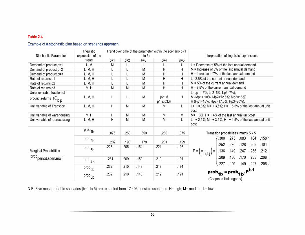
50
Table 2.4
Example of a stochastic plan based on scenarios approach
Stochastic Parameter
linguistic expression of the
trend
Trend over time of the parameter within the scenario b (1 to 5)
Interpretation of linguistic expressions
b=1 b=2 b=3 b=4 b=5
Demand of product p=1 L, M M L L L L L = Decrease of 5% of the last annual demand M = Increase of 3% of the last annual demand H = Increase of 7% of the last annual demand
Demand of product p=2 L, M, H L L M H H
Demand of product p=3 L, M, H L L M H H
Rate of returns p1 L, M, H L L M H H L =2.5% of the current annual demand M = 5% of the current annual demand H = 7.5% of the current annual demand
Rate of returns p2 L, M, H L L M H H
Rate of returns p3 M, H M M M H H
Unrecoverable fraction of
product returns eDb,p
L, M, H
L
L
M
p2: M
p1 & p3:H
H
L (Lp1= 5%; Lp2=6%; Lp3=7%); M (Mp1= 10%; Mp2=12.5%; Mp3=15%) H (Hp1=15%; Hp2=17.5%; Hp3=20%).
Unit variable of Transport L, M, H H M M M L L= + 0,8%; M= + 3,5%; H= + 5,5% of the last annual unit cost
Unit variable of warehousing M, H H M M M M M= + 3%, H= + 4% of the last annual unit cost
Unit variable of reprocessing L, M, H H M M M L L= + 2,5%; M= + 3,5%; H= + 4,5% of the last annual unit cost
Marginal Probabilities
probperiod,scenario
=
prob1b
.075
.250
.350
.250
.075
Transition probabilities’ matrix 5 x 5
.300 .275 .083 .184 .158
.252 .230 .128 .209 .181
P = π = .136 .149 .247 .256 .212bi,bj
.209 .180 .170 .233 .208
.227 .191 .149 .227 .206
t-1prob =prob .P
tb 1b
(Chapman-Kolmogorov)
prob2b
.202
.190
.178
.231
.199
prob3b
.226 .205 .154 .221 .193
prob4b
.231 .209 .150 .219 .191
prob5b
.232 .210 .149 .219 .191
prob6b
.232 .210 .148 .219 .191
N.B. Five most probable scenarios (b=1 to 5) are extracted from 17 496 possible scenarios. H= high; M= medium; L= low.

51
Table 2.5
Freight transportation costs expressions:
1Z =
tprob (1+ h) fc xsmtb Ttbsmt,b,s,m
+ prob weight δ vc x qs nm smtb tbpsnmTtbsnmt,b,p,s,n,m
weight δs nm+ prob q3PLtb tbpsnm.(1-x )csm Tt,b,p,s,n,m
tbsnm
(1.1)
1Z =
t tprob (1+h) fc x + prob (1+h) fc xw vtb T tb Tvtbwt,b,w t,b,v
+ prob weight δ vc x qp mw wtb tbpmwTtbpmwt,b,p,m,w
+ prob weight δ vc x qp mv vtb tbpmvTtbpmvt,b,p,m,v
weight δp mw+ prob 3PLtb (1-x )cpwt,b, Ttbpmw
qtbpmw
p,m,w
weight δp mv+ prob q3PLtb tbpmv(1-x )cpvt,b,p,m,v Ttbpmv
(1.2)
t tprob (1+h) fc x + prob (1+h) fc xtb TW Wk tb TV Vkk kt,b,k t,b,k
+ prob weight δ vc x qptb wk Wk tbpwkTtbpwkt,b,p,w,k
Z = + prob weight δ vc x qptb vk Vk tbpvk3 Ttbpvkt,b,p,v,k
3PL+ prob weight δ (1-x )cptb wk Wk Ttbpwkt,b,
qtbpwkp,w,k
3PL+ prob weight δ (1-x )c qptb vk Vk tbpvkTtbpvkt,b,p,v,k
(1.3)

52
4
t tprob (1+h) fc x + prob (1+h) fc xtb iw tb iuTR TRtbiw tbiut,b,i,w t,b,i,u
+ prob weightR δ vc x qptb wk iw tbpkwTRtbpkwt,b,p,w,i,k
Z = + prob weightR δ vc x qptb ku iu tbpkuTRtbpkut,b,p,u,i,k
weightR δ .(1-x )p wk iw+ probtb
q3PL tbpkw.ct,b,p,w,i,k TRtbpkw
weightR δ .(1-x )p ku iu+ prob q3PLtb tbpku.ct,b,p,u,i,k TRtbpku
(1.4)
t tprob (1+h) fc x + prob (1+h) fc xtb HWm tb UmTHW TUtbm tbmt,b,m t,b,m
+ prob weightR δ vc x qp mwtb HWm tbpwmTtbpwmt,b,p,m,w
Z = + prob weightR δ vc x qp mutb Um5 tbpumTtbpumt,b,p,m,u
weightR δp mw+ prob 3tb .(1-x )cHWm Ttbpwm
qPL tbpwmt,b,p,m,w
weightR δp mu+ prob q3PLtb tbpum.(1-x )cUmt,b,p,m,u Ttbpum
(1.5)
t tprob (1+h) fc x + prob (1+h) fc xtb HWz tb UzTHW TUtbz tbzt,b,z t,b,z
+ prob weightR δ vc x qp wztb HWz tbpwzTRtbpzwt,b,p,w,z
Z = + prob weightR δ vc x qp uztb Uz tbpuz6 TRtbpzut,b,p,u,z
+ prob weightR δ (1-x )cp wztb HWz Ttbpwz
3PL qtbpwzt,b,p,w,z
3PL+ prob weightR δ (1-x )c qp uztb Uz tbpuzTtbpuzt,b,p,u,z
(1.6)

53
Table 2.6
Warehousing, reprocessing, and disposal costs expressions:
tprob (1+h) fc ywtb Wtbwt,b,w
Z = + prob vc qtb tbpmw7 Wtbpwt,b,p,m,w
3PL+ prob c qtb tbpmvVtbpvt,b,p,m,v
(1.7)
tprob (1+h) fc Ywtb HWtbwt,b,w
Z = + prob vc qtb tbpkw8 HWtbpwt,b,p,k,w
3PL+ prob c qtb tbpkuUtbput,b,p,k,u
(1.8)
3PLprob c qtb tbpwzZtbzt,b,p,w,zZ =
9 3PL+ prob c qtb tbpuzZtbzt,b,p,u,z
(1.9)

54
Table 2.7
GHG emissions’ expressions (Scope1 & Scope2) :
C =1
(2.1)
prob fe xsmtb Ttbsmt,b,s,m
+ prob fe x + prob fe xw vtb tbT Ttbw tbvt,b,w t,b,v
+ prob fe x + prob fe xtb Wk tb VkTW TVtbk tbkt,b,k t,b,k
+ prob fe x + prob fe xtb iw tb iuTR TRtbiw tbiut,b,i,w t,b,i,u
+ prob fe x + prob fetb HWm tbTHW TUtbmt,b,m
xUmtbmt,b,m
+ prob fe x + prob fe xtb HWz tb UzTHW TUtbz tbzt,b,z t,b,z
+
weightS δps nmprob x qsmtb tbpnm.ve
Tt,b,p,s,n,m snm
weight δ weight δp mw p mv+ prob x q + prob x qw vtb tb.ve .vetbpmw tbpmv
T Tt,b,p,m,w t,b,p,m,vpmw pmv
weight δp wk+ prob xtb Wk.ve
Tt,b pwk
weight δp vkq + prob x qtb Vk.vetbpwk tbpvk
T,p,w,k t,b,p,v,k pvk
weightR δ weightR δp pwk ku+ prob x q + prob x qtb iw tb iu.ve .vetbpkw tbpku
TR TRt,b,p,w,i,k t,b,p,u,i,kpwk pku
weightR δp mw+ probtb .v
x qHWme tbpwmTHWt,b,p,m,w pwm
weightR δp mu+ prob x qtb Um.ve tbpum
TUt,b,p,m,u pum
weightR δ weightR δp wz p uz+ prob x q + prob x qtb HWz tb Uz.ve .vetbpwz tb
TH TUt,b,p,w,z t,b,p,u,zpwz puz
puz
prob fe y + prob ve qwtb tb tbpmwW Wp pt,b,p,w t,b,p,m,wC =
2+ prob fe Y + prob ve qwtb tb tbpkwHW Wp pt,b,p,w t,b,p,k,w
(2.2)

55
Table 2.8
GHG emissions’ expressions (Scope3):
C =3
(2.3)
weight δp mvprob q3PLtb tbpmv.(1-x )eweight δ vps nm t,b,p,m,v Tpmv
prob q +tb 3PL tbsnm weight δ.(1-x )e p mwsmt,b,p,s,n,m Tsnm+ prob q3PLtb tbpmw.(1-x )ewt,b,p,m,w Tpmw
+
weight δ weightR δp pwk wkprob q prob q3PL 3PLtb tbtbpwk tbpk.(1-x )e .(1-x )eWk iwt,b,p,w,k t,b,p,w,i,kT Tpwk pwk
weight δp vk+ prob q3PLtb tbpvk.(1-x )eVkt,b,p,v,k Tpvk
w
weightR δp uk+ prob q3PLtb tbpku.(1-x )eiut,b,p,u,i,k Tpuk
+
weightR δ weightR δp mw p wzprob q prob q3PL 3PLtb tbtbpwm tb.(1-x )e .(1-x )eHWm HWzt,b,p,m,w t,b,p,w,zT Tpmw pwz
weightR δp mu+ prob q3PLtb tbpum.(1-x )eUmt,b,p,m,u Tpmu
pwz
weightR δp uz+ prob q3PLtb tbpuz.(1-x )eUzt,b,p,u,z Tpuz
+ 3PL 3PLprob e q + prob e qtb tbpwz tb tbpuzZ Zpz pzt,b,p,w,z t,b,p,u,z

56
2.4.2. Solving approach: Epsilon-Constraint algorithm
The presence of two objectives in our design SC network problem gives rise to a set of optimal solutions,
known as Pareto-optimal solutions. Each solution represents an optimal SC configuration, which is
characterized by a global logistics cost, a global GHG emissions amount, and sub sets of strategic and tactical
decision variables which determine which logistics activities should be outsourced, and which ones should be
in-sourced.
Practically, there exist two categories of methods and algorithms for solving multi-objective optimization
problems (Shukla & Deb, 2007):
- Classical methods which follow some mathematical principles such as parametrized objectives sum
(Cohon, 1978), or epsilon-constraint method (Mavrotas, 2009), and perform repeated applications to
find a set of Pareto-optimal solutions, and
- Non-classical methods which follow some natural or physical principles, such as evolutionary
algorithms (Bäck et al.1997), and perform just a single simulation run to find multiple Pareto-optimal.
Convergence and diversity are two conflicting criteria which should be balanced in trying to generate a
representative set of the Pareto optimal solutions (Deb et al. 2006). If the classical methods allow ensuring
the convergence criterion, they are relatively limited in ensuring the diversity of solutions, which depends on
the desired number of solutions NPareto
.
We suggest in this paper an algorithm based on epsilon constraint method, to generate a dozens of non-
dominant solutions, and we intend in the future improving the diversity, and the time resolution through
evolutionary methods.

57
Start
**Initialization:
- Set the programming model with its parameters, objective functions OBJ1 (1) and OBJ 2 (2),
and the constraints (3-25);
- Initiate the Pareto optimal solutions set Γ to ;
- Define the number of desired Pareto optimal solutions NPareto
;
**Run the Primary programming model: Minimizing OBJ1 (total logistics cost), while
excluding OBJ2 (Carbon emissions);
- Get the first solution S1
;
- Inject S1
into OBJ2; and
- Consider the obtained value of OBJ2 as the Upper Bound UB of the total Carbon emissions.
**Run the Secondary programming model: Minimizing OBJ2 (Carbon emissions), while excluding
OBJ1 (total logistics cost);
- Get the
thN
Patero solution S
NPareto;
Consider the obtained minimal value of OBJ2 as the Lower Bound LB of the total Carbon
emissions.
- Reinitiate Γ = S ,S
N1Pareto
;
Calculate the increment
UB-LBε =CO2eq NPareto
For k = 1 to (N -1)Pareto
Start
Run the Primary programming model: Minimizing OBJ1 (total logistics cost), while
excluding OBJ2 (Carbon emissions); with the constraints (3-25) + The Epsilon-
constraint (26):
C +C +C LB+k.ε1 2 3 CO2
eq
(26)
Actualize Γ = S ,...,S ,S
k N1Pareto
k = k + 1
End
End
The figure 2.4 illustrates the Pareto Front with a dozen of diverse optimal non-dominant configurations

58
Fig. 2.4. Front Pareto of Optimal Non-dominant configurations
2.5. Discussion
In this section, we discuss some interesting managerial insights, which can be deducted from the
implementation of the model.
we provide a working case study of a medium enterprise FC, which manufactures, distributes, and recover
three categories of microwave ovens; the Standard products p1 (0.7 cu. Ft., 700W); the hybrid products p3
(0.9 cu. Ft., 900W), with more space and additional functions like convection and speed cooking; and the
innovative products p2 (1.2 cu. Ft., 1100W), with sophisticated level of technology, such as the frequency
conversion technology.
Over an interval of 6 years, and in the context of business environment uncertainties, the main objectives of
the Focal Company are: 1) responding to 1/6 of the North American market in terms of micro-wave ovens,
and exporting a portion of its production to European market, 2) minimizing the expected total logistics cost,
and 3) minimizing the expected total GHG emissions within the global SC, before proceeding to any
investment on low carbon technologies, for the purpose of counteracting the potential carbon policy imposed
by governments.

59
The decision to outsource some or all logistics activities (transportation, warehousing, reprocessing returns
of products) along its closed-loop SC should be considered in the design of its closed-loop SC.
The table 2.9 summarizes the structure of the SC, with sixty nodes.
Some logistics characteristics of the products, trailers, and containers, are specified in tables 2.10, 2.11, and
2.12, to help establishing data base of the programming model.
The deterministic, the stochastic parameters, and the marginal probabilities of five most probable scenarios
are prepared in a series of tables in Excel Microsoft. the code is written the data and written and the format of
data is declared, both in IBM ILOG CPLEX Studio 6.1. The programming model is stochastic, quadratic bi-
objective, multi-period (T=6), and multi-product (p=3). Following the algorithm based on Epsilon constraint,
we desire generate 12 non-dominant solutions. Each Pareto solution is characterized by a set of 361
strategic and 57 510 tactical variables, totalling 57 871 decision variables. All the solutions are directly
structured in Excel Microsoft tables of the data base files. The quadratic programming model may be
transformed to a linear programming model by doubling the number of tactical decision variables, and
appending additional constraints.
Table 2.9
The sixty nodes of the network (Ongoing case study)
Suppliers per supply
category
s = 1, 2, 3, et 4
Manufacturing &
Remanufacturing
centers
Warehousing
facilities
Customers ‘zones per
distribution
Segment i = 1, 2, 3, et 4
Reprocessing
centers
Disposal
centers
s = 1 2 3 4 m w v i=1 2 3 4 w u z
6 5 2 5 2 6 5 4 4 5 4 6 6 7
Table 2.10
Number of units stacked on a standard pallet (40 '' x 48 ")
Standard product p=1 Innovative product p= 2 Hybrid product p=3
Units of Product 18 12 12
Units of Non-critical supply 527 302 508
Units of Leverage supply 196 75 111
Units of Bottleneck supply 41 53 26
Units of Strategic supply 42 21 30

60
Table 2.11
Logistical characteristics of three types of microwave ovens
Product
Package dimensions
(cm)
Non-critical Supply (grams)
(% Weight)
Bottleneck Supply (grams)
(% Weight)
Leverage Supply (grams)
(% Weight)
Strategic Supply (grams)
(% Weight)
Standard L: 49.6; W: 35.4; H: 29.4
375 (3.4%) 4 830 (44.0%) 1 010 (09.2%) 4 755 (43.4%)
Hybrid L: 54.7; W: 43.0; H: 33.7
375 (2.3%) 7 465 (47.0%) 1 710 (10.8%) 6 325 (39.9%)
Innovative L: 56.2; W: 45.0; H: 36.0
375 (4.0%) 2 125 (22.5%) 1 510 (16.0%) 5 433 (57.5%)
Table 2.12
Number of standard pallets stacked 2 high, by type of truck configurations
Container Dimension
Number of Pallets
Product 1
Non critical supply
Leverage supply
Bottleneck supply
Strategic supply
20-foot container (maritime) 20 360 10540 3920 820 840
28-foot MDV/LTL 28 504 14756 5488 1148 1176
53-foot HDV / TL 52 936 27404 10192 2132 2184
Container Dimension
Number of Pallets
Product 2
Non-critical supply
Leverage supply
Bottleneck supply
Strategic supply
20-foot container (maritime) 20 240 6040 1500 1060 420
28-foot MDV/LTL 28 336 8456 2100 1484 588
53-foot HDV / TL 52 624 15704 3900 2756 1092
Container Dimension
Number of Pallets
Product 3
Non-critical supply
Leverage supply
Bottleneck supply
Strategic supply
20-foot container (maritime) 20 240 10160 2220 520 600
28-foot MDV/LTL 28 336 14224 3108 728 840
53-foot HDV / TL 52 624 26146 5772 1352 1560
The analysis of results is made in the perspective to answer the two key questions asked in the introduction.
We suggest to:
- Plot the eco efficiency curve (logistics cost versus GHG emissions) of the 12 optimal solutions, to
verify the diversity criterion, and the convexity of the bi-objective function, as illustrated in the figure
2.4.
- Calculate the total cost of each logistics activity (Transportation, warehousing, reprocessing, and
disposal of) between two consecutive echelons of the SC. Separate the logistics cost of outsourcing
& insourcing, and calculate the ratio of outsourcing vs the logistics cost, then compare it with the
ratios published in special magazines (e.g. Langley J. Jr. & Cap Gemini)

61
- Do the same for GHG emissions.
Once, the three scopes of GHG emissions are determined, the focal company FC may report directly its
GHG emissions, in accordance with the GHG Protocol Corporate Standard.
2.6. Conclusion
The effective integration of 3PLs within a Supply Chain (SC) goes through the determination of an optimum
level of logistics outsourcing, that results in high performances. In this paper, we integrate the logistics
outsourcing decisions within the green SC network design, in the context of business environment uncertainty.
Following a Scenarios-based approach, we suggest a stochastic, bi-objective, multi-period, and multi-product
programming model, which integrates logistics outsourcing decision in a closed-loop SC. The model can serve
as an effective tool in identifying a set of optimal decarbonized SC configurations, which distinguishes the
logistics activities to perform in-house from those to outsource.
The main contribution of this work may be structured in three points:
- We provide a general structure of the SC network, which captures the main SC management
issues: 1) The security of supplies, to reduce the cost and ensure continuous supplies; the
market segmentation, to satisfy heterogeneous requirements of different customers; and the
Extended Producer Responsibility to collect and reprocess the returns of used products for the
purpose of remanufacturing.
- We use the principle of first-clustering, and second-sizing, to provide a constructive model, for
roughly estimating transportation costs and corresponding GHG emissions factors, of both
insourcing and outsourcing. Likewise, for the warehousing, and reprocessing of used products.
These models may be easily adapted, modified, and utilized to generate reliable data, required
for implementing SC network programming models.
- Unlike the recent models of SC de-carbonization (Zakeri et al. 2015; Fareedunddin et al. 2015),
which combine directly carbon policies and economic performance to design the SC network by
minimizing one objective (e.g. the total cost), we suggest a stochastic model, which minimize

62
the logistics cost ($), and minimize the GHG emissions (Tons of CO2eq), before any attempt to
counteract the carbon policies by means of promised low-carbon technologies. Doing so, the
Focal Company will have more visibility on the different scopes of its GHG emissions, will have
outsourcing ratios for the purpose of benchmarking, and will have more flexibility to select the
best SC configuration.
So, the suggested modelling and solving approaches capture the potential drawbacks (e.g. low degrees of
the scope, realism, complexity, and resolution), that repel the SC network design models from the reality.
Some disadvantages and challenges can be assigned to our modelling and solving approaches, as follows:
- Taking into account the different issues of SC management, and capturing the uncertainty of some
parameters increase significantly the model’s size. Thereby the time of data development, is affected
so much.
- Although we use special logistics reviews such as Cap Gemini consulting, and American
Transportation Research Institute, and European Commission - Mobility and Transport DG –Library,
to construct the computing logistics costs models and corresponding GHG emission models, very
few empirical studies were find to compare economical (Facanha & Horvath, 2005), and
environmental (MIT Center for Transport & Logistic) performances of logistics operations, between
private operators and 3PL services providers.
- Integrating logistics outsourcing decisions in the SC network design increases the model complexity
by making a quadratic the multi-objective function, thus affects the time of resolution.
- Solving the model with the algorithm based on the Epsilon-constraint approach guarantees the
convergence towards Pareto optimal solutions, but the diversity of these solutions closely depends
on the desired number of the solutions.
Three directions are planned for our further research:
- Integrating Logistics outsourcing decisions within the green SC network design, lead to a set of non-
dominant configurations. To select the best configuration, and contrary to what could be an option
such as: Respecting a certain level of GHG emissions, or considering the budget limitation before or

63
after some low carbon technologies investment, we are developing a second mono-objective
combinatory model, which considers a set of candidate low-carbon technologies to counteract the
uncertain carbon pricing policies. The injection of the present Pareto solutions, in the new
combinatory model will identify the best decarbonized SC configuration, which minimizes the sum of
logistics cost, low-carbon technologies investment, and carbon policy cost. Thus, the optimal level
of 3PL integration within the closed-loop SC network can be determined, into a two-phased
stochastic model.
- Improve the quality of Pareto solution (e.g. Convergence & Diversity), by developing an evolutionary
approach to efficiently solve large stochastic multi-objective programming model.
- Once the optimum level of 3PL integration within the green SC network design is determined, it would
be worth to develop an integrated approach to select a 3PL service provider in the context of
Sustainable SC. So, the social acceptability will be introduced, among other criteria to improve the
sustainable practice between the actors and their suppliers within the SC network.
64
References
Allaoui H. & Goncalves G., 2013. Green Supply Chain: Challenges and opportunities. Supply Chain
Forum: An International Journal, 14 (2), 1–3
http://www.simagi.polymtl.ca/congresgi/.../CIGI_2015_submission_7.pdf
Anderson E. J., Coltman T., Devinney T. M., & Keating B., 2011. What Drives the Choice of a Third-Party
Logistics Provider? Journal of Supply Chain Management, 47 (2), 97–115.
Aravendan M., Panneerselvam, R. 2015. Development and Comparison of Hybrid Genetic Algorithms for
Network Design Problem in Closed Loop Supply Chain. Intelligent Information Management, 7, 313-
338. http://dx.doi.org/10.4236/iim.2015.76025
Bäck, T., Hammel U., Schwefel H-P. 1997. Evolutionary computation: Comments on the history and
current state. IEEE Transactions on Evolutionary Computation 1 (1), 3–17.
Baker P. & Canessa M., 2009. Warehouse Design: A Structured approach. European Journal of
Operational Research. 193, 425-436
Bask A. H., 2001. Relationships among TPL providers and members of supply chains: A Strategic
Perspective. Journal of Business & Industrial Marketing, 16 (6), 470-486.
Blanco E.E., & Craig A.J., 2009. The Value of Detailed Logistics Information in Carbon Footprint. MIT
Center for Transport & Logistic; Cambridge MA, USA; http://6ctl.mit.edu/research
Browne P., Gawel A., Andrea Brown A., Moavenzadeh J., & Krantz R., 2009. Supply Chain De-
carbonization: The role of Logistics and Transport in reducing Supply Chain Carbon Emissions, p: 1–
41. World Economic Forum. Geneva.
http://www3.weforum.org/docs/WEF_LT_SupplyChainDecarbonization_Report_2009.pdf
Bunyaratavej, K., Hahn, E.D., Doh, J.P., 2007. International offshoring of services: A parity study. Journal
of International Management 13 (1), 7–21.
Cohon, J.L. 1978. Multi-objective Programming and Planning, Academic Press, New York.
Das A., Narasimhan R., & Talluri S., 2006. Supplier integration- Finding an optimal configuration.
Journal of Operation Management, 24 (5), 563–582.
Dasaklis T. K., & Pappis C. P., 2013. Supply chain management in view of Climate Change: An
overview of possible impacts and road ahead. Journal of Industrial Engineering Management, 6 (4),
1124–1138.
Deb K., Sundar J., Uday N, Chaudhuri S. 2006. Reference Point Based Multi-Objective Optimization
Using Evolutionary Algorithms. International Journal of Computational Intelligence Research; 2 (6),
273–286.

65
Demirel O.N., Gökçen H., 2008. A mixed-integer programming model for remanufacturing in reverse
logistics environment, Int. J. Adv. Manuf. Technol. 39 (11–12) (2008) 1197–1206.
El-Sayed M., Afia N., El-Kharbotly A., 2010. A stochastic model for forward–reverse logistics network
design under risk, Comput. Indus. Eng. 58. 423–431.
Evangelistia, P., Huge-Brodin, M., Isaksson, K., Sweeney, E., 2011.The Impact of 3PL’s Green
Initiatives on the Purchasing of Transport and Logistics Services: An Exploratory Study, p: 1–15.
Proceedings of the 20th International Purchasing and Supply Education and Research Association
(IPSERA) Conference, Maastricht University. http://arrow.dit.ie/nitlcon
Facanha C., & Horvath A., 2005. Environment Assessment of Logistics Outsourcing. Journal of
Management in Engineering, 21 (1), 27–37.
Fareeduddin M., Adnan H., Syed M. N., Selim S. Z., 2015. The Impact of Carbon Policies on Closed-
loop Supply Chain Network Design. Procedia CIRP 26, 335–340.
Flynn, B.B., Huo, B., Zhao, X., 2010. The impact of supply chain integration on performance: a
contingency and configuration approach. Journal of Operations Management.28 (1), 58–71.
Gao N., & Ryan S. M., 2014. Robust design of a closed-loop supply chain network for uncertain carbon
regulations and random product flows. EURO Journal on Transportation and Logistics. 3 (1), 5–34.
Gencer C, Top I, Aydogan E. K.2006. A new intuitional algorithm for solving heterogeneous fixed fleet
routing problems: passenger pickup algorithm. Applied Mathematics and Computation; 181(2), 1552–
1567.
Graf, M., Mudambi, S.M., 2005. The outsourcing of IT-enabled business processes: a conceptual model
of the location decision. Journal of International Management. 11 (2), 253–268.
Grosse E. H., & Glock C. C., 2015. The effect of worker learning on manual order picking processes
International Journal of Production Economics, 170 (C), 882–890.
Hamdan A., Rogers K. J., 2008. Evaluating the efficiency of 3PL logistics operations. International
Journal of Production Economics, 113 (1), 235–244.
Hätönen J. & Eriksson T., 2009. 30+ years of research and practice of outsourcing – Exploring the past
and anticipating the future. International Journal of Management; 15 (2), 142–155.
Hesse M., & Rodrigue J-P., 2004. The transport geography of logistics and freight distribution. Journal
of Transport Geography, 12 (3), 171–184.
Hoen K. M. R., Tan T., Fransoo J.C., vanHoutum G. J., 2014. Effect of carbon emission regulations on
transport mode selection under stochastic demand. Flexible Services Manufacturing Journal. 26 (1–
2), 170–195.

66
Hoff A., Andersson H., Christiansen M., Hasle G., Løkketangen A., 2010. Industrial aspects and
literature survey: Fleet composition and routing. Computers & Operations Research; 37 (12), 2041–
2061.
Horn H. S., 1975. Markovian Properties of Forest Succession- In: Cody M. L., and Diamond J. M. (ed.).
Ecology and Evolution of Communities. Harvard University Press; Cambridge Mass, pp 196-211.
Hsiao H.I., Kemp R.G., Vander Vorst J.G., & Onno-Omta S.W., 2010. Classification of logistics
outsourcing levels and their impact on service performance: Evidence from the food processing
industry. International Journal of Production Economics, 124 (1), 75–86.
Huang Y. A., Weber C. L., & Mathews H. S., 2009. Categorization of Scope 3 Emissions for Streamlined
Enterprise Carbon Foot printing. Environment Science and Technology, 43 (22), 8509–8515.
Jayaram J. & Tan K-C., 2010. Supply chain integration with third-party logistics providers. International
Journal of Production Economics, 125 (2), 261–271.
Kraljic, P. 1983. Purchasing must become Supply Management, Harvard Business Review, 61 (5), 109-
114.
Langley J. Jr. & Cap Gemini, 2015. The State of Logistics Outsourcing: Results and Findings of the
19th Annual Study. Third-Party Logistics Study, Cap Gemini consulting, 1– 63. http://www.capgemini-
consulting.com
Langley J. Jr. & Cap Gemini, 2013. The State of Logistics Outsourcing: Results and Findings of the
17th Annual Study. Third-Party Logistics Study, Cap Gemini consulting, 1–40. http://www.capgemini-
consulting.com
Lee H.L., 2002. Aligning Supply Chain Strategies with product uncertainties. California Management
Review. 44 (3), 105–119.
Leung S. C. H, Wu Y., Lai K. K. 2002. A robust optimization model for a cross-border logistics problem
with fleet composition in an uncertain environment. Mathematical and Computer Modelling, 36 (11–
13), 1221–1234.
Lindhqvist T., 2000. Extended producer responsibility in cleaner production: policy principles to promote
environmental improvements of product systems. PhD thesis, The International Institute for Industrial
Environmental Economics: Lund. Sweden.
Mavrotas G., 2009. Effective implementation of the epsilon-constraint method in Multi-Objective
Mathematical Programming problems. Applied Mathematics and Computation, 213 (2), 455–465
McKinnon A. & Piecyk M., 2011. Measuring and Managing CO2 Emissions of European Chemical
Transport. Cefic - The European Chemical Industry Council, http://www.cefic.org

67
McKinnon A. & Ge Y., 2006. The potential for reducing empty running by trucks: a retrospective
analysis. International Journal of Physical Distribution & Logistics Management, Vol. 36 (5), 391 –
410
Meyn S. P., & Tweedie R. L., 1996. Markov Chains and Stochastic Stability. Springer-Verlag London
Limited. Doi 10.1007/ 978-1-4171-3267-7. ISBN 978-1-4471-3267-7 (eBook).
Min H., Ko H.J., 2008. The dynamic design of a reverse logistics network from the perspective of third-
party logistics service providers, International Journal of Production Economics. 113. 176–192.
Mirzapour Al-e-hashem S.M.J., Baboli A., Sazvar Z., 2013. A stochastic aggregate production planning
model in a green supply chain: Considering flexible lead times, nonlinear purchase and shortage cost
functions. European Journal of Operational Research 230 (1), 26–41
Montoya-Torres J.R., Gutierrez-Franco E., & Blanco E.E. 2015. Conceptual framework for measuring
carbon footprint in supply chains. Production Planning & Control: The Management of Operations. 26
(4), 265–279.
Nouira I, Hammami R., Frein Y., & Temponi C. 2016. Design of forward supply chains: Impact of a
carbon emissions-sensitive demand. International Journal of Production Economics. 173, 80–98.
Ordoobadi S. 2010. Application of AHP and Taguchi loss functions in supply chain. Industrial
Management & Data Systems, 110 (8), 1251–1269.
Pishvaee M.R., Kianfar K., Karimi B., 2010. Reverse logistics network design using simulated
annealing, Int. J. Adv. Manuf. Technol. 47, 269–281.
Pishvaee M.S., Fariborz Jolai F., & Razmi J., 2009. A stochastic optimization model for integrated
forward/ reverse logistics network design. Journal of Manufacturing Systems, 28 (4), 107–114.
Pishvaee M.S., Fathi M., & Jolai F., 2008. A fuzzy Clustering-based method for scenario analysis in
strategic planning: The case of an Asian pharmaceutical company. South African Journal of Business
Management, 39 (3), 15–25
Ramezani M., Bashiti M., & T-Moghaddam R., 2013. A new multi-objective stochastic model for a
forward/reverse logistic network design with responsiveness and quality level. Applied Mathematical
Modeling, 37 (1-2), 328–344.
Ross S. M., 2009. Introduction to Probability Models. Tenth Edition. Elsevier Academic Press. ISBN:
978-0-12-375686-2.
Salema M. I., Po’voa A.P.B., Novais A.Q., 2006. A warehouse-based design model for reverse logistics,
J. Oper. Res. Soc. 57 (6), 615–629.
Sazvar Z., Mirza pour Al-e-hashem S.M.J., Baboli A., Akbari Jokar M.R., 2014. A bi-objective stochastic
programming model for a centralized green supply chain with deteriorating products. International
Journal of Production Economics, 150(C), 140-154.
68
Savaskan R. C., Bhattacharya S. & Van Wassenhove L. N., 2004. Closed-loop supply chain models
with product remanufacturing. Management Science. 50 (2), 239–252.
Schniederjans M. J., Schniederjans A. M., Schniederjans D. G., 2015. Outsourcing & Insourcing in an
International Context. 2nd edition. Routldge,Tayor & Francis Group. ISBN 0-7656-1585-X. London &
New York.
Serrato M. A., Ryan S. M. & Gaytan J. 2007. A Markov decision model to evaluate outsourcing in
reverse logistics. International Journal of Production Research, 45 (18-19), 4289-4315.
Shukla P. K. & Deb K., 2007. On finding multiple Pareto-optimal solutions using classical and
evolutionary generating methods. European Journal of Operational Research, 181 (3), 1630–1652.
Simchi-Levi D., Kaminsky Ph. & Simchi-Levi E. 2003. Designing & Managing the Supply Chain:
Concepts, Strategies, and Case Studies”, Second Edition. Mc Graw-Hill/ Irwin.
Torrey W. F. & Murray D. 2015. An Analysis of the Operational Costs of Trucking: 2015 Update.
American Transportation Research Institute. Arlington, Virginia 22203; http://www.atri-online.org.
Tunnell M., & Fender K., 2010. A synthesis of Carbon Accounting Tools with Applicability to trucking
Industry. American Transportation Research Institute. Arlington, Virginia 22203. http://www.atri-
online.org
Van den Engel A. W., 2010. Driving Restrictions for Heavy Goods Vehicles in the European Union.
European Commission - Mobility and Transport DG -Library (DM 28, 0 / 36) -B-1049-Brussels.
http://www.tmleuven.be/project/heavyvehicles/Final%20report_HGV.pdf
Vonderembse M. A., Uppal M., Huang S. H., & Dismukes J. P. 2006. Designing Supply Chains: Towards
theory development. Int. Journal of Production Economics, 100 (2), 223–238.
Wang F., Xiaofan Lai X., & Shi N., 2011. A Multi objective Optimization for Green Supply Chain Network
Design. Decision Support Systems; Volume 51 (2), 262–269.
Webster S. & Mitra S., 2007. Competitive strategy in remanufacturing and the impact of take-back laws.
Journal of Operations Management; 15 (3), 1123–1140.
WRI & WBCSD, 2004. A Corporate Accounting and Reporting Standard. Revised Edition; p: 1–116.
http://www.ghgprotocol.org/files/ghgp/public/ghg-protocol-revised.pdf
Yang Q., & Zhao X. 2016. Are logistics outsourcing partners more integrated in a more volatile
environment? International Journal of Production Economics. 171 (2), 211–220.
Żak, J., Redmer, A., & Sawicki, P., 2008. Multiple objective optimization of the fleet sizing problem for
road freight transportation. Journal of Advanced Transportation. 42 (4), 379–427.
Zakeri A., Dehghanian F., Fahimnia B., Sarkis J., 2015. Carbon pricing versus emission trading: A
Supply Chain Planning Perspective. International Journal of Production Economics, 164 (C), 197–
205

69
Chapter 3:
Internal Carbon Price Impact on Logistics Outsourcing & Low Carbon
Reduction Investment Decisions in a Green Supply Chain Design:
A Two-stage Stochastic Modelling Approach
Highlights:
Logistics Outsourcing & Low Carbon investment are integrated in Supply Chain design;
A two-stage stochastic modelling approach within a multi-period horizon is proposed;
We synthesized the evolution of fleet size from Pareto solutions of the 1st stage model;
We establish a Carbon stochastic price plan in the context of voluntary disclosure Carbon regime;
2d stage model leads to identify optimal levels of 3PL integration, and Low Carbon investment.

70
Résumé
Dans ce chapitre, nous proposons une approche de modélisation stochastique en deux étapes pour
concevoir une chaîne logistique en boucle fermée résiliente au changement climatique. Cette approche
intègre à la fois la décision d'investissement en technologies sobres au carbone, et la décision d’externaliser
les activités logistiques. Tout d'abord, nous donnons un bref aperçu du modèle stochastique de la première
étape, qui a été abordé dans le chapitre précédent. L’implémentation de ce multi-objectif, multi-période, multi-
produit, et stochastique modèle de programmation fournit un ensemble de solutions Pareto optimales, qui
minimisent à la fois le total espéré du coût logistique et les émissions de Gaz à Effet de Serre GES
correspondant. Deuxièmement, nous utilisons le concept de tarification interne du carbone pour établir un
plan stochastique contre les politiques de carbone du gouvernement. Ensuite, nous considérons un ensemble
de différentes approches préférées de réduction potentielle des émissions de carbone dans le secteur de
transport de marchandises, en vue d'investissement pendant un horizon de périodes données.
Troisièmement, nous proposons un modèle combinatoire stochastique contraint, pour minimiser le coût total
des activités logistiques, dans un contexte de politiques de carbone aléatoires. L'injection de chaque solution
Pareto dans ce modèle de deuxième étape, et sa résolution conduisent à sélectionner la configuration de la
chaine logistique la plus résiliente au changement climatique. Cette configuration définit non seulement le
plan d'investissement optimal, mais aussi le niveau optimal d’externalisation de la logistique.

71
Abstract
In this chapter, we suggest a two-stage stochastic modelling approach to design a climate change resilient
closed-loop Supply Chain (SC), which integrates both low carbon investment and logistics outsourcing
decisions. First, we give a brief overview of the first stage stochastic model, which has been addressed in the
previous chapter. The run of this stochastic multi-objective multi-period and multi-product programming model
provides a set of Pareto optimal solutions, which minimize both the total expected logistics cost and
corresponding Green House Gas emissions. Second, we use the concept of internal Carbone pricing to
establish a stochastic plan against government carbon policies. Then, we consider a set of prioritized potential
individual Low-Carbon Reduction (LCR) approaches of freight transportation, to invest in during a horizon of
given periods. Third, we suggest a constrained stochastic combinatory model, to minimize the total cost of
expected logistics activities, in the context of carbon policies uncertainty. The injection of each Pareto optimal
solution in this second-stage model, and the resolution lead to select the most efficient climate resilient SC
configuration, which defines not only the optimal plan of LCR investment, but the optimal level of logistics
outsourcing within the SC as well.
Keywords:
- Logistics Outsourcing
- Supply chain network design
- Carbon Pricing Policies
- Low carbon technologies of transportation
- Stochastic multi objective optimization

72
3.1. Introduction
Governments have recently submitted their Intended Nationally Determined Contributions (INDC) to Paris
COP21 negotiations, to lead the world towards a low-carbon climate resilient economy. For instance, by 2030
EU promised Green House Gas (GHG) emissions mitigation of 40% below 1990 levels; US promised a
reduction of 26–28 % below 2005 levels; and China promised to reduce its GHG intensity by 60–65%
compared to 2005 (Lomborg, 2016). According to Grant et al. (2014), and Brown (2010), to foster industry
sectors managing the risk of climate change related to their Supply Chains (SCs), policymakers in different
jurisdictions have quite a challenge to:
- Design appropriate climate-focused policies, and/or energy policies with climate implications;
- Tighten the GHG safety and emission standards of the facilities and equipment; and
- Establish cost-effective procedures for auditing and certifying the facilities and equipment;
Huang et al. (2009) have reported that more than 75% of the GHG emissions in many industry sectors
come from their SCs. Upstream GHG emissions are, on average, more than twice those of a Focal Company’s
operational emissions, which makes it critical to build climate resilience into SCs (CDP & BSR, 2016). So,
reducing those indirect GHG emissions may be more cost-effective for an industrial company, than reducing
its direct GHG emissions (Montoya-Torres et al. 2015). In Browne, et al. (2009), the World Economic Forum
suggests thirteen effective strategies for the SCs designers, and managers to build their climate change
resilient SCs, and among the most effective ones:
- Improving the network logistics planning through global optimization, and
- investing in Low Carbon Reduction (LCR) technologies, and energy efficiency to counteract carbon
policies of different jurisdictions.
The integration decision of customers and suppliers in the SC network design may help Focal Companies
(FCs) within the SCs to combat climate change and its impacts; face increased regulatory risks; share
investment risk of low carbon technologies, and maintain high level of competitiveness (Gao & Ryan, 2014;
Rosenzweig et al. 2003). However, according to Das et al. (2006), the full suppliers’ integration within the SC

73
is intriguing: On the one hand, supplier integration can lead to enhanced business performance through
economies of scale and scope (Jayaram & Tan, 2010). On the other hand, interdependence may create
rigidities, inflexibilities, and coordination issues that can affect social and environmental performance
negatively (CDP & BSR, 2016; Wolf & Seuring, 2010).
For instance, Third-Party logistics service providers (3PLs) are companies that work with outsourcing
companies to perform their logistics operations (e.g. inbound, outbound, or reverse logistics). According to
the 19th annual 3PL studies of Langley & Capgemini (2013), 40% of the world logistics activities is outsourced
to 3PLs, but about 30% of the 3PL users decide systematically each year to stop logistics, because the
irrelevancy of their outsourcing decisions. In fact, the 3PL have the resources and capability to reach high
levels of logistics efficiencies (e.g. reduction of transportation costs by 20-10%, and warehousing cost by 10-
5%) (Webster & Mitra, 2007; Facanha & Horvath, 2005). However, they seem not undertake concrete
sustainable initiatives vis-à-vis the energy efficiency & GHG emissions (e.g. 20 to 30% moreover than private
FC’s operations), and vis-à-vis the traffic congestion (e. g. more than 17% of fuel cost, because the choice of
a flexible routing network strategy, rather than a point-to-point strategy for picking, and deliveries) (Evangelista
et al. 2011; Blanco & Craig, 2009).
To conciliate the two contradictory states, Das et al. (2006) have theorized the existence of an optimal level
of suppliers’ integration within the global SC, that results in high performances. In other words, the
outsourcing, and particularly logistics outsourcing is a strategic decision, and should have been considered
since the SC network design or reconfiguration (Gao & Ryan, 2014; Ordoobadi, 2010).
In the literature, three approaches for dealing with logistics outsourcing may be encountered:
The first approach; the classical one, which has been recommended by Ordoobadi (2005), and consists of:
- Considering a logistics activity (i.e. transport, warehousing, reprocessing returns…) as a project;
- Raising the question whether the logistical activity is a candidate for outsourcing or not? According
to several strategic criteria (Quinn & Hilmer, 1994; Prahalad & Hamel, 1990), the activity may be
categorized into; 1) a high core competency, which offer the FC (e.g. Manufacturer) long-term
competitive advantages, and must be kept in-house; 2) a medium core competency, which is a

74
somewhat marginal activity, and require more analysis to determine whether it should continue in-
house or be outsourced; and 3) a low core competency, which is a peripheral activity, that may be
outsourced to a selected 3PL.
- Performing an economical analysis of the logistics activity, in case of it belongs to the second
category. Outsourcing and in-house costs are determined, and compared to make the logistics
outsourcing decision.
The second approach has been proposed by authors such as Chiu et al. (2011); Jaber & Goyal, (2008); and
Savaskan et al. (2004), and consists of:
- Considering a portion of the global SC network (i.e. inbound, outbound, or reverse logistics)
- Considering three potential configurations within the portion, in which one the FC (e.g. manufacturer),
the customer/the supplier, or the 3PL leads the logistics activity to be outsourced or not.
- Constructing a mathematical model, to maximize the total profit of each configuration.
- Comparing the total profit of the configurations, and make the logistics outsourcing decision.
The third approach has been suggested by Mukhopadhyay & Setaputra, (2006), and consists of:
- Extracting an area in the SC design network (i.e. inbound, outbound, or reverse logistics)
- Considering only the configuration in which the 3PL leads the logistics activity to outsource.
- Constructing a profit-maximization model, to jointly obtain optimal policies for the FC (e.g.
Manufacturer), and the 3PL, using Stackelberg like game theory, and where the FC acts as the
leader, and the 3PL acts as the follower.
The first approach puts the decision maker between two choices; performing logistics activity in-house, or
outsourcing. It considers qualitatively the strategic dimension of logistics outsourcing, but does not show the
impact of the outsourcing decision on the structure of the global SC.
The second approach offers three possibilities to deal with the outsourcing problem by considering the FC;
the 3PL; and the Supplier/Customer. It provides an unconstrained optimization model, to determine the
optimal configuration, corresponding to the maximum total profit of the considered logistics system. As

75
highlighted by Chiu et al. (2011), this approach may generate conflict of interests between the three actors,
because the ‘inadequate’ profit repartition between them.
The third approach capture the drawback of the second approach, by utilizing the game theory to establish
a win/win relationship between the FC, and the 3PL, and to define optimal policies to sustain the logistics
outsourcing.
All the approaches consider the economical criterion in the logistics outsourcing problem, and forget the
environmental one. While the 3PL integration optimality of Das et al. (2006) must be searched in the context
of the global SC, the approaches are applied within extracted areas the SC. So, the separated outsourced
decisions may provide suboptimal solutions to the logistics outsourcing problem. Finally, the presented
approaches provide unconstrained deterministic optimization models, in stead of considering the business,
and carbon policies uncertainties, which become inevitable for any global SC.
This paper is based on the very recent work of Ameknassi et al. (2016), who suggested a modelling
approach to integrate logistics outsourcing decisions in a decarbonized SC network design problem. Their
stochastic multi-objective, multi-period, and multi-product programming model is solved by an epsilon
constraint method, and leads to a set of Pareto optimal configurations. Within each optimal configuration all
the outsourced logistics activities (e.g. Transportation; Warehousing; and Reprocessing of returned products)
can be distinguished from those that should be performed in-house. All the non-dominant solutions allow to
minimize both the expected logistics cost ($), and corresponding GHG emissions (Ton CO2eq) of the closed-
loop SC, before any low carbon investment.
The paper considers the set of Pareto optimal configurations as the first stage of a holistic stochastic
modelling approach to design a green closed-loop SC in the context of uncertainties, and suggests a second
stage, in which not only the best SC configuration is selected, but the most effective low carbon investment
strategy for counteracting the policy carbon is defined as well.
The main contribution of this paper is the introduction of the internal carbon price concept in the design of
the climate change resilient closed-loop SC network problem, integrating logistics outsourcing, and low carbon
investment decisions, in the context of business and carbon policy uncertainties.

76
The remainder of this paper is organized as follows. In section 2, we provide a literature overview on; the
GHG emission reporting &Carbone pricing strategies; and the Low Carbon reduction approaches in freight
transportation industry. In section 3, we provide a brief overview on the first stage of stochastic modelling,
which we have treated in Ameknassi et al. (2016). In section 4, we suggest a stochastic plan for estimating
the carbon price. Before providing the second-stage programming model, it is worth, we prepare some key
data required for its implementation, then we present the combinatory programming model of the second-
stage of the stochastic modelling approach. We discuss some managerial insights, which can be encountered
in the implementation of the suggested programming model. Finally, in the section 5 we draw the conclusion.
3.2. Literature review
Knowing its GHG emissions allows to determine to what extent, it is necessary to align with the carbon
policy being imposed by governments. Being aware of available and future sober carbon technologies, allows
to establish an effective investment plan, and to seek attracting investors to fund it. Finally, updating the
knowledge of SC network modelling and solving techniques can integrate effectively the main concerns of SC
management of the FC. Hereunder, we provide an overview of two streams of research, which are related to
the subject of the present paper;
- GHG emission reporting, and Carbon pricing strategies; and
- Low Carbon reduction approaches of freight transportation.
3.2.1. GHG emission reporting & Carbon pricing
The seven GHG covered by the United Nations Framework Convention on Climate Change (UNFCCC)
and its Kyoto Protocol are: Carbon dioxide (CO2); Methane (CH4); Nitrous oxide (N2O); Hydro-fluorocarbons
(HFCs); Per-fluorocarbons (PFCs); Sulphur hexafluoride (SF6); and Nitrogen tri-fluoride (NF3). In this paper,
we consider only the most measurable GHG emissions of: CO2 with the reactive factor (Global Warming
Potential) GWP=1; CH4 with GWP=25; N2O with GWP=298; and HCF, especially CH2FCF3 (R 134a), with
GWP= 1430.

77
According to McKinnon & Piecyk (2011), there are basically two approaches for determining GHG emissions
of logistics operations: The energy-based approach, and the activity-based approach. In the first approach,
energy used in operations is recorded, and standard emission factors are employed to convert energy value
into carbon equivalent emissions. In the case of energy data absence, it is possible to make a rough estimate
of the default factors of GHG emissions, by applying the second approach. As an example, we provide the
GHG default factors of a working work in the table 2.2 in the chapter 2
To help companies reporting their GHG emissions, many accounting methodologies have been developed
in collaboration with multiple private, public, and non-governmental organizations. We highlight WRI/WBCSD
GHG Protocol, ISO 14064, IPCC guidelines, and DEFRA, and the most commonly used is the WRI/WBCSD
GHG Protocol (WRI/WBCSD, 2013), which is distinguished by its universality, and adaptability to the most
industrial sectors (Matisoff et al. 2013). It defines three “scopes” of GHG emissions:
- Scope 1 accounts for direct GHG emissions, from combustion fuels in stationary and mobile sources
that are owned or controlled by the FC, and from hydrofluorocarbon (HFC) emissions during the FC’s
use of refrigeration and air conditioning equipment;
- Scope 2 accounts for GHG emissions from the generation of purchased electricity consumed by the
FC; and
- Scope 3 accounts for other indirect GHG emissions. They are a consequence of the activities of the
FC, which occur from sources not owned or controlled by the FC. For example, logistics outsourcing
operations, and the transportation of purchased fuels.
In countries with existing or imminent GHG regulations, Mandatory carbon disclosure regimes (e.g. EU
Emissions Trading Scheme ETS; US Environmental Protection Agency; California-Quebec Cap and Trade;
Australia ETS; South Africa Carbon tax) are established, to force industrials for reporting their GHG emissions,
in a standard format, such as that of the WRI/WBCSD GHG Protocol. However, voluntary carbon disclosure
regimes (e.g. Carbon Disclosure Project CDP, and Global Reporting Initiative GRI) are experiencing further
influence in:

78
- Providing investors and public with standardized GHG disclosure data, that would enable
comparison across companies;
- Rewarding strong performers with reputational benefits; while
- Pressuring non-disclosers and poor performers (Knox-Hayes & Levy, 2011)
Regardless the carbon disclosure regime applied, Governments; Investors; and Businesses are recognizing
that nationally-appropriate carbon pricing strategy, is the most effective way to deal with climate change, and
to meet the INDCs mentioned at the beginning of the introduction, without harming the economy. (Rydge,
2015; Kossoy et al. 2015). In fact:
- For governments, Carbon Taxes and Emissions Trading Schemes (ETS), as part of a well-aligned
package of climate change policies is an instrument to achieve the INDC, and also a source of
revenue to manage the pricing mechanisms and sustainable development projects;
- Long-term investors use carbon pricing to analyze the potential impact of climate change policies
on their investment portfolios, allowing them to reassess investment strategies and reallocate capital
toward low-carbon or climate-safe activities; and
- Businesses use the concept of internal carbon price (i.e. internal carbon fee, shadow price, or
carbon adder…) as a part of risk management strategy to estimate a proxy social cost of their GHG
emissions. This cost seeks to reflect all types of carbon policies, that governments may take over
the outlook periods relating to the realization, and the operation of new projects.
The question of choosing an internal carbon price is challenging the companies: This is a complex process
involving the use of models and expert judgment.
According to CDP (2015), in countries with existing or imminent GHG regulation such as EU, companies
often take the price of ETS as the principle basis for the internal validation of carbon related investments and
projects. However, in countries without existing or imminent GHG regulation such as North America, all
intensive capital projects with important GHG emissions, should be subject to a range of internal carbon
prices, derived from the most probable scenarios, to assess their financial viability.

79
In this paper, we focus on the second case, in which a SC network is designed in the context of voluntary
carbon disclosure regime. We will assess the financial viability of a set of potential individual low carbon
technologies for freight transportation, which are subject to a range of carbon prices. The carbon prices will
be derived from a stochastic plan based on seven most probable scenarios.
Hereunder, we provide a brief overview on the low carbon approaches applied in freight transportation
industry.
3.2.2. Low carbon reduction approaches in freight transportation industry
In Langley & Capgemini (2013), Logistics activities account for 12% of company’s revenue, and Freight
transportation represents about 60% of logistics expenditure. Diesel-fueled combination tractor-trailers are
the prime movers to transport most manufactured goods throughout world economies. According to Lutsey et
al. (2014), they represent less than 2% of overall US. on-road vehicle sales and stock, but about 20% of all
on-road transportation oil use and climate emissions. The average purchasing price of a new tractor is now
estimated to a range between $110 000 to $125 000, and $30 000 to $50 000 for a new trailer.
Existing and emerging low carbon technologies related to tractor-trailers provide excellent opportunities to
reduce the GHG emissions. That is why governments of Japan, US, Canada, China, and EU have adopted
new standards to regulate the fuel efficiency of Medium & Heavy Duty Vehicles (MHDV), including the tractor-
trailers’ combinations (Sharpe & Muncrief, 2015).
Tractor truck manufacturers are suggesting two categories of individual technologies of achieving fuel
efficiency, and important Low Carbon Reduction LCR: Powertrain technologies and Vehicle technologies.
Powertrain technologies comprise Diesel engine; Transmission & Driveline technologies; and hybrid
Powertrains. While Vehicle technologies comprise aerodynamics, rolling resistance, mass/weight reduction,
idle reduction, and intelligent vehicles. Some technologies, such as certain aerodynamic features, automated
manual transmissions, and wide-base single low-rolling resistance tires, are already available in production.
The other technologies are in varying stages of development Brown et al. (2010),

80
Other Complementary approaches can achieve important LCR, such as Driver training, and Intelligent
transportation systems.
Generally, the low carbon technologies result in increased vehicle cost, and purchasers must weigh the
additional cost against the carbon reduction that will accrue. Assuming 3 trailers per tractor, low Carbon
efficiency technology package could result in LCR of about 48-56%, and cost increase of about 15-25%, with
a payback in 1 – 3 years, depending on the discount rate, and the diesel price (Meszler et al. 2015).
The table 3.1 provides the estimate of the range of LCR that is potentially achievable with available and
emerging technologies in the period 2015 to 2025, compared to a 2010 baseline, and corresponding individual
costs.
In Brown (2010), the Committee to assess Fuel Economy Technologies for Medium-and-Heavy Duty
Vehicles highlights that the percent (LCRtech) values shown for individual technologies in the table 1 are not
additive, and the LCRglobal associated to a N combination of low carbon approaches (tech.1; tech.2… tech.
l…tech. N) can be expressed by the equation (i):
=LCRglobal
1 – 1 – y .LCRtech1 tech1
1 – y .
[ ( )
*( )
*...*
LCRtech2 tech2
1 – y .LCRtechN t
(echN
)]
(i)
Where ytech(l)
is a binary variable equal to 1 if the technology tech l is utilized, and equal to 0
otherwise?

81
Table 3.1
Range of % LCR & cost of individual low carbon technologies in the period 2015 to 2025, compared to a 2010
baseline (3 trailers working for one tractor). Sources: Meszler et al. (2015); and Brown, (2010).
Low carbon
Approach (l)
Estimate of Cost ($ US.)
Costl
% reduction of CO2eq
LCRl
(l=1) 5Engine efficiency 7 850 20 (14)
(l=2) 4Transmissio efficiency 5 100 7 (4)
(l=3) 6Hybrid system 16 000 10 (30)
(l=4) 1Tractor-trailers
aerodynamics
13 800 11.5 (6)
(l=5) 2Low rolling resistance
tractor-trailers
1 931 11 (3)
(l=6) 3Driver training 3 500 2 – 17
N.B. The values between brackets correspond to MDV (Straight trucks & Tractor- 28 ft trailers), while others correspond to HDV
(Tractor-53 ft trailers)
In the present paper, we suppose that:
- MDV are used to move goods, within a barycenter less than 500 miles, and HDV are used for
more than 500miles.
- The size of fleet varies yearly according to expected demands, and returns of products.
- Three trailers are associated to each truck.
- The low carbon individual technologies are subject to a certain prioritization: 1) Aerodynamics; 2)
Low rolling resistance; 3) Driver training; 4) Transmission efficiency; 4) Diesel engine efficiency;
and 6) Hybridization. This prioritization will be expressed analytically in the constraints of the
second-stage stochastic model.
- To facilitate the implementation of the suggested programming model, we suggest relaxing the
relation (i), by the linear relation (2) as follows:
. N
y .LCRtech(l)tech(lLCR
glo )bl=1
al
(ii)
Where, is a factor of linearity.

82
Before presenting our stochastic modelling approach in its second-stage to optimize the low carbon
investment within a decarbonized SC network, which integrates logistics outsourcing decisions, we provide a
short overview on the SC network design problem.
3.3. Second-stage of the Stochastic Modelling
3.3.1. Stochastic plan of carbon price
In this paper, we establish a set of seven scenarios ' 'b B derived from three major trends of carbon policies
(see table 3).
These trends are:
1) Senario1: The actuation of a social cost of carbon emissions (Tseng & Hung, 2014; Etchart et al. 2012).
Using the real cost of emissions based on the price on the global environmental damages from
emissions, or the “social cost of carbon.” A recent US. Government study concluded that an additional
ton of carbon dioxide emitted in 2015 would cause $37 worth of economic damages, and the trend of
this cost would be an annual increasing rate of 4.76%.
http://news.stanford.edu/news/2015/january/emissions-social-costs-011215.html
2) Senario2: The instauration of a carbon tax (Nordhaus, 2007). Setting a tax designed to achieve a
revenue goal for green projects. For example, a recent study by experts at Resources for the Future
and the National Energy Policy Institute suggests that a carbon tax reaching about $30 per ton of CO2
by 2020 would be needed to reduce US domestic, energy-related CO2 emissions by approximately 10
%. To achieve this, the tax should rise at approximately the risk-free rate of interest (roughly 5 %) to
balance the value of 18.41 $ in 2010’s terms of making adjustments in the future.
http://www.rff.org/centers/energy_and_climate_economics/Pages/Carbon_Tax_FAQs.aspx
3) Senario3: The establishment of an Emission Trading Scheme (Andrew, 2008). Setting a carbon price
mechanism to achieve planned GHG emissions targets, in which the rate may depend on the fuel prices.
The estimate Carbone price of 23.5 $/ton of CO2eq in 2015 should rise at an annual rate of 6.88 per
cent (Source: World Bank Commodity Forecast Price data, June 2015).

83
http://knoema.fr/yxptpab/crude-oil-price-forecast-long-term-2015-to-2025-data-and-charts
For a global SC crossing many jurisdictions, the possible scenarios that may be occur are: b’1= scenario1;
b’2= scenario2; b’3= scenario3; b’4= senario4 = scenario1 + scenario2; b’5= scenario 5 = senario2 + senario3;
b’6= senario6 = senario1 + scenario3; and b’7= senario7= senario1 + scenario2 + scenario3.
The dynamic change between scenarios b’ B’ needs to be approached by a transition matrix, which
“ideally” should be constant in time (Meyn & Tweedie, 1996). We basically consider the dynamic change of
scenarios following a Markov Chain with one constant matrix of transition. So, the marginal probabilities of
scenarios at a given period t may be determined by the formula Chapman-Kolmogorov (Ross, 2009). If not
so, the stochastic carbon plan should include more than one transition matrix switching between themselves
(Horn, 1975)
In the table 3.2, we suggest the stochastic plan of carbon pricing with the seven scenarios, the initial carbon
pricesCO
2c0,b'
, the annual growth rate of carbon price θb'
, the constant matrix of transition P, and the marginal
probabilities of scenarios.
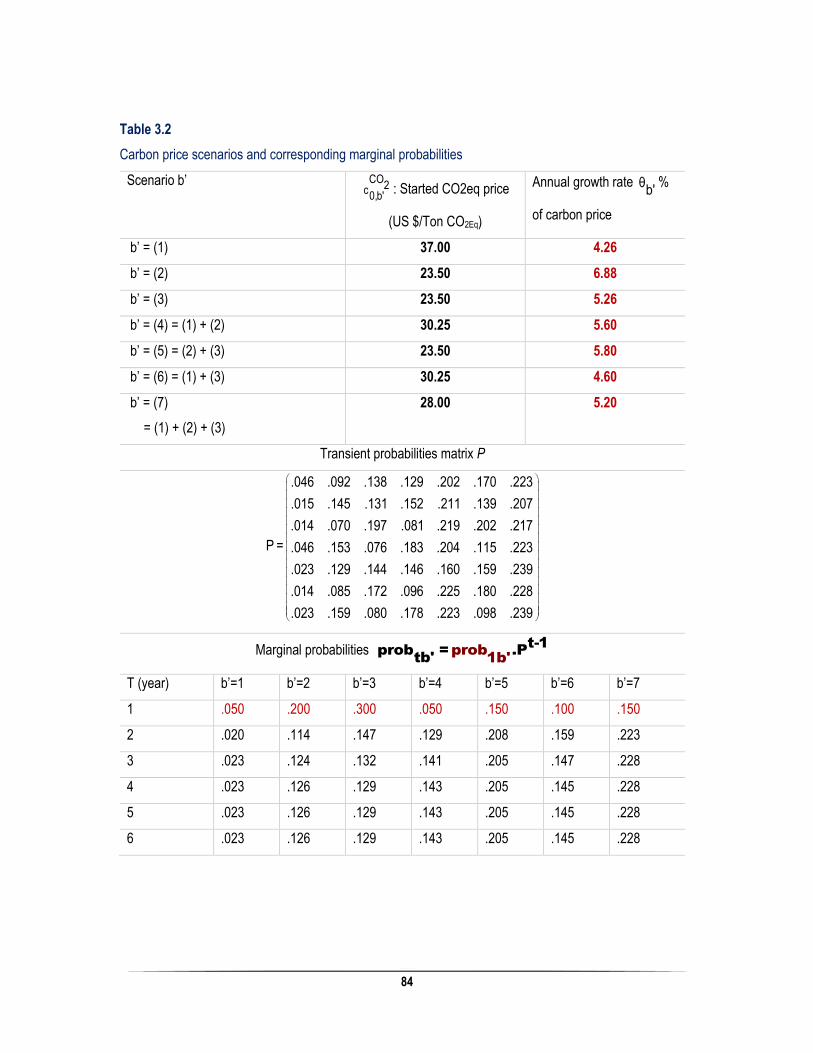
84
Table 3.2
Carbon price scenarios and corresponding marginal probabilities
Scenario b’ CO2c
0,b': Started CO2eq price
(US $/Ton CO2Eq)
Annual growth rate θb'
%
of carbon price
b’ = (1) 37.00 4.26
b’ = (2) 23.50 6.88
b’ = (3) 23.50 5.26
b’ = (4) = (1) + (2) 30.25 5.60
b’ = (5) = (2) + (3) 23.50 5.80
b’ = (6) = (1) + (3) 30.25 4.60
b’ = (7)
= (1) + (2) + (3)
28.00 5.20
Transient probabilities matrix P
.046 .092 .138 .129 .202 .170 .223
.015 .145 .131 .152 .211 .139 .207
.014 .070 .197 .081 .219 .202 .217
P = .046 .153 .076 .183 .204 .115 .223
.023 .129 .144 .146 .160 .159 .239
.014 .085 .172 .096 .225 .180 .228
.023 .159 .080 .178 .223 .098 .239
Marginal probabilities prob1
t-1prob = .P
t b'b'
T (year) b’=1 b’=2 b’=3 b’=4 b’=5 b’=6 b’=7
1 .050 .200 .300 .050 .150 .100 .150
2 .020 .114 .147 .129 .208 .159 .223
3 .023 .124 .132 .141 .205 .147 .228
4 .023 .126 .129 .143 .205 .145 .228
5 .023 .126 .129 .143 .205 .145 .228
6 .023 .126 .129 .143 .205 .145 .228
85
3.3.2. Key data of the second-stage model
Before providing the second-stage programming model, it is worth to prepare some key data required for its
implementation.
The first-stage programming model provide NPareto Solutions. Each solution Sj comprises:
Obj1 (expected total logistics cost); Obj2 (expected total GHG emissions);
Binary decisions of outsourcing transportation, opening warehouses, and opening warehouses as hybrid
distribution centres; and Tactical decisions, which are the quantity of moved products within the closed-loop
SC.
The second-stage model needs essentially two data, to be synthesized from of the result of first stage model
implementation:
- The variation of number of trucks between two consecutive periods t-1, and t, which are assigned to
serve a given destination within the SC network, and
- The optimum expected GHG emissions per period t of this transport configuration.
*** Concerning the number of trucks; the constructive models provided by Ameknassi (2016) lead to
estimate roughly the logistics cost, and corresponding GHG emissions of privately or outsourcing logistics
activities. The fleet size of transportation has been determined as follows, by using the principle of Gencer et
al. (2006); First, clustering around a given destination node within the network; Second, sizing the fleet:
Suppose that a destination Di is served by n origins Oj, and the origins are clustered in two areas which are
separated by sea. The land area 2 comprises k origins plus a port 2, and the land area 1 comprises the
destination Di, (n-k) origins plus a port 1. To move products in the area 2, a configuration of trucks ‘truck2’
with a capacity p
captruck2
, an average of speed v2, and a rate of empty running ε2 is used. While, in the area
1, a configuration of trucks ‘truck1’ with a capacity p
captruck1
, an average speed v1, and a rate of empty
running ε1 is used.

86
Suppose that the FC projects to deliver a fraction β of the demand p
dD
i of product p from the area 2 via
the port 2 & port 1, and the rest 1-β from the area 1. The relation (r*) provides the average number of trucks
required to deliver products p from an origin belonging to area 2 to the port 2, and the average number of
trucks required to deliver products p from the port 2 to the destination Di, both belonging to area 1.
Component 1 : Component 2 :
(r*)
TTrip2
pcap .Teff
β p. .d
Dikp
truck
a
2
rea2
Ttrip1
pcap .Teff
truck
β+(1-β)
pk. d
Dinp
are 1
1
a
All the parameters are defined in the section 2.3.2.1 of chapter 2 (constructive models of computing).
N.B. in the relation (r*, if β = 0 k = 0 , then the size of fleet transportation will be reduced to
Ttrip1pcap .Tefftruck1
1 p. dDinp
For example, in an optimal SC configuration Sj, the number of trucks required to move products from plants
to the warehouse w, at period t is: fleet area2 area1
N = N + Njtw jtw jtw
TTrip2area2
N =pjtw
cap .Teff
tr
β Sjprob . . .q
tbkp,b,m t
u 2
bpmw
ck
&
Ttrip1area1
N =pjtw
c
β
+(1-β)
Sjkprob . . .q
tbnp,b,m ap .T
efftr
tbp
k1
mw
uc
So, the variation of number of trucks between two consecutive periods t-1, and t is:
tΔjw =
t-1 fleet fleet
N -Njtw j(t-1)w
(r*I)

87
***Concerning the GHG emissions per period t of the transport configuration, serving to move products to a
given destination; the first-stage programming model should be asked to edit for each optimal Sj the term
TransportObj2
jtDi, for a given destination Di.
For example, GHG emissions generated by moving products from plants to the warehouse w is by the relation
(r*II) hereunder:
TransportObj2 =
jtw
Sjprob fe xtb Ttbw wb,w
weight δp mw SjSjprob x qtb w.ve tbpmwb,p,m,w Tpmw+
weight δp mwSj
+ prob qtb Sj 3PL.(1-x )e tbpmwb,p,m,w w Tpmw
(r*II)
3.3.3. The Stochastic Combinatory model
For a horizon of multi-periods (indexed t T ), the focal company FC desires selecting the best
decarbonised SC configuration, which minimize a third objective function OBJ3.
OBJ3 is the total expected logistics cost incurred by the FC, after decarbonizing its SC before any LCR
investment; and counteracting uncertain carbon policies by the implementation of a progressive plan of LCR
investment, in freight transportation.
The best decarbonised SC configuration S* corresponds to the Pareto solution Sj, which the minimized
OBJ3Sj is the minimum:
;S*Obj = min minObj3 S Γ = S ,...,S ,...,S
j j NSj 1Pareto
(40)
This best SC design solution S* leads not only to the optimal volume of LCR investment in transportation,
but to the optimal level of 3PL integration within the SC as well.
- Decision variables:

88
The decision variables are binary;
:
l,1y &
tsm
l,2y
tsm
=1, if respectively LCR l1 (l2) approach l is introduced in freight transportation of supply
s to plant m at period t.
=0, otherwise.
l,1y &
tw
l,2y :
tw
=1, if respectively LCR l1 (l2) approach l is introduced in freight transportation of
products to warehouse w at period t.
=0, otherwise.
l,1y &
tv
l,2y :
tv
=1, if respectively LCR l1 (l2) is introduced in freight transportation of products to
warehouse v at period t.
=0, otherwise.
l,1y &
tk
l,2y :
tk
=1, if respectively LCR l1 (l2) is introduced in freight transportation of products to
customer zone k at period t.
=0, otherwise.
:
l,1y &
tiw
l,2y
tiw
=1, if respectively LCR l1 (l2) is introduced in freight transportation of return of products,
from distribution segment i to hybrid warehouse w at period t.
=0, otherwise.
l,1y &
tiu
l,2y :
tiu
=1, if respectively LCR l1 (l2) is introduced in freight transportation of return of products,
from distribution segment i to collection center u at period t.
=0, otherwise.
l,1y &
tm
l,2y :
tm
=1, if respectively LCR l1 (l2) is introduced in freight transportation of recoverable
products to plant m at period t.
=0, otherwise.
l,1y &
tz
l,2y :
tz
=1, if respectively LCR l1 (l2) is introduced in freight transportation of unrecoverable
products to disposal center z at period t.
=0, otherwise.

89
- Parameters:
** Deterministic parameters:
h Average rate of inflation
Costl Cost (in US. $) of individual LCR approach l at the present t=0
υl Time (in years) to pay back the LCR approach l invested
LCRl,1
Average Low Carbon Reduction rate investment l in land area 1 of the SC
LCRl,2
Average Low Carbon Reduction rate investment l in land area 2 of the SC
Factor of linearity for determining the result LCR rate of a group of LCR approaches
ξ Factor defining the budget limitation of FC to invest in LCR approaches of freight
transportation.
** Stochastic parameters:
CO2c0,b'
Started Internal carbon price for scenario b’
θb'
Growth carbon price rate (in fraction), for scenario b’
probtb'
Probability of occurrence of scenario b’, at period t
** Stochastic parameters synthesised from the run of first-stage programming model
TransportObj2 &
jtsm
TransportObj2
j(t-1)sm
Total expected GHG emissions (in tons of CO2eq) to move supply s to plant m, in the
optimal SC configuration Sj, respectively at period t, and period t-1.
TransportObj2 &
jtw
TransportObj2
j(t-1)w
Total expected GHG emissions (in tons of CO2eq) to move products to warehouse w,
in the optimal SC configuration Sj, respectively at period t, and period t-1.
TransportObj2 &
jtv
TransportObj2
j(t-1)v
Total expected GHG emissions (in tons of CO2eq) to move products to warehouse v,
in the optimal SC configuration Sj, respectively at period t, and period t-1.
TransportObj2 &
jtk
TransportObj2
j(t-1)k
Total expected GHG emissions (in tons of CO2eq) to move products to customer zone
k, in the optimal SC configuration Sj, respectively at period t, and period t-1.
TransportObj2 &
jtiw
TransportObj2
j(t-1)iw
Total expected GHG emissions (in tons of CO2eq) to move returned products to hybrid
warehouse w, in the optimal SC configuration Sj, respectively at period t, and period t-
1.

90
TransportObj2 &
jtiu
TransportObj2
j(t-1)iu
Total expected GHG emissions (in tons of CO2eq) to move returned products to
collection center u, in the optimal SC configuration Sj, respectively at period t, and
period t-1.
TransportObj2 &
jtm
TransportObj2
j(t-1)m
Total expected GHG emissions (in tons of CO2eq) to move recoverable products to
plant m, in the optimal SC configuration Sj, respectively at period t, and period t-1.
TransportObj2 &
jtz
TransportObj2
j(t-1)z
Total expected GHG emissions (in tons of CO2eq) to move unrecoverable products to
disposal center z, in the optimal SC configuration Sj, respectively at period t, and period
t-1.
area1N &
jtsm
area2N
jtsm
Number of trucks required in respectively the area 1 (2) for moving supply s to plant m,
at period t, and in Pareto optimal SC configuration Sj.
area1N &
jtw
area2N
jtw
Number of trucks required in respectively the area 1 (2) for moving products to
warehouse w, at period t, and in Pareto optimal SC configuration Sj.
area1N &
jtv
area2N
jtv
Number of trucks required in respectively the area 1 (2) for moving products to
warehouse v, at period t, and in Pareto optimal SC configuration Sj.
area1N &
jtk
area2N
jtk
Number of trucks required in respectively the area 1 (2) for moving products to customer
zone k, at period t, and in Pareto optimal SC configuration Sj.
area1N &
jtiw
area2N
jtiw
Number of trucks required in respectively the area 1 (2) for moving returns from
distribution segment i to hybrid warehouse v, at period t, and in Pareto optimal SC
configuration Sj.
area1N &
jtiu
area2N
jtiu
Number of trucks required in respectively the area 1 (2) for moving returns from
distribution segment i to collection center u, at period t, and in Pareto optimal SC
configuration Sj.
area1N &
jtm
area2N
jtm
Number of trucks required in respectively the area 1 (2) for moving recoverable
products to plant m, at period t, and in Pareto optimal SC configuration Sj.

91
area1N &
jtz
area2N
jtz
Number of trucks required in respectively the area 1 (2) for moving unrecoverable
products to disposal center z, at period t, and in Pareto optimal SC configuration Sj.
tΔjsm
t-1
Variation of number of trucks required to move supply s from corresponding suppliers
to plant m between two consecutive periods t-1 and t, in the optimal SC configuration
Sj
tΔjw
t-1
Variation of number of trucks required to move products from plants to warehouse w
between two consecutive periods t-1 and t, in the optimal SC configuration Sj
tΔjv
t-1
Variation of number of trucks required to move products from plants to warehouse v
between two consecutive periods t-1 and t, in the optimal SC configuration Sj
tΔjk
t-1
Variation of number of trucks required to move products from warehouses to customer
zone k between two consecutive periods t-1 and t, in the optimal SC configuration Sj
tΔjiw
t-1
Variation of number of trucks required to move returns from distribution segment i to
hybrid warehouse w between two consecutive periods t-1 and t, in the optimal SC
configuration Sj
tΔjiu
t-1
Variation of number of trucks required to move returns from distribution segment i to
collection centers u between two consecutive periods t-1 and t, in the optimal SC
configuration Sj
tΔjm
t-1
Variation of number of trucks required to move recoverable products to plant m between
two consecutive periods t-1 and t, in the optimal SC configuration Sj
tΔjz
t-1
Variation of number of trucks required to move unrecoverable products to disposal
center z between two consecutive periods t-1 and t, in the optimal SC configuration Sj
- Objective function:
OBJ3: minimize Obj3Sj
XSj is expressed in the equation (27), and corresponds, for each Pareto solution
S Γ = S ,...,S ,...,Sj j N1
Pareto
, to total cost = A+ B + C - D, where:

92
A: Total logistics cost of the optimal configuration Sj, which is provided by running the first-stage programming
model
B: Total cost of carbon of the decarbonized SC, before any investment in LCR approaches. It is equal to the
average internal carbon price of the multi-period horizon multiplied by Total expected GHG emissions of the
optimal configuration Sj,
C: Total cost of potential investment in LCR approaches, and
D: Savings of the potential LCR investment implemented within different fleet configurations of the SC.
The table 3.3 shows the analytical expression of the objective function OBJ3, to minimize under three types
of constraints:
- Carbon abatement (28) to (36);
- Budget limitation expressed in terms of
total expected logistics costs (37);
- Investment priority (38-45), where the preference
order of investment for the FC is supposed as:
1) Aerodynamics; 2) Low rolling resistance; 3) Driver training; 4) Transmission efficiency; 5) Engine
efficiency, and 6) Hybridization.
- The binary constraints of the decisions variables (46)
Carbon Abatement:
The LCR investment at period t will occurs, if the variation of carbon cost between t-1, and t is greater than
the LRC costs divided by their payback durations, corresponding to probable increase of transportation fleet
between t-1, and t.
We suppose that the individual LCR technologies introduced in MDV & HDV have approximatively the same
cost, but may have different LCR rate (see table 3.1)

93
.
Transportθ .prob .Obj2b' tb' jtsm Cost(t-1)CO l,1 l,2t tl2c .θ (1+h) . .(y +y ).Δjsm ; j, t,s,mb' jtsm jtsm t-1υ0,b' Transport lb' l-prob .Obj2(t-1)b' j(t-1)sm
(28)
.
Transportθ .prob .Obj2b' tb' jtw Cost(t-1)CO l,1 l,2t tl2c .θ . (1+h) . .(y +y ).Δjw ; j, t,wb' jtw jtw t-1υ0,b' Transport lb' l-prob .Obj2(t-1)b' j(t-1)w
(29)
.
Transportθ .prob .Obj2b' tb' jtv Cost(t-1)CO l,1 l,2t tl2c .θ . (1+h) . .(y +y ).Δjv ; j, t,vb' jtv jtv t-1υ0,b' Transport lb' l-prob .Obj2(t-1)b' j(t-1)v
(31)
.
Transportθ .prob .Obj2b' tb' jtk Cost(t-1)CO l,1 l,2t tl2c .θ . (1+h) . .(y +y ).Δjk ; j, t,kjtk jtk t-1υ0,b' b' Transport lb' l-prob .Obj2(t-1)b' j(t-1)k
(32)
.
Transportθ .prob .Obj2b' tb' jtiw Cost(t-1)CO l,1 l,2t tl2c .θ (1+h) . .(y +y ).Δjiw ; j, t, i,wb' jtiw jtiw t-1υ0,b' Transport lb' l-prob .Obj2(t-1)b' j(t-1)iw
(33)
.
Transportθ .prob .Obj2b' tb' jtiu Cost(t-1)CO l,1 l,2t tl2c .θ . (1+h) . .(y +y ).Δjiu ; j, t, i,ujtiu jtiu t-1υ0,b' b' Transport lb' l-prob .Obj2(t-1)b' j(t-1)iu
(34)
.
Transportθ .prob .Obj2b' tb' jtm Cost(t-1)CO l,1 l,2t tl2c .θ . (1+h) . .(y +y ).Δjm ; j, t,mjtm jtm t-1υ0,b' b' Transport lb' l-prob .Obj2(t-1)b' j(t-1)m
(35)
Transportθ .prob .Obj2b' tb' jtz Cost(t-1)CO l,1 l,2t tl2c .θ . . (1+h) . .(y +y ).Δjz ; j, t,zb' jtz jtz0,b' t-1υTransport lb' l-prob .Obj2(t-1)b' j(t-1)z
(36)

94
Binary constraint:
l,1 l,2 l,1 l,2 l,1 l,2 l,1 l,2y ;y ;y ;y ;y ;y ;y ;y ;
jtsm jtsm jtw jtw jtv jtv jtk jtk
l,1 l,2 l,1 l,2 l,1 l,2 l,1 l,2y ;y ;y ;y ;y ;y ;y ;y 0,1
jtiw jtiw jtiu jtiu jtm jtm jtz jtz
j, l, t, s,m,w,v,i,u,z
(46)
Investment Priority constraint:
4,1 5,1 6,1 2,1 1,1 3,1 4,2 5,2 6,2 2,2 1,2 3,2y y y y y y & y y y y y y ;jtsm jtsm jtsm jtsm jtsm jtsm jtsm jtsm jtsm jtsm jtsm jtsm
(38)
&4,1 5,1 6,1 2,1 1,1 3,1 4,2 5,2 6,2 2,2 1,2 3,2y y y y y y y y y y y y ;jtw jtw jtw jtw jtw jtw jtw jtw jtw jtw jtw jtw
(39)
4,1 5,1 6,1 2,1 1,1 3,1 4,2 5,2 6,2 2,2 1,2 3,2y y y y y y & y y y y y y ;jtv jtv jtv jtv jtv jtv jtv jtv jtv jtv jtv jtv
(40)
4,1 5,1 6,1 2,1 1,1 3,1 4,2 5,2 6,2 2,2 1,2 3,2y y y y y y & y y y y y y ;jtk jtk jtk jtk jtk jtk jtk jtk jtk jtk jtk jtk
(41)
4,1 5,1 6,1 2,1 1,1 3,1 4,2 5,2 6,2 2,2 1,2 3,2y y y y y y & y y y y y y ;jtiw jtiw jtiw jtiw jtiw jtiw jtiw jtiw jtiw jtiw jtiw jtiw
(42)
4,1 5,1 6,1 2,1 1,1 3,1 4,2 5,2 6,2 2,2 1,2 3,2y y y y y y & y y y y y y ;jtiu jtiu jtiu jtiu jtiu jtiu jtiu jtiu jtiu jtiu jtiu jtiu
(43)
4,1 5,1 6,1 2,1 1,1 3,1 4,2 5,2 6,2 2,2 1,2 3,2y y y y y y & y y y y y y ;jtm jtm jtm jtm jtm jtm jtm jtm jtm jtm jtm jtm
(44)
.4,1 5,1 6,1 2,1 1,1 3,1 4,2 5,2 6,2 2,2 1,2 3,2y y y y y y & y y y y y yjtz jtz jtz jtz jtz jtz jtz jtz jtz jtz jtz jtz
(45)
j,s,m,w,v,i,u,z

95
Budget limitation:
Depending on its carbon reporting quality to attract investors, and its degree of proactivity to build a
climate resilient SC, the FC defines a factor to express the budget limitation in LCR approaches
investment.
.
Transport TransportObj1 + Obj1
jtsm jtws,m w
Transport Transport+ Obj1 + Obj1
jtv jtkv k
ξ . (1+budget Transport Transport
+ Obj1 + Obj1jtiw jtiu
i,w i,u
Transport Transport+ Obj1 + Obj1
jtm jtzm z
l,1 area1 area1y (N -N )jtsm jtsm j(t-1)sm
Cost .ll,2 area2 area2l,s,m +y .(N -N )jtsm jtsm j(t-1)sm
l,1 area1 area1y (N -N )jtw jtw j(t-1)w
+ Cost .ll,2 area1 area1l,w +y .(N -N )jtw jtw j(t-1)w
y
+ Cost .l
th)
l,1 area1 area1(N -N )jtv jtv j(t-1)v
l,2 area1 area1l,v +y (N -N )jtv jtv j(t-1)v
l,1 area1 area1y (N -N )jtk jtk j(t-1)k
+ Cost .ll,2 area1 area1l,k +y (N -N )jtk jtk j(t-1)k
l,1 area1y (N -Njtiw jtiw
+ Cost .l
area1 )j(t-1)iw
l,2 area1 area1l,i,k +y (N -N )jtiw jtiw j(t-1)iw
l,1 area1 area1y (N -N )jtiu jtiu j(t-1)iu
+ Cost .ll,2 area1 area1l,i,u +y (N -N )jtiu jtiu j(t-1)iu
l,1 area1y (N -Njtm jtm j(t-1)
+ Cost .l
area1 )m
l,2 area1 area1l,m +y (N -N )jtm jtm j(t-1)m
l,1 area1 area1y (N -N )jtz jtz j(t-1)z
+ Cost .ll,2 area1 area1l,z +y (N -N )jtz jtz j(t-1)z
(37)

96
Table 3.3
The objective function of the second-stage stochastic modelling approach
SjObj
1
A
Sj CO t2+ Obj . c .θ .probtb'0,b' b'2 t,b'
B
t l,1 l,2 t t l,1 l,2 t(1+h) .Cost .(y +y ).Δ + (1+h) .Cost .(y +y ).Δl jsm l jw(t-1) (t-1)jtsm jtsm jtw jtwl,t,s,m l,t,w
t l,1 l,2 t t l,1 l,2 t+ (1+h) .Cost .(y +y ).Δ + (1+h) .Cost .(y +y ).Δl jv l jk(t-1) (t-1)jtv jtv jtk jtkl,t,v l,t,k
t+ (1+h) .
l,1 l,2 t t l,1 l,2 tCost .(y +y ).Δ + (1+h) .Cost .(y +y ).Δl jiw l jiu(t-1) (t-1)jtiw jtiw jtiu jtiul,t,i,w l,t,i,u
t l,1 l,2 t t l,1 l,2 t+ (1+h) .Cost .(y +y ).Δ + (1+h) .Cost .(y +y ).Δl jm l jz(t-1) (t-1)jtm jtm jtz jtzl,t,m l,t,z
C
.
l,1 l,2(LCR .y + LCR .y ).Obj2
jtsml,1 l,2jtsm jtsms,m,l
l,1 l,2+ (LCR .y + LCR .y ).Obj2
jtwl,1 l,2jtw jtww,l
l,1 l,2+ (LCR .y + LCR .y ).Obj2
jtvl,1 l,2jtv jtvv,l
l,1 l,2+ (LCR .y + LCR .y ).Obj2
jtkl,1 l,2jtk jtkk,lCO2prob .c .t,b' 0,b'
l,1 l,2
+ (LCR .y + LCR .y ).Obj2jtiwl,1 l,2jtiw jtiwi,w,l
l,1 l,2+ (LCR .y + LCR .y ).Obj2
jtiul,1 l,2jtiu jtiui,u,l
l,1 l,2+ (LCR .y + LCR .y ).Obj2
jtml,1 l,2jtm jtmm,l
l,1 l,2+ (LCR .y + LCR .y ).Obj2
jtzl,1 l,2jtz jtzz,l
t,b'
D
(27)
3.3.4. Discussion
In this section, we discuss some interesting managerial insights, which can be deducted from the
implementation of the two models.
we refer to the working case study of a medium enterprise FC, which manufactures, distributes, and
recover three categories of microwave ovens.
In a horizon of time of 6 years, and in the context of business environment uncertainties, the main
objectives of the Focal Company are:

97
1) responding to 1/6 of the North American market in terms of micro-wave ovens, and exporting a portion
of its production to European market,
2) integrating the logistics outsourcing decision in its SC design, to build a climate resilient SC
3) Optimizing its investment in Low Carbon Reduction of freight transportation to counteract the
uncertain carbon policies
Concerning the implementation of First-stage stochastic modelling: More details are in Ameknassi et
al. (2016).
Concerning the implementation of Second- stage model:
- the code of second-stochastic model, is written in IBM ILOG CPLEX Studio 6.1., and the data of
carbon price stochastic plan, LCR approaches, and the synthesized data (e.g. section 4.2), are
reported in an Excel Microsoft file, and are declared in IBM ILOG CPLEX Studio 6.1.
- By introducing the data of each Sj in the second stage programming model, 9 576 decision
variables must be identified, with the minimized OBJ3j
- The minimum of the minimum OBJ3j corresponds to the best climate resilient SC configuration.
It indicates the optimal integration of 3PL within the SC, and the optimal progressive investment
in LCR freight transportation approaches to counteract the uncertain carbon policies, in the
context of business uncertainty, and within a multi-period horizon of 6 years.
As mentioned in the introduction, Huang et al. (2009) have reported that more than 75% of the Green
House Gases (GHG) emissions of many industry sectors come from their SCs. In Brown (2009), and
according to the World Economic, 15% of GHG emissions come from forward logistics activities, and
about 5% from reverse logistics. The forum suggests thirteen effective strategies to decarbonize the SCs,
and among the most effective ones: Improving the network logistics planning, through 1) global SC
optimization, and 2) LCR approaches investment, notably in the freight transportation technologies.
According to the forum, 24% of carbon reduction may be realized by the first strategy, and according to
Meszler et al. (2015), for tractor with 3 trailers, low Carbon efficiency technology package could result in
LCR of about 48-56%, and cost increase of about 15-25%, with a payback in 1 – 3 years, depending on
the discount rate, and the diesel price. So, 24 % *20 % + (100-24) %*20%*((48+56)/2) % = 12.5%

98
represent the 63.5% of potential carbon reduction that may be realized, by optimizing the global SC, and
investing in LCR freight transport technologies.
However, as the logistics are supposed not to be the core activities of the FC, logistics outsourcing may
be an effective strategy to an optimum level of extent (Das et al. 2006). Regardless the optimality or not
of the common outsourcing transportation level of 70% (Langley & Gemini, 2013), and without considering
carbon cost imposition, the 3PLs may reduce the logistics costs by an average of 15%, but they could
involve a risk of increasing the GHG emissions by 25% (Blanco & Craig, 2009; CDP, 2016). So, the main
objectives are: 1) to optimize the level of logistics outsourcing for balancing the total cost and total GHG
emissions of the climate resilient SC; 2) to determine how this level is dispatched within the echelons of
the SC; 3) to identify how the LCR of freight transportation must be invested inside the different truck
configurations of the SC; and 4) to help future selected 3PLs partners to manage the climate change
risks.
3.4. Conclusion
This work proposes a two-stage stochastic modelling approach to integrate logistics outsourcing
decision in climate change resilient SC design problems. As part of Paris negotiations, 187 countries
submitted Post-2020 Intended Nationally Determined Contributions (INDCs) to the United Nations
Framework Convention of Climate Change (UNFCCC). These climate commitments mean more legal
requirements of businesses, and more climate actions are needed to support the climate change
resilience of focal companies (FCs) and their suppliers within the SCs. According to the last report of
Carbon Disclosure Project CDP report, the awareness and actions of suppliers vis-à-vis the climate risks
remain insufficient to build resilient SCs, and FCs should help their suppliers to manage effectively their
climate risks. We consider the 3PLs as potential important partners of a FC to effectively circulate the
sustainable practices within its global SC, and the integration of logistics outsourcing decisions in the
design of sustainable SC problem is of strategic importance. The first stage of stochastic modelling
approach has been presented in our recent work submitted to the International Journal of Production
Economics, and consists of suggesting a Stochastic, Multi-Objective, Multi-Period, and Multi-Product
programming model, integrating logistics outsourcing decisions in a closed-loop SC design, before any

99
investment in emerging Low Carbon Reduction (LCR) Technologies. The result has been a set of Pareto
optimal SC configurations, which identify the logistics activities to be outsourced from those to be
performed in-house. A multi-criteria analysis would be suggested to select the best SC configuration,
however, we suggest a second-stage stochastic model, as a normative decision, not only to select the
best SC configuration, but to determine the optimal progressive LCR investment in freight transportation,
for counteracting the uncertain future carbon policies, as well. To do so, we; 1) Synthesized the evolution
of heterogeneous transportation fleet size of each Pareto solution of the 1st stage model; 2) Established
a Carbon stochastic price plan in the context of voluntary disclosure Carbon regime; 3) Proposed a
Stochastic, Mono-Objective, and Multi-Period Combinatory programming model, to minimize the total
logistics cost, after incurring carbon cost, and investing in Low Carbon Reduction of freight transportation.
The model is subject to carbon abatement constraint, and Low Carbon reduction approaches’
prioritization. Running the 2d stage Combinatory model leads to identify optimal levels of 3PL integration,
and Low Carbon investment.
This work presents some limitations, that it is worth to deal with in further researches. The second-stage
stochastic model consider only the LCR technologies in freight transportation, but should be extended to
other energy efficiencies related to bio-fuel utilization, and related to warehousing & material handling.
The stochastic plan of carbon price establishment, in the context of voluntary carbon disclosure regime,
remain open to a lot of improvements, because the volatile nature of carbon prices. The operational
management of empty back hauls may lead to develop more effective transportation itineraries, and more
effective transportation schedules. So, the evolution of fleet size may be subject to serious modifications,
which affect the optimality of the second-stage model. Finally, the second-stage stochastic modelling
approach should be completed by a supplier robust selection approach to build sustainable SCs.

100
References
Allaoui H. & Goncalves G., 2013. Green Supply Chain: Challenges and opportunities. Supply Chain
Forum: An International Journal, 14 (2), 1–3
Andrew B., 2008. Market failure, government failure and externalities in climate change mitigation: the
case for a carbon tax. Public Adm. Develop. 28 (5), 393-401.
Ameknassi L., Ait-Kadi D., Rezg N., 2016. Integration of Logistics Outsourcing Decisions in a Green
Supply Chain Design: A Stochastic Multi-Objective Multi-Period Multi-Product Programming Model.
International Journal of Production Economics, 182 (c), 165-184.
Aravendan M., Panneerselvam, R. 2015. Development and Comparison of Hybrid Genetic Algorithms for
Network Design Problem in Closed Loop Supply Chain. Intelligent Information Management, 7, 313-
338. http://dx.doi.org/10.4236/iim.2015.76025
Blanco E. E., & Craig A. J., 2009. The Value of Detailed Logistics Information in Carbon Footprint. MIT
Center for Transport & Logistic; Cambridge MA, USA; http://6ctl.mit.edu/research
Brown D., 2010. Technologies and Approaches to Reducing the Fuel Consumption of Medium- and
Heavy-Duty Vehicles. Committee to assess Fuel Economy Technologies for Medium-and-Heavy Duty
Vehicles; 250 pages. Copyright © National Academy of Sciences. All rights reserved.
available at http://www.nap.edu/catalog.php?record_id=12845
Browne P., Gawel A., Andrea Brown A., Moavenzadeh J., & Krantz R., 2009. Supply Chain De-
carbonization: The role of Logistics and Transport in reducing Supply Chain Carbon Emissions, p. 1–
41. World Economic Forum. Geneva.
http://www3.weforum.org/docs/WEF_LT_SupplyChainDecarbonization_Report_2009.pdf
CDP & BSR, 2016. From Agreement to Actions: Mobilizing Suppliers towards a Climate Resilient World.
Carbon Disclosure Project Supply Chain Report 2015-2016; pp. 1-36. Available at www.cdp.net
CDP, 2015. Putting a price on risk: Carbon pricing in the corporate world. Carbon Disclosure Project
Report 2015 v.1.3; pp.1-.68.
Chiu Y., Lin P-C., & Hsu H-H., 2011. Considering 3PL in reverse logistics. Journal of Chinese Institute of
Industrial Engineers, 28(7): 512-520.
Das A., Narasimhan R., & Talluri S., 2006. Supplier integration- Finding an optimal configuration. Journal
of Operation Management, 24 (5), 563–582.
Demirel O.N., Gökçen H., 2008. A mixed-integer programming model for remanufacturing in reverse
logistics environment, Int. J. Adv. Manuf. Technol. 39 (11–12), 1197–1206.
El-Sayed M., Afia N., El-Kharbotly A., 2010. A stochastic model for forward–reverse logistics network
design under risk, Comput. Indus. Eng. 58. 423–431.
Etchart A., Sertyesilisik B., Mill G., 2012. Environmental effects of shipping imports from China and their
economic valuation: the case of metallic valve components. J. Clean. Prod. 21 (1), 51-61.

101
Evangelistia, P., Huge-Brodin, M., Isaksson, K., Sweeney, E., 2011.The Impact of 3PL’s Green Initiatives
on the Purchasing of Transport and Logistics Services: An Exploratory Study, p: 1–15. Proceedings of
the 20th International Purchasing and Supply Education and Research Association (IPSERA)
Conference, Maastricht University.
Available at: http://arrow.dit.ie/nitlcon
Facanha C., & Horvath A., 2005. Environment Assessment of Logistics Outsourcing. Journal of
Management in Engineering, 21 (1), 27–37.
Fareeduddin M., Adnan H., Syed M. N., Selim S. Z., 2015. The Impact of Carbon Policies on Closed-loop
Supply Chain Network Design. Procedia CIRP 26, 335–340.
Gao N., & Ryan S. M., 2014. Robust design of a closed-loop supply chain network for uncertain carbon
regulations and random product flows. EURO Journal on Transportation and Logistics. 3 (1), 5–34.
Gencer C, Top I, Aydogan E. K.2006. A new intuitional algorithm for solving heterogeneous fixed fleet
routing problems: passenger pickup algorithm. Applied Mathematics and Computation; 181(2), 1552–
1567.
Grant D., Bergstrand K., Running K., 2014. Effectiveness of US State policies in reducing CO2 emissions
from power plants. Nature Climate Change, 4, 977-982. DOI: 10.1038/NClimate2385.
Hoen K. M. R., Tan T., Fransoo J.C., vanHoutum G. J., 2014. Effect of carbon emission regulations on
transport mode selection under stochastic demand. Flexible Services Manufacturing Journal. 26 (1–2),
170–195.
Horn H. S., 1975. Markovian Properties of Forest Succession- In: Cody M. L., and Diamond J. M. (ed.).
Ecology and Evolution of Communities. Harvard University Press; Cambridge Mass, pp 196-211.
Huang Y. A., Weber C. L., & Mathews H. S., 2009. Categorization of Scope 3 Emissions for Streamlined
Enterprise Carbon Foot printing. Environment Science and Technology, 43 (22), 8509–8515.
Jaber M. Y. & Goyal S. K., 2008. Coordinating a Three-level Supply Chain with Multiple Suppliers, a
Vendor, and Multiple Buyers. International Journal of Production Economics, 116, 95-103.
Jayaram J. & Tan K-C., 2010. Supply chain integration with third-party logistics providers. International
Journal of Production Economics, 125 (2), 261–271.
Knox-Hayes J., & Levy D., 2011. The politics of carbon disclosure as climate governance. Strategic
Organization, 9 (1), 1-9. Doi: 10.1177/1476127010395066
Kossoy A., Peszko G., Oppermann K., Prytz N., Klein N., Blok K., Lam L., Wong L., Borkent B. 2015.
State and Trends of Carbon Pricing 2015 (September), by World Bank, Washington, DC. Doi: 10.1596/
978-1-4648-0725-1
Kraljic, P. 1983. Purchasing must become Supply Management, Harvard Business Review, 61 (5), 109-
114.
Langley J. Jr. & Cap Gemini, 2013. The State of Logistics Outsourcing: Results and Findings of the 17th
Annual Study. Third-Party Logistics Study, Cap Gemini consulting, 1–40. Available at:
http://www.capgemini-consulting.com

102
Lee H.L., 2002. Aligning Supply Chain Strategies with product uncertainties. California Management
Review. 44 (3), 105–119.
Lutsey N., Langer T., & Khan S., 2014. Stakeholder workshop report on tractor-trailer efficiency
technology in the 2015-2030 timeframe. International Council on Clean Transportation, American
Council for an Energy-Efficient Economy, University of California. Washington, D.C.
Lomborg B., 2016. Impact of Current Climate Proposals. Global Policy. 7 (1), 109-118. doi: 10.1111/1758-
5899.12295 Published by Durham University & John Wiley & Sons Ltd.
Matisoff D. C., Noonan D. S., O’Brien J. J., 2013. Convergence in Environmental Reporting: Assessing
the Carbon Disclosure Project. Business Strategy and the Environment. 22, 285-305. Doi:
10.1002/bse.1741.
McKinnon A. & Piecyk M., 2011. Measuring and Managing CO2 Emissions of European Chemical
Transport. Cefic - The European Chemical Industry Council, http://www.cefic.org
Meszler D., Lutsey N., Delgado O., 2015. Cost Effectiveness of Advanced Efficiency Technologies for
Long-Haul Tractor-Trailer in The 2020-2030 Time Frame; International Council on Clean Transportation;
p.1-63;
http://www.theicct.org/sites/default/files/publications/ICCT_tractor-trailer_tech-cost
effect_20150420.pdf
Meyn S. P., & Tweedie R. L., 1996. Markov Chains and Stochastic Stability. Springer-Verlag London
Limited. Doi 10.1007/ 978-1-4171-3267-7. ISBN 978-1-4471-3267-7 (eBook).
Min H., Ko H.J., 2008. The dynamic design of a reverse logistics network from the perspective of third-
party logistics service providers, Int. J. Product. Econ. 113. 176–192.
Mirzapour Al-e-hashem S.M.J., Baboli A., Sazvar Z., 2013. A stochastic aggregate production planning
model in a green supply chain: Considering flexible lead times, nonlinear purchase and shortage cost
functions. European Journal of Operational Research 230 (1), 26–41
Montoya-Torres J.R., Gutierrez-Franco E., & Blanco E.E. 2015. Conceptual framework for measuring
carbon footprint in supply chains. Production Planning & Control: The Management of Operations. 26
(4), 265–279.
Mukhopadhyay S. K. & Setaputra R., 2006. The Role of 4PL as the Reverse Logistics Integrator: Optimal
Pricing & Return Policies. International Journal of Physical Distribution & Logistics Management; 8 (9);
716-729.
National Research Council (NRC) Committee, 2010. Technologies and Approaches to Reducing the Fuel
Consumption of Medium- and Heavy-Duty Vehicles. National Research Council & Transportation
Research Board. 1-250. The National Academies Press. Available at:
http://www.nap.edu/catalog.php?record_id=12845
Nordhaus W. D., 2007. A review of the “Stern review on the economics of climate change”. J. Econ. Lit.
45 (3), 686-702.

103
Nouira I, Hammami R., Frein Y., Temponi C. 2016. Design of forward supply chains: Impact of a carbon
emissions-sensitive demand. International Journal of Production Economics. 173, 80–98.
Ordoobadi S., 2005. Development of a Decision Model for Strategic Outsourcing. Journal of Applied
Business and Economics, 5 (2), 7-24.
Ordoobadi S. 2010. Application of AHP and Taguchi loss functions in supply chain. Industrial
Management & Data Systems. 110 (8), 1251-1269.
Pishvaee M.R., Kianfar K., Karimi B., 2010. Reverse logistics network design using simulated annealing,
Int. J. Adv. Manuf. Technol. 47, 269–281.
Pishvaee M.S., Fariborz Jolai F., & Razmi J., 2009. A stochastic optimization model for integrated forward/
reverse logistics network design. Journal of Manufacturing Systems, 28 (4), 107–114.
Pishvaee M.S., Fathi M., & Jolai F., 2008. A fuzzy Clustering-based method for scenario analysis in
strategic planning: The case of an Asian pharmaceutical company. South African Journal of Business
Management, 39 (3), 15–25
Prahalad C. K. & Hamel G., 1990. The Core Competence of the Corporation. Harvard Business Review,
79-91.
Quinn J. B. & Hilmer G. F., 1994. Strategic Outsourcing. Sloan Management Review, 43-55.
Ramezani M., Bashiti M., & T-Moghaddam R., 2013. A new multi-objective stochastic model for a
forward/reverse logistic network design with responsiveness and quality level. Applied Mathematical
Modeling, 37 (1-2), 328–344.
Rosenzweig E.D., Roth A.V., Dean Jr. J.W., 2003. The influence of an integration strategy on competitive
capabilities and business performance: an exploratory study of consumer products manufacturers.
Journal of Operations Management 21 (4), 437-456
Ross S. M., 2009. Introduction to Probability Models. Tenth Edition. Elsevier Academic Press. ISBN: 978-
0-12-375686-2.
Rydge, J., 2015. Implementing Effective Carbon Pricing. Contributing paper for seizing the Global
Opportunity: Partnerships for Better Growth and a Better Climate. New Climate Economy, London and
Washington, DC. Available at: http://newclimateeconomy.report/misc/working-papers/.
Salema M. I., Po’voa A.P.B., Novais A.Q., 2006. A warehouse-based design model for reverse logistics,
J. Oper. Res. Soc. 57 (6), 615–629.
Savaskan R. C., Bhattacharya S. & Van Wassenhove L. N., 2004. Closed-loop supply chain models with
product remanufacturing. Management Science. 50 (2), 239-252.
Sazvar Z., Mirzapour Al-e-hashem S.M.J., Baboli A., Akbari Jokar M.R., 2014. A bi-objective stochastic
programming model for a centralized green supply chain with deteriorating products, International
Journal of Production Economics, 150: 140–154
Sharpe B. & Muncrief R., 2015. Literature review: Real-World Fuel Consumption of Heavy-Duty-Vehicles
in the United States, China, and the European Union. International Council on Clean Transportation, 1-
27.
104
http://www.theicct.org/sites/default/files/publications/ICCT_HDV_FC_lit-review_20150209.pdf
Tseng S., & Hung S., 2014. A strategic decision-making model considering the social costs of carbon
dioxide emissions for sustainable supply chain management. Journal of Environmental Management,
133, 315–322.
Vonderembse M. A., Uppal M., Huang S. H., & Dismukes J. P. 2006. Designing Supply Chains: Towards
theory development. Int. Journal of Production Economics, 100 (2), 223–238.
Wang F., Xiaofan Lai X., & Shi N., 2011. A Multi objective Optimization for Green Supply Chain Network
Design. Decision Support Systems; Volume 51 (2), 262–269.
Webster S. & Mitra S., 2007. Competitive strategy in remanufacturing and the impact of take-back laws.
Journal of Operations Management; 15 (3), 1123–1140.
Wolf, C., & Seuring, S., 2010. Environmental impacts as buying criteria for third party logistical services.
International Journal of Physical Distribution & Logistics Management. 40 (1): 84-102.
WRI & WBCSD, 2013. Required Greenhouse Gases in Inventories; World Resources Institute and World
Business Council for Sustainable Development, p: 1–9.
http://www.ghgprotocol.org/files/ghgp/NF3Amendment_052213.pdf.

105
Chapter 4:
Third Party Logistics Providers Selection in the Context of
Sustainable Supply Chains:
A Robust Integrated Approach
Highlights:
The logistics activities being outsourced are modelled as a sustainable business process;
Criteria, risks, and two quality engineering functions are defined to optimize the process;
QFD-Fuzzy AHP is used to parametrize the factors influencing the 3PL selection;
Taguchi Robust Design is used to optimize the settings of selection criteria;
DEA is used to shorten the list of candidates, to be compared to the optimum of Taguchi.

106
Résumé
Ce chapitre développe une approche intégrée robuste pour sélectionner un prestataire logistique « Third-
Party Logistics (3PL) », dans le cadre des chaînes logistiques durables. Elle ne considère que les activités
logistiques à externaliser comme un processus d’affaires qui transforme les inputs « critères de
Ressources et Capabilités » en outputs « critères de Capacités & Performances », pendant qu’il est
soumis à des perturbations « Risques d’Affaires ». Deux fonctions de transfert ont été considérées pour
représenter la valeur ajoutée du processus : Efficacité et Robustesse. Tout d'abord, l’Analyse
d’Enveloppement des Données (DEA) est effectuée pour limiter la liste des candidats 3PL, seulement à
ceux d’efficience relative comparable. Deuxièmement, l’outil intégré QFD-Fuzzy AHP est effectuée pour
paramétrer les facteurs influant sur le processus de sélection des 3PLs. Troisièmement, La technique de
Conception Robuste est effectuée pour trouver l’optimum de Taguchi; un 3PL "virtuel", dont les critères
de sélection sont optimisés. Enfin, les candidats 3PL seront comparés à l'optimum, et le lauréat doit être
le plus proche de cet optimum. Ainsi, les coûts supplémentaires des ressources et des capacités pas
nécessairement utilisées seraient évités, et le processus externalisé serait quasiment le plus efficient et
le plus résilient aux perturbations. Un exemple illustratif de la sélection d’un 3PL pour la logistique inverse
est fourni pour démontrer l'applicabilité de l'approche proposée, et pour mettre en évidence les faiblesses
des approches de sélection les plus populaires.

107
Abstract
This chapter develops a robust integrated approach to select a Third-Party Logistics provider (3PL), in
the context of sustainable Supply Chains (Scs). It considers logistics activities being outsourced as a
business process transforming inputs “resources & capabilities” into outputs “Capacity & performances”,
while is being submitted to disruptions “Business risks”. Two transfer functions: Efficiency & Robustness,
are considered to represent the value added of the process. First, DEA method is performed to shorten
the list of 3PL candidates, to only those of comparative relative efficiencies. Second, multi-stage QFD-
Fuzzy AHP is performed to parametrize the factors influencing the process of 3PL selection. Third, Robust
Design Technique is performed to find the Taguchi optimum; a “virtual” 3PL, in which the settings of
selection factors are optimized. Finally, the 3PL candidates will be compared to the optimum, and the
winner should be the closest one to this optimum. Doing so, the incremental costs of idle resources and
capabilities will be avoided, and the process being outsourced is nearly the most efficient and the most
resilient. An illustrative example of 3PL selection for reverse logistics is provided to demonstrate the
applicability of the suggested approach, and to show the weaknesses of the most popular selection
approaches.
Keywords:
- Sustainable Supply Chains;
- Third Party logistics providers;
- Data Envelopment Analysis;
- Fuzzy AHP/Quality Function Deployment;
- Taguchi Robust Design.

108
4.1. Introduction
In “Sustainable” SCs, environmental and social criteria need to be fulfilled by the members to remain
within the SCs, while it is expected that competitiveness would be maintained through meeting customer
needs, and related economic criteria (Seuring & Müller, 2008). Nowadays, more than 8 000 businesses
around the world have signed the United Nation Global Compact pledging to show good global citizenship
in the areas of human rights, labor standards and environmental protection (Wharton, 2012). Media &
Non-Governmental Organizations (ONG) continue to put more pressure on public & private organizations
to control their outsourcing practices, while considering all the aspects of sustainability in their call for
tenders (Sullivan & Ngwenyama, 2005).
Outsourcing is a flexible strategy, which involves allocating or reallocating business activities from an
internal source to an external source (Schniederjans et al. 2015). It is currently one of the hottest topics
in business practices; in particular in the field of logistics. Currently, about 40% of the global logistics
activities (e.g. Inbound, outbound, and reverse logistics) are outsourced to 3PLs (Langley & Capgemini,
2015). According to the recent study of Langley & Capgemini (2013), Total of logistics expenditure
represents 12 to15% of the sale revenue of industrial organizations, and logistics outsourcing can reduce
the logistics cost by 15%, the inventory cost by 8%, and the logistics fixed-asset by 26%. Logistics service
provider (3PL) as a supplier of services, has a potential role to act as a mediator between interfaces of a
Sustainable SC. It may help a company to facilitate the implementation of sustainable practices in both
upstream and downstream of the SC (Lieb & Lieb, 2010). However, according to Evangelista et al. (2011);
Wolf & Seuring (2010), and Blanco & Craig (2009), 3PL seem not undertake concrete sustainable
initiatives vis-à-vis the energy efficiency, the Green House Gas emissions, the traffic congestion, and the
working conditions. Their role seems rather to be concentrated on the deployment of conventional
competitiveness criteria such as cost, quality, and flexibility. Whence the risk involved by the logistics
outsourcing strategy to miss the sustainable development commitments. In Langley & Capgemini (2014),
every year about 30% of 3PL’ users decide systematically to return to in-source some or all of their
logistics needs, despite would this can result in terms of loss of time, effort and money.

109
In supply chain design, and logistics literature, logistics outsourcing decisions have been investigated
by asking the key questions; Why? What? Where? Who? How? & To what extent? (Hätönen & Eriksson,
2009). The reader may consult these papers, for more details around the subject:
- “Why?” outsourcing logistics (Anderson et al. 2011; Hsiao et al. 2010; Jayaram & Tan, 2010);
- “What?” logistics activities should be outsourced (Serrato et al. 2007; Savaskan et al. 2004);
- “Where?” outsourcing logistics (Bunyaratavej et al. 2007; Graf & Mudambi, 2005);
- “Who?” is the most effective 3PL to select for performing a logistics activity (Ho et al. 2012;
Hamdan & Rogers, 2008);
- “How?” to manage the relationship between outsourcing companies and 3PLs (Yang & Zhao,
2016; Flynn et al. 2010); and
- “To what extent?” 3PL may be integrated to optimize the green SC configuration (Ameknassi et
al. 2016)
In this work, we suppose that the Focal Company FC has designed its green SC, and determined the
optimal configuration of the SC which strategically, and financially distinguishes the logistics activities to
outsource, from those to perform in house (Ameknassi et al. 2016). We focus on the question of “Who?”
is the most efficient 3PL to select in the context of a sustainable SC.
Developing a sound 3PL selection decision making, in the context of sustainable SCs depends on the
ability to identify and parametrize the most relevant factors, that influence the sustainability of the logistics
process being outsourced. It depends also on the ability to evaluate the process efficiency, which is
subjected to inherent disturbances affecting the process within the SC. We shall investigate in this paper
the 3PL selection criteria, and the popular selection methods used to deal with the supplier selection
problem, and identify the impediments applying them in the context of sustainable SCs. Then we suggest
a Robust Integrated Approach: The ‘‘DEA-QDF/fuzzy Analytic Hierarchic Process AHP-Taguchi Robust
Design’’. This approach is intended to be:
- Relevant, by appropriately identifying, categorizing, and calibrating the sustainable selection
criteria;
- Consistent, by ensuring the coherence of criteria with the real logistics needs, and the business
strategies of the outsourcing company; and

110
- Robust by capturing the uncertainties related to the uncontrollable risk factors influencing the
efficiency of the logistics process being outsourced.
An example of 3PL selection problem for reverse logistics is introduced to construct the integrated
approach, by showing the pros and the cons of the most popular selection methods.
To the knowledge of the authors, it is the first time the orthogonal Taguchi Robust Design plan is
transferred from engineering process robust optimization to 3PL selection problem, to consider the
resource limitations and capture the business uncertainties, which are generally neglected by the previous
researches in the field.
The remainder of this chapter is organized as follows. After a brief overview of the 3PL selection problem
in the section 4.2, we define in the section 4.3 the methodology to deal with the selection of 3PL in the
context of Sustainable SCs. From the literature, we suggest the sets of business strategies, and generic
logistics requirements of different logistics processes within a sustainable SC. We suggest, categorize,
and calibrate the main factors influencing the efficiency and the robustness of the logistics process being
outsourced. Then, we present in three phase the procedure for selecting a sustainable 3PL. In the section
4.4, we demonstrate the applicability of the robust integrated approach by performing an illustrative
example of 3PL selection problem for reverse logistics. We provide the analytical models of DEA, QFD-
based methods, and Taguchi robust design technique, and show progressively their pros and cons, and
we discuss some interesting managerial insights concerning the 3PL selection problem. Finally, in the
section 4.5 we draw the conclusion.
4.2. Problem of 3PL Selection
Third-Party logistics (3PL), is a company that works with shippers on a contract basis, to manage their
logistics operations. According to Bask (2001), it may offer three distinguished services:
- Routine services which include all types of basic transportation and warehousing;
- Standard services which contain some easy customized operations like special transportation
where products need to be cooled, heated or moved in tanker trucks; and
- Customized services which consist of different postponement services like light assembly of
product, packing product and/or recovery, and reverse logistics operations.

111
Sink & Langley (1997) had provided a conceptual model of the 3PL outsourcing process with five stages:
1) Identify the need to outsource logistics; 2) develop feasible alternatives; 3) evaluate and select the 3PL
supplier; 4) implement service; and 5) ongoing service assessment. The 3PL selection is a multi-criteria
problem, in which most of the selection criteria are conflictual. Recent works of 3PL selection have
suggested many selection criteria, and have adopted a variety of evaluation methods, that may be
summarized in the following subsections:
4.2.1 Selection Criteria
In the logistics literature, the number of proposed selection criteria for a decision making varied between
4 and 31, with an average number of 9 criteria (Wittstruck & Teuteberg, 2011), and the logistics activities
being outsourced might be the general logistics or the reverse logistics;
Two examples of general logistics outsourcing are: Jayaram & Tan, (2010) suggested 6 criteria: 1)
Scope of resources; 2) Industry knowledge; 3) Commitment to quality; 4) Ability to meet delivery due
dates; 5) Financial stability and staying power; and 6) Ability to respond to unexpected demand. In a
recent empirical study, Coltman et al. (2011) proposed 10 criteria: 1) Reliable performance; 2) Delivery
speed; 3) Professionalism; 4) Service handling and support, 5) Supply chain flexibility; 6) Track and trace;
7) Service recovery; 8) Supply chain capacity; 9) Proactive innovation, and 10) Parity price.
Two other examples of reverse logistics outsourcing are: Meade & Sarkis (2002) had suggested 4
criteria: 1) Location of product in its lifecycle; 2) Organization’s strategic performance criteria; 3) Reverse
logistics processes functions required by the organization; and 4) Organization role of reverse logistics.
While Efendigil et al. (2008) have proposed 12 criteria: 1) On-time delivery; 2) Fill rate; 3) Service quality;
4) Unit operation cost; 5) Capacity usage; 6) Total order cycle time; 7) System flexibility index; 8)
Integration level; 9) Increment in market share; 10) Research & Development; 11) Environmental
expenditure; and 12) Customer satisfaction.
In the context of sustainable SCs, except very few researches such as (Presley et al. 2007; Bai & Sarkis,
2010; Wittstruck & Teuteberg, 2011), substantial researches on 3PL selection did not explicitly considered
the social and environmental criteria, in their decisional structure. Even in the area of material supplier
selection, only the traditional criteria (price, quality, innovation, flexibility, financial stability…) and the

112
green criteria (i.e. green design, pollution prevention, green image, green capability, and environmental
management) were focused on (Akman (2015; Awasthi et al. 2011). Wittstruck & Teuteberg (2011)
provided a holistic approach to select a recycling partner for German electrics and electronics industry.
They suggested 9 sustainable criteria, namely: 1) Price; 2) Financial Capability; 3) Recycling Capability;
4) Quality of Recycling Processes; 5) Effective Implementation of Environmental Management Systems;
6) Standardized Health and Safety Conditions; 7) Sustainable Image; 8) Efficient Information Technology-
Interfaces; and 9) Know-How in the field. While Presley et al. (2007) have proposed a decisional structure,
in which 3 economic metrics (Net Present Value; Delivery performance; Supply chain cycle time), 3
environmental metrics (Waste generated, Improved compliance, % Product reclaimed), and 3 social
metrics (Internal human resource, External population, and Stakeholders participation) represent the
selection criteria of the reverse logistics outsourcing. Finally, Hosseini & Baker (2016) stress the
importance of integrating the resilience concept in supplier selection problem. Resilience as defined by
Sheffi (2005), which is the inherent ability of a system or organization to withstand the effect of a disruption
(e.g. demand & supply risks, natural disasters, man made events, and business vulnerability), to maintain
or recover its steady state behavior, thereby allowing it to continue normal operations after a disruptive
event. So, Hosseini & Baker (2016) recommend to complete the decision structure of material supplier
selection problem by the resilient criteria.
The present paper looks for enriching the logistics literature in the sense of identifying, categorizing,
and determining the magnitudes of the main parameters impacting the 3PL selection, in the context of
sustainable SCs. The Economic, social, and environmental criteria should be considered in the decision
structure to select the most efficient candidate. The risk factors related to: Demand; Supply; Environment;
Social Acceptability; and Outsourcing process himself affect seriously the efficiency and the stability
(robustness) of the logistics process being outsourced, and should be considered in the decision
structure. We consider the risk factors as extra resources and capabilities to maintain the efficiency of the
logistics process, depending on the relative importance of each one. Doing so, an by mean of an
appropriate evaluation method, the consistency and the robustness of the 3PL selection process will be
achieved.

113
4.2.2. Evaluation Methods
In Aguezzoul (2014), the methods for evaluation and selection supplier can be classified into seven
categories:
1) Linear weighting models: AHP / TOPSIS / ANP (Jayant et al. 2014; Dargi et al. 2014);
2) Mathematical programming models: Multi-objective programming / Goal programming / Data
Envelopment Analysis DEA (Zhang et al. 2013; Karimi & Rezaeian, 2014; Mahdiloo et al. 2015);
3) Outranking Methods like ELECTRE (Vahdani et al. 2010) and PROMETHEE (Chen et al. 2011);
4) Artificial intelligence: Case Based Reasoning / Artificial Neural Network (Yan et al. 2003);
5) Methods Based on Costs: Activity Based Costing / Total Cost of Ownership (Bhutta & Huq, 2002);
6) Statistical approaches: Mean & Correlation matrix / Payoff matrix, Vendor profile analysis / Logistics
Regression Model (McGinnis et al. 1995); and
7) Integrated approaches such as QFD-DEA (Karsak & Dursun, 2014); AHP-PROMETHEE (Bansal &
Kumar, 2013); QFD-Fuzzy AHP (Ho et al. 2012).
According to Ho et al. (2010), the individual DEA method and the AHP-based methods seem to be the
most prevalent ones;
Data Envelopment Analysis DEA is commonly used to compare the efficiency of a number of Decision
Making Units DMUs (e.g. the 3PL candidates). It is a linear programming procedure for a frontier analysis
of inputs and outputs (Charnes et al. 1978). Inputs represent the deployed resources and capability of the
DMU, and the outputs represent the its performances, and the efficiency is the ratio of outputs to the
inputs, the selected 3PL is the most efficient among the DMUs. (See analytical details in the next section,
and the illustrative example). DEA has attracted more attention mainly because of: 1) can handle multiple
tangible and intangible inputs and outputs; 2) its robustness, and can handle deterministic or stochastic
inputs and outputs; and 3) doesn't require an assumption of a functional form of the efficiency (Ho et al.
2010). However, DEA presents some drawbacks: 1) The practitioners may be confused with input and
output criteria. 2) the subjective assignment of ratings to intangible criteria may affect the value of the
efficiency. 2) DEA is good at estimating "relative" efficiency of a DMU, but it converges very slowly to
"absolute" efficiency. In other terms, DEA does not compare to a theoretical maximum; and 3) DEA is a

114
nonparametric technique, and it cannot handle the relative importance attributed to each output or input,
within the decision structure.
The wide applicability of AHP based methods is due their simplicity, ease of use, and great flexibility.
The AHP hierarchy consists of evaluating the selection criteria, then evaluating the potential candidate
relatively to those criteria. The candidates are ranked, and the most effective one is selected (Saaty,
1980). The integration of Quality Function Deployment QFD to AHP (Rajesh et al. 2011) allows to
construct a coherent, and consistent relationship between the business strategies of the company and
the selection criteria, by affecting the rights weights to the criteria. One of the issues in relation to the AHP
method is the subjective judgments in pairwise comparison matrices. Fuzzy logic theory (Zadeh, 1965),
and DEA method have been suggested to remedy to this inconvenience. Ho et al. (2012) proposed QFD-
Fuzzy AHP, in which fuzzy triangular number have been utilized to capture the vagueness of judgments
involved by a group of decision makers, when establishing pairwise matrix between business strategies
and requirements, between requirements and criteria, and between criteria and supplier candidates.
Authors such as Kuo & Lin (2012) have suggested ANP rather than AHP to capture the interdependency
between the criteria, and introduced the DEA method to provide pairwise matrices without any reference
to individuals’ opinions.
In the context of sustainable SC, the question that has to be asked is: Do we seek for selecting the
most effective 3PL candidate, or the most efficient one?
According to ISO definitions, in Frøkjær et al. (2000), Effectiveness is the accuracy and completeness
with which users achieve certain goals. Efficiency is the relation between (1) the accuracy and
completeness with which users achieve certain goals, and (2) the resources expended in achieving them.
According to Ho et al. (2010), the decision makers have to consider the resource limitations (e.g., budget
of buyer and capacities of suppliers), when looking for an efficient supplier. Doing so, they will prevent
oversizing the level of real needs, and therefore avoid incremental costs of idle resources and capabilities.
In parallel, we think also, that they should consider the risk factors in their decision structure. Risk factors
which are inherent to any environment business, involve additional resources and capabilities to remain
robust in achieving the specific requirements. So, as has been advised by Anderson et al. (2011), the

115
final choice of 3PL should be determined by specific levels of the selection criteria rather than a simple
weighting of them by a linear weighting approach or similar.
In this paper, we propose an integrated approach to evaluate the 3PL suppliers, in the context of
sustainable Supply Chains (SCs). The approach aims simultaneously to capture the effectiveness of AHP-
based methods, the efficiency of DEA-based methods, and the robustness related to business risks
mitigation: The DEA-QFD/Fuzzy AHP-Taguchi Robust Design approach; 1) DEA, for shortening the list
of potential 3PL, by discarding the inefficient ones; 2) QFD-Fuzzy AHP , for determining the relative
importance of selection criteria (e.g. resource & capability criteria, and the performance criteria), and the
relative importance of the risk factors, in a consistent manner, according to the real logistics needs, and
the business strategies; and 3) Taguchi Robust Design technique, for determining experimentally the
Optimum of Taguchi; an “ideal 3PL” leading to the maximum of efficiency and robustness of the logistics
being outsourced. So, the qualified 3PL candidates given by DEA are compared to the Taguchi optimum,
and the winner will be the closest one to it.
To the best of our knowledge, it is the first time that orthogonal plan of Taguchi, which is often used in
engineering process optimization, is combined with most the most popular supplier evaluation methods,
to optimize the factors that influence the efficiency of selection process, in the context of sustainable SCs.
4.3. Methodology
The idea behind this approach is inspired from Taguchi’s robust design experimental technique
(Phadke, 1989), which is applied to optimize engineering processes. The technique consists to find the
optimal design factor levels, that meeting the industrial process target, and making it less sensitive to
variations of uncontrollable factors. The fundamental principle of robust design is to improve the quality
of a product or a process by minimizing the effect of the cause of variation, without eliminating the causes
themselves (Taguchi et al. 2000). Hereunder, we construct the decision structure by:
- Defining the logistics requirements, and business strategies;
- Modelling the logistics activity being outsourced;
- Identifying, categorizing, and defining the magnitudes of the factors influencing the selection
decision; and

116
- Presenting the whole decision procedure.
4.3.1. Logistics requirements and business strategies
The logistics activities being outsourced, may be categorized into three categories: 1) Inbound logistics;
2) Outbound logistics; and 3) Reverse logistics. The activities concern the routine, standard, and
customized services of the interfaces between respectively; Suppliers & Focal Company FC; FC &
Customer zones; and Customer zones & FC. Depending on the industry sector, the scope and the
complexity of the SC, and the business model of the FC, the Specific Requirements (SR) of Inbound;
Outbound, and Reverse logistics can differ in nature and importance. The table 4.1 summarizes the
generic logistical requirements of each logistics category, which are encountered in the literature (Sarkis
et al. 2010; Srivastava, 2008; Li & Olorunniwo, 2008; Wu & Dunn, 1995). The list may be shortened or
lengthened according to the industry sector, the positioning of the company, and the complexity of the
SC.
According to Osterwalder (2004), business strategies of the FC may be grouped in nine business
strategies (Sj): S1 Improve Value Proposition Product/Service; S2 Maintain Capabilities and Skilled
Workforce; S3 Maintain long term Partnerships; S4 Reduce Costs by Sustainable Operations Practice;
S5 Improve Market Share; S6 Maintain long term Customer Integration; S7 Improve Supply Chain
performance; S8 Improve Image of the company; and S9 Maintain a superior Financial performance. The
determination of the relative importance of business strategies, depends on the business model of the
FC, and their weights are supposed given, in this paper.
4.3.2. Logistics activities as a business process
The logistics activities being outsourced are considered as a business process, which transforms
resource and capability factors (e.g. Inputs) into performance factors (e.g. Outputs), while generating a
value added. The process is submitted to uncontrollable factors (e.g. risk factors), which influence
negatively the value added of the process. To characterize the process, we define two quality engineering
functions: Efficiency & Robustness.

117
Table 4.1
Requirements of Inbound, Outbound, and Reverse Logistics
Logistics Process Specific Requirements
Inbound logistics SR1) Freight consolidation savings;
SR2) Transportation cost reduction;
SR3) Physical equipment;
SR4) Information systems capabilities;
SR5) Service level;
SR6) Backhaul management; and
SR7) Socially and environmentally responsible measures.
Outbound logistics SR1) Shipment and product handling optimization;
SR2) Consolidation distribution center;
SR3) Increasing customer service;
SR4) Appropriate logistical equipment;
SR5) Distribution technologies to manage better the logistics
system;
SR6) Backhaul management; and
SR7) Socially and environmentally responsible measures.
Reverse Logistics SR1) Optimal recovery plan for portfolio of returns;
SR2) Storage space and appropriate storage conditions;
SR3) Reducing packaging wastes and reuse packaging Materials;
SR4) Operational cost controls and asset recovery;
SR5) Increasing customer satisfaction;
SR6) Providing valuable customer data to product design
improvement; and
SR7) Information Technology to improve the visibility into the
returns in motion; and
SR8) Socially and environmentally responsible measures.
In general, it is very difficult to specify a technical efficiency function for a service process, and the more
complex the process, the less accurate is the efficiency function likely to be (Farrell, 1957). In this paper,
the Efficiency is approached by a rational function, in which the numerator is the linear combination of
outputs, and the denominator is the sum of linear combination of inputs, and the linear combination of risk
factors. The linear factor of each factor represents its relative importance related to the logistics
requirements & business strategies.

118
The Robustness is the Taguchi loss function; a quadratic function which penalizes any deviation of a
factor design (e.g. input or output) from its specification value, and contributes to deteriorating the whole
performance of the process (Wysk et al. 2000). In Phadke (1989), three types of loss functions are defined
by Taguchi: A two-side loss function referred to as ‘‘The nominal is the best’’, where a nominal value is
the target and a deviation from either sides of the target are allowed as long as it remains within
specification limits; and One sided-functions referred to as ‘‘Larger is better’’ and ‘‘Smaller is better’’,
where a deviation from the target is allowed only in one direction. In our case, as the efficiency function
is the target, which we desire to maximize, the ‘‘Larger is the best’’ is the appropriate loss function, needed
to optimize.
The analytical expressions of Efficiency, and Robustness are presented in the illustrative example, and
the figure 4.1 illustrates the logistics activities being outsourced as a business process. Hereunder, we
identify, categorize, and determine the magnitudes of each decision factor.
Fig.4.1. Logistics activities being outsourced as a business process
4.3.3. Sustainable criteria & Risk factors
Based on their empirical study of 340 users of 3PLs, Coltman et al. (2011), concluded that the factors
which are potentially important in the 3PL selection, may be categorized into five classes: 1) Account
management (i.e. accuracy, flexibility, transparency); 2) Internal factors; 3) External factors; 4) Customer
charge (i.e. Parity price, surcharge options in contract), and 5) Performance factors. In a past publication,
Franceschini & Rafele, (2000) had argued that external factors are just a mirror of internal ones to satisfy

119
the customer requirements. In this paper, we introduce the account management, and customer charge
factors within both the internal and performance factors to align with the Robust Design Approach.
To implement Taguchi Robust design, two types of parameters should be identified: 1) Control factors
and Noise factors. In this paper, Control factors are those sustainable criteria, which the logistics process
designer can easily control, and Noise factors or business risk factors are the disturbing factors which are
impossible or too expensive to control by the designer. We divided Control factors into two categories, 1)
The so-called Internal factors, which describe in to which extent a potential 3PL provider utilizes
resources, and deploys capabilities to satisfy the customer’s requirements, and 2) The so-called
Performance factors, which rather describe the results of some combined resources deployed to reach
them.
From relevant logistics empirical studies such as Coltman et al. (2011), and Anderson et al. (2011), and
from recent papers such as Hosseini & Baker (2016); Jayaram & Tan, (2010); Lee & Kim (2009); and
Presley et al. (2007), we suggest as Control factors: 6 internal factors, and 4 performance factors:
- Internal factors: A) Scope of resources; B) Parity price; C) Professionalism; D) Customer service
recovery; E) Environmental practice; and F) Social practice.
- Performance factors: G) Reliable performance delivery; H) Supply chain capacity; I)
Environmental impacts; and J) Social performance.
In Jüttner (2005), SC risk sources are variables that cannot be predicted with certainty, and from which
disruptions can emerge. They may be classified into five categories: Environmental risk sources, demand
and supply risk sources, process risk sources and control risk sources. We suggest as Noise factors:
- K) Uncertainty and variability; L) Natural environmental risks; M) Social risks; and N) Lack of
control on quality of product/service provided by the 3PL provider.
Indicators are needed to quantify the extent to which criteria or risks are met. We adopt 4 levels (1=
Low; 2= Medium; 3= High; and 4= Very High) for each criterion, except the scope of resources, for which
we suggest two levels (2= Medium; and 3= High), and we adopt 3 levels of criticality for the risk factors
(Low; Medium; and High). According to the 9’s scale, we attribute the magnitudes as follows:
- Internal factors: (Low = 9; Medium = 7; High = 5; and Very High = 3);
- Performance factors: (Low = 3; Medium = 5; High = 7; and Very High = 9); and

120
- Risk factors: (Low = 9; Medium = 7; and High = 5);
The table 4.2 summarizes the indicator sets of internal and performance factors, their definitions and
the significance of different levels.
4.3.4. Structure of the decision process
Our robust integrated approach may be structured into three distinguished phases, which are
summarized in the table 4.3;
Table 4.2
Sustainable criteria & calibration
Criteria definitions Qualified levels of criteria
G. Reliable performance delivery (delivery in full, on
time and error free):
98–100% of the time 4
95– 97% of the time 3
92– 94% of the time 2
89– 91% of the time 1
H. Supply chain capacity:
The capacity to meet unanticipated customer needs.
Includes conducting special pickups, crossdocking,
seasonal warehousing.
Excellent: industry leader; 4
Better than industry average; 3
Equal to industry average; 2
Below industry average 1
D. Customer service recovery:
Activity aimed at identifying and resolving unexpected
service delivery problems.
Very proactive: an industry leader; 4
Better than industry average response; 3
Equal to industry average response; 2
Slow to respond to problems and unlikely to
propose solutions
1
A. Scope of resource:
Hard and soft assets owned or controlled by the 3PL
provider to deploy for achieving the expected outcome
Better than industrial average deployment; 3
Equal to industrial average deployment; 2
C. Professionalism:
It relates to the logistics service provider’s knowledge
of the logistics industry AND the customer’s business.
For example, logistics industry level professionalism
would include knowledge of how to handle customs,
transportation, warehousing and any other required
logistics activities
Deep knowledge of both logistics and
customer’s business;
4
Deep knowledge of logistics and acceptable
knowledge of customer’s business
3
Acceptable knowledge logistics and deep
knowledge of customer’s business
2
Acceptable knowledge of both logistics and
customer’s business
1

121
B. Price Parity:
Is what the outsourcing company pays for the service
and/ or product provided by 3PL provider?
Significantly higher than what you pay (+5 to
8%)
1
Higher than what you currently pay (+0 to 4%) 2
Similar to what you currently pay; 3
Lower than what you currently pay (0–4% less) 4
E. Environmental Practice:
The extent to which the 3PL deals with environmental
issues
End-Of-Pipe technologies 1
Clean technologies 2
Life cycle thinking 3
Carbon footprint management 4
I. Environmental impacts:
The tangible arguments demonstrating commitment to
the environmental concerns
Legal requirement & Standards Compliance 1
Environmental certification 2
Environmental performances 3
Carbon footprint disclosure 4
F. Social Practice:
The extent to the 3PL Provider deals with social issues
Human right/Labour management 1
Occupational Health and Safety 2
Skill management 3
Local community concerns 4
J. Social Performance:
The tangible arguments demonstrating commitment to
the social concerns
Compliance with standards of integrity and
responsibility
1
Certified OHSAS 18001 2
Job stability 3
SA 8000 / ISO 26000 Management system 4
4.4. Illustrative example
Suppose that a Focal Company FC within a SC decides to outsource its reverse logistics activities, and
look for an efficient 3PL to vehicle the sustainable practices between the partners of the SC.
After making a tender, and receiving applications, it obtained a list of 14 (3PLs) which satisfy the
qualified level of each selection criterion (See in the table 4.4 the 3PL evaluation, according to each
criterion).
The FC proceeds to DEA method to shorten the list of qualified 3PLs to only those of comparable
relative efficiencies.
Then, FC performs a two-stage QFD-Fuzzy AHP to prioritize the criteria, and the risks factors.

122
Table 4.3
The detailed steps of the robust integrated selection approach
Phase 1
Step1: Define the logistics process to outsource, and list the real requirements to be fulfilled;
Step2: Establish and validate the list of sustainable criteria for selecting 3PL. Separate them in terms of
resource & capability criteria, and performance criteria. Define for each criterion the indicators, and
corresponding magnitudes on a scale of 1 to 9;
Step3: Make a tender for outsourcing the process while specifying the requirements, and receive
applications;
Step4: Eliminate candidates not satisfying the qualification level of selection criteria;
Step5: Reduce the list of candidates by classifying their relative efficiencies. The efficiencies are obtained by
performing the linear programming of Data Envelopment Analysis, in any available commercial
software.
Phase 2
Step6: Determine consistently the relative importance of each selection criterion, and take into account the
alleged inaccuracy induced by the judgment of the group of decision making. A two-stage QFD-Fuzzy
AHP is performed to deploy Business Strategies into Specific Requirements of logistics, then Specific
Requirements into Selection Criteria.
Step7: Like the step 6, determine the relative importance of each of the four risk factors: Natural environment
risk; Social Risk; Uncertainty of supply and demand risk, and Outsourcing risk, according to Specific
Requirements of logistics
Phase 3
Step8: Adopt the appropriate orthogonal plan of Taguchi, according to the number of criteria, the number of
risk factors, and their corresponding number of indicators
Step9: Define the efficiency to the logistics process being outsourced, and the corresponding Taguchi
function (the robustness of logistics process);
Step10: Find the Optimum of Taguchi, which maximize both the efficiency, and the robustness, by performing
the experiments within the orthogonal plan;
Step11: Compute within the orhogonal plan the efficiency, and the robustness of each 3PL candidate, and
select the closest one to the optimum of Taguchi; and
Step12: Start the negociations of contract with the winner
Decision makers look for an appropriate parameter design layout to perform Taguchi technique. The
result will be the determination of Taguchi optimum, a ‘’ virtual 3PL’’ showing the optimal levels of criteria
leading simultaneously to the highest efficiency, and the lowest Taguchi loss function.
Finally, all the preselected 3PLs will be compared within the layout of Taguchi, and the winner should be
the closest one to the optimum of Taguchi.

123
Hereunder, we present the analytical models of the evaluation methods, and construct progressively
the integrated approach of 3PL selection, by showing their limitations.
4.4.1. DEA-method
Data Envelopment Analysis, is a linear programming procedure for a frontier analysis of inputs and
outputs. DEA assigns a score of 1 to a unit only when comparisons with other relevant units do not provide
evidence of inefficiency in the use of any input or output. DEA assigns an efficiency score less than one
to ‘‘relatively’’ inefficient units.
Data Envelopment Analysis model may be used to evaluate all the qualified suppliers, and eliminate
the less efficient ones. Ten evaluating factors are considered in the model, in which 6 inputs are related
to the supplier resource & capability A; B; C; D; E; &F, and 4 outputs G; H; I; & J are related to the supplier
performance.
The relative efficiency 'ε ''j
of each supplier (3PL )j
is computed by running the following linear program:
** For each (3PL )j
candidate:
Minimize εj (1)
S/t
ω .X ε .X ;i i j ji
(2)
ω .Y Y ;i i ji
(3)
ω 0;i (4)
Where:
X :i
The vector of inputs in 3PLi
Y :i
The vector of outputs in 3PLi, corresponding to X :
i
X :j
The vector of inputs of 3PLjfor which we want to determine its efficiency
Y :j
The vector of outputs of 3PLj
ω :i
Non-negative variables expressing the weight given to 3PLiin its efforts to dominate
3PLj

124
ε :j
The efficiency of 3PLj
We consider the 14 qualified 3PL suppliers, and run for each one the DEA program in LINDO software.
We present the relative efficiencies of the potential candidates in the table 4.4. The figure 4.2 shows the
program implementation for TP14, with a relative efficiency equal to 0.714.
Table 4.4
Evaluation of the qualified candidates by DEA implementation
Qualified
Suppliers
Resource & Capability
Criteria
Performance
Criteria
Relative
Efficiency
of Supplier
A B C D E F G H I J
3PL1 5 5 7 9 3 5 9 7 3 5 1.000
3PL2 5 5 5 5 9 7 5 5 9 5 1.000
3PL3 5 5 5 5 7 9 5 5 7 7 1.000
3PL4 7 5 7 9 5 7 7 7 5 7 1.000
3PL5 7 5 7 9 9 5 7 7 7 5 1.000
3PL6 7 3 9 7 9 7 7 7 7 7 1.000
3PL7 7 7 7 7 7 7 7 9 5 7 1.000
3PL8 5 3 5 5 5 5 5 7 5 5 1.000
3PL9 5 5 3 7 3 3 5 3 3 5 1.000
3PL10 7 7 5 7 7 5 5 5 3 3 0.816
3PL11 7 5 9 7 7 5 5 5 5 3 0.875
3PL12 5 5 7 7 7 7 5 5 5 5 0.849
3PL13 7 9 7 7 7 7 3 3 5 5 0.714
3PL14 7 5 7 7 7 7 3 5 5 5 0.714
Fig.4.2. Implementation of DEA program to find the relative efficiency of 3PL14

125
We see that nine 3PLs are still in the competition, with relative efficiency equal to 1, and need to be
classified. As has been mentioned in the section 4.2, the DEA method is a non-parametrized linear
programming method, which does not care to relative importance of the decision factors. It leads only to
refine the list of 3PL candidates, into those of comparative efficiencies, and requires integration with
another decision tool for being effective.
4.4.2. QFD-based methods
4.4.2.1. QFD method
In Akao & Mazur, (2003), Quality Function Deployment QFD is a structured method leading to deploy
the identified and prioritized customer’s Requirements (e.g. “Whats”) into features of product or service
(e.g. “Hows”). It refers to a matrix called House of Quality HoQ, in which the decision makers may identify
the level of relationship between each “What” and each “How”. Usually, the relationships are measured
by a 9-point scale: 1 (very low); 3 (low); 5 (moderate); 7 (high); and 9 (very high).
The HoQ matrix may be empowered by adding other important information, such as correlations
between the “Whats”, and correlations between the “Hows” (Chan & Wu, 2005), to consider the
interdependency between the parameters. In this paper, this consideration was not taken, for the reason
of simplification.
In our illustrative example, one may directly perform the QFD method to classify the nine 3PL candidates
(e.g. “Hows”), according to the selection criteria (e.g. “Whats”). Assume at the moment, that the weights
of criteria are known (A: 0.11; B: 0.09; C: 0.10; D: 0.09; E: 0.13; F: 0.09; G: 0.12; H: 0.11;
I: 0.10; and J: 0.06). The deployment of the criteria into the 3PL candidates leads to the HoQ in
the table 4.5.
The rating of the candidates could be as follows: 3PL
4
3PL 3P
3PL7
L 3PL 3PL 3PL2 3 1
33PL L56
P
8 9
; and
consequently, the winner would be 3PL6 followed by 3PL7
However, the information which appears within the HoQ comes from subjective value judgments of the
decision makers involved in the selection process. This may challenge the consistency of the decision,
notably if the number of 3PL candidates is large enough. Moreover, the perception of decision makers

126
may be vague due to their different disciplines. For instance, a judgment “moderate” for the operations’
manager can mean a judgment “high” or “low”, for the purchasing & logistics manager. So, the drawbacks
of inconsistency & vagueness need to be overcome.
Table 4.5
Ranking 3PLs by direct QFD (‘Whats’= Sustainable criteria versus ‘Hows’= 3PL candidates)
QFD method 3PL1 3PL2 3PL3 3PL4 3PL5 3PL6 3PL7 3PL8 3PL9
Selection
Criteria
Criteria
Weights
A 0.11 5 5 5 7 7 7 7 5 5
B 0.09 5 5 5 5 5 3 7 3 5
C 0.10 7 5 5 7 7 9 7 5 3
D 0.09 9 5 5 9 9 7 7 5 7
E 0.13 3 9 7 5 9 9 7 5 3
F 0.09 5 7 9 7 5 7 7 5 3
G 0.12 9 5 5 7 7 7 7 5 5
H 0.11 7 5 5 7 7 7 9 7 3
I 0.10 3 9 7 5 7 7 5 5 3
J 0.06 5 5 7 7 5 7 7 5 5
Linear sum 10.36 10.66 10.50 12.88 13.30 13.44 13.36 9.60 8.68
Weights 0.101 0.104 .102 0.125 0.129 0.131 0.130 0.093 0.084
3PL rank 7 5 6 4 3 1 2 8 9
4.4.2.2. QFD-AHP method
To capture the problem of consistency, authors such as Rajesh et al. (2011) have suggested to empower
QFD method by integrating Analytic Hierarchic Process AHP (Saaty, 1980). In AHP, the decision-makers
are asked to compare the “Hows”, with regards to a given “What”. For instance, comparing the 3PL
candidates, according to the social practice criterion “J” allows to construct the comparison matrix A:

127
1 1 1 1 11 1 1 353 3 3 313 1 1 5 1 1 3 53
3 5 3 3 5 75 3 1
13 1 1 3 1 1 3 531 1 1 1 1A= 1 1 1 35 5 3 3 3
1 1 3 1 1 3 53 1313 1 1 3 1 1 3 53
1 1 1 1 11 1 1 353 3 3 3
1 1 1 1 1 1 1 1 15 7 5 5 53 3 3
The dominant Eigen valueA
λmax of A, may be determined by means of the so-called Power method:
Let B be the power matrix; B= (bij)=AK
Let W be the vector, with components wi are expressed by the terms bij as follows:
bij
jw =
ibij
i,j
(5)
The Rayleigh’s (1842–1919) quotient provides a good approximation of the dominant Eigen value
Aλmax of the matrix A, as follows:
Aλ .W A.Wmax
(6)
T A TW .λ .W W .A.Wmax
TW .A.WA
λmax TW .W
(7)
The vector W approaches the dominant Eigen vector of A, as the power K increase. In our calculation,
K=4
WT = (0.05, 0.14, 0.30, 0.13, 0.05, 0.13, 0.13, 0.05, 0.02)
The consistency Ratio CR is used to control results of the AHP method. It allows directly estimating the
consistency of the pairwise comparison.
CICR =
RI
(8)
Where CI is the Consistency Index, calculated by:

128
Aλ - nmaxCI =
n - 1
(9)
n is the dimension of A, and RI is the Random Index value given by the table 4.6
CR must be less than 0.10 (Saaty, 1980).
So, the vector (5, 7, 9, 7, 5, 7, 7, 5, 3) corresponding to the deployment of social practice F into 3PL
candidates by using direct QFD method (see table 4.5) is replaced by the vector WT = (0.05, 0.14, 0.30,
0.13, 0.05, 0.13, 0.13, 0.05, 0.02) found by integrating AHP to QFD. The same procedure is applied to
the remainder criteria, to obtain a refined HoQ, and this leads to correct the rating of the 3PLs as follows
(see table 4.7):
3PL4
3PL 3P
3PL7
L 3PL 3PL 3PL1 2 3
33PL L56
P
8 9
4.4.2.3. QFD-Fuzzy AHP method
To catch up the vagueness of judgments within the comparison matrix A, a fuzzy set approach of Zadeh
(1965) may be used by expressing the linguistic values of decision makers, in trapezoidal or triangular
fuzzy numbers. For instance, each judgmental value in the 9’s scale may be replaced by a triangular fuzzy
numberN(a,b,c) , where a b c
For any N(a,b,c) , we can associate a triangular-type membership function μF (x)N
, defined as follows:
0,if x a or x c
x-a,if a x b
b-a
c-x,if b x c
c-b
μF (x) =N
(10)
The figure 4.3 illustrates the membership functions of the fuzzy triangular numbers1(0,1,3) , 3(1,3,5) ,
5(3,5,7) , 7(5,7,9) , and 9(7,9,11)

129
Fig. 4.3 Triangular membership functions of triangular fuzzy numbers
By using the α cut- representation of Kwong & Bai (2004), the triangular fuzzy number N(a,b,c) can
be characterized only with two components:
N(a,b,c) = α.(b-a)+a;α.(c-b)+c (11)
The reverse number of N(a,b,c) is defined as:
-1 -1 -1N (a,b,c) = (α.(b-a)+a) ;(α.(c-b)+c)
(12)
Lee (1999) has suggested a linear convex combination to approximate a fuzzy triangular number with
only one component. So one may perform Fuzzy AHP like the traditional AHP, by replacing the 1-9 scale
numbers in the comparison matrix A, with the approximate fuzzy triangular numbers, in the equation (13)
N(a,b,c)= (1-μ).(α.(b-a)+a)+μ.(α.(c-b)+c) (13)
Where μ is the index of Optimism
For α cut = μ = 0.5-
11(0,1, 3) 1.5 &1 (0,1, 3) 0.75
13(1, 3, 5) 3 & 3 (1, 3, 5) 0.375
15(3, 5, 7) 3 & 5 (3, 5, 7) 0.208
17(5, 7, 9) 7 & 7 (5, 7, 9) 0.146
19(7, 9,11) 9 & 9 (7, 9,11) 0.110

130
Table 4.6
List of Saaty’s Random indices RI
Dim n 1 2 3 4 5 6 7 8 9 10
RI - - 0.52 0.89 1.11 1.25 1.35 1.40 1.45 1.49
Table 4.7
Ranking 3PL alternatives by using QFD/AHP (Whats= Sustainable criteria versus Hows= 3PL
alternatives)
QFD/AHP 3PL1 3PL2 3PL3
3PL4 3PL5 3PL6 3PL7 3PL8 3PL9 Consistency Ratio
CR Selectio
n Criteria
Criteria Weight
s
A 0.11 .06 .06 .06 .18 .18 .18 .18 .06 .06 -
B 0.09 .11 .11 .11 .11 .11 .04 .27 .05 .11 .04
C 0.10 .13 .05 .05 .13 .13 .30 .13 .05 .02 .01
D 0.09 .21 .04 .04 .21 .21 .09 .09 .04 .09 .01
E 0.13 .02 .22 .10 .05 .22 .22 .10 .05 .02 .02
F 0.09 .05 .14 .30 .13 .05 .13 .13 .05 .02 .02
G 0.12 .30 .05 .05 .13 .13 .13 .13 .05 .05 .01
H 0.11 .12 .05 .05 .12 .12 .12 .27 .12 .02 -
I 0.10 .03 .32 .15 .06 .15 .15 .08 .05 .03 .03
J 0.06 .06 .06 .18 .18 .06 .18 .18 .06 .06 -
Weights of 3PL 0.112
0.110
.101 0.122
0.144
0.155
0.152
0.058
0.046
3PL rank 5 6 7 4 3 1 2 8 9
The implementation of QFD Fuzzy-AHP method leads to a new HoQ in the table 4.8, with the 3PL rating
as follows:
3PL4
3PL 3P
3PL6
L 3PL 3PL 3PL2 1 3
33PL L57
P
8 9
Now, let us find the weight of the selection criteria, which we assume given when running QFD
method, and the weights of risk factors needed by the integration of Taguchi Robust Design:
The 9 Business strategies with known weights are deployed into the 8 specific requirements of
reverse logistics (see table 4.9);
The 8 Specific requirements are deployed into 10 selection criteria (see table 4.10); and
The 8 Specific requirements are deployed into 4 risk factors (see table 4.11);

131
Table 4.8
Ranking 3PL alternatives by using QFD/Fuzzy AHP (Sustainable criteria versus 3PL alternatives)
QFD/Fuzzy AHP 3PL1 3PL2 3PL3 3PL4 3PL5 3PL6 3PL7 3PL8 3PL9 Consist. Ratio
CR<0.1 Selection Criteria
Criteria Weights
A 0.11 .05 .06 .06 .15 .17 .18 .19 .07 .07 .05
B 0.09 .09 .10 .10 .11 .12 .04 .27 .04 .13 .05
C 0.10 .12 .05 .05 .13 .14 .29 .15 .05 .02 .05
D 0.09 .19 .03 .04 .21 .23 .08 .09 .04 .09 .05
E 0.13 .02 .19 .10 .05 .22 .24 .11 .05 .03 .06
F 0.09 .05 .12 .29 .13 .05 .13 .15 .06 .02 .05
G 0.12 .29 .04 .05 .11 .13 .13 .15 .05 .05 .05
H 0.11 .10 .05 .05 .11 .12 .13 .28 .14 .02 .05
I 0.10 .02 .31 .11 .06 .15 .16 .06 .07 .03 .05
J 0.06 .05 .06 .15 .17 .06 .18 .19 .07 .07 .05
Weights of 3PL 0.101 0.104 .098 0.117 0.145 0.159 0.162 0.064 0.050
3PL rank 6 5 7 4 3 2 1 8 9
Table 4.9
QFD1-Fuzzy AHP: Business strategies Si versus logistics requirements SRj
HOQ1 Importance
of strategies
Specific logistics requirements (for Reverse logistics) CR<0.
1 SR1 SR2 SR3 SR4 SR5 SR6 SR7 SR8
S1 .100 .052 .023 .048 .114 .393 .222 .044 .105 .058
S2 .100 .171 .032 .029 .070 .064 .156 .143 .334 .054
S3 .100 .072 .156 .027 .143 .114 .052 .122 .315 .067
S4 .150 .286 .056 .131 .052 .120 .047 .043 .263 .050
S5 .050 .156 .030 .028 .071 .447 .065 .060 .143 .059
S6 .120 .079 .023 .041 .022 .312 .286 .077 .159 .064
S7 .130 .056 .052 .047 .131 .289 .043 .120 .263 .050
S8 .050 .049 .045 .041 .038 .220 .112 .102 .392 .053
S9 .200 .311 .020 .081 .285 .157 .038 .035 .074 .060
Weights of
requirements
SR (j) .311 .047 .061 .123 .215 .106 .077 .210 -
Table 4.10
QFD2- Fuzzy AHP: Specific logistics requirements SRj versus Selection criteria
HOQ 2 Importance
rating of
SRj
Resource & Capability Criteria (Inputs) Performance Criteria
(Outputs)
CR<0.1
A B C D E F G H I J
SR1 .161 .098 .220 .044 .041 .038 .040 .205 .191 .091 .032 0.052
SR2 .047 .246 .120 .051 .023 .112 .048 .022 .230 .104 .045 0.052
SR3 .061 .039 .096 .090 .084 .333 .078 .018 .036 .190 .034 0.055
SR4 .123 .143 .061 .269 .135 .057 .054 .101 .095 .044 .041 0.051
SR5 .215 .106 .048 .099 .215 .045 .042 .200 .186 .021 .039 0.031
SR6 .106 .062 .024 .058 .054 .287 .149 .139 .050 .130 .047 0.052
SR7 .077 .352 .211 .117 .057 .027 .026 .109 .053 .024 .022 0.056
SR8 .210 .045 .042 .089 .021 .206 .192 .020 .039 .179 .167 0.049
Weights
Criteria
wj .113 .092 .103 .090 .124 .087 .118 .113 .094 .065 -

132
Table 4.11
QFD3- Fuzzy AHP: Specific logistics requirements SRj versus risk factors
4.4.3. Taguchi Robust Design Technique
Business uncertainties are unexpected factors, which are inherent to any industrial system or process.
Risk management has the responsibility to identify the risk factors, to revise periodically their criticality,
and to suggest corrective and preventive actions to eliminate them. So, to keep more resilient a process
such as logistics, additional resources, capabilities, and capacities should be attributed, according to the
relative importance of each risk factor, and the budget limitation of the company. The most effective 3PL
is the one which oversize the levels of its resources & capabilities to achieve the logistics requirements
of its customer. As we show, QFD-Fuzzy AHP methodology can classify the 3PL candidates according to
their effectiveness.
However, by oversizing somewhat the levels of resources, capabilities, and capacities does not ensure
maintaining the high efficiency of the process being outsourced. To do so, one should look for integrating
a tool, which is able to determine the optimal levels of parametrized selection factors, which maximize the
efficiency with less variation caused by the impervious factors.
In Phadke (1989), the idea behind robust design is to improve the quality of a product or a process by
minimizing the effects of variation, without eliminating the causes (since they are too difficult or too
expensive to control). To measure quality, Taguchi defines two quality engineering functions:
1) The target function; and
HOQ 3 Importance rating of
requirements
SRj
Risk factors Consistency Ratio
CR<0.1
K L M N
SR1 .161 .459 .051 .104 .386 0.064
SR2 .047 .120 .558 .057 .265 0.080
SR3 .061 .108 .549 .091 .252 0.071
SR4 .123 .509 .081 .223 .187 0.078
SR5 .215 .459 .051 .104 .386 0.064
SR6 .106 .178 .043 .150 .629 0.082
SR7 .077 .062 .052 .221 .664 0.081
SR8 .210 .459 .051 .104 .386 0.064
Weights of risk Factors rk .367 .108 .130 .395 -

133
2) Quality Loss Function.
The first one is a quality characteristics of the process (i.e. Mechanical resistance of a product; ratio of
outputs to inputs…). The second is the Quality Loss function (e.g. Robustness), which penalizes any
deviation of a factor design from its specification value and contributes to deteriorating the whole
performance of the process (Wysk et al. 2000). Depending on the target, Taguchi has defined three
types of loss functions: A two-side loss function referred to as ‘‘The nominal is the best’’, where a nominal
value is the target and a deviation from either sides of the target are allowed as long as it remains within
specification limits; and One sided-functions referred to as ‘‘Larger is better’’ and ‘‘Smaller is better’’,
where a deviation from the target is allowed only in one direction.
Thus, we integrate Taguchi Robust Design to DEA-QFD/Fuzzy AHP, to provide a robust integrated
approach for selecting a 3PL supplier, in the context of Sustainable SCs. Hereunder, we illustrate the
main phases of Taguchi technique;
4.4.3.1. Orthogonal plan of Taguchi
To implement robust design, Taguchi advocates the use of an “inner array” and “outer array” approach.
The “inner array” consists of the Orthogonal Array that contains the control factor (e.g. selection criteria
A, B… J) settings; the “outer array” consists of the Orthogonal Array that contains the noise factors (e.g.
risk factors K, L, M, N) and their settings, which are under investigation. The combination of the “inner
array” and “outer array” constitutes what is called the “complete parameter design layout”. The product
array is used to systematically test various combinations of the control factor settings over all
combinations of noise factors, after which the mean response (e.g. mean Efficiency), and corresponding
Signal-to-Noise Ratio (e.g. Taguchi loss function) may be approximated for each run using the following
equations:
w .Xj jn
jE =
nmw .X + r .X
i in k knmi k
(14)
Where:
E :nm Dimensionless rational function expressing the efficiency of the logistics process,
corresponding to the experiment n et the risks’ configuration m

134
w :j Weight of performance criterion j, given by multi-stage QFD-Fuzzy AHP
r :k Weight of risk factor k, given by multi-stage QFD-Fuzzy AHP
X :jn Attribute of performance criterion j, corresponding to the experiment n
X :in Attribute of resource & capability criterion i, corresponding to the experiment n
X :knm Attribute of risk factor k, within the risk configuration m, and corresponding to the
experiment n
Standard factor
NM
1 1SNR = -10.log . +20.log E
n nM 2
n=1m=1Enm
(15)
Where:
SNR :n Signal-to—Noise Ratio expressed, and standardized in decibel scale, corresponding
to the experiment n
N.B. The ‘‘Larger is the best’’ is the appropriate loss function needed to maximize, in
our case. The standard term is added to avoid working with negative values.
E =n Enmm
M
: The mean efficiency of the all configurations of risk factors
M&N : Respectively, the number of experiments and the number of risk configuration for each
experiment, within the complete parameter design layout of Taguchi
Each control factor is to be tested at 4 levels, except the factor A which is to be tested at 2 levels. While
each noise factor is tested at 3 levels.
Following Taguchi’s method, two experimental designs are selected to vary the control factors, and
the noise factors. An L32b (4, 2) orthogonal array is selected for the controllable factors while an L9 (3)
orthogonal array is chosen for the noise factors.
(http://www.york.ac.uk/depts/maths/tables/orthogonal.htm).
The total number of experiments required is only N=32, and each experiment is done for M=9
configurations of risk factors (See table 4.12). The preferred parameter settings are then determined
through analysis of both the “Mean Efficiency”, and “Signal-to-Noise Ratio” (SNR).
4.4.3.2. Interpretation
For a given criterion i, and for each level j of the criterion, we compute the product P = E * SNRij ij ij :
“average of efficiency” * “Signal-to-Noise Ratio”.

135
For example, the value of PB1 for the level 1 (with attribute 9) of the criterion B, is computed as follows
(see the table 4.12):
EB1 = (0.12 + 0.44 + 0.34 + 0.49 + 0.30 + 0.26 + 0.30 + 0.29)/8
= 0.318
SNRB1 = (0.52 + 5.65 + 9.33 + 12.33 + 8.23 + 7.19 + 8.39 + 8.13)/8= 7.741
(see the bold values in the table 4.9).
The level for which the product is the maximum is picked as the best setting of the criterion i.
All the products Pij are summarized in the table 4.13, in which one can deduce the best settings of the
criteria. The optimum of Taguchi (e.g. Opt in the table 4.12) is defined by the optimal settings: A = 3, B
= 4, C = 4, D = 4, E = 4, F = 4, G = 4, H = 4, & I= 4, with average efficiency EOpt = 0.55, and average loss
function SNROpt = 13.1 decibels.
4.4.3.3. Final 3PL selection
After performing DEA, nine 3PLs are remaining in the competition. Within the orthogonal plan of Taguchi
in the table 12, we compute for each one its quality engineering functions. We report the results in the
table 14, and we see that the optimum of Taguchi presents the maximum of efficiency 0.56, and the
maximum robustness 13.16. It is followed by the 3PL7 with efficiency 0.31, and robustness 8.80. The
3PL14 rejected early by DEA method present the lowest values of engineering functions. The final ranking
provided by the robust integrated approach is:
3PL4
3PL 3P
3PL1
L 3PL 3PL 3PL5 8 2
33PL L67
P
3 9
The suggested approach not only classify the candidates according to their efficiency and resilience,
but also provide the gap of the selected one relatively to the Optimum of Taguchi. In our case, the winner
3PL7 presents a gap of efficiency of 43.6%, and a gap of robustness of 33.2%. This information is very
important both for the focal company and the 3PL provider to develop together a continuous improvement
plan to catch up the gaps.

136
Table 4.13
Marginal Efficiency E & Signal Noise Ratio SNR of each criterion level
(j) Level of the criterion i
(1) (2) (3) (4) Max Eij* SNRij
settings of Taguchi Optimum
A EAj - 0.300 0.293 - 0293*8.046 = 2.357
3
SNRAj - 7.554 8.046 -
B EBj 0.318 0.282 0.291 0.295 0.295*8.123 = 3.340
4
SNRBj 7.471 7.628 7.979 8.123
C ECj 0.284 0.312 0.288 0.302 0.302*8.059 = 2.432
4
SNRCj 7.491 7.784 7.867 8.059
D EDj 0.279 0.311 0.283 0. 313
0.313*8.395 = 2.625
4
SNRDj 7.392 7.756 7.656 8.395
E EEj 0.281 0.308 0.293 0.304 0.304*8.106 = 2.468
4
SNREj 7.420 7.691 7.983 8.106
F EFj 0.281 0.313 0.290 0.302 0.302*8.027 = 2.421
4
SNRFj 7.430 7.810 7.934 8.027
G EGj 0.248 0.302 0.301 0.335 0.335*9.131 = 3.056
4
SNRGj 6.319 7.445 8.306 9.131
H EHj 0.251 0.303 0.305 0.327 0.327*8.397 = 2.749
4
SNRHj 6.418 7.462 8.400 8.397
I EIj 0.255 0.306 0.297 0.327 0.327*8.916 = 2.918
4
SNRIj 6.564 7.537 8.183 8.916
J EJj 0.266 0.308 0.298 0.313 0.313*8.473 = 2.649
4
SNRJj 6.929 7.610 8.188 8.473
Table 4.14
3PL ranking, and relative performance gaps compared to Taguchi optimum
Alternative Efficiency
E
Robustness
SNR
E*SNR 3PL
rank
Relative gap
to
E(Optimum)
Relative gap to
SNR(Optimum)
3PL1 0.31 8.66 2.73 2 43.3% 34.2%
3PL2 0.29 7.91 2.26 7 48.5% 39.9%
3PL3 0.28 7.69 2.15 8 49.7% 41.6%
3PL4 0.30 8.31 2.47 4 46.4% 36.9%
3PL5 0.29 8.27 2.44 5 47.0% 37.1%
3PL6 0.31 8.64 2.66 3 44.7% 34.3%
3PL7 0.31 8.80 2.76 1 43.6% 33.2%
3PL8 0.30 8.09 2.42 6 46.1% 38.5%
3PL9 0.22 5.35 1.18 9 60.3% 59.3%
Optimum 0.56 13.16 7.31 * * *
3PL14 0.20 4.83 0.96 - 64.1% 63.3%
4.4.4. Discussion
Consider the 3PLs order vectors given by the evaluation methods QFD (a); QFD-AHP (b); QFD-Fuzzy
AHP (c); and the DEA-QFD-Fuzzy AHP-Taguchi Robust Design (d), in the table 4.15.
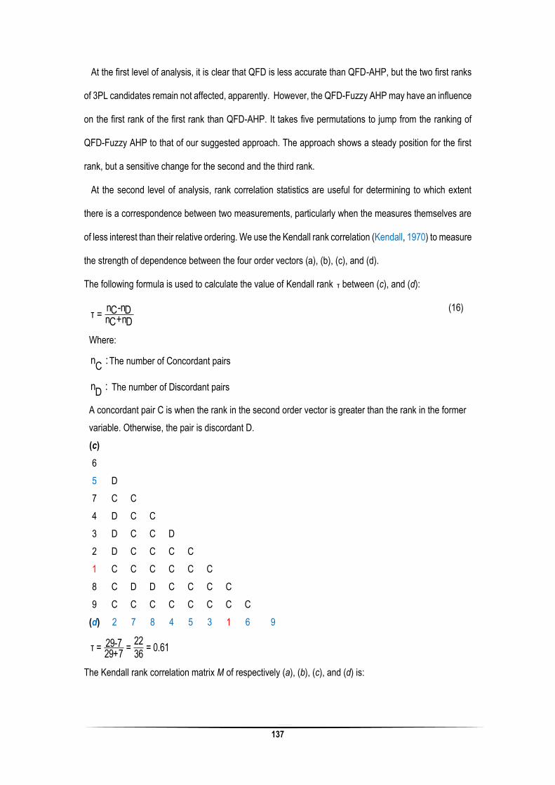
137
At the first level of analysis, it is clear that QFD is less accurate than QFD-AHP, but the two first ranks
of 3PL candidates remain not affected, apparently. However, the QFD-Fuzzy AHP may have an influence
on the first rank of the first rank than QFD-AHP. It takes five permutations to jump from the ranking of
QFD-Fuzzy AHP to that of our suggested approach. The approach shows a steady position for the first
rank, but a sensitive change for the second and the third rank.
At the second level of analysis, rank correlation statistics are useful for determining to which extent
there is a correspondence between two measurements, particularly when the measures themselves are
of less interest than their relative ordering. We use the Kendall rank correlation (Kendall, 1970) to measure
the strength of dependence between the four order vectors (a), (b), (c), and (d).
The following formula is used to calculate the value of Kendall rank τ between (c), and (d):
n -nC Dτ = n +nC D
(16)
Where:
n :C
The number of Concordant pairs
n :D The number of Discordant pairs
A concordant pair C is when the rank in the second order vector is greater than the rank in the former
variable. Otherwise, the pair is discordant D.
(c)
6
5 D
7 C C
4 D C C
3 D C C D
2 D C C C C
1 C C C C C C
8 C D D C C C C
9 C C C C C C C C
(d) 2 7 8 4 5 3 1 6 9
2229-7τ = = = 0.6129+7 36
The Kendall rank correlation matrix M of respectively (a), (b), (c), and (d) is:
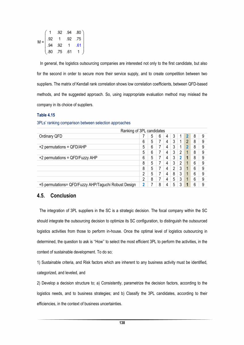
138
1 .92 .94 .80
.92 1 .92 .75M =
.94 .92 1 .
.80 .75 .61 1
61
In general, the logistics outsourcing companies are interested not only to the first candidate, but also
for the second in order to secure more their service supply, and to create competition between two
suppliers. The matrix of Kendall rank correlation shows low correlation coefficients, between QFD-based
methods, and the suggested approach. So, using inappropriate evaluation method may mislead the
company in its choice of suppliers.
Table 4.15
3PLs’ ranking comparison between selection approaches
Ranking of 3PL candidates
Ordinary QFD 7 5 6 4 3 1 2 8 9
6 5 7 4 3 1 2 8 9
+2 permutations = QFD/AHP 5 6 7 4 3 1 2 8 9
5 6 7 4 3 2 1 8 9
+2 permutations = QFD/Fuzzy AHP 6 5 7 4 3 2 1 8 9
8 5 7 4 3 2 1 6 9
8 5 7 4 2 3 1 6 9
2 5 7 4 8 3 1 6 9
2 8 7 4 5 3 1 6 9
+5 permutations= QFD/Fuzzy AHP/Taguchi Robust Design 2 7 8 4 5 3 1 6 9
4.5. Conclusion
The integration of 3PL suppliers in the SC is a strategic decision. The focal company within the SC
should integrate the outsourcing decision to optimize its SC configuration, to distinguish the outsourced
logistics activities from those to perform in-house. Once the optimal level of logistics outsourcing in
determined, the question to ask is ‘‘How’’ to select the most efficient 3PL to perform the activities, in the
context of sustainable development. To do so;
1) Sustainable criteria, and Risk factors which are inherent to any business activity must be identified,
categorized, and leveled, and
2) Develop a decision structure to; a) Consistently, parametrize the decision factors, according to the
logistics needs, and to business strategies; and b) Classify the 3PL candidates, according to their
efficiencies, in the context of business uncertainties.

139
The selected 3PL is not the most effective candidate to satisfy the logistics needs, but the most efficient
one, which achieves the real logistics needs by tacking into account the resource limitations (e.g. budget
of buyer and capacities of 3PL suppliers), and by considering extra resources to mitigate the risk factors.
We provide all the factors required to perform the 3PL selection for inbound, outbound, and reverse
logistics outsourcing. We suggest a DEA method to shorten the list of candidates after receiving
applications of the call for tender. We were inspired from the optimization of products and industrial
process, to transfer the Taguchi Robust Design technique to optimize the service processes. So, the
logistics activities being outsourced are considered as a process transforming inputs (e.g. resource and
capability criteria) to outputs (e.g. performance criteria), and submitted to a set of disturbance factors (e.g.
risk factors).
The QFD-Fuzzy AHP method is performed to consistently parametrize the decision factors, and the
appropriate Taguchi orthogonal plan leads to determine the Optimum of Taguchi; a virtual most efficient
3PL, with respect to which all the 3PL remaining in the competition are compared to. The selected 3PL
should be the closet one to the optimum of Taguchi.
The DEA-QFD/Fuzzy AHP-Taguchi Robust Design provide a consistent, and robust tool fro the problem
of supplier selection, in the context of sustainable SC, and we believe that the main contribution of this
paper is the integration of one of the most powerful tool of quality engineering in the field of selection
problems (e.g. suppliers, equipment…). This approach does not require sophisticated decision supports,
but only a commercial software to run DEA programming models, and a shift of Microsoft excel to perform
both QFD-Fuzzy AHP, and Taguchi experiments in a suitable orthogonal plan.
The suggested approach still presents some limitations to improve in furthers researches: 1) The
selection criteria should be adapted, leveled in suitable settings according to the industry sectors. Our
criteria and their settings are inspired from some recent empirical studies; 2) The negative correlations
between logistics requirements, between criteria, and between risk factors were no considered in QFD-
Fuzzy AHP, and this may consecutively, influence the weights of evaluation; and 3) the most critical
drawback is related to the difficulty to measure accurately the efficiency of a service process. The
technical efficiency as a rational function of linear combinations remains a preliminary modelling, and

140
needs to be refined in the sense of considering the complex interaction between the factors in the context
of sustainable development process.
Table 4.12
Orthogonal Plan of Taguchi: The L32b vs L9 complete parameter design layout
Risk factors
K r1 0.37 1 1 1 5 5 5 9 9 9
L r2 0.11 1 5 9 1 5 9 1 5 9
M r3 0,13 1 5 9 5 9 1 1 9 5
N r4 0.39 1 5 9 9 1 5 5 9 1
Sustainable Criteria Efficiency & Loss function of Taguchi
R
u
n
(n)
A B
C
D
E F G
H
I
J
M1
E = . En nkk=1M
NM1 1SNR =-10.log . + 20.log Enn 2M n=1m=1 Enm
Standard factor
w1 w2 w3 w4 w5 w6 w7 w8 w9 w10
.11 .09 .10 .09 .13 .09 .12 .11 .10 .06 Enm En SNRn
1 7 9 9 9 9 9 3 3 3 3 .19 .13 .10 .10 .13 .11 .11 .08 .11 .12 0.52
2 7 9 7 7 7 7 5 5 5 5 .36 .24 .19 .18 .23 .21 .20 .15 .20 .44 5.65
3 7 9 5 5 5 5 7 7 7 7 .59 .38 .28 .28 .36 .32 .30 .22 .30 .34 9.33
4 7 9 3 3 3 3 9 9 9 9 .92 .55 .40 .39 .52 .45 .42 .31 .43 .49 12.33
5 7 7 9 9 7 7 7 7 9 9 .54 .37 .29 .28 .35 .32 .30 .23 .30 .33 9.36
6 7 7 7 7 9 9 9 9 7 7 .56 .39 .30 .29 .37 .33 .31 .24 .32 .35 9.70
7 7 7 5 5 3 3 3 3 5 5 .37 .23 .16 .16 .21 .19 .17 .13 .18 .20 4.68
8 7 7 3 3 5 5 5 5 3 3 .40 .25 .18 .18 .23 .20 .19 .14 .19 .22 5.40
9 7 5 9 7 5 3 3 5 7 9 .46 .30 .22 .22 .28 .25 .23 .18 .24 .26 7.21
10 7 5 7 9 3 5 5 3 9 7 .49 .32 .23 .23 .30 .27 .25 .19 .25 .28 7.70
11 7 5 5 4 9 7 7 9 1 5 .51 .33 .25 .25 .31 .28 .26 .20 .27 .29 8.16
12 7 5 4 5 7 9 9 7 5 1 .54 .35 .26 .26 .33 .29 .27 .21 .28 .31 8.61
13 7 3 9 7 4 5 7 9 5 1 .55 .35 .26 .26 .33 .29 .28 .21 .28 .31 8.63
14 7 3 7 9 5 4 9 7 1 5 .55 .35 .26 .26 .33 .29 .27 .20 .28 .31 8.54
15 7 3 5 4 7 9 1 5 9 7 .49 .32 .23 .23 .30 .26 .25 .18 .25 .28 7.67
16 7 3 3 5 9 7 5 3 7 9 .47 .31 .23 .22 .29 .25 .24 .18 .24 .27 7.37
17 5 9 9 3 9 3 5 7 5 7 .55 .34 .25 .25 .32 .28 .26 .19 .27 .30 8.23
18 5 9 7 5 7 5 3 9 3 9 .45 .30 .22 .22 .28 .25 .23 .18 .24 .26 7.19
19 5 9 5 7 5 7 9 3 9 3 .52 .34 .25 .25 .32 .29 .27 .20 .27 .30 8.39
20 5 9 3 9 3 9 7 5 7 5 .51 .33 .25 .24 .31 .28 .26 .20 .26 .29 8.13
21 5 7 9 3 7 5 9 3 7 5 .51 .33 .25 .25 .31 .28 .26 .20 .27 .29 8.17
22 5 7 7 5 9 3 7 5 9 3 .52 .34 .25 .25 .32 .28 .27 .20 .27 .30 8.32
23 5 7 5 7 3 9 5 7 3 9 .49 .31 .23 .23 .30 .26 .24 .18 .25 .28 7.61
24 5 7 3 9 5 7 3 9 5 7 .50 .32 .24 .23 .30 .27 .25 .19 .25 .28 7.78
25 5 5 9 5 5 9 5 9 9 5 .58 .38 .28 .28 .36 .32 .30 .23 .30 .34 9.34
26 5 5 7 3 3 7 3 7 7 3 .50 .31 .22 .22 .29 .25 .24 .17 .24 .27 7.30
27 5 5 5 9 9 5 9 5 5 9 .54 .36 .27 .27 .34 .30 .28 .21 .29 .32 8.85
26 5 5 3 7 7 3 7 3 3 7 .46 .29 .21 .20 .27 .24 .22 .16 .22 .25 6.64
29 5 3 9 5 3 7 9 5 3 7 .56 .35 .25 .25 .33 .29 .27 .20 .27 .31 8.46
30 5 3 7 3 5 9 7 3 5 9 .52 .33 .24 .24 .31 .27 .25 .19 .26 .29 7.86
31 5 3 5 9 7 3 5 9 7 3 .51 .34 .25 .25 .32 .28 .26 .20 .27 .30 8.25
32 5 3 3 7 9 5 3 7 9 5 .53 .34 .25 .25 .32 .28 .26 .20 .27 .30 8.20
Opt 5 3 3 3 3 3 9 9 9 9 1.1 .63 .43 .43 .58 .50 .46 .33 .47 .55 13.1
A 1 5 5 7 9 3 5 9 7 3 5 .56 .36 .26 .26 .34 .30 .28 .21 .28 .31 8.66
A 2 5 5 5 5 9 7 5 5 9 5 .49 .32 .24 .24 .30 .27 .25 .19 .26 .29 7.91
A 3 5 5 5 5 7 9 5 5 7 7 .49 .32 .23 .23 .30 .26 .25 .19 .25 .28 7.69
A 4 7 5 7 9 5 7 7 7 5 7 .50 .34 .25 .25 .32 .28 .27 .20 .27 .30 8.31
A 5 7 5 7 9 9 5 7 7 7 5 .49 .33 .25 .25 .31 .28 .26 .20 .27 .29 8.27
A 6 7 3 9 7 9 7 7 7 7 7 .51 .35 .26 .26 .33 .29 .28 .21 .28 .31 8.64
A 7 7 7 7 7 7 7 7 9 5 7 .52 .35 .27 .26 .33 .30 .28 .21 .29 .31 8.80
A 8 5 4 5 5 5 5 5 7 5 5 .56 .34 .24 .24 .32 .28 .26 .19 .26 .30 8.09
A 9 5 5 3 7 3 3 5 3 3 5 .43 .25 .18 .18 .23 .20 .19 .14 .19 .22 5.35
A14 7 5 7 7 7 7 3 5 5 5 .34 .22 .17 .17 .21 .19 .18 .14 .18 .20 4.83

141
References
Aguezzoul A., 2014. Third Party Logistics Selection Problem: A literature review on criteria & methods.
Omega. 49 (C), 69–78.
Akao Y., Mazur G. H., 2003. The leading edge in QFD: Past, present and future. International Journal of
Quality and Reliability Management. 20 (1), 20-35.
Ameknassi L., Ait-Kadi D., Rezg N., 2016. Integration of Logistics Outsourcing Decisions in a Green Supply
Chain Design: A Stochastic Multi-Objective Multi-Period Multi-Product Programming Model. International
Journal of Production Economics, 182 (c), 165-184.
Anderson E. J., Coltman T., Devinney T. M., Keating B., 2011. What Drives the Choice of a Third-Party
Logistics Provider? Journal of Supply Chain Management, 47 (2), 97-115.
Akman G., 2015. Evaluating suppliers to include green supplier development programs via fuzzy c-means
and VIKOR methods. Comput. Ind. Eng. 86 (C), 69–82.
Awasthi A., Chauhan S. S., & Goyal S.K., 2011. A fuzzy multi-criteria approach for evaluating environmental
performance of suppliers. International Journal of Production Economics,126 (2) 370–378.
Bai C., & Joseph Sarkis J.,2010. Integrating sustainability into supplier selection with grey system and rough
set methodologies. International Journal of Production Economics, 126 (1) 252–264.
Bansal A., & Kumar P., 2013. Third Party Logistics Selection, using Hybrid Model for AHP-PROMETHHE. Int.
J. Services and Operations Management, 14 (3), 373-393.
Bask A. H., 2001. Relationships among TPL providers and members of supply chains: A Strategic
Perspective. Journal of Business & Industrial Marketing, 16 (6), 470-486.
Blanco E.E., & Craig A.J., 2009. The Value of Detailed Logistics Information in Carbon Footprint. MIT Center
for Transport & Logistic; Cambridge MA, USA; http://6ctl.mit.edu/research
Bunyaratavej K., Hahn E. D., Doh J. P., 2007. International offshoring of services: A parity study. Journal of
International Management 13 (1), 7–21.
Bhutta K.S. & Huq F., 2002. Supplier selection problem: a comparison of the total cost of ownership and
analytic hierarchy process approaches. Supply Chain Management: An International Journal. 7 (3), 126-
35.
Coltman T., Devinney T. M., Keating B., 2011. Best-Worst Scaling Approach to Predict Customer Choice for
3PL Services. Journal Business Logistics. 32 (2), 139-152
Chan L. K. & Wu M. L., 2005. A systematic approach to quality function deployment with a full illustrative
example. Omega, 33, 119-139.
Charnes A., Cooper W. W., Rodes E., 1978. Measuring the efficiency of decision making units. European
Journal of Operations Research. 2 (6), 429-444.
Chen Y., Wang T., & Wu C., 2011. Strategic decisions using the fuzzy PROMETHEE for IS outsourcing.
Expert System with Applications, 38 (10), 13216–13222
142
Dargi A., Anjomshoae A., Rahiminezhad Galankashi A., Memari A., Masine Binti Md. T. M., 2014. Supplier
Selection: A Fuzzy-ANP Approach. Procedia Computer Science. 31, 691 – 700.
Efendigil T., Önüt S., Kongar E., 2008. A holistic approach for selecting a third-party reverse logistics provider
in the presence of vagueness. Computers & Industrial Engineering, 54 (2), 269-287.
Evangelistia P., Huge-Brodin M., Isaksson K., Sweeney E., 2011.The Impact of 3PL’s Green Initiatives on
the Purchasing of Transport and Logistics Services: An Exploratory Study Vision 20/20 - Preparing today
for tomorrow’s challenges. Proceedings of the 20th International Purchasing and Supply Education and
Research Association (IPSERA) Conference, Maastricht University, pp.1-15.
Farrell M. J., 1957. The Measurement of Productive Efficiency. Journal of the Royal Statistical Society. Series
A (General), 120 (3), 253-290.
Flynn B.B., Huo B., Zhao X., 2010. The impact of supply chain integration on performance: a contingency
and configuration approach. Journal of Operations Management.28 (1), 58–71.
Franceschini F., & Rafele C., 2000. Quality evaluation in Logistics services. International Journal of Agile
Management Systems 2 (1), 49–53.
Frøkjær E., Hertzum M., Hornbæk K., 2000. Measuring usability: Are effectiveness, efficiency, and
satisfaction really correlated. In Proceedings of the ACM CHI 2000 Conference on Human Factors in
Computing Systems, ACM Press, New York. Preprint version. pp. 345-352.
Graf M., Mudambi S. M., 2005. The outsourcing of IT-enabled business processes: a conceptual model of
the location decision. Journal of International Management. 11 (2), 253–268.
Hamdan A., Rogers K. J., 2008. Evaluating the efficiency of 3PL logistics operations. International Journal
of Production Economics, 113 (1), 235–244.
Hätönen J. & Eriksson T., 2009. 30+ years of research and practice of outsourcing – Exploring the past
and anticipating the future. International Journal of Management; 15 (2), 142–155.
Ho W., Ting He T., Lee C.K.M., Emrouznejad A., 2012. Strategic logistics outsourcing: An integrated QFD
and fuzzy AHP approach. Expert Systems with Applications, 39(12), 10841–10850.
Ho W., Xu X. & Dey P. K., 2010. Multi-criteria decision making approaches for supplier evaluation and
selection: A literature review. European Journal of Operational Research. 202 (1), 16-24.
Hosseini S., & Barker K., 2016. A Bayesian network model for resilience-based supplier selection.
International Journal of Production Economics,180, 68–87.
Hsiao H.I., Kemp R.G., Vander Vorst J.G., Onno-Omta S.W., 2010. Classification of logistics outsourcing
levels and their impact on service performance: Evidence from the food processing industry. International
Journal of Production Economics, 124 (1), 75–86.
Jayant A., Gupta P., Garg S.K., Khan M., 2014. TOPSIS-AHP Based Approach for Selection of Reverse
Logistics Service Provider: A Case Study of Mobile Phone Industry. Procedia Engineering 97, 2147 –
2156
Jayaram J. & Tan K-C., 2010. Supply chain integration with third-party logistics providers. International
Journal of Production Economics, 125 (2), 261–271.

143
Jüttner U., 2005. Supply chain risk management: Understanding the business requirements from a
practitioner perspective, The International Journal of Logistics Management, 16 (1), 120 – 141.
Karimi H., Rezaeian A., 2014. Supplier selection using revised multi-segment goal programming model.
International Journal of Advanced Manufacturing technology 70 (5), 1227–1234.
Karpak B., Kumcu E., Kasuganti R.R., 2001. Purchasing materials in the supply chain: Managing a multi-
objective task. European Journal of Purchasing and Supply Management 7 (3), 209–216.
Karsak E. E., & Dursun M., 2014. An integrated supplier selection methodology incorporating QFD and
DEA with imprecise data. Expert Systems with Applications 41 (16), 6995–7004
Kendall M., 1970. Rank Correlation Methods. Griffin, London, UK, fourth edition.
Kuo R.J., Lin Y.J., 2012. Supplier selection using analytic network process and data envelopment analysis.
International Journal of Production Research, 50(11), 2852-2863.
Kwong C. K. & Bai H., 2002. A fuzzy AHP approach to the determination of importance weights of customer
requirements in Quality Function Deployment, Journal of Intelligent Manufacturing, 13, pp. 367- 377.
Langley J. Jr. & Cap Gemini, 2013. The State of Logistics Outsourcing: Results and Findings of the 17th
Annual Study. Third-Party Logistics Study, Cap Gemini consulting, 1– 40. http://www.capgemini-
consulting.com
Langley J. Jr. & Cap Gemini, 2014. The State of Logistics Outsourcing: Results and Findings of the 17th
Annual Study. Third-Party Logistics Study, Cap Gemini consulting, 1– 56. http://www.capgemini-
consulting.com
Langley J. Jr. & Cap Gemini, 2015. The State of Logistics Outsourcing: Results and Findings of the 19th
Annual Study. Third-Party Logistics Study, Cap Gemini consulting, 1– 63. http://www.capgemini-
consulting.com
Lee K. H & Kim J. W., 2009. Current status of CSR in the realm of supply management: The case of the
Korean electronics industry. Supply Chain Management: An International Journal, 14(2), 138-148.
Lee A. R., 1999. Application of modified fuzzy AHP method to analyze bolting sequence of structural joints.
UMI dissertation service. A bell & Howell company
Li X. & Olorunniwo F., 2008. An exploration of Reverse Logistics Practices in three companies. Supply
Chain Management: An International Journal. 13 (5), 381-386.
Lieb, K. Lieb, R., 2010. Environmental sustainability in the third-party logistics (3PL) industry. International
Journal of Physical Distribution and Logistics Management. 40 (7), 524-533.
Mahdiloo, M., Farzipoor Saen, R., Lee, K.-H., 2015. Technical, environmental and eco-efficiency
measurement for supplier selection: an extension and application of data envelopment analysis. Int. J.
Prod. Econ. 168, 279–289.
McGinnis M.A., Kochunny, C.M., and Ackerman K.B., 1995. Third party logistics choice, The International
Journal of Logistics Management, 6 (2), 93-102.
Meade L., Sarkis J., 2002. A conceptual model for selecting and evaluating third-party reverse logistics
providers. Supply Chain Management: An International Journal. 7 (5), 283-295.

144
Osterwalder A., 2004. The Business Model Ontology: A proposition in a Design Science Approach, Doctoral
Thesis in École des Hautes Études Commerciales. Lausanne University.
Phadke M. S., 1989. Quality Engineering using Robust Design, Prentice Hall, Englewood Cliffs, New Jersy.
Presley A., Meade L. & Sarkis J., 2007. A strategic sustainability justification methodology for organizational
decisions: A reverse logistics illustration. International Journal of Production Research, 45(18-19), 4595-
4620.
Rajesh R., Pugazhendhi S. & Muralidharan C., 2011. AQUA: Analytical model for evaluation and selection of
Third-Party Logistics service provider in supply chain. International Journal of Services and Operations
Management, 8 (1), 27-45.
Saaty T. L., 1980. The Analytic Hierarchy Process. McGraw-Hill, New York.
Sarkis J., Helms M. M. & Hervani A. A., 2010. Reverse Logistics and Social Sustainability. Corporate Social
Responsibility and Environmental Management. 17, pp. 337-354.
Savaskan R. C., Bhattacharya S. & Van Wassenhove L. N., 2004. Closed-loop supply chain models with
product remanufacturing. Management Science. 50 (2), 239–252.
Schniederjans M. J., Schniederjans A. M., Schniederjans D. G., 2015. Outsourcing & Insourcing in an
International Context. 2nd edition. Routldge,Tayor & Francis Group. ISBN 0-7656-1585-X. London & New
York.
Serrato M. A., Ryan S. M., Gaytan J., 2007. A Markov decision model to evaluate outsourcing in reverse
logistics. International Journal of Production Research, 45 (18-19), 4289-4315.
Seuring S., & Müller M., 2008. From a literature review to a conceptual framework for sustainable supply
chain management. Journal of Cleaner Production 16 (15), 1699–1710.
Sheffi Y., 2005. The Resilience Enterprise: Overcoming Vulnerability for Competitive Enterprise. MIT Press,
Cambridge, MA.
Sink H. L. & Langley C. J. JR., 1997. A Managerial Framework for the Acquisition of Third-Party Logistics
Services. Journal of Business Logistics, 18 (2), 163-189
Srivastava S. K., 2008. Network design for reverse logistics. Omega: The international Journal of
Management Science. 36 (4), 535-548.
Sullivan W. E., & Ngwenyama O. K., 2005. How are Public Sector Organizations Managing Outsourcing
Risks? An Analysis of Outsourcing Guidelines from Three Jurisdictions, Journal of Computer Information
Systems, 45:3, 73-87
Taguchi G., Chowdhury S., Taguchi S., 2000. Robust Engineering: Learn How to Boost Quality While
Reducing Costs and Time to Market. McGraw-Hill: New York,
Vahdani B., Jabbari A. H. K., Roshanaei V., & Zandieh M., 2010. Extension of the ELECTRE method for
decision-making problems with interval weights and data. International Journal of Advanced
Manufacturing Technology, 50(5–8), 793–800.
Wharton, 2012. From fringe to mainstream: Companies integrate CSR initiatives into everyday business.
Retrieved from;

145
http://knowledge.wharton.upenn.edu/article/from-fringe-to-mainstream- companies-integrate-csr-
initiatives-into-everyday-business/
Wittstruck D. & Teuteberg F., 2011.Towards a holistic approach for Sustainable Partner Selection in the
Electrics and Electronics Industry. IFIP Advances in Information and Communication Technology, Vol.
366, p. 45-69.
Wolf C., Seuring S., 2010. Environmental impacts as buying criteria for third party logistical services,
International Journal of Physical Distribution & Logistics Management, 40(1): 84-102.
Wu H-J. & Dunn S. C., 1995. Environmentally responsible logistics systems. International Journal of Physical
Distribution & Logistics Management, Vol. 25 (2), 20 – 38
Wysk R. A., Niebel B. W., Cohen P. H., and Simpson T. W., 2000. Manufacturing Processes: Integrated
Product and Process Design, McGraw Hill, New York.
Yan J., Chaudhry P. E., and Chaudhry S. S., 2003. A model of a decision support system based on case-
based reasoning for third-party logistics evaluation, Expert systems: The International Journal of
Knowledge Engineering and Neural Networks, 20 (4), 196-207.
Yang Q., & Zhao X. 2016. Are logistics outsourcing partners more integrated in a more volatile environment?
International Journal of Production Economics. 171 (2), 211–220.
Zadeh L. A., 1965. Fuzzy sets. Information and Control, 8, pp. 338-35
Zhang Y., Tao F., Laili Y., Hou B., Lv L., Zhang L., 2013. Green partner selection in virtual enterprise based
on Pareto genetic algorithms. Int. J. Adv. Technol. 67, 2109–2125

146
Chapter 5:
General Conclusion
In “Sustainable” SCs, environmental and social criteria need to be fulfilled by the members to remain
within the SCs, while it is expected that competitiveness would be maintained through meeting
heterogeneous customer needs, securing supplies, and related economic criteria. The Sustainable SC
building goes through the design of a climate change resilient SC design, completed with an effective
design for environment of products, and the activation of environmental & social practices between the
actors of the global SC. So, to build its Sustainable SC, the Focal Company FC within the SC should
integrate its customers, and notably its suppliers in the process of sustainable development. However,
the effective integration of suppliers goes through an optimum, out of which adverse implications may
affect the performance of the SC. Third Party Logistics service providers (3PLs) as particular suppliers,
possess the potentials to activate sustainable practices between different actors of the SC, expect that
the FC must determine their optimal level of integration to achieve the expected sustainable
performances, and also must select the most efficient one to promote the concepts of sustainable
development. The thesis has developed a two-stage stochastic modelling approach to help the FC
determining not only the optimal level of 3PL within the climate change resilient SC, but also the optimal
plan of Low Carbon Reduction investment for counteracting the uncertain carbon policies. The thesis has
developed also a robust integrated approach to select the most efficient 3PL to perform the outsourced
logistics, which have been defined strategically by the two-stage stochastic approach.
5.1. Contribution of the thesis
The contribution of this thesis may be enumerated into ten points:
1) The high degree of realism, scope, and complexity characterizing the suggested two-stage
modelling approach for designing a climate change resilient SC;

147
2) The suggestion of a first stochastic plan to capture uncertainty of demand, quality & quantity of
returned products, and the logistics costs;
3) The suggestion of three constructive models for roughly estimating the freight transportation,
warehousing, and reprocessing costs, and their corresponding GHG emissions of in-sourcing &
outsourcing;
4) The introduction of the internal carbon price, as a criterion to provide a normative decision
concerning the best Pareto optimal green SC configuration, integrating 3PLs, rather than a
constructive decision such as multi-criteria analysis;
5) The suggestion of a second stochastic plan to capture the uncertainty of carbon policy, in the
context of a voluntary disclosure carbon regime;
6) The consideration of a set of potential Low Carbon Reduction technologies of both Medium and
Heavy Duty Vehicles, to construct the second-stage stochastic model;
7) The consideration of the logistics activities being outsourced, as a business process
transforming resources & capabilities into capacity & performances
8) The consideration of risks factors in the outsourcing process, in addition to others selection
factors.
9) The transfer of Taguchi Robust Design from industrial process optimization to service process
optimization
10) The demonstration of the power of the selection approach DEA-QFD/fuzzy AHP/Taguchi Robust
Design comparably with the most popular selection methods.
5.2. Limitation of the thesis
We record also ten sensitivities within the suggested approaches, which should be taken back in further
researches, as follows:
a) Considering the different issues of SC management, and capturing the uncertainty of some
parameters increase significantly the model’s size. Thereby the time of data development, is
affected so much.

148
b) Although we use special logistics reviews such as Cap Gemini consulting, American
Transportation Research Institute, and European Commission - Mobility and Transport DG –
Library, to construct the computing logistics costs models and corresponding GHG emission
models, other studies per industry sectors are of great utility to compare real economical, and
environmental performances of logistics operations, between private operators and 3PL services
providers.
c) Integrating logistics outsourcing decisions in the SC network design increases the model
complexity by making quadratic the multi-objective function, thus affects the time of resolution.
d) Solving the model with an algorithm based on Epsilon-constraint approach guarantees the
convergence towards Pareto optimal solutions, but the diversity of these solutions closely
depends on the desired number of the solutions. Other evolutionary algorithms should be
implemented to improve the quality of model solving.
e) The second-stage stochastic model considers only the LCR technologies of freight
transportation, but should be extended to other energy efficiencies approaches related to bio-
fuel utilization, and related to warehousing & material handling;
f) The stochastic plan of carbon price establishment, in the context of voluntary carbon disclosure
regime, remains open to a lot of improvements, because the volatile nature of carbon prices,
and the type of industry sector;
g) The operational management of empty back hauls may lead to develop more effective
transportation itineraries, and more effective transportation schedules. So, the evolution of
heterogeneous fleet size may be subject to serious modifications, which affect the optimality of
the second-stage model.
h) The selection criteria should be adapted, leveled in suitable settings according to the industry
sectors. Our criteria and their settings are inspired from some recent empirical studies;
i) The negative correlations between logistics requirements, between criteria, and between risk
factors were no considered in QFD-Fuzzy AHP, and this may consecutively, influence the
weights of evaluation; and

149
j) the most critical drawback of the selection approach is related to the difficulty to measure
accurately the efficiency of a service process. The technical efficiency as a rational function of
linear combinations remains a preliminary modelling, and needs to be refined in the sense of
considering the complex interaction between the factors in the context of sustainable
development process.
5.3. Perspectives
In next few months, we shall address the limitation points c) & d), by focusing on the solving dimension
of the suggested two-stage stochastic modelling approach. Within the case study of microwave oven
company, the Dynamic Particle Swarm Optimization will be applied as a multi-agent parallel search
technique to relocate the global optima of the first stage model (60 nodes, 57 871 decision variables).
The convergence & dispersion of optimal SC configurations will be compared to those of the Epsilon
constraint method. Relevant managerial insights related the logistics outsourcing & Low Carbon
Reduction investment decisions, will be synthesized for building of a climate change resilient SC, in the
context of voluntary disclosure Carbone regime.

150