Swift Machine Learning Model Serving Scheduling:A Region Based Reinforcement Learning ApproachHeyang Qin

University of Nevada, Reno

Reno, NV

heyang_qin@nevada.unr.edu

Lei Yang

University of Nevada, Reno

Reno, NV

leiy@unr.edu

Request

Request

Request

Op. Op.

Op. Op.

Op.

Op.

Operation

Th. Th. Th.

Th. Th.

Request Operation Thread

Request parallelism Inter-op parallelism Intra-op parallelism

Request

Figure 1: Different parallel computing implementation for machine learn-

ing serving on CPU.

Parallel Batch Threads

Batch Size

Batch timeout

Requests

Figure 2: Configurations that can indirectly change the parallelism for

machine learning serving on GPU.

for High Performance Computing, Networking, Storage, and Analysis (SC ’19),November 17–22, 2019, Denver, CO, USA. ACM, New York, NY, USA, 14 pages.

https://doi.org/10.1145/3295500.3356164

1 INTRODUCTION1.1 MotivationRecent years have witnessed the success of machine learning in a

variety of applications in areas of vision [17, 20, 35], speech [19, 24],

and natural language [9]. Such success has prompted the develop-

ment of Machine-Learning-as-a-Service (MLaaS) [49] that provides

model training and model inference supports in the cloud. In the

model training phase, ML models are crafted and trained using

large amounts of data in an iterative manner. Then, the trained

models are deployed in serving mode to provide various inference

ABSTRACTThe success of machine learning has prospered Machine-Learning-

as-a-Service (MLaaS) – deploying trained machine learning (ML) models in cloud to provide low latency inference services at scale. To meet latency Service-Level-Objective (SLO), judicious paral-

lelization at both request and operation levels is utterly important. However, existing ML systems (e.g., Tensorflow) and cloud ML serving platforms (e.g., SageMaker) are SLO-agnostic and rely on users to manually configure the parallelism. To provide low latency ML serving, this paper proposes a swift machine learning serving scheduling framework with a novel Region-based Reinforcement Learning (RRL) approach. RRL can efficiently identify the optimal parallelism configuration under different workloads by estimat-

ing performance of similar configurations with that of the known ones. We both theoretically and experimentally show that the RRL approach can outperform state-of-the-art approaches by finding near optimal solutions over 8 times faster while reducing inference latency up to 79.0% and reducing SLO violation up to 49.9%.

CCS CONCEPTS

Permission to make digital or hard copies of all or part of this work for personal or classroom use is granted without fee provided that copies are not made or distributed for profit or commercial advantage and that copies bear this notice and the full citation on the first page. Copyrights for components of this work owned by others than ACM must be honored. Abstracting with credit is permitted. To copy otherwise, or republish, to post on servers or to redistribute to lists, requires prior specific permission and/or a fee. Request permissions from permissions@acm.org.

SC ’19, November 17–22, 2019, Denver, CO, USA© 2019 Association for Computing Machinery.

ACM ISBN 978-1-4503-6229-0/19/11. . . $15.00https://doi.org/10.1145/3295500.3356164

KEYWORDSModel Inference, machine-learning-as-a-service (MLaaS), paral-

lelism parameter tuning, reinforcement learning, workload sched-

uling, service-level-objective (SLO)

ACM Reference Format:Heyang Qin, Syed Zawad, Yanqi Zhou, Lei Yang, Dongfang Zhao, and Feng Yan. 2019. Swift Machine Learning Model Serving Scheduling: A Region Based Reinforcement Learning Approach. In The International Conference

• Computing methodologies → Reinforcement learning; • Computer systems organization → Cloud computing; • The-ory of computation;

Yanqi Zhou

Google Brain

Mountain View, CA yanqiz@google.com

Feng Yan

University of Nevada, Reno Reno, NV

fyan@unr.edu

Syed Zawad

University of Nevada, Reno Reno, NV

szawad@nevada.unr.edu

Dongfang Zhao

University of Nevada, Reno Reno, NV

dzhao@unr.edu

SC ’19, November 17–22, 2019, Denver, CO, USA Heyang Qin, Syed Zawad, Yanqi Zhou, Lei Yang, Dongfang Zhao, and Feng Yan

Intra-op=1,Service Parallelism=3

1 5 10Inter-op Parallelism

0

2000

4000

6000

8000

10000La

tenc

y(m

s)

Figure 3: Tensorflow serving performance under different parallelism

configurations for Inception V3 model running on CPU. Appropriate paral-

lelism improves system performance yet excessive parallelism decreases it

because of interference. This observation is consistent with previous study

[69]. Experimental setup is detailed in Section 6.1.

services, such as image classification [28], language processing and

translation [39], photo search [50] and captioning [67], and drug

discovery [48]. In this paper, we focus on providing low latency

model inference (a.k.a machine learning serving). Compared with

model training that targets at maximizing throughput (i.e., an offline

process tries to iterate over all training samples as fast as possi-

ble, which may take hours or even days), one main requirement

of machine learning serving is to achieve consistently low latency

to attract and retain users (i.e., serves user requests in real-time).

However, different from traditional serving applications, machine

learning models with good performance for many challenging tasks

are often containing billions of neural connections, and may take

seconds or even minutes (due to both processing time and queu-

ing waiting time) to fulfill users’ requests [76] when executed in a

sequential manner, resulting in unacceptably long latency or even

making these applications non-shippable (due to latency SLO vi-

olation). However, typical SLOs of MLaaS in production system

require 500-800ms [23, 69, 70, 74].

To satisfy the needs of MLaaS for meeting the low latency Ser-

vice Level Objective (SLO), a natural and promising approach is to

parallelize computation [17, 20]. Parallelization is especially useful

for machine learning, because most underlying operations in these

models are vector-matrix multiplications or matrix-matrix multipli-

cations [13]. Running modern machine learning systems on CPU

based infrastructure, parallelization usually have two levels [76].

At the request level, requests can be executed in parallel, which

is noted as request parallelism. Each request is usually composed

of many operations, so at the operation level, computation can

be further parallelized as inter-op parallelism (multiple operations

running simultaneously) and intra-op parallelism (each operation

utilizes multiple threads). Fig. 1 illustrates these three parallel im-

plementations. Hardware accelerator based infrastructure has its

own parallelization configuration. We use GPU as an example in

this paper, where the internal parallelism such as thread blocks

and scheduling partitions are controlled by the hardware sched-

ulers and are difficult to control directly through software-based

approaches [64]. However, there are several user defined param-

eters that can indirectly impact the parallelization performed by

GPU hardware scheduler. As shown in Fig. 2, the user defined

1 104 7

10

7

4

1Inte

r-op

para

llelis

m

Arrival rate 1 - global view

2 53 4

9

8

7

6Inte

r-op

para

llelis

m

Worst

Bestrequest parallelism request parallelism

Arrival rate 1 - local zoom in view

Figure 4: Latency under the arrival rate of 14 requests per second on

CPU with different parallel configurations (intra-op parallelism is set to 10)

using Inception V3 deployed in Tensorflow Serving. The lighter the color,

the lower the latency. The left plot shows a global performance view of

configurations and the right plot is the zoomed in view of the performance in

a small region of configurations. The coarse-grained plot shows the latency

is quite versatile globally while the zoomed-in fine-grained plot shows the

latency is smooth locally (i.e., the neighboring points in the heatmap).

1 2 3 4 5 6 7 8 9 10batch thread

5045403530252015105

batc

h tim

eout

(ms)

Arrival rate 2 - global view

1 2 3 4 5batch thread

4039383736353433323130

batc

h tim

eout

(ms)

Arrival rate 2 - local zoom in view Worst

Best

Figure 5: Latency under the arrival rate of 61 requests per second on GPU

with different parallel configurations (batch size is set to 50) using Inception

V3 model deployed in Tensorflow Serving. The lighter the color, the lower

the latency. Left plot shows a global performance view of configurations and

the right plot is the zoomed in view of the performance in a small region of

configurations.

Batch Size and Batch Timeout (i.e., maximum wait time allowed to

form the target batch size) together determines the input dimen-

sions, which impacts hardware scheduling decisions such as how

the scheduler allocates and dispatches thread blocks and also how

warp scheduler schedules warps into scheduling partitions. The

Parallel Batch Threads can also impact the parallelism decisions

of the GPU hardware scheduler. In machine learning serving sys-

tems, each parallel implementation and each related configuration

becomes a control knob. Parallelism configuration has significant

impact on system performance. As indicated in Fig. 3, a well-tuned

parallelism configuration can boost system performance up to 10

times compared to sequential execution (e.g., running Inception V3

on CPU infrastructure).

Machine learning serving is usually interactive and latency sensi-

tive [23, 69] compared with model training or HPC workload which

is usually throughput-oriented (i.e., SLO-agnostic). Compared with

traditional web service, ML-serving usually involves hundreds to

thousands of operations with complex correlation among them [5],

which makes it challenging to model in a white-box manner. This

makes machine learning serving an unique workload that is chal-

lenging to breakdown and do fine-tuning at operation level. How to

Swift Machine Learning Model Serving Scheduling:A Region Based Reinforcement Learning Approach SC ’19, November 17–22, 2019, Denver, CO, USA

0 2 4 6 8 10 12 14Difference in configurations

0

50

100

150

200

250

300

Diff

eren

ce in

per

form

ance

Figure 6: Difference in performance v.s. difference in configuration. The

difference in configurations is calculated by their Euclidean distance.

optimally control these knobs depends on the performance require-

ment, workload characteristic, and available computing resources,

which becomes an important yet challenging problem.

Parallelism configuration tuning has recently garnered much at-

tention [7, 30]. However, existing methods require domain specific

information and techniques to tune the parallelism configuration

(see the detailed discussion in Section 2), which may not be appli-

cable to many machine learning applications. Recently, Feng et al.proposed SERF in [69, 70] to achieve optimal parallelism configu-

ration for machine learning serving using an analytical queuing

model, which is applicable for exponential arrival process and ho-

mogeneous request size in certain image classification applications.

For many other applications (such as video, speech, and natural lan-

guage processing), the arrival process may not be exponential, and

request sizes may be heterogeneous. In addition, SERF supports

only request level parallelism and CPU-based hardware. There-

fore, there is a pressing need to develop a novel approach that can

support two levels of parallelisms and hardware accelerators like

GPU to effectively and efficiently tune parallelism configuration

for machine learning applications with diverse arrival processes

and heterogeneous request sizes.

1.2 ChallengesIt is challenging to tune parallelism configuration in modern ma-

chine learning serving systems. For CPU-based infrastructure, the

configuration space is relatively large due to the two-level paral-

lelism. Fig. 4 illustrates request latency under only two parallelism

configurations with fixed intra-op parallelism. Even for two paral-

lelisms on a machine with only 10 cores, there are many parallelism

configurations. The similar observation holds for GPU-based infras-

tructure, see Fig 5. For GPU, the search space is even larger due to

the wider range of configuration parameters (e.g., Batch Timeout

alone can have hundreds to thousands possible choices). In addition,

due to the indirect impact of configuration parameters in the GPU

case, it is very difficult to model or predict the behaviors. Worse still,

the optimal parallelism configuration is also very sensitive to the

load. In Fig. 4, even with a slight change in load, the latency distri-

bution (note the latency here is composed of both service time and

queuing waiting time) under different parallelism configurations

becomes quite different, which significantly increases the search

space and prohibits exhaustive search. Moreover, it is worth noting

that the high computation and memory needs of machine learning

models can result in complex interference behavior among parallel

computation [69, 70], which is less a problem in model training that

focuses on the overall throughput rather than the processing speed

of individual request. Such non-linear performance behavior of

different configurations brings significant challenges for profiling

and analytical modeling [36, 71].

In addition, modern machine learning models usually contain

thousands to tens of thousands of operations with complex depen-

dencies, which may result in the state-of-the-art modeling tech-

niques [69, 70] ineffective. Moreover, the workload and system en-

vironment in many machine learning applications are often highly

dynamic [16, 73], which requires the scheduling policy with an

agile adaptive ability, in order to meet the sensitive latency SLO

[23, 42]. In this case, traditional learning-based methods [36], re-

quiring a large training set and a long convergence time, can hardly

be applicable to machine learning model serving. Therefore, swift

deployment is required for most online serving systems, which can

learn the dynamics of the workload and system environment and

optimize the model performance in an online manner.

1.3 Summary of Main ContributionsIn this paper, we propose a swift machine learning serving sched-

uling framework to solve the above challenges. The proposed frame-

work is driven by a lightweight region-based reinforcement learning

(RRL) approach that can efficiently identify the optimal configu-

ration under different workloads. Like previous studies [32, 45],

we formulate our problem as Markov Decision Process. The key

insight is that the system performances under different similar con-

figurations in a region can be accurately estimated by using the

system performance under one of these configurations, due to their

similarity (see Fig. 6). This key finding motivates us to develop RRL

that can speedup the learning process by orders of magnitude faster

than state-of-the-art deep reinforcement learning methods with

very limited training data. We theoretically show that this speedup

increases with the size of the region, which, however, would result

in a performance gap between the RRL and the optimal solution

due to the estimation error. Thanks to the unique structure of our

problem (see Fig. 6), we are able to choose a suitable size of the

region such that the learning speed can be significantly improved

with near optimal performance.

We prototype the proposed framework on top of the popular Ten-

sorflow Serving [44] machine learning serving system and support

both CPU and GPU based hardware infrastructure. We release the

source code for public access.1We conduct extensive experimental

evaluations on both CPU and GPU clusters and the results show

that by continuously learning the new traffic patterns and updating

the scheduling policies, RRL can quickly adapt to the ever-changing

dynamics of workloads and system environments. Compared to the

state-of-the-art reinforcement learning methods, RRL can reduce

the average latency up to 79.0% on CPU-based infrastructure and up

to 69.3% on GPU-based infrastructure compared to state-of-the-art

approaches DeepRM[38] and CAPES[37]. In the SLO-aware sce-

nario, RRL can offer SLO guarantee even under strict targets and

provide up to 49.9% SLO violation reduction compared to CAPES

and up to 43.4% compared to DeepRM. In addition, the proposed

1https://github.com/SC-RRL/RRL

SC ’19, November 17–22, 2019, Denver, CO, USA Heyang Qin, Syed Zawad, Yanqi Zhou, Lei Yang, Dongfang Zhao, and Feng Yan

framework does not have assumptions on workload or underlying

systems and thus can be used for most modern machine learning

systems and applications.

2 BACKGROUND AND RELATED WORK2.1 Machine Learning ServingMachine learning has recently shown a great success on important

yet challenging artificial intelligence applications, such as vision,

speech, and natural language. How to efficiently deploy trained

machine learning models in serving (or sometimes called inference

or model serving) mode to provide low latency services has drawn

great attention in both academia and industry [18, 69, 70, 75]. Major

public cloud service providers like Google, Amazon, and Microsoft

all provide MLaaS to facilitate users to publish their models and

provide online services. Several machine learning serving systems

have been open-sourced recently [10, 18, 44], among which the

most widely used one is Tensorflow Serving [44]. In this paper, we

use Tensorflow Serving as a case study system to implement and

evaluate the proposed framework.

Hardware acceleration [14, 46] has been used to accelerate the

computation in machine learning serving by using customized hard-

ware such as GPUs, FPGAs, and ASICs. Software techniques such

as model compression and simplification [27] have also successfully

improved the latency of machine learning serving through reducing

computation time and storage space by trading off some accuracy.

In addition, recent work using compiler techniques [3] and accel-

eration library [1] have also shown good results in accelerating

machine learning serving. All the above techniques are comple-

mentary to our scheduling framework and can be combined with

our work to achieve better results as all of them use parallelization

techniques and have tuning parameters for optimal performance.

In addition, the proposed framework does not rely on any specific

models or underlying systems or hardware.

Another promising technique for reducing the latency of ma-

chine learning serving is parallelism as most operations in machine

learning models are vector-matrix multiplications or matrix-matrix

multiplications [13] that can be efficiently parallelized. Request par-allelism, inter-op parallelism, and intra-op parallelism are the typical

ways to parallel computation on CPU in today’s machine learning

serving systems. On GPU, computation is parallelized through SMs

and scheduling partitions, though difficult to control through soft-

ware mechanisms, it can be indirectly adjusted through batching

parameters such as batch size, batch threads, and batch timeout. Toachieve efficient parallelism, it is critical to understand the behav-

ior of different configurations. As discussed in the introduction,

existing methods [7, 15, 30, 69, 70] either require domain specific

information and techniques to tune the parallelism configuration or

are applicable for special arrival process with homogeneous request

size in certain applications. To achieve a more general solution, we

aim to design a scheduling framework that can work with general

user traffic patterns and system environments on both CPUs and

GPUs based infrastructure.

2.2 Interactive ServingMachine learning serving is not the first application utilizing paral-

lelism to reduce latency. Actually, parallelism has been widely used

in many online services for the similar purpose. Here we focus on

interactive serving systems that utilize parallelism to accelerate

processing or share resources among users’ requests. There is a line

of work in the literature studying adaptive resource allocation for

requests sharing the same server systems [25, 47]. However, they

consider only request level parallelism. Raman et al. develop an

API and runtime system for parallelism orchestration [47], but they

assume requests do not interfere with each other, which does not

hold for computation-intensive machine learning serving. Haque etal. observe large variability on interactive services and propose in-

cremental parallelization approach to achieve optimal latency [25],

which is not suitable for machine learning serving workload due

to the large number of operations and complex dependencies. An-

other line of work [7, 15, 30] relies on domain knowledge of specific

applications and/or the special architecture of specific systems to

guide the optimization of parallel configurations. Dazhao et al. de-sign an adaptive scheduling for Spark Streaming [15]. Jeon et al.propose an analytical algorithm to compute the optimal parallelism

based on their characterization results of web search queries [30].

Alipourfard et al. build performance models using Bayesian Opti-

mization for cloud configuration with the focus of recurring big

data analytics [7]. None of these work investigates the unique char-

acteristics of machine learning workloads and tailor the parallelism

scheduling methodology accordingly.

2.3 Parameter Tuning using ReinforcementLearning

Reinforcement learning [22, 56, 59, 68] was first proposed in 1940s

and has been widely used in different applications. Here we focus

on the application of system parameter tuning using reinforce-

ment learning. Mao et al. propose reinforcement learning based

resource management method for multi-resource cluster schedul-

ing problem [38]. Li et al. develop a reinforcement learning based

parameter tuning system for storage systems [37]. Both work use

traditional point-based reinforcement learning and suffer from slow

convergence and adaptivity. Mirhoseini et al. propose to optimize

Tensorflow operation placement between CPU and GPU using long

short-term memory (LSTM), which is applicable for only CPU-GPU

co-design architecture [41]. In this paper, we develop a new region-

based reinforcement learning based on the unique characteristics

of machine learning serving performance behavior to significantly

improve the convergence speed and the agility in dynamic environ-

ment.

2.4 Workload SchedulingMany works have studied the job scheduling problem in HPC clus-

ter. Baskaran et al. [12] proposed a model based parameter tuning

method for applications across GPUs. Isaila et al. [29] proposeda heuristic algorithm to schedule I/O parallel jobs in a decentral-

ized manner for filesystems. Krishnamoorthy et al. [34] proposeda framework that can automatically optimize application memory

placement in parallel systems by block-sparse arrays. In the record-

breaking HPC cluster built by Sakagami et al. [53], the parallelismis manually tuned. For ML-serving, different serving models, work-

loads, and system environments can lead to very different perfor-

mance characteristics. Thus the approaches of modeling, heuristic

and white-box tuning are infeasible for machine learning serving.

Swift Machine Learning Model Serving Scheduling:A Region Based Reinforcement Learning Approach SC ’19, November 17–22, 2019, Denver, CO, USA

3 RRL-BASED SCHEDULING FRAMEWORKIn this section, we present the RRL-based scheduling framework for

machine learning serving. The RRL-based scheduling framework

is designed to dynamically adjust the parallelism configuration of

machine learning serving systems based on dynamic system load,

in order to optimize system performance (e.g., response latency or

resource consumption). As illustrated in Fig. 4, system performance

varies under different parallelism configurations even for the same

load, and the relationship among the system performance, paral-

lelism configurations, and system load is challenging to capture in

a closed form. To tackle this challenge, the proposed framework

leverages a learning approach to find the optimal parallelism con-

figuration. Specifically, the proposed framework consists of three

main components: 1) profiler, 2) scheduler, and 3) region-based

reinforcement learning, as illustrated in Fig. 7. The profiler collects

various system characteristics, such as the current user traffic load

and the corresponding system performance (e.g., average latency or

resource consumption) under this load and the present parallelism

configuration. The scheduler then adjusts the parallelism configu-

ration for the measured load level based on the current scheduling

policy. At the same time, the region-based reinforcement learning

dynamically updates the scheduling policy based on the measured

system load and corresponding performance, in order to adapt to

the system dynamics.

1) Profiler. The profiler measures the system load (i.e., request

arrival rate) and the latency (also known as response time) of each

request. Latency is used to measure the system performance. Mean-

while, the profiler also collects hardware-related information (such

as CPU core number, CPU utilization, available GPUs, GPU utiliza-

tion, and network statistics). All these information can be used to

optimize the system performance for a specific scheduling objective.

2) Scheduler. The scheduler adjusts the parallelism configuration

based on the current system load, scheduling policies, and hardware

information such as the availability of resource.

3) Region-based reinforcement learning. As the core of the pro-posed framework, the region-based reinforcement learning compo-

nent aims to find the optimal scheduling policy and quickly adjust

the scheduling policy to adapt to the system dynamics. Specifically,

the reward function in Fig. 7 first calculates the value of the system

objective function using the system performance measured by the

profiler, and then the learning component learns the scheduling

policy based on this observed reward. One key challenge is that the

learning process would be significantly long if the scheduling policy

is incrementally improved in a point-by-point learning manner. To

address this challenge, the proposed region-based reinforcement

learning can speedup this learning process by leveraging the key

feature of the system as illustrated in Fig. 6. It is observed that

the system performances under different similar configurations are

similar. Based on this feature, the system performance under one

configuration can be used to estimate the system performances

under other similar configurations, which would significantly re-

duce the number of samples needed to learn the optimal scheduling

policy. For example, if we choose the radius of the configuration

region equal to 2, then we can use a single observation to update all

configurations in this region and obtain a roughly 10 times faster

Request

Runtime Information

SchedulingPolicy

Update

Configuration

Reward

Respond

Profiler

Machine LearningServingServer

Client

Load

Region-based Reinforcement Learning

State

RewardFunction

Performance

Training

RRL-based Scheduling Framework

Scheduling

Figure 7: Overview of RRL-based scheduling framework.

convergence with limited performance loss due to the estimation

error. The detailed design is presented in Section 4.

4 REGION-BASED REINFORCEMENTLEARNING

In this section, we propose a region-based reinforcement learning

(RRL) approach, in order to speedup the learning process of the

scheduling policy. Specifically, we first formulate the machine learn-

ing serving scheduling as a Markov Decision Process (MDP), and

then theoretically show that the RRL approach can achieve a near

optimal solution with fast convergence speed.

4.1 ML Serving Scheduling: A MDP ViewThe objectives of machine learning serving scheduling are 1) to

minimize response latency using a given amount of resources [31,

47] or 2) to minimize resource consumption while meeting latency

SLO. Both objectives are supported in our scheduling framework

[40, 77]. In the interest of space, we focus on the first objective of

minimizing response latency.

Let s ∈ S denote the overall load level (i.e., system state), where

S denotes the set of possible load levels. The parallelism configu-

ration (i.e., system action) c ∈ C is denoted as a tuple of request

parallelism cservice, inter-op parallelism c inter, and intra-op paral-

lelism c intra, i.e., c = (cservice, c inter, c intra), where C denotes the

set of possible parallelism configurations. For machine learning

serving, latency can vary under different loads (system states) for

the same parallelism configuration [69], which is challenging to

characterize in a closed form. However, the average request latency

r (s, c) under the system state s and the parallelism configuration ccan be measured as reward. In this paper, we assume that the sched-

uler has no apriori knowledge of system state transitions, except

the Markov property (i.e., the state transition depends on only the

previous state)2. Under this model, the machine learning serving

scheduling is cast as aMarkov Decision Process, aiming to minimize

2Markov models are often used to model the workload dynamics, e.g., [45] verifies the

Markov property for different applications. In our application, the Markov property

SC ’19, November 17–22, 2019, Denver, CO, USA Heyang Qin, Syed Zawad, Yanqi Zhou, Lei Yang, Dongfang Zhao, and Feng Yan

Point-based Perception Region-based Perception

Observed Latency Estimated Latency Unknown Latency

Figure 8: Point-based vs. region-based learning. The RRL approach can

more efficiently learn the latency under different configurations.

the expected cumulative discounted latency E[∑∞t=0 γ

t rt (st , ct )],where γ ∈ (0, 1] is a discount factor and rt (st , ct ) denotes the la-tency observed at time t under system state st and parallelism

configuration ct .At each time t , the scheduler chooses a parallelism configuration

based on a policy, defined as π : π (s, c) → [0, 1], where π (s, c) isthe probability that configuration c is used in state s . To find the

optimal policy, the Q-learning method can be applied. However,

the convergence of the Q-learning method is slow, especially when

the space of state-configuration pairs is large. One key reason for

this slow convergence is that it searches the space point by point

and incrementally improving the policy. Though many approaches

[11, 21, 63] have been proposed to improve the convergence speed,

they are still point-based learning essentially, and would not be

applicable to our problem with large state-configuration space as

shown in our experiments in Section 6.

4.2 RRL: From Point-based to Region-basedLearning

To speedup the learning process, we propose the RRL approach.

The key idea is that when observing the latency r (s, c), we will esti-mate the latency in a region with configurations close to c under thisstate s , and then use the estimated latency in this region to learn thepolicy, as illustrated in Fig. 8. Intuitively, this region-based learning

approach would significantly improve the learning speed if a large

region is used. However, the converged policy may deviate from the

optimal one, due to the potential estimation errors of the latency

associated with the region such that the larger the region is, the

larger the potential errors would be. Obviously, there is a trade-off

between the learning speed and the optimality of the policy, which

intimately depends on the size of the region and the latency esti-

mation scheme. When the region degenerates to a single point, the

RRL approach would degenerate to the traditional reinforcement

learning approaches. In this paper, Euclidean distance is used to

measure the distance between two configurations since both CPU

and GPU configurations are numeric, see Fig. 9. Note that other

similarity measures can also be applied in RRL.

Specifically, the RRL approach consists of two main components:

1) latency estimation based perception and 2) policy update.

4.2.1 Latency estimation based perception. Let Qt (st , ct ) denotethe perception of the expected cumulative discounted latency under

is also satisfied. The experiments in Section 6 also corroborate the correctness of the

Markov model in our application.

c2

2

4

8 10

6

serv

ice

para

llelis

m

8

c1

Euclidean Distance

6

intra-op

8

inter-op

6

10

4 42 2

Figure 9: An example of Euclidean distance between two configurations

c1 and c2, i.e.,√(c service

1− c service

2)2 + (c inter

1− c inter

2)2 + (c intra

1− c intra

2)2.

state st and configuration ct . Define the region around ct as C(ct ) ={c | | |c − ct | | ≤ δ ,∀c ∈ C}, where δ ≥ 0 denotes the size of the

region. Using the observed latency rt (st , ct ), the latency under

other configurations in C(ct ) can be estimated as

rt (st , c) = f (c, rt (st , ct )),∀c ∈ C(ct ), (1)

where f : C × R+ → R+ is the latency estimation function and

f (ct , rt (st , ct )) = rt (st , ct ). Based on (1), we update the perception

of the expected cumulative discounted latency in the region by

∀c ∈ C(ct ), Qt+1(st , c) = (1 − αt )Qt ((st , c) + αt (rt (st , c)+γ min

c ∈CQt (st+1, c)),

(2)

where αt ∈ [0, 1] is the learning rate. As is standard, the learning

rate is assumed to satisfy

∑∞t=1 αt = ∞ and

∑∞t=1 α

2

t < ∞. The

perceptions of other configurations (c < C(ct )) will remain the

same, i.e., Qt+1(st , c) = Qt (st , c),∀c < C(ct ).4.2.2 Policy update. Based on the perceptions, we can use the

Boltzmann distribution [4] to update the policy for state st

πt (st , c) =exp(−βQt (st ,c))∑c∈C exp(−βQt (st , c))

,∀c ∈ C, (3)

where β ≥ 0 controls the exploration-exploitation trade-off. When

β is very small, the scheduler would explore the space randomly;

when β is large, the scheduler would tend to exploit the configura-

tion with the lowest perceived latency.

It is worth noting that the performance of the RRL approach

hinges on the accuracy of the latency estimation (1). In practice, it is

challenging to characterize f in a closed form, due to the stochastic

nature of the state and the latency. To tackle this challenge, we im-

plement this estimation function using neural network as discussed

in Section 5. The detailed description of the RRL approach is given

in Algorithm 1.

4.3 Performance Analysis of RRLIn this section, we will analyze the convergence rate and optimality

performance of the RRL approach. To facilitate the analysis, we

assume that the estimation error of the latency estimation (1) is

upper bounded by ∆ ≥ 0 for all state-configuration pairs in the

Swift Machine Learning Model Serving Scheduling:A Region Based Reinforcement Learning Approach SC ’19, November 17–22, 2019, Denver, CO, USA

Algorithm 1 Region-based reinforcement learning

Initialization: Choose β , δ , and γ . Set t = 0 and Q0(s, c) =1/|C|, ∀c ∈ C, s ∈ S.

For each time slot t1) Choose a configuration based on the current policy πt .2) Update the perception based on (2).

3) Update the policy for the current state st based on (3).

space, i.e.,

|rt (st , c) − rt (st , c)| ≤ ∆,∀c ∈ C(ct ), st ∈ S, (4)

where rt (st , c) denotes the real latency that can be observed if the

configuration c is chosen. In (4), ∆ is intimately related to the size

of the region δ . In general, ∆ increases with δ , and ∆ becomes zero

when δ is zero.3The main results are summarized in the following

theorem.

Theorem 4.1. The RRL approach can asymptotically convergeto a near optimal solution with probability one as t goes to infin-ity. The performance gap is upper bounded by ∆

1−γ . The asymp-

totic convergence rate is O(1/(nδ t)R(1−γ )) if R(1 − γ ) < 1/2 andO(

√log log(nδ t)/(nδ t)) otherwise, where nδ denotes the number of

state-configuration pairs in the region with size δ and R denotes theratio of the minimum and maximum state-configuration selectionprobabilities.

Proof. First, we introduce an auxiliary perception process Qt (st , ct )as follows:

Qt+1(st , ct ) = (1 − αt )Qt ((st , ct ) + αt (rt (st , ct )+γ min

c ∈CQt (st+1, c)),

(5)

where Qt (st , ct ) corresponds to the learning process using the real

latency instead of the estimation (1). Then, the performance results

of the RRL approach can be obtained by comparing Qt (st , ct ) withthe optimal Q∗(st , ct ) using Qt (st , ct ). The idea is to use triangle

inequality to decompose the comparison ofQt (st , ct ) andQ∗(st , ct )

into two difference processes:

|Qt (st , ct ) −Q∗(st , ct )| ≤ |Qt (st , ct ) − Qt (st , ct )|

+|Qt (st , ct ) −Q∗(st , ct )|.(6)

Using stochastic-approximation techniques and prior convergence

results of traditional Q-learning [62], we can obtain the upper

bounds for each difference process in (6), which are summarized in

the following lemmas.

Lemma 4.2. For each time t , the difference process of Qt (st , ct )and Qt (st , ct ) satisfies |Qt (st , ct ) − Qt (st , ct )| ≤

1

1−γ ∆.

Proof. We show |Qt (st , ct ) − Qt (st , ct )| ≤1

1−γ ∆ by induction.

At t = 1, with assumption (4) for any s ∈ S and c ∈ C, we have

|Q1(s, c) −Q1(s, c)| = |α0r0(s, c) − α0r0(s, c)|

≤ |r0(s, c) − r0(s, c)| ≤ ∆ = b1∆,

where α0 ≤ 1, and b1 = 1 is less than 1/(1 − γ ) where γ ≤ 1.

3Note that ∆ also highly depends on the accuracy of the estimation function. In this

paper, a neural network based estimation function is implemented, and the error bound

is shown to be small in our experiments.

Using induction, we assume that for a given t > 1,

|Qt (s, c) −Qt (s, c)| ≤ bt∆

for any s ∈ S and c ∈ C holds, i.e., bt ≤ 1/(1 − γ ).We aim to show that bt+1 ≤ 1/(1 − γ ). At t + 1, we have

|Qt+1(st , ct ) −Qt+1(st , ct )|

=|(1 − αt )(Qt (st , ct ) −Qt (st , ct )) + αt (rt (st , ct ) − rt (st , ct )

+ γ (min

c ∈CQt (st+1, c) −min

c ∈CQt (st+1, c)))|

(a)≤ (1 − αt )|Qt (s, c) −Qt (s, c)| + αt (|rt (s, c) − rt (s, c)|

+ γ max

c ∈C|Qt (st+1, c) −Qt (st+1, c)|)

(b)≤ (1 − αt )bt∆ + αt (∆ + γbt∆)

(c)≤ (1 −

1

t)bt∆ +

1

t(∆ + γbt∆) = bt+1∆,

where (a) we apply triangle inequality and use the fact |(min Qt (st+1, c)−minQt (st+1, c)))| ≤ max |Qt (st+1, c) −Qt (st+1, c)|. (b) We use the

assumption that |Qt (s, c) − Qt (s, c)| ≤ bt∆ for any s ∈ S and

c ∈ C. (c) After some algebra, we have the coefficient of αt equal to∆(1 − bt (1 − γ )), which is positive as bt ≤ 1/(1 − γ ). Thus, it holdsfor some αt ≤ 1

t that satisfies the conditions of the learning rate.

Therefore, we have a recurrence relation

bt+1 = (1 −1

t)bt +

1

t(1 + γbt ).

By some algebra, we have the following recurrence equation:

bt+1 = (1 +γ − 1

t)bt +

1

t, b1 = 1. (7)

We can solve this recurrence equation and obtain the following

solution

bt+1 =1 −

Γ(t+γ )Γ(t+1)Γ(γ )

1 − γ, (8)

where Γ in (8) denotes the gamma function. Note that the right

hand side of (8) is a non-decreasing function of t upper boundedby

1

1−γ , i.e.,

bt+1 =1 −

Γ(t+γ )Γ(t+1)Γ(γ )

1 − γ≤

1

1 − γ. (9)

Thus, we have

|Qt (s, c) −Qt (s, c)| ≤ bt∆ ≤1

1 − γ∆, (10)

where 0 < γ < 1. This concludes the proof of Lemma 4.2. □

Lemma 4.3. For each time t , the difference process of Qt (st , ct )and Q∗(st , ct ) satisfies the following relations asymptotically withprobability one: |Qt (st , ct )−Q

∗(st , ct )| ≤ B/(nδ t)R(1−γ ) ifR(1−γ ) <

1/2 and |Qt (st , ct ) −Q∗(st , ct )| ≤ B√log log(nδ t)/(nδ t), otherwise,

where B > 0 is some constant.

Proof. The proof follows [57, 62] by generalizing the point-

based update to the region-based update. Specifically, nδ is intro-

duced to denote the number of state-configuration pairs in the re-

gion for the region-based update, while nδ = 1 for the point-based

update. The details are omitted due to the space limitation. □

SC ’19, November 17–22, 2019, Denver, CO, USA Heyang Qin, Syed Zawad, Yanqi Zhou, Lei Yang, Dongfang Zhao, and Feng Yan

As t goes to infinity, the difference process of Qt (st , ct ) andQ∗(st , ct ) converges to zero asymptotically with probability one

based on Lemma 4.3. Therefore, the performance gap is determined

by Lemma 4.2. The convergence rate can be obtained from Lemma

4.3. This concludes the proof of Theorem 4.1. □

Remarks: Theorem 4.1 confirms our intuition that the RRL ap-

proach can accelerate the convergence speed of the reinforcement

learning such that the larger nδ (i.e., the larger δ ), the faster theRRL converges. However, the fast convergence speed is at the cost

of performance loss, i.e., there would be a gap∆

1−γ between the

RRL and the optimal solution. When δ = 0, we have nδ = 1 and

∆ = 0, and the results of Theorem 4.1 degenerates to the results for

the traditional point-based reinforcement learning [62]. Thanks tothe unique structure of our problem (see Fig. 6), we are able to choosea suitable size of the region such that the convergence speed can besignificantly improved with near optimal performance (see Section6). Note that the proof of Lemma 4.3 generalizes the proof of [62]

by not only using the region-based update but also relaxing the

learning rate conditions in [62] by following [57], in order to avoid

sub-optimal solutions in the original proof of [62].

5 IMPLEMENTATIONIn this section, we discuss how we implement the proposed ap-

proach in machine learning serving systems, focusing on the design

of neural network based estimation function and the Tensorflow

Serving integration of the proposed framework.

5.1 Neural Network based Estimation FunctionAs discussed in Section 4, it is challenging to characterize the esti-

mation function in a closed form. Neural network based approaches

have shown great potentials in many applications [54, 55]. In this

paper, we propose a neural network based estimation function. One

key challenge is how to find a suitable neural network structure

for the estimation function (1) to support swift machine learn-

ing serving scheduling. If a simple network structure is used, it

may not effectively capture the structure of the underlying state-

configuration space, which may lead to high estimation error; if a

complicated network structure is used, it may take a long training

time, which is not suitable for online serving systems.

To strike a balance between complexity and efficiency, we use an

evolutionary algorithm NEAT [58] to guide the design of network

structure. The network we designed has two hidden layers (one

with 256 neurons and the other with 64 neurons) using ReLu[43]

as activation function and one output layer with linear activation,

after experimenting different network structures. In this paper, the

network parameters are optimized using Follow-the-regularized-

Leader (FTRL)[6] optimizer instead of the Adam method or other

popular optimizers [33, 72]. This is because the number of train-

ing samples in our problem is far less than the number of state-

configuration pairs in the space when doing online tuning, and

thus FTRL performs very well here. Moreover, FTRL is insensitive

to model parameters. Our experiments in Tensorflow Serving show

that FTRL performs well even where there is limited training data.

(see Section 6).

5.2 Tensorflow Serving IntegrationWe integrate the proposed scheduling framework into Tensorflow

Serving [44], a popular production-ready machine learning serving

system. While we do a case study with Tensorflow serving, nothing

prevents the proposed work being integrated with other machine

learning serving systems as we do not use anything Tensorflow

specific features. In the interest of space, we only briefly highlight

our main implementation design.

Profiler: Though TensorBoard [2] offers sophisticated visualizationand logging capabilities for training machine learning models using

Tensorflow, it provides no support for Tensorflow Serving. There-

fore, we implement a lightweight profiler that can continuously

monitor the workload and track request latency by instrumenting

the DirectSession and gRPCmodules and implementing the dispatch

queue as discussed next. In this way, the overall execution time is

split into waiting time, service time, and network delay. For GPU

monitoring, we also use NVIDIA System Management Interface

(NVIDIA-SMI) running as daemon to profile real-time GPU perfor-

mance information such as utilization. We collect request arrival

rate, real-time request latency and system resource utilization from

Tensorflow Serving. Since our framework is designed to be light-

weight and portable, we do not use hardware level integration.

Rather we rely on the metrics reported by third party software

such as Tensorflow Serving and NVIDIA-SMI. Their reported met-

rics may have error yet the nature of reinforcement learning and

the reward estimation of RRL enables our framework to be error-

tolerant, which is validated by the evaluation results in Section 6.

The metrics are reported by Profiler in real-time, so it serves as a

performance monitor for Scheduler to identify network congestion

and single-point failure in the cluster.

Scheduler: Tensorflow Serving does not support request level par-

allelism, so we implement a flexible dispatch queue that supports

plugin scheduling policies (e.g., users can specify scheduling ob-

jective such as minimizing latency, achieving SLO while minimiz-

ing resources). The dispatch queue follows the scheduling policies

from the RRL module and assigns requests to the target node with

pre-computed inter-op and intra-op parallelism. Current implemen-

tation of Tensorflow serving sets inter-op according to intra-op

parallelism. Thus we modify ModelServer to enable fine grained

control of inter-op and intra-op parallelism. The Scheduler is failure-

aware to reduce the risk of breaking SLO due to node failures.

RRL: We implement the RRL as a module that takes inputs of the

monitoring information from Profiler to compute and update sched-

uling policies and feed to the Scheduler. The RRL module allows

asynchronous neural network training to put little extra overhead

to the serving system. The neural network is trained with all previ-

ous seen samples until hitting either the training step or training

loss threshold.

6 EXPERIMENTAL EVALUATIONIn this section, we conduct extensive experimental evaluation to

verify the effectiveness and robustness of the proposed RRL-based

scheduling framework using a rich selection of state-of-the-art

machine learning applications on both CPU and GPU based infras-

tructure. We first evaluate the sensitivity of RRL in convergence

speed by adjusting the region size. Then we compare RRL with the

Swift Machine Learning Model Serving Scheduling:A Region Based Reinforcement Learning Approach SC ’19, November 17–22, 2019, Denver, CO, USA

Number of Tasks

Inception

ResNetV2

DeepSpeech0

2000

4000

6000

8000

10000

Ope

ratio

ns

0 500 1000 1500 2000Service Time (ms)

0

0.2

0.4

0.6

0.8

1

Cum

ulat

ive

Dis

tribu

tion

Func

tion Distribution of Workload Duration

InceptionResNetV2DeepSpeech

Figure 10: The number of tasks and the distribution of request duration

of service workloads measured on CPU infrastructure.

latest reinforcement learning approaches in the following aspects:

(i) effectiveness in terms of minimizing latency; (ii) robustness in

dynamic workload; (iii) strict SLO guarantee; (iv) effectiveness of

meeting SLO while minimizing resource usage.

6.1 Experimental SetupMachine Learning Serving System: We prototype RRL based

scheduling framework and integrate it in Tensorflow Serving, refer

to Section 5.2 for more details.

Service Workloads: We use three popular machine learning ap-

plications for evaluation:

• Inception V3 [61]: popular deep convolutional neural network

based image classification model classifies 256x256 color images

in 1,000 categories with 48 layers and tens of millions parameters.

Serving requests are from ImageNet 22K dataset [52] with homoge-

neous sizes.

• Inception ResNet V2 [60]: advanced deep convolutional neural

network based image classificationmodel with the aid of ResNet[26]

that allows network with depth of 162 layers and hundreds of

millions of parameters. Serving requests are from ImageNet 22K

dataset [52] with homogeneous sizes.

• Deep Speech V2 [8]: popular deep recurrent neural network

based speech to text model with 11 layers. Serving requests samples

are from TeD talk dataset [51] and with heterogeneous sizes.

Inception, ResNet, and Deepspeech are representative models for

Convolutional Neural Networks, Residual Neural Network, and Re-

current Neural Network, covering popular ML-serving application

domains such as computer vision and natural language processing.

The number of tasks and the request duration of servive workloads

are illustrated in Fig. 10, where the request duration of Inception

and ResNet are homogeneous while Deepspeech is heterogenous.

Arrival Process: We use two non-exponential arrival processes

for evaluation:

• WiKi: given there is no public available ML serving trace, we

opt for traces of user traffic visiting Wikipedia website [66] with

unpredictable load spikes.

• Dynamic: a synthetic dynamic arrival process composed of

periods of Poison process with randomly changing average, which

has more pronounced changes from one period to the next.

0 1 2 3 4 5 6 7 8 9 10Region Size

0

2000

4000

6000

Con

verg

ence

Spe

ed(it

erat

ion)

0

0.2

0.4

0.6

0.8

1Sensitive Analysis on Inception

0 1 2 3 4 5 6 7 8 9 10Region Size

0

1000

2000

3000

4000

5000

0

0.2

0.4

0.6

0.8

1

Pred

ictio

n Er

ror

Sensitive Analysis on DeepSpeech

Figure 11: Sensitivity analysis of RRL in terms of the convergence time

in iteration (left y-axis) and the prediction error (right y-axis) as a function

of region size using Inception and DeepSpeech.

Hardware:We use a cluster of 10 identical servers. Each of them

is equipped with dual-sockets Intel(R) Xeon(R) CPU E5-2630 v4 @

2.20GHz and four NVIDIA GeForce GTX 1080 Ti GPUs, 64 GB of

memory, and connected through Infiniband. One sever is acting as

client, one server is used as dispatch queue, and the rest are request

processing severs.

Baseline Approaches: Since there is no alternative intelligent

scheduling framework for a direct comparison, we opt to imple-

ment the state-of-the-art reinforcement learning approaches for

tuning parallelism configuration in our scheduling framework:

DeepRM [38] and CAPES [37], as they are the closest approaches

for online ML-serving scheduling. CAPES is a general-purpose

parameter tuning algorithm and DeepRM is a job scheduling algo-

rithm designed to work under limited resources. Both DeepRM and

CAPES are open-sourced, so we use their codes published at github

and set parameters according their papers [37, 38]. Specifically, in

the structure level, DeepRM uses one hidden layer of 20 neurons

and CAPES uses 2 hidden layers of 200 neurons. Both of them are

trained with RMSProp [65] with the learning rate of 0.001 according

to their original design. For fair comparison, we feed the profiling

metrics (e.g., latency and resource utilization) provided by Profiler

into the reward function and use both the profiling metrics and

rewards as the input parameters of DeepRM and CAPES to com-

pute the corresponding output parameters, which are interpreted

by the Scheduler afterwards. We assign a dedicated server to do

the reinforcement learning tasks so that the learning tasks are not

interfered with the inference tasks. Our evaluation results suggest

that our deployment of both DeepRM and CAPES is consistent with

their paper and could identify reasonably good configurations, see

Fig. 12.

SLO setting:As our testbed is not production level, we set relativelyloose SLOs in our evaluation, i.e., a range between 1800ms and

3200ms to emulate different latency requirements for ML serving

in production environments, which is consistent with previous

studies [69, 70, 74].

6.2 Convergence Speed Analysis of RRLThe key tuning parameter in RRL is the region size as it controls

the trade-off between convergence speed and accuracy. We per-

form sensitivity analysis of RRL to verify the theoretical results

SC ’19, November 17–22, 2019, Denver, CO, USA Heyang Qin, Syed Zawad, Yanqi Zhou, Lei Yang, Dongfang Zhao, and Feng Yan

0 1000 2000Time(min)

10

15

Arriv

al R

ate

(a) Arrival Process (Wiki)

0 1000 2000Time(min)

1

520

Late

ncy(

ms)

0 1000 2000Time(min)

520

Late

ncy(

ms)

(c) Latency (WiKi)DeepSpeech (CPU)

0 1000 2000Time(min)

Arriv

al R

ate

(d) Arrival Process (Dynamic) 20

15

10

0 1000 2000Time(min)

15

20

Late

ncy(

ms)

(e) Latency (Dynamic)Inception (CPU)

0 1000 2000Time(min)

15

20

Late

ncy(

ms)

(f) Latency (Dynamic)DeepSpeech (CPU)

10 210 2

10 2 10 2

(b)b) Latency (WiKi)Inception (CPU)

CAPES DeepRM RRL

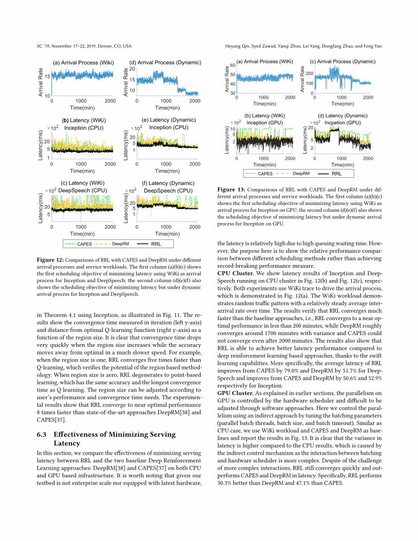
Figure 12: Comparisons of RRL with CAPES and DeepRM under different

arrival processes and service workloads. The first column (a)(b)(c) shows

the first scheduling objective of minimizing latency using WiKi as arrival

process for Inception and DeepSpeech; the second column (d)(e)(f) also

shows the scheduling objective of minimizing latency but under dynamic

arrival process for Inception and DeepSpeech.

in Theorem 4.1 using Inception, as illustrated in Fig. 11. The re-

sults show the convergence time measured in iteration (left y-axis)

and distance from optimal Q-learning function (right y-axis) as a

function of the region size. It is clear that convergence time drops

very quickly when the region size increases while the accuracy

moves away from optimal in a much slower speed. For example,

when the region size is one, RRL converges five times faster than

Q-learning, which verifies the potential of the region based method-

ology. When region size is zero, RRL degenerates to point-based

learning, which has the same accuracy and the longest convergence

time as Q learning. The region size can be adjusted according to

user’s performance and convergence time needs. The experimen-

tal results show that RRL converge to near optimal performance

8 times faster than state-of-the-art approaches DeepRM[38] and

CAPES[37].

6.3 Effectiveness of Minimizing ServingLatency

In this section, we compare the effectiveness of minimizing serving

latency between RRL and the two baseline Deep Reinforcement

Learning approaches: DeepRM[38] and CAPES[37] on both CPU

and GPU based infrastructure. It is worth noting that given our

testbed is not enterprise scale nor equipped with latest hardware,

0 1000 2000Time(min)

0

100

200

Arriv

al R

ate

(c) Arrival Process (Dynamic)

0 1000 2000Time(min)

2

5

20

Late

ncy(

ms)

(d) Latency (Dynamic)Incpetion (GPU)

0 1000 2000Time(min)

30

40

50

60

Arriv

al R

ate

(a) Arrival Process (WiKi)

0 1000 2000Time(min)

25

10

Late

ncy(

ms)

(b) Latency (WiKi)Inception (GPU) 10 2 10 2

CAPES DeepRM RRL

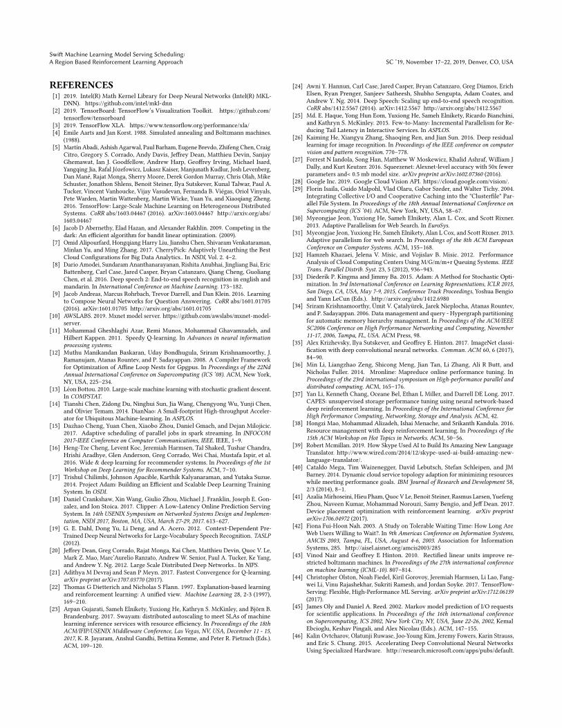
Figure 13: Comparisons of RRL with CAPES and DeepRM under dif-

ferent arrival processes and service workloads. The first column (a)(b)(c)

shows the first scheduling objective of minimizing latency using WiKi as

arrival process for Inception on GPU; the second column (d)(e)(f) also shows

the scheduling objective of minimizing latency but under dynamic arrival

process for Inception on GPU.

the latency is relatively high due to high queuingwaiting time. How-

ever, the purpose here is to show the relative performance compar-

ison between different scheduling methods rather than achieving

record-breaking performance measure.

CPU Cluster. We show latency results of Inception and Deep-

Speech running on CPU cluster in Fig. 12(b) and Fig. 12(c), respec-

tively. Both experiments use WiKi trace to drive the arrival process,

which is demonstrated in Fig. 12(a). The WiKi workload demon-

strates random traffic pattern with a relatively steady average inter-

arrival rate over time. The results verify that RRL converges much

faster than the baseline approaches, i.e., RRL converges to a near op-

timal performance in less than 200 minutes, while DeepRM roughly

converges around 1700 minutes with variance and CAPES could

not converge even after 2000 minutes. The results also show that

RRL is able to achieve better latency performance compared to

deep reinforcement learning based approaches, thanks to the swift

learning capabilities. More specifically, the average latency of RRL

improves from CAPES by 79.0% and DeepRM by 51.7% for Deep-

Speech and improves from CAPES and DeepRM by 50.6% and 52.9%

respectively for Inception.

GPU Cluster. As explained in earlier sections, the parallelism on

GPU is controlled by the hardware scheduler and difficult to be

adjusted through software approaches. Here we control the paral-

lelism using an indirect approach by tuning the batching parameters

(parallel batch threads, batch size, and batch timeout). Similar as

CPU case, we use WiKi workload and CAPES and DeepRM as base-

lines and report the results in Fig. 13. It is clear that the variance in

latency is higher compared to the CPU results, which is caused by

the indirect control mechanism as the interaction between batching

and hardware scheduler is more complex. Despite of the challenge

of more complex interactions, RRL still converges quickly and out-

performs CAPES and DeepRM in latency. Specifically, RRL performs

30.3% better than DeepRM and 47.1% than CAPES.

Swift Machine Learning Model Serving Scheduling:A Region Based Reinforcement Learning Approach SC ’19, November 17–22, 2019, Denver, CO, USA

6.4 Robustness under Dynamic WorkloadWorkload can change dynamically over time in practice, so it is

important to have swift adaptivity. In this section, we evaluate the

robustness of the proposed scheduling framework in terms of the

ability to quickly adapt to the workload change. We use a synthetic

dynamic arrival process for evaluation, as shown in Fig. 12(d), the

arrival change is more pronounced than the WiKi arrival process,

which emulates the change of user traffic patterns over time.

CPUCluster. The latency results on CPU cluster for Inception and

DeepSpeech are shown in Fig. 12(e) and Fig. 12(f), respectively. The

results suggest that RRL can adapt to the user traffic change very

quickly. Thanks to the region-based learning approach, the number

of samples that RRL needs for updating scheduling policy is far less

than point-based approaches, which leads to a much shorter adapt-

ing time compared to CAPES and DeepRM. The latency results

also show that RRL has a more stable latency performance com-

pared to deep reinforcement learning based approaches. In contrast,

DeepRM takes a much longer time to update scheduling polices and

CAPES shows significant variation due to its slow learning process.

On average, RRL reduces the latency of DeepSpeech by 69.3% and

49.2% compared to CAPES and DeepRM respectively, and 58.1% and

45.8% for Inception respectively.

GPU Cluster. We also evaluate the dynamic workload on GPU-

based infrastructure. Due to the complex interactions, a side effect

brought by indirect control, the adapt speed is slower than CPU case.

However, even in this challenging scenario, RRL still consistently

outperforms CAPES and DeepRM by 38.0% and 69.1% on average

respectively.

6.5 Meeting Strict SLOWe evaluate our approach under the scenario of meeting strict

SLO target, i.e., 95th percentile latency SLO of 550ms for CPU and

520ms for GPU.4Fig. 14 (note the logscale in both axes) demon-

strates that the CCDF latency comparison of RRL with CAPES and

DeepRM using CPU cluster and GPU cluster, respectively. Overall,

RRL achieves a much shorter tail latency compared to CAPES and

DeepRM. From the tail comparison, it is clear that RRL can provide

strict SLO guarantee and achieve up to 49.9% SLO violation reduc-

tion compared to CAPES and up to 43.4% compared to DeepRM,

thanks to its SLO-aware design.

6.6 Meeting SLO With Minimum ResourcesAnother common scheduling objective is meeting relatively loose

SLO while minimizing the resource usage (e.g., cloud environment

or shared cluster), which is also supported by our scheduling frame-

work. Fig. 15 provide a case study of this scheduling objective using

DeepSpeech, ResNet, and Inception under dynamic workload on

CPU and GPU infrastructure, respectively.

CPU Cluster. The latency of DeepSpeech over the time running

on CPU cluster using different scheduling methods is present in

Fig. 15(b), where both CAPES and DeepRM perform poorly on

achieving the SLO target. CAPES spent around 200 minutes before

finding a scheduling policy that can achieve the SLO but at the

4It is worth to emphasize again that the relative high latency is because our testbed is

not enterprise scale nor equipped with latest hardware, so both the processing time

and the queuing waiting time is relatively high.

300 500 1000 2000Latency (ms)

0.5

4.9

36.548.3100

CC

DF

(%)

(a) Latency (WiKi)Inception (CPU)

300 500 750 2000Latency (ms)

0.5

4.9

17.2

54.8100

CC

DF

(%)

(b) Latency (WiKi)Inception (GPU)

CAPES DeepRM RRL

Figure 14: Comparisons of RRL with CAPES and DeepRM under strict

SLO (95th percentile latency of 550ms for CPU and 520ms for GPU).

expense of high CPU utilization whereas DeepRM violates the

SLO whenever the workload has significant changes. RRL on the

contrast always guarantees the SLO, even during abrupt workload

changes. Another comparison is on resource utilization, which

is very important for consolidating resources and achieve cost

efficient serving. We report the CPU utilization at Fig. 15(c), where

RRL consistently consumes much less CPU resource than both

CAPES and DeepRM and provides great potential for workload

consolidation and/or cost saving, which is especially important for

serving machine learning models in cloud environment. Similar

observations holds for the ResNet results in Fig. 15(e)(f), where

all three methods achieve SLO in a short time, but RRL uses only

one fourth CPU resources compared to the deep reinforcement

learning abased methods. On average, the average CPU resources

saved by RRL for DeepSpeech is 13.4% compared to CAPES and

8.5% compared to DeepRM. For ResNet, the resource saving is even

more significant: RRL on average saved 52.9% from CAPES and

46.8% from DeepRM.

GPU Cluster.We show the GPU results in Fig. 15(h)(i), where RRL

keeps a stable latency right under SLO and only uses half GPU

resources compared with CAPES and DeepRM. On average, RRL

saved 10.6% GPU resources compared with CAPES and 12.9% GPU

resources from DeepRM. Considering the high cost of GPU, such

saving is not trivial.

6.7 DiscussionEvaluation results show that RRL outperforms the standard deep

reinforcement learning methods in both speed and accuracy, in

spite of the estimation error in RRL, when environment/workload

changes quickly. RRL uses the unique characteristics of ML-serving

to accelerate the learning process: when parallelism changes, the la-

tency is quite versatile globally while smooth locally. Othermethods

do not have such insights. When environment/workload changes,

RRLmay have already converged to a near optimal solution, whereas

other methods may be still far away. Therefore, in online systems,

RRL outperforms the standard deep reinforcement learning meth-

ods in both speed and accuracy.

7 CONCLUSION AND FUTUREWORKIn this paper, we proposed a RRL-based scheduling framework for

machine learning serving that can efficiently identify the optimal

SC ’19, November 17–22, 2019, Denver, CO, USA Heyang Qin, Syed Zawad, Yanqi Zhou, Lei Yang, Dongfang Zhao, and Feng Yan

CAPES DeepRM RRL

Figure 15: Comparisons of RRL with CAPES and DeepRM when achieving SLO while optimizing resource usage (i.e., CPU and GPU utilization) under

dynamic arrival processes and service workloads. (a)-(f) shows the scheduling objective of minimizing CPU utilization with respect to given SLOs for model

DeepSpeech and ResNet under dynamic workloads. (g)(h)(i) shows the second scheduling objective of achieving SLO while minimizing GPU usage with

Inception under dynamic arrival process. The SLOs for DeepSpeech, ResNet and Inception are 2400ms, 3200ms, and 1850ms, respectively.

configuration under dynamic workloads. A key observation is that

the system performance under similar configurations in a region

can be accurately estimated by using the system performance un-

der one of these configurations, due to their correlation, based on

which we developed the RRL approach. We theoretically showed

that the RRL approach can achieve a near optimal solution with fast

convergence speed. The proposed framework is prototyped and

evaluated on Tensorflow serving system and can be easily extended

to other machine learning serving systems. Extensive experimental

evaluation on both CPU cluster and GPU cluster show that RRL

can quickly adapt to the dynamics of workloads and system envi-

ronments. Compared to the state-of-the-art Deep Reinforcement

Learning based methods (DeepRM and CAPES), the proposed sched-

uling framework can reduce the average latency by up to 79.0% on

CPU cluster and 69.3% on GPU cluster. In the SLO-aware scenario,

RRL reduces up to 49.9% SLO violation under strict SLO require-

ment while reducing the resource usage by up to 52.9% on CPU

and 12.9% on GPU in loose SLO scenario. In addition, the proposed

solution does not have assumptions on workload or underlying

systems and thus can be used for most modern machine learning

systems and applications.

ACKNOWLEDGMENTThis work is supported in part by the following grants: National

Science Foundation CCF-1756013, IIS-1838024 (using resources pro-

vided by Amazon Web Services as part of the NSF BIGDATA pro-

gram), EEC-1801727, and Amazon Web Services Cloud Credits for

Research Award. We also acknowledge the support of Research &

Innovation and the Office of Information Technology at the Uni-

versity of Nevada, Reno for computing time on the Pronghorn

High-Performance Computing Cluster. We thank the anonymous

reviewers for their insightful comments and suggestions.

Swift Machine Learning Model Serving Scheduling:A Region Based Reinforcement Learning Approach SC ’19, November 17–22, 2019, Denver, CO, USA

REFERENCES[1] 2019. Intel(R) Math Kernel Library for Deep Neural Networks (Intel(R) MKL-

DNN). https://github.com/intel/mkl-dnn

[2] 2019. TensorBoard: TensorFlow’s Visualization Toolkit. https://github.com/

tensorflow/tensorboard

[3] 2019. TensorFlow XLA. https://www.tensorflow.org/performance/xla/

[4] Emile Aarts and Jan Korst. 1988. Simulated annealing and Boltzmann machines.

(1988).

[5] Martín Abadi, Ashish Agarwal, Paul Barham, Eugene Brevdo, Zhifeng Chen, Craig

Citro, Gregory S. Corrado, Andy Davis, Jeffrey Dean, Matthieu Devin, Sanjay

Ghemawat, Ian J. Goodfellow, Andrew Harp, Geoffrey Irving, Michael Isard,

Yangqing Jia, Rafal Józefowicz, Lukasz Kaiser, Manjunath Kudlur, Josh Levenberg,

Dan Mané, Rajat Monga, Sherry Moore, Derek Gordon Murray, Chris Olah, Mike

Schuster, Jonathon Shlens, Benoit Steiner, Ilya Sutskever, Kunal Talwar, Paul A.

Tucker, Vincent Vanhoucke, Vijay Vasudevan, Fernanda B. Viégas, Oriol Vinyals,

Pete Warden, Martin Wattenberg, Martin Wicke, Yuan Yu, and Xiaoqiang Zheng.

2016. TensorFlow: Large-Scale Machine Learning on Heterogeneous Distributed

Systems. CoRR abs/1603.04467 (2016). arXiv:1603.04467 http://arxiv.org/abs/

1603.04467

[6] Jacob D Abernethy, Elad Hazan, and Alexander Rakhlin. 2009. Competing in the

dark: An efficient algorithm for bandit linear optimization. (2009).

[7] Omid Alipourfard, Hongqiang Harry Liu, Jianshu Chen, Shivaram Venkataraman,

Minlan Yu, and Ming Zhang. 2017. CherryPick: Adaptively Unearthing the Best

Cloud Configurations for Big Data Analytics.. In NSDI, Vol. 2. 4–2.[8] Dario Amodei, SundaramAnanthanarayanan, Rishita Anubhai, Jingliang Bai, Eric

Battenberg, Carl Case, Jared Casper, Bryan Catanzaro, Qiang Cheng, Guoliang

Chen, et al. 2016. Deep speech 2: End-to-end speech recognition in english and

mandarin. In International Conference on Machine Learning. 173–182.[9] Jacob Andreas, Marcus Rohrbach, Trevor Darrell, and Dan Klein. 2016. Learning

to Compose Neural Networks for Question Answering. CoRR abs/1601.01705

(2016). arXiv:1601.01705 http://arxiv.org/abs/1601.01705

[10] AWSLABS. 2019. Mxnet model server. https://github.com/awslabs/mxnet-model-

server.

[11] Mohammad Gheshlaghi Azar, Remi Munos, Mohammad Ghavamzadeh, and

Hilbert Kappen. 2011. Speedy Q-learning. In Advances in neural informationprocessing systems.

[12] Muthu Manikandan Baskaran, Uday Bondhugula, Sriram Krishnamoorthy, J.

Ramanujam, Atanas Rountev, and P. Sadayappan. 2008. A Compiler Framework

for Optimization of Affine Loop Nests for Gpgpus. In Proceedings of the 22NdAnnual International Conference on Supercomputing (ICS ’08). ACM, New York,

NY, USA, 225–234.

[13] Léon Bottou. 2010. Large-scale machine learning with stochastic gradient descent.

In COMPSTAT.[14] Tianshi Chen, Zidong Du, Ninghui Sun, Jia Wang, Chengyong Wu, Yunji Chen,

and Olivier Temam. 2014. DianNao: A Small-footprint High-throughput Acceler-

ator for Ubiquitous Machine-learning. In ASPLOS.[15] Dazhao Cheng, Yuan Chen, Xiaobo Zhou, Daniel Gmach, and Dejan Milojicic.

2017. Adaptive scheduling of parallel jobs in spark streaming. In INFOCOM2017-IEEE Conference on Computer Communications, IEEE. IEEE, 1–9.

[16] Heng-Tze Cheng, Levent Koc, Jeremiah Harmsen, Tal Shaked, Tushar Chandra,

Hrishi Aradhye, Glen Anderson, Greg Corrado, Wei Chai, Mustafa Ispir, et al.

2016. Wide & deep learning for recommender systems. In Proceedings of the 1stWorkshop on Deep Learning for Recommender Systems. ACM, 7–10.

[17] Trishul Chilimbi, Johnson Apacible, Karthik Kalyanaraman, and Yutaka Suzue.

2014. Project Adam: Building an Efficient and Scalable Deep Learning Training

System. In OSDI.[18] Daniel Crankshaw, Xin Wang, Giulio Zhou, Michael J. Franklin, Joseph E. Gon-

zalez, and Ion Stoica. 2017. Clipper: A Low-Latency Online Prediction Serving

System. In 14th USENIX Symposium on Networked Systems Design and Implemen-tation, NSDI 2017, Boston, MA, USA, March 27-29, 2017. 613–627.

[19] G. E. Dahl, Dong Yu, Li Deng, and A. Acero. 2012. Context-Dependent Pre-

Trained Deep Neural Networks for Large-Vocabulary Speech Recognition. TASLP(2012).

[20] Jeffrey Dean, Greg Corrado, Rajat Monga, Kai Chen, Matthieu Devin, Quoc V. Le,

Mark Z. Mao, Marc’Aurelio Ranzato, Andrew W. Senior, Paul A. Tucker, Ke Yang,

and Andrew Y. Ng. 2012. Large Scale Distributed Deep Networks.. In NIPS.[21] Adithya M Devraj and Sean P Meyn. 2017. Fastest Convergence for Q-learning.

arXiv preprint arXiv:1707.03770 (2017).[22] Thomas G Dietterich and Nicholas S Flann. 1997. Explanation-based learning

and reinforcement learning: A unified view. Machine Learning 28, 2-3 (1997),

169–210.

[23] Arpan Gujarati, Sameh Elnikety, Yuxiong He, Kathryn S. McKinley, and Björn B.

Brandenburg. 2017. Swayam: distributed autoscaling to meet SLAs of machine

learning inference services with resource efficiency. In Proceedings of the 18thACM/IFIP/USENIX Middleware Conference, Las Vegas, NV, USA, December 11 - 15,2017, K. R. Jayaram, Anshul Gandhi, Bettina Kemme, and Peter R. Pietzuch (Eds.).

ACM, 109–120.

[24] Awni Y. Hannun, Carl Case, Jared Casper, Bryan Catanzaro, Greg Diamos, Erich

Elsen, Ryan Prenger, Sanjeev Satheesh, Shubho Sengupta, Adam Coates, and

Andrew Y. Ng. 2014. Deep Speech: Scaling up end-to-end speech recognition.

CoRR abs/1412.5567 (2014). arXiv:1412.5567 http://arxiv.org/abs/1412.5567

[25] Md. E. Haque, Yong Hun Eom, Yuxiong He, Sameh Elnikety, Ricardo Bianchini,

and Kathryn S. McKinley. 2015. Few-to-Many: Incremental Parallelism for Re-

ducing Tail Latency in Interactive Services. In ASPLOS.[26] Kaiming He, Xiangyu Zhang, Shaoqing Ren, and Jian Sun. 2016. Deep residual

learning for image recognition. In Proceedings of the IEEE conference on computervision and pattern recognition. 770–778.

[27] Forrest N Iandola, Song Han, Matthew W Moskewicz, Khalid Ashraf, William J

Dally, and Kurt Keutzer. 2016. Squeezenet: Alexnet-level accuracy with 50x fewer

parameters and< 0.5 mb model size. arXiv preprint arXiv:1602.07360 (2016).[28] Google Inc. 2019. Google Cloud Vision API. https://cloud.google.com/vision/.

[29] Florin Isaila, Guido Malpohl, Vlad Olaru, Gabor Szeder, and Walter Tichy. 2004.

Integrating Collective I/O and Cooperative Caching into the "Clusterfile" Par-

allel File System. In Proceedings of the 18th Annual International Conference onSupercomputing (ICS ’04). ACM, New York, NY, USA, 58–67.

[30] Myeongjae Jeon, Yuxiong He, Sameh Elnikety, Alan L. Cox, and Scott Rixner.

2013. Adaptive Parallelism for Web Search. In EuroSys.[31] Myeongjae Jeon, Yuxiong He, Sameh Elnikety, Alan L Cox, and Scott Rixner. 2013.

Adaptive parallelism for web search. In Proceedings of the 8th ACM EuropeanConference on Computer Systems. ACM, 155–168.

[32] Hamzeh Khazaei, Jelena V. Misic, and Vojislav B. Misic. 2012. Performance

Analysis of Cloud Computing Centers Using M/G/m/m+r Queuing Systems. IEEETrans. Parallel Distrib. Syst. 23, 5 (2012), 936–943.

[33] Diederik P. Kingma and Jimmy Ba. 2015. Adam: A Method for Stochastic Opti-

mization. In 3rd International Conference on Learning Representations, ICLR 2015,San Diego, CA, USA, May 7-9, 2015, Conference Track Proceedings, Yoshua Bengioand Yann LeCun (Eds.). http://arxiv.org/abs/1412.6980

[34] Sriram Krishnamoorthy, Ümit V. Çatalyürek, Jarek Nieplocha, Atanas Rountev,

and P. Sadayappan. 2006. Data management and query - Hypergraph partitioning

for automatic memory hierarchy management. In Proceedings of the ACM/IEEESC2006 Conference on High Performance Networking and Computing, November11-17, 2006, Tampa, FL, USA. ACM Press, 98.

[35] Alex Krizhevsky, Ilya Sutskever, and Geoffrey E. Hinton. 2017. ImageNet classi-

fication with deep convolutional neural networks. Commun. ACM 60, 6 (2017),

84–90.

[36] Min Li, Liangzhao Zeng, Shicong Meng, Jian Tan, Li Zhang, Ali R Butt, and

Nicholas Fuller. 2014. Mronline: Mapreduce online performance tuning. In

Proceedings of the 23rd international symposium on High-performance parallel anddistributed computing. ACM, 165–176.

[37] Yan Li, Kenneth Chang, Oceane Bel, Ethan L Miller, and Darrell DE Long. 2017.

CAPES: unsupervised storage performance tuning using neural network-based

deep reinforcement learning. In Proceedings of the International Conference forHigh Performance Computing, Networking, Storage and Analysis. ACM, 42.

[38] Hongzi Mao, Mohammad Alizadeh, Ishai Menache, and Srikanth Kandula. 2016.

Resource management with deep reinforcement learning. In Proceedings of the15th ACM Workshop on Hot Topics in Networks. ACM, 50–56.

[39] Robert Mcmillan. 2019. How Skype Used AI to Build Its Amazing New Language

Translator. http://www.wired.com/2014/12/skype-used-ai-build-amazing-new-

language-translator/.

[40] Cataldo Mega, Tim Waizenegger, David Lebutsch, Stefan Schleipen, and JM

Barney. 2014. Dynamic cloud service topology adaption for minimizing resources

while meeting performance goals. IBM Journal of Research and Development 58,2/3 (2014), 8–1.

[41] AzaliaMirhoseini, Hieu Pham, Quoc V Le, Benoit Steiner, Rasmus Larsen, Yuefeng

Zhou, Naveen Kumar, Mohammad Norouzi, Samy Bengio, and Jeff Dean. 2017.

Device placement optimization with reinforcement learning. arXiv preprintarXiv:1706.04972 (2017).

[42] Fiona Fui-Hoon Nah. 2003. A Study on Tolerable Waiting Time: How Long Are

Web Users Willing to Wait?. In 9th Americas Conference on Information Systems,AMCIS 2003, Tampa, FL, USA, August 4-6, 2003. Association for Information

Systems, 285. http://aisel.aisnet.org/amcis2003/285

[43] Vinod Nair and Geoffrey E Hinton. 2010. Rectified linear units improve re-

stricted boltzmann machines. In Proceedings of the 27th international conferenceon machine learning (ICML-10). 807–814.

[44] Christopher Olston, Noah Fiedel, Kiril Gorovoy, Jeremiah Harmsen, Li Lao, Fang-

wei Li, Vinu Rajashekhar, Sukriti Ramesh, and Jordan Soyke. 2017. TensorFlow-

Serving: Flexible, High-Performance ML Serving. arXiv preprint arXiv:1712.06139(2017).

[45] James Oly and Daniel A. Reed. 2002. Markov model prediction of I/O requests

for scientific applications. In Proceedings of the 16th international conferenceon Supercomputing, ICS 2002, New York City, NY, USA, June 22-26, 2002, Kemal

Ebcioglu, Keshav Pingali, and Alex Nicolau (Eds.). ACM, 147–155.

[46] Kalin Ovtcharov, Olatunji Ruwase, Joo-Young Kim, Jeremy Fowers, Karin Strauss,

and Eric S. Chung. 2015. Accelerating Deep Convolutional Neural Networks

Using Specialized Hardware. http://research.microsoft.com/apps/pubs/default.

SC ’19, November 17–22, 2019, Denver, CO, USA Heyang Qin, Syed Zawad, Yanqi Zhou, Lei Yang, Dongfang Zhao, and Feng Yan

aspx?id=240715

[47] Arun Raman, Hanjun Kim, Taewook Oh, Jae W. Lee, and David I. August. 2011.

Parallelism orchestration using DoPE: the degree of parallelism executive. In

Proceedings of the 32nd ACM SIGPLAN Conference on Programming LanguageDesign and Implementation, PLDI 2011, San Jose, CA, USA, June 4-8, 2011. 26–37.

[48] Bharath Ramsundar, Steven Kearnes, Patrick Riley, Dale Webster, David Konerd-

ing, and Vijay Pande. 2015. Massively Multitask Networks for Drug Discovery.

arXiv preprint arXiv:1502.02072 (2015).[49] Mauro Ribeiro, Katarina Grolinger, andMiriamAMCapretz. 2015. Mlaas:Machine

learning as a service. In 2015 IEEE 14th International Conference on MachineLearning and Applications (ICMLA). IEEE, 896–902.

[50] Chuck Rosenberg. 2019. Improving Photo Search: A Step Across the Semantic

Gap. http://googleresearch.blogspot.com/2013/06/improving-photo-search-step-

across.html.

[51] Anthony Rousseau, Paul Deléglise, and Yannick Esteve. 2014. Enhancing the

TED-LIUM Corpus with Selected Data for Language Modeling and More TED

Talks.. In LREC. 3935–3939.[52] Olga Russakovsky, Jia Deng, Hao Su, Jonathan Krause, Sanjeev Satheesh, SeanMa,

ZhihengHuang, Andrej Karpathy, Aditya Khosla, Michael Bernstein, Alexander C.

Berg, and Li Fei-Fei. 2015. ImageNet Large Scale Visual Recognition Challenge.

International Journal of Computer Vision (IJCV) 115, 3 (2015), 211–252.[53] Hitoshi Sakagami, Hitoshi Murai, Yoshiki Seo, and Mitsuo Yokokawa. 2002. 14.9

TFLOPS three-dimensional fluid simulation for fusion science with HPF on the

Earth Simulator. In Proceedings of the 2002 ACM/IEEE conference on Supercomput-ing, Baltimore, Maryland, USA, November 16-22, 2002, CD-ROM, Roscoe C. Giles,

Daniel A. Reed, and Kathryn Kelley (Eds.). IEEE Computer Society, 21:1–21:14.

http://ieeexplore.ieee.org/xpl/mostRecentIssue.jsp?punumber=10618

[54] John Schulman, Philipp Moritz, Sergey Levine, Michael Jordan, and Pieter Abbeel.

2015. High-dimensional continuous control using generalized advantage estima-

tion. arXiv preprint arXiv:1506.02438 (2015).[55] David Silver, Aja Huang, Chris J Maddison, Arthur Guez, Laurent Sifre, George

Van Den Driessche, Julian Schrittwieser, Ioannis Antonoglou, Veda Panneershel-

vam, Marc Lanctot, et al. 2016. Mastering the game of Go with deep neural

networks and tree search. nature 529, 7587 (2016), 484.[56] Satinder P Singh, Tommi Jaakkola, and Michael I Jordan. 1995. Reinforcement

learning with soft state aggregation. In Advances in neural information processingsystems. 361–368.

[57] Satinder P. Singh, Tommi S. Jaakkola, Michael L. Littman, and Csaba Szepesvári.

2000. Convergence Results for Single-Step On-Policy Reinforcement-Learning

Algorithms. Machine Learning 38, 3 (2000), 287–308.

[58] Kenneth O. Stanley and Risto Miikkulainen. 2002. Evolving Neural Network

through Augmenting Topologies. Evolutionary Computation 10, 2 (2002), 99–127.[59] Richard S Sutton, David AMcAllester, Satinder P Singh, and YishayMansour. 2000.

Policy gradient methods for reinforcement learning with function approximation.

In Advances in neural information processing systems. 1057–1063.[60] Christian Szegedy, Sergey Ioffe, Vincent Vanhoucke, and Alexander A Alemi.

2017. Inception-v4, inception-resnet and the impact of residual connections on

learning.. In AAAI, Vol. 4. 12.[61] Christian Szegedy, Vincent Vanhoucke, Sergey Ioffe, Jon Shlens, and Zbigniew

Wojna. 2016. Rethinking the inception architecture for computer vision. In

Proceedings of the IEEE conference on computer vision and pattern recognition.2818–2826.

[62] Csaba Szepesvári. 1998. The asymptotic convergence-rate of Q-learning. In

Advances in Neural Information Processing Systems. 1064–1070.[63] Ying Tan, Wei Liu, and Qinru Qiu. 2009. Adaptive power management using

reinforcement learning. In Proceedings of the 2009 International Conference onComputer-Aided Design. ACM, 461–467.

[64] Ivan Tanasic, Isaac Gelado, Javier Cabezas, Alex Ramírez, Nacho Navarro,

and Mateo Valero. 2014. Enabling preemptive multiprogramming on GPUs.

In ACM/IEEE 41st International Symposium on Computer Architecture, ISCA2014, Minneapolis, MN, USA, June 14-18, 2014. IEEE Computer Society, 193–204.

http://ieeexplore.ieee.org/xpl/mostRecentIssue.jsp?punumber=6847316

[65] Tijmen Tieleman and Geoffrey Hinton. 2012. Lecture 6.5-rmsprop: Divide the

gradient by a running average of its recent magnitude. COURSERA: Neuralnetworks for machine learning 4, 2 (2012), 26–31.

[66] Guido Urdaneta, Guillaume Pierre, and Maarten van Steen. 2009. Wikipedia

Workload Analysis for Decentralized Hosting. Elsevier Computer Networks 53,11 (July 2009), 1830–1845. http://www.globule.org/publi/WWADH_comnet2009.

html.

[67] Oriol Vinyals, Alexander Toshev, Samy Bengio, and Dumitru Erhan. 2019. A

picture is worth a thousand (coherent) words: building a natural description of im-

ages. http://googleresearch.blogspot.com/2014/11/a-picture-is-worth-thousand-

coherent.html.

[68] Christopher JCH Watkins and Peter Dayan. 1992. Q-learning. Machine learning8, 3-4 (1992), 279–292.

[69] Feng Yan, Yuxiong He, Olatunji Ruwase, and Evgenia Smirni. 2016. SERF: efficient

scheduling for fast deep neural network serving via judicious parallelism. In

Proceedings of the International Conference for High Performance Computing,

Networking, Storage and Analysis, SC 2016, Salt Lake City, UT, USA, November13-18, 2016. 300–311.

[70] Feng Yan, Yuxiong He, Olatunji Ruwase, and Evgenia Smirni. 2018. Efficient

Deep Neural Network Serving: Fast and Furious. IEEE Trans. Network and ServiceManagement 15, 1 (2018), 112–126.

[71] Richard M Yoo, Han Lee, Kingsum Chow, and S Lee Hsien-hsin. 2006. Construct-

ing a non-linear model with neural networks for workload characterization. In

Workload Characterization, 2006 IEEE International Symposium on. IEEE, 150–159.[72] Matthew D Zeiler. 2012. ADADELTA: an adaptive learning rate method. arXiv

preprint arXiv:1212.5701 (2012).[73] Chengliang Zhang, Huangshi Tian, Wei Wang, and Feng Yan. 2018. Stay Fresh:

Speculative Synchronization for Fast Distributed Machine Learning. In The 38thIEEE International Conference on Distributed Computing Systems (ICDCS), Vienna,Austria, July, 2018.

[74] Chengliang Zhang, Minchen Yu, Wei Wang, and Feng Yan. 2019. MArk: Exploit-

ing Cloud Services for Cost-Effective, SLO-Aware Machine Learning Inference

Serving. In 2019 {USENIX} Annual Technical Conference ({USENIX}{ATC} 19).[75] Minjia Zhang, Samyam Rajbhandari, Wenhan Wang, and Yuxiong He. 2018.

DeepCPU: Serving RNN-based Deep Learning Models 10x Faster. In 2018 USENIXAnnual Technical Conference, USENIX ATC 2018, Boston, MA, USA, July 11-13,2018. 951–965.

[76] Minjia Zhang, Samyam Rajbhandari, Wenhan Wang, Elton Zheng, Olatunji

Ruwase, Jeff Rasley, Jason Li, Junhua Wang, and Yuxiong He. 2019. Accelerating

Large Scale Deep Learning Inference through DeepCPU at Microsoft. In 2019USENIX Conference on Operational Machine Learning, OpML 2019, Santa Clara, CA,USA, May 20, 2019., Bharath Ramsundar and Nisha Talagala (Eds.). USENIX Asso-

ciation, 5–7. https://www.usenix.org/conference/opml19/presentation/zhang-

minjia

[77] Zhuoyao Zhang, Ludmila Cherkasova, and Boon Thau Loo. 2014. Optimizing

cost and performance trade-offs for mapreduce job processing in the cloud. In

Network Operations and Management Symposium (NOMS), 2014 IEEE. IEEE, 1–8.