swift wake steering instrumentation and data processing · swift wake steering instrumentation and...

SWiFT Wake Steering

Instrumentation and Data Processing

Table of ContentsTable of ContentsTable of ContentsTable of Contents

Nomenclature ....................................................................................................................... 2

1 SWiFT Site Layout and Coordinate System ....................................................................... 3

2 Data Channels ................................................................................................................. 5

2.1 Meteorological Tower Channel Listing ...................................................................................6

2.2 Wind Turbine Channel Listing ................................................................................................8

2.3 Lidar Channel Listing .............................................................................................................9

3 National Instruments CompactRIO ................................................................................ 10

4 Meteorological Towers .................................................................................................. 10

4.1 Sonic Anemometers ............................................................................................................ 10

4.2 Cup Anemometers .............................................................................................................. 10

4.3 Wind Vane ......................................................................................................................... 11

4.4 Barometric Pressure ........................................................................................................... 11

4.5 Relative Humidity ............................................................................................................... 11

4.6 Temperature ...................................................................................................................... 11

5 Turbine Sensors............................................................................................................. 11

5.1 Nacelle Wind Sensor ........................................................................................................... 11

5.2 Yaw Heading ...................................................................................................................... 12

5.3 Azimuth Angle .................................................................................................................... 12

5.4 Low Speed Shaft Tachometer .............................................................................................. 12

5.5 High Speed Shaft Tachometer – Smoothed .......................................................................... 12

5.6 Generator Power and Generator Torque ............................................................................. 12

5.7 Blade Pitch ......................................................................................................................... 12

6 Lidar Data ..................................................................................................................... 13

7 References .................................................................................................................... 17

DOCUMENT REVISION LOG

Document Title: Scaled Wind Farm Technology (SWiFT) Facility Wake Steering Experiment Instrumentation and

Data Processing SAND2017-3252 O

Document Owner(s): Brian Naughton, Experiment PI

Revision Date Author(s)/Approval Summary of Change(s)

0 3-20-2017 Brian Naughton

Nomenclature A2e Atmosphere to electrons

DAP Data Archive and Portal

DTU Technical University of Denmark

GPS Global Positioning System

MET meteorological tower

NaN Not a Number

SWiFT Scaled Wind Farm Technology

TAI International Atomic Time

TST total station theodolite

UTC Coordinated Universal Time

WTG wind turbine generator

1 SWiFT Site Layout and Coordinate System

The Sandia National Laboratories operates the Scaled Wind Farm Technology (SWiFT) facility

located at Texas Tech University’s National Wind Institute Research Center in Lubbock, Texas.

The baseline instrumentation includes three research wind turbines and two meteorological towers

as shown in Figure 1. The approximate locations of these assets are noted in

Table 1.

Figure 1. SWiFT facility layout and coordinate system with the DTU SpinnerLidar installed in

WTGa1 [1].

Table 1. Locations of the primary instrument assets at the SWiFT facility (GPS coordinates of

WTGa1 are approximately: Lat. 33.60795°, Lon. -102.04862°, Base Elevation 1018.0 m).

Instrument x (m), North y (m), West z (m), Base Height

WTGa1 0.00 0.00 0.00

WTGa2 134.97 0.17 0.09

WTGb1 -5.41 80.95 -0.02

METa1 -69.50 -3.29 0.22

METb1 -74.95 77.53 0.20

WTGa2

METb1

METa1

WTGa1

WTGb1z, w

x, u

North

y, v

West

Figure 2. Schematic of the SWiFT site coordinate system relative to the lidar coordinate system

(sx, sy, sz).

Figure 3. Top view of the SWiFT facility layout and wind rose (D = 27m) [2].

x, u, North, 0°

z, w, sz

sy

y, v, West, 270°

sx

yaw

heading

wind

direction

U

x, u

(0, 0, 0)

sy

y, v

sx

z, w, sz

Wind Rose

E

W

NS

U∞

≥ 16

14 ≤ U∞

< 16

12 ≤ U∞

< 14

10 ≤ U∞

< 12

8 ≤ U∞

< 10

6 ≤ U∞

< 8

4 ≤ U∞

< 6

2 ≤ U∞

< 4

0 ≤ U∞

< 2

5D

3D6D

2.5D

y, v

Westx, u

North

WTGb1METb1

2.5D

METa1

WTGa1WTGa2

control

room

Figure 4. Photo of the METa1 sonic anemometers and atmospheric sensors (temperature,

relative humidity, barometric pressure). The image was acquired looking in the Southerly

direction and includes an approximate projection of the WTGa1 rotor diameter on the met

tower.

2 Data Channels

The logged SWiFT facility data are grouped into three approximately 10 minute files

corresponding to the met sensors, wind turbine sensors, and lidar measurements. The files follow

the DOE Atmosphere to electrons Data Archive and Portal (A2e DAP) naming convention of:

met.z01.b0.start_date(yyyymmdd).start_time(HHMMSS) for the met tower data channels

turbine.z01.b0.start_date(yyyymmdd).start_time(HHMMSS) for the wind turbine data channels

lidar.z01.b0.start_date yyyymmdd).start_time(HHMMSS) for the lidar data channels

The time stamps on the SWiFT data are provided as datenum units. Datenum is a time unit

represented as the number of days from the epoch January 0, 0000. The data is provided in the

10m sonic

18m sonic

32m sonic

45m sonic

58m sonic

45m cup

32m cup

18m cup

29.5m vane

2m sensors

30m sensors

56m sensors

32.1m

27m

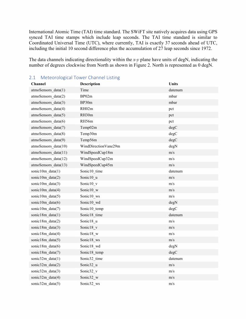
International Atomic Time (TAI) time standard. The SWiFT site natively acquires data using GPS

synced TAI time stamps which include leap seconds. The TAI time standard is similar to

Coordinated Universal Time (UTC), where currently, TAI is exactly 37 seconds ahead of UTC,

including the initial 10 second difference plus the accumulation of 27 leap seconds since 1972.

The data channels indicating directionality within the x-y plane have units of degN, indicating the

number of degrees clockwise from North as shown in Figure 2. North is represented as 0 degN.

2.1 Meteorological Tower Channel Listing

Channel Description Units

atmoSensors_data(1) Time datenum

atmoSensors_data(2) BP02m mbar

atmoSensors_data(3) BP30m mbar

atmoSensors_data(4) RH02m pct



atmoSensors_data(7) Temp02m degC



atmoSensors_data(10) WindDirectionVane29m degN

atmoSensors_data(11) WindSpeedCup18m m/s



sonic10m_data(1) Sonic10_time datenum

sonic10m_data(2) Sonic10_u m/s

sonic10m_data(3) Sonic10_v m/s

sonic10m_data(4) Sonic10_w m/s

sonic10m_data(5) Sonic10_ws m/s

sonic10m_data(6) Sonic10_wd degN

sonic10m_data(7) Sonic10_temp degC





























sonic_pos_data(1) Sonic10_position x(m), y(m), z(m)





atmoSensors_pos_data(1) WindDirectionVane29m_position x(m), y(m), z(m)

atmoSensors_pos_data(2) WindSpeedCup18m_position x(m), y(m), z(m)



atmoSensors_pos_data(5) BP_RH_Temp_02m_position x(m), y(m), z(m)

atmoSensors_pos_data(6) BP_RH_Temp_30m_position x(m), y(m), z(m)

atmoSensors_pos_data(7) RH_Temp_56m_position x(m), y(m), z(m)

atmoSensors_variables variable list corresponding to atmoSensors_data

stmoSensors_units unit list corresponding to atmoSensors_data

sonic_10m_variables variable list corresponding to sonic_10m_data

sonic_10m_units unit list corresponding to sonic_10m_data









sonic_pos_variables variable list corresponding to sonic_pos_data

sonic_pos_units unit list corresponding to sonic_pos_data

atmoSensors_pos_variables variable list corresponding to atmoSensors_pos_data

atmoSensors_pos_units unit list corresponding to atmoSensors_pos _data

2.2 Wind Turbine Channel Listing


data(1) Time datenum

data(2) NacWindSpeed m/s

data(3) NacWindDir deg

data(4) YawHeading deg

data(5) Azimuth deg

data(6) LSSTach1 rpm

data(7) HSSTach1_Smooth rpm

data(8) GenPwr kW

data(9) GenTq Nm

data(10) BldPitch1 deg

variables list of variables

units list of variable units

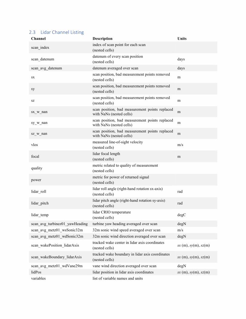
2.3 Lidar Channel Listing


scan_index index of scan point for each scan

(nested cells)

scan_datenum datenum of every scan position

(nested cells) days

scan_avg_datenum datenum averaged over scan days

sx scan position, bad measurement points removed

(nested cells) m

sy scan position, bad measurement points removed

(nested cells) m

sz scan position, bad measurement points removed

(nested cells) m

sx_w_nan scan position, bad measurement points replaced

with NaNs (nested cells) m

sy_w_nan scan position, bad measurement points replaced


sz_w_nan scan position, bad measurement points replaced


vlos measured line-of-sight velocity

(nested cells) m/s

focal lidar focal length

(nested cells) m

quality metric related to quality of measurement

(nested cells)

power metric for power of returned signal

(nested cells)

lidar_roll lidar roll angle (right-hand rotation sx-axis)

(nested cells) rad

lidar_pitch lidar pitch angle (right-hand rotation sy-axis)

(nested cells) rad

lidar_temp lidar CRIO temperature

(nested cells) degC

scan_avg_turbinez01_yawHeading turbine yaw heading averaged over scan degN

scan_avg_metz01_wsSonic32m 32m sonic wind speed averaged over scan m/s

scan_avg_metz01_wdSonic32m 32m sonic wind direction averaged over scan degN

scan_wakePosition_lidarAxis tracked wake center in lidar axis coordinates

(nested cells) sx (m), sy(m), sz(m)

scan_wakeBoundary_lidarAxis tracked wake boundary in lidar axis coordinates

(nested cells) sx (m), sy(m), sz(m)

scan_avg_metz01_wdVane29m vane wind direction averaged over scan degN

lidPos lidar position in lidar axis coordinates sx (m), sy(m), sz(m)

variables list of variable names and units

3 National Instruments CompactRIO The National Instruments CompactRIO (CRIO) provides the platform for turbine control and data

acquisition at the SWiFT site. Data from the meteorological towers and turbines consists of both

digital RS-422 serial communications and analog voltage signals and therefore different interface

modules are connected to the CRIO. Digital signals are acquired by NI 9871 serial interface

modules. Turbine analog signals are acquired by NI 9205, which have a - 10 – 10 V full-scale

range with 16-bit resolution, while met tower analog signals are acquired by NI 9239, which have

- 10 – 10 V full-scale range with 24-bit resolution. The SWiFT site time synchronization is

provided by Global Positioning System (GPS) time stamps in the International Atomic Time (TAI)

standard.

4 Meteorological Towers

4.1 Sonic Anemometers

Five SATI Series ‘A’ style probe ultrasonic anemometers from ATI Technologies Inc. are located

at 10 m, 18 m, 32 m, 45 m, and 58 m above the ground on the METa1 and METb1 towers. The

anemometers sample data at 100 Hz and measure u, v, and w velocity components of the wind, as

well as the temperature, T, based on the time of flight of a sound signal and the speed of sound

calculation. In the provided data, the u vector points North, v points West, and w points up, as

shown in Figure 2, which provides the SWiFT site coordinate system. The anemometers output

data using the RS-422 serial protocol. Occasionally this signal has a spurious spike. The provided

data are quality controlled to remove spikes using the median absolute deviation. The median

window has a length 3,000 data points (30 seconds). Data more than four standard deviations away

from the median are removed, and appear as NaN. Early sonic anemometer data sets (prior to

January 20th, 2017) used time stamps supplied by the CRIO. Large time drifts on the order of

minutes relative to the GPS synced data were observed with this method and corrected for using u

and v velocity component data sampled at 20 Hz with GPS time stamps. Since January 20th 2017,

all sonic anemometer data are sampled at 100 Hz with GPS time stamps. Thus, all of the Quality

Assured and Quality Controlled (QA/QC) data provided has GPS-synced time stamps. In addition

to the time stamp correction, the u, v, and w velocity components have been transformed from

their raw orientation to the u, v, and w coordinate system of the SWiFT site. The roll and pitch

rotation correction was determined by minimizing the standard deviation of the vertical velocity

component as a function of wind direction for 60 minute averages over 1.5 months [2]. Data bins

acquired with large wind direction changes or too high/low turbulence intensity were not included

in the analysis. The yaw angle correction was calculated through comparisons with the calibrated

wind vane and verified through total station theodolite (TST) measurements of the boom arms.

Note that even though the sonic anemometers sample data at 100 Hz, frequencies above 20 Hz are

likely contaminated by met tower dynamics.

4.2 Cup Anemometers

Three Wind Sensor First Class Advanced cup anemometers from Thies Clima are located 18 m,

31.5 m, and 45 m above the ground. The analog sensors output a frequency that is proportional to

wind speed, 21.8 Hz/m/s. The cup anemometers are located approximately at the rotor bottom,

hub, and rotor top heights. Data are sampled at 20 Hz. Occasionally this signal has a spurious

spike. The provided data are quality controlled to remove spikes using the median absolute

deviation. The median window has a length 3,000 data points (30 seconds). Data more than four

standard deviations away from the median are removed, and appear as NaN.

4.3 Wind Vane

One Thies Clima Wind Direction Sensor First Class measures wind direction at the hub height,

29.5 m. It outputs an analog voltage that is proportional to compass wind direction. Data are

sampled at 20 Hz. The wind vane was calibrated to the SWiFT coordinate system by aligning the

wind vane to two distant land marks with measured GPS positions. Note that presently there is a

consistent, small nonlinearity when comparing the wind vane to the each of the sonic anemometer

measured wind directions. This behavior was observed during the QA/QC process discussed in the

sonic anemometer section. The nonlinearity was removed in calculating the sonic anemometer

orientation by assuming a slope of one in the comparison and assuming the difference between a

linear and the nonlinear calibration should average to zero. The nonlinear response has not yet

been removed in the provided data, but a table-top calibration will be applied in the near future.

4.4 Barometric Pressure

Two Met One Instruments Inc. 092 Barometric Pressure sensors output a 0 – 5 V signal. The

device was configured for high altitude application with a full-scale range of 800 – 1000 mbar.

Pressures sensors are located at 2 m and 27.5 m above the ground. Data are sampled at 20 Hz.

4.5 Relative Humidity

Met One Instruments Inc. provides the 593 Relative Humidity sensors located at tower heights

2 m, 27.5 m, and 56.5 m. These analog instruments output a 0 – 1 V signal for a 0 – 100% humidity

full-scale range. Data are sampled at 20 Hz. The Relative Humidity acquired at a height of 56.5 m

has a large amount a noise, likely due to a grounding issue that has not yet been resolved.

4.6 Temperature

Met One Instruments Inc. provides the 9250 temperature sensors located at tower heights 2 m,

27.5 m, and 56.5 m. These analog instruments output a 0 – 1 V signal for a -30 °C – 50 °C full-

scale range. Data are sampled at 20 Hz. The temperature acquired at a height of 56.5 m has a large

amount a noise, likely due to a grounding issue that has not yet been resolved.

5 Turbine Sensors

5.1 Nacelle Wind Sensor

The FT702LT Version 22 wind sensor, made by FT Technologies Ltd, uses acoustic resonance to

measure wind speed and wind direction. This sensor only measures a lateral velocity parallel to

the ground and gives no vertical component of wind speed. Data are sampled at 50 Hz, but only

updated at 1 measurement per second. The provided data are quality controlled to remove spikes

using the median absolute deviation. The median window has a length 3,000 data points (30

seconds). Data more than four standard deviations away from the median are removed, and appear

as NaN.

5.2 Yaw Heading

US Digital provides the HD25A absolute, optical, rotary encoder. The default 3600

counts/revolution is used to keep track of the nacelle yaw angle relative to the cardinal direction

coordinate system. The encoder provides a resolution of 1 pulse per 0.01 degrees with an

additional gear ratio providing a yaw heading resolution of 0.001 degrees. Data are sampled at

50 Hz. The absolute yaw position of the yaw encoder was calibrated using TST measurements of

bolts along both sides of the nacelle bed plate. The bolt position measurements were least-squares

fit with planes corresponding to the sides of the bed plate. The nacelle centerline was calculated

as the average between the two planes. The nacelle centerline was transformed to the SWiFT

coordinate system using site surveying markers that indicate true North. The TST calibration of

the yaw encoder was verified with a plumb bob used to align the low-speed shaft with a surveying

marker.

5.3 Azimuth Angle

The MIR 3000F HDmag Flex sensing head and magnetic belt, made by Gaumer Group, function

as an incremental encoder with magnetic sensing. The magnetic belt is wrapped around the

circumference of the low speed shaft, and the sensing head measures the rotational velocity of the

shaft and the absolute azimuthal angle. Data are sampled at 50 Hz. The azimuth angle has not yet

been calibrated to the zero angle position of the rotor.

5.4 Low Speed Shaft Tachometer

Carlo Gavazzi provides the DU10E inductive proximity sensor. The sensor provides a digital

output by measuring the passing of 14 equally spaced flag-shaped sensor targets on the low-speed

shaft. The angular velocity is calculated from the time between rising edges per 25.71 degrees.

Data are sampled at 50 Hz.

5.5 High Speed Shaft Tachometer – Smoothed

Telemecanique provides the XS1M18PA370 inductive proximity sensor. The sensor measures

3 equally spaced lobes on the high speed shaft that pass the sensor providing a digital output. The

angular velocity is calculated from the time per 360 degrees and updated at every 120 degrees. A

moving average with a 24 ms window is used to smooth the measurement prior to logging the data

at 50 Hz.

5.6 Generator Power and Generator Torque

Power and torque are reported by the ABB ACS800-17 Variable Frequency Drive. The power and

torque values are updated with a resolution of 0.3 kW and 0.16 Nm, respectively, and the data are

logged at 50 Hz. A 100 ms filter is applied to the generator torque data before logging

5.7 Blade Pitch

The blade pitch is controlled by the traverse tube extension through a pitch linkage. The kinematics

have been modeled in detail and Figure 5 shows the relationship between the measured traverse

tube extension in meters, and the blade pitch in degrees. A blade pitch of 1 degree is used during

Region 2 and 2.5 of power generation, and the blade feathers towards 88 degrees in Region III and

shutdown to shed load.

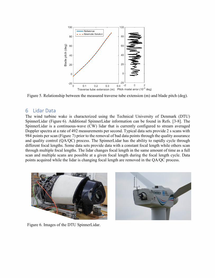
Figure 5. Relationship between the measured traverse tube extension (m) and blade pitch (deg).

6 Lidar Data The wind turbine wake is characterized using the Technical University of Denmark (DTU)

SpinnerLidar (Figure 6). Additional SpinnerLidar information can be found in Refs. [3-8]. The

SpinnerLidar is a continuous-wave (CW) lidar that is currently configured to stream averaged

Doppler spectra at a rate of 492 measurements per second. Typical data sets provide 2 s scans with

984 points per scan (Figure 7) prior to the removal of bad data points through the quality assurance

and quality control (QA/QC) process. The SpinnerLidar has the ability to rapidly cycle through

different focal lengths. Some data sets provide data with a constant focal length while others scan

through multiple focal lengths. The lidar changes focal length in the same amount of time as a full

scan and multiple scans are possible at a given focal length during the focal length cycle. Data

points acquired while the lidar is changing focal length are removed in the QA/QC process.

Figure 6. Images of the DTU SpinnerLidar.

Figure 7. Calibrated DTU SpinnerLidar scan points in normalized lidar coordinates and lidar

probe volume weighting function vs focal length.

The SpinnerLidar calculates the line-of-sight velocity from the returned Doppler spectra by

calculating the centroid of frequencies observed within the probe volume above a noise threshold.

Future documentation will outline the lidar QA/QC process in greater detail, but briefly, the

method removes data points that have a low level of laser signal return relative to the noise

threshold as well as points contaminated with laser signal returns from stationary objects. The

removal of points with laser returns from stationary objects primarily removes points contaminated

with ground returns and boresight returns. The boresight returns are due to laser reflections from

the outer window and appear at the center of the scan pattern. Sometimes this removal includes

points due to returns from the met towers and neighboring SWiFT wind turbines.

The lidar measurement location is aligned and calibrated using the method provided in Ref. [9].

The measurements are transformed into the coordinate system in Figure 2 (referred to as the lidar

coordinate system), where the sx direction is aligned with the centerline of the nacelle axial

direction, sz is vertical, and sy is oriented to create a right-handed coordinate system. The location

of the measurements in the lidar coordinate system are scaled from an initial normalized frame

(which was calibrated in Ref. [9]) using the average focal length over the scan. The actual focal

length at each measurement point can fluctuate as high as ± 2 m. This fluctuation is relatively small

when compared to the probe volume length of the lidar (Figure 7) [10, 11]. The orientation and

position of the lidar relative to the ground and nacelle was determined using total station theodolite

(TST) measurements [9]. The lidar roll and pitch angles (Figure 8) are measured by a calibrated

3-axis accelerometer [9], and applied to the data to create the lidar coordinate system (sx, sy, sz).

The origin of the coordinate system is centered along the nacelle yaw rotation axis and located at

the base of the turbine foundation. The vertical coordinate in the lidar coordinate frame matches

the vertical coordinate of the SWiFT site coordinate frame, and the SWiFT site x-y plane matches

the lidar sx-sy plane. Thus, the only difference between the coordinate systems is due to the yaw

-0.5-0.4-0.3-0.2-0.100.10.20.30.40.5

ny

-0.5

-0.4

-0.3

-0.2

-0.1

0

0.1

0.2

0.3

0.4

0.5n

z

0 50 100 150 200

sx (m)

0

0.1

0.2

0.3

0.4

0.5

pro

be v

ol w

eig

hting function

f = 1D, fwhm = 1.36 (m)

f = 2D, fwhm = 5.42 (m)

f = 2.5D, fwhm = 8.44 (m)

f = 3D, fwhm = 12.11 (m)

f = 4D, fwhm = 21.32 (m)

f = 5D, fwhm = 32.90 (m)

heading of the turbine. The lidar coordinate system can be transformed into the SWiFT site

coordinate system by applying a rotation around the sz axis with a magnitude corresponding to the

yaw heading. The lidar coordinate system is implemented as a balance between ease of data use

and limited levels of initial processing for the data user. Users of the data should be able to easily

transform the lidar coordinate system to the cardinal direction coordinate system or wind direction

coordinate system as needed.

Figure 8. Lidar roll and pitch orientation schematic.

The time stamps on the lidar data are provided as datenum units. The SWiFT site natively acquires

data using GPS synced TAI time stamps, while the lidar uses GPS synced Coordinated Universal

Time (UTC) time stamps. The lidar time stamps have been adjusted to account for the 10 s base

and leap seconds difference between the time standards and finally, to the supplied datenum units.

Thus, the lidar data and SWiFT site data are highly synchronized.

The lidar data files are structured as variables with nested cell data types. Each file contains

approximately 10 minutes of scans. The nested cell data types are needed because each scan can

have a different number of points. Many of the provided lidar data channels are not required. The

data has already been processed for QA/QC and the lidar coordinates have been transformed, so

the quality, power, pitch, and roll channels are not necessary for the typical data user. The lidar

data also contains a number of relevant met and turbine channels averaged over each scan. Figure 9

displays sample images from the lidar data at 1 – 5 D (D = 27m) downstream of the turbine. The

irregular scan pattern was interpolated to a regular grid using a smoothing surface fit, while the

wake position was calculated using an image processing object detection method of the velocity

wake deficit. The calculated wake center and boundary are provided in the data files but the

regularized interpolated velocity points are not.

x

z

y

rollpitch

yaw

Figure 9. Example lidar measurements at 1 – 5 D.

7 References 1. Berg, J., Bryant, J., LeBlanc, B., Maniaci, D. C., Naughton, B., Paquette, J. A., Resor, B.

R., White, J., and Kroeker, D. "Scaled Wind Farm Technology Facility Overview," 32nd

ASME Wind Energy Symposium. American Institute of Aeronautics and Astronautics,

2014.

2. Kelley, C. L., and Ennis, B. L. "SWiFT Site Atmospheric Characterization," SAND-2016-

2016. Sandia National Laboratories, 2016.

3. Sjöholm, M., Pedersen, A. T., Angelou, N., Abari, F. F., Mikkelsen, T. K., Harris, M.,

Slinger, C., and Kapp, S. "Full two-dimensional rotor plane inflow measurements by a

spinner-integrated wind lidar," European Wind Energy Association Conference. 2013.

4. Mikkelsen, T., Angelou, N., Hansen, K., Sjöholm, M., Harris, M., Slinger, C., Hadley, P.,

Scullion, R., Ellis, G., and Vives, G. "A spinner-integrated wind lidar for enhanced wind

turbine control," Wind Energy Vol. 16, No. 4, 2013, pp. 625-643.

doi: 10.1002/we.1564

5. Machefaux, E., Larsen, G. C., Troldborg, N., Hansen, K. S., Angelou, N., Mikkelsen, T.,

and Mann, J. "Investigation of wake interaction using full-scale lidar measurements and

large eddy simulation," Wind Energy Vol. 19, No. 8, 2016, pp. 1535-1551.

doi: 10.1002/we.1936

6. Angelou, N., and Sjöholm, M. "UniTTe WP3/MC1: Measuring the inflow towards a

Nordtank 500kW turbine using three short-range WindScanners and one SpinnerLidar."

DTU Wind Energy, 2015.

7. Churchfield, M., Wang, Q., Scholbrock, A., Herges, T., Mikkelsen, T., and Sjöholm, M.

"Using High-Fidelity Computational Fluid Dynamics to Help Design a Wind Turbine

Wake Measurement Experiment," Journal of Physics: Conference Series Vol. 753, No. 3,

2016, p. 032009.

8. Herges, T. G., Maniaci, D. C., Naughton, B. T., Mikkelsen, T., and Sjöholm, M. "High

resolution wind turbine wake measurements with a scanning lidar," EWEA Wake

Conference, To Be Published. 2017.

9. Herges, T. G., Maniaci, D. C., Naughton, B., Hansen, K., Sjöholm, M., Angelou, N., and

Mikkelsen, T. "Scanning Lidar Spatial Calibration and Alignment Method for Wind

Turbine Wake Characterization," 35th Wind Energy Symposium. American Institute of

Aeronautics and Astronautics, 2017.

10. Angelou, N., Mann, J., Sjöholm, M., and Courtney, M. "Direct measurement of the spectral

transfer function of a laser based anemometer," Review of Scientific Instruments Vol. 83,

No. 3, 2012, p. 033111.

doi: 10.1063/1.3697728

11. Horváth, Z. L., and Bor, Z. "Focusing of truncated Gaussian beams," Optics

Communications Vol. 222, No. 1–6, 2003, pp. 51-68.

doi: http://dx.doi.org/10.1016/S0030-4018(03)01562-1

swift wake steering instrumentation and data processing · swift wake steering instrumentation and...

Documents