Syllabus for Math 2250-004 Di↵erential Equations and Linear Algebra

Spring 2017

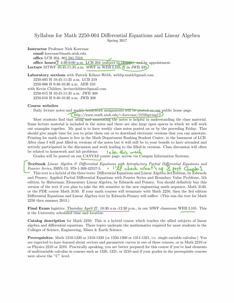
Instructor Professor Nick Korevaaremail korevaar@math.utah.eduo�ce LCB 204, 801.581.7318o�ce hours T 4:30-6:00 p.m. LCB 204 (subject to change), and by appointment.

Lecture MTWF 10:45-11:35 a.m. MWF in WEB L105, T in JWB 335

Laboratory sections with Patrick Kilmer-Webb, webbp.math@gmail.com2250-005 H 10:45-11:35 a.m. LCB 2192250-006 H 9:40-10:30 a.m. AEB 310

with Kevin Childers, kevinrchilders@gmail.com2250-015 H 10:45-11:35 a.m. JWB 3082250-016 H 9:40-10:30 a.m. JWB 308

Course websitesDaily lecture notes and weekly homework assignments will be posted on our public home page.

http://www.math.utah.edu/⇠korevaar/2250spring17

Most students find that using and annotating the notes is helpful in understanding the class material.Some lecture material is included in the notes and there are also large open spaces in which we will workout examples together. My goal is to have weekly class notes posted on or by the preceding Friday. Thisshould give ample time for you to print them out or to download electronic versions that you can annotate.Printing for math classes is free in the Math Department Rushing Student Center, in the basement of LCB.After class I will post filled-in versions of the notes but it will still be to your benefit to have attended andactively participated in the discussion and work leading to the filled-in versions. Class discussion will oftenbe related to homework and lab problems.

Grades will be posted on our CANVAS course page; access via Campus Information Systems.

Textbook Linear Algebra & Di↵erential Equations with Introductory Partial Di↵erential Equations and

Fourier Series, ISBN-13: 978-1-269-42557-5.This text is a hybrid of the three texts: Di↵erential Equations and Linear Algebra 3rd Edition, by Edwards

and Penney; Applied Partial Di↵erential Equations with Fourier Series and Boundary Value Problems, 5thedition, by Haberman; Elementary Linear Algebra, by Edwards and Penney. You should definitely buy thisversion of the text if you plan to take the 4th semester in the new engineering math sequence, Math 3140,or the PDE course Math 3150. If your math courses will terminate with Math 2250, then the 3rd editionDi↵erential Equations and Linear Algebra text by Edwards-Penney will su�ce. (This was the text for Math2250 thru summer 2013.)

Final Exam logistics: Thursday April 27, 10:30 a.m.-12:30 p.m., in our MWF classroom WEB L105. Thisis the University scheduled time and location.

Catalog description for Math 2250: This is a hybrid course which teaches the allied subjects of linearalgebra and di↵erential equations. These topics underpin the mathematics required for most students in theColleges of Science, Engineering, Mines & Earth Science.

Prerequisites: Math 1210-1220 or 1310-1320 (or 1250-1260 or 1311-1321, i.e. single-variable calculus.) Youare expected to have learned about vectors and parametric curves in one of these courses, or in Math 2210 oror Physics 2210 or 3210. Practically speaking, you are better prepared for this course if you’ve had elementsof multivariable calculus in courses such as 1320, 1321, or 2210 and if your grades in the prerequisite courseswere above the ”C” level.

1

Learning Objectives for 2250

The goal of Math 2250 is to master the basic tools and problem solving techniques important in di↵erentialequations and linear algebra. These basic tools and problem solving skills are described below.

The essential topicsBe able to model dynamical systems that arise in science and engineering, by using general principles

to derive the governing di↵erential equations or systems of di↵erential equations. These principles includelinearization, compartmental analysis, Newton’s laws, conservation of energy and Kircho↵’s law.

Learn solution techniques for first order separable and linear di↵erential equations. Solve initial valueproblems in these cases, with applications to problems in science and engineering. Understand how toapproximate solutions even when exact formulas do not exist. Visualize solution graphs and numericalapproximations to initial value problems via slope fields. Understand phase diagram analysis for autonomousfirst order di↵erential equations.

Become fluent in matrix algebra techniques, in order to be able to compute the solution space to linearsystems and understand its structure; by hand for small problems and with technology for large problems.

Be able to use the basic concepts of linear algebra such as linear combinations, span, independence, basisand dimension, to understand the solution space to linear equations, linear di↵erential equations, and linearsystems of di↵erential equations.

Understand the natural initial value problems for first order systems of di↵erential equations, and howthey encompass the natural initial value problems for higher order di↵erential equations and general systemsof di↵erential equations.

Learn how to solve constant coe�cient linear di↵erential equations via superposition, particular solutions,and homogeneous solutions found via characteristic equation analysis. Apply these techniques to understandthe solutions to the basic unforced and forced mechanical and electrical oscillation problems.

Learn how to use Laplace transform techniques to solve linear di↵erential equations, with an emphasison the initial value problems of mechanical systems, electrical circuits, and related problems.

Be able to find eigenvalues and eigenvectors for square matrices. Apply these matrix algebra concepts tofind the general solution space to first and second order constant coe�cient homogeneous linear systems ofdi↵erential equations, especially those arising from compartmental analysis and mechanical systems.

Understand and be able to use linearization as a technique to understand the behavior of nonlineardynamical systems near equilibrium solutions. Apply these techniques to non-linear mechanical oscillationproblems. (Additional material, subject to time availability: Apply linearization to autonomous systemsof two first order di↵erential equations, including interacting populations. Relate the phase portraits ofnon-linear systems near equilibria to the linearized data, in particular to understand stability.)

Develop your ability to communicate modeling and mathematical explanations and solutions, using tech-nology and software such as Maple, Matlab or internet-based tools as appropriate.Problem solving fluency

Students will be able to read and understand problem descriptions, then be able to formulate equationsmodeling the problem usually by applying geometric or physical principles. Solving a problem often requiresspecific solution methods listed above. Students will be able to select the appropriate operations, executethem accurately, and interpret the results using numerical and graphical computational aids.

Students will also gain experience with problem solving in groups. Students should be able to e↵ectivelytransform problem objectives into appropriate problem solving methods through collaborative discussion.Students will also learn how to articulate questions e↵ectively with both the instructor and TA, and be ableto e↵ectively convey how problem solutions meet the problem objectives.

3

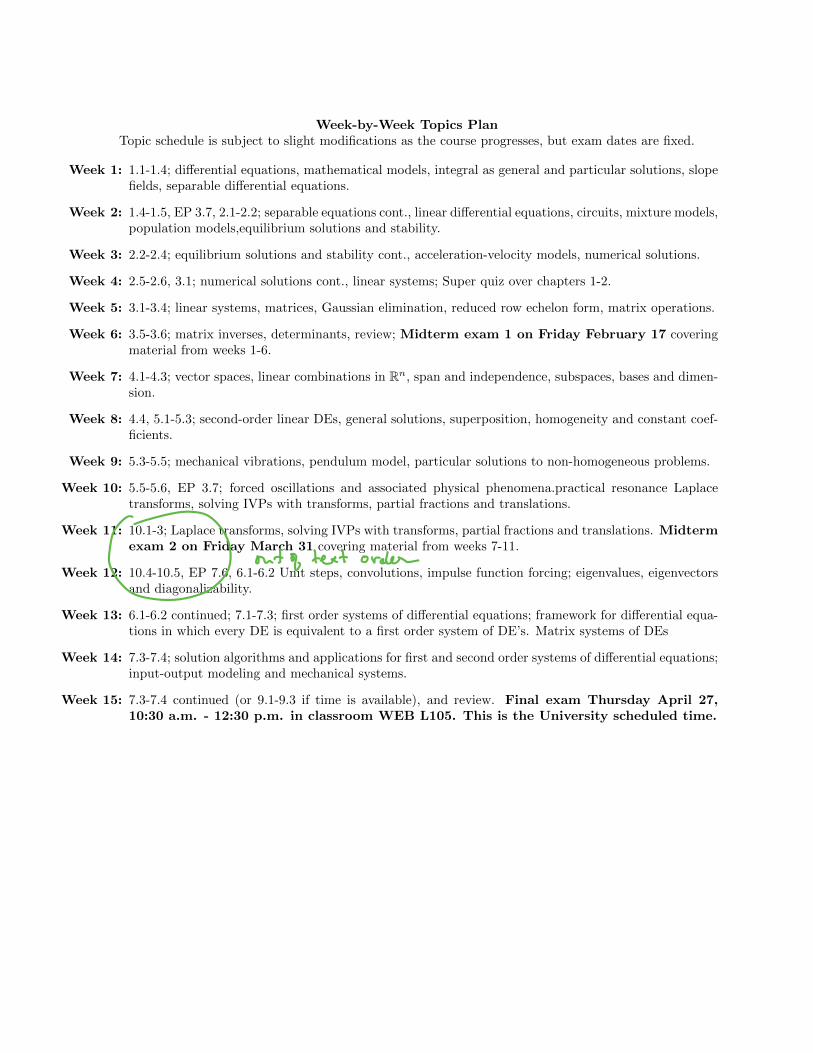
Week-by-Week Topics PlanTopic schedule is subject to slight modifications as the course progresses, but exam dates are fixed.

Week 1: 1.1-1.4; di↵erential equations, mathematical models, integral as general and particular solutions, slopefields, separable di↵erential equations.

Week 2: 1.4-1.5, EP 3.7, 2.1-2.2; separable equations cont., linear di↵erential equations, circuits, mixture models,population models,equilibrium solutions and stability.

Week 3: 2.2-2.4; equilibrium solutions and stability cont., acceleration-velocity models, numerical solutions.

Week 4: 2.5-2.6, 3.1; numerical solutions cont., linear systems; Super quiz over chapters 1-2.

Week 5: 3.1-3.4; linear systems, matrices, Gaussian elimination, reduced row echelon form, matrix operations.

Week 6: 3.5-3.6; matrix inverses, determinants, review; Midterm exam 1 on Friday February 17 coveringmaterial from weeks 1-6.

Week 7: 4.1-4.3; vector spaces, linear combinations in Rn, span and independence, subspaces, bases and dimen-sion.

Week 8: 4.4, 5.1-5.3; second-order linear DEs, general solutions, superposition, homogeneity and constant coef-ficients.

Week 9: 5.3-5.5; mechanical vibrations, pendulum model, particular solutions to non-homogeneous problems.

Week 10: 5.5-5.6, EP 3.7; forced oscillations and associated physical phenomena.practical resonance Laplacetransforms, solving IVPs with transforms, partial fractions and translations.

Week 11: 10.1-3; Laplace transforms, solving IVPs with transforms, partial fractions and translations. Midtermexam 2 on Friday March 31 covering material from weeks 7-11.

Week 12: 10.4-10.5, EP 7.6, 6.1-6.2 Unit steps, convolutions, impulse function forcing; eigenvalues, eigenvectorsand diagonalizability.

Week 13: 6.1-6.2 continued; 7.1-7.3; first order systems of di↵erential equations; framework for di↵erential equa-tions in which every DE is equivalent to a first order system of DE’s. Matrix systems of DEs

Week 14: 7.3-7.4; solution algorithms and applications for first and second order systems of di↵erential equations;input-output modeling and mechanical systems.

Week 15: 7.3-7.4 continued (or 9.1-9.3 if time is available), and review. Final exam Thursday April 27,10:30 a.m. - 12:30 p.m. in classroom WEB L105. This is the University scheduled time.

4

Math 2250-004 Week 1 notesWe will not necessarily finish the material from a given day's notes on that day. We may also add or subtract some material as the week progresses, but these notes represent an in-depth outline of what we will cover. These notes are for sections 1.1-1.3, and part of 1.4.

Monday January 9

Go over course information on syllabus and course homepage:

http://www.math.utah.edu/~korevaar/2250spring17

Note that there is a quiz this Wednesday on the material we cover today and tomorrow, and that your first lab meeting is this Thursday. Your first homework assignment will be due next Wednesday, January 17.

Then, let's begin! What is an nth order differential equation (DE)?

any equation involving a function y = y x and its derivatives, for which the highest derivative appearing in the equation is the nth one, y n x ; i.e. any equation which can be written as

F x, y x , y x , y x ,...y n x = 0.

Exercise 1: Which of the following are differential equations? For each DE determine the order.a) For y = y x , y x 2 sin y x = 0 b) For x = x t , x t = 3 x t 10 x t .c) For x = x t , x = 3 x 10 x .d) For z = z r , z r 4 z r .e) For y = y x , y = y2 .

A solution function y x to the differential equation F x, y, y , y , y n = 0 defined on some interval I is any function y x which makes the differential equation a true equality for all x in I.

A solution function y x to a first order differential equation F x, y, y = 0 on the interval I which also satisifies y x0 = y0 for a specified x0 I and y0 is called a solution to the initial value problem (IVP)

F x, y, y = 0

y x0 = y0.

Exercise 2: Consider the differential equation dydx

= y2 from (1e).

2a) Show that functions y x =1

C x solve the DE (on any interval not containing the constant C).

2b) Find the appropriate value of C to solve the initial value problemy = y2

y 1 = 2 .

2c) What is the largest interval on which your solution to (b) is defined as a differentiable function? Why?

2d) Do you expect that there are any other solutions to the IVP in 2b? Hint: The graph of the IVP solution function we found is superimposed onto a "slope field" below: The line segments at points x, y have values y2, because solutions graphs to the differential equation

y = y2 will have slopes given by the derivatives of the solutions y x . This might give you some intuition about whether you expect more than one solution to the IVP.