symbolic context-sensitive pointer analysisjzhu/publications/calman_master.pdf · symbolic...
TRANSCRIPT
SYMBOLIC CONTEXT-SENSITIVE POINTER ANALYSIS
by
Silvian Calman
A thesis submitted in conformity with the requirementsfor the degree of Masters of Science
Graduate Department of Electrical and Computer EngineeringUniversity of Toronto
Copyright c© 2005 by Silvian Calman
Abstract
Symbolic Context-Sensitive Pointer Analysis
Silvian Calman
Masters of Science
Graduate Department of Electrical and Computer Engineering
University of Toronto
2005
Pointer analysis is a critical problem in optimizing compiler, parallelizing compiler, software
engineering and most recently, hardware synthesis. While recent efforts have suggested sym-
bolic method, which uses Bryant’s Binary Decision Diagram as an alternative to capture the
point-to relation, no speed advantage has been demonstrated for context-insensitive analysis,
and results for context-sensitive analysis are only preliminary.
We refine the concept of symbolic transfer function proposed earlier and establish a com-
mon framework for both context-insensitive and context-sensitive pointer analysis. With this
framework, the transfer function of a procedure can abstract away the impact of its callers and
callees, and represent its point-to information completely, compactly and canonically. In ad-
dition, we propose a symbolic representation of the invocation graph, which can otherwise be
exponentially large. In contrast to the classical frameworks where context-sensitive point-to
information of a procedure has to be obtained by the application of its transfer function expo-
nentially many times, our method can obtain point-to information of all contexts in a single
application. Our experimental evaluation on a wide range of C benchmarks indicates that our
context-sensitive pointer analysis can be made almost as fast as its context-insensitive counter-
part.
ii

Acknowledgements
I would like to thank my advisor, Jianwen Zhu, for always keeping the door open, and his
patience; he has been a perfect role model for what a researcher should be, and I learned a lot
from him. Besides his many suggestions, he motivated me by example, and forced me to think.
I would also like to thank our research group, and in particular, Linda, Rami, and Dennis
who were always there to talk or just give advice. In addition, I thank the people I shared the
lab with over the years, and in particular, Chris, Christine, and Gerald; I enjoyed our many
conversations.
Throughout my M.A.Sc I took courses, thanks to Michael Voss, Derek Corneil, Tarek Ab-
delrahman, Greg Steffan, and my advisor, Jianwen Zhu for teaching them.
This work was made possible by the support from NSERC and OGS.
Lastly, I would like to thank my family for their support, love, and encouragement. They
always wanted what was best for me.
iii
Table of Contents
Abstract ii
Acknowledgements iii
List of Figures vi
List of Tables vii
List of Acronyms viii
1 Introduction 1
1.1 Motivation . . . . . . . . . . . . . . . . . . . . . . . . . . . . . . . . . . . . . 1
1.2 Contributions . . . . . . . . . . . . . . . . . . . . . . . . . . . . . . . . . . . 5
1.3 Thesis Organization . . . . . . . . . . . . . . . . . . . . . . . . . . . . . . . . 6
2 Related Work 7
3 Symbolic Program Modeling 13
3.1 Preliminary . . . . . . . . . . . . . . . . . . . . . . . . . . . . . . . . . . . . 13
3.2 Symbolic Program State . . . . . . . . . . . . . . . . . . . . . . . . . . . . . 16
3.3 Symbolic Transfer Function . . . . . . . . . . . . . . . . . . . . . . . . . . . 19
3.4 Binary Decision Diagrams . . . . . . . . . . . . . . . . . . . . . . . . . . . . 21
3.5 Recurrence Equations . . . . . . . . . . . . . . . . . . . . . . . . . . . . . . . 25
iv

3.6 Symbolic State Query . . . . . . . . . . . . . . . . . . . . . . . . . . . . . . . 27
3.7 Symbolic Transfer Function Application . . . . . . . . . . . . . . . . . . . . . 28
4 Symbolic Context-Sensitive Analysis 31
4.1 Invocation Graph . . . . . . . . . . . . . . . . . . . . . . . . . . . . . . . . . 31
4.2 Acyclic Call Graph Reduction . . . . . . . . . . . . . . . . . . . . . . . . . . 34
4.3 Deriving Symbolic Edge Relations . . . . . . . . . . . . . . . . . . . . . . . . 37
4.4 Context-Sensitive Analysis . . . . . . . . . . . . . . . . . . . . . . . . . . . . 41
5 Experimental Results 43
5.1 Space Efficiency . . . . . . . . . . . . . . . . . . . . . . . . . . . . . . . . . 46
5.2 Runtime Efficiency . . . . . . . . . . . . . . . . . . . . . . . . . . . . . . . . 47
5.3 Precision . . . . . . . . . . . . . . . . . . . . . . . . . . . . . . . . . . . . . 51
5.4 Impact of Caching . . . . . . . . . . . . . . . . . . . . . . . . . . . . . . . . . 52
5.5 Impact of Lazy Garbage Collection . . . . . . . . . . . . . . . . . . . . . . . . 53
5.6 Impact of Variable Reordering . . . . . . . . . . . . . . . . . . . . . . . . . . 55
6 Conclusion 57
Appendix 65
A Solution Process Illustration . . . . . . . . . . . . . . . . . . . . . . . . . . . 65
v
List of Figures
2.1 Point-to graph generated using Steensgaard’s and Andersen’s algorithms for
the source code shown in Figure 2.1 (a) . . . . . . . . . . . . . . . . . . . . . 8
3.1 C source code . . . . . . . . . . . . . . . . . . . . . . . . . . . . . . . . . . . 17
3.2 Program state on the completion of Figure 3.1. . . . . . . . . . . . . . . . . . . 18
3.3 Transfer Function, A walk-through example. . . . . . . . . . . . . . . . . . . . 22
3.4 Transfer functions in BDD. . . . . . . . . . . . . . . . . . . . . . . . . . . . . 24
4.1 A Call Graph and Invocation Graph . . . . . . . . . . . . . . . . . . . . . . . 32
4.2 Deriving Invocation graph by processing SCCs . . . . . . . . . . . . . . . . . 37
4.3 Construction of helper symbolic relations. . . . . . . . . . . . . . . . . . . . . 40
5.1 Memory usage versus context count. . . . . . . . . . . . . . . . . . . . . . . . 47
5.2 Algorithm runtime versus context count. . . . . . . . . . . . . . . . . . . . . . 51
5.3 Precision result. . . . . . . . . . . . . . . . . . . . . . . . . . . . . . . . . . . 52
5.4 Cache hit rate. . . . . . . . . . . . . . . . . . . . . . . . . . . . . . . . . . . . 54
5.5 Time spent on garbage collection. . . . . . . . . . . . . . . . . . . . . . . . . 55
5.6 Variable Reordering . . . . . . . . . . . . . . . . . . . . . . . . . . . . . . . . 56
vi
List of Tables
3.1 Minterm map for program variables . . . . . . . . . . . . . . . . . . . . . . . 19
3.2 Transfer Function parameters minterm mapping . . . . . . . . . . . . . . . . . 21
3.3 Other Finals minterm mapping . . . . . . . . . . . . . . . . . . . . . . . . . . 22
5.1 Benchmark characteristics. . . . . . . . . . . . . . . . . . . . . . . . . . . . . 44
5.2 Boolean variable sets and their order . . . . . . . . . . . . . . . . . . . . . . . 45
5.3 Analysis runtime and space usage results for Mediabench benchmarks. . . . . . 48
5.3 Analysis runtime and space usage result for SPEC2K benchmarks. . . . . . . . 49
5.3 Analysis runtime and space usage result for prolangs benchmarks. . . . . . . . 50
vii

List of Acronyms
FI Flow-Insensitive
FS Flow-Sensitive
CI Context-Insensitive
CS Context-Sensitive
FICS Flow-Insensitive Context-Sensitive
FSCS Flow-Sensitive Context-Sensitive
FICI Flow-Insensitive Context-Insensitive
FSCI Flow-Sensitive Context-Insensitive
ROBDD Reduced Ordered Binary Decision Diagram
BDD Binary Decision Diagram (same as ROBDD)
SCC Strongly Connected Component
PTF Partial Transfer Function
LOC Line of Code
KLOC Thousand Line of Code
MLOC Million Line of Code
IR Intermediate Representation
viii
Chapter 1
Introduction
1.1 Motivation
Memory spaces are allocated for different program variables to hold their value. The address of
a program variable indicates the location of the value within a linear address space. A pointer
is a program variable whose value may contain the address of another program variable, in
which case the pointer is said to point to the program variable. A pointer can be dereferenced
if the value of the program variable it points to is retrieved.
By pointer dereference, a program can read and write a program variable indirectly. For
example, if program variable g points to program variable x, then we can read x by reading
the dereference of g. In addition, if we write a value to the dereference of g, the value will be
written at the address of x, and hence, we assign this value to x indirectly. Reading and writing
program variables indirectly is particularly useful when the variables are allocated on the heap.
These concepts are used to implement abstract data structures such as lists, hash tables, vectors,
graphs, and trees. The pointer can also be passed as an argument to a procedure, and used to
read and write program variables defined outside the scope of the procedure. For these reasons,
the pointer is one of the most popular and powerful features in modern imperative programming
languages.
1
CHAPTER 1. INTRODUCTION 2
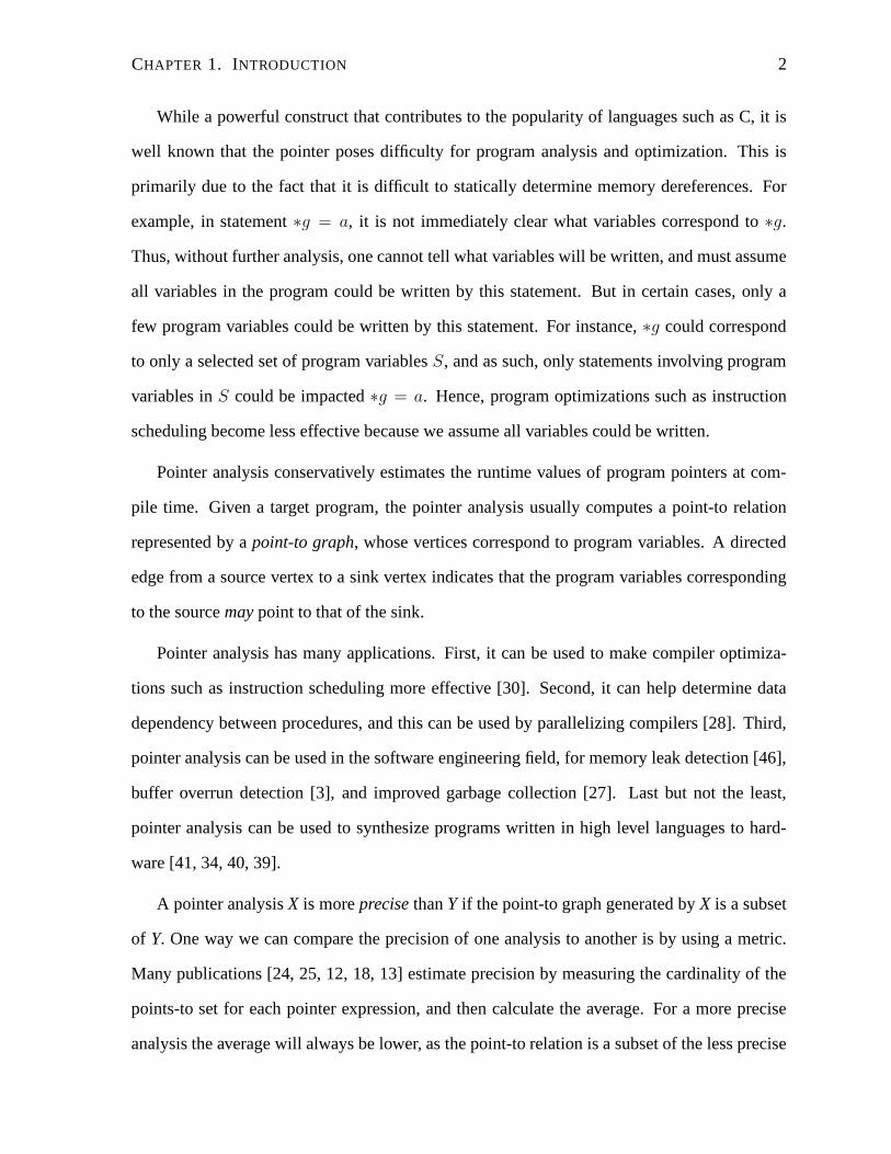
While a powerful construct that contributes to the popularity of languages such as C, it is
well known that the pointer poses difficulty for program analysis and optimization. This is
primarily due to the fact that it is difficult to statically determine memory dereferences. For
example, in statement ∗g = a, it is not immediately clear what variables correspond to ∗g.
Thus, without further analysis, one cannot tell what variables will be written, and must assume
all variables in the program could be written by this statement. But in certain cases, only a
few program variables could be written by this statement. For instance, ∗g could correspond
to only a selected set of program variables S, and as such, only statements involving program
variables in S could be impacted ∗g = a. Hence, program optimizations such as instruction
scheduling become less effective because we assume all variables could be written.
Pointer analysis conservatively estimates the runtime values of program pointers at com-
pile time. Given a target program, the pointer analysis usually computes a point-to relation
represented by a point-to graph, whose vertices correspond to program variables. A directed
edge from a source vertex to a sink vertex indicates that the program variables corresponding
to the source may point to that of the sink.
Pointer analysis has many applications. First, it can be used to make compiler optimiza-
tions such as instruction scheduling more effective [30]. Second, it can help determine data
dependency between procedures, and this can be used by parallelizing compilers [28]. Third,
pointer analysis can be used in the software engineering field, for memory leak detection [46],
buffer overrun detection [3], and improved garbage collection [27]. Last but not the least,
pointer analysis can be used to synthesize programs written in high level languages to hard-
ware [41, 34, 40, 39].
A pointer analysis X is more precise than Y if the point-to graph generated by X is a subset
of Y. One way we can compare the precision of one analysis to another is by using a metric.
Many publications [24, 25, 12, 18, 13] estimate precision by measuring the cardinality of the
points-to set for each pointer expression, and then calculate the average. For a more precise
analysis the average will always be lower, as the point-to relation is a subset of the less precise
CHAPTER 1. INTRODUCTION 3
point-to relation.
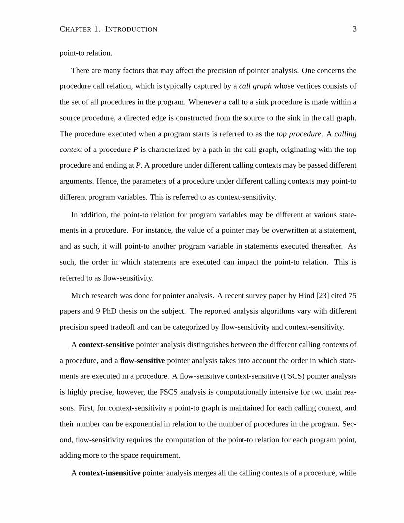
There are many factors that may affect the precision of pointer analysis. One concerns the
procedure call relation, which is typically captured by a call graph whose vertices consists of
the set of all procedures in the program. Whenever a call to a sink procedure is made within a
source procedure, a directed edge is constructed from the source to the sink in the call graph.
The procedure executed when a program starts is referred to as the top procedure. A calling
context of a procedure P is characterized by a path in the call graph, originating with the top
procedure and ending at P. A procedure under different calling contexts may be passed different
arguments. Hence, the parameters of a procedure under different calling contexts may point-to
different program variables. This is referred to as context-sensitivity.
In addition, the point-to relation for program variables may be different at various state-
ments in a procedure. For instance, the value of a pointer may be overwritten at a statement,
and as such, it will point-to another program variable in statements executed thereafter. As
such, the order in which statements are executed can impact the point-to relation. This is
referred to as flow-sensitivity.
Much research was done for pointer analysis. A recent survey paper by Hind [23] cited 75
papers and 9 PhD thesis on the subject. The reported analysis algorithms vary with different
precision speed tradeoff and can be categorized by flow-sensitivity and context-sensitivity.
A context-sensitive pointer analysis distinguishes between the different calling contexts of
a procedure, and a flow-sensitive pointer analysis takes into account the order in which state-
ments are executed in a procedure. A flow-sensitive context-sensitive (FSCS) pointer analysis
is highly precise, however, the FSCS analysis is computationally intensive for two main rea-
sons. First, for context-sensitivity a point-to graph is maintained for each calling context, and
their number can be exponential in relation to the number of procedures in the program. Sec-
ond, flow-sensitivity requires the computation of the point-to relation for each program point,
adding more to the space requirement.
A context-insensitive pointer analysis merges all the calling contexts of a procedure, while

CHAPTER 1. INTRODUCTION 4
a flow-insensitive analysis ignores statement order. The flow-insensitive context-insensitive
(FICI) analysis is able to scale to large programs, but is less precise than the FSCS pointer
analysis. This is partly because the FICI pointer analysis merges point-to relations. Further-
more, the merging is also responsible for the generation of spurious point-to relations since
the point-to graph is used recursively to resolve dereferences of pointers. For instance, in the
statement ∗g = a, we resolve ∗g using the point-to graph. In the FSCS analysis, the program
variables g points-to at the statement ∗g = a will be assigned to point-to a. In the FICI anal-
ysis, the program variables g points-to throughout the program will be assigned to point-to
a.
Thus, there is a tradeoff between precision and efficiency, and the context-sensitive pointer-
analysis algorithms reported so far have some drawbacks. Some pointer analysis algorithms
do not manage to scale to large programs [17, 48]. Other pointer analysis algorithms manage
to scale [18, 16, 18, 16, 13], but their precision is sub-optimal, primarily because they do not
distinguish between all calling contexts. The main reason the context-sensitive analysis does
not scale is the vast number of calling contexts in larger programs. For example, the benchmark
moria with a mere 20 thousand lines of code in the prolangs benchmarks [37], has 320 million
calling contexts.
Recently, the symbolic method has been proposed for pointer analysis [49]. The symbolic
method encodes the pointer analysis problem into the Boolean domain, and currently uses
Binary Decision Diagram (BDD) to represent and manipulate Boolean functions [8]. The
BDD was proposed by Bryant to represent Boolean functions efficiently. They are essentially a
compression of a binary decision tree, achieved by a strict decomposition order and the merging
of isomorphic nodes. BDDs have many desirable properties. First, they are canonical, and thus,
any Boolean operation on the same BDDs will result in an identical BDD. Hence, we can hash
the result BDD, and reuse it whenever the same operands are encountered, a principle similar
to dynamic programming. Second, through the canonical property and aggressive merging,
BDDs are also quite compact. Lastly, since the runtime complexity depends on the size of the
CHAPTER 1. INTRODUCTION 5
BDD, the compactness directly translates into speed efficiency.
Zhu [49] demonstrated that the symbolic method can exploit the properties of the BDD for
pointer analysis, in a context-sensitive analysis for C programs. However, the algorithm did not
scale to large programs because the invocation graph, which determines calling contexts, was
constructed explicitly, and thus had an exponential growth in the number of nodes in relation
to the call graph. Berndl et al [7] independently proposed a flow-insensitive context-insensitive
pointer analysis for Java programs using BDDs. The work demonstrated space efficiency and
scalability, analyzing large Java programs in minutes.
1.2 Contributions
In this thesis, we propose a symbolic algorithm for context sensitive pointer analysis. We make
the following contributions:
• Symbolic Invocation Graph. Most previous methods [17, 48, 49] for context sensi-
tive analysis require the construction of an invocation graph, which can be exponentially
large. We propose the use of BDDs to annotate the call graph edges with Boolean func-
tions to implicitly capture the corresponding invocation edges. Such representation of
the invocation graph leads to the exponential reduction of memory size. In addition, we
show the construction of the invocation graph can be done in polynomial time.
• State Superposition. In contrast to the previous efforts where program states of a proce-
dure under different calling contexts have to be evaluated separately by the application of
transfer functions, we devise a scheme where the the symbolic invocation graph is lever-
aged to collectively compute a superposition of all states of a procedure under different
contexts. This leads to an exponential reduction of analysis runtime in practice.
• Symbolic Transfer Function. We extend our original proposal of symbolic transfer
function in [49], which uses a Boolean function represented by a BDD to capture the
CHAPTER 1. INTRODUCTION 6
program state of a procedure as a function of its caller program state. Our extension
allows the additional parameterization of the callee program state, which enables the
capture of transfer functions in a single pass.
• Common CI/CS symbolic analysis framework. We establish a common, efficient
framework for both context-sensitive and context-insensitive analysis. This not only en-
ables the leverage of transfer functions for the first time to speed up CI analysis, but also
enables the study of speed-accuracy tradeoff among a spectrum of symbolic analysis
methods with different context-sensitivity. To the best of our knowledge, such frame-
works useful in many studies have not been reported for BDD-based pointer analysis.
We implemented the new algorithm and measured its runtime, memory consumption, and
precision. Our implementation computes points-to information for programs written in the C
programming language. In addition, we experimented with various attributes for BDDs, to
obtain insights into the effectiveness of the BDD when used for pointer analysis.
1.3 Thesis Organization
The thesis is organized as follows. In Chapter 2 we review the previous work on pointer
analysis. In Chapter 3 we describe the pointer analysis output, and show and discuss how
the program model is used to generate the points-to relation. Next, in Chapter 4 we present
the symbolic invocation graph, and its construction algorithm. Lastly, in Chapters 5 and 6 we
present the experimental results and the conclusion.
Chapter 2
Related Work
For pointer analysis, mainly two metrics are used to evaluate a given algorithm. One met-
ric is the scalability of the pointer analysis to large programs. This is important since many
applications need to analyze large programs. The other metric is the precision of the pointer
analysis, which can be impacted by a number of factors. One of these factors is the modeling
of the memory space, as the address of a program variable is usually represented by an abstract
structure called a block. Pointer analysis algorithms tend to be less precise when they represent
more program variables by a given block. Another factor is the degree of context-sensitivity
and flow-sensitivity in the algorithm. For instance, we may choose to distinguish between only
certain calling contexts of procedures in the context-sensitive pointer analysis [13, 18].
Andersen [4] proposed a flow-insensitive context-insensitive pointer analysis. In his anal-
ysis, a block was assigned to each stack and global variable. In addition, the analysis distin-
guished between heap locations allocated at different statements in the program. The analysis
generated point-to relations between the dereferences of program variables, called constraints.
The set of constraints can be abstracted as a constraint graph, whose vertices correspond to
the various dereferences of program variables. Generating the point-to graph is typically done
by performing a transitive closure of the constraint graph. For example, consider a C program
made of two statements, a = &b and b = &c. We let Ta, Tb, Tc be the values of a, b, and c
7
CHAPTER 2. RELATED WORK 8
respectively. In addition, we let T∗a be the value of the dereference of a. Clearly, a points-to
b, and b points-to c, partly denoted by the constraints Ta ⊇ {b} and Tb ⊇ {c}. From these
constraints, we can resolve the expression ∗a, denoted by T∗a ⊇ ∗Ta. This is done by propa-
gating the point-to values of the previous constraints to derive T∗a ⊇ {c}. It was shown that
Andersen’s analysis has a cubic complexity.
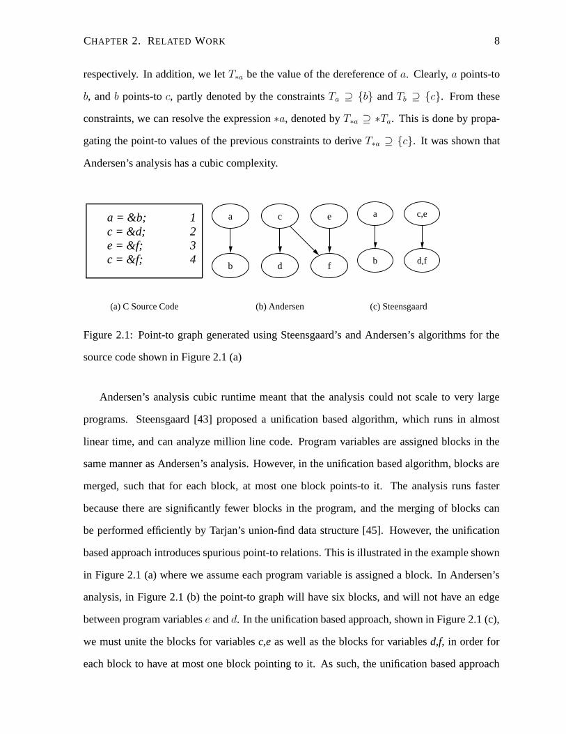
a = &b; 1c = &d; 2e = &f; 3c = &f; 4
(a) C Source Code
a
b
c
d f
e
(b) Andersen
a
b
c,e
d,f
(c) Steensgaard
Figure 2.1: Point-to graph generated using Steensgaard’s and Andersen’s algorithms for the
source code shown in Figure 2.1 (a)
Andersen’s analysis cubic runtime meant that the analysis could not scale to very large
programs. Steensgaard [43] proposed a unification based algorithm, which runs in almost
linear time, and can analyze million line code. Program variables are assigned blocks in the
same manner as Andersen’s analysis. However, in the unification based algorithm, blocks are
merged, such that for each block, at most one block points-to it. The analysis runs faster
because there are significantly fewer blocks in the program, and the merging of blocks can
be performed efficiently by Tarjan’s union-find data structure [45]. However, the unification
based approach introduces spurious point-to relations. This is illustrated in the example shown
in Figure 2.1 (a) where we assume each program variable is assigned a block. In Andersen’s
analysis, in Figure 2.1 (b) the point-to graph will have six blocks, and will not have an edge
between program variables e and d. In the unification based approach, shown in Figure 2.1 (c),
we must unite the blocks for variables c,e as well as the blocks for variables d,f, in order for
each block to have at most one block pointing to it. As such, the unification based approach

CHAPTER 2. RELATED WORK 9
produces an additional point-to edge between program variables e and d. As it was shown, the
unification based pointer analysis derives certain point-to edges through the merging operation,
degrading precision. In large programs, the merging typically occurs on a very large scale,
producing a very large number of spurious point-to relations.
Fahndrich, Foster, Su, and Aiken [19] proposed a flow-insensitive context-insensitive pointer
analysis. They improved on the runtime of Andersen’s [4] pointer analysis by collapsing cyclic
constraints, and by propagating constraints lazily. Intuitively, the authors propose to detect
pointers that point-to the same program variables at various dereferences, and evaluate their
constraints together. In addition, by not performing the transitive closure for the entire con-
straint graph, they can avoid the overhead caused by evaluating cyclic constraints. Instead,
cyclic constraints are first identified and collapsed into a single block. They demonstrated or-
ders of magnitude improvement in analysis runtime due to collapsing cyclic constraints, and
a further improvement due to propagating constraints lazily. Rountev and Chandra [35] pro-
posed a more aggressive algorithm collapsing cyclical constraints, where they propagate the
label (block), and detect additional variables with identical points-to information. In particular
they managed to scale to 500 KLOC program. Heinze and Tardieu [22], proposed a demand
driven analysis, computing only the points-to results the client asks for. They showed this
analysis can analyze million line code in seconds.
In addition to improving the runtime of pointer analysis, the precision could be improved
by introducing flow-sensitivity and context-sensitivity. Emami, Ghiya, and Hendren [17] pro-
posed a flow-sensitive context-sensitive pointer analysis for C programs. The analysis assigns
distinct blocks to stack variables including locals, parameters, and globals along with unknown
indirect accesses through these variables. In addition, the heap was assigned one abstract mem-
ory block, and each procedures was assigned an abstract memory block to determine the targets
of indirect calls. The analysis also computes must point-to relations, which detect the values
that pointers are guaranteed to have. The must point-to relation was used to kill point-to rela-
tions for dereferenced blocks.
CHAPTER 2. RELATED WORK 10
Emami et al. propose using the invocation graph instead of the call graph for the context-
sensitive pointer analysis. The invocation graph is generated by expanding the call graph, du-
plicating each non-recursive call target. Hence, in a context-sensitive analysis, each procedure
is expanded into all its invocations. The advantage gained is that the locals and parameters of a
procedure are assigned a different abstract block for each invocation. Hence, since they distin-
guish between the parameters and locals at different invocations, they can distinguish between
the arguments passed in from different call sites. Although this analysis improves precision
in relation to the context-insensitive flow-insensitive pointer analysis, the programs analyzed
were only few thousand lines of code.
Wilson and Lam [48] noticed that many of the calling contexts were quite similar in terms
of alias patterns between the parameters. As such, they proposed the use of partial transfer
function (PTF) to capture the points-to information for each procedure. The PTF does this
by using blocks called initials to represent initial point-to information of parameters, and
uses the PTF to derive the final point-to information of the procedure. In order to derive the
point-to information for a procedure, the actual arguments are substituted into the PTF. The
advantage of the PTF is that a particular PTF for a procedure can be reused whenever the same
alias patterns occur. In this analysis they allocated each stack variable and global an abstract
memory location. In addition, they distinguished between heap blocks allocated at different
sites in the program. The pointer analysis was shown to run on benchmarks as large as five
thousand lines of code.
The context-sensitive pointer analysis algorithms discussed so far do not scale because they
require the construction of the invocation graph, which is of exponential complexity in relation
to the number of procedures. Fahndric, Rehof, and Das [18], proposed a one-level unification
based context-sensitive pointer analysis. This analysis proposes to distinguish between the
incoming calls to a given procedure, rather than expand each path in the call graph. The
authors showed that this analysis can analyze hundreds of thousands of LOC in minutes, and
showed precision improvements over the flow-insensitive context-insensitive unification based
CHAPTER 2. RELATED WORK 11
analysis.
Chaterjee, Ryder, and Landi [12] proposed a modular context-sensitive pointer analysis,
using the same block allocation as Wilson and Lam [48], but fully summarizing each procedure
using a transfer function. By detecting strongly connected components in the call graph, and
analyzing them separately they showed space improvements, but no results on benchmarks
larger than 5000 lines of code. Cheng and Hwu [13] extended [12] by implementing an access
path based approach, and partial context-sensitivity, distinguishing between the arguments at
only selected procedures. They demonstrated scalability to hundreds of thousands of LOC.
There are many ways to represent logic functions, the concept of Binary Decision Diagram
(BDD) was first proposed by Akers [2]. Bryant’s Reduced Order BDD (ROBDD) [8] made
this representation successful through its compactness and canonical property. The BDD was
applied to a wide range of tasks, including simulation, synthesis and formal verification in the
CAD community. McMillan et al. [11] and Coudert et al. [14] were the first to introduce BDD
into the model checking of sequential circuits, which can be abstracted as finite state machines.
Their pioneer work replaces the explicit state enumeration by implicit state enumeration us-
ing BDDs. This key concept, complemented by further improvements [9, 15, 10, 33], was
responsible for the first application of model checking to practical problems.
Other efforts in using a Boolean framework for program analysis were made. Sagiv, Reps,
and Wilhelm [38] applied this principle to shape analysis, while Ball and Millstein [5] did pred-
icate abstraction. However, the number of Boolean variables introduced in these frameworks
is proportional to the number of subjects of interest.
The application of the BDD technique to pointer analysis problem was first reported by
Zhu in [49], a context-sensitive pointer analysis for C programs, where memory blocks are
logarithmically encoded into the Boolean domain. The concept of symbolic transfer function
and the use of BDD image computation to perform program state query was proposed and its
speed efficiency was demonstrated. Berndl et al. reported a context-insensitive pointer anal-
ysis algorithm using BDD in [7], where the space efficiency, and therefore better scalability
CHAPTER 2. RELATED WORK 12
than the classical methods for analyzing Java programs was demonstrated. Lhotak and Hen-
dren [31] built a relational database abstraction on top of the low-level BDD manipulation to
facilitate symbolic program analysis. This abstraction simplifies the integration of multiple
program analysis techniques using BDDs. Whaley and Lam [47] reported another method for
context-sensitive pointer analysis using BDD for Java programs. They encode the invocation
graph using BDDs, and apply the algorithm by Berndl et al. [7] to the context-sensitive graph,
producing a context-sensitive pointer analysis. Their analysis scales to large Java programs.
Zhu and Calman [50] proposed a context-sensitive pointer analysis using BDDs for C pro-
grams. The algorithm proposed encodes the complete transfer function for each procedure and
the invocation graph using BDDs. It then applies the transfer function using the invocation
graph, producing the context-sensitive pointer analysis.

Chapter 3
Symbolic Program Modeling
This chapter is organized as follows. In Section 3.1 we explain how a relation can be repre-
sented by a Boolean function. In Section 3.2 we describe how the points-to graph is represented
symbolically. In Section 3.3 we discuss the transfer function, which is used to compute the
point-to graph. In Section 3.4 we discuss Binary Decision Diagrams and their use in pointer
analysis. In Section 3.5 we derive a mathematical model for the program and explain how
the pointer analysis can be solved using recurrence equations. Lastly, in Section 3.6 and Sec-
tion 3.7 we discuss the state query and transfer function application respectively, which are
used in computing the recurrence equations.
3.1 Preliminary
A Boolean constant is either true or false. A Boolean variable is a symbol whose value is a
Boolean constant. The logic connectives , ·, + correspond to the negation, conjunction, and
disjunction operators respectively. A Boolean function can be a Boolean constant, Boolean
variable, the negation of a Boolean function, and lastly, the conjunction or disjunction of two
Boolean functions. A literal is a Boolean variable or its negation. A truth assignment τ evalu-
ates each Boolean variable in a set as true or false. If τ assigns a value to each Boolean variable
in a Boolean function f, then under τ , f evaluates to true or false.
13
CHAPTER 3. SYMBOLIC PROGRAM MODELING 14
From a set of Boolean variables, U = {x0, x1, ..., xm−1}, we can derive a conjunction cj of
m literals, called a minterm. Notice that since each distinct minterm is satisfied by only one τ
over U , the set of minterms are orthogonal. In other words, for any two minterms u, v spanned
by U , u · v = 0 if u 6= v.
Let A1, A2, ..., An be sets, then an n-ary relation on these sets would be a subset of A1 ×
A2 × ... × An. We call A1, A2, ..., An the domains of the relation, and n is the degree of
the relation. To represent relations we use a set of Boolean variables for each domain. Let
A1, A2, ..., An be the domains of the n-ary relation, and respectively, U 1, U2, ..., Un are sets of
Boolean variables for these domains such that U i ∩ U j = � if i 6= j and |U i| = dlog2 |Ai|e for
1 ≤ i ≤ n. The jth Boolean variable in U i is referred to as uij. Without loss of generality we
assume that the elements in each domain Ai are unique numbers, ranging from 0 to |Ai| − 1.
The minterm for e ∈ Ai is derived by its binary representation∑
j bj2j, where bj is the jth
bit of e. In the derivation we will use the Boolean variables in U i, inserting uij or ui
j if bj is
1 or 0 respectively. All variables are substituted because the size of U i is designed to have
as many variables as there are bits in the binary representation of each number in Ai. Note
that the minterm created for e ∈ Ai, referred to as U ie, is constructed to satisfy only one τ ,
corresponding to the unique number e. Note also that we can create a relation minterm by a
conjunction of the minterms U 1e1
, U2e2
, ..., Unen
, where 〈e1, e2, ..., en〉 is a subset of the relation.
We can represent a relation by a disjunction of relation minterms.
Example 1 Consider the domains A1 = A2 = {0, 1, 2, 3, 4, 5, 6, 7} and the relation R =
{〈0, 1〉, 〈1, 6〉} ⊂ A1 × A2. Then, to represent R, we create two sets of Boolean variables,
U1 = {u10, u
11, u
12}, and U 2 = {u2
0, u21, u
22}. In this example, the elements 0 and 1 in A1 are
encoded using Boolean variables in U 1 by u10u
11u
12 and u1
0u11u
12 respectively, which corresponds
to their 3 bit binary representation. The relation R is then encoded symbolically by the Boolean
function U10 U2
1 + U11 U2
6 = u10u
11u
12u
20u
21u
22 + u1
0u11u
12u
20u
21u
22.
With the symbolic representation described above, set union and set intersection are equiv-
alent to Boolean disjunction and conjunction, respectively, of the symbolic representation of a
CHAPTER 3. SYMBOLIC PROGRAM MODELING 15
set. Thus, from here on, we do not distinguish a set or relation from their symbolic representa-
tion.
It is possible to find subsets of a relation, relevant to elements in a certain domain. This
can be done by creating a disjunction of the minterms D for the respective elements, and
multiplying them by the relation R. Since the minterm for each element e ∈ D is orthogonal
to the minterm for any other element g 6∈ D in its domain, parts of the relation involving g will
evaluate to � when multiplied by the disjunction of minterms for D. As such, the result of the
multiplication is S ⊆ R, such that only relation minterms involving D will be part of S.
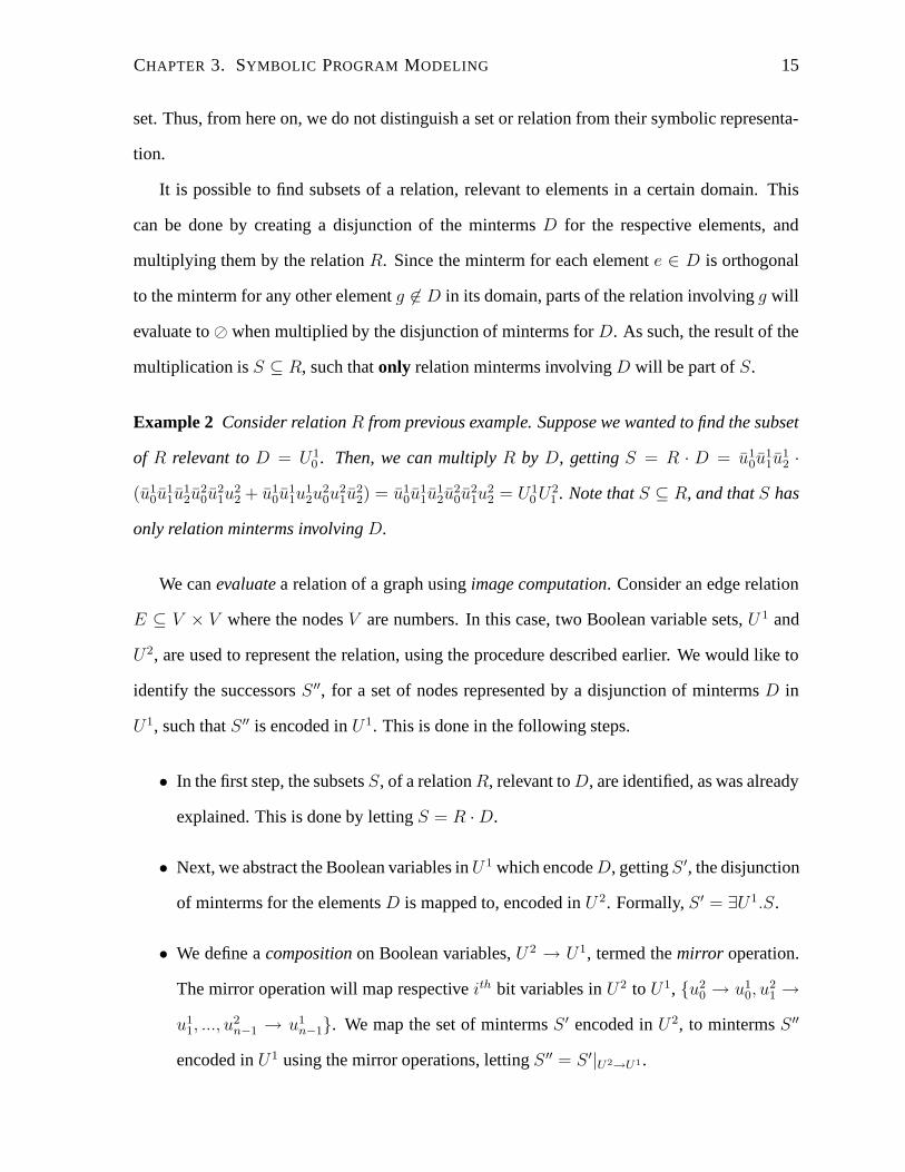
Example 2 Consider relation R from previous example. Suppose we wanted to find the subset
of R relevant to D = U 10 . Then, we can multiply R by D, getting S = R · D = u1
0u11u
12 ·
(u10u
11u
12u
20u
21u
22 + u1
0u11u
12u
20u
21u
22) = u1
0u11u
12u
20u
21u
22 = U1
0 U21 . Note that S ⊆ R, and that S has
only relation minterms involving D.
We can evaluate a relation of a graph using image computation. Consider an edge relation
E ⊆ V × V where the nodes V are numbers. In this case, two Boolean variable sets, U 1 and
U2, are used to represent the relation, using the procedure described earlier. We would like to
identify the successors S ′′, for a set of nodes represented by a disjunction of minterms D in
U1, such that S ′′ is encoded in U 1. This is done in the following steps.
• In the first step, the subsets S, of a relation R, relevant to D, are identified, as was already
explained. This is done by letting S = R · D.
• Next, we abstract the Boolean variables in U 1 which encode D, getting S ′, the disjunction
of minterms for the elements D is mapped to, encoded in U 2. Formally, S ′ = ∃U1.S.
• We define a composition on Boolean variables, U 2 → U1, termed the mirror operation.
The mirror operation will map respective ith bit variables in U 2 to U1, {u20 → u1
0, u21 →
u11, ..., u
2n−1 → u1
n−1}. We map the set of minterms S ′ encoded in U 2, to minterms S ′′
encoded in U 1 using the mirror operations, letting S ′′ = S ′|U2→U1 .
CHAPTER 3. SYMBOLIC PROGRAM MODELING 16
Note that it is possible to identify the graph nodes reachable form D by repeated application
of the three steps above. This fact is utilized in Section 3.6, where the image computation along
with the mirror operation will allow us to perform point-to graph queries.
Example 3 Consider the domain V = A1 = A2 = {0, 1, 2, 3, 4, 5, 6, 7}, the relation R =
{〈0, 1〉, 〈1, 6〉} ⊂ A1 × A2 = V × V , and the minterm D = U 10 . We can identify the elements
D is mapped to, and convert them to the domain of U 1. This is done by first abstracting
the Boolean variables in U 1 for S, producing S ′ = ∃U1.[u10u
11u
12u
20u
21u
22] = u2
0u21u
22 = U2
1 .
Next, we can apply the mirror operation to convert the minterm from U 2 to U1, denoted by
S ′′ = u20u
21u
22|U2→U1 = u1
0u11u
12 = U1
1 . Thus, using these operations, we identified U 10 is
mapped to U 21 , and then the mirror operation was used to convert U 2
1 to U11 . This procedure
can be performed again, taking ∗S ′′ = (∃U1[S ′′ · R])|U2→U1 = U16 .
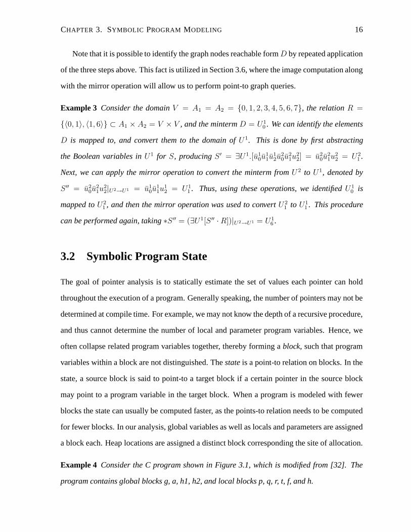
3.2 Symbolic Program State
The goal of pointer analysis is to statically estimate the set of values each pointer can hold
throughout the execution of a program. Generally speaking, the number of pointers may not be
determined at compile time. For example, we may not know the depth of a recursive procedure,
and thus cannot determine the number of local and parameter program variables. Hence, we
often collapse related program variables together, thereby forming a block, such that program
variables within a block are not distinguished. The state is a point-to relation on blocks. In the
state, a source block is said to point-to a target block if a certain pointer in the source block
may point to a program variable in the target block. When a program is modeled with fewer
blocks the state can usually be computed faster, as the points-to relation needs to be computed
for fewer blocks. In our analysis, global variables as well as locals and parameters are assigned
a block each. Heap locations are assigned a distinct block corresponding the site of allocation.
Example 4 Consider the C program shown in Figure 3.1, which is modified from [32]. The
program contains global blocks g, a, h1, h2, and local blocks p, q, r, t, f, and h.

CHAPTER 3. SYMBOLIC PROGRAM MODELING 17
char *g, a, h1, h2; 1void main() { 2
char *p, *q; 3S0: alloc( &p, &h1 ); 4S1: getg( &q ); 5
g = &a; 6} 7
8void getg( char** r ) { 9
char **t = &g; 10if( g == NULL ) 11
S2: alloc( t, &h2 ); 12*r = *t; 13} 14
15void alloc( char** f, char *h ) { 16
*f = h; 17} 18
Figure 3.1: C source code
The program state is often abstracted as a point-to graph 〈B, E〉, whose vertices B rep-
resent the set of blocks, and an edge 〈u, v〉 ∈ E from block u to block v indicates that it is
possible that block u points-to block v. The set of all edges defines the point-to relation.
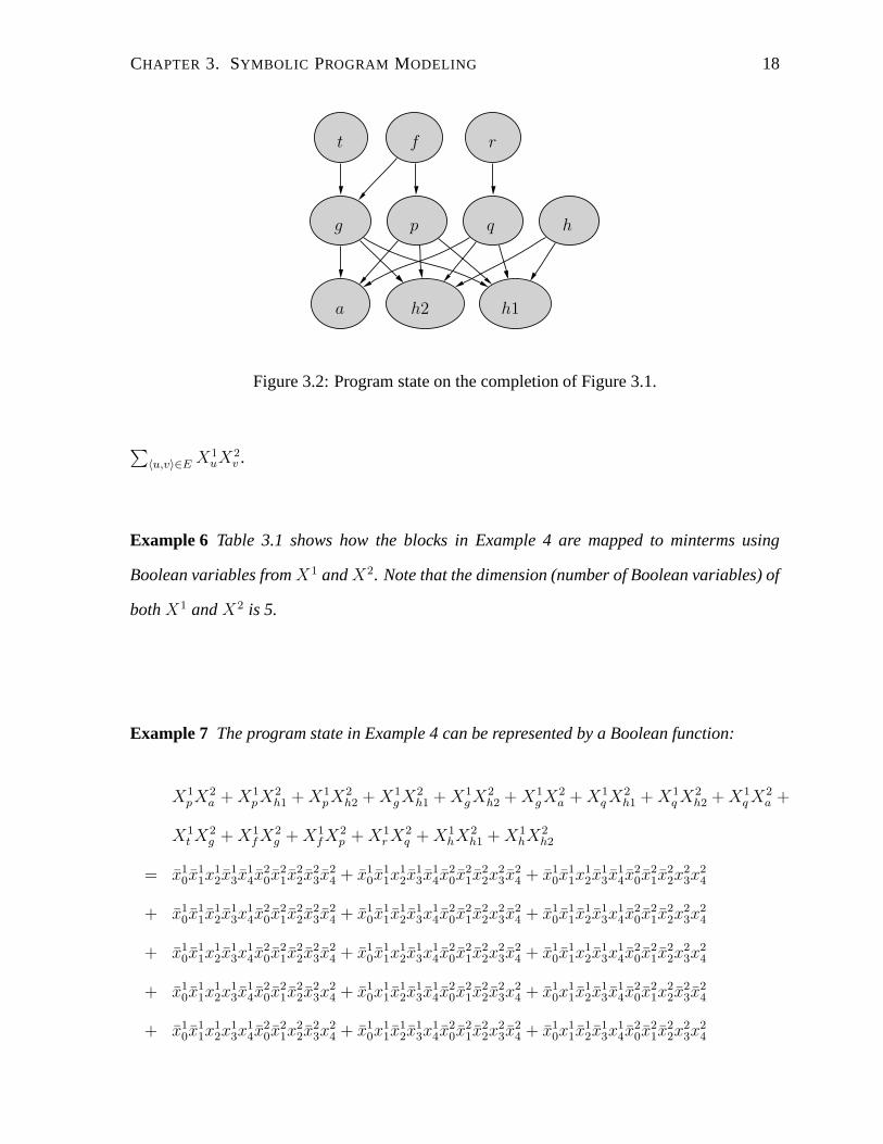
Example 5 Figure 3.2 shows a point-to graph capturing the program state after the comple-
tion of the main procedure in Figure 3.1.
To represent the relation E ⊆ B × B we create two Boolean sets X 1 = {x10, x
11, ..., x
1n−1}
and X2 = {x20, x
21, ..., x
2n−1}, to derive minterms for blocks. We let |X1| = |X2| = dlog2 |B|e,
and assume that each block u is characterized by a number. As such, we can derive the minterm
for u using its binary representation, and Boolean variables in either X 1 or X2. Assuming a
block u points to a block v, we represent the point-to relation by the relation minterm X 1uX2
v .
In other words, we capture the point-to edge 〈u, v〉 in the point-to graph by a Boolean product
X1uX2
v . Thus, given a program state represented by E, the point-to graph is represented by
CHAPTER 3. SYMBOLIC PROGRAM MODELING 18
PSfrag replacements
x20
x10
x21
x11
x22
x12
x23
x13
x24
x14
y1
y∗1
y2
y∗2
y3
y∗3
λ0
θ0
λ1
θ1
θ2
λ2
θ3
λ∗0
θ∗0
λ∗1
θ∗1
θ∗2
λ∗2
θ∗3
a
g
rt
p q
h1h2
f
h
m
p1
q1
Figure 3.2: Program state on the completion of Figure 3.1.
∑〈u,v〉∈E X1
uX2v .
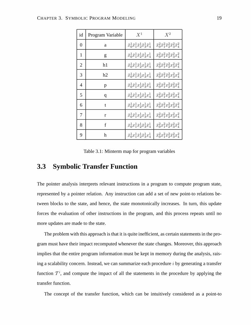
Example 6 Table 3.1 shows how the blocks in Example 4 are mapped to minterms using
Boolean variables from X1 and X2. Note that the dimension (number of Boolean variables) of
both X1 and X2 is 5.
Example 7 The program state in Example 4 can be represented by a Boolean function:
X1pX2
a + X1pX2
h1 + X1pX2
h2 + X1g X2
h1 + X1gX2
h2 + X1g X2
a + X1q X2
h1 + X1q X2
h2 + X1q X2
a +
X1t X2
g + X1fX2
g + X1fX2
p + X1r X2
q + X1hX2
h1 + X1hX2
h2
= x10x
11x
12x
13x
14x
20x
21x
22x
23x
24 + x1
0x11x
12x
13x
14x
20x
21x
22x
23x
24 + x1
0x11x
12x
13x
14x
20x
21x
22x
23x
24
+ x10x
11x
12x
13x
14x
20x
21x
22x
23x
24 + x1
0x11x
12x
13x
14x
20x
21x
22x
23x
24 + x1
0x11x
12x
13x
14x
20x
21x
22x
23x
24
+ x10x
11x
12x
13x
14x
20x
21x
22x
23x
24 + x1
0x11x
12x
13x
14x
20x
21x
22x
23x
24 + x1
0x11x
12x
13x
14x
20x
21x
22x
23x
24
+ x10x
11x
12x
13x
14x
20x
21x
22x
23x
24 + x1
0x11x
12x
13x
14x
20x
21x
22x
23x
24 + x1
0x11x
12x
13x
14x
20x
21x
22x
23x
24
+ x10x
11x
12x
13x
14x
20x
21x
22x
23x
24 + x1
0x11x
12x
13x
14x
20x
21x
22x
23x
24 + x1
0x11x
12x
13x
14x
20x
21x
22x
23x
24
CHAPTER 3. SYMBOLIC PROGRAM MODELING 19
id Program Variable X1 X2
0 a x10x
11x
12x
13x
14 x2
0x21x
22x
23x
24
1 g x10x
11x
12x
13x
14 x2
0x21x
22x
23x
24
2 h1 x10x
11x
12x
13x
14 x2
0x21x
22x
23x
24
3 h2 x10x
11x
12x
13x
14 x2
0x21x
22x
23x
24
4 p x10x
11x
12x
13x
14 x2
0x21x
22x
23x
24
5 q x10x
11x
12x
13x
14 x2
0x21x
22x
23x
24
6 t x10x
11x
12x
13x
14 x2
0x21x
22x
23x
24
7 r x10x
11x
12x
13x
14 x2
0x21x
22x
23x
24
8 f x10x
11x
12x
13x
14 x2
0x21x
22x
23x
24
9 h x10x
11x
12x
13x
14 x2
0x21x
22x
23x
24
Table 3.1: Minterm map for program variables
3.3 Symbolic Transfer Function
The pointer analysis interprets relevant instructions in a program to compute program state,
represented by a pointer relation. Any instruction can add a set of new point-to relations be-
tween blocks to the state, and hence, the state monotonically increases. In turn, this update
forces the evaluation of other instructions in the program, and this process repeats until no
more updates are made to the state.
The problem with this approach is that it is quite inefficient, as certain statements in the pro-
gram must have their impact recomputed whenever the state changes. Moreover, this approach
implies that the entire program information must be kept in memory during the analysis, rais-
ing a scalability concern. Instead, we can summarize each procedure i by generating a transfer
function T i, and compute the impact of all the statements in the procedure by applying the
transfer function.
The concept of the transfer function, which can be intuitively considered as a point-to

CHAPTER 3. SYMBOLIC PROGRAM MODELING 20
relation parameterized over different calling contexts, has been widely used [48, 12, 13]. The
parameters of the transfer function do not necessarily correspond to the parameters of the
procedure. In fact, dereferences of any parameter, global, and local within the procedure can
be a transfer function parameter. A memory dereference can be characterized by the notion
of access path 〈b, l〉, where b is the root memory block, and l is the level of dereferences. An
access path with the form 〈b, 0〉 is trivial and always resolves to the constant address value b,
whereas an access path with the form 〈b, 1〉 represents the value stored in b. After the transfer
functions of all program procedure are derived, they can be applied at their corresponding call
sites by substituting the parameters, or the unknowns, with the known program state.
In [49] we introduce the notion of initial state blocks, each of which corresponds to the
set of possible values of a memory dereference before entering the procedure. An initial state
block is treated as if it was a separate memory block.
One problem with only using initial blocks as transfer function parameters is that the trans-
fer function of a procedure depends very much on the transfer functions of its callees. To make
sure that the point-to information of a procedure is evaluated as late as possible, we introduce
final state blocks, which represent possible values of a memory dereference before leaving the
procedure. Again, we use disjoint minterms with Boolean variables from X 1 and X2 to encode
initial and final state blocks. We follow the convention that the minterms λk and θk represent
the initial and final state block for memory dereference k respectively.
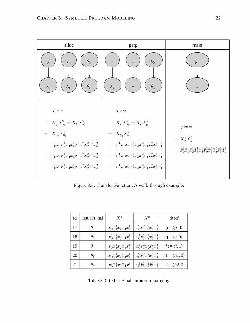
Example 8 Consider the procedure alloc in Example 4, where the parameters f and h are
dereferenced. Since the value of f and h are unknown, we cannot determine the memory blocks
to be updated. With the introduction of the initial state blocks λ0 and λ1, and the final state
blocks θ0 and θ1, the procedure can be summarized with a transfer function as shown in the
point-to graph of Figure 3.3. Similarly, we can obtain the transfer function of procedure getg in
Example 4 in Figure 3.3 where memory dereference 2 corresponds to *r and memory derefer-
ence 3 corresponds to **t1. The introduced initial and final blocks can be encoded as minterms
1Note that here we follow the convention of writing L-values, thus the R-value *t at line 14 of Example 4 is
CHAPTER 3. SYMBOLIC PROGRAM MODELING 21
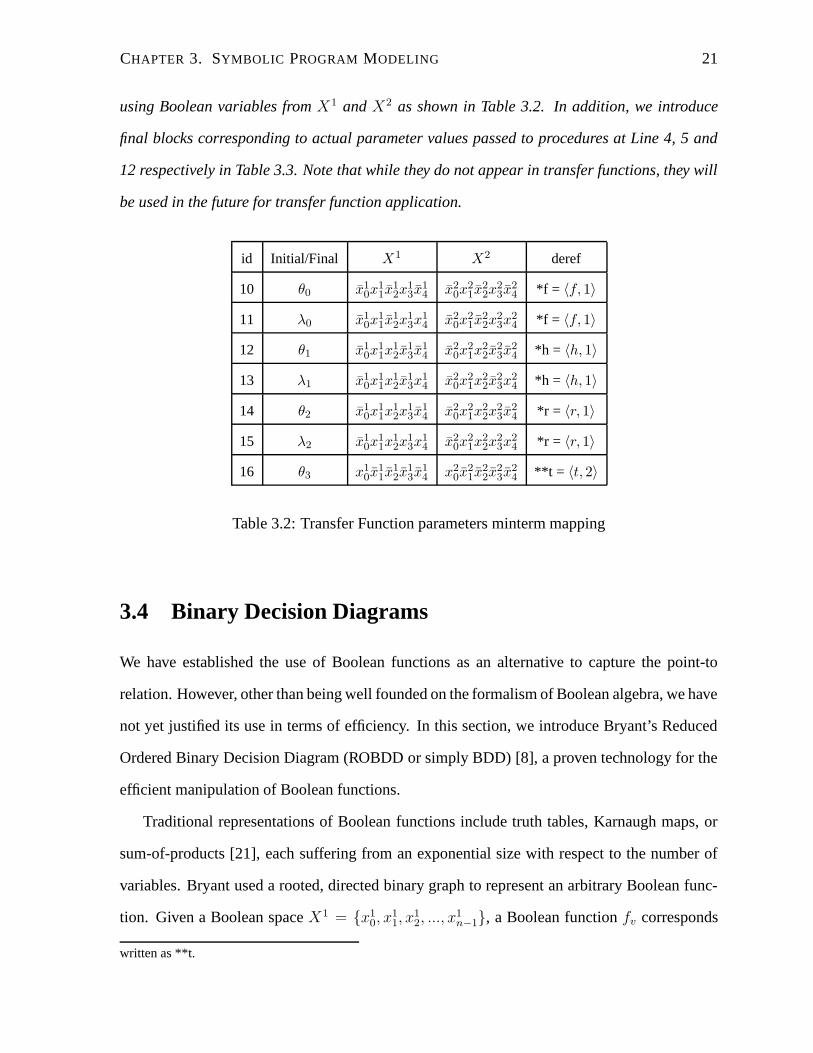
using Boolean variables from X1 and X2 as shown in Table 3.2. In addition, we introduce
final blocks corresponding to actual parameter values passed to procedures at Line 4, 5 and
12 respectively in Table 3.3. Note that while they do not appear in transfer functions, they will
be used in the future for transfer function application.
id Initial/Final X1 X2 deref
10 θ0 x10x
11x
12x
13x
14 x2
0x21x
22x
23x
24 *f = 〈f, 1〉
11 λ0 x10x
11x
12x
13x
14 x2
0x21x
22x
23x
24 *f = 〈f, 1〉
12 θ1 x10x
11x
12x
13x
14 x2
0x21x
22x
23x
24 *h = 〈h, 1〉
13 λ1 x10x
11x
12x
13x
14 x2
0x21x
22x
23x
24 *h = 〈h, 1〉
14 θ2 x10x
11x
12x
13x
14 x2
0x21x
22x
23x
24 *r = 〈r, 1〉
15 λ2 x10x
11x
12x
13x
14 x2
0x21x
22x
23x
24 *r = 〈r, 1〉
16 θ3 x10x
11x
12x
13x
14 x2
0x21x
22x
23x
24 **t = 〈t, 2〉
Table 3.2: Transfer Function parameters minterm mapping
3.4 Binary Decision Diagrams
We have established the use of Boolean functions as an alternative to capture the point-to
relation. However, other than being well founded on the formalism of Boolean algebra, we have
not yet justified its use in terms of efficiency. In this section, we introduce Bryant’s Reduced
Ordered Binary Decision Diagram (ROBDD or simply BDD) [8], a proven technology for the
efficient manipulation of Boolean functions.
Traditional representations of Boolean functions include truth tables, Karnaugh maps, or
sum-of-products [21], each suffering from an exponential size with respect to the number of
variables. Bryant used a rooted, directed binary graph to represent an arbitrary Boolean func-
tion. Given a Boolean space X1 = {x10, x
11, x
12, ..., x
1n−1}, a Boolean function fv corresponds
written as **t.
CHAPTER 3. SYMBOLIC PROGRAM MODELING 22
alloc getg main
PSfrag replacementsx2
0x1
0x2
1x1
1x2
2x1
2x2
3x1
3x2
4x1
4y1y∗
1y2y∗
2y3y∗
3
λ0
θ0
λ1 θ1
θ2λ2θ3λ∗
0θ∗0λ∗
1θ∗1θ∗2λ∗
2θ∗3agrtpq
h1h2
f h
mp1q1
PSfrag replacementsx2
0x1
0x2
1x1
1x2
2x1
2x2
3x1
3x2
4x1
4y1y∗
1y2y∗
2y3y∗
3λ0θ0λ1θ1
θ2
λ2 θ3
λ∗0
θ∗0λ∗
1θ∗1θ∗2λ∗
2θ∗3a
g
r tpq
h1h2fhm
p1q1
PSfrag replacementsx2
0x1
0x2
1x1
1x2
2x1
2x2
3x1
3x2
4x1
4y1y∗
1y2y∗
2y3y∗
3λ0θ0λ1θ1θ2λ2θ3λ∗
0θ∗0λ∗
1θ∗1θ∗2λ∗
2θ∗3
a
grtpq
h1h2fhm
p1q1
T alloc
= X1f X2
λ0+ X1
hX2λ1
+ X1θ0
X2θ1
= x10x
11x
12x
13x
14x
20x
21x
22x
23x
24
+ x10x
11x
12x
13x
14x
20x
21x
22x
23x
24
+ x10x
11x
12x
13x
14x
20x
21x
22x
23x
24
T getg
= X1r X2
λ2+ X1
t X2g
+ X1θ2
X2θ3
= x10x
11x
12x
13x
14x
20x
21x
22x
23x
24
+ x10x
11x
12x
13x
14x
20x
21x
22x
23x
24
+ x10x
11x
12x
13x
14x
20x
21x
22x
23x
24
T main
= X1gX2
a
= x10x
11x
12x
13x
14x
20x
21x
22x
23x
24
Figure 3.3: Transfer Function, A walk-through example.
id Initial/Final X1 X2 deref
17 θ4 x10x
11x
12x
13x
14 x2
0x21x
22x
23x
24 p = 〈p, 0〉
18 θ5 x10x
11x
12x
13x
14 x2
0x21x
22x
23x
24 q = 〈q, 0〉
19 θ6 x10x
11x
12x
13x
14 x2
0x21x
22x
23x
24 *t = 〈t, 1〉
20 θ7 x10x
11x
12x
13x
14 x2
0x21x
22x
23x
24 h1 = 〈h1, 0〉
21 θ8 x10x
11x
12x
13x
14 x2
0x21x
22x
23x
24 h2 = 〈h2, 0〉
Table 3.3: Other Finals minterm mapping
CHAPTER 3. SYMBOLIC PROGRAM MODELING 23
to a graph rooted at graph node v. Each node in the graph is characterized by an index i, cor-
responding to a Boolean variable x1i , as well as its negative cofactor flow and positive cofactor
fhigh, each of which is by itself a Boolean function, and therefore a graph node. Logically,
fv is related to its two cofactors by Shannon expansion fv = xiflow + xifhigh. Two outstand-
ing nodes, called the terminal nodes, represent the constant logic value 0 and 1. The terminal
nodes are assumed to have an index of infinity. By imposing two invariants on the graph,
Bryant manages to keep the representation canonical. First, all variables have a fixed ordering,
that is, the index of any non-terminal node must be less than the index of its cofactors. Second,
all isomorphic subgraphs are reduced into one, that is, if the cofactors of two graph nodes u
and v are the same, and their indices are the same, then they will be the same.
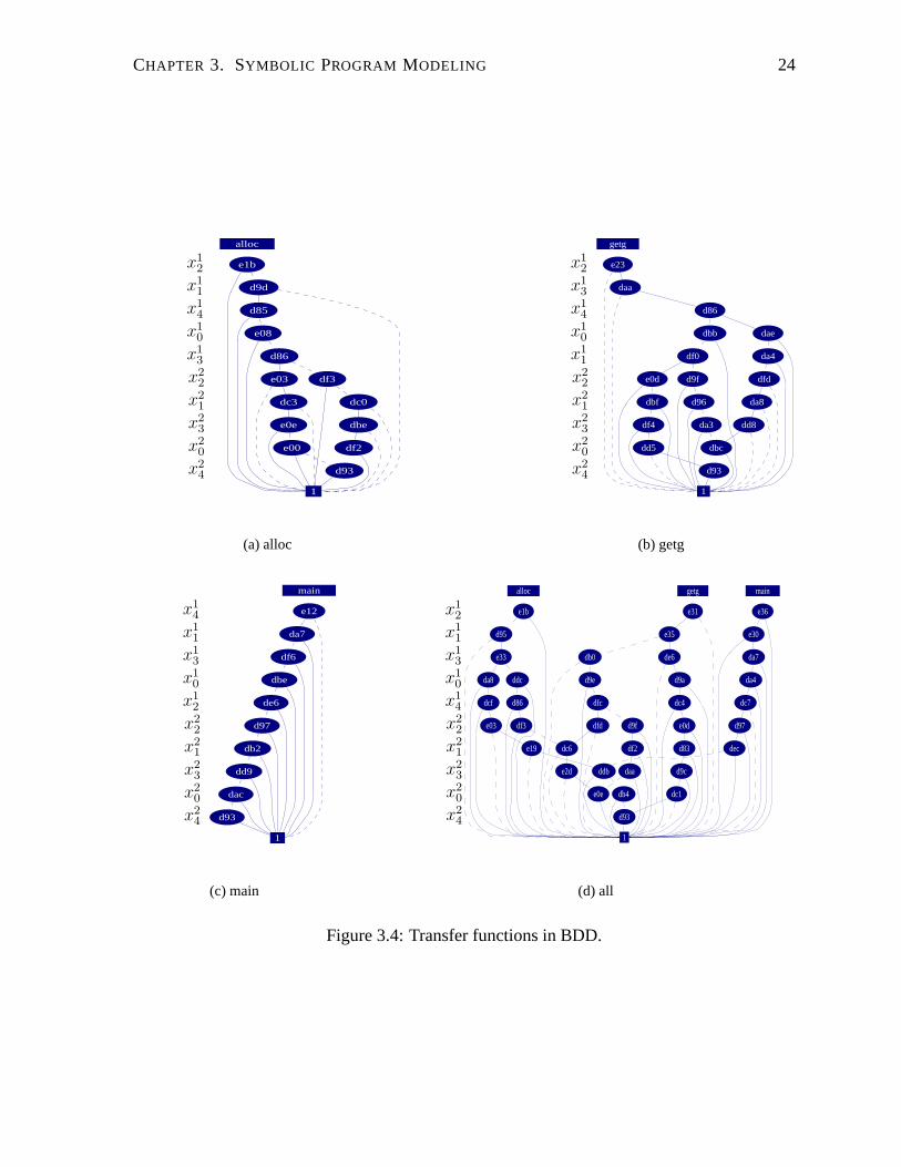
Figure 3.4 shows the BDD representation of symbolic transfer functions in the previous
section. Note that we use BDD to represent both the transfer functions and the program states.
The fact that BDD is nothing but a graph representation of a Boolean function begs the question
that why we do not use the point-to graph in the first place, which seems to be much more
intuitive. One primary advantage of using BDD is that point-to graphs need to be maintained
for every procedure, each of which may share many common edges. In other words, there is
a large amount of redundancy. In contrast, BDD enables the maximum sharing among graph
nodes, and point-to information in different procedures, at different program points can be
reused. As an example, ddb, dc6 are some of the shared internal BDD nodes among different
transfer functions. As the program grows large, such sharing occurs in a large scale. As a
result, when BDD is used to represent a point-to set, its size is not necessarily proportional to
its cardinality, as in the case of point-to graph – often times it is proportional to the dimension
of the Boolean space. This space efficiency will translate into speed efficiency.
CHAPTER 3. SYMBOLIC PROGRAM MODELING 24
alloc
e1b
d9d
1
d85
e08
d86
e03 df3
dc3 dc0
dbee0e
e00 df2
d93
PSfrag replacements
x20
x10
x21
x11
x22
x12
x23
x13
x24
x14
y1
y∗1
y2
y∗2
y3
y∗3
λ0
θ0
λ1
θ1
θ2
λ2
θ3
λ∗0
θ∗0
λ∗1
θ∗1
θ∗2
λ∗2
θ∗3
a
g
r
t
p
q
h1
h2
f
h
m
p1
q1
(a) alloc
getg
e23
daa
1
d86
daedbb
da4df0
d9fe0d dfd
d96 da8dbf
dd8da3df4
dd5 dbc
d93
PSfrag replacements
x20
x10
x21
x11
x22
x12
x23
x13
x24
x14
y1
y∗1
y2
y∗2
y3
y∗3
λ0
θ0
λ1
θ1
θ2
λ2
θ3
λ∗0
θ∗0
λ∗1
θ∗1
θ∗2
λ∗2
θ∗3
a
g
r
t
p
q
h1
h2
f
h
m
p1
q1
(b) getg
main
e12
da7
1
df6
dbe
de6
d97
db2
dd9
dac
d93
PSfrag replacements
x20
x10
x21
x11
x22
x12
x23
x13
x24
x14
y1
y∗1
y2
y∗2
y3
y∗3
λ0
θ0
λ1
θ1
θ2
λ2
θ3
λ∗0
θ∗0
λ∗1
θ∗1
θ∗2
λ∗2
θ∗3
a
g
r
t
p
q
h1
h2
f
h
m
p1
q1
(c) main
alloc getg
e1b
main
e31 e36
e35
1
d95 e30
da7e33 de6db0
da4d9ad9eddcda8
dc4d86 dc7dcf dfc
e03 e0d d97df3 d9fdfd
d83dc6e19 decdf2
e2d ddb d9cdaa
dc1e0e db4
d93
PSfrag replacements
x20
x10
x21
x11
x22
x12
x23
x13
x24
x14
y1
y∗1
y2
y∗2
y3
y∗3
λ0
θ0
λ1
θ1
θ2
λ2
θ3
λ∗0
θ∗0
λ∗1
θ∗1
θ∗2
λ∗2
θ∗3
a
g
r
t
p
q
h1
h2
f
h
m
p1
q1
(d) all
Figure 3.4: Transfer functions in BDD.

CHAPTER 3. SYMBOLIC PROGRAM MODELING 25
3.5 Recurrence Equations
We now describe our pointer analysis framework. In order to focus on the fundamentals,
rather than the implementation details, we assume that after preprocessing, the program can
be characterized by the following mathematical model. In this model, we ignore return values,
as they could be modeled by considering them as parameters to a given procedure. Also note
that for now, we assume the program does not contain indirect calls. As such, the call graph
can be built in advance. From these relations we can calculate the state by applying recurrence
equations.
• I ⊂ [0,∞) is the set of procedures. We also assume that procedure 0 corresponds to the
top procedure in the whole program.
• J ⊂ [0,∞) is the set of memory blocks contained in the program. It includes globals,
locals, parameters and heap objects.
• L ⊂ [0,∞) is the set of program points.
• K ⊂ [0,∞), ∀i ∈ I corresponds to the set of memory dereferences.
• D : K 7→ J × Z characterizes the access path of each memory dereference k ∈ K by a
tuple 〈b, l〉 where b ∈ J is a memory block, and l ∈ Z is the level of dereferences. This
representation can be extended with more complex access patterns.
• {T i(−→λ ,
−→θ )|∀i ∈ I} corresponds to the set of transfer functions for each procedure i.
Here−→λ = [λ0, ...λ|K|−1] corresponds to the initial state blocks, and
−→θ = [θ0, ...θ|K|−1]
corresponds to final state blocks.
• C : I × L 7→ 2I corresponds to the calling relation. For each procedure i ∈ I , and call
site at program point l ∈ L, Ci,l gives the set of callees. C−1i gives the set of tuples 〈j, l〉,
where j ∈ I, l ∈ L, and i ∈ Cj,l.
CHAPTER 3. SYMBOLIC PROGRAM MODELING 26
• B : I × L × K 7→ K is the parameter binding relation. For each call site at program
point l ∈ L, in procedure i ∈ I , and formal parameter dereference k ∈ K at procedure
j ∈ Ci,l, Bi,l,k gives the dereference in procedure i corresponding to the actual.
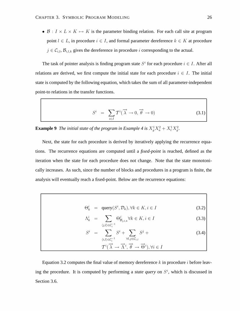
The task of pointer analysis is finding program state S i for each procedure i ∈ I . After all
relations are derived, we first compute the initial state for each procedure i ∈ I . The initial
state is computed by the following equation, which takes the sum of all parameter-independent
point-to relations in the transfer functions.
Si =∑
i∈I
T i(−→λ → 0,
−→θ → 0) (3.1)
Example 9 The initial state of the program in Example 4 is X1gX2
a + X1t X2
g .
Next, the state for each procedure is derived by iteratively applying the recurrence equa-
tions. The recurrence equations are computed until a fixed-point is reached, defined as the
iteration when the state for each procedure does not change. Note that the state monotoni-
cally increases. As such, since the number of blocks and procedures in a program is finite, the
analysis will eventually reach a fixed-point. Below are the recurrence equations:
Θik = query(Si,Dk), ∀k ∈ K, i ∈ I (3.2)
Λik =
∑
〈j,l〉∈C−1
i
ΘjBj,l,k
∀k ∈ K, i ∈ I (3.3)
Si =∑
〈i,l〉∈C−1
i
Si +∑
∀l,j∈Ci,l
Sj + (3.4)
T i(−→λ →
−→Λ i,
−→θ →
−→Θ i), ∀i ∈ I
Equation 3.2 computes the final value of memory dereference k in procedure i before leav-
ing the procedure. It is computed by performing a state query on S i, which is discussed in
Section 3.6.
CHAPTER 3. SYMBOLIC PROGRAM MODELING 27
Equation 3.3 computes the initial value of a formal parameter, denoted by memory deref-
erence k ∈ K, before entering procedure i ∈ I . It is computed by combining the value of
corresponding actuals in all incoming callers. The set of call sites whose callee is this proce-
dure is given by C−1i . Let l ∈ L in procedure j ∈ I be a call site, whose callee is procedure i.
Then, the actual memory dereference corresponding to the formal k is given by Bj,l,k, whose
corresponding value is given by ΘjBj,l,k
.
Lastly, Equation 3.4 computes the state S i by summing the states of its callers and callees as
well as applying the transfer function. Transfer function application is done by substituting the
initial and final state blocks by the actual state blocks computed in Equation 3.3 and Equation
3.2. The transfer function application is discussed in Section 3.7.
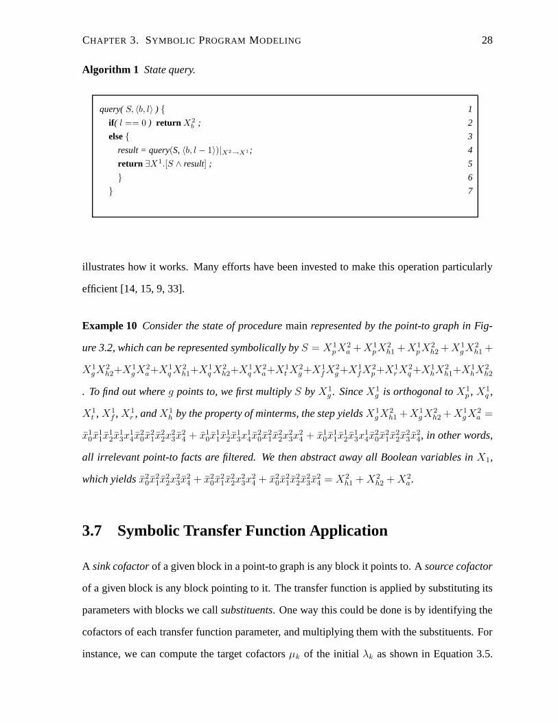
3.6 Symbolic State Query
This section outline the algorithm to perform query on the state of a procedure, also used to
compute Equation 3.2. Given a memory dereference of block b with level l, Algorithm 1 per-
forms the state query by computing the reachable envelope of depth l on the point-to graph
starting from block b. In contrast to the traditional approach where a breadth-first search has to
be performed to explicitly enumerate all neighbors of a node in the point-to graph, our repre-
sentation enables the use of the implicit technique originally developed in the CAD community
for the formal verification of digital hardware. This approach relies on the efficiency of im-
age computation, which collectively computes the set of successors in a graph given a set of
predecessors. Since in our representation, a set of memory blocks can be represented as a dis-
junction of minterms, the query can be formulated as Boolean function manipulation, which
in turn can be efficiently implemented on BDD. As shown in Line 5, the query is performed
by multiplying the state with the minterm of the predecessor using Boolean variables in X 1,
and then existentially abstracting away the Boolean variables in X 1. This procedure is per-
formed recursively, by applying the mirror operation on Line 4 to previous results. Example 10
CHAPTER 3. SYMBOLIC PROGRAM MODELING 28
Algorithm 1 State query.
query( S, 〈b, l〉 ) { 1
if( l == 0 ) return X2b ; 2
else { 3
result = query(S, 〈b, l − 1〉)|X2→X1; 4
return ∃X1.[S ∧ result] ; 5
} 6
} 7
illustrates how it works. Many efforts have been invested to make this operation particularly
efficient [14, 15, 9, 33].
Example 10 Consider the state of procedure main represented by the point-to graph in Fig-
ure 3.2, which can be represented symbolically by S = X 1pX2
a + X1pX2
h1 + X1pX2
h2 + X1g X2
h1 +
X1gX2
h2+X1gX2
a+X1q X2
h1+X1q X2
h2+X1q X2
a+X1t X2
g +X1fX2
g +X1fX2
p+X1r X2
q +X1hX2
h1+X1hX2
h2
. To find out where g points to, we first multiply S by X1g . Since X1
g is orthogonal to X1p , X1
q ,
X1t , X1
f , X1r , and X1
h by the property of minterms, the step yields X1gX2
h1 + X1g X2
h2 + X1gX2
a =
x10x
11x
12x
13x
14x
20x
21x
22x
23x
24 + x1
0x11x
12x
13x
14x
20x
21x
22x
23x
24 + x1
0x11x
12x
13x
14x
20x
21x
22x
23x
24, in other words,
all irrelevant point-to facts are filtered. We then abstract away all Boolean variables in X1,
which yields x20x
21x
22x
23x
24 + x2
0x21x
22x
23x
24 + x2
0x21x
22x
23x
24 = X2
h1 + X2h2 + X2
a .
3.7 Symbolic Transfer Function Application
A sink cofactor of a given block in a point-to graph is any block it points to. A source cofactor
of a given block is any block pointing to it. The transfer function is applied by substituting its
parameters with blocks we call substituents. One way this could be done is by identifying the
cofactors of each transfer function parameter, and multiplying them with the substituents. For
instance, we can compute the target cofactors µk of the initial λk as shown in Equation 3.5.

CHAPTER 3. SYMBOLIC PROGRAM MODELING 29
Similar to the query computation, to find µk we multiply T i by X2λk
, and then abstract away
the Boolean variables in X2. The state is then updated with the new point-to relation as shown
in Equation 3.6. The main disadvantage of this approach is that we must identify the cofactors
of each parameter, and then multiply them by the substituents ( Λik in this case ) separately.
µk = ∃X2.(X2λk
· T i) (3.5)
Si = Si + (µk · Λik) (3.6)
We propose a new method such that the substitutions can be performed collectively. First,
to represent the relation B × B between the pointers and their values we introduce two ad-
ditional Boolean variable sets Y 1 and Y 2 respectively. We can derive minterms using these
two Boolean variable sets in the same manner they were derived using X 1 and X2. To be
able to substitute collectively, we modify each of the transfer functions T i into an augmented
transfer function T i. We derive T i by multiplying each transfer function parameter minterm
using Boolean variables in X1 by the corresponding minterm using Boolean variables in Y 1.
Likewise, we multiply each transfer function parameter minterm using Boolean variables in
X2 by the corresponding minterm using Boolean variables in Y 2. We then abstract away the
transfer function parameter minterms using Boolean variables in X 1 and X2.
Example 11 The augmented transfer functions of procedures in Example 4 are: T alloc =
X1fY 2
λ0+ X1
hY 2λ1
+ Y 1θ0
Y 2θ1
, T getg = X1r Y 2
λ2+ X1
t X2g + Y 1
θ2Y 2
θ3, and T main = T main.
Now, we can create a binding between all substituents and parameters. The determinant of a
substituent minterm encoded using Boolean variables in X 1 and X2 is the matching parameter
minterm in domains Y 1 and Y 2 respectively. We can derive the binding by multiplying each
substituent minterm by its determinant. As shown in Algorithm 2, the binding can be used to
multiply the augmented transfer function. Note that terms with different determinants will be
canceled thanks to the orthogonality of minterms. Hence, the substitution can be performed by
a single multiplication followed by existentially abstracting away the determinant variables.

CHAPTER 3. SYMBOLIC PROGRAM MODELING 30
Algorithm 2 Transfer Function Application.
apply( T i,−→Λ i,
−→Θ i ) { 8
binding =∑
k∈K(Y 2λk
Λik + Y 2
θkΘi
k); 9
s = ∃Y 2.[T i ∧ binding]; 10
binding∗ = binding|X2→X1,Y 2→Y 1; 11
return ∃Y 1.[s ∧ binding∗] ; 12
} 13

Chapter 4
Symbolic Context-Sensitive Analysis
In this chapter we describe the context-sensitive analysis. In Section 4.1 we introduce the
symbolic invocation graph. In Section 4.2 we show how the acyclic call graph is derived.
In Section 4.3 we explain how the acyclic call graph is used in constructing the symbolic
invocation graph, and discuss the complexity. In Section 4.4 we describe how the symbolic
invocation graph can be leveraged in order to perform the context-sensitive analysis.
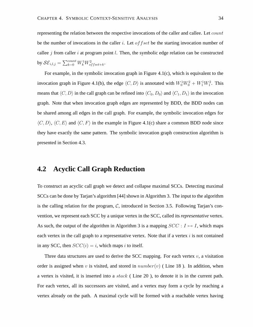
4.1 Invocation Graph
An invocation of a procedure corresponds to one of the calling contexts of the procedure, and
can be characterized by a distinct number. An invocation graph is the expansion of the call
graph [17] whose vertices correspond to the invocations of procedures. Figure 4.1(a) shows
the call graph of a program, where the edges are labeled with the respective call sites. The
corresponding invocation graph is shown in Figure 4.1(b), where each vertex is labeled by the
procedure name and an integer index representing the different invocations of each procedure.
The goal of the context-sensitive analysis is to distinguish between the state of each invo-
cation of a procedure. Since the pointer analysis is flow-insensitive, the point-to relations for
globals and heap locations are propagated to all invocations in the program. Hence, the main
advantage of the context-sensitive analysis is the ability to distinguish between the values of
31

CHAPTER 4. SYMBOLIC CONTEXT-SENSITIVE ANALYSIS 32
12
1
12
3
PSfrag replacements
x20
x10
x21
x11
x22
x12
x23
x13
x24
x14
y1
y∗1
y2
y∗2
y3
y∗3
λ0
θ0
λ1
θ1
θ2
λ2
θ3
λ∗0
θ∗0
λ∗1
θ∗1
θ∗2
λ∗2
θ∗3
a
g
r
t
p
q
h1
h2
f
h
m
p1
q1
A
B
C
D E F
A0
B0
C0
D0
E0
F0
C1
D1
E1
F1
(a) Call Graph
2 1
12 3
1
1 2 3
PSfrag replacements
x20
x10
x21
x11
x22
x12
x23
x13
x24
x14
y1
y∗1
y2
y∗2
y3
y∗3
λ0
θ0
λ1
θ1
θ2
λ2
θ3
λ∗0
θ∗0
λ∗1
θ∗1
θ∗2
λ∗2
θ∗3
a
g
r
t
p
q
h1
h2
f
h
m
p1
q1
A
B
C
D
E
F
A0
B0
C0
D0 E0 F0
C1
D1 E1 F1
(b) Invocation Graph
12
1
12
3
PSfrag replacements
x20
x10
x21
x11
x22
x12
x23
x13
x24
x14
y1
y∗1
y2
y∗2
y3
y∗3
λ0
θ0
λ1
θ1
θ2
λ2
θ3
λ∗0
θ∗0
λ∗1
θ∗1
θ∗2
λ∗2
θ∗3
a
g
r
t
p
q
h1
h2
f
h
m
p1
q1
A
B
C
D E F
A0
B0
C0
D0
E0
F0
C1
D1
E1
F1
W 00 W 1
0
W 00 W 1
0
W 00 W 1
1
W 01 W 1
0
W 01 W 1
1W 0
0 W 10 +
W 01 W 1
1
W 00 W 1
0 +
W 01 W 1
1
W 00 W 1
0 +
W 01 W 1
1
(c) Symbolic Invocation Graph
Figure 4.1: A Call Graph and Invocation Graph

CHAPTER 4. SYMBOLIC CONTEXT-SENSITIVE ANALYSIS 33
parameters, for different invocations of the same procedure.
Note that cycles in the call graph pose a problem in deriving the invocation graph. The
cycles are caused by recursive calls between procedures. Naively expanding the call graph
may result in an invocation graph of infinite size. This is because each vertex on a cycle in
the call graph may have to be expanded indefinitely. As such, cycles in the call graph must be
handled in advance. A strongly connected component is a subgraph where each vertex in the
component is reachable from another vertex in the component. A maximal SCC is a SCC not
contained in any other SCCs. By collapsing maximal SCCs into a single vertex, we can obtain
an acyclic call graph. By doing so, an acyclic call graph is derived, and new invocations are
allocated for each each incoming edge into the maximal SCC. The derivation of the acyclic
graph, and the resulting invocation graph will be elaborated Section 4.2.
With an acyclic call graph, multiple paths can be expanded, visiting each vertex only once
in a topological pass over the acyclic call graph. However, the invocation graph is exponential
in relation to the call graph, and hence the cost of constructing the vertices and edges of the
invocation graph is exponential. To resolve this issue, note that edges in the invocation graph
can be characterized by a relation between the invocations of the caller and callee in the call
graph. Thus, instead of expanding call graph edges we could annotate them with the relation
between the invocations of the caller and callee. Such annotation could be a Boolean func-
tion, representing the relation between the invocations of the caller and callee with two sets of
Boolean variables, W 1 and W 2 respectively. We can derive the minterm for the invocation of
a procedure, using the invocation number binary representation, and the Boolean variables in
either W 1 or W 2. For example, C0 in Figure 4.1(b) can be identified by C and the minterm
W 10 .
We define a symbolic invocation graph to be an annotation of the call graph C, where
each edge 〈i, l, j〉 ∈ C, corresponding to a call at program point l in procedure i, to procedure
j, is annotated with a Boolean function SE i,l,j, referred to as the symbolic edge relation. The
symbolic edge relation replaces the set of invocation graph edges associated with a call site by
CHAPTER 4. SYMBOLIC CONTEXT-SENSITIVE ANALYSIS 34
representing the relation between the respective invocations of the caller and callee. Let count
be the number of invocations in the caller i. Let offset be the starting invocation number of
callee j from caller i at program point l. Then, the symbolic edge relation can be constructed
by SE i,l,j =∑count
k=0 W 1k W 2
offset+k.
For example, in the symbolic invocation graph in Figure 4.1(c), which is equivalent to the
invocation graph in Figure 4.1(b), the edge 〈C, D〉 is annotated with W 10 W 2
0 + W 11 W 2
1 . This
means that 〈C, D〉 in the call graph can be refined into 〈C0, D0〉 and 〈C1, D1〉 in the invocation
graph. Note that when invocation graph edges are represented by BDD, the BDD nodes can
be shared among all edges in the call graph. For example, the symbolic invocation edges for
〈C, D〉, 〈C, E〉 and 〈C, F 〉 in the example in Figure 4.1(c) share a common BDD node since
they have exactly the same pattern. The symbolic invocation graph construction algorithm is
presented in Section 4.3.
4.2 Acyclic Call Graph Reduction
To construct an acyclic call graph we detect and collapse maximal SCCs. Detecting maximal
SCCs can be done by Tarjan’s algorithm [44] shown in Algorithm 3. The input to the algorithm
is the calling relation for the program, C, introduced in Section 3.5. Following Tarjan’s con-
vention, we represent each SCC by a unique vertex in the SCC, called its representative vertex.
As such, the output of the algorithm in Algorithm 3 is a mapping SCC : I 7→ I , which maps
each vertex in the call graph to a representative vertex. Note that if a vertex i is not contained
in any SCC, then SCC(i) = i, which maps i to itself.
Three data structures are used to derive the SCC mapping. For each vertex v, a visitation
order is assigned when v is visited, and stored in number(v) ( Line 18 ). In addition, when
a vertex is visited, it is inserted into a stack ( Line 20 ), to denote it is in the current path.
For each vertex, all its successors are visited, and a vertex may form a cycle by reaching a
vertex already on the path. A maximal cycle will be formed with a reachable vertex having
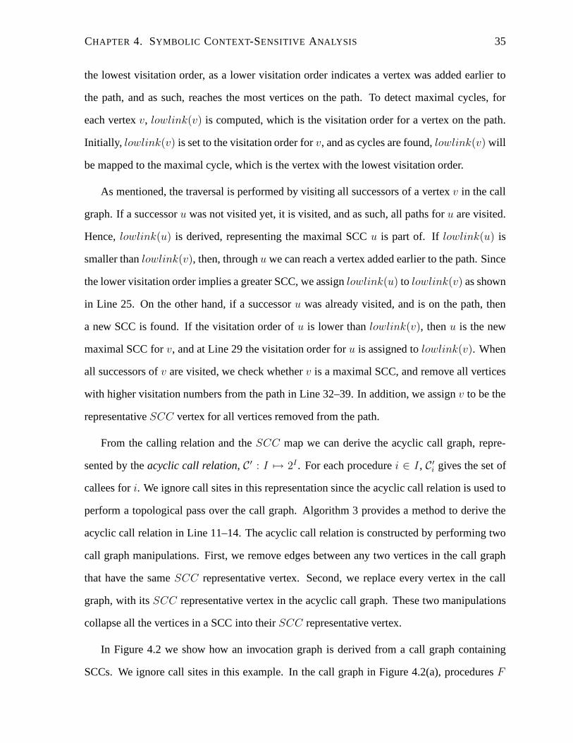
CHAPTER 4. SYMBOLIC CONTEXT-SENSITIVE ANALYSIS 35
the lowest visitation order, as a lower visitation order indicates a vertex was added earlier to
the path, and as such, reaches the most vertices on the path. To detect maximal cycles, for
each vertex v, lowlink(v) is computed, which is the visitation order for a vertex on the path.
Initially, lowlink(v) is set to the visitation order for v, and as cycles are found, lowlink(v) will
be mapped to the maximal cycle, which is the vertex with the lowest visitation order.
As mentioned, the traversal is performed by visiting all successors of a vertex v in the call
graph. If a successor u was not visited yet, it is visited, and as such, all paths for u are visited.
Hence, lowlink(u) is derived, representing the maximal SCC u is part of. If lowlink(u) is
smaller than lowlink(v), then, through u we can reach a vertex added earlier to the path. Since
the lower visitation order implies a greater SCC, we assign lowlink(u) to lowlink(v) as shown
in Line 25. On the other hand, if a successor u was already visited, and is on the path, then
a new SCC is found. If the visitation order of u is lower than lowlink(v), then u is the new
maximal SCC for v, and at Line 29 the visitation order for u is assigned to lowlink(v). When
all successors of v are visited, we check whether v is a maximal SCC, and remove all vertices
with higher visitation numbers from the path in Line 32–39. In addition, we assign v to be the
representative SCC vertex for all vertices removed from the path.
From the calling relation and the SCC map we can derive the acyclic call graph, repre-
sented by the acyclic call relation, C ′ : I 7→ 2I . For each procedure i ∈ I , C ′i gives the set of
callees for i. We ignore call sites in this representation since the acyclic call relation is used to
perform a topological pass over the call graph. Algorithm 3 provides a method to derive the
acyclic call relation in Line 11–14. The acyclic call relation is constructed by performing two
call graph manipulations. First, we remove edges between any two vertices in the call graph
that have the same SCC representative vertex. Second, we replace every vertex in the call
graph, with its SCC representative vertex in the acyclic call graph. These two manipulations
collapse all the vertices in a SCC into their SCC representative vertex.
In Figure 4.2 we show how an invocation graph is derived from a call graph containing
SCCs. We ignore call sites in this example. In the call graph in Figure 4.2(a), procedures F

CHAPTER 4. SYMBOLIC CONTEXT-SENSITIVE ANALYSIS 36
Algorithm 3 Maximal SCC detection based on Tarjan’s Algorithm
var number, lowlink : I 7→ Z; 1
var stack : Z 7→ I; var sp : Z; 2
var SCC : I 7→ I; 3
var visitOrder : Z; 4
5
acyclicReduction( ) { 6
sccNum = sp = 0; 7
forall( i ∈ I ) lowlink(v) = number(v) = 0; 8
identifyScc(0); 9
10
forall( i ∈ I ) C′
i = �; 11
forall( 〈i, l, j〉 ∈ Ci,l ) 12
if( SCC(i) 6= SCC(j) ) 13
C′ = C′ ∪ 〈SCC(i), SCC(j)〉; 14
} 15
16
identifyScc( v ) { 17
number(v) = ++sccNum; 18
lowlink(v) = number(v); 19
stack(sp++) = v; 20
21
forall( 〈i, l, j〉 ∈ C ) { 22
if( number(w) == 0 ) { 23
identifyScc(w); 24
lowlink(v) = min(lowlink(v), lowlink(w)); 25
} 26
else if( number(w) < number(v) ) 27
if( ∃k stack(k) == w ) 28
lowlink(v) = min(lowlink(v), number(w)); 29
} 30
31
if( lowlink(v) == number(v) ) { 32
w = stack(sp); 33
while( number(w) ≥ number(v) ) { 34
sp = sp - 1; 35
SCC(w) = v; 36
w = stack(sp); 37
} 38
} 39
} 40
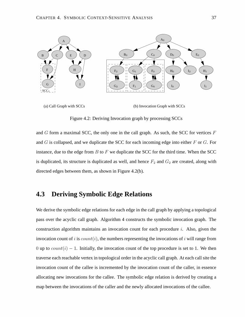
CHAPTER 4. SYMBOLIC CONTEXT-SENSITIVE ANALYSIS 37
PSfrag replacements
x20
x10
x21
x11
x22
x12
x23
x13
x24
x14
y1
y∗1
y2
y∗2
y3
y∗3
λ0
θ0
λ1
θ1
θ2
λ2
θ3
λ∗0
θ∗0
λ∗1
θ∗1
θ∗2
λ∗2
θ∗3
a
g
r
t
p
q
h1
h2
f
h
m
p1
q1
A
B C DE
F
A0
B0
C0
D0
E0
F0
C1
D1
E1
F1
G
H
I
F0
F1
F2
G0
G1
G2
G0
H0
H1
I0
I1
I2
SCC1
(a) Call Graph with SCCs
PSfrag replacements
x20
x10
x21
x11
x22
x12
x23
x13
x24
x14
y1
y∗1
y2
y∗2
y3
y∗3
λ0
θ0
λ1
θ1
θ2
λ2
θ3
λ∗0
θ∗0
λ∗1
θ∗1
θ∗2
λ∗2
θ∗3
a
g
r
t
p
q
h1
h2
f
h
m
p1
q1
A
B
C
D
E
F
A0
B0 C0 D0 E0
F0
C1
D1
E1
F1
G
H
I
F0
F1
F2
G0
G1
G2 G0
H0 H1
I0 I1
I2
SCC1
(b) Invocation Graph with SCCs
Figure 4.2: Deriving Invocation graph by processing SCCs
and G form a maximal SCC, the only one in the call graph. As such, the SCC for vertices F
and G is collapsed, and we duplicate the SCC for each incoming edge into either F or G. For
instance, due to the edge from B to F we duplicate the SCC for the third time. When the SCC
is duplicated, its structure is duplicated as well, and hence F2 and G2 are created, along with
directed edges between them, as shown in Figure 4.2(b).
4.3 Deriving Symbolic Edge Relations
We derive the symbolic edge relations for each edge in the call graph by applying a topological
pass over the acyclic call graph. Algorithm 4 constructs the symbolic invocation graph. The
construction algorithm maintains an invocation count for each procedure i. Also, given the
invocation count of i is count(i), the numbers representing the invocations of i will range from
0 up to count(i) − 1. Initially, the invocation count of the top procedure is set to 1. We then
traverse each reachable vertex in topological order in the acyclic call graph. At each call site the
invocation count of the callee is incremented by the invocation count of the caller, in essence
allocating new invocations for the callee. The symbolic edge relation is derived by creating a
map between the invocations of the caller and the newly allocated invocations of the callee.
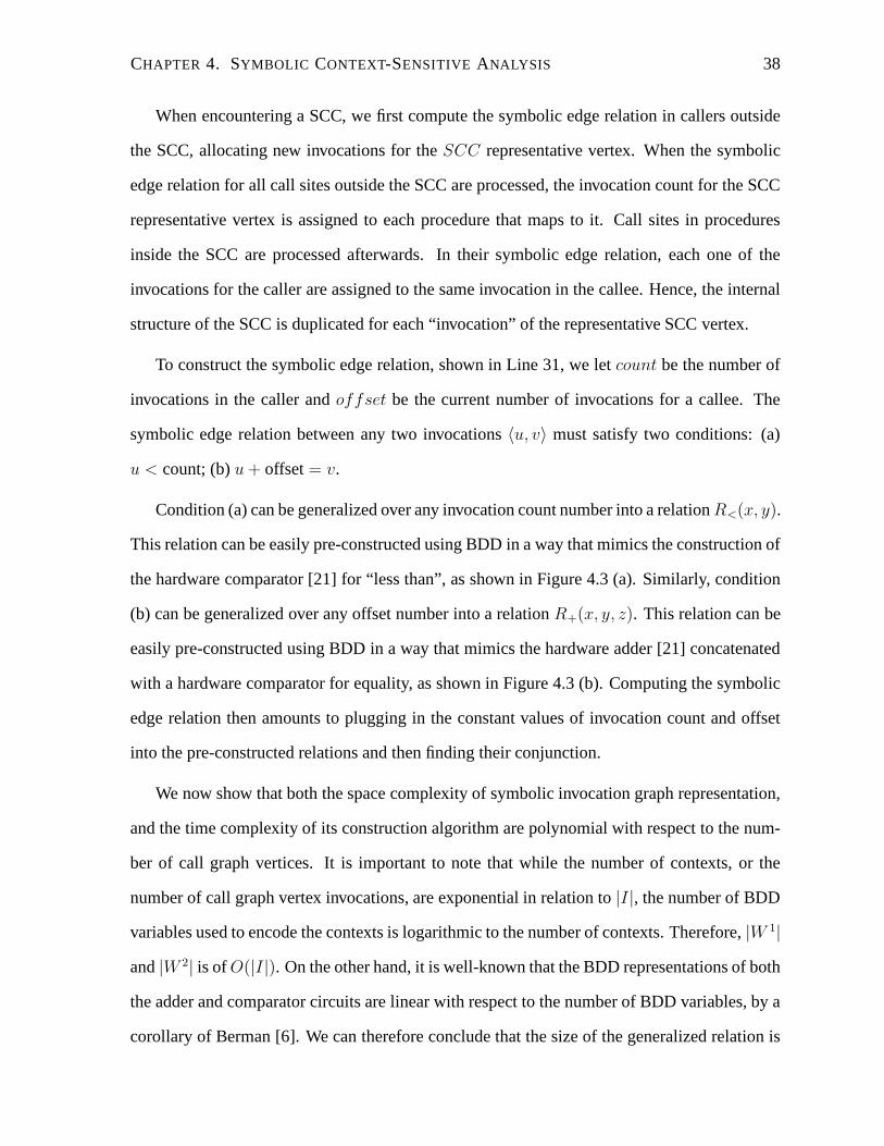
CHAPTER 4. SYMBOLIC CONTEXT-SENSITIVE ANALYSIS 38
When encountering a SCC, we first compute the symbolic edge relation in callers outside
the SCC, allocating new invocations for the SCC representative vertex. When the symbolic
edge relation for all call sites outside the SCC are processed, the invocation count for the SCC
representative vertex is assigned to each procedure that maps to it. Call sites in procedures
inside the SCC are processed afterwards. In their symbolic edge relation, each one of the
invocations for the caller are assigned to the same invocation in the callee. Hence, the internal
structure of the SCC is duplicated for each “invocation” of the representative SCC vertex.
To construct the symbolic edge relation, shown in Line 31, we let count be the number of
invocations in the caller and offset be the current number of invocations for a callee. The
symbolic edge relation between any two invocations 〈u, v〉 must satisfy two conditions: (a)
u < count; (b) u + offset = v.
Condition (a) can be generalized over any invocation count number into a relation R<(x, y).
This relation can be easily pre-constructed using BDD in a way that mimics the construction of
the hardware comparator [21] for “less than”, as shown in Figure 4.3 (a). Similarly, condition
(b) can be generalized over any offset number into a relation R+(x, y, z). This relation can be
easily pre-constructed using BDD in a way that mimics the hardware adder [21] concatenated
with a hardware comparator for equality, as shown in Figure 4.3 (b). Computing the symbolic
edge relation then amounts to plugging in the constant values of invocation count and offset
into the pre-constructed relations and then finding their conjunction.
We now show that both the space complexity of symbolic invocation graph representation,
and the time complexity of its construction algorithm are polynomial with respect to the num-
ber of call graph vertices. It is important to note that while the number of contexts, or the
number of call graph vertex invocations, are exponential in relation to |I|, the number of BDD
variables used to encode the contexts is logarithmic to the number of contexts. Therefore, |W 1|
and |W 2| is of O(|I|). On the other hand, it is well-known that the BDD representations of both
the adder and comparator circuits are linear with respect to the number of BDD variables, by a
corollary of Berman [6]. We can therefore conclude that the size of the generalized relation is
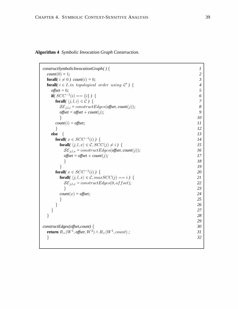
CHAPTER 4. SYMBOLIC CONTEXT-SENSITIVE ANALYSIS 39
Algorithm 4 Symbolic Invocation Graph Construction.
constructSymbolicInvocationGraph( ) { 1count(0) = 1; 2forall( i 6= 0 ) count(i) = 0; 3forall( i ∈ I, in topological order using C ′ ) { 4
offset = 0; 5if( SCC−1(i) == {i} ) { 6
forall( 〈j, l, i〉 ∈ C ) { 7SEj,l,i = constructEdges(offset, count(j)); 8offset = offset + count(j); 9} 10
count(i) = offset; 11} 12
else { 13forall( x ∈ SCC−1(i) ) { 14
forall( 〈j, l, x〉 ∈ C, SCC(j) 6= i ) { 15SEj,l,x = constructEdges(offset, count(j)); 16offset = offset + count(j); 17} 18
} 19forall( x ∈ SCC−1(i) ) { 20
forall( 〈j, l, x〉 ∈ C,maxSCC(j) == i ) { 21SEj,l,x = constructEdges(0, offset); 22} 23
count(x) = offset; 24} 25
} 26} 27
} 2829
constructEdges(offset,count) { 30return R+(W 1, offset,W 2) ∧ R<(W 1, count) ; 31} 32

CHAPTER 4. SYMBOLIC CONTEXT-SENSITIVE ANALYSIS 40
PSfrag replacements
x20
x10
x21
x11
x22
x12
x23
x13
x24
x14
y1
y∗1
y2
y∗2
y3
y∗3
λ0
θ0
λ1
θ1
θ2
λ2
θ3
λ∗0
θ∗0
λ∗1
θ∗1
θ∗2
λ∗2
θ∗3
a
g
r
t
p
q
h1
h2
f
h
m
p1
q1
A
B
C
D
E
F
A0
B0
C0
D0
E0
F0
C1
D1
E1
F1
x0 y0
z0
x1 y1
z1
x2 y2
z2
x3 y3
z3
x0y0z0
x1y1z1
x2y2z2
x3y3z3
y0
z0
x1
y1
z1
x2
y2
z2
x3
y3
z3
0
(a) R<(x, y) : x < y
PSfrag replacements
x20
x10
x21
x11
x22
x12
x23
x13
x24
x14
y1
y∗1
y2
y∗2
y3
y∗3
λ0
θ0
λ1
θ1
θ2
λ2
θ3
λ∗0
θ∗0
λ∗1
θ∗1
θ∗2
λ∗2
θ∗3
a
g
r
t
p
q
h1
h2
f
h
m
p1
q1
A
B
C
D
E
F
A0
B0
C0
D0
E0
F0
C1
D1
E1
F1
x0
y0
z0
x1
y1
z1
x2
y2
z2
x3
y3
z3
x0y0z0 x1y1z1 x2y2z2 x3y3z3
y0
z0
x1
y1
z1
x2
y2
z2
x3
y3
z3
0
(b) R+(x, y, z) : x + y = z
Figure 4.3: Construction of helper symbolic relations.
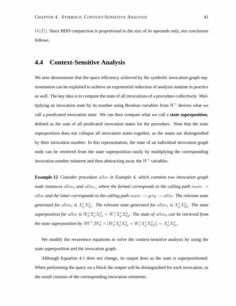
CHAPTER 4. SYMBOLIC CONTEXT-SENSITIVE ANALYSIS 41
O(|I|). Since BDD conjunction is proportional to the size of its operands only, our conclusion
follows.
4.4 Context-Sensitive Analysis
We now demonstrate that the space efficiency achieved by the symbolic invocation graph rep-
resentation can be exploited to achieve an exponential reduction of analysis runtime in practice
as well. The key idea is to compute the state of all invocations of a procedure collectively. Mul-
tiplying an invocation state by its number using Boolean variables from W 1 derives what we
call a predicated invocation state. We can then compute what we call a state superposition,
defined as the sum of all predicated invocation states for the procedure. Note that the state
superposition does not collapse all invocation states together, as the states are distinguished
by their invocation number. In this representation, the state of an individual invocation graph
node can be retrieved from the state superposition easily by multiplying the corresponding
invocation number minterm and then abstracting away the W 1 variables.
Example 12 Consider procedure alloc in Example 4, which contains two invocation graph
node instances alloc0 and alloc1, where the formal corresponds to the calling path main →
alloc and the latter corresponds to the calling path main → getg → alloc. The relevant state
generated for alloc0 is X1pX2
h1. The relevant state generated for alloc1 is X1gX2
h2. The state
superposition for alloc is W 10 X1
pX2h1 + W 1
1 X1gX2
h2. The state of alloc0 can be retrieved from
the state superposition by ∃W 1.[W 10 ∧ (W 1
0 X1pX2
h1 + W 11 X1
gX2h2)] = X1
pX2h1.
We modify the recurrence equations to solve the context-sensitive analysis by using the
state superposition and the invocation graph.
Although Equation 4.1 does not change, its output does as the state is superpositioned.
When performing the query on a block the output will be distinguished for each invocation, as
the result consists of the corresponding invocation minterms.
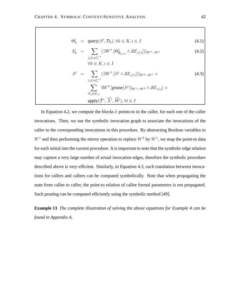
CHAPTER 4. SYMBOLIC CONTEXT-SENSITIVE ANALYSIS 42
Θik = query(Si,Dk), ∀k ∈ K, i ∈ I (4.1)
Λik =
∑
〈j,l〉∈C−1
i
(∃W 1.[ΘjBj,l,k
∧ SE j,l,i])|W 2→W 1 (4.2)
∀k ∈ K, i ∈ I
Si =∑
〈j,l〉∈C−1
i
(∃W 1.[Sj ∧ SE j,l,i])|W 2→W 1 + (4.3)
∑
∀l,j∈Ci,l
∃W 2.[prune(Sj)|W 1→W 2 ∧ SE i,l,j] +
apply(T i,−→Λ i,
−→Θ i), ∀i ∈ I
In Equation 4.2, we compute the blocks k points-to in the caller, for each one of the caller
invocations. Then, we use the symbolic invocation graph to associate the invocations of the
caller to the corresponding invocations in this procedure. By abstracting Boolean variables in
W 1 and then performing the mirror operation to replace W 2 by W 1, we map the point-to data
for each initial into the current procedure. It is important to note that the symbolic edge relation
may capture a very large number of actual invocation edges, therefore the symbolic procedure
described above is very efficient. Similarly, in Equation 4.3, such translation between invoca-
tions for callers and callees can be computed symbolically. Note that when propagating the
state from callee to caller, the point-to relation of callee formal parameters is not propagated.
Such pruning can be computed efficiently using the symbolic method [49].
Example 13 The complete illustration of solving the above equations for Example 4 can be
found in Appendix A.

Chapter 5
Experimental Results
Our symbolic pointer analysis tool is implemented in C, and makes use of a compiler infras-
tructure to translate from several frontends (e.g. C, Java, Verilog, etc.), into an intermediate
representation (IR). In the setup pass, the infrastructure traverses the IR generated by the fron-
tends to produce the call graph (CG). Following the setup, an intraprocedural analysis pass
is performed on all user-defined procedures in the program, iterating over the instructions and
creating the transfer function for each procedure. An interprocedural pass is then applied,
which performs either a context-insensitive analysis, or context-sensitive analysis. We use
Somenzi’s publicly available CUDD package [42] for BDD implementation. Our current im-
plementation does not support non-local control transfer (setjmp/longjmp calls), location sets
[48], and assumes no ill advised use of pointers is made (like random memory accessing via
integers). Heap objects are named after the allocation site. Lastly, the C library function’s
transfer functions are precomputed and applied as necessary.
The goal of our empirical evaluation is three-fold. Our primary goal is to quantify the
speed and space efficiency of the proposed symbolic method which is shown in Section 5.1
and Section 5.2. Our second goal is to verify the context-sensitive analysis is more precise than
the context-insensitive analysis, and the results are presented and discussed in Section 5.3. Our
third goal is to quantify various BDD-related engineering issues. In Section 5.4 we evaluate
43
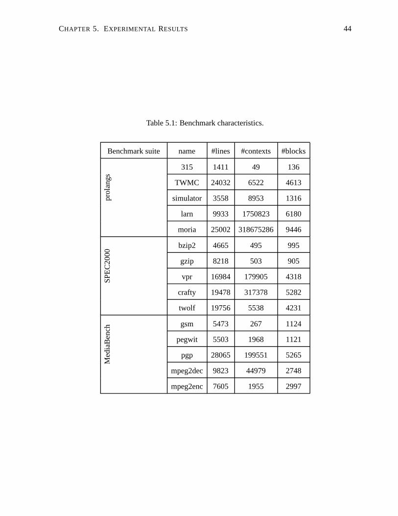
CHAPTER 5. EXPERIMENTAL RESULTS 44
Table 5.1: Benchmark characteristics.
Benchmark suite name #lines #contexts #blocks
prol
angs
315 1411 49 136
TWMC 24032 6522 4613
simulator 3558 8953 1316
larn 9933 1750823 6180
moria 25002 318675286 9446
SPE
C20
00
bzip2 4665 495 995
gzip 8218 503 905
vpr 16984 179905 4318
crafty 19478 317378 5282
twolf 19756 5538 4231
Med
iaB
ench
gsm 5473 267 1124
pegwit 5503 1968 1121
pgp 28065 199551 5265
mpeg2dec 9823 44979 2748
mpeg2enc 7605 1955 2997
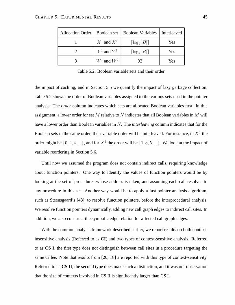
CHAPTER 5. EXPERIMENTAL RESULTS 45
Allocation Order Boolean set Boolean Variables Interleaved
1 X1 and X2 dlog2 |B|e Yes
2 Y 1 and Y 2 dlog2 |B|e Yes
3 W 1 and W 2 32 Yes
Table 5.2: Boolean variable sets and their order
the impact of caching, and in Section 5.5 we quantify the impact of lazy garbage collection.
Table 5.2 shows the order of Boolean variables assigned to the various sets used in the pointer
analysis. The order column indicates which sets are allocated Boolean variables first. In this
assignment, a lower order for set M relative to N indicates that all Boolean variables in M will
have a lower order than Boolean variables in N . The interleaving column indicates that for the
Boolean sets in the same order, their variable order will be interleaved. For instance, in X 1 the
order might be {0, 2, 4, ...}, and for X2 the order will be {1, 3, 5, ...}. We look at the impact of
variable reordering in Section 5.6.
Until now we assumed the program does not contain indirect calls, requiring knowledge
about function pointers. One way to identify the values of function pointers would be by
looking at the set of procedures whose address is taken, and assuming each call resolves to
any procedure in this set. Another way would be to apply a fast pointer analysis algorithm,
such as Steensgaard’s [43], to resolve function pointers, before the interprocedural analysis.
We resolve function pointers dynamically, adding new call graph edges to indirect call sites. In
addition, we also construct the symbolic edge relation for affected call graph edges.
With the common analysis framework described earlier, we report results on both context-
insensitive analysis (Referred to as CI) and two types of context-sensitive analysis. Referred
to as CS I, the first type does not distinguish between call sites in a procedure targeting the
same callee. Note that results from [20, 18] are reported with this type of context-sensitivity.
Referred to as CS II, the second type does make such a distinction, and it was our observation
that the size of contexts involved in CS II is significantly larger than CS I.
CHAPTER 5. EXPERIMENTAL RESULTS 46
We perform our evaluation against three benchmark suites: prolangs [37], the popular
benchmark suite from the pointer analysis community, the integer suite in SPEC2000 [1], and
finally MediaBench [29]. The prolangs benchmarks were utilized in evaluating the perfor-
mance of many pointer analysis algorithms, and as such serves as a valid comparison with
previous work in this area. The SPEC2000 and MediaBench benchmarks, which are relatively
large, are selected to help study the robustness and scalability of our algorithm. The character-
istics of the reported benchmarks in this paper are shown in Table 5.1.
The experiment was performed on a Sun Blade 150 workstation with 550 MHz CPU and
128MB RAM, running on Solaris 8 Operating System. The executable was built using gcc-2.93
with the -O2 option.
5.1 Space Efficiency
In Table 5.3 we show the memory consumption of the BDD manager for each benchmark.
As it can be seen, the total memory usage never exceeds 11MB. In Figure 5.1, we present a
different point of view on the memory consumption of the context-sensitive pointer analysis.
The horizontal axis shows the number of contexts in the evaluated benchmarks, which is the
number of invocation graph nodes, if an explicit invocation graph representation is used, in log
scale. The vertical axis on the right hand side corresponds to the number of BDD nodes used to
represent the symbolic invocation graph, and the left vertical axis corresponds to the memory
consumption of the BDD manager.
As it can be seen, the memory consumption does not explode as the number of contexts
significantly increases. The memory consumption is roughly around 10 MB for most bench-
marks. A key reason for the relatively low memory consumption is the symbolic invocation
graph, and its space efficiency. From Figure 5.1, the number of BDD nodes required to rep-
resent the symbolic invocation graph mostly increases with context count, and never exceeds
60,000; for a benchmark with half a billion contexts. From Figure 5.1, it can be seen that

CHAPTER 5. EXPERIMENTAL RESULTS 47
1
2
3
4
5
6
7
8
9
10
11
12
To
tal S
pac
e (
MB
)
Contexts101 102 103 104 105 106 107 108 109 0
1
2
3
4
5
6
7
8
9
10
11
12
x 104
# B
DD
No
des
in S
ymb
olic
Invo
cati
on
Gra
ph
Total SpaceNumber of BDD Nodes
PSfrag replacements
x20
x10
x21
x11
x22
x12
x23
x13
x24
x14
y1
y∗1
y2
y∗2
y3
y∗3
λ0
θ0
λ1
θ1
θ2
λ2
θ3
λ∗0
θ∗0
λ∗1
θ∗1
θ∗2
λ∗2
θ∗3
a
g
r
t
p
q
h1
h2
f
h
m
p1
q1
A
B
C
D
E
F
A0
B0
C0
D0
E0
F0
C1
D1
E1
F1
Figure 5.1: Memory usage versus context count.
compared to the corresponding context count, the BDD node count is exponentially smaller.
5.2 Runtime Efficiency
We now demonstrate the runtime efficiency of the proposed symbolic analysis algorithms.
The detailed results on runtime and memory statistics for three types of analysis are given in
Table 5.3. Here, the time for the setup pass is referred to as the Setup Time. The time it takes the
intra-procedural analysis pass to derive all transfer functions is referred to as the Intra-Time.
The time it takes for the interprocedural analysis pass to reach a fixed-point is referred to as the
Inter-Time.
We draw several observations from the runtime result. First, the runtime of our context-
insensitive analysis (CI), based on a loose comparison with [26], is comparable with classical
methods such as Andersen’s [4] algorithm. Second, the runtime of type 1 context-sensitive
analysis (CS I) is very close to its context-insensitive counterpart. Almost all benchmarks take
at most twice as much time to execute. Third, the complete context-sensitive analysis (CS II), is

CHAPTER 5. EXPERIMENTAL RESULTS 48
Table 5.3: Analysis runtime and space usage results for Mediabench benchmarks.
Intra Inter Total Memory
Benchmarks time time time used
(s) (s) (s) (MB)
Med
iaB
ench
gsm
CI 0.80 0.20 1.00 2.259
CS I 0.84 0.40 1.24 3.768
CS II 0.90 0.55 1.45 4.238
mpeg2
dec CI 1.96 1.06 3.02 4.503
CS I 1.92 1.44 3.36 7.696
CS II 2.38 3.84 6.22 7.532
mpeg2
enc CI 2.07 0.60 2.67 4.413
CS I 2.01 1.03 3.04 6.599
CS II 2.94 3.87 6.81 7.048
pegwit
CI 0.76 0.41 1.17 3.565
CS I 0.78 1.27 2.05 5.589
CS II 0.84 2.41 3.25 8.038
pgp
CI 4.83 7.87 12.70 6.918
CS I 4.92 15.52 20.44 7.697
CS II 5.79 50.92 56.71 9.454
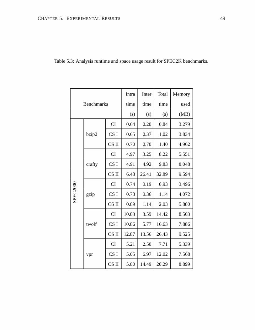
CHAPTER 5. EXPERIMENTAL RESULTS 49
Table 5.3: Analysis runtime and space usage result for SPEC2K benchmarks.
Intra Inter Total Memory
Benchmarks time time time used
(s) (s) (s) (MB)
SPE
C20
00
bzip2
CI 0.64 0.20 0.84 3.279
CS I 0.65 0.37 1.02 3.834
CS II 0.70 0.70 1.40 4.962
crafty
CI 4.97 3.25 8.22 5.551
CS I 4.91 4.92 9.83 8.048
CS II 6.48 26.41 32.89 9.594
gzip
CI 0.74 0.19 0.93 3.496
CS I 0.78 0.36 1.14 4.072
CS II 0.89 1.14 2.03 5.880
twolf
CI 10.83 3.59 14.42 8.503
CS I 10.86 5.77 16.63 7.886
CS II 12.87 13.56 26.43 9.525
vpr
CI 5.21 2.50 7.71 5.339
CS I 5.05 6.97 12.02 7.568
CS II 5.80 14.49 20.29 8.899
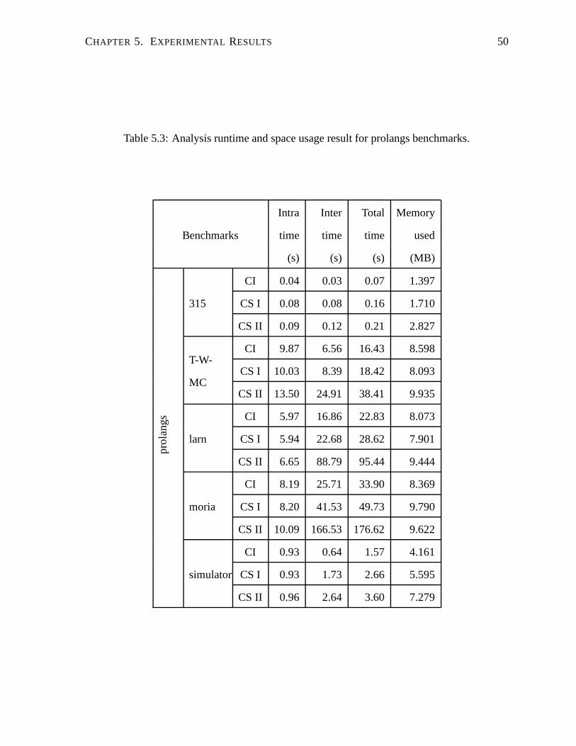
CHAPTER 5. EXPERIMENTAL RESULTS 50
Table 5.3: Analysis runtime and space usage result for prolangs benchmarks.
Intra Inter Total Memory
Benchmarks time time time used
(s) (s) (s) (MB)
prol
angs
315
CI 0.04 0.03 0.07 1.397
CS I 0.08 0.08 0.16 1.710
CS II 0.09 0.12 0.21 2.827
T-W-
MC
CI 9.87 6.56 16.43 8.598
CS I 10.03 8.39 18.42 8.093
CS II 13.50 24.91 38.41 9.935
larn
CI 5.97 16.86 22.83 8.073
CS I 5.94 22.68 28.62 7.901
CS II 6.65 88.79 95.44 9.444
moria
CI 8.19 25.71 33.90 8.369
CS I 8.20 41.53 49.73 9.790
CS II 10.09 166.53 176.62 9.622
simulator
CI 0.93 0.64 1.57 4.161
CS I 0.93 1.73 2.66 5.595
CS II 0.96 2.64 3.60 7.279

CHAPTER 5. EXPERIMENTAL RESULTS 51
0
20
40
60
80
100
120
140
160
180
Tim
e (
s )
Contexts101 102 103 104 105 106 107 108 109
Total Analysis TimeInvocation Graph Construction Time
PSfrag replacements
x20
x10
x21
x11
x22
x12
x23
x13
x24
x14
y1
y∗1
y2
y∗2
y3
y∗3
λ0
θ0
λ1
θ1
θ2
λ2
θ3
λ∗0
θ∗0
λ∗1
θ∗1
θ∗2
λ∗2
θ∗3
a
g
r
t
p
q
h1
h2
f
h
m
p1
q1
A
B
C
D
E
F
A0
B0
C0
D0
E0
F0
C1
D1
E1
F1
Figure 5.2: Algorithm runtime versus context count.
at most six times slower than its context-insensitive counterpart. Figure 5.2 offers more insight
on the dependency of total analysis time versus context count. Once again, the horizontal axis
shows the number of contexts in the evaluated benchmarks, which is the number of invocation
graph nodes, in log scale. The runtime for the pointer analysis, as well as the construction time
of the symbolic invocation graph, for a particular context number, are plotted.
Although the runtime increases with the context count, it can be seen in Figure 5.2 that the
symbolic invocation graph construction does not cause the jump in runtime. It is clear that even
for a benchmark with half a billion contexts, the symbolic invocation graph can be constructed
in a few seconds. We attribute the increase in runtime to the binding at each call site, and the
transfer function application.
5.3 Precision
Many studies have been performed on the impact of context-sensitivity on analysis precision
[36, 20]. Since this study focuses on the runtime of symbolic analysis, other analysis dimen-
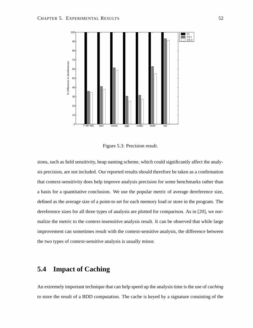
CHAPTER 5. EXPERIMENTAL RESULTS 52
0
10
20
30
40
50
60
70
80
90
100
% D
iffer
ence
in d
eref
eren
ces
T−W−MC larn moria pgp crafty twolf vpr
CICS ICS II
PSfrag replacements
x20
x10
x21
x11
x22
x12
x23
x13
x24
x14
y1
y∗1
y2
y∗2
y3
y∗3
λ0
θ0
λ1
θ1
θ2
λ2
θ3
λ∗0
θ∗0
λ∗1
θ∗1
θ∗2
λ∗2
θ∗3
a
g
r
t
p
q
h1
h2
f
h
m
p1
q1
A
B
C
D
E
F
A0
B0
C0
D0
E0
F0
C1
D1
E1
F1
Figure 5.3: Precision result.
sions, such as field sensitivity, heap naming scheme, which could significantly affect the analy-
sis precision, are not included. Our reported results should therefore be taken as a confirmation
that context-sensitivity does help improve analysis precision for some benchmarks rather than
a basis for a quantitative conclusion. We use the popular metric of average dereference size,
defined as the average size of a point-to set for each memory load or store in the program. The
dereference sizes for all three types of analysis are plotted for comparison. As in [20], we nor-
malize the metric to the context-insensitive analysis result. It can be observed that while large
improvement can sometimes result with the context-sensitive analysis, the difference between
the two types of context-sensitive analysis is usually minor.
5.4 Impact of Caching
An extremely important technique that can help speed up the analysis time is the use of caching
to store the result of a BDD computation. The cache is keyed by a signature consisting of the
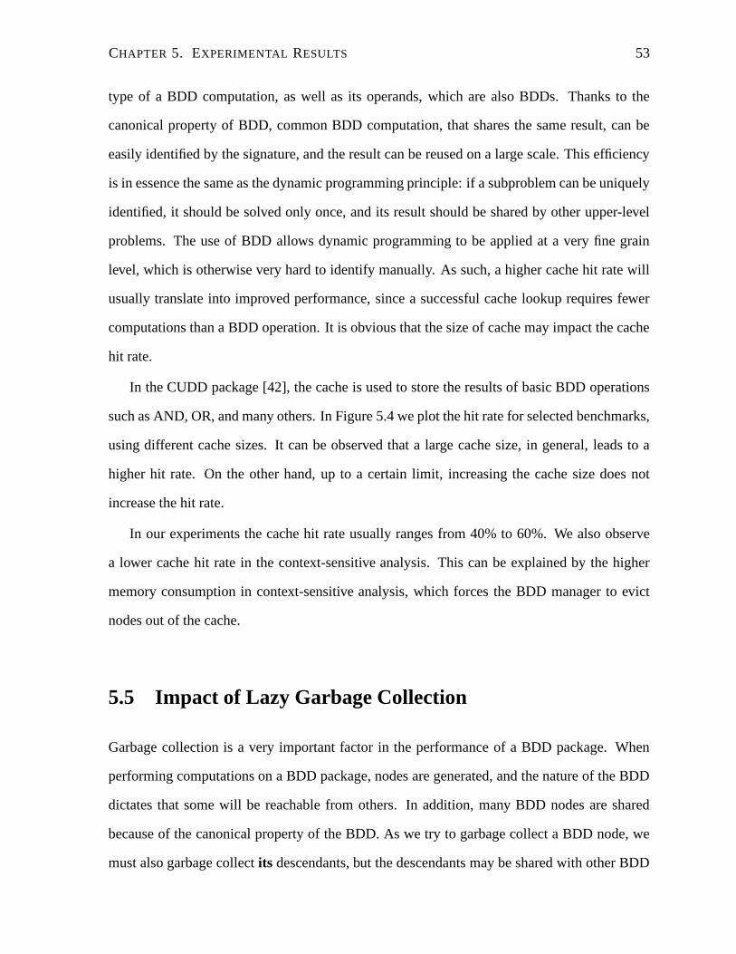
CHAPTER 5. EXPERIMENTAL RESULTS 53
type of a BDD computation, as well as its operands, which are also BDDs. Thanks to the
canonical property of BDD, common BDD computation, that shares the same result, can be
easily identified by the signature, and the result can be reused on a large scale. This efficiency
is in essence the same as the dynamic programming principle: if a subproblem can be uniquely
identified, it should be solved only once, and its result should be shared by other upper-level
problems. The use of BDD allows dynamic programming to be applied at a very fine grain
level, which is otherwise very hard to identify manually. As such, a higher cache hit rate will
usually translate into improved performance, since a successful cache lookup requires fewer
computations than a BDD operation. It is obvious that the size of cache may impact the cache
hit rate.
In the CUDD package [42], the cache is used to store the results of basic BDD operations
such as AND, OR, and many others. In Figure 5.4 we plot the hit rate for selected benchmarks,
using different cache sizes. It can be observed that a large cache size, in general, leads to a
higher hit rate. On the other hand, up to a certain limit, increasing the cache size does not
increase the hit rate.
In our experiments the cache hit rate usually ranges from 40% to 60%. We also observe
a lower cache hit rate in the context-sensitive analysis. This can be explained by the higher
memory consumption in context-sensitive analysis, which forces the BDD manager to evict
nodes out of the cache.
5.5 Impact of Lazy Garbage Collection
Garbage collection is a very important factor in the performance of a BDD package. When
performing computations on a BDD package, nodes are generated, and the nature of the BDD
dictates that some will be reachable from others. In addition, many BDD nodes are shared
because of the canonical property of the BDD. As we try to garbage collect a BDD node, we
must also garbage collect its descendants, but the descendants may be shared with other BDD

CHAPTER 5. EXPERIMENTAL RESULTS 54
0
10
20
30
40
50
60
70
80
Hit
%
T−W−MC larn moria pgp crafty twolf vpr
1 MB10 MB20 MB30 MB
PSfrag replacements
x20
x10
x21
x11
x22
x12
x23
x13
x24
x14
y1
y∗1
y2
y∗2
y3
y∗3
λ0
θ0
λ1
θ1
θ2
λ2
θ3
λ∗0
θ∗0
λ∗1
θ∗1
θ∗2
λ∗2
θ∗3
a
g
r
t
p
q
h1
h2
f
h
m
p1
q1
A
B
C
D
E
F
A0
B0
C0
D0
E0
F0
C1
D1
E1
F1
Figure 5.4: Cache hit rate.
nodes. Hence, while the canonical property contributes to the space efficiency of the BDD, it
makes garbage collection difficult.
The CUDD uses a technique called lazy garbage collection, keeping a reference count for
each BDD node. When the reference count of a BDD node goes to zero, its memory needs to
be reclaimed, or garbage collected. On the other hand, there is a high chance that this BDD
node may be re-created later. The CUDD package uses garbage collection lazily, that is, heap
space for nodes is reclaimed only when a threshold value of heap size is exceeded.
To see how lazy garbage collection can affect analysis speed, we demonstrate the time spent
on garbage collection, versus other processing time, for selected benchmarks, under different
threshold heap size values. The results are plotted in Figure 5.5, where the horizontal axis
lists the benchmarks, and the vertical axis shows the time spent in either garbage collection or
processing. It can be observed that in general a larger heap size will reduce the amount of time
spent on garbage collection, and therefore, the overall analysis speed. On the other hand, there
is almost nothing to gain if the threshold is increased beyond a certain value.
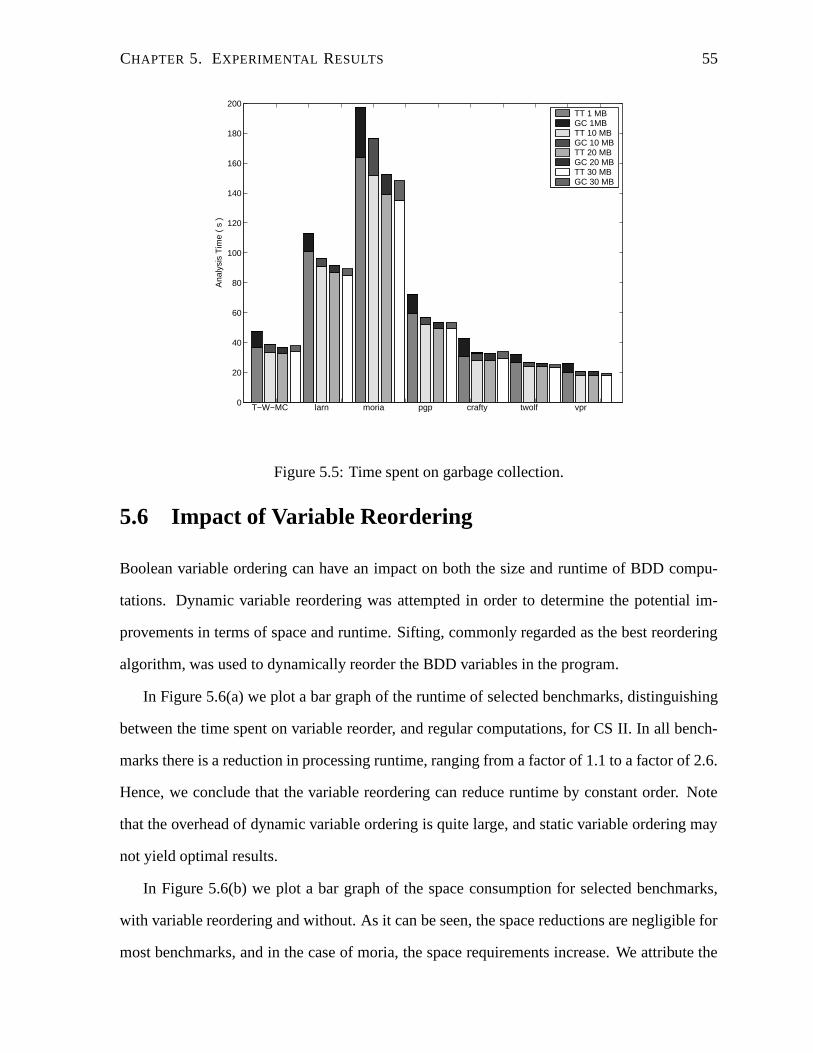
CHAPTER 5. EXPERIMENTAL RESULTS 55
0
20
40
60
80
100
120
140
160
180
200
Ana
lysi
s T
ime
( s
)
T−W−MC larn moria pgp crafty twolf vpr
TT 1 MBGC 1MBTT 10 MBGC 10 MBTT 20 MBGC 20 MBTT 30 MBGC 30 MB
PSfrag replacements
x20
x10
x21
x11
x22
x12
x23
x13
x24
x14
y1
y∗1
y2
y∗2
y3
y∗3
λ0
θ0
λ1
θ1
θ2
λ2
θ3
λ∗0
θ∗0
λ∗1
θ∗1
θ∗2
λ∗2
θ∗3
a
g
r
t
p
q
h1
h2
f
h
m
p1
q1
A
B
C
D
E
F
A0
B0
C0
D0
E0
F0
C1
D1
E1
F1
Figure 5.5: Time spent on garbage collection.
5.6 Impact of Variable Reordering
Boolean variable ordering can have an impact on both the size and runtime of BDD compu-
tations. Dynamic variable reordering was attempted in order to determine the potential im-
provements in terms of space and runtime. Sifting, commonly regarded as the best reordering
algorithm, was used to dynamically reorder the BDD variables in the program.
In Figure 5.6(a) we plot a bar graph of the runtime of selected benchmarks, distinguishing
between the time spent on variable reorder, and regular computations, for CS II. In all bench-
marks there is a reduction in processing runtime, ranging from a factor of 1.1 to a factor of 2.6.
Hence, we conclude that the variable reordering can reduce runtime by constant order. Note
that the overhead of dynamic variable ordering is quite large, and static variable ordering may
not yield optimal results.
In Figure 5.6(b) we plot a bar graph of the space consumption for selected benchmarks,
with variable reordering and without. As it can be seen, the space reductions are negligible for
most benchmarks, and in the case of moria, the space requirements increase. We attribute the

CHAPTER 5. EXPERIMENTAL RESULTS 56
0
20
40
60
80
100
120
140
160
180
200
Tim
e (
s )
T−W−MC larn moria pgp crafty twolf vpr
OtherReordering
PSfrag replacements
x20
x10
x21
x11
x22
x12
x23
x13
x24
x14
y1
y∗1
y2
y∗2
y3
y∗3
λ0
θ0
λ1
θ1
θ2
λ2
θ3
λ∗0
θ∗0
λ∗1
θ∗1
θ∗2
λ∗2
θ∗3
a
g
r
t
p
q
h1
h2
f
h
m
p1
q1
A
B
C
D
E
F
A0
B0
C0
D0
E0
F0
C1
D1
E1
F1
(a) Time spent on variable reordering.
0
2
4
6
8
10
12
Mem
ory
(MB
)
T-W-MC larn moria pgp crafty twolf vpr
Reordered Not Reordered
PSfrag replacements
x20
x10
x21
x11
x22
x12
x23
x13
x24
x14
y1
y∗1
y2
y∗2
y3
y∗3
λ0
θ0
λ1
θ1
θ2
λ2
θ3
λ∗0
θ∗0
λ∗1
θ∗1
θ∗2
λ∗2
θ∗3
a
g
r
t
p
q
h1
h2
f
h
m
p1
q1
A
B
C
D
E
F
A0
B0
C0
D0
E0
F0
C1
D1
E1
F1
(b) Memory size with/without variable reorder-
ing.
Figure 5.6: Variable Reordering
space increase in moria to a tradeoff involving the runtime decrease shown in Figure 5.6(a).
Chapter 6
Conclusion
In this thesis, we present a new Boolean formalism for pointer analysis. The Boolean formal-
ism enables the use of Binary Decision Diagram to achieve both space and speed efficiency.
In addition, we introduce the concept of the symbolic invocation graph, which reduces the ex-
ponential complexity of the invocation graph construction into a polynomial complexity with
respect to the number of call graph nodes. We further introduce the concept of state super-
position, allowing us to represent the state of an arbitrary number of procedure invocations in
one Boolean formula. Using these concepts, we derive a common framework for both context-
sensitive and context-insensitive pointer analysis.
Based on our study, we conclude that the key concepts proposed, namely symbolic transfer
function and symbolic invocation graph, can effectively reduce the runtime of the otherwise
expensive context-sensitive analysis to one comparable to its context-insensitive counterpart.
From this work we gained much insight into the use of the symbolic method for pointer
analysis. In the future we plan on leveraging this knowledge, and in particular, modifying
the Boolean formalism to perform the entire pointer analysis symbolically. There are many
other precision improvements to consider as well. For instance, using the symbolic method
to compute a flow-sensitive pointer analysis solution. In addition, we can consider field-
sensitivity, which distinguishes between record fields of a data structure, and more importantly,
57

CHAPTER 6. CONCLUSION 58
the iteration-sensitive pointer analysis, which distinguishes between various array elements.
Bibliography
[1] SPEC CPU2000 benchmarks. http://www.specbench.org/cpu2000/.
[2] S. B. Akers. Binary decision diagrams. IEEE Transactions on Computer, C-27(6):509–
516, June 1978.
[3] Aleph One. Smashing the stack for fun and profit. Phrack, 7(49), November 1996.
[4] O. Andersen. Program Analysis and Specialization for the C Programming Language.
PhD thesis, Computer Science Department, University of Copenhagen, 1994.
[5] Thomas Ball and Todd Millstein. Polymorphic predicate abstraction. Technical Report
MSR-TR-2001-10, Microsoft Research, June 24, 2003.
[6] C. Leonard Berman. Circuit width, register allocation, and ordered binary decision dia-
grams. IEEE Transactions on Computer-Aided Design of Integrated Circuits and Systems,
pages 1059–1066, August 1991.
[7] Marc Berndl, Ondrej Lhotak, Feng Qian, Laurie Hendren, and Navindra Umanee. Point-
to analysis using BDD. In Proceedings of the ACM SIGPLAN Conference on Program-
ming Language Design and Implementation, San Diego, June 2003.
[8] Randal E. Bryant. Graph-based algorithms for Boolean function manipulation. IEEE
Transactions on Computer, C-35(8):677–691, August 1986.
59
BIBLIOGRAPHY 60
[9] J. R. Burch, E. M. Clarke, and D. E. Long. Symbolic model checking with partitioned
transition relations. In International Conference on Very Large Scale Integration, Edin-
burgh, Scotland, 1991.
[10] J. R. Burch, E. M. Clarke, D. E. Long, K. L. McMillan, and D. L. Dill. Symbolic model
checking for sequential circuit verification. IEEE Transactions on Computer-Aided De-
sign of Integrated Circuits and Systems, (13), 1994.
[11] J. R. Burch, E. M. Clarke, K. L. McMillan, D. L. Dill, and L. J. Hwang. Symbolic model
checking: 1020 states and beyond. In Proceedings of the Fifth Annual IEEE Symposium
on Logic in Computer Science, Washington, DC, 1990.
[12] R. Chatterjee, B. G. Ryder, and W. A. Landi. Relevant context inference. In Proceedings
of Symposium on Principles of Programming Languages, pages 133–146, 1999.
[13] Ben-Chung Cheng and Wen-Mei W. Hwu. Modular interprocedural pointer analysis us-
ing access paths: Design implementation and evaluation. In Proceedings of SIGPLAN
Conference on Programming Language Design and Implementation, pages 57–69, Van-
couver, British Columbia, Canada, June 2000.
[14] O. Coudert, C. Berthet, and J. C. Madre. A unified framework for the formal verification
of sequential circuits. In Proceedings of the International Conference on Computer-Aided
Design, pages 126–129, November 1990.
[15] O. Coudert and J. C. Madre. Symbolic computation of the valid states of a sequential
machine: Algorithms and discussion. In ACM Workshop on Formal Methods in VLSI
Design, 1991.
[16] Manuvir Das. Unification-based pointer analysis with directional assignments. ACM
SIGPLAN Notices, 35(5):35–46, 2000.
BIBLIOGRAPHY 61
[17] Maryam Emami, Rakesh Ghiya, and Laurie J. Hendren. Context-sensitive interprocedural
points-to analysis in the presence of function pointers. In Proceedings of SIGPLAN Con-
ference on Programming Language Design and Implementation, pages 242–256, 1994.
[18] M. Fahndrich, J. Rehof, and M. Das. Scalable context-sensitive flow analysis using instan-
tiation constraints. In Proceedings of the ACM SIGPLAN Conference on Programming
Language Design and Implementation, pages 253–263, Vancouver, British Columbia,
Canada, June 2000.
[19] Manuel Fahndrich, Jeffrey S. Foster, Zhendong Su, and Alexander Aiken. Partial online
cycle elimination in inclusion constraint graphs. ACM SIGPLAN Notices, 33(5):85–96,
1998.
[20] J. S. Foster, M. Fahndrich, and A. Aiken. Polymorphic versus monomorphic flow-
insensitive points-to analysis for C. In Proceedings of Static Analysis Symposium, pages
175–198, June 2000.
[21] D. Gajski. Principles of Digital Design. Prentice Hall, 1997.
[22] Nevin Heintze and Olivier Tardieu. Demand-driven pointer analysis. In Proceedings
of SIGPLAN Conference on Programming Language Design and Implementation, pages
24–34, 2001.
[23] Michael Hind. Pointer analysis: Haven’t we solved this problem yet. In ACM SIGPLAN-
SIGSOFT Workshop on Program Analysis for Software Tools and Engineering (PASTE),
June 2001.
[24] Michael Hind, Michael Burke, Paul Carini, and Jong-Deok Choi. Interprocedural pointer
alias analysis. ACM Transactions on Programming Languages and Systems, 21(4):848–
894, 1999.
BIBLIOGRAPHY 62
[25] Michael Hind and Anthony Pioli. Assessing the effects of flow-sensitivity on pointer alias
analyses. In Proceedings of Static Analysis Symposium, pages 57–81, 1998.
[26] Michael Hind and Anthony Pioli. Which pointer analysis should I use? In International
Symposium on Software Testing and Analysis, pages 113–123, 2000.
[27] Martin Hirzel. Connectivity-Based Garbage Collection. PhD thesis, Computer Science
Department, University of Colorado, 2004.
[28] Robert van Engelen Johnnie Birch and Kyle Gallivan. Value range analysis of condition-
ally updated variables and pointers. In Compilers for Parallel Computing (CPC), pages
265–276, 2004.
[29] C. Lee, M. Potkonjak, and W. H. Mangione-Smith. Mediabench: A tool for evaluating
and synthesizing multimedia and communications systems. In Micro 30, 1997.
[30] X. Leroy. An overview of types in compilation, 1998.
[31] Ondrej Lhotak and Laurie Hendren. Jedd: A BDD-based relational extension of Java. In
Proceedings of SIGPLAN Conference on Programming Language Design and Implemen-
tation, June 2004.
[32] Donglin Liang and Mary Jean Harrold. Efficient computation of parameterized pointer
information for interprocedural analyses. In Proceedings of Static Analysis Symposium,
pages 279–298, 2001.
[33] In-Ho Moon, James H. Kukula, Kavita Ravi, and Fabio Somenzi. To split or to conjoin:
the question in image computation. In Design Automation Conference, pages 23–28,
2000.
[34] P. Panda, L. Semeria, and G. De Micheli. Cache-efficient memory layout of aggregate
data structures. In Proceedings of the International Symposium on System Synthesis,
September 2001.
BIBLIOGRAPHY 63
[35] Atanas Rountev and Satish Chandra. Off-line variable substitution for scaling points-to
analysis. ACM SIGPLAN Notices, 35(5):47–56, 2000.
[36] Erik Ruf. Context-insensitive alias analysis reconsidered. In Proceedings of SIGPLAN
Conference on Programming Language Design and Implementation, pages 13–22, La
Jolla, California, June 1995.
[37] Barbara Ryder. Prolangs analysis framework. http://www.prolangs.rutgers.
edu.
[38] Mooly Sagiv, Thomas Reps, and Reinhard Wilhelm. Parametric shape analysis via 3-
valued logic. ACM Transactions on Programming Languages and Systems, 24(3):217–
298, 2002.
[39] L. Semeria and G. De Micheli. Resolution, optimization, and encoding of pointer vari-
ables for the behavioral synthesis from c. IEEE Transactions on Computer-Aided Design
of Integrated Circuits and Systems, February 2001.
[40] L. Semeria, K. Sata, and G. De Micheli. Synthesis of hardware models in C with pointers
and complex data structures. IEEE Transactions on Computer-Aided Design of Integrated
Circuits and Systems, February 2001.
[41] Luc Semeria. Applying Pointer Analysis To The Synthesis of Hardware From C. PhD
thesis, Department of Electrical Engineering, Stanford University, 2001.
[42] F. Somenzi. CUDD: Binary decision diagram package release. http://vlsi.
Colorado.EDU/˜fabio/CUDD/cuddIntro.html, 1998.
[43] Bjarne Steensgaard. Points-to analysis in almost linear time. In Proceedings of Sympo-
sium on Principles of Programming Languages, pages 32–41, 1996.
[44] R. Tarjan. Depth first search and linear graph algorithms. SIAM Journal of Computing,
1(2):146–160, 1972.
BIBLIOGRAPHY 64
[45] Robert Endre Tarjan. Efficiency of a good but not linear set union algorithm. J. ACM,
22(2):215–225, 1975.
[46] Philip L. Wadler. Fixing some space leaks with a garbage collector. Software Practice
and Experience, 17(9):595–609, 1987.
[47] John Whaley and Monica Lam. Cloning-based context-sensitive pointer alias analysis us-
ing binary decision diagrams. In Proceedings of SIGPLAN Conference on Programming
Language Design and Implementation, June 2004.
[48] R. Wilson and M. Lam. Efficient context-sensitive pointer analysis for C programs. In
Proceedings of the ACM SIGPLAN Conference on Programming Language Design and
Implementation, pages 1–12, June 1995.
[49] J. Zhu. Symbolic pointer analysis. In Proceedings of the International Conference in
Computer Aided Design, San Jose, November 2002.
[50] Jianwen Zhu and Silvian Calman. Symbolic pointer analysis revisited. In Proceedings
of SIGPLAN Conference on Programming Language Design and Implementation, June
2004.
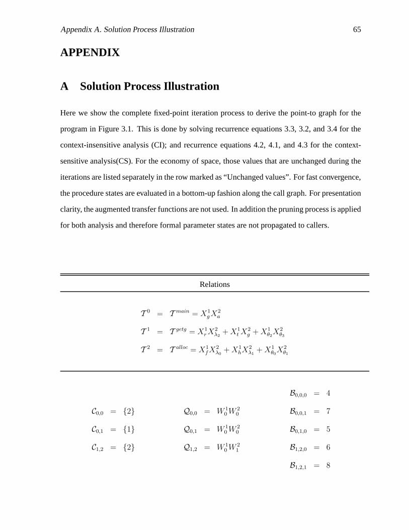
Appendix A. Solution Process Illustration 65
APPENDIX
A Solution Process Illustration
Here we show the complete fixed-point iteration process to derive the point-to graph for the
program in Figure 3.1. This is done by solving recurrence equations 3.3, 3.2, and 3.4 for the
context-insensitive analysis (CI); and recurrence equations 4.2, 4.1, and 4.3 for the context-
sensitive analysis(CS). For the economy of space, those values that are unchanged during the
iterations are listed separately in the row marked as “Unchanged values”. For fast convergence,
the procedure states are evaluated in a bottom-up fashion along the call graph. For presentation
clarity, the augmented transfer functions are not used. In addition the pruning process is applied
for both analysis and therefore formal parameter states are not propagated to callers.
Relations
T 0 = T main = X1gX2
a
T 1 = T getg = X1r X2
λ2+ X1
t X2g + X1
θ2X2
θ3
T 2 = T alloc = X1fX2
λ0+ X1
hX2λ1
+ X1θ0
X2θ1
C0,0 = {2}
C0,1 = {1}
C1,2 = {2}
Q0,0 = W 10 W 2
0
Q0,1 = W 10 W 2
0
Q1,2 = W 10 W 2
1
B0,0,0 = 4
B0,0,1 = 7
B0,1,0 = 5
B1,2,0 = 6
B1,2,1 = 8
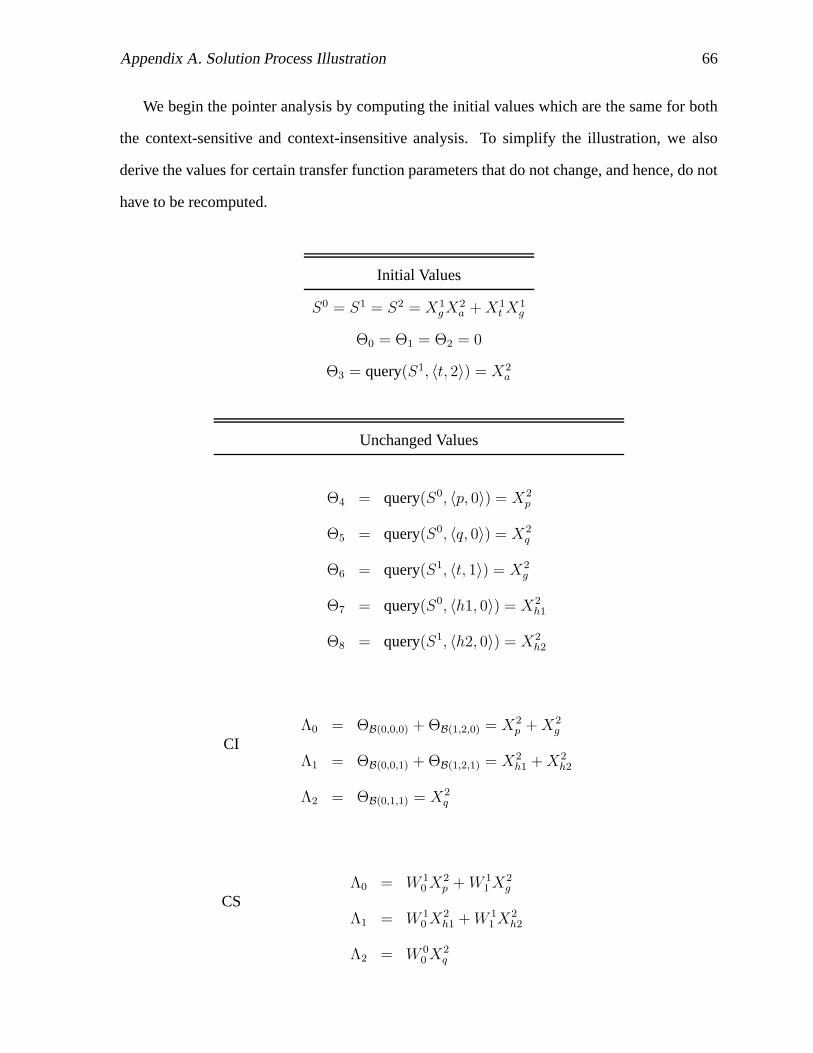
Appendix A. Solution Process Illustration 66
We begin the pointer analysis by computing the initial values which are the same for both
the context-sensitive and context-insensitive analysis. To simplify the illustration, we also
derive the values for certain transfer function parameters that do not change, and hence, do not
have to be recomputed.
Initial Values
S0 = S1 = S2 = X1gX2
a + X1t X1
g
Θ0 = Θ1 = Θ2 = 0
Θ3 = query(S1, 〈t, 2〉) = X2a
Unchanged Values
Θ4 = query(S0, 〈p, 0〉) = X2p
Θ5 = query(S0, 〈q, 0〉) = X2q
Θ6 = query(S1, 〈t, 1〉) = X2g
Θ7 = query(S0, 〈h1, 0〉) = X2h1
Θ8 = query(S1, 〈h2, 0〉) = X2h2
CIΛ0 = ΘB(0,0,0) + ΘB(1,2,0) = X2
p + X2g
Λ1 = ΘB(0,0,1) + ΘB(1,2,1) = X2h1 + X2
h2
Λ2 = ΘB(0,1,1) = X2q
CSΛ0 = W 1
0 X2p + W 1
1 X2g
Λ1 = W 10 X2
h1 + W 11 X2
h2
Λ2 = W 00 X2
q
Appendix A. Solution Process Illustration 67
The recurrence equations for both the context-insensitive and context-sensitive pointer anal-
ysis are solved in the next two pages. Note that the fixed-point is reached after 4 iterations. In
the context-sensitive analysis p does not point-to h2. Furthermore, g does not point-to h1, and
as such, q does not point-to h1 as well. Thus, the context-sensitive pointer analysis improves
precision over the context-insensitive counterpart for the program in Figure 3.1.
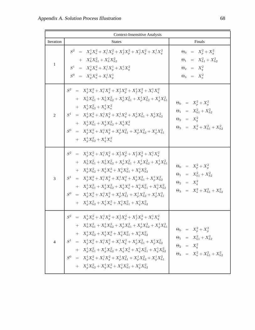
Appendix A. Solution Process Illustration 68
Context-Insensitive Analysis
Iteration States Finals
1
S2 = X1gX2
a + X1t X2
g + X1fX2
p + X1f X2
g + X1r X2
q
+ X1hX2
h1 + X1hX2
h2
S1 = X1gX2
a + X1t X1
g + X1r X2
q
S0 = X1gX2
a + X1t X1
g
Θ0 = X2p + X2
g
Θ1 = X2h1 + X2
h2
Θ2 = X2q
Θ3 = X2a
2
S2 = X1g X2
a + X1t X2
g + X1f X2
p + X1fX2
g + X1r X2
q
+ X1hX2
h1 + X1hX2
h2 + X1pX2
h1 + X1pX2
h2 + X1gX2
h1
+ X1g X2
h2 + X1q X2
a
S1 = X1g X2
a + X1t X2
g + X1r X2
q + X1pX2
h1 + X1pX2
h2
+ X1g X2
h1 + X1g X2
h2 + X1q X2
a
S0 = X1g X2
a + X1t X2
g + X1pX2
h1 + X1pX2
h2 + X1g X2
h1
+ X1g X2
h2 + X1q X2
a
Θ0 = X2p + X2
g
Θ1 = X2h1 + X2
h2
Θ2 = X2q
Θ3 = X2a + X2
h1 + X2h2
3
S2 = X1g X2
a + X1t X2
g + X1f X2
p + X1fX2
g + X1r X2
q
+ X1hX2
h1 + X1hX2
h2 + X1pX2
h1 + X1pX2
h2 + X1gX2
h1
+ X1g X2
h2 + X1q X2
a + X1q X2
h1 + X1q X2
h2
S1 = X1g X2
a + X1t X2
g + X1r X2
q + X1pX2
h1 + X1pX2
h2
+ X1g X2
h1 + X1g X2
h2 + X1q X2
a + X1q X2
h1 + X1q X2
h2
S0 = X1g X2
a + X1t X2
g + X1pX2
h1 + X1pX2
h2 + X1g X2
h1
+ X1g X2
h2 + X1q X2
a + X1q X2
h1 + X1q X2
h2
Θ0 = X2p + X2
g
Θ1 = X2h1 + X2
h2
Θ2 = X2q
Θ3 = X2a + X2
h1 + X2h2
4
S2 = X1g X2
a + X1t X2
g + X1f X2
p + X1fX2
g + X1r X2
q
+ X1hX2
h1 + X1hX2
h2 + X1pX2
h1 + X1pX2
h2 + X1gX2
h1
+ X1g X2
h2 + X1q X2
a + X1q X2
h1 + X1q X2
h2
S1 = X1g X2
a + X1t X2
g + X1r X2
q + X1pX2
h1 + X1pX2
h2
+ X1g X2
h1 + X1g X2
h2 + X1q X2
a + X1q X2
h1 + X1q X2
h2
S0 = X1g X2
a + X1t X2
g + X1pX2
h1 + X1pX2
h2 + X1g X2
h1
+ X1g X2
h2 + X1q X2
a + X1q X2
h1 + X1q X2
h2
Θ0 = X2p + X2
g
Θ1 = X2h1 + X2
h2
Θ2 = X2q
Θ3 = X2a + X2
h1 + X2h2

Appendix A. Solution Process Illustration 69
Context-Sensitive Analysis
Iteration States Finals
1
S2 = X1gX2
a + X1t X2
g + W 10 X1
fX2p + W 1
1 X1fX2
g
+ W 10 X1
r X2q + W 1
0 X1hX2
h1 + W 11 X1
hX2h2
S1 = X1gX2
a + X1t X1
g + W 10 X1
r X2q
S0 = X1gX2
a + X1t X1
g
Θ0 = W 10 X2
p + W 11 X2
g
Θ1 = W 10 X2
h1 + W 11 X2
h2
Θ2 = W 10 X2
q
Θ3 = X2a
2
S2 = X1g X2
a + X1t X2
g + W 10 X1
fX2p + W 1
1 X1f X2
g
+ W 11 X1
r X2q + W 1
0 X1hX2
h1 + W 11 X1
hX2h2
+ (W 11 + W 1
0 ) · (X1q X2
a + X1pX2
h1 + X1g X2
h2)
S1 = X1g X2
a + X1t X2
g + W 10 X1
r X2q + W 1
0 X1pX2
h1
+ W 10 X1
g X2h2 + W 1
0 X1q X2
a
S0 = X1g X2
a + X1t X2
g + W 10 X1
pX2h1 + W 1
0 X1gX2
h2
+ W 10 X1
q X2a
Θ0 = W 10 X2
p + W 11 X2
g
Θ1 = W 10 X2
h1 + W 11 X2
h2
Θ2 = W 10 X2
q
Θ3 = X2a + W 1
0 X2h1
+ W 11 X2
h2
3
S2 = X1g X2
a + X1t X2
g + W 10 X1
fX2p + W 1
1 X1f X2
g
+ W 10 X1
r X2q + W 1
0 X1hX2
h1 + W 11 X1
hX2h2
+ (W 11 + W 1
0 ) · (X1q X2
a + X1pX2
h1 + X1g X2
h2 + X1q X2
h2)
S1 = X1g X2
a + X1t X2
g + W 10 X1
r X2q + W 1
0 X1pX2
h1
+ W 10 X1
g X2h2 + W 1
0 X1q X2
a + W 10 X1
q X2h2
S0 = X1g X2
a + X1t X2
g + W 10 X1
pX2h1 + W 1
0 X1gX2
h2
+ W 10 X1
q X2a + W 1
0 X1q X2
h2
Θ0 = W 10 X2
p + W 11 X2
g
Θ1 = W 10 X2
h1 + W 11 X2
h2
Θ2 = W 10 X2
q
Θ3 = X2a + W 1
0 X2h1
+ W 11 X2
h2
4
S2 = X1g X2
a + X1t X2
g + W 10 X1
fX2p + W 1
1 X1f X2
g
+ W 10 X1
r X2q + W 1
0 X1hX2
h1 + W 11 X1
hX2h2
+ (W 11 + W 1
0 ) · (X1q X2
a + X1pX2
h1 + X1g X2
h2 + X1q X2
h2)
S1 = X1g X2
a + X1t X2
g + W 10 X1
r X2q + W 1
0 X1pX2
h1
+ W 10 X1
g X2h2 + W 1
0 X1q X2
a + W 10 X1
q X2h2
S0 = X1g X2
a + X1t X2
g + W 10 X1
pX2h1 + W 1
0 X1gX2
h2
+ W 10 X1
q X2a + W 1
0 X1q X2
h2
Θ0 = W 10 X2
p + W 11 X2
g
Θ1 = W 10 X2
h1 + W 11 X2
h2
Θ2 = W 10 X2
q
Θ3 = X2a + W 1
0 X2h1
+ W 11 X2
h2