symmetries, fields and particles - damtp · 7.2 a non-abelian gauge theory: ... the lepton number...

University of Cambridge

Part III of the Mathematical Tripos

Symmetries, Fields and ParticlesMichaelmas 2014, Prof. N. Manton

Notes by:William I. Jay

Diagrams by:Ben Nachman

Edited and updated by:Nicholas S. Manton

Last updated on September 23, 2014

Preface

William Jay typeset these notes from the Cambridge Mathematics Part III course Symmetries,Fields and Particles in Spring 2013. Some material amplifies or rephrases the lectures.N. Manton edited and updated these notes in Autumn 2013, with further minor changes in Autumn2014. If you find errors, please contact [email protected].

Thanks to Ben Nachman for producing all of the diagrams in these notes.

1

Contents

1 Introduction to Particles 51.1 Standard Model Fields . . . . . . . . . . . . . . . . . . . . . . . . . . . . . . . . . . . 5

1.1.1 Fermions: Spin 1/2 (“matter”) . . . . . . . . . . . . . . . . . . . . . . . . . . 51.1.2 Bosons: Spin 0 or 1 . . . . . . . . . . . . . . . . . . . . . . . . . . . . . . . . 6

1.2 Observed Particles (of “long life”) . . . . . . . . . . . . . . . . . . . . . . . . . . . . 61.3 Further Remarks on Particles . . . . . . . . . . . . . . . . . . . . . . . . . . . . . . . 6

1.3.1 Mass of gauge bosons . . . . . . . . . . . . . . . . . . . . . . . . . . . . . . . 61.3.2 The Poincare Symmetry . . . . . . . . . . . . . . . . . . . . . . . . . . . . . . 61.3.3 Approximate Symmetries . . . . . . . . . . . . . . . . . . . . . . . . . . . . . 7

1.4 Particle Models . . . . . . . . . . . . . . . . . . . . . . . . . . . . . . . . . . . . . . . 71.5 Forces and Processes . . . . . . . . . . . . . . . . . . . . . . . . . . . . . . . . . . . . 7

1.5.1 Strong Nuclear Force (quarks, gluons, SU(3) gauge fields) . . . . . . . . . . . 71.5.2 Electroweak Forces . . . . . . . . . . . . . . . . . . . . . . . . . . . . . . . . . 8

2 Symmetry 102.1 Symmetry . . . . . . . . . . . . . . . . . . . . . . . . . . . . . . . . . . . . . . . . . . 10

3 Lie Groups and Lie Algebras 123.1 Subgroups of G . . . . . . . . . . . . . . . . . . . . . . . . . . . . . . . . . . . . . . . 123.2 Matrix Lie Groups . . . . . . . . . . . . . . . . . . . . . . . . . . . . . . . . . . . . . 12

3.2.1 Important Subgroups of GL(n) . . . . . . . . . . . . . . . . . . . . . . . . . . 133.2.2 A Remark on Subgroups Defined Algebraically . . . . . . . . . . . . . . . . . 14

3.3 Lie Algebras . . . . . . . . . . . . . . . . . . . . . . . . . . . . . . . . . . . . . . . . . 153.3.1 Lie Algebra of SO(2) . . . . . . . . . . . . . . . . . . . . . . . . . . . . . . . . 153.3.2 Lie Algebra of SO(n) . . . . . . . . . . . . . . . . . . . . . . . . . . . . . . . 153.3.3 Lie algebra of SU(n) and U(n) . . . . . . . . . . . . . . . . . . . . . . . . . . 163.3.4 General Structure of L(G) for a matrix group G . . . . . . . . . . . . . . . . 173.3.5 SU(2) and SO(3): The Basic Non-abelian Lie Groups . . . . . . . . . . . . . 183.3.6 The Isomorphism SO(3) ' SU(2)/Z2 . . . . . . . . . . . . . . . . . . . . . . 19

3.4 Lie Group – Lie Algebra Relation . . . . . . . . . . . . . . . . . . . . . . . . . . . . . 193.4.1 Tangent space to G at general element g . . . . . . . . . . . . . . . . . . . . . 193.4.2 The Baker-Campbell-Hausdorff Formula . . . . . . . . . . . . . . . . . . . . . 21

4 Lie Group Actions: Orbits 224.1 Examples of Group Actions . . . . . . . . . . . . . . . . . . . . . . . . . . . . . . . . 224.2 The General Nature of an Orbit of G . . . . . . . . . . . . . . . . . . . . . . . . . . . 23

5 Representations of Lie Groups 255.1 Types of Representation . . . . . . . . . . . . . . . . . . . . . . . . . . . . . . . . . . 25

2

Part III Symmetries, Fields and Particles Section 0.0

6 Representations of Lie Algebras 286.1 Representation of L(G) from a Representation of G . . . . . . . . . . . . . . . . . . . 28

6.1.1 The adjoint representation of L(G) . . . . . . . . . . . . . . . . . . . . . . . . 296.2 Representation of G from a Representation of L(G) . . . . . . . . . . . . . . . . . . . 296.3 su(2): The Mathematics of Quantum Angular Momentum . . . . . . . . . . . . . . . 29

6.3.1 Irreducible Representations of su(2) . . . . . . . . . . . . . . . . . . . . . . . 306.4 Tensor Products of Representations . . . . . . . . . . . . . . . . . . . . . . . . . . . . 31

6.4.1 The Representation of L(G) associated to D(1) ⊗D(2) . . . . . . . . . . . . . 316.4.2 Tensor Products of su(2) Irreducible Representations . . . . . . . . . . . . . . 32

6.5 Roots and Weights for general L(G) . . . . . . . . . . . . . . . . . . . . . . . . . . . 32

7 Gauge Theories 347.1 Scalar Electrodynamics . . . . . . . . . . . . . . . . . . . . . . . . . . . . . . . . . . 34

7.1.1 Field Tensor from Covariant Derivatives . . . . . . . . . . . . . . . . . . . . . 367.2 A Non-Abelian Gauge Theory: Scalar Yang-Mills Theory . . . . . . . . . . . . . . . 36

7.2.1 Lagrangian Density . . . . . . . . . . . . . . . . . . . . . . . . . . . . . . . . 377.2.2 Adjoint Covariant Derivative . . . . . . . . . . . . . . . . . . . . . . . . . . . 387.2.3 General Covariant Derivative . . . . . . . . . . . . . . . . . . . . . . . . . . . 387.2.4 The Field Equation of Pure Yang-Mills Theory . . . . . . . . . . . . . . . . . 387.2.5 Classical Vacuum . . . . . . . . . . . . . . . . . . . . . . . . . . . . . . . . . . 38

7.3 A Very Brief Introduction to Mass and the Higgs Mechanism . . . . . . . . . . . . . 397.3.1 Electrodynamics . . . . . . . . . . . . . . . . . . . . . . . . . . . . . . . . . . 397.3.2 Perturbative Effect of Interaction of EM Field with a Charged Scalar Field . 407.3.3 Higgs Mechanism . . . . . . . . . . . . . . . . . . . . . . . . . . . . . . . . . . 407.3.4 Higgs Mechanism in the Non-abelian Case . . . . . . . . . . . . . . . . . . . . 41

8 Quadratic Forms on Lie Algebras and the Geometry of Lie Groups 428.1 Invariant Quadratic Forms . . . . . . . . . . . . . . . . . . . . . . . . . . . . . . . . . 428.2 Non-Degeneracy of the Killing Form . . . . . . . . . . . . . . . . . . . . . . . . . . . 438.3 Compactness . . . . . . . . . . . . . . . . . . . . . . . . . . . . . . . . . . . . . . . . 448.4 Universal Enveloping Algebra . . . . . . . . . . . . . . . . . . . . . . . . . . . . . . . 448.5 Casimir Elements . . . . . . . . . . . . . . . . . . . . . . . . . . . . . . . . . . . . . . 458.6 Metric on G . . . . . . . . . . . . . . . . . . . . . . . . . . . . . . . . . . . . . . . . . 468.7 Kinetic Energy and Geodesic Motion . . . . . . . . . . . . . . . . . . . . . . . . . . . 478.8 SU(2) Metric and Volume Form . . . . . . . . . . . . . . . . . . . . . . . . . . . . . 48

8.8.1 Euler Angle Parametrization . . . . . . . . . . . . . . . . . . . . . . . . . . . 48

9 SU(3) and its Representations 499.1 Roots . . . . . . . . . . . . . . . . . . . . . . . . . . . . . . . . . . . . . . . . . . . . 499.2 Representations and Weights . . . . . . . . . . . . . . . . . . . . . . . . . . . . . . . 51

9.2.1 General Constraint on Weights . . . . . . . . . . . . . . . . . . . . . . . . . . 529.2.2 Weights of some Irreps of su(3) . . . . . . . . . . . . . . . . . . . . . . . . . . 539.2.3 Conjugate Representations . . . . . . . . . . . . . . . . . . . . . . . . . . . . 539.2.4 Tensor Products for su(3) . . . . . . . . . . . . . . . . . . . . . . . . . . . . . 55

9.3 Quarks . . . . . . . . . . . . . . . . . . . . . . . . . . . . . . . . . . . . . . . . . . . . 569.3.1 Meson Octet . . . . . . . . . . . . . . . . . . . . . . . . . . . . . . . . . . . . 579.3.2 Baryon Octet and Decuplet . . . . . . . . . . . . . . . . . . . . . . . . . . . . 579.3.3 The Pauli Principle and Color . . . . . . . . . . . . . . . . . . . . . . . . . . 58

3 Typeset by W.I. Jay


10 Complexification of L(G), Representations 5910.1 L(G)C . . . . . . . . . . . . . . . . . . . . . . . . . . . . . . . . . . . . . . . . . . . 5910.2 L(G)C as a real Lie algebra <L(G)C . . . . . . . . . . . . . . . . . . . . . . . . . . 5910.3 Another Point of View . . . . . . . . . . . . . . . . . . . . . . . . . . . . . . . . . . . 60

11 Lorentz Group and Lie Algebra, Representations 62

12 Poincare Group and Particle States 6412.1 Lie algebra and Casimirs . . . . . . . . . . . . . . . . . . . . . . . . . . . . . . . . . . 6412.2 Representations . . . . . . . . . . . . . . . . . . . . . . . . . . . . . . . . . . . . . . . 65

12.2.1 General Idea of Induced Representation . . . . . . . . . . . . . . . . . . . . . 6512.2.2 Application to Representations of the Poincare Group . . . . . . . . . . . . . 6612.2.3 Irreducible Representations with Spin . . . . . . . . . . . . . . . . . . . . . . 6712.2.4 Massless Case . . . . . . . . . . . . . . . . . . . . . . . . . . . . . . . . . . . . 67


Chapter 1

Introduction to Particles

The Standard Model incorporates all the fundamental particles including the recently discoveredHiggs particle. However, the Standard Model is elaborate and involves many parameters. Possiblenext steps to make sense of these include:

(a) Beyond-the-Standard-Model physics (including more particles, SUSY, or dark matter), and

(b) Simplification and unification (string theory or competitors).

Experimentally one finds many types of particle in nature, including:

• electrons

• photons

• protons / neutrons

• pions

• quarks

• gluons

• neutrinos

• gauge particles (W±, Z)

• Higgs bosons

The Standard Model makes detailed sense of these but is not fully understood. Experimentally,the most important properties of the observed particles are mass and spin. These are related tothe geometry of Minkowski space. Only massless particles move at the speed of light.

The simplest theory of particles is perturbative quantum field theory (pQFT). In pQFT, there isone particle per field (one particle spin state per field component). The theory is approximatelylinear, but this can fail when interactions between the fields are strong. Then nonlinearity betweenfields becomes crucial. Particles associated with a field may appear as composites or not at all.Solitons are particle-like nonlinear field structures.

1.1 Standard Model Fields

1.1.1 Fermions: Spin 1/2 (“matter”)

The fermions occur in three families which are similar apart from their masses(eνe

) (µνµ

) (τντ

)Leptons(

ud

) (cs

) (tb

)Quarks

5


Note that all fermions have anti-particles. This was predicted by Dirac.

1.1.2 Bosons: Spin 0 or 1

g (gluon), γ (photon), W±, Z︸︷︷︸spin 1

, H (Higgs)︸︷︷︸Spin 0

Quarks interact through gluons; leptons do not.

1.2 Observed Particles (of “long life”)

• Leptons: e, νe (stable)

• Mesons: qq, for example π+ = ud, π− = ud

• Baryons: qqq, for example p = uud (stable)

• Gauge particles: γ (stable), W±, Z, H, g (not seen as tracks, even in glueballs)

Remark. The strongly interacting particles are called hadrons: mesons⋃baryons = hadrons

1.3 Further Remarks on Particles

The pairs(eνe

)and

(ud

)lead to an SU(2) structure. SU(2) is a three-dimensional Lie group of 2× 2

matrices which helps explain the W±, Z particles. The qqq baryons lead to an SU(3) structure.SU(3) is an eight-dimensional Lie group of 3×3 matrices, which explains the eight species of gluons.The Standard Model has the gauge group U(1) × SU(2) × SU(3) which extends the U(1) gaugesymmetry of electromagnetism with its one photon (gauge boson).

1.3.1 Mass of gauge bosons

Naively, one expects the gauge bosons in QFT to be massless. This is evaded by:

(a) Confinement for gluons

(b) Higgs mechanism for W±, Z

The Higgs mechanism breaks the SU(2) symmetry. The U(1)×SU(3) symmetry remains unbroken.

1.3.2 The Poincare Symmetry

The Poincare symmetry combines translations and Lorentz transformations. The Poincare groupis a ten-dimensional Lie group (think geometrically: 3 rotations, 3 boosts, and 4 translations).The Poincare symmetry explains the mass, spin, and particle-antiparticle dichotomy of particles.When Poincare symmetry is broken, particles lose definite values for mass and spin. Gravity bendsspacetime, changing the Minkowski metric. Thus we expect breaking of the Poincare symmetrywhen gravity becomes significant.



1.3.3 Approximate Symmetries

Approximate symmetries simplify particle classification and properties. The most important exam-ple is that

(ud

)have similar masses. Thus p = uud and n = udd have similar masses and interactions

(mp = 938 MeV, mn = 940 MeV). This gives rise to an approximate SU(2) symmetry called isospin.There is also a less accurate SU(3) flavour symmetry involving the u, d and s quarks.

1.4 Particle Models

(a) Perturbative QFT: quantize linear waves

(b) Point particles: naive quark model, non-relativistic

(c) Composites: baryons (qqq), nuclei (p, n), atoms (nuclei and e’s)

(d) Exact field theory: classical localized field structures become solitons / particles after quan-tization

(e) String theory models of particles

We remark that multi-particle processes are hard to calculate in all models. At the LHC, pp −→hundreds of particles, mostly hadrons. Sometimes, one observes a few outgoing jets. These are theexperimental signatures of quarks and gluons.

1.5 Forces and Processes

1.5.1 Strong Nuclear Force (quarks, gluons, SU(3) gauge fields)

q

q

g

Q

Q

t

Figure 1.1: Quark Scattering, the process at the heart of hadron scattering

q

q

g

Q

Q

t

q′ q′

Figure 1.2: Particle Production (perhaps pn→ pnπ0)



Strong forces are the same for all quarks (“flavour blind”). However, the quark masses differ:mu ∼ 2 − 5 MeV, mt ∼ 175 GeV. Note: 1 GeV = 103 MeV ∼ proton mass. 1 TeV = 103 GeV ∼LHC energies.

Strong interactions do not change quark flavour. For each quark flavour, the net number of quarks,i.e. (# quarks – # antiquarks) is conserved. Thus Nu, Nd, Nc, Ns, Nt, Nb are all independentlyconserved in strong interactions. The conserved total number of quarks Nq = Nu+Nd+Nc+Ns+Nt + Nb is always a multiple of three in any physical state. We write Nq = 3B, where B is thebaryon number, which is evidently also conserved.

1.5.2 Electroweak Forces

Electroweak forces involve the photon γ and the vector bosons W±, Z and may or may not changequark flavour. However, the net number of quarks Nq, and hence baryon number B, remains con-served. The lepton number L is also conserved (all leptons have L = 1, antileptons have L = −1).

e

e

γ

e

e e e

γ

µq

µq

e e

Z

νν

Figure 1.3: Some electroweak interactions with their Feynman diagrams

The photon only couples to electrically charged particles. Z couples to neutrinos too.

u

u

d

d

u

d

W−

νee

Figure 1.4: Neutron decay

Neutron decay is mediated by quark decay: n −→ peνe. This is a flavour-changing electroweakprocess, involving a W -boson.

Heavy meson decay often involves a transition between families (whose strength is controlled bythe CKM matrix).



u

u

u

b

W−

νee

Figure 1.5: Heavy meson decay

νµ

µ

W−

νee

Figure 1.6: Muon decay

Heavy quarks are produced in QQ pairs in strong interactions. They separate and decay weakly,leaving short tracks. The background Higgs field couplings determine the masses of all other par-ticles, but do not appear in Feynman scattering diagrams. The Higgs particle H shows up indiagrams like:

q

q

Z Z

H q′

q′

Q

Q

Figure 1.7: An interaction involving the Higgs

The strength of the Higgs particle couplings are also proportional to the masses of other particles,i.e., Z and Q in the case above. H couples preferentially to heavy particles.

Weak interactions are “weak” and hence slow only if the energy available is MW ,MZ ∼ 80/90GeV, as in neutron or muon decay. Strong interactions are “fast,” occurring on time scales ∼ 10−24s(the time for light to cross a proton).


Chapter 2

Symmetry

Definition 1. A group is a set G = g1 = I, g2, g3, . . . with

(i) a composition rule (binary operation) g ? g′ ∈ G which we usually denote gg′,

(ii) a unique identity I ∈ G such that Ig = gI = g for all g ∈ G,

(iii) associativity: (gg′)g′′ = g(g′g′′) = gg′g′′ for all g, g′, g′′ ∈ G, and

(iv) unique inverse: ∀g ∈ G,∃!g−1 such that gg−1 = g−1g = I.

If the binary operation is commutative, we say G is abelian.

2.1 Symmetry

Many physical and mathematical objects or physical theories possess symmetry. A symmetry is atransformation that leaves the thing unchanged. The set of all possible symmetries forms a group:

(i) Symmetries can be composed. We usually interpret gg′ as “act with g′ first and then act withg”.

(ii) Doing nothing is a symmetry, the identity I.

(iii) gg′g′′ does not need brackets because it means: act with g′′ then g′ then g.

(iv) A symmetry transformation g can be reversed, which gives the inverse g−1. The inverse isitself a symmetry.

The conclusion is that group theory is the mathematical framework of symmetry. Every group isthe symmetry of something, at least itself. A natural question is then, “Why does symmetry occurin nature?” As with most of the “big” questions, there are no easy answers. However, some partialanswers are given by the following arguments:

(1) Solutions of variational problems generally exhibit a high degree of symmetry. For example,circles maximize area. As another example, Minkowski space is a stable solution of the Ein-stein equations (Einstein-Hilbert action) and has a high symmetry compared with a randomspacetime. The symmetries of Minkowski space - known as the Poincare group - are importantand discussed in some detail later on.

(2) Physics often uses more mathematical variables than are really present in nature, leading todifferent descriptions of the same phenomenon. Transformations between them are known asgauge symmetries. Gauge symmetries are exact. For example:

10


(a) Coordinate transformations.

(b) Gauge transformations in electrodynamics, where the fields ~B, ~E are physical while thepotential Aµ = (ϕ, ~A) is partly non-physical. The potential can be freely gauge transformedwithout altering the physics.Remark: Gauge transformations were named by Weyl, who thought physics could notdepend on a “ruler.” Although this idea ultimately turned out to be wrong, as there arefundamental length scales, the name remains.

(c) Non-physical changes to the phase of a wavefunction in quantum mechanics.

(3) Approximate symmetries arise by ignoring part of the physics or by making simplifying as-sumptions. For example, one ignores the difference between the masses of the u and d quarks,and also ignores the effects of electric charge, to get the SU(2) isospin symmetry of hadronphysics.

Symmetry simplifies analysis; hence it’s popular with theorists. Symmetry leads to conservationlaws (e.g. energy, angular momentum, electric charge), by Noether’s theorem.


Chapter 3

Lie Groups and Lie Algebras

Lie groups have infinitely many elements. The elements depend continuously on a number of(real) parameters, called the dimension of the group, which will usually be finite here. The groupoperations (products and inverses) depend continuously (and smoothly) on the parameters.

Definition 2. A Lie group G is a smooth manifold which is also a group with smooth groupoperations.

Definition 3. The dimension of G, denoted dimG, is the dimension of the underlying manifold.

The coordinates of gg′ depend smoothly on the coordinates of g and g′. The inverse g−1 alsodepends smoothly on the coordinates of g.

Examples:

(i) (Rn,+). Rn is a manifold of dimension n. ~x′′ = ~x+ ~x′ is a smooth function of ~x and ~x′. Theinverse ~x−1 = −~x is also smooth.

(ii) S1 = θ : 0 ≤ θ ≤ 2π with θ = 0, θ = 2π identified (to skirt the issue that some manifoldsrequire more than one chart). Here the group operation is addition mod 2π. Equivalently,S1 = z ∈ C : |z| = 1, with multiplication in C giving the group operation. The equivalencebetween these two portrayals can be seen via z = exp iθ. S1 has dimension 1.

3.1 Subgroups of G

Definition 4. A subgroup H ⊂ G is a subset of G closed under the group operation inherited fromG. We sometimes write H ≤ G.

Note that a subgroup can be discrete, e.g., z = 1,−1 ⊂ S1, but discrete subgroups are not Liesubgroups. If H is a continuous subgroup and a smooth submanifold of G, then H is called a Liesubgroup. A Lie subgroup usually has a smaller dimension than the parent group.

3.2 Matrix Lie Groups

Lie groups of square matrices abound. These are called linear Lie groups, as the matrices act linearlyon vectors in a vector space. The group operation in matrix Lie groups is always multiplicationM1 ?M1 = M1M2. Although addition is a sensible matrix operation, it is not the group operation.The identity in a matrix Lie group is always the unit matrix, and the inverse of an element M isthe inverse matrix M−1. Matrix multiplication is automatically associative, provided the matrix

12


elements multiply associatively (for example, when they belong to a field). We will restrict ourstudy to matrices over R or C. The principal example of a matrix Lie group is given by the followingdefinition:

Definition 5. The General Linear group is:

GL(n) = n× n invertible matrices.

GL(n,R) with entries over R has real dimension n2. GL(n,C) with entries over C has real dimension2n2 and complex dimension n2. The identity in GL(n) is the unit matrix I = In.

The condition of invertibility is equivalent to the condition detM 6= 0 (for R and C). This is an“open condition,” so dimGL(n) is not reduced from the dimension of the space of all n×n matrices.(Put another way, the matrices with det = 0 are a subset of measure zero within the space of allmatrices). GL(n,R) has a subgroup GL+(n,R) = M real,detM > 0.

3.2.1 Important Subgroups of GL(n)

(1) SL(n) = M : detM = 1, the special linear group. Note that the group composition closes,since determinants of matrices multiply: detM1M2 = detM1 detM2.

dimSL(n,R) = n2 − 1 (real dimension)

dimSL(n,C) = 2n2 − 2 (real dimension), or n2 − 1 (complex dimension)

Note that the complex dimension is reduced by 1 since we’ve imposed one (complex) algebraicconstraint.

(2) Subgroups of GL(n,R)

(i) O(n) = M : MTM = I, the orthogonal group. Closure here is again easy to see, sincefor M1 and M2 in O(n)

(M1M2)TM1M2 = MT2 M

T1 M1M2 = I

O(n) has inverses by construction. We note that transformations in O(n) preserve lengthin the sense that if ~v′ = M~v with M ∈ O(n), then

~v′ · ~v′ = M~v ·M~v = (M~v)TM~v = ~vTMTM~v = ~v · ~v.

If M ∈ O(n), then detM = ±1. This follows using MTM = I and the determinantproperty above.

(ii) SO(n) = R ∈ O(n) : detR = +1, the special orthogonal group. Geometrically thiscorresponds to the group of rotations in Rn. If ~v1, . . . , ~vn is a frame in Rn, thenR~v1, . . . , R~vn is a frame with the same orientation. Volume elements are preservedby R ∈ SO(n) (in R3, ~v1 ∧ ~v2 · ~v3 = R~v1 ∧ R~v2 · R~v3). We note that O(n) additionallycontains orientation reversing elements, i.e., reflections, which are excluded from SO(n).We note also that dimO(n) = dimSO(n) = 1

2n(n− 1) The argument has to do with thefact that the columns of matrices in O(n) are mutually orthonormal (See Example Sheet1, Problem 3).

(3) Subgroups of GL(n,C)



(i) U(n) = U ∈ GL(n,C) : U †U = I, the unitary group. Note that (U †)ij = U∗ji. U(n)preserves the norm of complex vectors, and the proof is essentially the same as for thelength-preserving property of the orthogonal group. Note that U †U = I =⇒ |detU |2 = 1(unit magnitude).

(ii) SU(n) = U ∈ U(n) : detU = 1, the special unitary group.

dimU(n) = n2 (real dimension)

dimSU(n) = n2 − 1

Note that O(n) ⊂ U(n) and SO(n) ⊂ SU(n) are the real subgroups.

Example: U(1) ' SO(2). These have underlying manifold S1, the circle.

(a) U(1) = exp iθ : 0 ≤ θ ≤ 2π , with θ = 0, θ = 2π identified. The product is exp iθ exp iφ =exp i(θ + φ).

(b) SO(2) =

R(θ) =

(cos θ − sin θsin θ cos θ

): 0 ≤ θ ≤ 2π

. Using trigonometric formulae, one finds

R(θ)R(φ) = R(θ + φ). R(θ) is an counter-clockwise rotation by the angle θ in a plane.

3.2.2 A Remark on Subgroups Defined Algebraically

GL(n) is obviously a smooth manifold with smooth group operations. The coordinates are thematrix elements (detM 6= 0 defines an open subset of Rn2

or Cn2). Subgroups defined by al-

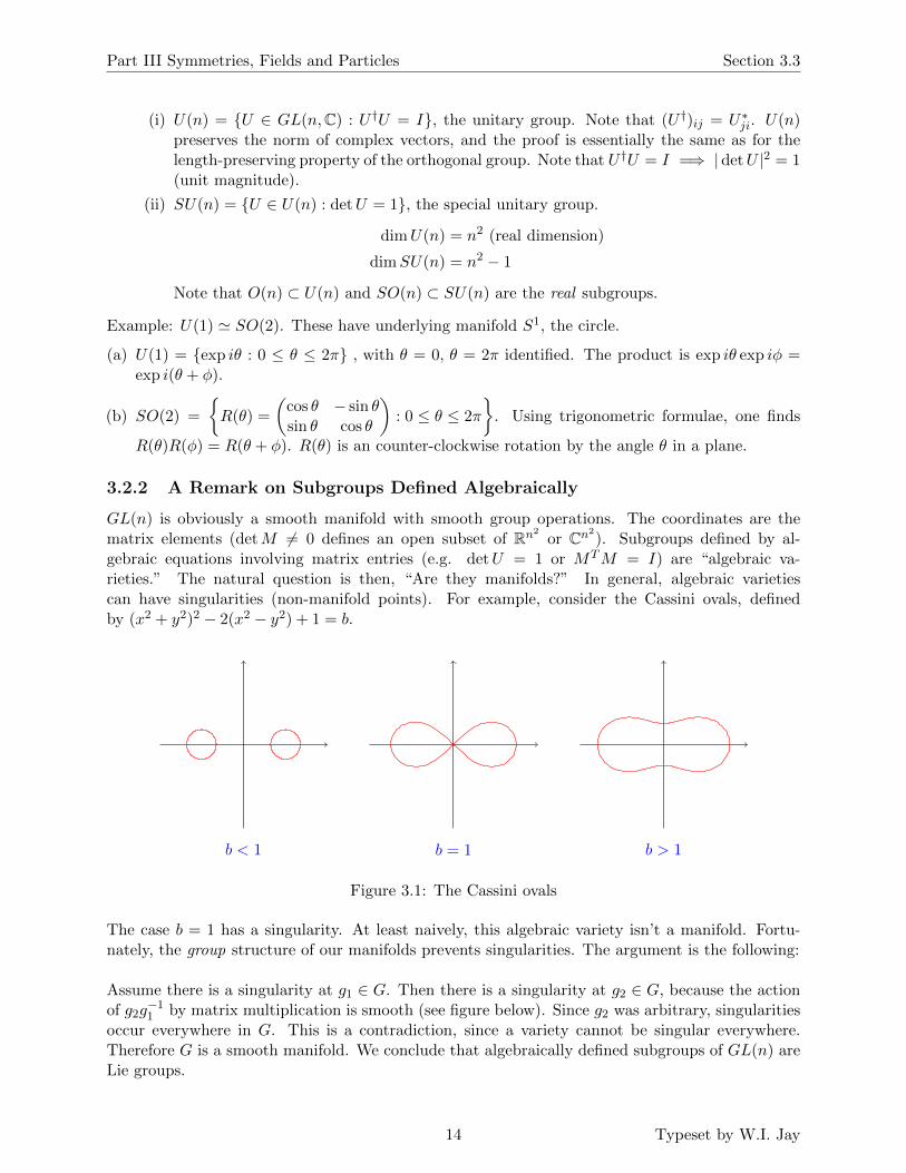
gebraic equations involving matrix entries (e.g. detU = 1 or MTM = I) are “algebraic va-rieties.” The natural question is then, “Are they manifolds?” In general, algebraic varietiescan have singularities (non-manifold points). For example, consider the Cassini ovals, definedby (x2 + y2)2 − 2(x2 − y2) + 1 = b.

b < 1 b = 1 b > 1

Figure 3.1: The Cassini ovals

The case b = 1 has a singularity. At least naively, this algebraic variety isn’t a manifold. Fortu-nately, the group structure of our manifolds prevents singularities. The argument is the following:

Assume there is a singularity at g1 ∈ G. Then there is a singularity at g2 ∈ G, because the actionof g2g

−11 by matrix multiplication is smooth (see figure below). Since g2 was arbitrary, singularities

occur everywhere in G. This is a contradiction, since a variety cannot be singular everywhere.Therefore G is a smooth manifold. We conclude that algebraically defined subgroups of GL(n) areLie groups.



!

g1

g2

g2g−11

smoothin bigger

group

3.3 Lie Algebras

The Lie algebra L(G) of a Lie group G is the tangent space to G at the identity I ∈ G. We studythe tangent space by differentiating curves in G. L(G) is a vector space of dimension dimG, withan algebraic structure called the Lie bracket. The algebraic structure of L(G) almost uniquelydetermines G. Group geometry thus reduces to algebraic calculations. This fact was useful to Lieand continues to be for physicists (and mathematicians, too). For two matrices X and Y , the Liebracket is [X,Y ] = XY −Y X, i.e., the commutator. We sometimes denote the Lie algebra of a Liegroup G using the lowercase Fraktur script g.

3.3.1 Lie Algebra of SO(2)

g(t) =

(cos f(t) − sin f(t)sin f(t) cos f(t)

)with f(0) = 0 is a curve in SO(2) through the identity. Differentiating with respect to t andevaluating at the origin gives:

dg

dt

∣∣∣t=0

=

(0 −11 0

)df

dt

∣∣∣t=0

.

For any f , this is a multiple of

(0 −11 0

). Thus

so(2) =

(0 −cc 0

): c ∈ R

.

Note that these matrices are not in SO(2); they’re in L(SO(2)), the tangent space at the identity.

3.3.2 Lie Algebra of SO(n)

Consider a curve R(t) ∈ SO(n) with R(0) = I. We require R(t)TR(t) = I. Differentiating withrespect to t, we find:

d

dt(R(t)TR(t)) = RT R+ RTR =

d

dtI = 0,∀t.



At t = 0, we have R = I, which gives the condition R+RT = 0. In other words, R is antisymmetric.Therefore we find that

L(SO(n)) = X : X +XT = 0= vector space of real antisymmetric n× n matrices.

dimL(SO(n)) =1

2︸︷︷︸symmetry

(n2 − n)︸︷︷︸diag = 0

=1

2n(n− 1)

Note that L(O(n)) = L(SO(n)) because an O(n) matrix R near the identity has detR = 1. Inother words, SO(n) is the part of O(n) that is connected to the identity.

!

!I

R(t) SO(n)

3.3.3 Lie algebra of SU(n) and U(n)

Let U(t) be a curve in SU(n) with U(0) = I. So U(t)†U(t) = I and detU(t) = 1. For small t, weassume that U(t) can be expanded as a power series: U(t) = I+tZ+ . . . . Z must be anti-hermitianso that U †U = I to first order in t. Then

U(t) =

1 + tZ11 tZ12 · · ·tZ21 1 + tZ22 · · ·

......

. . .

=⇒ detU = (1 + tZ11)(1 + tZ22) · · ·+O(t2)

= 1 + t(Z11 + Z22 + . . . ) +O(t2)

Thus we see that the condition detU = 1,∀t =⇒ TrZ = 0. Therefore

L(SU(n)) = Z : Z + Z† = 0 and TrZ = 0= n× n traceless anti-hermitian matrices

For U(n) there is no constraint on the phase of the determinant, so L(U(n)) = Z : Z +Z† = 0 =n× n anti-hermitian matrices.



3.3.4 General Structure of L(G) for a matrix group G

(1) Vector Space Structure:Suppose X1, X2 ∈ L(G). Then X1 = g1(t)|t=0, X2 = g2(t)|t=0 for curves g1(t), g2(t) ∈ G withg1(0) = g2(0) = I. Let g(t) = g1(λt)g2(µt), with λ, µ real. Then

d

dt(g1(λt)g2(µt))|t=0 = (λg1g2 + µg1g2)|t=0

= λg1 + µg2

= λX1 + µX2

∴ λX1 + µX2 ∈ L(G) =⇒ L(G) is a vector space.

Note that since the definition of the Lie algebra is the tangent space at the identity, thecomputation above really just shows that our definition is consistent with group composition,since the tangent space (at any point on any manifold) is a vector space.

(2) Bracket on L(G):We’ll now use more of the group structure. Let g1(t) , g2(t) be curves in G passing through Iat t = 0

g1(t) = I + tX1 + t2W1 + . . .

g2(t) = I + tX2 + t2W2 + . . .

Computing products, we find:

g1(t)g2(t) = I + t(X1 +X2) + t2(X1X2 +W1 +W2) +O(t3)

g2(t)g1(t) = I + t(X2 +X1) + t2(X2X1 +W2 +W1) +O(t3)

Define h(t) = g1(t)−1g2(t)−1g1(t)g2(t) or equivalently g1(t)g2(t) = g2(t)g1(t)h(t). h(t) is a curvein G. We see that

h(t) = I + t2[X1, X2] + . . . , (3.1)

where [X1, X2] = X1X2−X2X1. If we reparametrize according to t2 = s, we see that h(s) is acurve (for s ≥ 0) such that h(0) = I with tangent vector [X1, X2] ∈ L(G). Thus L(G) is closedunder the bracket operation. (h(t) has higher order terms at order t3 etc, and hence at orders3/2, but we only need h(s) to have a first derivative, so that’s no problem.)

Comment: Non-zero brackets are a measure of the non-commutativity of G. If G is abelian,h(t) = I ∀t, so L(G) has trivial brackets.

Lemma 3.3.1. If G is 1-dimensional, L(G) has trivial brackets.

Proof. L(G) = cX : c ∈ R for some fixed matrix X. [cX, c′X] = cc′[X,X] = 0.

The only connected 1-dimensional Lie groups are S1 and R.

(3) Antisymmetry and Jacobi Identity:The matrix bracket has the following general properties

(a) Antisymmetry [X,Y ] = −[Y,X]



(b) Jacobi identity: [[X,Y ], Z] + [[Y,Z], X] + [[Z,X], Y ] = 0 (prove this by expanding out).

Remark: An abstract Lie algebra L is a vector space with a bracket [ , ] : L×L→ L linearin both entries, satisfying antisymmetry and the Jacobi identity (cf. Humphreys, Intro.Lie Alg. and Rep. Thy.)

(4) Basis and Structure Constants:Let Ti be a basis for L(G). Define structure constants by [Ti, Tj ] ≡ cijkTk. Antisymmetrysays cijk = −cjik ⇔ c(ij)k = 0. Now computing the nested brackets gives:

[[Ti, Tj ], Tk] = cijl[Tl, Tk] = cijlclkmTm

[[Tj , Tk], Ti] = cjklclimTm

[[Tk, Ti], Tj ] = ckilcljmTm

Jacobi identity =⇒ cijlclkm + cjklclim + ckilcljm = 0

3.3.5 SU(2) and SO(3): The Basic Non-abelian Lie Groups

We begin by comparing the Lie algebras of SU(2) and SO(3), su(2) and so(3).

su(2) = 2× 2 traceless, anti-hermitian matrices: A basis is given in terms of the Pauli matrices:

Ta = −1

2iσa.

Here the σa are the (hermitian) Pauli matrices:

σ1 =

(0 11 0

), σ2 =

(0 −ii 0

), σ3 =

(1 00 −1

).

Recall the property of the Pauli matrices: σaσb = δabI + iεabcσc. Using this, one finds:

[Ta, Tb] = −1

4(σaσb − σbσa)

= −1

4(iεabcσc − iεbacσc)

= − i2εabcσc = εabcTc

=⇒ [Ta, Tb] = εabcTc

so(3) = 3× 3 antisymmetric real matrices: A basis for so(3) is given by:

T1 =

0 0 00 0 −10 1 0

, T2 =

0 0 10 0 0−1 0 0

, T3 =

0 −1 01 0 00 0 0

.

In other words, (Ta)bc = −εabc. Then [Ta, Tb] = εabcTc, as for su(2). So su(2) ' so(3). Thereforewe expect the groups SU(2) and SO(3) to be similar.

SU(2): U †U = I and detU = 1 imply that U has the form (cf. Example Sheet 1, Problem 6)U = a0I + i~a · ~σ with (a0,~a) real and a2

0 + ~a · ~a = 1. So the manifold of SU(2) is

SU(2) = S3 = unit sphere in R4



SO(3): A rotation is specified by an axis of rotation n (i.e. a unit vector ∈ R3) and by an angleof rotation ψ ∈ [0, π]. (A rotation by a larger angle is thought of as a rotation about −n.) Wecombine these into a 3-vector ψn ∈ ball of radius π ⊂ R3. Note that a rotation by π about n isequivalent to a rotation by π about −n. Thus opposite points on the boundary are identified, andconsequently the manifold SO(3) does not actually have a boundary.

SO(3) = ball in R3 of radius π with opposite points on boundary identified

! !

R3

π

3.3.6 The Isomorphism SO(3) ' SU(2)/Z2

SU(2) has a center Z(SU(2)) = Z2 = I,−I. If U = a0I+i~a·~σ, then (−I)U = −U = −a0I−i~a·~σ.Thus SU(2)/Z2 = S3 with antipodal points U,−U identified.

! !

R4

~a

a0 · ·

· ·−I

I

−U

U

S3 = SU(2)

∴ SU(2)/Z2 = upper half of S3 (a0 ≥ 0) with opposite points of equator S2 identified= curved version of SO(3).

! !

ψ

Note that the “curvature” is immaterial to the group or manifold structure. There is an explicitcorrespondence U ∈ SU(2) 7→ R(U) ∈ SO(3) with R(−U) = R(U), where U = cos α2 I + i sin α

2 n ·~σ 7→ R(U) = rotation by α about n.

3.4 Lie Group – Lie Algebra Relation

3.4.1 Tangent space to G at general element g

Let G be a matrix Lie group and g(t) ∈ G a curve. dgdt ≡ g is the tangent (matrix) at g(t) and

g(t + ε) = g(t) + εg(t) + O(ε2), where ε is infinitesimal. We can also write g(t + ε) as a product



in G: g(t + ε) = g(t)h(ε), where h(ε) = I + εX + O(ε2) for some X(t) ∈ L(G). h(ε) is the groupelement that generates the translation t 7→ t+ ε.! !

G

g(t)

g(t)

Then I + εX(t) = h(ε) = g(t)−1g(t + ε) = g(t)−1(g(t) + εg(t)) = I + εg(t)−1g(t) to O(ε). SoX(t) = g(t)−1g(t). Thus:

g(t)−1g(t) ∈ L(G), ∀t. (3.2)

Similarly, by putting (a different) h(ε) on the left of g(t) we have g(t)g(t)−1 ∈ L(G) (in general6= g−1g). We see that the tangent space to G at g is not the Lie algebra L(G), but is mapped toL(G) by either left or right multiplication by g−1.Important remark: Suppose g(x1, x2, . . . , xk) is a G-valued function on Rk. Then ∂

∂xig ≡ ∂ig is in

the tangent space to G at g, so (∂ig)g−1 ∈ L(G) and g−1(∂ig) ∈ L(G). These formulae appear ingauge theory.We now consider the converse. Suppose X(t) ∈ L(G) is a given curve in the Lie algebra. We canwrite down the equation:

g(t)−1g(t) = X(t),

g(0) = I (could be the more general element g0).

This equation with an initial condition has a unique solution in G. The equation makes intuitivesense because the “velocity” g is always tangent to G. As a special case, consider X(t) = X =const. Then g = gX with g(0) = I. This equation has the solution g(t) = exp tX.

Proof. By definition

exp tX =∞∑n=0

1

n!(tX)n (3.3)

and this series converges for all t. Then

d

dt(exp tX) = X + tX2 +

1

2t2X3

= exp(tX)X

Thus the equation is satisfied and g(0) = I. Note also that g(t) = exp(tX) commutes with X, soalso solves the equation g = Xg.

Claim: The curve gX(t) = exp(tX) : −∞ < t <∞ is an abelian subgroup of G, generated by X.

Proof. Using the series definition of exp(tX) one can verify that

g(0) = I,

g(s)g(t) = g(t+ s) = g(s+ t) (by combining all terms at a given order in X),

g(t)−1 = g(−t)



gX(t) is isomorphic either to (R,+) if gX(t) = I only for t = 0 or to S1 if gX(t0) = I for somet0 6= 0 and not for all t.

We can gain a general insight from the above considerations. Set t = 1, and consider all X ∈ L(G).We have then found a map L(G) → G, given by X 7→ expX. This map is locally bijective (proofomitted), as all elements g ∈ G close to I can be expressed uniquely as expX for some small X.

! !

L(G)

exp

G

·I

Note that this map is not globally simple and in most cases not even one-to-one. For example,the map R 7→ S1 given by θ 7→ exp iθ ∈ z ∈ C : |z| = 1 is onto but not one-to-one, asexp i2πn = 1, ∀n ∈ Z.In general, the image of exp is not the whole group G, but rather the component connected to I in G.

Example: O(3) is disconnected

! !

exp(tX)O(3) = ∪

exp(X)·

· ProperRotations in

O(3)

Det(R) = +1R ∈ SO(3)

Det(R) = −1R ∈ O(3)

ImproperRotations inO(3)

So exp so(3) = exp o(3) = SO(3). Evidently improper rotations R cannot be expressed as expXwith X antisymmetric and real.

3.4.2 The Baker-Campbell-Hausdorff Formula

If group elements are expressed as expX, X ∈ L(G), can we calculate products? Remarkably, thereis a universal formula:

expX expY = expZ, where Z = X + Y +1

2[X,Y ] + higher, nested brackets.

This can be checked up to the order given by expanding out both sides. Finding the structure ofthe BCH formula to all orders, and proving its validity, is not trivial.We deduce that the Lie algebra, with its bracket structure, determines the group structure of Gnear I.


Chapter 4

Lie Group Actions: Orbits

A Lie group G can act in many ways on other objects.

Definition 6. An action of G on a manifoldM is a set of smooth maps g :M→M for all g ∈ G,consistent with the group composition g1(g2(m)) = (g1g2)(m) for all g1, g2 ∈ G and for all m ∈M.

Note: This is equivalent to a map G×M→M, assumed here to be smooth in both arguments.

Definition 7. The orbit of a point m ∈M is the set G(m) = g(m) : g ∈ G

Proposition 1. If m′ ∈ G(m), G(m) = G(m′)

Proof. m′ = g(m) =⇒ G(m′) = G(g(m)) = (Gg)(m) = G(m)

Theorem 4.0.1. M is a disjoint union of orbits of G

Proof. (Omitted.) Two orbits are either the same, as sets, or have no point in common.

Example. SO(n) acts on Rn. The orbits are the spheres Sn−1, labelled by the radius r. The origin~0 ∈ Rn is special, as its orbit is this single point.

4.1 Examples of Group Actions

Definition 8. The left action of G on G is defined by g : G→ G with g(g′) = gg′

Definition 9. The right action of G on G is defined by g : G→ G with g(g′) = g′g−1

Note that the right action uses the inverse of g; this is necessary so that the action satisfies thegroup composition law.

Definition 10. An action G×M→M is said to be transitive if M consists of one orbit.

Transitivity of the left and right actions on G. Let g′, g′′ ∈ G. g′ and g′′ are in the same left orbit,since g(g′) = g′′ when g = g′′g′−1. A similar argument applies for right orbits.

Definition 11. Conjugation by G on G is the action defined by g(g′) = gg′g−1, ∀g, g′ ∈ G

The orbit structure under conjugation is more interesting. In particular, one can show (cf. ExampleSheet 2, Problem 4) that for matrices “conjugation preserves eigenvalues.” Matrices with differenteigenvalues must be in distinct orbits. The idea is that conjugation amounts to a change of basisin a matrix Lie group. Note also that one orbit is the identity alone, since g(I) = gIg−1 = I, ∀g.

22


Definition 12. The combined action of G×G on G is defined by (g1, g2)(g′) = g1gg−12 .

Note that G1 × G2 = (g1, g2) : g1 ∈ G1, g2 ∈ G2 with the product given by (g1, g2) ? (g′1, g′2) =

(g1g′1, g2g

′2) and identity (I1, I2).

Example. The actions of SU(2) on SU(2).Recall that we can express g ∈ SU(2) as g = a0I + i~a · ~σ with the constraint a2

0 + ~a · ~a = 1.(One way to see this parametrization is to think of SU(2) as the subgroup of the quaternions Hwith unit length.) This parametrization leads us to understand SU(2) to be S3 as a manifold. Ifg = a0I + i~a · ~σ and g′ = b0I + i~b · ~σ, we can look at the left action given by:

g(g′) ≡ gg′ = (a0b0 − ~a ·~b)I + i(a0~b+ ~ab0 − ~a×~b) · ~σ

≡ c0I + i~c · ~σ

(cf. Example Sheet 1, Problem 6 and Sheet 2, Problem 5 for details.) We see that (c0,~c) dependslinearly on (b0,~b) and c2

0 + ~c · ~c = b20 +~b ·~b = 1. Thus we see that the left action of g defines anelement of O(4) (depending on a0 and ~a).The identity I acts trivially, and SU(2) is connected, so the left action of g must be a proper rotation(a proper rotation is an element of SO(4) with det = +1). We deduce that SU(2)L ≤ SO(4),where the notation ≤ denotes a subgroup. Similarly, the right action gives a different subgroupSU(2)R ≤ SO(4) . In fact, the combined action of SU(2)L×SU(2)R gives every element of SO(4).

Theorem 4.1.1. SO(4) ' (SU(2)L × SU(2)R)/Z2

Proof. Omitted (cf. Example Sheet 2)

The subgroup Z2 consists of (I, I) and (−I,−I), since (g1, g2) and (−g1,−g2) act identically asSO(4) transformations. Because of the group structure given in the theorem, it follows that theLie algebra is given by so(4) = su(2)L ⊕ su(2)R.

4.2 The General Nature of an Orbit of G

Definition 13. Let G act on M transitively (single orbit). Let m ∈ M. The isotropy subgroup(or stabilizer) at m is the subset H of G that leaves m fixed:

H = h ∈ G : h(m) = m

We often write H(m) = m. H is a subgroup of G, because if h1(m) = m, h2(m) = m for h1, h2 ∈ H,then (h1h2)(m) = h1(h2(m)) = h1(m) = m. The inverses and identity are also in H.Using m as a base point forM, we can identify another point m′ with a coset of H. If m′ = g(m),then m′ = gH(m). The element m′ is identified not just with one element g that sends m to m′

but with the whole (left) coset gH. Thus we have

M' space of all cosets of H in G ≡ G/H

However, there is nothing special about the base point m. The isotropy group at m′ is H ′ = gHg−1,and this is structurally the same as H. We can check this:

H ′(m′) = gHg−1(m′) = gHg−1g(m) = gH(m) = g(m) = m′

Thus we regard G/H and G/H ′ as the same. This motivates the following definition:



Definition 14. Let G be a group acting smoothly and transitively on the manifoldM. M is saidto be a homogeneous space.

The critical part of the definition above is the transitivity: since there is just one orbit, all pointson M are “similar.”

Proposition 2. If H is a Lie subgroup of G and M is as above, then dimM = dimG− dimH.

We can check this statement near m. The tangent space to M is L(G)/L(H) (as vector spaces),as H acts trivially. If we find a vector space decomposition L(G) = L(H)⊕ Vm, with Vm a vectorspace complement to L(H) (could be orthogonal complement), then Vm can be identified with thetangent space to M at m.

Example. SO(3) acts transitively on S2, the unit sphere, since any point can be rotated into anyother point. The isotropy group at n is the SO(2) subgroup of SO(3) rotations about the axisthrough ~0 and n. Thus S2 = SO(3)/SO(2). Note that we usually choose the base point n so thatthe SO(2) rotations are about the x3-axis.

! !

o

S2

n


Chapter 5

Representations of Lie Groups

Definition 15. A representation D(G) of G is a linear group action v 7→ D(g)v of G on a vectorspace V , by invertible transformations. Let dimV = N . Then N is called the dimension of D andD(g) ∈ GL(N),∀g ∈ G.

Linearity says thatD(g)(αv1 + βv2) = αD(g)v1 + βD(g)v2

for v1, v2 ∈ V . To be a group action, D must satisfy

D(g1g2) = D(g1)D(g2)

We see that identity and inverses are particularly well-behaved: D(I) = IN and D(g−1) = D(g)−1.Note that in order to get explicit matrices we must choose a basis for V .

Definition 16. A representation is faithful if D(g) = IN only for g = I.

In a faithful representation distinct group elements are represented by distinct matrices. Note thata slightly more sophisticated definition would say that the homomorphism φ : G → GL(N) isinjective, i.e., that ker(φ) is trivial.

Example. Representations of the additive group R. We require D(α+ β) = D(α)D(β).

(a) D(α) = exp(kα), k ∈ R. This is faithful if k 6= 0.

(b) D(α) = exp(ikα), k ∈ R. This is not faithful as D(α) = 1 for α = 2πn/k.

(c) D(α) =

(cosα − sinαsinα cosα

). This representation has N = 2, and is not faithful.

(d) Let V = space of functions of x, an infinite-dimensional space. D is defined by (D(α)f)(x) =f(x− α). This is a simple example of an induced representation (see Chapter 12).

5.1 Types of Representation

Definition 17. LetG be a matrix Lie group with matrices of dimensionN . Then the representationD(g) = g is called the fundamental representation of the group, and is N -dimensional.

Definition 18. The representation of G that sets D(g) = IN ,∀g ∈ G (and for any N) is called thetrivial representation.

25


Definition 19. Let G be a matrix Lie group. Let V = L(G), the Lie algebra of G. The adjointrepresentation of G, denoted Ad, is the natural representation of G on L(G):

D(g)X ≡ (Ad g)X ≡ gXg−1, g ∈ G,X ∈ L(G)

Note that the adjoint representation Ad is the linearized version of the action of G on itself byconjugation. We do a couple of checks to make sure that we have a well-defined representation:

• Closure: gXg−1 ∈ L(G)There exists some curve g(t) = I+tX+. . . inG with tangentX at t = 0. Then g(t) = gg(t)g−1

is another curve in G and g(t) = I + tgXg−1 + . . . with tangent gXg−1 at t = 0, thusgXg−1 ∈ L(G).

• Ad is a representation:

(Ad g1g2)X = g1g2X(g1g2)−1

= g1g2Xg−12 g−1

1

= (Ad g1)(Ad g2)X

Note that we are thinking of L(G) as a real vector space, so Ad g ∈ GL(dimG,R). In fact, forU(n) and O(n), Ad g ∈ SO(dimG).

Definition 20. An N -dimensional representation D of G is said to be unitary if D(g) ∈ U(N), ∀g ∈G. If D is also real, then D(g) ∈ O(N), and the representation is said to be orthogonal.

Remark: Unitary representations are important in quantum mechanics and its various generaliza-tions because a symmetry group should preserve the norm of all wave functions.

Definition 21. Let D be a representation of G acting on the vector space V . Let A be a fixedinvertible transformation on V . Then we say that D(g) = AD(g)A−1 is an equivalent representationof G.

Note that equivalent representations are related by a change of basis of the vector space V .

Definition 22. Let D be a representation of G acting on V . D is reducible if there exists a proper,invariant subspace W ⊂ V , i.e., there exists a subspace W such that D(G)W ⊆ W . If no suchsubspace exists, then D is an irreducible representation, which we will sometimes call an “irrep”.

Note that D(G)W = W , since I ∈ G. (Also, for any g ∈ G, D(g)W = W , because D(g) isinvertible.)

Definition 23. A representation D is totally reducible if it can be decomposed into irreduciblepieces, i.e., if there exists a (possibly infinite) direct sum decomposition V = W1 ⊕W2 ⊕ . . .Wk

such that D(G)Wi = Wi and D restricted to Wi is an irrep.

In matrix language, for a totally reducible representation there exists a basis for V such that,simultaneously for all g, D(g) is block diagonal, taking the form:

D(g) =

D1(g) 0 · · · 0

0 D2(g) · · · 0...

.... . .

...0 0 0 Dk(g)

,

where the Di are each irreps. Wi consists of the column vectors which are zero in the subcolumnsacted on by Dj , j 6= i, and non-zero (generally) in the subcolumn acted on by Di.Note that it is usually not easy, nor even desirable, to find the basis that makes D block diagonal.One then needs other techniques to determine the decomposition of D into irreps.



Theorem 5.1.1. A finite-dimensional unitary representation is totally reducible.

Proof (sketch). For each invariant subspace W , the orthogonal complement W⊥ is also invariant,so V = W ⊕W⊥. Now reduce W and W⊥ until the process ends. Note that the process must endfor a finite-dimensional representation.(cf. Example Sheet 2, Problem 9 for more details)

The notions of irreducible representation, and total reducibility, are important, because vectorswithin Wi are actually related by G. The block diagonal form shows that vectors in Wi are notrelated by G to vectors in Wj (for j 6= i). If G is a symmetry acting on the Hilbert space V of allphysical states, then only physical states (particles!) within an irreducible subspace W have similarproperties.

Example. Let V = space of functions f of x with period 2π, i.e. f(x + 2π) = f(x). The circlegroup S1 acts on V by the representation (D(α)f)(x) = f(x− α), where 0 ≤ α ≤ 2π. This repre-sentation is infinite-dimensional.

The space Wn = f(x) = cneinx is a 1-dimensional invariant subspace for each n ∈ Z, be-

cause f(x − α) = cnein(x−α) = e−inαcne

inx. The 1-dimensional representation that occurs here isd(n)(α) = e−inα.

The Fourier series decomposition of a general function f

f(x) =

∞∑n=−∞

cneinx

exhibits the complete reducibility of V as

V = · · · ⊕W−2 ⊕W−1 ⊕W0 ⊕W1 ⊕W2 ⊕ · · ·

Each distinct 1-dimensional irrep of S1 occurs once in V .

There is a generalisation of this analysis for the action of SO(3) on functions defined on S2 (de-composition into spherical harmonics), and more generally for the action of any Lie group G onthe functions on any of its coset spaces G/H.


Chapter 6

Representations of Lie Algebras

By restricting a representation D of G to elements close to the identity I, we obtain the notion ofa representation of the Lie algebra L(G).

Definition 24. A representation d of L(G) acting on a vector space V is a linear action v 7→ d(X)v,with X ∈ L(G) and v ∈ V , satisfying

d([X,Y ]) = d(X)d(Y )− d(Y )d(X) = [d(X), d(Y )]

As with the case of groups, the dimension of the representation is dim d = N , where N is thedimension of the vector space V .

Example: For a matrix Lie algebra, the fundamental representation is d(X) = X. There alsoexists the trivial representation in which d(X) = 0, ∀X ∈ L(G).

A representation d of L(G) is called (anti)hermitian if d(X) is (anti)hermitian for all X ∈ L(G).

6.1 Representation of L(G) from a Representation of G

Let g(t) = I + tX + · · · ∈ G. Write D(g(t)) = IN + td(X) + . . . , which defines d(X). Then d is therepresentation of L(G) associated to D. We check now that the Lie bracket is preserved:As D is a representation of G

D(g−11 g−1

2 g1g2) = D(g1)−1D(g2)−1D(g1)D(g2).

Now set

g1(t) = I + tX1 + t2W1 + . . .

g2(t) = I + tX2 + t2W2 + . . .

g−11 (t) = I − tX1 − t2(W1 −X2

1 ) + . . .

g−12 (t) = I − tX2 − t2(W2 −X2

2 ) + . . .

After a brief computation very similar to the one leading to (3.1) we see that:

LHS = D(I + t2[X1, X2] + . . . ) = IN + t2d([X1, X2]) + . . .

RHS = IN + t2[d(X1), d(X2)] + . . .

and so we see the bracket is preserved.

28


Note: If D is a unitary representation of G, then d(X) is antihermitian for all X ∈ L(G). Why isthis true? If D(g) is unitary, then D(g) = I + td(X) and D(g)† = I + td(X)†, so D(g)D(g)† = Iimplies that d(X) + d(X)† = 0.

6.1.1 The adjoint representation of L(G)

The representation ad of L(G) is associated to Ad of G (both of these representations act on L(G),though one is a group representation and the other is a Lie algebra representation).Recall the adjoint representation (Ad g)Y = gY g−1, Y ∈ L(G). Set g(t) = I + tX, so g−1(t) =I − tX. Then

(Ad g)Y = (I + tX)Y (I − tX) +O(t2)

= Y − tY X + tXY +O(t2)

= Y + t[X,Y ] +O(t2)

≡ (I + t(adX))Y +O(t2)

Thus we see that(adX)Y = [X,Y ]

This is the adjoint representation of L(G) acting on itself. We can check easily (about three linesof computations) that ad[X,Y ] = [adX, adY ] using the Jacobi identity. (Act with both sides onZ ∈ L(G).)

6.2 Representation of G from a Representation of L(G)

Given g ∈ G, express g as expX for X ∈ L(G), then use the formula: D(expX) = exp(d(X)). Atleast locally (i.e., in a neighborhood of the identity), this defines a representation D of the groupG. How do we check this? We need to show that D “commutes appropriately” with exp:

D(expX)D(expY ) = D(expX expY )

(See Example Sheet 2, Problem 11). Summarizing, we have

(a) Always true: Rep. of G −→ Rep. of L(G)

(b) Mostly true: Rep. of L(G) −→ Rep. of G (works locally, but can encounter problems globally)

In practice (in physics) it is often easier use representations of L(G) rather than the correspondingrepresentations of G.Important questions now are: How can we classify and construct the irreps of L(G) and G? Whatare their dimensions? We start to answer this by looking at su(2)(= L(SU(2))). The results arevery helpful as most Lie algebras have several inequivalent su(2) subalgebras.

6.3 su(2): The Mathematics of Quantum Angular Momentum

We know that su(2) has the standard basis:Ta = −1

2iσa : a = 1, 2, 3



It is convenient for our current purposes to construct a new basis using (non-real) linear combina-tions:

h =

(12 00 −1

2

)=

1

2σ3 = iT3

e+ =

(0 10 0

)=

1

2(σ1 + iσ2) = iT1 − T2

e− =

(0 01 0

)=

1

2(σ1 − iσ2) = iT1 + T2

Note: This notation with h and e± appears in the text by Humphreys. h, e+, e− can be thought ofas analogous to the familiar operators J3, J+, J− in angular momentum theory.We have the brackets:

[h, e+] = e+

[h, e−] = −e−[e+, e−] = 2h

and one may also express these bracket relations in terms of the adjoint representation ad of su(2):

(adh)e+ = e+

(adh)e− = −e−(adh)h = 0

We see that we have diagonalized the operator adh, and e+, e−, h are eigenvectors. A maximalcommuting (i.e., abelian) subalgebra in su(2) is generated by h. The non-zero eigenvalues of adhare called roots.

! !

(0) 1−1

Figure 6.1: The root diagram for su(2)

6.3.1 Irreducible Representations of su(2)

The irreducible representations d(j) of su(2), with the label j (spin), are as follows:

j 0 12 1 3

2 . . .

dim 1 2 3 4 . . .

The representation d(j) acts on V (j), a vector space of dimension 2j + 1. We introduce a basis|j,m〉 for V (j), with m = j, j − 1, . . . ,−j + 1,−j (2j + 1 values). Then:

d(j)(h) |j,m〉 = m |j,m〉

d(j)(e−) |j,m〉 =√

(j −m+ 1)(j +m) |j,m− 1〉

d(j)(e+) |j,m− 1〉 =√

(j −m+ 1)(j +m) |j,m〉

One can show that [d(j)(e+), d(j)(e−)] = 2d(j)(h) etc. This irreducible representation is antihermi-tian, since d(j)(h)† = d(j)(h) and d(j)(e+)† = d(j)(e−), which tells us that d(j)(Ta) is an antihermitian



× × ××−j −j + 1 jj − 1· · ·

Figure 6.2: The weight diagram of d(j)

matrix. (Note: the basis h, e+, e− lives in the complexification su(2)C = su(2)⊗ C). The eigen-values of d(j)(h) are called weights and are real. For d(j), the weights are given by the labels m.

Some specific representations are: d(0) is the 1-dimensional trivial representation, d( 12

) is the fun-damental representation, and d(1) is the adjoint representation.

× ××

−1 0 1

Figure 6.3: The weight diagram of d(1), which is the same as the root diagram including zero

One can show that d(j) exponentiates to an irreducible representation D(j) of SU(2) for all j. AsL(SU(2)) and L(SO(3)) are the same, they have the same irreps d(j). However, only for integerj does the irrep d(j) exponentiate to an irrep of SO(3). One gets an SO(3) irrep because withinSU(2), for integer j, D(j)(−I) = I2j+1. (If j is half-integer, D(j)(−I) = −I2j+1, which forbids theZ2 quotient).

6.4 Tensor Products of Representations

Tensor products are one of the most useful constructions in physics. Using tensor products one cancombine representations of groups to produce a wide variety of physically interesting and usefulfurther representations. Let D(1)(g)αβ and D(2)(g)ab be representations of G acting on vectors

φ(1)β ∈ V

(1), φ(2)b ∈ V

(2). We define the tensor product D(1) ⊗D(2) acting on V (1) ⊗ V (2) by:

(D(1) ⊗D(2))(g)αa,βb ≡ D(1)(g)αβD(2)(g)ab

This acts on Φ ∈ V (1) ⊗ V (2) by:

Φαa 7→ Φ′αa = D(1)(g)αβD(2)(g)abΦβb

A special form of the tensor Φαa is the factorized form φ(1)α φ

(2)a , but this is not necessary (in other

words, not all tensors are the direct product of vectors). The dimension of the tensor productrepresentation is

dim(D(1) ⊗D(2)) = (dimD(1))(dimD(2))

6.4.1 The Representation of L(G) associated to D(1) ⊗D(2)

Let g ∈ G. Set g = I + tX. Then, up to order t,

D(1)(g)⊗D(2)(g) = (I + td(1)(X))⊗ (I + td(2)(X))

= I ⊗ I + t(d(1)(X)⊗ I + I ⊗ d(2)(X))

Thus the associated representation of L(G) is:

d(1⊗2) = d(1) ⊗ I + I ⊗ d(2)



We see that in the tensor product representation d(1⊗2), the eigenvalues of d(1) and d(2) add.Therefore the weights of d(1⊗2) are the sums of the weights of d(1) and d(2).

6.4.2 Tensor Products of su(2) Irreducible Representations

Let j denote the spin j irreducible representation d(j) of su(2). The tensor product j⊗j′ decomposesas

j ⊗ j′ = (j + j′)⊕ (j + j′ − 1)⊕ · · · ⊕ |j − j′| (6.1)

into a direct sum of irreducible representations. This formula, known as the Clebsch-Gordon series,is used for combining states of particles with spins j and j′. One can verify the formula above bycomparing weights on both sides (cf. Example Sheet 3, Problem 1).

Example:j = 1 has weights −1, 0, 1. j = 1

2 has weights −12 ,

12. Thus 1⊗1

2 has weights −32 ,−

12 ,−

12 ,

12 ,

12 ,

32 =

−32 ,−

12 ,

12 ,

32 ∪ −

12 ,

12. Thus 1⊗ 1

2 = 32 ⊕

12 .

= × ××× ××× ××

× ×⊗ =

× ×××

× ×⊕

Figure 6.4: A diagrammatic illustration of weights adding.

In Eq.(6.1) each state on the right |J,M〉 with |j − j′| ≤ J ≤ j + j′ can be expressed explicitly asa linear combination of states on the left:

|J,M〉 =∑m

cm |j,m〉 ⊗∣∣j′,M −m⟩

One writes more formally the coefficients cm as the Clebsch-Gordon coefficients cJjj′

Mmm′ , which(after a simple rescaling) are also known as the Wigner 3j symbols. They are non-vanishing onlyfor M = m+m′, which is just the statement that weights add. For more information, see Landauand Lifschitz, Quantum Mechanics, §106.

6.5 Roots and Weights for general L(G)

The following applies to the large class of Lie algebras called “semisimple”, which includes L(SU(n))and L(SO(n)). The definition is clarified in Section 8.2.

Definition 25. Let L(G) be a semisimple Lie algebra. A Cartan subalgebra is a subalgebra H ofL(G) such that:

(a) H is a maximal Abelian subalgebra of L(G)

(b) The adjoint representation ad of H is completely reducible.

Different Cartan subalgebras are related by conjugation by elements of G, so the Cartan subalgebrais essentially unique.

Definition 26. Let H be the Cartan subalgebra of L(G). The dimension of H is called the rankof G, and denoted by k.



Definition 27. Let hi : i = 1, 2, . . . , k be a basis of H. If L(G) has dimension n, one can finda standard basis h1, h2, . . . , hk; e1, e2, . . . , en−k, where each ep is a simultaneous eigenvector forall adhi (since these mutually commute). The simultaneous eigenvalues of adhi (collected into anon-zero k-component vector) are called roots.

The root diagram exhibits the roots in Cartesian k-space (simplest for k = 1 or k = 2). There aren− k roots.Now consider a representation d of L(G) acting on the N -dimensional vector space V . With hi asabove, the matrices d(hi) can be simultaneously diagonalized (since they again mutually commute).One can therefore find a basis for V consisting of simultaneous eigenvectors of d(hi). Let this basisbe ψ1, ψ2, . . . , ψN. For each basis element ψ we have

d(hi)ψ = miψ , where i = 1, ..., k

so ψ is the simultaneous eigenvector of d(hi) with the vector of eigenvalues ~m = (m1,m2, . . . ,mk).~m is called the weight vector, or simply weight, of ψ. The set of all weights, for ψ = ψ1, ψ2, . . . , ψN ,defines the set of weights for the representation d. The weights are k-vectors, and there are Nof them. Some of them can be identical (i.e., there can be “degeneracy”) and some can be zerovectors. (In the case of su(2), the weights were single numbers because the Cartan subalgebra wasspanned by a single element h.)The weight diagram of d exhibits the weights in Cartesian k-space (and the roots are sometimesshown at the same time). The most important weight diagrams are those of the irreps of L(G).The weights of a reducible representation d are just the union of the weights of all the irreps inthe decomposition of d. Weight diagrams can therefore be used to determine the decomposition ofa representation into irreps. (This is much easier than trying to find the block diagonal form, andalso easier than using characters.) There is also a (grand) weight diagram, which shows all possibleweights of all possible representations of L(G). The grand weight diagram is a lattice in k-space,called the weight lattice.The roots of L(G) are the non-zero weights of the adjoint representation ad of L(G). Thus

roots of L(G) ⊂ weight lattice of L(G)

We saw above that in a tensor product representation d(1⊗2) the eigenvalues of d(1) and d(2) add.In particular, each eigenvalue of d(1⊗2)(hi) is the sum of an eigenvalue of d(1)(hi) and an eigenvalueof d(2)(hi). The weights of d(1⊗2) are therefore obtained by adding a weight of d(1) and a weight ofd(2) in all possible ways. This will be illustrated in Chapter 9.


Chapter 7

Gauge Theories

Classical and quantum field theory is constructed from a Lagrangian density L which is gaugeinvariant and Lorentz invariant. The action is:

S =

∫R4

L d4x

A gauge theory has a Lie group G acting as a local symmetry, i.e., acting independently at eachspacetime point. Fields differing by a gauge transformation are physically the same.

7.1 Scalar Electrodynamics

Here the gauge group G is U(1), which is abelian. This theory describes the electromagnetic fieldinteracting with other electrically charged fields. The U(1) global symmetry leads to charge con-servation via Noether’s Theorem. Gauge symmetry is local and leads, additionally, to masslessphotons (see below).

We begin with the ungauged theory with a complex scalar field φ(x):

L =1

2∂µφ∂

µφ− U(φφ)

where U is a function (usually a polynomial) of |φ|2 = φφ. We use the convention ηµν =diag(+1,−1,−1,−1) for the Minkowski metric. So ∂µφ∂

µφ = ∂0φ∂0φ − ∇φ · ∇φ. This con-vention gives us a positive kinetic term (involving time derivatives) in L.

L is Lorentz invariant and invariant under the global U(1) symmetry φ 7→ eiαφ, φ 7→ e−iαφ. Toobtain a U(1) gauge theory, L must also be invariant under

φ(x) 7→ eiα(x)φ(x) (7.1)

where α(x) is an arbitrary, smooth real function. The U(φφ) term is gauge invariant as it stands,but the derivative terms cause a problem. The way to solve this is to introduce a new field, thereal gauge potential aµ(x), and the gauge covariant derivative of φ:

Dµφ = ∂µφ− iaµφ

(In this definition of Dµ we have set the coupling to unity.) We postulate that under the gaugetransformation (7.1) the gauge potential transforms according to:

aµ(x) 7→ aµ(x) + ∂µα(x)

34


With these definitions, we see that Dµφ transforms in the same way as φ (“covariantly” with φ):

Dµφ 7→ ∂µ(eiαφ)− i(aµ + ∂µα)(eiαφ)

= i(∂µα)eiαφ+ eiα∂µφ− iaµeiαφ− i(∂µα)eiαφ

= eiα(∂µφ− iaµφ)

= eiαDµφ

Similarly, the covariant derivative of φ is Dµφ = Dµφ = ∂µφ+ iaµφ, and so

Dµφ 7→ e−iαDµφ

under the gauge transformation. With these modifications, DµφDµφ is gauge invariant and Lorentz

invariant.The field aµ is also dynamical, and so we need its derivatives in L. The electromagnetic field tensorfµν = ∂µaν − ∂νaµ appears in L. We can easily verify its gauge invariance:

fµν 7→ ∂µ(aν + ∂να)− ∂ν(aµ + ∂µα)

= ∂µaν − ∂νaµ , by symmetry of partial derivatives

= fµν

We now combine these ingredients to construct a Lagrangian density for scalar electrodynamics:

L = −1

4fµνf

µν +1

2DµφD

µφ− U(φφ).

In order to understand the signs, we separate this equation into time and space parts. Recall:ei = f0i so ~e = ∂0~a −∇a0, and bk = 1

2εijkfij so ~b = ∇ × ~a, where ~e and ~b are the electric andmagnetic fields. Using this notation, we find

L = −1

4(−2~e · ~e+ 2~b ·~b) +

1

2D0φD0φ−

1

2~Dφ · ~Dφ− U(φφ)

=1

2~e · ~e+

1

2D0φD0φ︸︷︷︸

“Kinetic Terms”

−1

2~b ·~b− 1

2~Dφ · ~Dφ− U(φφ)︸︷︷︸

“Potential Terms”

This is a “natural Lagrangian density” in the sense that it takes the form L = T − V , where Tis quadratic in time derivatives. However, a0 is not dynamical. For completeness, we give theEuler-Lagrange equations, though their derivation is not a part of this course:

DµDµφ = −2U ′(φφ)φ

∂µfµν = − i

2(φDνφ− φDνφ)

where U ′ is the derivative of U with respect to its argument φφ.

Note: These are second-order evolution equations for φ,~a. The ν = 0 component is rather different(Gauss’ law...).



7.1.1 Field Tensor from Covariant Derivatives

[Dµ, Dν ]φ = (∂µ − iaµ)(∂ν − iaν)φ− (µ↔ ν)

= (∂µ − iaµ)(∂νφ− iaνφ)− (µ↔ ν)

=∂µ∂νφ− i(∂µaν)φ−iaν∂µφ−iaµ∂νφ−aµaνφ− (µ↔ ν)

= −i(∂µaν − ∂νaµ)φ

= −ifµνφ

So we see that the field tensor arises as a commutator of covariant derivatives.

7.2 A Non-Abelian Gauge Theory: Scalar Yang-Mills Theory

We now extend this formalism to a general gauge group G. We fix G = U(n) or some Lie subgroupof U(n) (e.g., SU(n), SO(n), . . . ). We introduce the fundamental scalar field

Φ(x) =

Φ1(x)...

Φn(x)

which has n complex components. As before, we can consider the global action of G

Φ(x) 7→ gΦ(x)

where g ∈ G is independent of x. However, we will require our theory to be invariant under gaugetransformations

Φ(x) 7→ g(x)Φ(x)

where g ∈ G depends on spacetime location. As previously, this inspires us to introduce the covariantderivative

DµΦ = (∂µ +Aµ)Φ,

with gauge potential Aµ(x) ∈ L(G). In particular, Aµ (as a member of the Lie algebra of U(n))is an n × n antihermitian matrix. Although there are certain geometric motivations, we postulatethat Aµ gauge transforms as:

Aµ 7→ gAµg−1 − (∂µg)g−1

Remark. Earlier (see the discussion leading to (3.2)) we discussed why expressions of the formg−1(∂µg) and (∂µg)g−1 are elements of the Lie algebra L(G). In our discussion of the adjointrepresentation of G, we also found that (Ad g)X = gXg−1 ∈ L(G) where g ∈ G and X ∈ L(G). SoAµ remains in L(G) after a gauge transformation.

Remark. This definition for the transformation of the gauge potential Aµ is consistent with ourprevious postulate for the transformation law in the abelian case of scalar electrodynamics. There,−iaµ 7→ g(−iaµ)g−1 − (∂µg)g−1 = −iaµ − i∂µα when g(x) = eiα(x), so aµ 7→ aµ + ∂µα.

We see that DµΦ transforms covariantly with Φ:

DµΦ = (∂µ +Aµ)Φ 7→ (∂µ + gAµg−1 − (∂µg)g−1)gΦ

=(∂µg)Φ + g(∂µΦ) + gAµΦ−(∂µg)Φ

= g(∂µΦ +AµΦ)

= gDµΦ



We now look for the Yang-Mills field tensor by examining the commutator of covariant derivatives:

[Dµ, Dν ]Φ = (∂µ +Aµ)(∂ν +Aν)Φ− (µ↔ ν)

= ∂µ∂νΦ +Aµ∂νΦ + ∂µ(AνΦ) +AµAνΦ− (µ↔ ν)

=∂µ∂νΦ +XXXXAµ∂νΦ + ∂µAνΦ +XXXXAν∂µΦ +AµAνΦ− (µ↔ ν)

= (∂µAν − ∂νAµ + [Aµ, Aν ])Φ

= FµνΦ

so we define Fµν ≡ ∂µAν − ∂νAµ + [Aµ, Aν ] as the field tensor in the non-abelian case.

Note: Fµν ∈ L(G) and Fµν = −Fνµ. The final term in Fµν can be interpreted abstractly as the Liebracket and not simply as the matrix commutator.

Proposition 3. Under a gauge transformation g(x), Fµν 7→ gFµνg−1.

Proof. [Dµ, Dν ]Φ 7→ g[Dµ, Dν ]Φ = gFµνΦ = (gFµνg−1)(gΦ). Thus we see that Fµν 7→ gFµνg

−1.

Remark. One can also compute this directly by gauge transforming Aµ, but the calculation islonger.

7.2.1 Lagrangian Density

For the Yang-Mills gauge potential Aµ coupled to the scalar Φ, the Lagrangian density is given by:

L =1

4Tr(FµνF

µν) +1

2(DµΦ)†DµΦ− U(Φ†Φ).

Lorentz invariance of L is clear, since all the Lorentz indices are contracted using the Minkowskimetric. However we still need to check gauge invariance:

Φ 7→ gΦ

Φ† 7→ Φ†g† = Φ†g−1 , since we’re in U(n)

∴ Φ†Φ 7→ Φ†g−1gΦ = Φ†Φ,

so U(Φ†Φ) is invariant. Since DµΦ transforms as Φ, the same argument applies to the second termin L. For the first term we see:

Tr(FµνFµν) 7→ Tr(gFµνg

−1gFµνg−1)

= Tr(FµνFµνg−1g) , since Tr is invariant under cyclic permutations

= Tr(FµνFµν)

Thus, the Lagrangian density is gauge invariant, and so is the action.

From the covariant derivative DµΦ = (∂µ+Aµ)Φ and the field tensor Fµν = ∂µAν−∂νAµ+[Aµ, Aν ]we see that the kinetic terms in the Lagrangian density are:

−1

2Tr(F0iF0i) +

1

2(D0Φ)†D0Φ

As F0i is an antihermitian matrix, −12 Tr(F0iF0i) is positive. Why is this true? If X is antihermitian,

TrX2 = XαβXβα = −XαβX∗αβ = −

∑α,β

|Xαβ|2

Hence all kinetic terms are positive. This is a consequence of the gauge group G being unitary (soelements of its Lie algebra are antihermitian).



7.2.2 Adjoint Covariant Derivative

Not all fields transform as Φ 7→ gΦ under gauge transformations. We could also have an adjointscalar field Ψ ∈ L(G) transforming as Ψ 7→ gΨg−1 (This looks like the transformation of Fµν .) Inthis case, the covariant derivative is:

DµΨ = ∂µΨ + [Aµ,Ψ]

To check this, one substitutes the transformation laws Ψ 7→ gΨg−1 and Aµ 7→ gAµg−1 − (∂µg)g−1

for the scalar field and gauge potential, respectively, into the proposed formula. One then sees aftera few lines of computation that the covariant derivative transforms as Ψ, i.e., DµΨ 7→ g(DµΨ)g−1.

7.2.3 General Covariant Derivative

Abstractly, we write Dµ = ∂µ+Aµ, where Aµ ∈ L(G) and [Dµ, Dν ] = Fµν = ∂µAν−∂νAµ+[Aµ, Aν ].In order to act concretely, we need a field Φ ∈ V (V is a vector space) and a representation Dof G acting on V . (Note that since D in this chapter denotes a covariant derivative we use Dfor a representation.) Then under gauge transformations the field transforms as Φ 7→ D(g)Φ andDµΦ = ∂µΦ + d(Aµ)Φ, where d is the representation of L(G) associated to D.

Claim: DµΦ transforms like Φ under gauge transformations.

Proof. We know Φ 7→ D(g)Φ and d(Aµ) 7→ D(g)d(Aµ)D(g−1)− (∂µD(g))D(g−1) Thus:

DµΦ = ∂µΦ + d(Aµ)Φ 7→ ∂µ(D(g)Φ) + (D(g)d(Aµ)D(g−1)− (∂µD(g))D(g−1))D(g)Φ

=(∂µD(g))Φ +D(g)(∂µΦ) +D(g)d(Aµ)Φ−

(∂µD(g))Φ

= D(g)(∂µΦ + d(Aµ)Φ)

= D(g)DµΦ

Thus DµΦ transforms covariantly with Φ under gauge transformations.

7.2.4 The Field Equation of Pure Yang-Mills Theory

The field equation for pure Yang-Mills theory is:

∂µFµν + [Aµ, F

µν ] = 0

Remark: This is an equation for Aµ involving second-order derivatives. In Yang-Mills theory, Fµν

is a derived quantity, while Aµ is considered fundamental (contrast with electromagnetism). Wemay rewrite the field equation more compactly using the adjoint covariant derivative:

DµFµν = 0

7.2.5 Classical Vacuum

Naively, the classical vacuum is Aµ = 0. We can gauge transform this to Aµ = −(∂µg)g−1. This isa “pure gauge,” which is physically the same as the vacuum. The Yang-Mills field tensor vanishesin both the classical vacuum and the pure gauge transformed vacuum: Fµν = 0 for both Aµ = 0and Aµ = −(∂µg)g−1.



Proof.

Fµν = ∂µAν − ∂νAµ + [Aµ, Aν ]

= ∂µ(−(∂νg)g−1)− ∂ν(−(∂µg)g−1) + [−(∂µg)g−1,−(∂νg)g−1]

=XXXXXXX−(∂µ∂νg)g−1 − (∂νg)(∂µg

−1) +XXXXXX(∂ν∂µg)g−1 + (∂µg)(∂νg

−1) + (∂µg)g−1(∂νg)g−1 − (∂νg)g−1(∂µg)g−1

= (∂µg)[(∂νg−1) + g−1(∂νg)g−1]− (∂νg)[(∂µg

−1) + g−1(∂µg)g−1]

= (∂µg)[∂ν(g−1g)]g−1 − (∂νg)[∂µ(g−1g)]g−1

But g−1g = I = const, so ∂ν(g−1g) = 0. Thus Fµν = 0 in the pure gauge Aµ = −(∂µg)g−1.

If there is a fundamental scalar field Φ as well, then in the vacuum Φ = 0 (provided Φ = 0 minimizesthe potential U(Φ†Φ)), and DµΦ = 0.

7.3 A Very Brief Introduction to Mass and the Higgs Mechanism

Recall the Klein-Gordon theory for a scalar field φ is governed by the Lagrangian density:

L =1

2∂µφ∂

µφ− 1

2m2φ2

As shown in quantum field theory, the equation of motion is the Klein-Gordon equation:

∂µ∂µφ+m2φ = 0

This equation has wavelike solutions of the form φ = exp[i(ωt − ~k · ~x)] provided ω2 = |~k|2 + m2.Here m is the “mass parameter” of the field. Particles arise when the field is quantized. Particleenergy is given by E = ~ω; particle momentum is given by ~p = ~~k. Thus E2 = |~p|2 + (~m)2. So inunits where c = 1, the particle has mass ~m. In units where also ~ = 1 the mass is m.

7.3.1 Electrodynamics

We have the Lagrangian density L = −14fµνf

µν with fµν = ∂µaν − ∂νaµ. The Maxwell equationsays:

∂µfµν = 0 =⇒ ∂µ(∂µaν)− ∂ν(∂µa

µ) = 0

If we work in the Coulomb gauge, ∂iai = 0, i = 1, 2, 3, i.e., ∇·~a = 0, then ∂µaµ = ∂0a0. Let us take a

closer look at the ν = 0 equation ∂µ∂µa0−∂0(∂0a0) = (∂0∂0−∂i∂i)a0−∂0∂0a0 = 0 =⇒ ∇2a0 = 0.

Without any special boundary conditions or sources, the solution is evidently a0 = 0. The remain-ing equations are (∂µ∂

µ)ai = 0. These are three massless wave equations.

We see that polarization is transverse to momentum: If ai = εi exp[i(ωt − ~k · ~x)], then ω2 = |~k|2(massless!), and the gauge condition ∂iai = 0 tells us ~k · ~ε = 0. After quantization, the photon hasthe following properties:

• zero mass, so energy satisfies E = |~p|

• 2 (transverse) polarization states: ~ε ⊥ ~p

• non-vanishing momentum: ~p 6= 0



The last condition is because the ω = ~k = 0 wave, ai = εi, is pure gauge and has vanishing fieldtensor. So it is the vacuum.

The quantized particles of pure Yang-Mills theory are also massless, but confined. They are calledgluons in the SU(3) theory of quantum chromodynamics. This phenomenon is only partiallyunderstood.

7.3.2 Perturbative Effect of Interaction of EM Field with a Charged ScalarField

The scalar particle mass m is renormalized, thereby changing its value. The photon, however,remains massless. This result is complicated to prove. However, it may be understood as arisingfrom:

(a) No term of the form 12M

2aµaµ is allowed, because it wouldn’t be gauge invariant.

(b) A massive vector particle can have ~p = 0, and it then has three polarization states (i.e.,~ε · ~p = 0 doesn’t constrain ~ε if ~p = 0). However a continuous perturbation cannot change thenumber of polarization states.

7.3.3 Higgs Mechanism

The Higgs mechanism evades these two previous arguments. In scalar electrodynamics, the “pho-ton” can become massive. The abelian Higgs model has the Lagrangian density:

L = −1

4fµνf

µν +1

2DµφD

µφ+1

2µ2φφ− 1

4λ(φφ)2 (7.2)

Evidently, the potential is U = −12µ

2φφ+ 14λ(φφ)2 = −1

2µ2|φ|2 + 1

4λ|φ|4.

! !

U

Re(φ)

Im(φ)

! !

U

|φ|

Figure 7.1: The so-called “Mexican hat potential” (before shifting it up)

Often it is convenient to shift the potential up and write U = 14λ(|φ|2− v2)2, where µ2 = λv2. This

shift is by a constant value of 14λv

4, which has no effect on the field equations. The vacuum isbased around the classical field that minimizes the energy, and in particular minimizes U . It is notat φ = 0, but where |φ| = v. Further, the vacuum is degenerate (related by gauge transformations);it is a non-trivial orbit of the gauge group U(1). We call v the vacuum expectation value (vev) ofφ (or more accurately of |φ|). The simplest vacuum is φ = v, aµ = 0. We can gauge transformthis vacuum to φ = v exp iα(x), aµ = ∂µα. A natural question is then how this affects the twoarguments above that kept the photon massless.



(a′) There is now a mass term for aµ:

Part of 12DµφD

µφ is 12(−iaµφ)(−iaµφ) = 1

2aµaµ|φ|2. Close to the vacuum, this is 1

2v2aµa

µ +higher order terms. Thus the “photon” acquires mass v and gets the new name massive vectorboson.

Remark: The term we’ve singled out would, by itself, violate gauge invariance. However, theother terms present in the Lagrangian combine to preserve the gauge invariance.

(b′) The massive vector boson has three polarization states. We can impose the gauge condition

Im φ = 0, φ(x) = v + η(x)

where η(x) is real. We cannot simultaneously impose the Coulomb gauge. Thus the physicalparticles are:

• a massive vector boson with three states, and

• a real scalar particle H from the field η with one state.

Alternatively, in the Coulomb gauge, we need to allow φ(x) = exp[iβ(x)](v + η(x)) withβ(x), η(x) real. The third (longitudinal) polarization state of the vector boson now comesfrom β. For the mass of the Higgs particle H, look at the quadratic terms in η (with aµ = 0).

Lη =1

2∂µη∂

µη − 1

4λ((v + η)2 − v2)2 =

1

2∂µη∂

µη − λv2η2 + . . .

which we find from substituting φ(x) = v+η(x) into L. Thus we see that mH =√

2λv =√

2µ.

7.3.4 Higgs Mechanism in the Non-abelian Case

The Standard Model has electroweak gauge group G = U(2) and a scalar field Φ, which is a doubletof complex scalar fields. U(2) acts by the fundamental representation. The Higgs mechanism occursif Φ 6= 0 in the classical vacuum, i.e., if the minimum of the potential U(Φ†Φ) is on a non-trivialorbit of the gauge group G. We expect the orbit to have the form G/K for some subgroup K ≤ G.The gauge symmetry is still present, but the choice of a vev for Φ (which is just a choice of gauge)apparently breaks the G-symmetry. One says that the G-symmetry is spontaneously broken, whilethe K-symmetry (which leaves the vev fixed) remains unbroken. Massless gauge bosons remain forK. In the Standard Model, G = U(2),K = U(1), and as U(2) is a 4-dimensional Lie group, we get:

• 3 massive vector bosons W+,W−, Z

• 1 massless vector boson, the photon

• 1 real (electrically neutral) Higgs boson

The masses of the vector bosons and Higgs particle are unrelated, so the Higgs mass had to bedetermined experimentally.


Chapter 8

Quadratic Forms on Lie Algebras andthe Geometry of Lie Groups

8.1 Invariant Quadratic Forms

For a matrix Lie algebra L(G), we have the quadratic form L(G) × L(G) → C (symmetric innerproduct) given by:

(X,Y ) = Tr(XY )

where X,Y ∈ L(G). This quadratic form is G-invariant in the following sense:

(X,Y ) 7→ (gXg−1, gY g−1) = Tr(gXg−1gY g−1) = Tr(XY ) = (X,Y )

where g ∈ G. One can also use a different representation d of L(G) and define (X,Y )d =Tr(d(X) d(Y )), which is similarly invariant: (gXg−1, gY g−1)d = (X,Y )d. This is a result of thefollowing lemma:

Lemma 8.1.1. If d is a representation of L(G) associated to the representation D of G, thend(gXg−1) = D(g)d(X)D(g)−1.

Proof. For g′ ∈ GD(gg′g−1) = D(g)D(g′)D(g)−1

Now set g′ = I + tX with t small, and ignore terms of order t2. Then

D(gg′g−1) = D(g(I + tX)g−1)

= D(I + tgXg−1)

= I + td(gXg−1)

whereas

D(g)D(g′)D(g)−1 = D(g)(I + td(X))D(g)−1

= I + tD(g)d(X)D(g)−1

Comparing the terms of order t gives the result.

42


As a special case, we consider the adjoint representation of L(G), which gives rise to the so-calledKilling form:

κ(X,Y ) = Tr(adX adY )

The Killing form is real and is the most basic inner product, because every Lie algebra has anadjoint representation. In practice, these inner products are usually related. They differ by a con-stant multiple if L(G) is “simple” (to be made precise soon).

The infinitesimal version of the invariance above is the associativity property :

Claim: (X, [Y, Z])d = ([X,Y ], Z)d

Proof. (For the initial inner product in this section)Tr(X, [Y,Z]) = Tr(XY Z)− Tr(XZY ) = Tr(XY Z)− Tr(Y XZ) = Tr([X,Y ]Z)

What does this have to do with an infinitesimal version of the invariance under the conjugationX 7→ gXg−1? If we let g = I + tZ ∈ G with t infinitesimal, then we have to order t:

Tr(XY ) = Tr((1 + tZ)X(1− tZ)(1 + tZ)Y (1− tZ))

= Tr((X − t[X,Z])(Y + t[Z, Y ]))

= Tr(XY )− tTr([X,Z]Y ) + tTr(X[Z, Y ])

=⇒ Tr([X,Z]Y ) = Tr(X[Z, Y ])

which is just the associativity property.

8.2 Non-Degeneracy of the Killing Form

Let Ti be a basis for L(G). The Killing form becomes a symmetric matrix with components

κij = κ(Ti, Tj) = Tr(adTi adTj)

Now adTi is defined by (adTi)X = [Ti, X], where X ∈ L(G). Let X = XlTl (basis expansion).Then

(adTi)X = [Ti, XlTl] = Xl[Ti, Tl] = cilkXlTk =⇒ (adTi)kl = cilk

Although the indices look a bit strange in the final equality of the last line, they are in fact correct.Therefore we have Tr(adTi adTj) = (adTi)kl(adTj)lk = cilkcjkl. So the (ij)th component of theKilling form is given by:

κij = cilkcjkl

Example. For the standard basis of su(2), κab = εadcεbcd = −2δab. This is a non-degenerate Killingform.

Definition 28. The Killing form κij is non-degenerate if all of its eigenvalues are non-zero. Equiv-alently, detκij 6= 0 and κij is invertible, since detκij =

∏λi, where λi are the eigenvalues.

Definition 29. A Lie algebra L(G) is said to be semi-simple if its Killing form is non-degenerate.

Theorem 8.2.1. A semi-simple Lie algebra L(G) has a decomposition into mutually commutingsimple factors L(Gi) such that

L(G) = L(G1)⊕ L(G2)⊕ · · · ⊕ L(Gk)

and L(G) cannot be reduced further.



Proof. Omitted (but see Example Sheet 4, Problem 6 for some related details). The general ideais that a non-degenerate Killing form gives a way to build “orthogonal complements,” which leadsto a direct sum decomposition of the Lie algebra.

Fact: In the case of L(G) semi-simple, the associated group G has the structure

G = G1 ×G2 × · · · ×Gk/discrete group

where Gi are simple Lie groups. (Note: A simple Lie group is a connected, non-abelian Lie groupwith no (proper) normal Lie subgroups.)

8.3 Compactness

If κij is negative definite, L(G) is said to be of compact type. G is then a compact group (as atopological manifold). For example, SU(n) is simple and compact. In the case of L(G) of compacttype, we can find an adapted basis Ti such that κij = −µδij , for some constant µ > 0.

Then κ(Ti, [Tj , Tk]) = κ(Ti, cjklTl) = cjklκil = −µcjki, and κ([Ti, Tj ], Tk) = κ(cijlTl, Tk) = cijlκlk =−µcijk. Thus by the associativity property we have:

cijk = cjki = ckij = −cjik = −ckji = −cikj

In other words, the structure constants are totally antisymmetric in the adapted basis.

We can now clarify why gauge groups are chosen to be compact. If L(G) is of compact type thenthe Yang-Mills Lagrangian density

LYM = κ(FµνFµν)

is gauge invariant because of the G-invariance of κ, and has positive kinetic terms (remember theextra minus sign from lowering Lorentz indices). For a simple matrix group G, this density is apositive multiple of Tr(FµνF

µν). (Non-compact groups have Killing forms κ of mixed signature,which would lead to unphysical negative kinetic energy in some cases; as κ is not positive definite,we cannot just flip the sign.)

8.4 Universal Enveloping Algebra

In a matrix Lie algebra L(G), we can deal with a product XY (which isn’t necessarily in L(G)) aswell as the commutator [X,Y ] (which is in L(G)). In an abstract Lie algebra L, we can define theuniversal enveloping algebra (UEA) to be the formal span of 1, L, L⊗L,L⊗L⊗L, . . . , allowingsums and products of elements of L. The UEA is subject to the one rule: XY − Y X = [X,Y ], asdefined in L.

(a) In the UEA we see that there are new identities, e.g.

[X,Y Z] = XY Z − Y ZX = XY Z − Y XZ + Y XZ − Y ZX= [X,Y ]Z + Y [X,Z]

(b) We have

expX = 1 +X +1

2X2 + · · · ∈ UEA



Thus the connected component of G is in the UEA of L(G). (Note: This is a bit of a white lie,as the UEA technically only contains finite sums, while the definition of exp involves infinitesums. However, we assume that the idea may be extended in a more careful treatment toinclude a “formal completion of the UEA”.)

(c) There is an analogy between a UEA and the Dirac matrix algebra, which is the span ofI, γµ, γµγν , γµγνγσ, ... subject to the constraint γµγν + γνγµ = 2ηµνI.

One can extend an N -dimensional representation d of L to the UEA in the obvious way (replaceX by d(X) and 1 by IN ). All elements are now N × N matrices. Usually there are additionalidentities satisfied by the matrices d(X) which are not universal. It is important not to be deceivedby these. E.g. (σ1)2 = I2 for the Pauli matrix σ1 does not imply that (T1)2 is a multiple of 1 inthe UEA of L(SU(2)).

8.5 Casimir Elements

Let L(G) be a Lie algebra of simple (irreducible in the sense that it isn’t a direct sum of mutuallycommuting subalgebras) compact (κij negative definite) type with adapted basis Ti such thatκij = −δij . Here the basis elements are normalized so that µ = 1.

Definition 30. The universal (quadratic) Casimir element in the UEA is C =∑

i TiTi.

Lemma 8.5.1. [X,C] = 0 for all X ∈ L(G), i.e., the Casimir commutes with every element in theLie algebra:

Proof. It is sufficient to set X equal to the basis element Tj .

[Tj , C] =∑i

[Tj , TiTi]

=∑i

(Ti[Tj , Ti] + [Tj , Ti]Ti)

=∑i

(TicjikTk + cjikTkTi)

=∑i

cjik(TiTk + TkTi) = 0

where the last line follows because the antisymmetric structure constants (adapted basis) are con-tracted against a symmetric quantity.

It follows that the Casimir C is a central element (commutes with everything) in the UEA. How-ever, this does not mean that it is a fixed multiple of 1. (The UEA has as further central elementsall polynomials in C. It may have yet more independent central elements, higher Casimirs, butthese depend on the detailed form of L(G) and do not have a universal form.)

Consider now C in a representation d of L(G) of dimension N :

Cd =∑i

d(Ti)d(Ti),

where Cd is now an N ×N matrix. By the same proof as above, [d(X), Cd] = 0,∀X ∈ L(G).

Claim: If d is irreducible, then by Schur’s lemma Cd = cdIN .



Proof. Example Sheet 3, Exercise 7

Here the Casimir eigenvalue cd is a useful way to characterize the irreducible representation d.

Example. Consider the fundamental (j = 12) representation of su(2). The adapted basis is Ta =

− i2√

2σa (notice the factor of

√2). Then:

C(j= 12

) =∑a

(Ta)2 = −1

8

∑a

σ2a = −3

8I2.

Thus c(j= 12

) = −38 . More generally, consider the well-known angular momentum operators J1, J2, J3

from physics. They have the Casimir operator:

C = −1

2~J2 = −1

2(J2

1 + J22 + J2

3 )

Quoting a familiar result, the eigenvalue in the spin j irreducible representation is c(j) = −12j(j+1).

8.6 Metric on G

(Note: In what follows the assumption that G is a simple Lie group is non-essential, but with thisassumption the metric we find is unique up to a constant multiple. The assumption of compactnessgives a Riemannian metric. Otherwise we can wind up with a Lorentzian metric, for example.)

Suppose G is a simple matrix Lie group with Lie algebra of compact type. Let X,Y ∈ L(G) betangent vectors at I. Define (X,Y ) = −Tr(XY ). Up to a constant multiple, this is the uniquepositive definite quadratic form on L(G) which is also invariant under the action of conjugation onX,Y by G. We can use this quadratic form to define a Riemannian metric on G:

ds2 = −Tr((dg)g−1(dg)g−1

)(8.1)

where dg is an infinitesimal tangent element to G at g. By the argument used previously leadingto (3.2), we see that (dg)g−1 ∈ L(G). ds2 is interpreted as the squared length of dg.

! !

!

!

· Ig

g + dg

dg

Note: We must use g−1 to map dg back to the identity, where we can use the Lie algebra innerproduct ( , ).



If we’re near the identity, g = I and g + dg = I + dX, where dX is an infinitesimal element ofL(G). Then (dg)g−1 = dX and ds2 = −Tr(dXdX).

! !

!

!

I

I + dX

dX

A natural question to ask is how this metric behaves under the left and right actions of G. If

g 7→ g1gg−12 , dg 7→ g1dgg

−12

with g1, g2 constant, then dgg−1 7→ g1dgg−1g−1

1 and

ds2 7→ −Tr(g1dgg−1g−1

1 g1dgg−1g−1

1 ) = −Tr(dgg−1dgg−1) = ds2

(dg transforms like g because it is the difference of two infinitesimally separated group elements.)Thus we’ve found that our metric is invariant under the action of G × G on G; such a metric issometimes called a bi-invariant metric. This metric is highly symmetric and unique up to a scalarmultiple.

Note: The high degree of symmetry is clear from the above discussion, but we haven’t shownuniqueness.

8.7 Kinetic Energy and Geodesic Motion

For a particle moving on G along the trajectory g(t), we can define the kinetic energy:

T = −Tr(gg−1gg−1

), with g ≡ dg/dt

and the action:

S = −t1∫t0

Tr(gg−1gg−1

)dt

The stationarity condition δS!

= 0 gives ddt(g

−1g) = 0 as the equation of motion (Example Sheet3, Problem 9). As the action is defined using the metric on G, and is purely kinetic, solutionscorrespond to motion along geodesics at constant speed.

If we integrate the equation of motion once with respect to time, we see:

g−1g = X0 = const. ∈ L(G)



The function g(t) = exp(tX0) is a solution with g(0) = I. It is easy to check this if one recallsthat exp(±tX0) and X0 commute. The general solution is a left translation of this special solutiongiven by g(t) = g0 exp(tX0), where X0 ∈ L(G) , g0 ∈ G are both constant. We can check that thisdoes in fact solve the differential equation:

g(t) = g0X0 exp(tX0), so

g−1g = (g0 exp(tX0))−1g0X0 exp(tX0)

= exp(−tX0)g−10 g0X0 exp(tX0)

= X0

Remark: Geodesic motion possesses enough symmetry in this case that it is completely integrable.

8.8 SU(2) Metric and Volume Form

Recall (from example sheets) the following parametrizations of SU(2) as a 3-sphere:

U =

(a0 + ia3 ia1 + a2

ia1 − a2 a0 − ia3

), with a2

0 + ~a · ~a = 1

U =

(α β−β∗ α∗

), with |α|2 + |β|2 = 1

(These parametrizations are really the same and in fact give a quick way to recall explicit forms forthe Pauli matrices.) We know that an SU(2)×SU(2) invariant metric on SU(2) is SO(4) invariant.This fact follows because we showed that so(4) = su(2)⊕ su(2). The bi-invariant metric on SU(2)is therefore the round metric on S3:

ds2 = da20 + d~a · d~a, restricted to S3

ds2 = dαdα∗ + dβdβ∗, with the restriction |α|2 + |β|2 = 1

Exercise: (Example Sheet 4, Problem 2) Show that ds2 = −12 Tr

((dU)U−1(dU)U−1

).

8.8.1 Euler Angle Parametrization

Let α = cos θ2 exp(i2(φ+ ψ)

), β = sin θ

2 exp(i2(−φ+ ψ)

), with θ ∈ [0, π], φ ∈ [0, 2π], ψ ∈ [0, 4π]. If

one computes the differentials dα and dβ, one finds after a few lines of algebra that:

ds2 = dαdα∗ + dβdβ∗ =1

4(dθ2 + dφ2 + dψ2 + 2 cos θ dφdψ)

This is the round metric on S3 in terms of Euler angles (cf. Landau and Lifschitz Vol. I for morediscussion). The metric tensor is therefore:

gµν =1

4

1 0 00 1 cos θ0 cos θ 1

The volume form is dV =

√det gµν dθdφdψ = 1

8 sin θ dθdφdψ. Using it, we can compute the totalvolume of SU(2):

V =1

8

∫sin θ dθdφdψ = 2π2

(Note: The volume form is useful in gauge theory quantization. Like the metric, the volume formis bi-invariant. In general a volume form on a differentiable manifold M is a nowhere-vanishingdifferential form of top degree. On a manifold M of dimn, a volume form is an n-form, a sectionof the line bundle Ωn(M) = Λn(T ∗M).)


Chapter 9

SU(3) and its Representations

9.1 Roots

Recall the brackets of the SU(2) Lie algebra su(2):

[h, e+] = e+

[h, e−] = −e−[e+, e−] = 2h

where e±, h is a basis for (complexified) su(2). Recall that su(3) consists of traceless, anti-hermitian 3×3 matrices. A convenient basis (and one with similarities to the basis for su(2) above)for the complexified su(3) (i.e., for su(3)⊗ C) is:

eα =

0 1 00 0 00 0 0

, e−α =

0 0 01 0 00 0 0

, eβ =

0 0 00 0 10 0 0

e−β =

0 0 00 0 00 1 0

, eγ =

0 0 10 0 00 0 0

, e−γ =

0 0 00 0 01 0 0

and two in the span of

hα =

1/2 0 00 −1/2 00 0 0

, hβ =

0 0 00 1/2 00 0 −1/2

, hγ =

1/2 0 00 0 00 0 −1/2

With these definitions, we have the following commutation relations (among others):

[hα, eα] = eα

[hα, e−α] = −e−α[eα, e−α] = 2hα

These are precisely the commutation relations fulfilled by su(2). Thus eα, e−α, hα is the basis ofan su(2) subalgebra, and similarly for β, γ. However, hα + hβ = hγ , so these subalgebras are notlinearly independent. We can choose a basis for the diagonal matrices:

h1 =

1/2 0 00 −1/2 00 0 0

, h2 =1√3

1/2 0 00 1/2 00 0 −1

49


They are orthonormal in the sense: Tr(h 21 ) = Tr(h 2

2 ) = 1/2 and Tr(h1h2) = 0. We write ~h =(h1, h2) as a vector and define:

~α = (1, 0)

~β = (−1/2,√

3/2)

~γ = (1/2,√

3/2)

Using this notation we see:

~α · ~h = (1, 0) · (h1, h2) = h1 = hα

~β · ~h = (−1/2,√

3/2) · (h1, h2) = −1/2h1 +√

3/2h2

=

−1/4 0 00 1/4 00 0 0

+

1/4 0 00 1/4 00 0 −1/2

= hβ

~γ · ~h = (1/2,√

3/2) · (h1, h2) = 1/2h1 +√

3/2h2

=

1/4 0 00 −1/4 00 0 0

+

1/4 0 00 1/4 00 0 −1/2

= hγ .

We can verify, and write compactly:

[~h, eα] = (ad~h)eα = (1, 0)eα = ~αeα

[~h, eβ] = (ad~h)eβ =

(−1

2,

√3

2

)eβ = ~βeβ

[~h, eγ ] = (ad~h)eγ =

(1

2,

√3

2

)eγ = ~γeγ

Note that [hα, eα] = [~α · ~h, eα] = (~α · ~α)eα = eα as |~α| = 1. In other words, all of this notation isconsistent. This notation leads to the root diagram of su(3):

-~α ~α

~β

-~β-~γ

~γ

···

·

·

·

Figure 9.1: The root diagram of L(SU(3))



±~α,±~β,±~γ are the roots of su(3). (In this case they are of unit length.) The negative roots areincluded because:

[e−α, eα] = −2hα = 2h−α = 2(−~α) · ~h

and so on. su(3) is said to have rank 2. The rank is the dimension of the maximal commutingsubalgebra (the Cartan subalgebra, or CSA), which is here spanned by h1 and h2. The root diagramis two-dimensional. su(3) has three (special) su(2) subalgebras, one for each pair ±α,±β,±γ. Thereare also further brackets that we have not yet given, e.g.,

[eα, eα] = 0

[eα, eβ] = eγ

[eα, eγ ] = 0

and so on . . .

Remark. We show below that these roots are consistent with our previous definition of roots asnon-zero eigenvalues of the Cartan subalgebra in the adjoint representation.

9.2 Representations and Weights

Suppose d is a representation of su(3) acting on V . Let h1 and h2 be as before. Then d(h1)and d(h2) commute (as h1 and h2 commute) and can be simultaneously diagonalized. Thus Vdecomposes into subspaces. Let

Vλ1,λ2 = v ∈ V : d(hi)v = λiv

(i.e., Vλ1,λ2 is the span of the simultaneous eigenvectors belonging to eigenvalues λ1 and λ2 of d(h1)

and d(h2)). We can simplify notation by writing ~h = (h1, h2), ~λ = (λ1, λ2). Then

V~λ = v ∈ V : d(~h)v = ~λv

If V~λ is a non-zero subspace, we say that ~λ is a weight and V~λ is a weight space for d.

Example: The fundamental representation of su(3).The fundamental representation of su(3) is 3-dimensional, and

h1 =

1/2 0 00 −1/2 00 0 0

, h2 =1√3

1/2 0 00 1/2 00 0 −1

are diagonal. Thus we can immediately read off the eigenvalues and hence the fundamental weights:(

1

2,

1

2√

3

),

(−1

2,

1

2√

3

),

(0,− 1√

3

)The weight spaces are clearly one-dimensional and given by:c0

0

,

0c0

,

00c

We can show the weights on the root diagram; they form an equilateral triangle:Note: We have three weights since the fundamental representation is 3-dimensional. Each weightis a 2-vector, since the Cartan subalgebra is 2-dimensional.



~α

~β ~γ

···

·

·

· ×

××

× : weights

Figure 9.2: Sketch of root diagram of L(SU(3)) along with the fundamental weights

9.2.1 General Constraint on Weights

We saw previously that eα, e−α, hα span an su(2) subalgebra of su(3). By restriction, we see thatthe representation d of su(3) gives a representation of su(2) acting on V . From our experience withSU(2) theory (angular momentum), we know that d(hα) has half-integer or integer eigenvalues. Ifv ∈ V~λ, then

d(hα)v = d(~α · ~h)v

= ~α · d(~h)v, by linearity

= ~α · ~λv, since v ∈ V~λ

Our experience with SU(2) theory therefore tells us 2~α · ~λ ∈ Z.The same argument and result holds for any root ~δ (i.e., ±~α,±~β,±~γ) of su(3). Thus the weights~λ, for any representation d of su(3) are constrained by

2~δ · ~λ ∈ Z (9.1)

where ~δ runs over all roots.The possible weights therefore form a lattice. A pair of basis lattice vectors are ~w1 =

(12 ,

12√

3

)and

~w2 =(

0, 1√3

), which satisfy:

2~α · ~w1 = 1

2~α · ~w2 = 0

2~β · ~w1 = 0

2~β · ~w2 = 1

(Check using the definitions of ~α, ~β.) A general weight is ~λ = n1 ~w1 +n2 ~w2, where n1, n2 ∈ Z. Thissatisfies the constraint equation (9.1) for ~δ = ~α and ~δ = ~β, and for ~δ = ~γ = ~α+ ~β.The collection of all possible weights is the weight lattice. The weights of d = ad (the adjointrepresentation) are the roots together with ~0 (with multiplicity 2). They are shown by the circlesin the lattice.



~w2

~w10 0

⊗⊗

⊗ ⊗

⊗ ⊗××

××

××

××

××

××

×

×

×

×

×

××

×

×

×

×

×

×

××

×

×

×

×

×

×

×

Figure 9.3: The weight lattice

Roots are weights, since ad is of course a representation. In the case of su(3),

(adh1)e±α = [h1, e±α] = ±e±α(adh2)e±α = [h2, e±α] = 0

=⇒ (ad~h)e±α = (±1, 0)e±α, which just says that ±~α is a weight pair.

Similarly, we see the other weights are determined according to:

(ad~h)e±β = (∓1/2,±√

3/2)e±β = ±~βe±β(ad~h)e±γ = (±1/2,±

√3/2)e±γ = ±~γe±γ

(ad~h)h1 = 0

(ad~h)h2 = 0

Thus ad has eight weights ±~α,±~β,±~γ,~0,~0.

9.2.2 Weights of some Irreps of su(3)

For a given representation, the weights belong to the weight lattice. They must also form completestrings of weights for each su(2) subalgebra. (The su(2) weights are read off along the lines parallelto the directions of ~α, ~β or ~γ.) Weights of some irreps of su(3) are given in Fig. 9.4. The label ofeach irrep indicates its dimension.

9.2.3 Conjugate Representations

The fundamental representation of SU(3) is D(U) = U . The conjugate representation is D(U) =U∗. This defines a representation because U1U2 = U3 7→ U∗1U

∗2 = U∗3 . We may also consider the

associated representations of the Lie algebra su(3):

Fundamental: D(I +X) = I +X, so d(X) = XConjugate: D(I +X) = I +X∗, so d(X) = X∗



×

××

3

×

×× ×

××× ×

×

6

×

1

×

×× ×

××× ×

× ×

×× ×

××× ×

×

×

×× ×

××× ×

×

10

××

××

×

×

×

×

8

Figure 9.4: The weight diagrams for some irreducible representations of L(SU(3))

Since X ∈ su(3), it is antihermitian and thus has imaginary eigenvalues: Xv = iµv, µ ∈ R. Thenfor the conjugate: X∗v∗ = −iµv∗, and so we see that the eigenvalues change sign. Now we moveto the complexification su(3)⊗C, i.e., we now allow for complex linear combination such as eα, hα,and so on. The weights still change sign. The weight diagrams of the fundamental irrep 3 and itsconjugate 3 are:

×

××

3

×

× ×

3

Figure 9.5: The weight diagrams of the fundamental and conjugate representations of L(SU(3))

Note that these are different, so 3 and 3 are not equivalent. (Check that equivalent reps have thesame weights.) Compare this to the fundamental representation of su(2), which is self-conjugate.Similarly, the conjugates of 6 and 10 are distinct, 6 and 10, respectively. However, 8 = 8 isself-conjugate, as the representation ad involves the structure constants, which are real.



×× ××

Figure 9.6: The weight diagrams for the fundamental and conjugate representations of L(SU(2)).

9.2.4 Tensor Products for su(3)

We can construct all irreducible representations of su(3) from tensor products of 3 (the funda-mental representation) and 3 (its conjugate) and then reducing the tensor product to irreduciblerepresentations. One adds weights to identify the representations present in the tensor product.

Example 1: 3⊗ 3 = 8⊕ 1

×

××

3

×

× ×

3⊗ =

×

××

×

××

×

××

8⊕ 1

The singlet is invariant under the action of SU(3). If a tensor has the form v∗βuα, then the singlet

is3∑

α=1v∗αuα = v†u.

Example 2: 3⊗ 3 = 6⊕ 3

×

××

3

×

××

3⊗ =

×

×× ×

××× ×

×

6⊕ 3

6 is the symmetric 3× 3 tensor, Sαβ, and 3 is the antisymmetric 3× 3 tensor, Aαβ. Since these are



acted upon by SU(3), they are complex.

Example 3: 3⊗ 3⊗ 3 = (6⊕ 3)⊗ 3 = (6⊗ 3)⊕ 8⊕ 1 = 10⊕ 8⊕ 8⊕ 1

×

×× ×

××× ×

×

6

×

××

3⊗ =

×

××

×××

× ×

××

×××

×

×× ×

×

10⊕ 8

10 is a totally symmetric 3-index tensor. The singlet 1 is a totally antisymmetric tensor. In terms ofthree 3-vectors, the singlet is εαβγu

αvβwγ . The singlet is important because it is SU(3)-invariant.

9.3 Quarks

Heisenberg noted the close degeneracy (in the physical sense) of the proton and neutron masses(p, n) = (938 MeV, 940 MeV) and observed that (with the exception of electric charge) the two par-ticles have similar properties in nuclei. This led him to propose isospin symmetry, an SU(2) sym-metry with (p, n) as a doublet. Isospin was confirmed by the discovery of three pions (π+, π0, π−)of similar mass, and interactions that were approximately SU(2) invariant. The discovery of moreparticles, like (K+,K0), and the new strangeness conservation led Gell-Mann to suggest a largerSU(3)flavor approximate symmetry with SU(2)isospin as a subgroup. The particles transformingunder the fundamental representation (3) of flavour SU(3) are now understood to be the quarks(u, d, s), i.e., (1, 0, 0) is identified with a u quark state and so on. All other hadrons are multi-quark states in SU(3)flavor multiplets. Mathematically, we use tensor products to produce thesemultiplets. Particles in irreducible representations have approximately the same mass, and relatedstrong interactions. (Different irreducible representations are not related by SU(3)flavor symmetry.)

In the multiplets, quarks q are in 3, while antiquarks q are in 3

Isospin

Hypercharge

×

××

s

ud ×

××

s

u d



The masses of the up and down quarks

(ud

)are very similar (and small, on the order of a few

MeV). The strange quark(s)

has a larger mass. (The Particle Data Group says 95 ± 5 MeV forthe mass of the strange quark, still small compared to the proton or even pion masses.)

9.3.1 Meson Octet

The qq meson octet comes from the tensor product 3⊗ 3.

××

×

××

×

××π0

η0

K− = su K0

= sd

K0 = ds K+ = us

π− = du π+ = ud

Figure 9.7: The meson octet

This agrees with what is seen: 4 kaons (mass ∼500 MeV), 3 pions (mass ∼140 MeV), 1 eta (mass∼500 MeV). There is also a further singlet η′ (also neutral, but heavier than η0). π0, η0 and η′ arelinear combinations of uu, dd and ss states.

9.3.2 Baryon Octet and Decuplet

We obtain qqq baryons in representations 8 and 10 from 3⊗ 3⊗ 3.

××

×

××

×

××Σ0

Λ0

Ξ− Ξ0

n p

Σ− Σ+

×

×× ×

××× ×

× ×

×× ×

××× ×

×

×

×× ×

××× ×

×

Ω−

Σ0∗

Ξ−∗

Ξ0∗

∆0∗ ∆+∗

Σ−∗

Σ+∗

∆−∗

∆++∗

∗ denotes

a resonance

Figure 9.8: The baryon octet and decuplet

The diagrams above are consistent with what is seen in hadron collisions and decays. The baryonoctet contains the long-lived baryons, which have spin 1/2 and decay weakly (only p is stable). Thebaryon decuplet consists mostly of resonances, which are produced in, for example, pion-protonand kaon-proton collisions. They are short-lived and have spin 3/2. The sss baryon Ω− was a



successful prediction of this scheme and is the only long-lived particle in this group.

There are three conserved quantities in the strong interactions of these particles:

• Y (related to strangeness S), hypercharge

• I3 (related to electric charge Q), 3rd component of isospin

• B, baryon number

I3

Y

I3 and Y are the eigenvalues of d(h1) and 2√3d(h2), respectively. The net quark numbers

Nu = #u−#uNd = #d−#dNs = #s−#s

are all conserved under strong interactions. We also have the following relationships:

B =1

3(Nu +Nd +Ns)

I3 =1

2Nu −

1

2Nd

Y =1

3Nu +

1

3Nd −

2

3Ns

Q =2

3Nu −

1

3Nd −

1

3Ns

S = −Ns

Of these five related quantum numbers, only three are independent. One relation is Q = I3 + 12Y .

For the quarks, the electric charges are Q(u) = 23 , Q(d) = −1

3 , Q(s) = −13 . Originally thought to be

algebraic curiosities, these values have found verification from deep inelastic scattering experiments.

9.3.3 The Pauli Principle and Color

Consider ∆++ = u↑u↑u↑, consisting of three spin-up quarks. This is a |3/2, 3/2〉 spin state andalso |3/2, 3/2〉 isospin state. Through models, we believe that this state should have a spatiallysymmetric wavefunction. Since it also has a symmetric spin and flavor state, this appears to violatethe Pauli principle for spin-1/2 quarks. This leads one to propose a further “color” label for quarks,qν , ν = 1, 2, 3. States such as qqq must be totally antisymmetric in color: εµνσqµqνqσ. Color algebramotivated the SU(3) gauge theory, QCD, where color symmetry rules become a consequence ofgauge invariance. Gauge invariance of physical states also explains why only color singlet 3 ⊗ 3(qq), 3⊗ 3⊗ 3 (qqq), and 3⊗ 3⊗ 3 (qqq) states are seen physically. Note that free quarks q are notgauge invariant. Rather surprisingly, there is no evidence for qqqq or qqqqqq states, even thoughcolor singlets exist here, and there are seemingly no glueballs. The dynamics of color confinementremain mysterious.


Chapter 10

Complexification of L(G),Representations

10.1 L(G)C

Consider a real Lie algebra L(G) with basis Tk and brackets [Ti, Tj ] = cijkTk, where cijk ∈ R.Here the T ’s themselves need not be real matrices, but the structure constants are real. The fullLie algebra then consists of the real linear span of the basis matrices. The complexification of L(G),denoted L(G)C, has a general element

∑k λkTk, with λk ∈ C. The bracket is unchanged:

[λiTi, µjTj ] = λiµjcijkTk

Here the real dimension doubles, while the complex dimension is the same as the real dimension ofthe original Lie algebra. As we saw earlier, for the complexified algebra it is sometimes convenientto use new basis elements that are complex linear combinations of the Tk.A representation d of L(G) becomes a rep d of L(G)C:

d(λkTk) = λkd(Tk)

10.2 L(G)C as a real Lie algebra <L(G)CThe real algebra <L(G)C has dimension 2 dim(L(G)). A basis for <L(G)C is given by Xk =Tk, Yk = iTk. (We assume here that these are all independent, i.e., that multiplication by i doesnot reproduce a basis element. Abstractly, they are independent.) We have brackets:

[Xi, Xj ] = cijkXk

[Xi, Yj ] = cijkYk

[Yi, Yj ] = −cijkXk

We can produce two representations of <L(G)C using a representation d of L(G):

(i) d(Xk) = d(Tk)d(Yk) = i d(Tk).This is effectively the representation of L(G)C we considered above.

(ii) d(Xk) = d(Tk)d(Yk) = −i d(Tk).This representation is conjugate to (i).

59


Note that these representations preserve the brackets, as they must:

(i)

[d(Xi), d(Yj)] = [d(Ti), i d(Tj)]

= d([Ti, iTj ]) = d(icijkTk)

= cijkd(Yk)

[d(Yi), d(Yj)] = [i d(Ti), i d(Tj)]

= d([iTi, iTj ]) = d(−cijkTk)= −cijkd(Xk)

(ii)

[d(Xi), d(Yj)] = [d(Ti),−i d(Tj)]

= d([Ti,−iTj ]) = d(−icijkTk)= cijkd(Yk)

[d(Yi), d(Yj)] = [−i d(Ti),−i d(Tj)]

= d([−iTi,−iTj ]) = d(−cijkTk)= −cijkd(Xk)

We can combine these two types of representation via a tensor product to get a new representation.Start with d(1), d(2) as irreps of L(G). The representation of <L(G)C = spanXk, Yk defined by

d(Xk) = d(1)(Tk)⊗ I + I ⊗ d(2)(Tk)

d(Yk) = i d(1)(Tk)⊗ I − i I ⊗ d(2)(Tk)

is an irreducible representation d of <L(G)C.

This is exactly what is needed to understand the Lorentz group and its representations, as we willsee.

10.3 Another Point of View

From the algebra <L(G)C we can construct two commuting copies of the L(G) algebra:

Zk =1

2(Xk − iYk)

Zk =1

2(Xk + iYk)

(Note, this uses the complexification of <L(G)C, which is a bit complicated.) One easily computesthe brackets and finds:

[Zi, Zj ] =1

4[Xi − iYi, Xj − iYj ]

=1

4([Xi, Xj ]− i[Xi, Yj ] + i[Xj , Yi]− [Yi, Yj ])

=1

4(cijkXk − icijkYk + icjikYk + cijkXk)

=1

2cijk(Xk − iYk)

= cijkZk



By similar calculations we see [Zi, Zj ] = cijkZk and [Zi, Zj ] = 0. We represent Zk using d(1) andZk using d(2) to get the tensor products:

d(Zk) = d(1)(Tk)⊗ Id(Zk) = I ⊗ d(2)(Tk)

Adding and subtracting then gives the same formulae for d(Xk) and d(Yk) as above. (One copy ofL(G) and hence G acts via d(1) on the first index of a tensor, the other copy acts via d(2) on thesecond index. This point of view makes it clearer that d is irreducible.)

Example:

su(n) = traceless antihermitian matricessu(n)C = traceless complex matrices<su(n)C = spantraceless antihermitian matrices, traceless hermitian matrices

In the last case one also obtains all traceless complex matrices, but a basis has twice as manymatrices as a basis of su(n)C, and the coefficients are real.

Remark: Previously in our discussion of su(3) we had said that the 3×3 matrices e±α, e±β, e±γ , hα, hβwere a basis for su(3)C. This is consistent with the second example. The coefficients multiplyingthese basis elements are complex.


Chapter 11

Lorentz Group and Lie Algebra,Representations

Lorentz transformations Lµν act on 4-vectors xµ → Lµνxν , µ, ν = 0, 1, 2, 3. Lorentz transformationsby definition preserve the square of the relativistic interval s2 ≡ ηµνx

µxν , where ηµν = ηµν =diag(1,−1,−1,−1) is the Minkowski metric. The metric signature is (1, 3). Preservation of therelativistic interval is the condition:

LµσLντηµν = ηστ (11.1)

which is the defining equation for the Lorentz group O(1, 3). This group is a variant of O(4). Nearthe group identity, Lµσ = δµσ + ε lµσ , where ε is infinitesimal. Substituting this into (11.1) onefinds, collecting the terms of order ε:

(lµσδντ + δµσ l

ντ )ηµν = lµσηµτ + ησν l

ντ = 0

Lowering indices, we see that lτσ + lστ = 0, i.e., l with lowered indices is antisymmetric. Thus wemay write

lµσ =

0 a b ca 0 −f eb f 0 −dc −e d 0

where a, b, c, d, e, f ∈ R. The first column and the first row are symmetrically related, which comesfrom raising the first index with the Minkowski metric (which flips the sign of the bottom threerows). These matrices form the 6-dimensional Lie algebra L(O(1, 3)). A basis is given by:

K1 =

0 1 0 01 0 0 00 0 0 00 0 0 0

, K2 =

0 0 1 00 0 0 01 0 0 00 0 0 0

, K3 =

0 0 0 10 0 0 00 0 0 01 0 0 0

J1 =

0 0 0 00 0 0 00 0 0 −10 0 1 0

, J2 =

0 0 0 00 0 0 10 0 0 00 −1 0 0

, J3 =

0 0 0 00 0 −1 00 1 0 00 0 0 0

The K’s are generators for the boosts, while the J ’s are generators for the rotations. They aresometimes combined into Mµν = −Mνµ with M0k = Kk, M

ij = εijkJk. We have the following

62


brackets of the Lorentz Lie algebra:

[Ji, Jj ] = εijkJk

[Ji,Kj ] = εijkKk

[Ki,Kj ] = −εijkJk (11.2)

The first set are just the brackets of su(2). Note that the minus sign in the third set is critical. Itmeans that this is precisely the algebra of <(su(2)C) that we met previously. Note that su(2)C isthe same as sl(2;C). To construct an irreducible representation, use the spin j representation ofsu(2). Let Ti, i = 1, 2, 3 be the standard basis of su(2), and set:

d(j)(Ji) = d(j)(Ti)

d(j)(Ki) = ±i d(j)(Ti)

With our conventions, d(j)(Ti) is antihermitian and has imaginary eigenvalues. In the second linethe plus sign corresponds to a type (i) representation of <L(G)C while the minus sign correspondsto a type (ii) representation.The general irrep of the Lorentz Lie algebra is a tensor product with spin labels (j1, j2):

d(j1,j2)(Ji) = d(j1)(Ti)⊗ I + I ⊗ d(j2)(Ti)

d(j1,j2)(Ki) = i d(j1)(Ti)⊗ I − i I ⊗ d(j2)(Ti)

The su(2) subalgebra Ji, i = 1, 2, 3 is represented by the standard tensor product j1 ⊗ j2.Remark: One can also consider Zi = 1

2(Ji − iKi) and Zi = 12(Ji + iKi) in the complexification of

<(su(2)C), and then d(j1,j2)(Zi) = d(j1)(Ti)⊗ I and d(j1,j2)(Zi) = I ⊗ d(j2)(Ti).

Global AspectsO(1, 3) has four disconnected components. They are labelled by whether detLµν = ±1 and whetherL0

0 ≥ 1 or ≤ −1. The part of O(1, 3) connected to the identity has detL = 1 and L00 ≥ 1. This

subgroup is called SO(1, 3)↑. The rotation subgroup generated by Ji is a copy of SO(3). Truerepresentations of SO(1, 3)↑ have integer spin for the SO(3) subgroup. This requires j1 + j2 to bean integer (the weights of j1 ⊗ j2 are then integral), e.g. (j1, j2) = (0, 0) or (1

2 ,12). The Lorentz

group has a double cover with spinor representations, e.g., (12 , 0).

Examples of Representations

(a) (12 ,0) spinor (spin 1

2)This corresponds to the fundamental representation of sl(2,C).

(b) (0,12) spinor (spin 1

2)This is conjugate to the fundamental representation of sl(2,C).

(c) (12 ,1

2) is the 4-vector representation of the Lorentz group. Note that under SO(3) rotations,(1

2 ,12) is reducible: 1

2 ⊗12 = 1 ⊕ 0. This corresponds to the 4-vector decomposition (x0, ~x).

Note of course that (12 ,1

2) is not reducible under general Lorentz transformations.

Note: (a) and (b) are left- and right-handed Weyl spinors. A Dirac spinor is (12 , 0)⊕ (0, 1

2).


Chapter 12

Poincare Group and Particle States

12.1 Lie algebra and Casimirs

The Poincare group (Poinc) combines Lorentz transformations and spacetime translations andacts transitively on Minkowski space M4. It is 10-dimensional. The isotropy group at one point(e.g., the origin) is the Lorentz group, so M4 = Poinc/Lorentz. More explicitly, elements of thePoincare group are (Lµν , aµ) and the action is xµ → Lµνxν +aµ. There is a convenient 5×5 matrixrealization of this: (

x1

)7→(L a0 1

)(x1

)=

(Lx+ a

1

)where x and a are column 4-vectors and the above matrices are in block form. Using this realization,group multiplication is given by:(

L a0 1

)(L′ a′

0 1

)=

(LL′ La′ + a

0 1

)Both the Lorentz group and the translation group are subgroups of the Poincare group, but theydo not commute. The Lie algebra L(Poinc) has the basis:

Mρσ =

(Mρσ 0

0 0

), P τ =

(0 P τ

0 0

)where (Mρσ)αβ = ηραδσβ − ησαδ

ρβ and (P τ )β = ητβ . (Note, the indices ρ, σ, τ label the 10 basis

matrices – the matrix indices are α, β. The matrices Mρσ encode what we previously presented asthe matrices Jk and Kk.)

The brackets for the Poincare Lie algebra are the following:

[Mρσ, M τµ] = ηστMρµ − ηρτMσµ + ηρµMστ − ησµMρτ

[Mρσ, P τ ] = ηστ P ρ − ηρτ P σ

[P τ , Pµ] = 0

The first equation is equivalent to the brackets given earlier for the J ’s and K’s. The third isobvious: translations in flat space commute. The second equation isn’t immediately obvious, butmay be quickly verified using the matrix form for the basis elements. From now on we omit the ˜and think of the basis elements and their brackets abstractly rather than using 5× 5 matrices.

64


Since the Poincare Lie algebra is not semi-simple, the Killing form is not useful (it is degenerate).However, we do have the following Casimirs in the universal enveloping algebra (i.e. commutingwith both the M and the P generators):

P 2 = PµPµ (a quadratic Casimir)

W 2 = WµWµ (a quartic Casimir)

where Wµ = 12εµνρτM

νρP τ . Here, the symbol εµνρτ is Lorentz invariant (for the subgroup withdetL = 1), totally antisymmetric, and its normalisation is fixed by ε0123 = 1. Wµ satisfiesWµP

µ = εµνρτMνρP τPµ = 0, as P τPµ is symmetric in the indices τ, µ while ε is totally anti-

symmetric.

12.2 Representations

The Poincare group has finite-dimensional representations (e.g., the five-dimensional representationabove), but these are not unitary! In quantum mechanics and quantum field theory, particle statestransform under symmetries by unitary operators. Thus we need unitary irreps of the Poincaregroup, which will necessarily be infinite-dimensional. We’ll find these as induced representations ofPoinc acting on spaces of functions over the homogeneous space M4 = Poinc/Lorentz.

12.2.1 General Idea of Induced Representation

Consider the space of scalar functions Φ(m) defined on an orbit (coset space) M = G/H of G,where H is the isotropy group at some basepoint m0 ∈ M. We can define an infinite-dimensionalrepresentation D of G using the definition

(D(g)Φ)(m) = Φ(g−1(m))

(i.e. the transformed function at m has the value of the original function at the point mapped to m).

D is a representation as it is linear in Φ and the composition rule is satisfied:

(D(g1g2)Φ)(m) = Φ(g−12 g−1

1 (m))

= (D(g2)Φ)(g−11 (m))

= (D(g1)D(g2)Φ)(m)

Note that H acts trivially at m0:

(D(h)Φ)(m0) = Φ(h−1(m0)) = Φ(m0)

which is why we regard Φ as a scalar function.

We can generalise this construction to a space of vector functions Ψ(m) taking values in a vectorspace V . It is necessary that there is a finite-dimensional representation D of H acting on V . NowH acts non-trivially at m0:

(D(h)Ψ)(m0) = D(h)Ψ(m0)

The full action of G is defined in the following way:

(D(g)Ψ)(m) = D(h(g,m))Ψ(g−1(m))



The interesting new ingredient is the H-valued function h(g,m). What is this? There is somefreedom in fixing it. If one checks the composition rule one finds that h(g,m) has to satisfy thecocycle condition

h(g1g2,m) = h(g1,m)h(g2, g−11 (m))

If h(g,m) doesn’t depend on the second argument (m) then this simplifies to the condition for ahomomorphism from G to H. But one usually cannot impose this simplification. Generally, thecocycle condition is solved as follows. One chooses, in a way depending smoothly on m, an elementg0(m) of G that maps m to m0. This exists if the action of G is transitive, but is not unique be-cause one can follow g0(m) by any element ofH. A further condition one imposes is that g0(m0) = I.

Now notice that for any g and m there are two routes from g−1(m) to m0. One route is byg0(g−1(m)), and the other is by g followed by g0(m). These differ by some element of H, which isthe function h(g,m) we want. Thus we define

h(g,m) = g0(m) g g0(g−1(m))−1

One can check that this formula satisfies the cocycle condition. It also simplifies in the way onewants when g ∈ H and m = m0.

The result is that D is again a representation of G. It is called the representation of G inducedfrom the representation D of H. Usually one supposes that D is irreducible.

12.2.2 Application to Representations of the Poincare Group

The functions spaces above (scalar Φ or vector Ψ onM4) lead to reducible representations of Poinc.To obtain irreducible representations one needs to impose an additional linear, Poincare-invariantcondition. For a scalar function Φ(x) one may assume it obeys the Klein-Gordon equation

∂µ∂µΦ +M2Φ = 0

The space of solutions is built up from simple exponentials exp(ikx) = exp(ikµxµ) with k2 = M2.

Under the translation by a, exp(ikx) 7→ exp(ik(x − a)) = exp(−ika) exp(ikx). Thus we get a1-dimensional irreducible representation of the translation group labelled by kµ, i.e., momentum.Under a Lorentz transformation x 7→ Lx we have exp(ikx) 7→ exp(ikL−1x) = exp(i(kL−1)x). Inindices, kµx

µ 7→ kµ(L−1)µνxν = (kµ(L−1)µν)xν . In other words, k undergoes a Lorentz transforma-tion. However, as a Lorentz scalar, k2 = kµk

µ is conserved. Thus in an irreducible representationwe can fix k2 = M2. (Note that M2 is the eigenvalue of the Casimir P 2.) The following space offunctions transforms irreducibly under the Poincare group:

Φ(x) =

∫f(k)δ+(k2 −M2) exp(ikx) d4k

where f(k) is an arbitrary (well-behaved) function. (As we’ve seen in quantum field theory, theδ-function may be integrated out in integrals like these, leaving an integral over 3-momentum.) f isreally a function on H+, the hyperboloid k2 = M2 with k0 > 0 in k-space. Thus we shift our focusfromM4 to H+. The above function space can be thought of as a space of classical functions, butit is also a space of relativistic wavefunctions, that is, positive-energy 1-particle states for a scalarparticle of mass M .



12.2.3 Irreducible Representations with Spin

We can extend the above discussion to allow f to be valued in some vector space V . The key ideais the following: H+ is a coset space for the Lorentz group:

H+ = SO(1, 3)↑/SO(3)

where SO(3) is the isotropy group of kµ = (M,~0). We now apply the idea of an induced representa-tion to this coset space. For an irreducible representation of the Poincare group, we need SO(3) toact irreducibly on the vector-valued function ~f(M,~0). Thus ~f is a state with definite spin j (integeror half-integer). The basis states ~f at ~k = ~0 are labelled by j and j3 ∈ −j,−j+ 1, ..., j− 1, j. (j3is an eigenvalue of iJ3 in the chosen irreducible representation.)

~k

H+

k0

M·

The result is a function space which can be identified with 1-particle states for a particle of massM and spin j. M and j are related to the eigenvalues of the Casimirs P 2 and W 2. (Note that W 2

is proportional to ~J · ~J when acting on a state with momentum kµ = (M,~0).)

12.2.4 Massless Case

If M = 0, the orbit of SO(1, 3)↑ in k-space is C+, where C+ is the positive lightcone k2 = 0 , k0 > 0shown in the picture below. We choose as base point of C+, kµ = (1, 0, 0, 1). Then we see thatC+ = SO(1, 3)↑/E, where E is the non-compact 3-dimensional isotropy subgroup of (1, 0, 0, 1). Ehas the three generators K1 − J2,K2 + J1 and J3, as one can check using the 4 × 4 matrices forthese.

~k

k0

C+

origin not in cone

The generators of E have the following brackets:

[J3,K1 − J2] = K2 + J1

[J3,K2 + J1] = −(K1 − J2)

[K1 − J2,K2 + J1] = 0



which follow from (11.2). (Note in particular the final bracket, which differs from the correspondingbracket in L(SO(3))). These are the brackets of the Lie algebra of the (special) Euclidean group intwo dimensions, which is usually called SE(2) or ISO(2). This group consists of translations in aplane, which commute, along with rotations about an axis perpendicular to the plane which forma compact SO(2) subgroup. Finite-dimensional irreducible representations of E are labelled by thehelicity eigenvalue j3 of the (hermitian) SO(2) generator iJ3, which is either integer or half-integer.The translation generators have to act trivially, otherwise one would need to work with functionsin the plane, lying in an infinite-dimensional space. The irreducible representation of E labelled byj3 is simply 1-dimensional:

d(K1 − J2) = 0

d(K2 + J1) = 0

d(J3) = −ij3

Thus a Poincare irreducible representation is constructed from single-component complex functions~f(k) on C+ with helicity j3. iJ3 is the projection of the physical spin along the direction of thespatial momentum ~k = (0, 0, 1), and j3, the helicity, is the eigenvalue of this projected spin. For amassless particle, helicity is a Poincare invariant, so it is the projection of spin along the momentumdirection, whatever that direction is and whatever the particle energy is. There is no meaning forspin in other directions. Examples:

• Neutrinos: helicity ±12 in the Standard Model.

• Photons: helicity ±1, i.e., not 0. These correspond to photons circularly polarized in oppositedirections.


symmetries, fields and particles - damtp · 7.2 a non-abelian gauge theory: ... the lepton number...

Documents