Synchronization failure caused by interplay between noise and network heterogeneityY. Kobayashi and H. Kori Citation: Chaos 26, 094805 (2016); doi: 10.1063/1.4954216 View online: http://dx.doi.org/10.1063/1.4954216 View Table of Contents: http://scitation.aip.org/content/aip/journal/chaos/26/9?ver=pdfcov Published by the AIP Publishing Articles you may be interested in Robustness to noise in synchronization of network motifs: Experimental results Chaos 22, 043106 (2012); 10.1063/1.4761962 Finite-time stochastic outer synchronization between two complex dynamical networks with different topologies Chaos 22, 023152 (2012); 10.1063/1.4731265 Adaptive mechanism between dynamical synchronization and epidemic behavior on complex networks Chaos 21, 033111 (2011); 10.1063/1.3622678 Generalized outer synchronization between complex dynamical networks Chaos 19, 013109 (2009); 10.1063/1.3072787 Hierarchical synchronization in complex networks with heterogeneous degrees Chaos 16, 015104 (2006); 10.1063/1.2150381

Reuse of AIP Publishing content is subject to the terms at: https://publishing.aip.org/authors/rights-and-permissions. Downloaded to IP: 133.65.65.82 On: Tue, 19 Jul 2016

01:24:44

Synchronization failure caused by interplay between noise and networkheterogeneity

Y. Kobayashi1,a) and H. Kori2,b)

1Research Institute for Electronic Science, Hokkaido University, Sapporo 060-0811, Japan2Department of Information Sciences, Ochanomizu University, Tokyo 112-8610, Japan

(Received 28 February 2016; accepted 3 May 2016; published online 23 June 2016)

We investigate synchronization in complex networks of noisy phase oscillators. We find that, while

too weak a coupling is not sufficient for the whole system to synchronize, too strong a coupling

induces a nontrivial type of phase slip among oscillators, resulting in synchronization failure. Thus,

an intermediate coupling range for synchronization exists, which becomes narrower when the

network is more heterogeneous. Analyses of two noisy oscillators reveal that nontrivial phase slip

is a generic phenomenon when noise is present and coupling is strong. Therefore, the low

synchronizability of heterogeneous networks can be understood as a result of the difference in

effective coupling strength among oscillators with different degrees; oscillators with high degrees

tend to undergo phase slip while those with low degrees have weak coupling strengths that are

insufficient for synchronization. Published by AIP Publishing.[http://dx.doi.org/10.1063/1.4954216]

Synchronization phenomena are found in various sys-

tems, where the maintenance of synchronization is quite

often crucial for proper functioning. Such systems are

represented by mutually interacting oscillators, and their

collective dynamics depend both on the interaction func-

tion between a pair of connected oscillators and on the

network structure among the oscillators. Here, we show

that when such coupled oscillators are under the influ-

ence of noise, too strong a coupling induces nontrivial

phase slip. Moreover, we show that heterogeneous net-

works, which have a wide dispersion of network connec-

tions among individual oscillators, are more strongly

affected by the nontrivial phase slip. While synchroniza-

tion failure is known to occur in heterogeneous networks

of a particular class of chaotic oscillators, our study dem-

onstrates the difficulty of synchronization in heterogene-

ous networks of periodic oscillators under the influence

of noise.

I. INTRODUCTION

Synchronized oscillation of active elements can be

observed in various fields, including biology, engineering,

ecosystem, and chemical systems.1–5 In many cases, syn-

chronization of the entire system is required for proper

functioning under various types of noise and heterogeneity.

Important examples include the heart (a population of car-

diac cells),4,6 the circadian pacemaker (a population of clock

cells),7,8 and the power grids.9–11

Oscillators are often connected through a complex

network, where heterogeneity in network connectivity may

critically hamper synchronization. Such a case is actually

observed in a special type of chaotic oscillators. For the

synchronization of these chaotic oscillators,12 there exist

both lower and upper thresholds of the coupling strength,13

and thus, global synchronization tends to fail for heterogene-

ous networks.14 However, only a few examples of such cha-

otic oscillators with a similar property are known. Moreover,

for periodic oscillators, little has been reported about the

potential negative effect of network heterogeneity on

synchronization.

We have recently investigated a phase oscillator that is

unilaterally influenced by a pacemaker and is also under

noise15 and found nontrivial phase slip in the strong coupling

regime; this implies that synchronization is possible only for

intermediate coupling strengths. It has been shown that this

reentrant transition is observed for general interaction func-

tions. Although it is not at all obvious whether dynamical

behavior obtained in the phase model with strong coupling is

also reproduced in limit-cycle oscillators, it has been demon-

strated that the Brusselator model, a typical system of limit

cycle oscillators, does show the reentrant transition. Such

nontrivial phase slip can be another source of instability for a

population of network-coupled oscillators, and thus, it is

important to understand how different networks respond to

this new type of instability.

In this study, we show that heterogeneous networks are

more prone to phase slip. The essence of this behavior can

be understood from the phase diagram of two mutually

coupled phase oscillators. Mutually coupled oscillators fail

to synchronize for too weak and too strong coupling

strengths when they are subjected to noise. Because of this

property, synchronization is easily violated in heterogeneous

networks.

This paper is organized as follows: in Sec. II, we investi-

gate a system of two mutually interacting oscillators under

noise and compare it with two unilaterally connected oscilla-

tors, which have been studied previously; two main causes

of frequency drop, nontrivial phase slip and oscillation death,

a)Electronic mail: yasuaki.kobayashi@es.hokudai.ac.jpb)Electronic mail: kori.hiroshi@ocha.ac.jp

1054-1500/2016/26(9)/094805/8/$30.00 Published by AIP Publishing.26, 094805-1

CHAOS 26, 094805 (2016)

Reuse of AIP Publishing content is subject to the terms at: https://publishing.aip.org/authors/rights-and-permissions. Downloaded to IP: 133.65.65.82 On: Tue, 19 Jul 2016

01:24:44

are discussed in Secs. II A and II B, respectively. Then, in

Sec. III, we present the results for network-connected

oscillators.

II. TWO MUTUALLY INTERACTING OSCILLATORS

Let us first consider two mutually interacting identical

phase oscillators subjected to noise. Their dynamics are gov-

erned by the following phase equation:

_/i ¼ xþ KZð/iÞfhð/jÞ � hð/iÞg þ ni; (1)

where ði; jÞ ¼ ð1; 2Þ or (2, 1), /iðtÞ and x are the phase and

the natural frequency of the i-th oscillator, respectively,

K> 0 is the coupling strength, and n1;2ðtÞ is Gaussian white

noise with strength D, i.e., hniðtÞnjðt0Þi ¼ Ddijdðt� t0Þ. We

set x¼ 1 without loss of generality. This model is symmetri-

cal under oscillator exchange, and interaction vanishes when

/1 ¼ /2. The precise form of the interaction is determined

by the phase sensitivity function Zð/Þ and the stimulus

function hð/Þ,1,16 which are both 2p-periodic functions. We

specifically choose

Zð/Þ ¼ sinð/� aÞ; hð/Þ ¼ �cos /; (2)

where a is a parameter. Throughout this work, we assume

jaj < p2, which assures that the synchronous state is linearly

stable in the absence of noise.

When K is small compared with x, the averaging

approximation is applicable to Eq. (1), 2,17 resulting in

Z /ið Þ h /j

� �� h /ið Þ

� �� 1

2sin /j � /i þ a� �

� sin a� �

; (3)

which is the Sakaguchi-Kuramoto coupling function.15,18

We refer to Eq. (1) as the non-averaged phase model and

to the same one with the approximated interaction given by

Eq. (3) as the averaged phase model. Note that the averaged

phase model is valid as a model of coupled limit-cycle oscil-

lators only for K � x. Since we are concerned with both

weak and strong coupling strengths, we employ the non-

averaged phase model in this work. Although considering

such non-averaged cases would normally require us to treat

multiplicative noise proportional to Zð/Þ, here we consider

additive noise for simplicity.

In a previous study,15 we have investigated a phase

oscillator with phase / under noise that is unilaterally

coupled to a noise-free pacemaker with the same oscillation

frequency x

_/ ¼ xþ KZð/ÞfhðxtÞ � hð/Þg þ n; (4)

where the functions Z and h are the same as in Eq. (2), and

equally, n is the same Gaussian white noise. In this unilateral

model, we found the following reentrant transition: as Kincreases from zero with a fixed value of D, the oscillator

undergoes the first transition from a noise-driven to a

pacemaker-driven synchronous state; and then, as K increases

further the oscillator undergoes a second transition, after

which phase slip occurs more frequently with increasing K.

Before the first transition, diffusion causes phase slip, where

the effect of noise is stronger than the effect of coupling; this

type of phase slip is trivial and also occurs in the averaged

phase model, such as for Kuramoto or Sakaguchi-Kuramoto

oscillators. In contrast, phase slip after the second transition

is counter-intuitive in the sense that stronger coupling yields

more frequent synchronization failure and that at each slip

event the oscillator lags behind the pacemaker (i.e., the phase

difference /� xt decreases by 2p). It has been shown that

this nontrivial phase slip is caused by an interplay between

noise and nonlinearity and that this occurs only in non-

averaged phase models with noise.15

Phase slip is also observed in the present model (1)

where interaction is mutual. A phase slip event is counted

every time when the phase difference w � /1 � /2 increases

or decreases by 2p, and the slip rate is defined as the total

number of phase slips divided by the observation time

tmax ¼ 105.

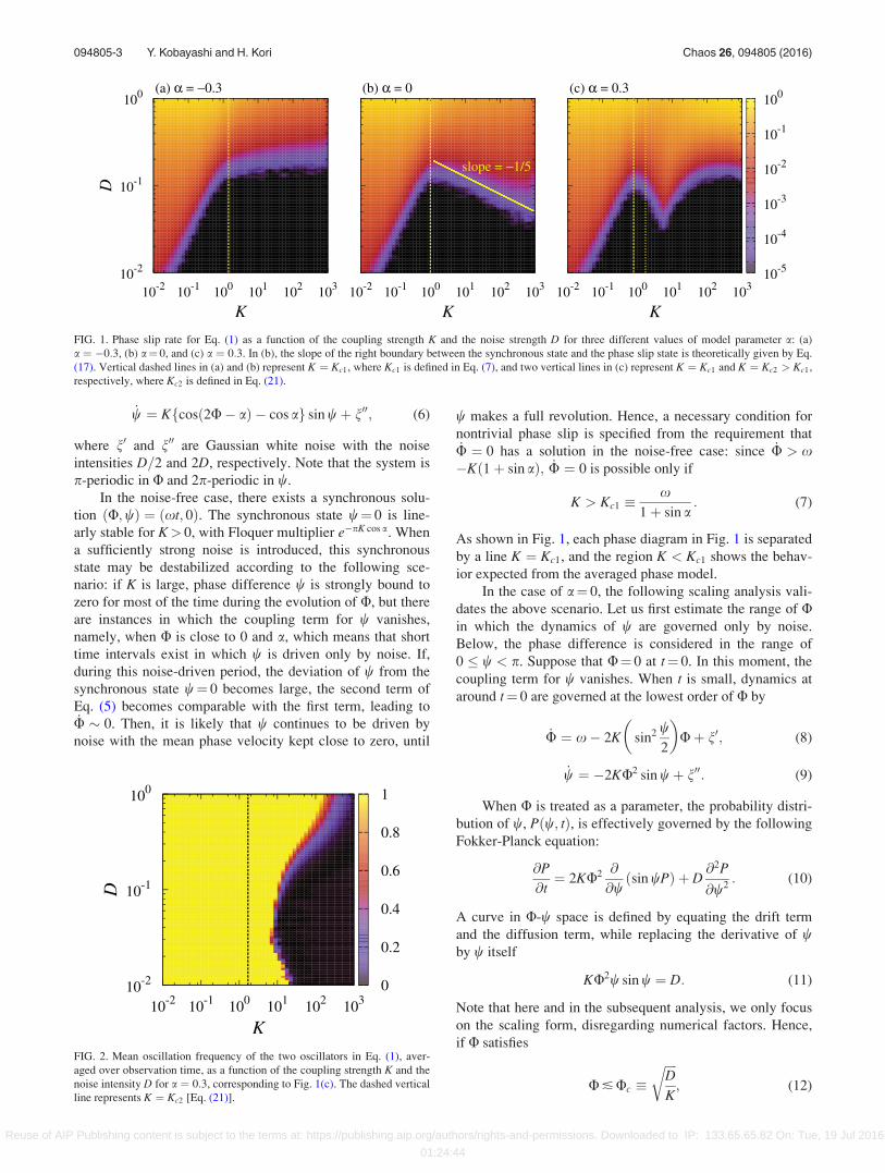
Figure 1 shows the slip rate as a function of the coupling

strength K and the noise intensity D for three different a val-

ues. The phase slip predicted by the averaged model3,15 is

observed for all cases where D>K. In addition to this trivial

type of phase slip, reentrant transitions are also observed for

a range of D when a � 0. In particular, for a¼ 0, the second

transition line follows a power law with an exponent close to

�0.2. For a ¼ 0:3, the reentrant transition line has a steeper

slope. Also, for large K, the phase slip region is invaded

by the region of oscillation death. Figure 2 plots the mean

oscillation frequency of the two oscillators, averaged over

observation time tmax, with the average frequency for each

oscillator given by hxii � 1tmax

Ð tmax

0_/idt. The black region

indicates that oscillation completely stops. No such oscilla-

tion death is observed for a � 0. For a ¼ �0:3, the reentrant

region disappears, although nontrivial phase slip is observed

for D<K. We have numerically confirmed that there are no

reentrant regions observed for at least a < �0:1 and that the

region of nontrivial phase slip diminishes as a decreases.

The overall tendency of phase slip for different a is

similar to our previous result for unilateral coupling

[Eq. (4)] in that the model shows reentrant transitions and

the nontrivial phase slip region expands as a increases,

although there are differences too. In the case of unilateral

coupling, no oscillation death is observed, which is obvious

because of the existence of the pacemaker. Further, the

power law exponent, which also appears in the case of uni-

lateral coupling when a¼ 0, is theoretically estimated and

numerically confirmed15 to be � 13, which is far from the

value of �0.2 observed in Fig. 1(b). The difference between

the exponents indicates that the mechanism of phase slip

differs from the case of unilateral interaction, which is

investigated below.

A. Nontrivial phase slip

Let us investigate how the phase slip occurs for strong

coupling. To do this, we rewrite model (1) in terms of mean

phase U � /1þ/2

2and phase difference w � /1 � /2

_U ¼ x� K sin2 w2

sin 2U� að Þ þ sin a� �

þ n0; (5)

094805-2 Y. Kobayashi and H. Kori Chaos 26, 094805 (2016)

Reuse of AIP Publishing content is subject to the terms at: https://publishing.aip.org/authors/rights-and-permissions. Downloaded to IP: 133.65.65.82 On: Tue, 19 Jul 2016

01:24:44

_w ¼ Kfcosð2U� aÞ � cos ag sin wþ n00; (6)

where n0 and n00 are Gaussian white noise with the noise

intensities D=2 and 2D, respectively. Note that the system is

p-periodic in U and 2p-periodic in w.

In the noise-free case, there exists a synchronous solu-

tion ðU;wÞ ¼ ðxt; 0Þ. The synchronous state w¼ 0 is line-

arly stable for K> 0, with Floquer multiplier e�pK cos a. When

a sufficiently strong noise is introduced, this synchronous

state may be destabilized according to the following sce-

nario: if K is large, phase difference w is strongly bound to

zero for most of the time during the evolution of U, but there

are instances in which the coupling term for w vanishes,

namely, when U is close to 0 and a, which means that short

time intervals exist in which w is driven only by noise. If,

during this noise-driven period, the deviation of w from the

synchronous state w¼ 0 becomes large, the second term of

Eq. (5) becomes comparable with the first term, leading to_U � 0. Then, it is likely that w continues to be driven by

noise with the mean phase velocity kept close to zero, until

w makes a full revolution. Hence, a necessary condition for

nontrivial phase slip is specified from the requirement that_U ¼ 0 has a solution in the noise-free case: since _U > x�Kð1þ sin aÞ; _U ¼ 0 is possible only if

K > Kc1 �x

1þ sin a: (7)

As shown in Fig. 1, each phase diagram in Fig. 1 is separated

by a line K ¼ Kc1, and the region K < Kc1 shows the behav-

ior expected from the averaged phase model.

In the case of a¼ 0, the following scaling analysis vali-

dates the above scenario. Let us first estimate the range of Uin which the dynamics of w are governed only by noise.

Below, the phase difference is considered in the range of

0 � w < p. Suppose that U¼ 0 at t¼ 0. In this moment, the

coupling term for w vanishes. When t is small, dynamics at

around t¼ 0 are governed at the lowest order of U by

_U ¼ x� 2K sin2 w2

� �Uþ n0; (8)

_w ¼ �2KU2 sin wþ n00: (9)

When U is treated as a parameter, the probability distri-

bution of w, Pðw; tÞ, is effectively governed by the following

Fokker-Planck equation:

@P

@t¼ 2KU2 @

@wsin wPð Þ þ D

@2P

@w2: (10)

A curve in U-w space is defined by equating the drift term

and the diffusion term, while replacing the derivative of wby w itself

KU2w sin w ¼ D: (11)

Note that here and in the subsequent analysis, we only focus

on the scaling form, disregarding numerical factors. Hence,

if U satisfies

U � Uc �ffiffiffiffiD

K

r; (12)

FIG. 1. Phase slip rate for Eq. (1) as a function of the coupling strength K and the noise strength D for three different values of model parameter a: (a)

a ¼ �0:3, (b) a¼ 0, and (c) a ¼ 0:3. In (b), the slope of the right boundary between the synchronous state and the phase slip state is theoretically given by Eq.

(17). Vertical dashed lines in (a) and (b) represent K ¼ Kc1, where Kc1 is defined in Eq. (7), and two vertical lines in (c) represent K ¼ Kc1 and K ¼ Kc2 > Kc1,

respectively, where Kc2 is defined in Eq. (21).

FIG. 2. Mean oscillation frequency of the two oscillators in Eq. (1), aver-

aged over observation time, as a function of the coupling strength K and the

noise intensity D for a ¼ 0:3, corresponding to Fig. 1(c). The dashed vertical

line represents K ¼ Kc2 [Eq. (21)].

094805-3 Y. Kobayashi and H. Kori Chaos 26, 094805 (2016)

Reuse of AIP Publishing content is subject to the terms at: https://publishing.aip.org/authors/rights-and-permissions. Downloaded to IP: 133.65.65.82 On: Tue, 19 Jul 2016

01:24:44

then the effect of the drift term is dominated by the diffusion

term for the whole range of w. Conversely, if U > Uc, the

drift term becomes effective. If U evolves as U ¼ xt, we can

determine the critical time tc at which U reaches Uc

tc ¼1

x

ffiffiffiffiD

K

r: (13)

Now consider a trajectory starting from ðU;wÞ ¼ ð0; 0Þat t¼ 0. The typical diffusion length of w at t¼ tc is given by

w1 ¼ffiffiffiffiffiffiffiDtc

p¼ x�

12D

34K�

14: (14)

Moreover, _U ¼ 0 with D¼ 0 determines another curve

in U-w space

KU sin2 w2¼ x: (15)

For large K, this curve and the other curve given by Eq. (11)

cross each other, where w ¼ w2 at the intersection is shown

to be small. Indeed, by expanding Eqs. (11) and (15) in terms

of w, w2 is obtained as

w2 ¼ x12D�

12K�

12; (16)

which diminishes as K increases. In order that the trajectory

reaches the curve (15) before it gets affected by the drift

term, the diffusion length w1 must be greater than w2. The

critical transition line is given by w1 ¼ w2, which yields the

scaling form

D ¼ x45K�

15; (17)

which implies that, for a fixed D value, the phase slip

becomes more and more frequent as K increases. This scal-

ing relation is in good agreement with the numerically

obtained reentrant transition line in Fig. 1(b).

As mentioned above, the unilateral coupling case shows

a different scaling relation D ¼ x43K�

13, which indicates that

the reentrant region is narrower in the present case than in

the unilateral case.

B. Oscillation death

In the noise-free case, in addition to the synchronous so-

lution ðU;wÞ ¼ ðxt; 0Þ, the system may have steady state

solutions, which correspond to oscillation death, depending

on the parameters K and a. Here, without loss of generality,

we restrict the range of U and w to 0 � U < p and

0 � w < 2p, respectively. Steady states are given by _U ¼ 0

and _w ¼ 0 in Eqs. (5) and (6) with D¼ 0, which are satisfied

by ðU;wÞ ¼ ðU; pÞ and ðU;wÞ ¼ ða;wÞ, where U and w

are determined by

x� Kfsinð2U � aÞ þ sin ag ¼ 0; (18)

and

x� 2K sin a sin2 w

2¼ 0; (19)

respectively.

The solution U to Eq. (18) exists only when inequality

(7) is satisfied. At K ¼ Kc1, two solutions U ¼ Ua and U

¼ Ub appear as a result of saddle-node bifurcation, where

Ua ¼a2þ h

2; Ub ¼

a2þ p� h

2; (20)

and h ¼ arcsin xK � sin aÞ�

. Linear stability analysis shows

that at the onset of bifurcation, U ¼ Ua and U ¼ Ub corre-

spond to a saddle and an unstable focus, respectively. The

unstable eigenvalue for the saddle is given by k ¼ Kðcos a

�ffiffiffiffiffiffiffiffiffiffiffiffiffiffiffiffiffiffiffiffiffiffiffiffiffiffiffiffiffiffiffi1� ðxK � sin aÞ2

qÞ. Hence, at K ¼ Kc2 > Kc1, secondary

bifurcation occurs, where Kc2 is determined by k¼ 0. It is

easy to see that if a � 0, then there is no such Kc2 that satis-

fies k¼ 0. If a > 0, this yields

Kc2 ¼x

2 sin a: (21)

For K > Kc2 and a > 0, Eq. (19) also has two solutions

w ¼ b and w ¼ 2p� b, where b ¼ 2arcsinffiffiffiffiffiffiffiffiffiffiffi

x2K sin a

p. Linear

stability analysis shows that these two branches are saddles,

which originate from ðU;wÞ ¼ ðUa; pÞ at K ¼ Kc2 by pitch-

fork bifurcation. Note that h ¼ a and b ¼ p at K ¼ Kc2, and

therefore ðUa; pÞ ¼ ða;wÞ at this point. At K > Kc2, point

ðUa; pÞ becomes a stable focus, which corresponds to the

death state.

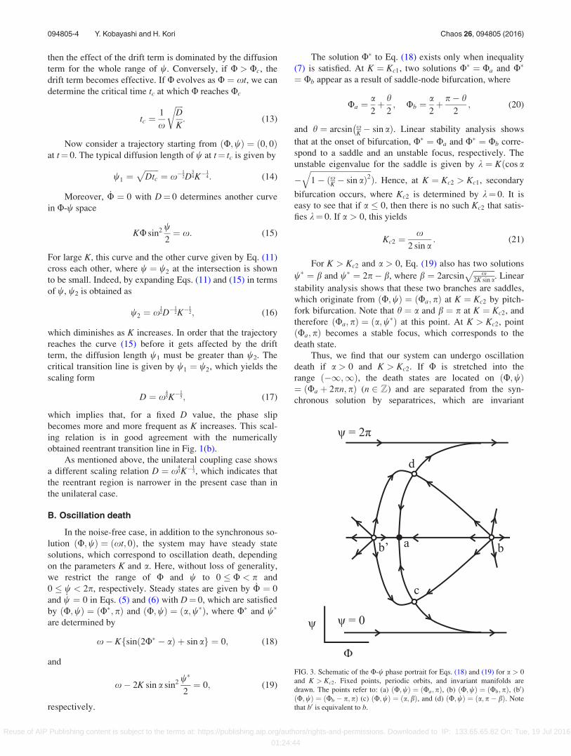
Thus, we find that our system can undergo oscillation

death if a > 0 and K > Kc2. If U is stretched into the

range ð�1;1Þ, the death states are located on ðU;wÞ¼ ðUa þ 2pn; pÞ (n 2 Z) and are separated from the syn-

chronous solution by separatrices, which are invariant

FIG. 3. Schematic of the U-w phase portrait for Eqs. (18) and (19) for a > 0

and K > Kc2. Fixed points, periodic orbits, and invariant manifolds are

drawn. The points refer to: (a) ðU;wÞ ¼ ðUa;pÞ, (b) ðU;wÞ ¼ ðUb;pÞ, (b0)ðU;wÞ ¼ ðUb � p; pÞ (c) ðU;wÞ ¼ ða; bÞ, and (d) ðU;wÞ ¼ ða; p� bÞ. Note

that b0 is equivalent to b.

094805-4 Y. Kobayashi and H. Kori Chaos 26, 094805 (2016)

Reuse of AIP Publishing content is subject to the terms at: https://publishing.aip.org/authors/rights-and-permissions. Downloaded to IP: 133.65.65.82 On: Tue, 19 Jul 2016

01:24:44

manifolds connecting the unstable foci ðU;wÞ ¼ ðUb þ2pðn� 1Þ; pÞ and ðUb þ 2pn; pÞ and the saddles ðU;wÞ ¼ðaþ 2pn; bÞ and ðaþ 2pn; 2p� bÞ (see Fig. 3). These sepa-

ratrices can be overcome when a sufficiently strong noise is

applied to the system.

It is possible that the conditions for nontrivial phase slip

and oscillation death are both satisfied. Since nontrivial

phase slip occurs along _U ¼ 0, the trajectory is likely to be

trapped during a slip event by the death state ðUa; pÞ, which

is located on the line _U ¼ 0. Then, the probability of trap-

ping depends on the noise intensity, as indicated in Fig. 2:

for a fixed K > Kc2, strong noise aids escape from the death

state; conversely, weak noise is not sufficient to escape from

the synchronous state. Thus, the boundary of the death state

moves rightward for large and small D values.

III. NETWORK-CONNECTED SYSTEM

Now, we consider N coupled phase oscillators with

frequency x under noise. The i-th oscillator obeys

_/i ¼ xþ KZð/iÞXN

j¼1

Aijfhð/jÞ � hð/iÞg þ ni; (22)

where Z and h are given by Eq. (2), and ni is the same as

before. Their connections are determined by adjacency ma-

trix A. We investigate synchronizability of the following net-

works: scale-free networks generated by the Barab�asi-Albert

(BA) algorithm19 with the minimum degree m0 ¼ 1 with net-

work size N¼ 100 (average degree hdi ¼ 2:0) or N¼ 10 000

(hdi ¼ 2:0), and m0 ¼ 3 with N¼ 10 000 (hdi ¼ 6:0); an

all-to-all connection with N¼ 100 (hdi ¼ 99); and an Erd}os-

R�enyi random network with N¼ 400 (hdi ¼ 5:8). Since we

are interested in destabilization of the synchronous state, we

start with a synchronous initial condition with weak random

perturbations in the range ð�0:01p; 0:01pÞ given to individ-

ual oscillators.

For a given network, a phase slip event of the ith node is

counted when a full revolution of /i in the positive or nega-

tive direction is made with respect to the mean phase of the

rest of the oscillators: the phase difference for i is defined

as wj � /j � 1N�1

Pi 6¼j/i ¼ N

N�1/j � UN�

, where UN � 1NPN

j¼1 /j is the mean phase of all oscillators. The phase slip

rate of oscillator i is then the total number of phase slip

events divided by the observation time tmax, which in the fol-

lowing simulations is tmax ¼ 104.

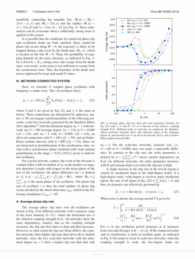
A. Average phase slip rate

The average phase slip rates over all oscillators are

shown in Fig. 4 for different networks with a nonzero value

of the noise intensity D¼ 0.1, where the horizontal axis is

the effective coupling strength Khdi. All networks show the

same dependency, namely, that as the coupling strength

increases, the slip rate first starts to drop and then increases.

However, to what extent the slip rate drops differs: the scale-

free networks show higher slip rates than all-to-all or random

networks. Also, the two scale-free networks with the mini-

mum degree m0 ¼ 1 show a higher slip rate than that with

m0 ¼ 3. For the scale-free networks, network size, i.e.,

N¼ 100 or N¼ 10 000, does not make a noticeable differ-

ence. In contrast to the slip rate, the order parameter r

defined by r ¼ j 1N

PNi¼1 ei/i j shows similar dependence on

Khdi for different networks: the order parameter increases

with K and remains high even when the slip rate is high.

A slight increase in the slip rate in the low-K region is

caused by incoherent input to the high-degree nodes: if a

high-degree node i with degree di receives many incoherent

inputs, the sum of all inputs in Eq. (22) isP

ihð/iÞ � 0, and

thus, its dynamics are effectively governed by

_/i ¼ xþ Kdi sinð/i � aÞ cos /i þ ni: (23)

When noise is absent, the average period T is given by

T ¼ð2p

0

d/xþ Kdi sin /� að Þcos /

¼ 2px

1� Kdi

xsin a� K2d2

i

4x2cos2a

�12

: (24)

For a¼ 0, the oscillation period increases as K increases

from zero and diverges at K ¼ 2x=di. If the connected nodes

start to synchronize, it starts to oscillate again. As indicated

in Fig. 4, this tends to occur in scale-free networks: when the

coupling strength is weak, the low-degree nodes are

FIG. 4. Average phase slip rate (top) and order parameter (bottom) for

Eq. (22) with a¼ 0 and D¼ 0.1 as a function of the effective coupling

strength Khdi. Different kinds of networks are employed: the Barab�asi-

Albert scale-free networks (BA) with different values of the minimum

degree m0 and network size N; an all-to-all network (ALL); and an Erd}os-

R�enyi random network (ER).

094805-5 Y. Kobayashi and H. Kori Chaos 26, 094805 (2016)

Reuse of AIP Publishing content is subject to the terms at: https://publishing.aip.org/authors/rights-and-permissions. Downloaded to IP: 133.65.65.82 On: Tue, 19 Jul 2016

01:24:44

incoherent, and the high-degree nodes receive a lot of such

incoherent signals.

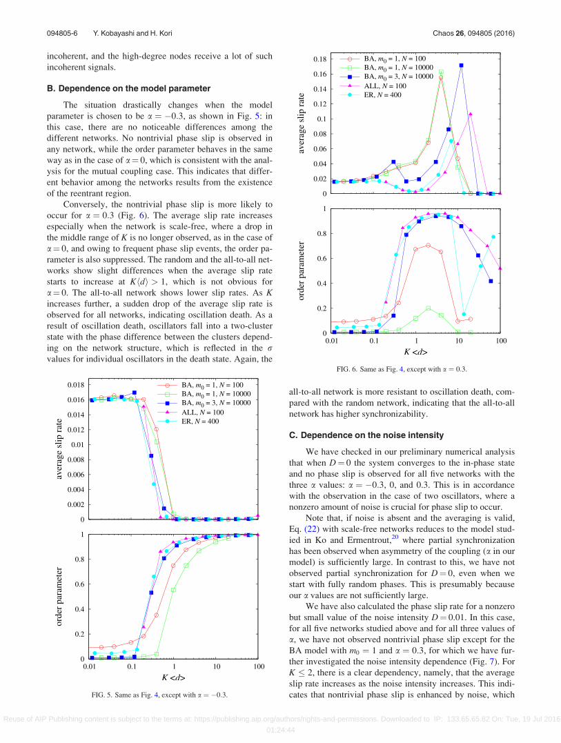
B. Dependence on the model parameter

The situation drastically changes when the model

parameter is chosen to be a ¼ �0:3, as shown in Fig. 5: in

this case, there are no noticeable differences among the

different networks. No nontrivial phase slip is observed in

any network, while the order parameter behaves in the same

way as in the case of a¼ 0, which is consistent with the anal-

ysis for the mutual coupling case. This indicates that differ-

ent behavior among the networks results from the existence

of the reentrant region.

Conversely, the nontrivial phase slip is more likely to

occur for a ¼ 0:3 (Fig. 6). The average slip rate increases

especially when the network is scale-free, where a drop in

the middle range of K is no longer observed, as in the case of

a¼ 0, and owing to frequent phase slip events, the order pa-

rameter is also suppressed. The random and the all-to-all net-

works show slight differences when the average slip rate

starts to increase at Khdi > 1, which is not obvious for

a¼ 0. The all-to-all network shows lower slip rates. As Kincreases further, a sudden drop of the average slip rate is

observed for all networks, indicating oscillation death. As a

result of oscillation death, oscillators fall into a two-cluster

state with the phase difference between the clusters depend-

ing on the network structure, which is reflected in the rvalues for individual oscillators in the death state. Again, the

all-to-all network is more resistant to oscillation death, com-

pared with the random network, indicating that the all-to-all

network has higher synchronizability.

C. Dependence on the noise intensity

We have checked in our preliminary numerical analysis

that when D¼ 0 the system converges to the in-phase state

and no phase slip is observed for all five networks with the

three a values: a ¼ �0:3, 0, and 0.3. This is in accordance

with the observation in the case of two oscillators, where a

nonzero amount of noise is crucial for phase slip to occur.

Note that, if noise is absent and the averaging is valid,

Eq. (22) with scale-free networks reduces to the model stud-

ied in Ko and Ermentrout,20 where partial synchronization

has been observed when asymmetry of the coupling (a in our

model) is sufficiently large. In contrast to this, we have not

observed partial synchronization for D¼ 0, even when we

start with fully random phases. This is presumably because

our a values are not sufficiently large.

We have also calculated the phase slip rate for a nonzero

but small value of the noise intensity D¼ 0.01. In this case,

for all five networks studied above and for all three values of

a, we have not observed nontrivial phase slip except for the

BA model with m0 ¼ 1 and a ¼ 0:3, for which we have fur-

ther investigated the noise intensity dependence (Fig. 7). For

K � 2, there is a clear dependency, namely, that the average

slip rate increases as the noise intensity increases. This indi-

cates that nontrivial phase slip is enhanced by noise, whichFIG. 5. Same as Fig. 4, except with a ¼ �0:3.

FIG. 6. Same as Fig. 4, except with a ¼ 0:3.

094805-6 Y. Kobayashi and H. Kori Chaos 26, 094805 (2016)

Reuse of AIP Publishing content is subject to the terms at: https://publishing.aip.org/authors/rights-and-permissions. Downloaded to IP: 133.65.65.82 On: Tue, 19 Jul 2016

01:24:44

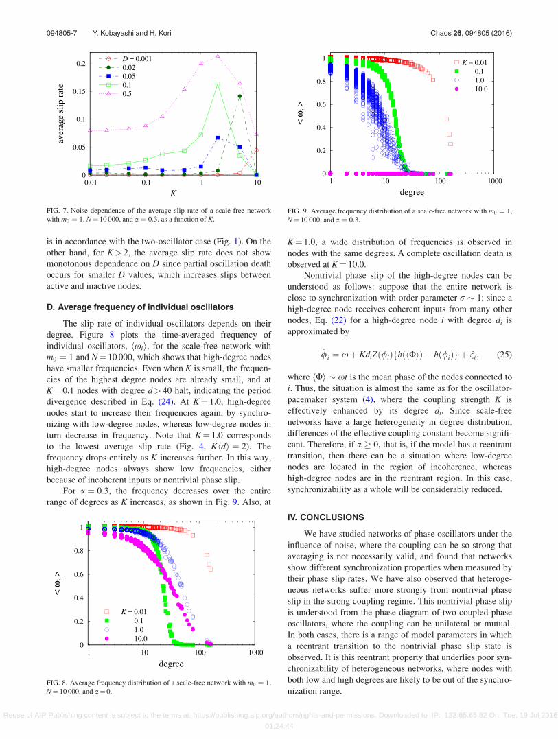
is in accordance with the two-oscillator case (Fig. 1). On the

other hand, for K> 2, the average slip rate does not show

monotonous dependence on D since partial oscillation death

occurs for smaller D values, which increases slips between

active and inactive nodes.

D. Average frequency of individual oscillators

The slip rate of individual oscillators depends on their

degree. Figure 8 plots the time-averaged frequency of

individual oscillators, hxii, for the scale-free network with

m0 ¼ 1 and N¼ 10 000, which shows that high-degree nodes

have smaller frequencies. Even when K is small, the frequen-

cies of the highest degree nodes are already small, and at

K¼ 0.1 nodes with degree d> 40 halt, indicating the period

divergence described in Eq. (24). At K¼ 1.0, high-degree

nodes start to increase their frequencies again, by synchro-

nizing with low-degree nodes, whereas low-degree nodes in

turn decrease in frequency. Note that K¼ 1.0 corresponds

to the lowest average slip rate (Fig. 4, Khdi ¼ 2). The

frequency drops entirely as K increases further. In this way,

high-degree nodes always show low frequencies, either

because of incoherent inputs or nontrivial phase slip.

For a ¼ 0:3, the frequency decreases over the entire

range of degrees as K increases, as shown in Fig. 9. Also, at

K¼ 1.0, a wide distribution of frequencies is observed in

nodes with the same degrees. A complete oscillation death is

observed at K¼ 10.0.

Nontrivial phase slip of the high-degree nodes can be

understood as follows: suppose that the entire network is

close to synchronization with order parameter r � 1; since a

high-degree node receives coherent inputs from many other

nodes, Eq. (22) for a high-degree node i with degree di is

approximated by

_/i ¼ xþ KdiZð/iÞfhðhUiÞ � hð/iÞg þ ni; (25)

where hUi � xt is the mean phase of the nodes connected to

i. Thus, the situation is almost the same as for the oscillator-

pacemaker system (4), where the coupling strength K is

effectively enhanced by its degree di. Since scale-free

networks have a large heterogeneity in degree distribution,

differences of the effective coupling constant become signifi-

cant. Therefore, if a � 0, that is, if the model has a reentrant

transition, then there can be a situation where low-degree

nodes are located in the region of incoherence, whereas

high-degree nodes are in the reentrant region. In this case,

synchronizability as a whole will be considerably reduced.

IV. CONCLUSIONS

We have studied networks of phase oscillators under the

influence of noise, where the coupling can be so strong that

averaging is not necessarily valid, and found that networks

show different synchronization properties when measured by

their phase slip rates. We have also observed that heteroge-

neous networks suffer more strongly from nontrivial phase

slip in the strong coupling regime. This nontrivial phase slip

is understood from the phase diagram of two coupled phase

oscillators, where the coupling can be unilateral or mutual.

In both cases, there is a range of model parameters in which

a reentrant transition to the nontrivial phase slip state is

observed. It is this reentrant property that underlies poor syn-

chronizability of heterogeneous networks, where nodes with

both low and high degrees are likely to be out of the synchro-

nization range.

FIG. 7. Noise dependence of the average slip rate of a scale-free network

with m0 ¼ 1, N¼ 10 000, and a ¼ 0:3, as a function of K.

FIG. 8. Average frequency distribution of a scale-free network with m0 ¼ 1,

N¼ 10 000, and a¼ 0.

FIG. 9. Average frequency distribution of a scale-free network with m0 ¼ 1,

N¼ 10 000, and a ¼ 0:3.

094805-7 Y. Kobayashi and H. Kori Chaos 26, 094805 (2016)

Reuse of AIP Publishing content is subject to the terms at: https://publishing.aip.org/authors/rights-and-permissions. Downloaded to IP: 133.65.65.82 On: Tue, 19 Jul 2016

01:24:44

ACKNOWLEDGMENTS

H.K. acknowledges financial support from CREST, JST.

1A. T. Winfree, The Geometry of Biological Time, 2nd ed. (Springer-

Verlag, New York, 2001).2Y. Kuramoto, Chemical Oscillations, Waves, and Turbulence (Springer-

Verlag, New York, 1984).3A. Pikovsky, M. Rosenblum, and J. Kurths, Synchronization: A UniversalConcept in Nonlinear Sciences (Cambridge University Press, New York,

2001).4L. Glass, “Synchronization and rhythmic processes in physiology,” Nature

410, 277 (2001).5I. Z. Kiss, C. G. Rusin, H. Kori, and J. L. Hudson, “Engineering complex

dynamical structures: Sequential patterns and desynchronization,” Science

316, 1886 (2007).6L. H. van der Tweel, F. L. Meijler, and F. J. L. van Capelle,

“Synchronization of the heart,” J. Appl. Physiol. 34, 283 (1973), available

at http://jap.physiology.org/content/34/2/283.7S. M. Reppert and D. R. Weaver, “Coordination of circadian timing in

mammals,” Nature 418, 935 (2002).8S. Yamaguchi, H. Isejima, T. Matsuo, R. Okura, K. Yagita, M. Kobayashi,

and H. Okamura, “Synchronization of cellular clocks in the suprachias-

matic nucleus,” Science 302, 1408 (2003).9A. E. Motter, S. A. Myers, M. Anghel, and T. Nishikawa, “Spontaneous

synchrony in power-grid networks,” Nat. Phys. 9, 191 (2013).

10F. D€orfler, M. Chertkov, and F. Bullo, “Synchronization in complex oscil-

lator networks and smart grids,” Proc. Natl. Acad. Sci. U. S. A. 110, 2005

(2013).11M. Rohden, A. Sorge, M. Timme, and D. Witthaut, “Self-organized syn-

chronization in decentralized power grids,” Phys. Rev. Lett. 109, 064101

(2012).12H. Fujisaka and T. Yamada, “Stability theory of synchronized motion in

coupled-oscillator systems,” Prog. Theor. Phys. 69, 32 (1983).13J. F. Heagy, T. L. Carroll, and L. M. Pecora, “Synchronous chaos in

coupled oscillator systems,” Phys. Rev. E 50, 1874 (1994).14T. Nishikawa, A. E. Motter, Y. C. Lai, and F. C. Hoppensteadt,

“Heterogeneity in oscillator networks: Are smaller world easier to syn-

chronize?,” Phys. Rev. Lett. 91, 014101 (2003).15Y. Kobayashi and H. Kori, “Reentrant transition in coupled noisy oscil-

lators,” Phys. Rev. E 91, 012901 (2015).16A. T. Winfree, “Biological rhythms and the behavior of populations of

coupled oscillators,” J. Theor. Biol. 16, 15 (1967).17F. C. Hoppensteadt and E. M. Izhikevich, Weakly Connected Neural

Networks (Springer-Verlag, New York, 1997).18H. Sakaguchi and Y. Kuramoto, “A soluble active rotater model showing

phase transitions via mutual entrainment,” Prog. Theor. Phys. 76, 576

(1986).19R. Albert and A.-L. Barab�asi, “Statistical mechanics of complex

networks,” Rev. Mod. Phys. 74, 47 (2002).20T.-W. Ko and G. B. Ermentrout, “Partially locked states in coupled oscil-

lators due to inhomogeneous coupling,” Phys. Rev. E 78, 016203 (2008).

094805-8 Y. Kobayashi and H. Kori Chaos 26, 094805 (2016)

Reuse of AIP Publishing content is subject to the terms at: https://publishing.aip.org/authors/rights-and-permissions. Downloaded to IP: 133.65.65.82 On: Tue, 19 Jul 2016

01:24:44