synchronization of operating systems in … of operating systems in heterogeneous testing...

Distributed Systems

Synchronization of OperatingSystems in Heterogeneous

Testing Environments

RWTH Aachen UniversityLuFG Informatik 4 Distributed Systems

Diploma Thesis

Florian Schmidt

Advisors:

Dipl-Inf. Elias WeingartnerProf. Dr.-Ing. Klaus Wehrle

Registration date: 12 December 2007Submission Date: 12 June 2008

I hereby affirm that I composed this work independently and used no other than thespecified sources and tools and that I marked all quotes as such.

Ich erklare hiermit, dass ich die vorliegende Arbeit selbstandig verfasst und keineanderen als die angegebenen Quellen und Hilfsmittel verwendet habe.

Aachen, den 12. Juni 2008

Kurzfassung

Die Entwicklung und Analyse von Software durchlauft im Normalfall mehrere Phasen.Am Anfang steht ein Konzept, das im Fall von Netzwerkprotokolldesign in einemNetzwerksimulator getestet werden kann. Schließlich erfolgt die Entwicklung einesPrototyps zur Analyse einer konkreten Implementierung. Simulation und Proto-typen haben beide ihre spezifischen Vor- und Nachteile. Netzwerkemulation erlaubtdie Verknupfung beider Ansatze, allerdings muss fur eine realistische Analyse im Hin-blick auf das Zeitverhalten die Simulation in Echtzeit ablaufen konnen. Dies ist inkomplexeren Simulationsszenarien nicht gewahrleistet. Diese Diplomarbeit entwirftund setzt eine Testumgebung um, die durch Kapselung eines x86-Systems in Xeneine Synchronisation der Implementierung mit beliebig komplexen und langsamenSimulationen erlaubt und gleichzeitig eine Analyse des Zeitverhaltens ermoglicht.

Abstract

Software design generally employs different techniques in different phases for anal-ysis. In the beginning, a new network protocol may be conceptualized and testedin a network simulator. Later on, a prototype of the actual implementation is thor-oughly analyzed. Both approaches have their specific up- and downsides. Networkemulation allows to combine both to gather additional data and facilitate easierprototype testbed layouts. For meaningful analysis however, especially in regard totiming behavior, the simulation has to be real-time capable. This is often not thecase for complex simulated scenarios. This diploma thesis designs and implements asynchronization that allows to run any x86 operating system with arbitrarily com-plex simulations. By encapsulating the OS in the Xen hypervisor, it relieves thesimulation from the real-time capability constraint while still maintaining realistictiming behavior.

Acknowledgments

A work such as this is never the result of one person working all alone. I want to usethis opportunity to thank all the people who made it possible to write this thesis,and helped in improving it:

Prof. Dr. Wehrle, for giving me the opportunity to write this thesis at the distributedsystems group, and for being my supervisor.

Prof. Dr. Kowaleswki, for kindly agreeing to be my second supervisor for this thesis.

My advisor, Elias Weingartner, for sparking in me the interest in the topics of syn-chronization and virtualization, for always taking time for discussions of problemsand solutions, and for being a great motivator.

Ismet Aktas, for always being supportive, and for having strong belief in my skills,sometimes more than myself—and he was right.

All members of the distributed systems group, especially Stefan Gotz and Olaf Land-siedel, for many interesting and fruitful discussions, and for contributing to the ex-cellent work atmosphere.

My brother Gereon, Corinna Habets, and David Piegdon, for helping me proofreadthis text.

Finally, my parents, for always supporting me during the not always easy time ofmy studies.

Contents

1 Introduction 1

2 Background 5

2.1 Network Simulation . . . . . . . . . . . . . . . . . . . . . . . . . . . . 5

2.1.1 The OMNeT++ Discrete Event Simulator . . . . . . . . . . . 6

2.1.2 The INET Framework . . . . . . . . . . . . . . . . . . . . . . 7

2.2 Prototyping . . . . . . . . . . . . . . . . . . . . . . . . . . . . . . . . 8

2.3 Emulation . . . . . . . . . . . . . . . . . . . . . . . . . . . . . . . . . 9

2.4 Synchronization . . . . . . . . . . . . . . . . . . . . . . . . . . . . . . 10

2.5 Virtualization . . . . . . . . . . . . . . . . . . . . . . . . . . . . . . . 14

2.5.1 The Xen Hypervisor . . . . . . . . . . . . . . . . . . . . . . . 16

2.5.2 Paravirtualization . . . . . . . . . . . . . . . . . . . . . . . . . 18

2.5.3 Hardware Virtualization . . . . . . . . . . . . . . . . . . . . . 19

2.5.4 Comparison of Virtual Machine Monitors . . . . . . . . . . . . 20

2.6 The Xen sEDF Scheduler . . . . . . . . . . . . . . . . . . . . . . . . . 20

2.7 Timekeeping . . . . . . . . . . . . . . . . . . . . . . . . . . . . . . . . 24

3 Implementation 27

3.1 The Synchronization Server . . . . . . . . . . . . . . . . . . . . . . . 28

3.2 The Synchronization Client . . . . . . . . . . . . . . . . . . . . . . . 29

3.2.1 The Xen Synchronization Client . . . . . . . . . . . . . . . . . 29

3.2.2 The OMNeT++ Synchronization Client . . . . . . . . . . . . 31

3.3 The Emulator . . . . . . . . . . . . . . . . . . . . . . . . . . . . . . . 32

3.4 Modifications to Xen . . . . . . . . . . . . . . . . . . . . . . . . . . . 33

3.4.1 Modifications to the sEDF Scheduler . . . . . . . . . . . . . . 34

3.4.1.1 Misattribution of Runtime . . . . . . . . . . . . . . . 35

3.4.1.2 The sEDF Interface . . . . . . . . . . . . . . . . . . 37

3.4.2 Time Warping: Modifications to the Timekeeping Subsystem . 38

3.4.2.1 Paravirtualization . . . . . . . . . . . . . . . . . . . 39

3.4.2.2 Hardware Virtualization . . . . . . . . . . . . . . . . 40

3.4.3 Miscellaneous Changes to Xen and the dom0 Kernel . . . . . . 42

4 Evaluation 45

4.1 Timing Accuracy . . . . . . . . . . . . . . . . . . . . . . . . . . . . . 45

4.2 Overhead . . . . . . . . . . . . . . . . . . . . . . . . . . . . . . . . . 48

4.3 CPU Performance . . . . . . . . . . . . . . . . . . . . . . . . . . . . . 50

4.4 Network Throughput Performance . . . . . . . . . . . . . . . . . . . . 51

4.5 Summary . . . . . . . . . . . . . . . . . . . . . . . . . . . . . . . . . 55

5 Related Work 57

5.1 Discrete Event Simulation . . . . . . . . . . . . . . . . . . . . . . . . 57

5.2 Opaque Network Simulation . . . . . . . . . . . . . . . . . . . . . . . 59

5.3 Emulation . . . . . . . . . . . . . . . . . . . . . . . . . . . . . . . . . 61

5.4 Encapsulation of Real Systems . . . . . . . . . . . . . . . . . . . . . . 63

5.5 Extensions to Xen . . . . . . . . . . . . . . . . . . . . . . . . . . . . 64

6 Future Work 67

6.1 Synchronizing Virtualized SMP Systems . . . . . . . . . . . . . . . . 67

6.1.1 Case 1: Number of VCPUs Lower Than or Equal To Numberof PCPUs . . . . . . . . . . . . . . . . . . . . . . . . . . . . . 68

6.1.2 Case 2: Number of VCPUs Greater Than Number of PCPUs . 69

6.2 Network Throughput Performance . . . . . . . . . . . . . . . . . . . . 70

6.3 Introspection and Probing . . . . . . . . . . . . . . . . . . . . . . . . 71

7 Conclusion 73

Bibliography 77

A Synchronization System Setup 83

A.1 Configuration Options . . . . . . . . . . . . . . . . . . . . . . . . . . 83

A.1.1 Stand-Alone Synchronization Server . . . . . . . . . . . . . . . 83

A.1.2 Xen Synchronization Client . . . . . . . . . . . . . . . . . . . 84

A.1.3 OMNeT++ Synchronization Client–Scheduler . . . . . . . . . 84

A.1.4 Emulator–Tunnel: Xen Side . . . . . . . . . . . . . . . . . . . 85

A.1.5 Emulator–Tunnel: OMNeT++ Side . . . . . . . . . . . . . . . 85

A.2 Synchronized Network Emulation Setup . . . . . . . . . . . . . . . . 86

1Introduction

Whenever a new piece of software is developed, it has to be tested for proper func-tionality. Furthermore, if it contains a new concept, such as (in the field of networkcommunications, which this thesis concentrates on) a new networking protocol, ithas to be analyzed to make sure there are no conceptual errors. Two importantways of analysis are simulation and prototyping. In simulation, the concept in itsabstract form is implemented to use it in a simulation environment, and then testsare run. The main advantage is that it is generally comparably easy to do the stepfrom concept to a simulation model in contrast to a full prototype that runs on anend-user system, and it allows for a great deal of flexibility. Once the functionality ofthe concept has been implemented in the simulation, networks of arbitrary size andcomplexity can be constructed for stress-testing, and tests can be rerun to closelyanalyze special cases.

However, simulations abstract from many factors that the final product has to dealwith, such as side-effects from hardware or operating system. At some point, it istherefore necessary to create a prototype and analyze it in a natural testbed envi-ronment. Testbeds are limited in size to a couple hundred of prototypes however,and the latter already introduces a massive cost and effort. Hardware for all thenodes inside the testbed has to be procured, and every time some part of the proto-type implementation is changed, all the prototypes have to be updated. Practicalitytherefore dictates the maximum number of prototype nodes in the testbed. This isunfortunate because it would be very desirable to analyze the performance of theprototype in more complex network topologies.

Consequently, it is desirable to find a way to combine prototyping with simulation.One way to reach this goal is network emulation, in which a prototype is connectedto the simulation by means of an emulator, that can translate between real net-work packets from the prototype, and packet messages from the simulator, so thatcommunication between the two is possible. The problem is that this only worksas long as the simulation is able to run at real-time speed. When it does not, re-sults measured are not correct in respect to timing information any more, which can

2 1. Introduction

lead to incorrect behavior. For example, a simulation might take so long to route apacket to the receiver, and afterwards the ACK packet back to the prototype, thatthe prototype assumes it has been lost and retransmits it. In the worst case, thiscan lead to an ever-increasing load on the simulation, to the point where it becomeslive-locked (events are created faster than they can be processed, and the simulationstalls). Unfortunately, simulations tend to run slower and lose their real-time capa-bilities the more complex the simulation is. But this is exactly the most interestinguse case for network emulation, since small networks can be feasibly analyzed witha testbed of prototypes only.

The solution would be to synchronize simulation and prototype to each other, sothat the faster can wait for the slower to catch up again. In this case, this means tostop the prototype. This, however, is easier said than done for end-user computersystems, such as the x86, since they keep track of time. Even if the operating systemis modified to sleep for certain periods until the simulation has caught up again, anumber of hardware clocks and timers inside the system will make it immediatelynoticeable that time has passed. To come back to the prior example, a retransmissiontimer would still expire at the same time as before, regardless whether the systemhas been put to sleep or not, which means nothing has been won.

Obviously, it is a very tantalizing thought to solve the synchronization problem innetwork emulation, because it would allow to analyze how prototype implementa-tions behave in large network, without the immense cost of creating a testbed ofthe same size. This thesis proposes a solution for x86 based systems. It uses theXen Hypervisor [9] to disconnect an operating system from directly accessing thehardware, and modifies it so that two goals are reached:

1. The Operating System must be stoppable and startable at any point in time,and run for precisely the amount of time assigned.

2. The Operating System must not notice that, during the time it did not run,any time passed. In other words, although it will run only intermittently, itmust seem to it as if time passed continuously without any gaps.

Under these two constraints, a system can be stopped whenever the simulation fallsbehind, and restarted after the latter has caught up. Throughout this work, they willbe referenced as “requirement 1” and “requirement 2”. The prototype can thereforebe synchronized to the simulation. The presented Xen implementation can maskthe passing of time from an OS during descheduled times and accurately control theexecution down to time slices of 10µs, which is therefore the maximum amount oftime the clocks inside simulation and prototype can ever differ.

To complete synchronization set-up, the author developed or reused a few othercomponents to make the synchronization work as a whole:

1. A central synchronization server∗ that makes sure no prototype or simulationdeviates from the common time by more than a predefined amount.

∗Developed by Elias Weingartner

3

2. A synchronization client† that runs on the same machine as the hypervisor,and interfaces with Xen to control the execution of the synchronized operatingsystem.

3. An OMNeT++ scheduler that interfaces with the synchronizer.∗

4. An emulator that translates between network packets and simulator messages,for the OMNeT++ simulator.‡

Note that on the one hand, while the work described in this thesis uses OMNeT++[69] as simulator, the changes are generic enough to be easily applicable to mostother discrete event network simulators. On the other hand, while the concept ofusing virtualization to encapsulate a prototype can be applied to other virtualizers,or even full-system simulators such as Simics [50], or processor emulators such asQEMU [12], the work done for this thesis is too specific as to allow for fast portingto those.

The rest of this diploma thesis is structured as follows: Chapter 2 will give anoverview over and background information on different components that are impor-tant to the understanding of the work done. The actual implementation, with anexplanation of how Xen has been changed to reach the two goals for synchroniza-tion outlined above, how the synchronizer works, etc. is presented in Chapter 3.Chapter 4 will analyze results of tests that have been conducted. Chapter 5 willdiscuss previous work done in related fields, while potential future fields of work willbe proposed in Chapter 6. Finally, Chapter 7 will give a summary.

†Own work∗Developed by Elias Weingartner‡Own work, parts of which have been adapted from an earlier work by Joachim Riedl [59].

4 1. Introduction

2Background

In any field of work that involves creating large numbers of a developed invention,testing and analysis are important steps from the initial idea to the final product.No car in the world is built right away from the initial concept art. Especially inengineering, the testing can take several years and will pass through different phases.

While the testing standards might not be quite as high in the field of computerscience, testing and analysis still play a vital role in the development of new commu-nication systems, such as network applications or communication protocols. Testingwill also typically pass through different phases. Early on, and for a long time duringthe development, simulation is a prime choice; later on, prototype implementationswill give additional insight into potential problems.

2.1 Network Simulation

The most widely used type of network simulation is discrete event simulation (DES).In this type of simulation, every action by any node that changes the simulation’soverall state is represented as an event. Every event, in turn, is assigned a certainpoint in time at which it will happen. The fact that an event is assigned a time inthe future at its creation time means that the simulation can maintain an orderedevent list at all times. This allows the simulation to advance directly to the nextevent in the queue after it has finished processing the current one. Time is thereforenot modeled as a constant flow, but rather in discrete steps.

In network simulation, DES is generally used in the form of packet-level simulation.OMNeT++ [69], the simulator used in this thesis, as well as the also widely-used ns-2 [28], are both packet-level DES systems. This allows for a very detailed simulation,

6 2. Background

since communication between nodes closely resembles the communication behaviorin the real world.1

The advantage of simulation is the high degree of flexibility. It is possible to eas-ily and quickly set up networks consisting of hundreds, thousands, or hundreds ofthousands of nodes. For example, if the goal is to evaluate a new network protocol,its behavior is modeled in the simulator—for example, as a C++ class in the caseof OMNeT++—and then can be defined to be part of the network stack of each ofthe nodes in the network. Many simulation systems give the user a high degree ofinteractivity, such as stopping the simulation or stepping through it event by event,and provide some sort of visualization that will allow to monitor certain parts of thesimulated network. Also, some simulators allow to take snapshots of the simulationstate. This, coupled with the fact that DES is deterministic (except for randomnessdeliberately inserted into the system by the user), facilitates repeatable analysis ofcritical situations. However, the results apply only to the concept of the networkprotocol, as it has been modeled inside the simulator, and can therefore expose faultsonly in the concept, such as placing too much load on some nodes in the network,or low performance for others. Simulation generally abstracts from the internals ofnodes: There is no operating system running on them with a complete network stackand tasks to schedule, and whatever happens inside the node is generally modeledto run without any time consumption—and if there are models to account for it,they are necessarily simplified. While this elimination of side-effects facilitates re-peatability and determinism, these very side effects can have a noticeable influenceon the performance in the real world. In other words, the simulation models only aconcept, not any actual implementation.

2.1.1 The OMNeT++ Discrete Event Simulator

The OMNeT++ simulator is highly modular. It allows to define behavior and inter-faces in the form of C++ classes, termed“simple modules”. Interface are defined in atwo-fold way. From the simulator core’s point of view, each module is derived from abase class that already defines certain methods that are called by OMNeT++ when-ever an event of a specific type occurs. For example, the method handleMessage()

is called whenever a message is received by the module and has to be processed.From the module’s point of view, the interface consists of a number of defined in-put and output gates, through which messages are sent and received. These gatesare connected to gates of other modules via connections that can also be assignedspecific properties, such as propagation delay.

Furthermore, it is possible to combine several simple modules into a compoundmodule. Recursively, compound modules can be combined with other compoundmodules into new compound modules without any limit to the created hierarchy.These compound modules are defined by a simple description language. Such amodule consists of gates and of its contained modules. A contained module’s gatecan either be connected to the corresponding gate of another contained module, orto a gate of the compound module. An example of this structure is depicted in

1There are other ways, such as fluid simulation [48], which can reduce the computational com-plexity compared to packet-level simulation, and is therefore suited for very large and complexsimulations, if details down to every single package are not needed.

2.1. Network Simulation 7

Figure 2.1 A schematic structure of OMNeT++ modules.

Figure 2.1. Arrows represent connections between gates (small boxes). A compoundmodule is created from the combination of two simple modules, and in turn is used,together with another simple module, in the definition of another compound module.Compound modules form some sort of black box: From the outside, they cannot bediscriminated from simple modules, and their behavior is defined by the co-action oftheir contained modules, without them being visible from the outside. In the end,the simulated network that is created by the user is nothing more than a complexcompound module that contains every node that was defined.

The extendability of OMNeT++ is demonstrated by the number of published sim-ulation models. While most of the models extend the functionality for networksimulation, such as the INET framework [38], which will be described in the nextsection, OverSim [11], which was designed to simulate overlay networks, as usedin many peer-to-peer applications, or the Mobility Framework [25], which supportsthe simulation of wireless networks, where nodes oftentimes are not stationary. Thesimulator is not limited to network simulation (although this is the field where it ismost widely used); for example, there also exists a model that allows the simulationof a SCSI bus and devices.2 Moreover, modules are not limited to defining newbehavior inside the simulation model. For example, it is also possible to write anew scheduling model to influence how OMNeT++ schedules its event queues andprocesses events. This is exactly what has been done to synchronize OMNeT++against other components and is described in Section 3.2.2.

This combination of simple modules that can be defined in an exact way via a stan-dard programming language, and compound modules that allow the combinationand reusage of modules, makes OMNeT++ both powerful and flexible. The pos-sibility to define module parameters that can modify some parts of the module’sbehavior eases the creation of large networks of similar, but not necessarily identicalnodes. However, the general limitations of simulations obviously still apply.

2.1.2 The INET Framework

The INET framework [38] is a collection of modules for the OMNeT++ simulator.It contains modules that model packets of different types, such as TCP or ICMP,and the encapsulation and decapsulation of one packet type into another, modulesthat simulate the behavior of a network layer, queues, interfaces, etc., and a few

2Or rather, existed. The module is not maintained any more. Nevertheless, it serves as anexample to the wider range of applications that can be served by the OMNeT++ simulator, itwas mentioned by Varga when he presented his work on OMNeT++ [69], and the sources are stillavailable.

8 2. Background

definitions of full-fledged hosts with a complete networking stack, as well as hubs,switches and routers, compounded from the other modules.

Simulation events are to a large extent associated with payloads and their packaging,sending, unpackaging and processing. Every packet that would be sent by a realhardware system is simulated as an independent (chain of) event(s). Typically, anevent such as “package this payload as UDP” would also send out the package viaan output gate to the network layer module, where it would be processed and fitwith an IP header, from which it would be sent to the data link layer, and so on.Self-addressed messages that wake up a component at a certain point in the futurecan be used to simulate package retransmission timers.

All in all, the INET framework allows detailed simulation and monitoring of theinnards of network stacks as they are typical today in virtually all networked hoststhat employ the TCP/IP model of communication. For this work, the INET frame-work was used together with OMNeT++ to create hosts inside the simulation thatcould communicate with real systems that ran directly on hardware.

2.2 Prototyping

For performance evaluation under realistic conditions, simulations are not viable. Toacquire such data, the concept is generally implemented as a prototype and run in atestbed. This allows for the highest accuracy in analysis, since the prototype is anexact replication of the final product. Prototype testing will involve ensuring that noside effects introduced by the hardware, operating system, and other elements thatwere not simulated, will have a decidedly negative influence on the performance.The trade-off is that the testing is more complicated. Not only does introspectionbecome much more tedious than in simulation: There is no kernel programmer thathas not used the printk/recompile cycle. Also, some side effects are hard to tracedown: The reason that the sensor node’s operation breaks down may be due to aprogramming error—or maybe the power supply is not powerful enough and leadsto brownouts.

There is another fundamental problem with prototype testing. It works reasonablywell for small-scale investigations, i.e. if the network comprises at most a few dozennodes. If the numbers are greater than this, testbeds become problematic: The costincreases with each node that has to be bought in hardware, and the implementationhas to be distributed among all of them; this has to be repeated whenever the imple-mentation changes, for example when a bug has been found and fixed. Furthermore,if the analysis involves performance investigation on nodes that are scattered aroundthe world, maintaining the testbed becomes a logistical nightmare. And while openplatforms such as PlanetLab [19] exist for testbed investigation, they do not grantexclusive access to their resources. This is necessary, however, if the prototype in-volves changes in the operating system itself, and is not confined to a user-spaceapplication. Moreover, without exclusive rights, it can not be ensured that otherconcurrently running programs will skew the results of the performance evaluation.It therefore remains a necessity to construct your own testbed environment, whichis generally impossible for very large scale tests.

2.3. Emulation 9

Figure 2.2 Network Emulation

2.3 Emulation

This leaves the evaluator with two approaches, each with its own advantages anddisadvantages, and disjoint fields they are feasible in. It also means that for theimportant area of meaningful performance evaluation of prototypes in large scalenetworks, neither of the two ways works in a satisfactory way. Emulation combinesthe specific strengths of both approaches. A special component (the emulator) ischarged with the task to translate between the two worlds of simulation and pro-totype implementation; in other words, to create a functional coupling between thetwo entities.

One way to combine the two, called environment emulation, is to insert a frameworkinto the simulation that allows to run the implementation designed for the prototypefrom within the simulator. Generally, work in this field has focused on integratingan operating system’s network stack into the simulator for use by the nodes, typi-cally the FreeBSD stack [14, 41], which facilitates communication between the nodesvia standard internet protocols, instead of the custom-tailored simulator messages.While this approach reduces the amount of abstraction from an actual implemen-tation, it has two drawbacks: Firstly, a certain emulation is specific to the insertedimplementation. In the aforementioned case, it will produce meaningful results onlyif the prototype runs on FreeBSD. Secondly, computational complexity, side effectsarising from a full-fledged operating system, and timing (which is influenced by theformer two) are still not accounted for.

The other approach is called network emulation, and this thesis will focus on thisfield. Figure 2.2 shows a conceptual diagram of its set-up. Rather than to insertthe prototype into the simulation, the two components stay separate, connected viaa standard network connection, and it is the emulator’s task to create a gatewayto translate between the two entities and provide the functional coupling this way.Whenever a packet is sent by the prototype to a node inside the simulation, theemulator will convert the real packet into a message that is understood by thesimulation and contains the original payload, and vice versa. A typical way tocreate such an emulator is described in Kevin Fall’s groundbreaking work [27]: Onthe prototype’s side, all the packets that are addressed to a simulated node arecaptured and sent to the simulator’s side of the emulator. There, they are translatedinto messages understood by the simulation, and inserted at a certain point in thenetwork topology that, to the other nodes inside the network, does not look differentfrom any other simulated node.

10 2. Background

2.4 Synchronization

However, there is one big problem with network emulation: prototype and simulationhandle the passing of time in totally different ways. While for the former, time passesin a continuous fashion at natural speed, a discrete event simulation jumps from pointto point in time to whenever an event is scheduled. This means that prototype andsimulation will rarely agree on what time it is. If the goal is to get meaningfulinformation about the performance of a prototype, this is a serious drawback. Forexample, if a simulation has few events to process during a certain period, it willrun much faster than real time. If now the prototype is supposed to act as a hubfor simulated nodes, it will receive their packages at a much faster rate than wouldhappen under real circumstances, and conversely, will seem slow in its reaction tothe simulated nodes. Fortunately, this is a solvable problem. Since the simulationitself runs as an application on a real computer, and therefore can ask the underlyingoperating system about the current time, it can slow itself down to never run fasterthan real time. The time then passes at the same rate in the simulation and theprototype: they are synchronized to each other.

The real problem is if the opposite happens. If the simulation has many events toprocess, it will slow down and not be able to advance in real time. Now, everysimulated node will seem slow to the prototype. What is even worse is that thiscan form a vicious circle: If nodes seem unresponsive to the prototype, it may sendout retransmissions of packets, or reason that the node is down and try to connectto another one that offers the same service. When those packets are translated andinserted into the simulation, the amount of events to handle increases, which will slowdown the simulation even more. This situation is called overloading or livelocking.The latter describes the situation in which the simulation cannot progress in time anymore at all because there are more events incoming that need immediate processingthan can be handled. In contrast to the first problem, this one is much harder tosolve. Fall already recognized it and noted, 9 years ago, that“[a]t present, there is nosimple solution to this issue” [27]. To the knowledge of the author, nobody has comeforth with a simple solution so far, although the essential idea is easy enough. To getprototype and simulation to agree about the current time, there are two solutions:speed up the simulation or slow down the prototype.

Speeding up the simulation can be realized in two ways. The easiest is to just buyfaster hardware for the simulator. Failing that, one can distribute the DES overseveral computers to allow for parallel processing [51]. This parallel DES, however,opens up another class of problems: Now these simulations have to be synchronizedagainst each other. DES relies on the fact that the events in the event queue areprocessed in order. If two events that are scheduled at different times both change theglobal status of the simulation, the latter must not be processed before the earlier.Otherwise, causality errors will occur (future events influencing the behavior of pastones). Also, an event can create a follow-up event, which may or may not changethe simulation and influence later events. In short, the decision when to parallelizeprocessing of events and when not is not an easy problem. Besides, it is as futile asbuying new hardware: In both cases, for every given amount of computing power,there exist simulations which are large and/or complex enough to break the real-timeconstraint.

2.4. Synchronization 11

(a) Situation at starting time.

(b) Prototype waits at the barrier.

(c) Simulation catches up.

(d) Barrier is lifted, new barrier is set.

(e) Simulation waits at the barrier.

Figure 2.3 An example of Conservative Time Window synchronization.

Slowing down the prototype may sound easy, but simply reducing the speed at whicha system runs will work only for the most simple systems. Every halfway complex onehas a real time clock, and every operating system has a way to measure the passingof time and will not be easily tricked. Therefore, every approach to solve the problemwill have to find a way to either slow down or halt these hardware clocks at will. Forthis thesis, the author has discarded this as infeasible because in an x86 computersystem there are too many hardware time sources that are nigh impossible to reach,and done the next best thing: disconnect the system from the hardware timers byusing virtualization. Section 2.5 will give insight into the technique of virtualization,while Section 2.7 will give an introduction into the timekeeping facilities of a x86computer.

Finally, with a solution to the problem of how to slow down one part of the networkemulation to the speed of the other if needed, and vice versa, a decision has to be

12 2. Background

Figure 2.4 A message sent from the faster component to the slower may appearto have traveled backwards in time.

made about how to synchronize the two. Fortunately, the aforementioned parallelDES community has tackled the problem of synchronizing simulations running inparallel for a long time, and come up with several solutions (for an overview, see[29]). Unfortunately, most of them will not work in our special case, where one of thesynchronized entities is not a simulation, but a prototype implementation runningon a real computer system. The reason is that virtually all algorithms for parallelDES rely on the fact that it is possible to look into the future at distinct events, anddecide whether they will influence each other (the conservative approach), or evenprocess events first and roll back later if some events did turn out to influence eachother (the optimistic approach). Rollback is not possible on the prototype withouttaking regular checkpoints of the full system state. This is a large amount of dataon an x86 system with a decent amount of RAM. The amount of checkpoints thatwould have to be created to make rollbacks work properly does not seem feasible.Furthermore, the analysis whether an event influences another will work properlywithin one system only. In our network emulation setup, where at any given point,a message can be inserted into the simulation by the emulator because a packet wassent by the prototype without the simulator being able to know beforehand, decidingwhat events are safe to execute is impossible.

One algorithm, however, will work in our case too. The Conservative Time Window(CTW) algorithm allows every synchronized component to run for a certain amountof time, after which it will block until all others have also reached the barrier timethat was set. Then the barrier is lifted and set to another point in the future. Thismeans that every component is assigned a time slice of equal size; a simulation willthen process all events with a scheduled time before the end of that slice, and aprototype will run for the length of the slice before it is stopped again. Figure 2.3gives an example of how the Conservative Time Window algorithm works. Thesmall arrows denote the current time as it is witnessed by simulation and prototype,respectively. Figure 2.3(a)) shows the state of the synchronized components at thestart of the synchronization. In Figure 2.3(b), the simulator was not able to processits events in real time, and while the prototype has already finished its assigned timeslice, the simulator has not. The CTW algorithm ensures that the prototype waitsfor the simulation at the barrier. When the simulator has also reached the barrier(Figure 2.3(c), the barrier is lifted and set to another point in the future (Figure2.3(d)). Both simulation and prototype start execution again. If now there are fewenough events so that the simulator can process them faster than in real time, it isits turn to wait at the barrier (Figure 2.3(e)).

In parallel DES, deciding on the size of the time window will influence the amount ofpossible parallelization [29]. Typically, the larger the window the smaller the amountof possible parallelization. In our case, however, the amount of parallelization isfixed to simulation and prototype running in parallel. This raises the question what

2.4. Synchronization 13

Ethernet Network Speed Barrier Size10 MBit 51.2 µs

100 MBit 5.12 µs1 GBit 512 ns

10 GBit 51.2 ns

Table 2.1 Time a minimum-size (64 byte) Ethernet package takes to transfer overthe cable at different speeds.

the appropriate window size for our case is. To decide this, it is necessary to firstdetermine what potential errors too large time slices can generate. Figure 2.4 showsa causality error: If a fast simulation A is synchronized to a real system B, B willreach the barrier before A. If it sends a packet late during the barrier time, thereis a high chance that, after it is translated by the emulator and inserted into thesimulation, it will appear to have traveled backwards in time. Therefore, the moststraightforward solution is to choose the time slices small enough so that they arejust sufficient for one packet to be sent over network cable that connects prototypeand simulation. This way, packet arrival times will always be aligned with the endof a time window, and therefore no erratic time travel of packets is possible. Sincethe time a packet spends on the wire is determined by the size of the packet, theassigned time slices have to be as small as the time the shortest packet spends on thewire. For the typical case of an Ethernet connection, the shortest packet is definedby the standard to be 64 bytes long. The time such a packet spends on the wirecan be approximated by its size divided by the line speed. Table 2.1 lists times forcommon Ethernet speeds.

However, in the case of network emulation, even longer time slices cannot introducecausality errors, because of two reasons. First, a reply to a message can never reachthe sender before the original message has been sent out. If the sender and receiverboth reside inside the simulation, the event queue will ensure that the order is kept.If, on the other hand, the sender is a simulated node, and the receiver the prototype(or vice versa), the original message has to traverse the emulator first before itreaches its destination, and the reply has to traverse it again. Therefore, the orderof related messages will not change, and a reply cannot influence the request thatit answered. Second, even the order of unrelated messages is never changed. Again,the order of messages sent between two simulated nodes is ensured by the simulator’sevent queue, and in the case of communication between simulation and prototype,the emulator will translate the messages in the order it received them.

Nevertheless, while no causality errors can occur, the travel time of messages canstill be skewed, such as in the example depicted in Figure 2.4. Note, however, thatthe size of the time slice (the time between two barriers), constitutes an upper boundto the amount of skewing that can occur. Even in the case of a message sent fromone side (simulation or prototype) at the very end of its slice to the extremely slowother side, which is still at the very beginning, the skewing can never be more thanthe time slice. The opposite is also true: if the very slow side sends out a messageearly during its slice, but due to its slowness, the receiver has already finished andwaiting at the barrier, the message will be delivered at the very beginning of thenext slice, still holding the upper bound.

14 2. Background

Figure 2.5 Synchronized network emulation

Nevertheless, since the system presented in this thesis has been built to analyzenetwork implementations, and no protocol exists that requires timing accuracy downto micro- or even nanoseconds (nor would it be prudent to design one that is supposedto be usable on the Internet), some skewing can be deemed acceptable, and thereforehigher barrier times than the theoretical ones that Table 2.1 suggests are feasible.The reader should always keep in mind that the goal of this thesis is to create a toolto analyze network protocols, not timing down to almost CPU instruction-level. Thelimitation should still be realized when running analysis: some protocols may reporttiming information down to the single-digit microsecond range. The standard LinuxICMP ping utility is a good example (examples of this will later be seen in Chapter4). The CTW synchronization’s limitation means that timing is only guaranteed tobe correct down to slice size. Every measurement that includes timing data withsub-slice resolution has to be taken with a grain of salt, because the numbers arenot guaranteed to be correct.

Finally, note that the CTW algorithm requires an entity in the network, the syn-chronizer or synchronization server, that sets the barriers. To do so, it will requireinformation from the synchronized components about what their local time is. Inturn, it will send out run permissions to all components to run up to the next barriertime whenever all have reached the current barrier. The concept of synchronizednetwork emulation is shown in Figure 2.5. In addition to the concept of networkemulation depicted earlier, the synchronizer has been added as an additional com-ponent. While the emulator creates and maintains a functional coupling betweensimulation and prototype and translates communication between the two nodes, thesynchronizer creates a synchronous coupling by receiving time information from thetwo components, and sends out permissions to run for a specified amount of time.

2.5 Virtualization

To facilitate synchronized network emulation, the author has employed virtualizationof real systems. The reasons for this have been already been explained in Section 2.4.Virtualization is a concept by which a program, called the virtual machine monitor

2.5. Virtualization 15

(VMM), allows several other programs (or operating systems) to run on a computerat the same time. It generally does so by giving the other programs the illusion ofa full computer system (the virtual machine) at their exclusive disposal, while inreality, the access to hardware is shared between them. The idea of virtualization isall but new: It had already surfaced by the late 1950ies to early 1960ies as a meansfor time-sharing on large mainframes [20, 65], and IBM used it by the mid-1960ies inthe form of CP/CMS [1] (after earlier efforts, only involving partial virtualization,such as CTSS and M44/44X [22], had proven insufficient).3 In 1974, Gerald Popekand Robert Goldberg published groundbreaking work on the field of virtualization[56]. They classified all CPU instructions into three groups:

1. Privileged instructions: Instructions that trap, i.e. a switch to kernel mode ifit happens outside of kernel mode

2. Control-sensitive instructions: Instructions that change configuration of pa-rameters, i.e. processor registers

3. Behavior-sensitive instructions: Instructions that behave differently dependingon configuration of parameters, i.e. processor registers

For example, a test for zero is a control-sensitive instruction if the result is saved ina specific “zero register”, and a jump if zero is a behavior-sensitive instruction if itlooks at this register for its decision to jump or not. Furthermore, they required aVMM to fulfill three properties:

• Efficiency: All nonsensitive instructions must be directly executed on the hard-ware, i.e. without intervention from the VMM.

• Resource control: The virtual machine must not be able to affect the resourcesoutside of those assigned to it.

• Equivalence: Overall, the behavior of a program inside the virtual machinemust be the same as if it was run natively.

Popek and Goldberg proved that it was possible to construct such a VMM if the setof sensitive (both control- and behavior-sensitive) instructions is a subset of the setof privileged instructions. However, for many computers, this condition is still nottrue. Most important, the x86 CPUs do no meet these requirements and thereforeare not virtualizable in this classic sense [61].

One help that x86 CPUs, starting from the 80386 and its new “protected mode”, didbring with them is the concept of protection rings. While many architectures haveonly two modes, privileged and unprivileged, the developers of the 80386 took theconcept of 4 of those rings from the VAX architecture, with ring 0 being the mostprivileged and ring 3 the least. The design idea even went so far as to construct therings in a way that allowed to run old pre-80386 applications that only made use

3The interested reader can find a very accessible overview over the development of IBM virtualmachines, with an emphasis on the 1960ies and 1970ies, in an article written by Melinda Varian[70].

16 2. Background

Figure 2.6 The two types of virtual machine monitors. To the left, a type 1 VMM,to the right, a type 2 VMM.

of the previously existing so-called “real mode”, in a virtual environment, basicallyallowing to virtualize an old real-mode DOS operating system on the new 80386CPU. However, this technique never saw much use. Newer operating systems thatoperated in protected mode still only made use of two rings, with ring 0 being usedfor the privileged and ring 3 for the unprivileged mode (see Figure 2.7(a)). Ring 1and 2 fell into disuse, to a point where they were not even included in the 64 bitspecification x86-64 [18].

Although these protection rings lend themselves to the idea of virtualization, evenmost VMMs available today forego them in favor of other techniques. One of themost widely used ones involves changing the code in a way that keeps the equivalenceto the original one (and in fact directly executes most of it unchanged), but replacesthe offending instructions. Keep in mind that instructions that are sensitive, butnot privileged, break virtualization. This approach makes sure, in a most directway, that no such instruction is executed, but rather replaced by a functionallyequivalent (set of) instruction(s). This can be done while the machine is runningand is named “binary translation” [63]. (This on-the-fly translation is not to beconfused with an older concept by the same name, that fully converts programs fromone computer’s binary code to another before their execution, as in [64].) Recently,the situation on the x86 front has changed somewhat, to the point where x86 CPUscan be fully virtualized. This concept of hardware virtualization, sometimes alsonamed“hardware-assisted virtualization”, or“hardware virtualization mode”(HVM),is discussed in Section 2.5.3.

VMMs can be classified into two types. A type 1 VMM runs directly on the hardware;any operating system running on a machine that uses this type of virtualization isby definition a virtualized guest operating system, i.e. it runs on top of the theVMM. A type 2 VMM runs as an application inside an operating system. Thereforethere is a distinction between the natively-running host operating system, which theVMM runs on, and which has direct access to all hardware, and the guest operatingsystem(s), which is (are) virtualized. Figure 2.6 illustrates the difference betweenthe two concepts.

2.5.1 The Xen Hypervisor

The work of this thesis has been done on the Xen hypervisor [9], for reasons discussedin Section 2.5.4. First of all, it should be noted that the term “hypervisor” has


(a) Ring usage in a normalsystem.

(b) Ring usage in a paravir-tualized system.

(c) Ring usage in a normalx86-64 system.

(d) Ring usage in a paravir-tualized x86-64 system.

(e) Ring usage in hardwarevirtualized x86-64 system.

Figure 2.7 Usage of protection rings on the x86 and the x86-64 systems. Note thatthere is no x86 system that supports hardware virtualization. (after asimilar figure in [18])

no unanimously accepted definition. In some cases, it is used interchangeably with“virtual machine monitor”, in other cases, it might only apply to VMMs that employparavirtualization4, or only to one type of VMMs. Since this work mainly deals withXen, starting from chapter 3, the term “hypervisor” will be used as a synonym for“Xen”, and“virtual machine monitor”or“VMM”to denote the technology as a whole.

Xen comes in the form of a small kernel that is booted instead of a standard operatingsystem, and will act as a layer of indirection between the virtualized operatingsystems and the hardware. It therefore is a type 1 VMM. The design choice inXen’s case was to produce a kernel as minimal as possible, and delegate most ofthe hardware interfacing via drivers as well as the control over Xen to a privilegeddomain. (Domains are Xen’s name for virtual machines.) Thus it resembles a microkernel architecture, with process and memory management inside the kernel, anddrivers separate from it.

While efforts to port Xen to other hardware platforms, such as ARM, are underway[37], it originally was developed for the x86 series of CPUs. As has been described inSection 2.5, this platform comes with certain limits to the amount of virtualization(in the pure sense) that can feasibly be done. Binary translation has already beenintroduced there. Instead, Xen uses two other approaches to virtualize on the x86.

4See Section 2.5.2 for an explanation of the concept of paravirtualization

18 2. Background

2.5.2 Paravirtualization

The privileged domain, also called dom0 (because it is the first started domain andtherefore receives the numerical identifier 0), is generally a Linux that is aware that itis running on top of a Xen hypervisor. As such, it has been modified to work in a veryefficient way with the hypervisor. Such a way of virtualizing an operating system iscalled paravirtualization. In this case, not the original OS has been virtualized, butinstead, changes in the kernel where necessary have made the interfacing betweenthe virtualizer and the operating system more efficient. Paravirtualization is notlimited to the privileged domain, but normal, unprivileged domains can also be runin this fashion. This way of using modified operating systems was the original way towork with Xen. As has been hinted at before, Xen makes use of the protection ringsof the x86 architecture. An operating system on this architecture expects to run inring 0. Since the hypervisor needs control, it should run in a higher privilege level.Since there is no “ring -1”, Xen does the next best thing: It runs in ring 0 itself, andruns the kernel in ring 1 (see Figure 2.7(b)). So the operating system has not onlybeen changed for more efficiency in running on top of the hypervisor, it also has tobe fit into its new place. Specifically, code in ring 1 isn’t allowed to run privilegedinstructions. It therefore has to hand over control to the hypervisor whenever itwants to do something that involves these. Xen introduces a concept that is verysimilar to what applications do when they want to run operations they are notallowed to execute themselves: In Unix, they invoke a system call by pushing therelevant data and a number that identifies the requested call onto the stack (or intospecial registers), and raise an interrupt. The operating system’s interrupt handlerreacts to it, pops the data, executes the operation on behalf of the application, andfinally passes control back to it. If a paravirtualized OS wants to execute a privilegedoperation, it does something similar: It invokes a hypercall that works in exactly thesame way, with the difference that the call is serviced by the hypervisor. A hypercallliterally is a system call for operating systems. The paravirtualization approach isslightly different on x86-64 machines [52]. Since these have only two rings (see Figure2.7(d)), the guest kernel has to share a privilege ring with its applications. This haseffects on system call handling by the guest OS and memory management, but forthis work, the difference is of no importance.

The fact that the operating system is customized into its role has several advantages.It was already pointed out that it can make the virtualized OS faster compared toother virtualization techniques because it can work in unison with the virtualizer.For example, since Xen already has to keep track of the passing of time for its ownpurposes, a paravirtualized domain can save itself this rather complicated task andjust receive time information directly from the hypervisor. In addition, several fea-tures become available only in the case of paravirtualization. For instance, operatingsystems for personal computers generally do not expect the amount of memory tochange (although swap space size may change over time, e.g. Linux has the swapon

command for this). A paravirtualized system can be notified by the Xen Hypervisorthat it has received more memory to work with; conversely, the OS can yield excessmemory to the hypervisor so that it can be assigned to another domain.

However, there is one obvious drawback to this approach: The OS must have itssource code readily available, there must be a (legal) way to distribute the changedsources, and developers must have invested the time to change the operating system


for paravirtualization. In the case of Linux, this is no problem: sources are readilyavailable, they are licensed under the GNU General Public License (GPL) whichallows for redistribution of modified sources, and the original Xen developers imple-mented the modifications so they had a privileged domain to run with Xen. Thisis obviously not true for an operating system such as Windows XP: While duringthe early stages of the Xen development, there was an in-house port for Windowsparavirtualization, the licensing agreements prevented the developers from ever pub-lishing it. As such, while paravirtualization is a very interesting concept, it is onlysuitable for a subset of virtualization tasks.

2.5.3 Hardware Virtualization

For these reasons, the Xen developer community has recently invested much timeinto supporting unmodified operating systems [58]. This development was facilitatedby the advent of x86 CPUs that support so-called hardware virtualization (HVM).The current technologies are called AMD-V [5] in the case of AMD CPUs, andIntel-VT [68] in the case of Intel CPUs. This allows the operating system (in thiscase Xen) to run other operating systems (Xen domains) unmodified. Conceptually,these technologies implement a virtual “ring -1” that was desired but not availablein the case of paravirtualization. The hypervisor runs in a special mode in which itis invisible to the operating system and is allowed to perform a few new additionaloperations, such as setting aside memory to save CPU states when leaving a virtual-ized domain, as well as for starting, stopping, and entering it. Thus, the OS can rununmodified and no operations will fail because they are transparently handled bythe hypervisor if necessary. In the concept of privilege rings, the setup looks similarto Figure 2.7(e).

The main advantage is that, at least in theory, every operating system ever createdfor a x86 computer can be virtualized. The disadvantage is additional overhead:Every action that is sensitive as per the earlier Popek-Goldberg definition has tobe handled by the hypervisor. The operating system, which is generally expectingto execute those instructions itself, cannot optimize them properly. This meansthat a context switch has to take place between the virtualized domain and thehypervisor every single time, and context switches are always expensive. In contrast,paravirtualization can employ tricks such as batch hypercalls (multicalls) to reducethe number of context switches.

Also, in order to be usable by the HVM domain, every piece of hardware has tobe virtualized, i.e. its behavior remodeled in Xen so that the domain can accessit the same way it would access actual hardware. This means that some genericpieces of hardware are modeled that are wide-spread and old enough so that itcan be expected that every operating system will have driver support for them. Xensupplies, among others, virtualized versions of a RTL8139 network card and a genericVGA capable display adapter to the HVM domains. The major drawback is thatthe emulation overhead reduces the performance compared to the paravirtualizedcase. Paravirtualization employs a concept called“split driver model”. As mentionedbefore, device drivers are not a part of Xen; instead, Xen relies on the privilegeddomain to provide drivers for hardware access. For hardware access, paravirtualizeddomains can therefore interface directly with the privileged domain and its drivers

20 2. Background

via means of shared memory and event notification, which means that the stub front-end drivers in a paravirtualized domain are exceedingly simple, straightforward, and(generally) fast. On the other hand, for hardware virtualization, a device access hasfirst to traverse the full driver inside the virtualized operating system’s kernel, behanded off to Xen for emulation, and from there to the privileged domain to anotherdriver.

2.5.4 Comparison of Virtual Machine Monitors

Nowadays, users have the choice between several solutions to run a virtual machineon their computer. Therefore, an educated decision has to be made which one to use,which in this case lead to the Xen hypervisor. One of the most popular producersof VMMs is VMWare, Inc. [72] with their line of VMWare products. VMWareWorkstation is a type 2 VMM that employs binary translation, while VMWare ESXServer is a type 1 VMM. Microsoft’s Virtual PC is a type 2 VMM that is free ofcharge. None of these have their source code freely available, which ruled them outfrom the beginning, since it would not have been possible to make the necessarychanges to the VMM. Recently, Linux’s KVM [44], also a type 2 hypervisor thatexclusively works with hardware virtualization, has reached levels of maturity whereit can be used for production systems. It would have been another viable choicesince the source code is available, but Xen has the advantage of being bundledwith a scheduler that can be harnessed more easily for the goals of this work (seeSection 2.6). In addition, KVM relays its I/O emulation to (a modified version of)QEMU, while Xen does it inside the hypervisor, which makes it easier to change thevalues the emulated hardware timers report to the hardware virtualized domains.(Xen’s I/O emulation is based on the QEMU sources, but since it resides inside thehypervisor, it is easy to base the time warping on scheduling information from thescheduler).

A totally different approach would have been to use a CPU emulator, such as QEMU[12] or Bochs [47], or a full-system simulator, such as Simics [50]. While the schedul-ing would have been more accurate with them (down to instruction or even cyclelevel), they are necessarily much slower in their execution, because they do not runany instructions natively on the CPU. It will be shown later in Chapter 4 that Xen’sscheduling is accurate enough for network emulation purposes, and instruction- oreven cycle-accuracy is not needed.

2.6 The Xen sEDF Scheduler

Xen runs directly on the hardware, and the guest domains run on top of Xen. Thisis similar in concept to an ordinary operating system, which runs on the hardware,with the user-space applications on top of the OS. Therefore, just as scheduling isimportant to operating systems, it is important to Xen, with the difference thatit is not user-space applications that are scheduled for multi-tasking purposes, butoperating systems. Xen comes with several schedulers and leaves it to the user todecide which one to use. For this work, the simple earliest deadline first (sEDF)scheduler has been used, for reasons shown later.

2.6. The Xen sEDF Scheduler 21

(a) Task 2 missed its deadline.

(b) Task 2 misses the deadline. However, task 3 and 4 can hold their deadlines.

Figure 2.8 Two examples of missed deadlines for different values of slice s anddeadline d.

Earliest deadline first (EDF) schedulers are typically used in real-time scenarios,because they ensure that every task, if at all possible, will be run for the assignedtime (called slice) before the deadline runs out [15]. In the case of one-shot taskswith a certain computation time (slice) s and a deadline d, it can be calculated foreach task k whether it can be fully executed before the end of the deadline. This isthe case if

k∑i=1

si ≤ di

Figure 2.8 gives examples of missed deadlines. In the first example, task 2 misses itsdeadline because

∑2i=1 si > d2. In the second one, task 2 again misses its deadline

(∑2

i=1 si > d2), but task 3 and 4 can still hold theirs (∑3

i=1 si ≤ d3 and∑4

i=1 si ≤ d4).

In the case of static (i.e. not changing over time), periodic deadlines and tasksthat are continuously rescheduled whenever their deadline runs out (this is the waythe sEDF scheduler schedules Xen domains), these deadlines are equal to periods.Whenever a deadline is reached, the task is rescheduled in the system with a deadlinein the future of now + period. In the simplest case, all the scheduler has to do nowis run the tasks in order of their deadlines: earliest deadline first (hence the name),then next earliest, etc. Note that it is possible to miss deadlines if the constraintsset by the run time (slice) and deadline (period) of each task are unsatisfiable. Thisis obviously the case if

n∑i=1

Ui > 1

with the utilization factor of each task Ui = si

pithe ratio between slice and period,

since the sum of all fractions of computation time the tasks request is greater than

22 2. Background

Figure 2.9 Continuously rescheduled tasks may miss their deadline later on. Heretask 1 can hold its first deadline, but misses the second.

the amount that is available. Conversely, Liu and Layland proved in [49] that theopposite is also true: a set of n tasks is schedulable if

n∑i=1

Ui ≤ 1

although this abstracts from the fact that the scheduler itself will also consumecomputation time, and requires that the tasks are preemptible. In many cases, itis not the duty of the scheduler to check for this constraint, but of the user thatchooses the tasks to be run and their slices, deadlines, and periods. Figure 2.9 showsan example where task 1 can hold its first deadline, but misses the second (and allfurther ones—the same is true of task 2) because

∑2i=1 Ui = 30

40+ 30

60> 1. Figure

2.10 gives an example of deadlines that can e held only if the tasks are preemptible.s1 = 20ms, d1 = 60ms, s2 = 10ms, d2 = 20ms, so there are never 20ms continuouslyavailable during which task 1 could be scheduled without task 2 missing its deadline.

In the case of the Xen sEDF scheduler, the tasks that are scheduled are not theactual operating systems themselves, at least not directly. Whenever a domain iscreated to run an operating system, Xen creates with it one or more virtual CPUs(VPUs). These VCPUs are visible to the guest operating system as CPUs, with theeffect that a domain with several VCPUs looks like a SMP system from the operatingsystem’s point of view. The scheduler then schedules those VCPUs as tasks on thephysical CPU(s). It maintains four linked lists for each physical CPU, called PCPUfrom here on:5 a runqueue, a waitqueue and two extra queues (the penalty and theutility queue). These queues contain pointers to the different VCPUs. A simpleEDF scheduler is not work-conserving. This means that if all tasks have used theirslice at some point, but no deadline has been reached (at which point a task wouldbe rescheduled), the scheduler will have no tasks to run, and spin or run an idletask. This can be seen in Figure 2.10 between 50ms and 60ms. A work-conservingscheduler, on the other hand, will choose one of the tasks and run it in this extratime. Generally, for fairness reasons, it will make sure that over time, every taskgets a fair amount of this extra time. sEDF’s utility queue is for this purpose, anda domain can choose whether its VCPU(s) are allowed to run during extra time ornot.

• The runqueue contains all VCPUs that have not used up their slice this period.They are ordered by their deadline, earliest deadline first.

• The waitqueue contains all VCPUs that have already used up their slice thisperiod, and wait for their deadline so that the next period starts. They areordered by the start of the next period (i.e. their deadline), earliest first.

5While PCPU, as opposed to VCPU, is not a Xen term, we will use it to make clear thedifferences between the two throughout the text

2.6. The Xen sEDF Scheduler 23

Figure 2.10 Sometimes deadlines can be held only if the tasks can be preempted.

• The penalty queue contains all VCPUs that were not able to run their full slicein an earlier period. While this cannot happen in strict real-time systems, itcan in Xen. For example, a VCPU can block if the guest operating system hasnothing but the idle task to run, and when that happens, it yields the PCPUback to Xen for use by other domains. The blocked VCPU is then woken upagain at a later point when there is work to do, but by that time, it mighthave missed its deadline. The penalty queue allows domains to catch up onthat lost time during extra time. The exact circumstances under which thishappens are rather complicated, and are of no concern for the work presentedin this thesis. The interested reader can find detailed information in [24].

• The utility queue contains all VCPUs that are aware of (i.e. are allowed torun in) extra time, ordered by scores calculated by a special scoring algorithm.For the same reasons as in the case of the penalty queue, detailed informationis not given here and can again be found in [24].

A VCPU can be on several queues at the same time (a typical example is on therunqueue and the utility queue), but never on the runqueue and waitqueue at thesame time. Furthermore, while a VCPU can be migrated from one PCPU to another,it can never be on queues of two different PCPUs simultaneously.

Whenever the scheduler is invoked, it will check how long the currently runningVCPU has run, and subtract that number from its slice. If this reduces the slice to0, the VCPU is moved from the runqueue to the waitqueue. It then checks whetherthere are VCPUs on the waitqueue whose next period has started by now, and movesthem from the waitqueue to the runqueue. Finally, it takes the first VCPU on therunqueue and schedules it either for the length of its remaining slice, or until the nextVCPU on the waitqueue is ready to be moved to the runqueue, whichever happensfirst. If the runqueue is empty, it takes the first domain from the penalty or utilityqueue to run it in “extra time”. This makes the sEDF a work-conserving schedulersince it will never idle, even when all VCPUs’ demands have been met.

To come back to this thesis, the reason why the sEDF scheduler has been chosenover other options that are shipped with Xen is as follows: While many schedulersbase their decisions on priority levels of tasks, an EDF scheduler directly operateson time values. Since one of the aims of this work was to let domains run for exactlyspecified amounts of time, it comes as a natural choice. Scheduling (at least intheory) becomes as easy as setting the slice size in the scheduler to the slice size ofthe synchronizer.

24 2. Background

2.7 Timekeeping

Every computer system from a certain size upwards, most definitely a x86 system,needs to be able to keep track of the passing of time. On a macro scale, usersexpect to be informed about the time of day, and services that perform tasks such asdefragmentation, backup, or indexing need to be started once a day, week, or month,preferably at off-times. This time is called the wall clock time, since, just like a clockhanging on the wall of a room, it measures the passing of time down to a resolutionof seconds, and up to hours, days or years. On a micro scale, a system must be ableto measure the passing of time down to micro- or even nanoseconds—for examplefor exact scheduling—and interfacing with hardware with timing constraints. Thistime information is typically saved (if not measured at this accuracy) in nanosecondssince booting, and is called the system time.

Wall clock time is relatively straight-forward to measure and keep track of. Everyx86 system has a real-time clock chip (RTC) that contains a clock with a visibleresolution down to seconds (internally, a 32.768 kHz gives the RTC a resolution of1

215 s). It is battery-buffered to keep time while the computer itself is turned off. Thistime can be read from the RTC, or it can be set by the computer to update it, forexample from information by the network time protocol.

System time is much more complicated. There is not only one hardware device toaid in timekeeping on this micro scale, but (depending on the production date ofthe computer) up to five. All of these do provide a clock that measures the passingof real time, but are either counters that are increased at high rates, or timers thancan be set and signal an interrupt to the system when they expire.

The first one is the time stamp counter (TSC). Since the Intel Pentium, processorshave an internal counter that is increased with every clock signal (while the clocksignal itself would be a way to measure time, too, it is not accessible by any soft-or hardware) and can be read via the rdtsc instruction. While this counter can intheory produce very accurate results (with a 1 GHz processor speed, it increases everynanosecond), in practice, the results have to be taken with a grain of salt. The reasonis that the system has to calibrate the TSC results against real time to measure howmany TSC increments are equal to a certain period of real time. For instance, newerprocessors might not increase the TSC with every clock cycle, but only every 2 to4 clock cycles. Furthermore, if there is any kind of power management that candecrease CPU speed, this will mirror in the TSC values: They will now increase atlower speed than before. And on symmetric multiprocessing systems, each CPU hasits own TSC, and there might be significant differences between the TSCs on thedifferent CPUs.6 While newer processors try to remedy these shortcomings by havingTSCs synchronized between all CPUs, and increasing at a steady rate independentof the current CPU speed, this is of little help to operating systems, since they haveto be able to also cope with older TSC implementations. Nevertheless, since theTSC is the counter with the finest granularity in most x86 systems, it is still usedin some situations.

6To remedy the problems with nonuniform TSCs on SMP systems, both Linux and Xen will doa calibration during bootup (see smpboot.c) during which all CPUs will run at the same time, forthe same amount of time, and the differences in the counters are measured.

2.7. Timekeeping 25

The second time source, the ACPI Power Management timer (ACPI PMT or simplyPMT) is another counter device that is available on all computers that support ACPI.Compared to the TSC, it has a fixed frequency of 3.58 MHz at which it increases itscounter. This makes it preferable for most applications, since the frequency cannotchange, as can be the case with the TSC. Nevertheless, in a select few instances, theresolution might not be high enough.

Third is the programmable interval timer (PIT). As the name suggests, it is a timerthat can be set to a certain interval, and will then issue an interrupt to the systemperiodically whenever it expires.7 Its availability in all x86 systems and reliance on aquartz crystal (which makes the intervals independent from anything else that mayhappen in the system) make it one of the most-used timers. For example, Linuxuses it as its main timer interrupt in many configurations.

The local APIC (advanced programmable interrupt controller) can provide anothertimer that can be programmed for periodic interrupts. The time source is not aquartz crystal, but the bus frequency, which makes programming somewhat morecomplicated, since it is not the same on all x86 computers. However, it allows formuch longer intervals between timer interrupts because the counter is 32 bits inlength, compared to 16 bits for the PIT. The main advantage, however, is that inmultiprocessor systems, each CPU has a local APIC, and the timer interrupt willtherefore always be handled by the same CPU. This allows to set up timers for eachCPU, which for example allows to handle per-CPU scheduling via this timer. Fur-thermore, the dependency on the bus frequency facilitates a much higher resolution(typically around 1µs). This is the basis of the Linux “high resolution timers”. Itis also used by Xen and one of the cornerstones that facilitate the synchronizationpresented in this thesis, by allowing scheduling down to very small time slices.

Recently, the High Precision Event Timer (HPET) has been introduced and startsto be included in x86 systems. It was designed to replace the PIT and has several ad-vantages over it, most notably more timers (while the PIT has three programmabletimers, only one can generally be used by the OS) that can be programmed todifferent intervals, and a much higher resolution.8 The downside is that most com-puters still do not have a HPET, therefore the operating system has to provide othertimekeeping ways on most systems.

Finally, the RTC also supports a periodic timer mode, which in resolution andprecision is almost equal to the PIT.

It should be clear from this list that timekeeping is all but an easy job for anoperating system. It has to probe which sources are available, choose from them,calibrate them against each other, and possibly correct values that drift from eachother, always deciding which source to consider the more reliable.

Timekeeping is a two-fold issue for Xen. On the one hand, it has to work withall these time sources to keep track of time itself. On the other hand, it has to

7The PIT is by far the oldest timer hardware and has existed since the first incarnations ofthe IBM PC. Its age shows from several design decisions: The frequency of the quartz crystal wasderived from NTSC television standard to aid the graphics adapter in output on a TV screen;furthermore, one of the channels inside the PIT is used to drive the PC speaker.

8The HPET specification [40] requires a counter that measures the passing of time in femtosec-onds (1 ns = 106 fs). Unfortunately, clock drift for every measurement time lower than 100µs isallowed to be up to 200 ns, or 0.2%, which can add up quickly.

26 2. Background

provide time information to the virtualized domains. Paravirtualization is the morestraightforward case here, since the domains are changed to work in unison withXen. Wall clock time is exported by the hypervisor into a shared memory page,from which it can be read by the paravirtualized OS. The same happens with avalue for “time elapsed since system started”, which can be used for time measuring.And finally, the periodic timer interrupt is replaced by a timer inside Xen that signalsthe OS periodically.

The hardware virtualized case is more complicated to implement, since the domainis oblivious to the fact that it runs virtualized. Therefore, all these timers have to beemulated in software9 and their programmed intervals have to be kept track of viatimer queues inside Xen. Since they all work differently in the way their interface isdesigned, their timing constraints, and so on, this is a considerable implementationeffort. For this work, it also means that changing the way the timekeeping works(as will be described in Section 3.4.2) means changing how each of these operates.

9In theory, some of them could be just ignored, so the domain would get the impression thatthe system does not have them. However, Xen does emulate all of these.

3Implementation

In this chapter, the design and implementation of the work done for this thesis willbe explained part by part. The author has tried to find a middle ground betweenbeing too broad and too specific. As such, not every programming trick, variable,or function will be discussed. A more detailed hands-on list on what configurationvariables are available for the different parts of the system and how to use them canbe found in Appendix A.

Figure 3.1 shows the overall setup that was implemented for this thesis. The syn-chronization server will be explained in Section 3.1, the synchronization clients inSection 3.2.1 (Xen side) and Section 3.2.2 (OMNeT++ side), respectively. The waythe data communication is facilitated between both entities is laid out in Section3.3. Finally, changes done to Xen to drive the scheduler in the desired way, and tothe time representation for synchronized Xen domains will be described in Section3.4.

Figure 3.1 The synchronized network emulation setup that was implemented.

28 3. Implementation

3.1 The Synchronization Server

While other pieces of work are much more involved and complicated, the synchro-nization server is the heart piece of the implementation. Its task is to keep trackof all domains and simulations that have signed up for synchronization, and makesure that their clocks will be synchronized. The server can be run on any machine,including but not limited to one of the machines that partake in the synchronization(via a simulation or domain running on them). As has been explained in Section 2.4,CTW synchronization requires communication between the synchronization serverand the synchronized components. To facilitate communication between them, thereis a synchronization client running on every machine that is part of the synchronizednetwork (see Section 3.2), and a simple communication protocol is used. There areonly four different messages sent between server and clients, and they are sent asUDP packets:

• A “register” message (reg) is sent by the client to the server when it signs upto be part of the synchronization.

• An “unregister” message (unreg) is sent by the client to the server when itleaves the synchronized network.

• A “run permission” message (run) is sent by the server to all the clients whenit starts a new time slice.

• A “finished” message (fin) is sent by the client to the server to notify it thatits domain or simulation has finished the assigned time slice.

The process is therefore as follows: When the synchronization server starts, it willwait until the first client connects. When this happens, it will send out a run

message. The client receives it, instructs the domain or simulation it controls to runfor the assigned time, and afterward will report back with a fin. At this point, thereis only this one single client registered at the server. Consequently, after receivingthe message, it will immediately send out another run permission. This means thatat this point in time, the client is synchronized to only itself, which is hardly useful.

However, as soon as another client registers at the server, meaningful synchronizationstarts: The new client will have to wait until the first one has finished the currentlyassigned slice and reports back to the server by means of a fin message. The serverwill now instruct both clients to run. Then it will wait until both have reported back.Only then will it allow both clients to run again. So, if one of the clients drives aXen domain (or a fast simulation), and the other a simulation that is very complexand slow, the former will now be required to wait for the latter. This achieves theCTW synchronization as described in Section 2.4.

There is one twist to how run messages are sent: They are not addressed to theIP address of the computers housing the client. Rather, the server will send onebroadcast message. This has a twofold benefit: First, it means that network trafficis kept low, since only one message has to be sent over the line, regardless of thenumber of clients. Second, it allows each computer to receive the message at thesame time. It has been pointed out in Section 2.4 that the CTW algorithm cannot

3.2. The Synchronization Client 29

prevent skewing of packet travel times as they are perceived by the node, if theskewing is lower than the slice time (which was established as the upper bound ofpossible skewing). While this is a fundamental problem, and any measurements thattry to rely on or gauge values to a precision below slice time should be taken witha grain of salt, sending out one broadcast message allows for at least some amountof best-effort precision compared to necessarily sequential sending to each clientindividually, in that all client start at roughly the same time. “Roughly” becausethere are still a plethora of factors that influence this: The packet has to traverse anetwork stack, to be handed to the synchronization client and interpreted, and theclient then has to start the domain or simulation it drives. This is therefore purelybest-effort and might or might not improve results at sub-slice accuracy; the betterway will always be to reduce slice time according to the desired synchronizationprecision.

For this work, two synchronization servers have been written. The original, stand-alone one was written by Elias Weingartner before the author started his thesis.Additionally, the kernel module that houses the Xen synchronization client (seeSection 3.2.1) can also be used as a server.

3.2 The Synchronization Client

For this work, two clients have been written: one for driving Xen domains, and onefor the OMNeT++ discrete event scheduler. First of all, their common behavior willbe explained, before the implementation of each is described in more detail.

The task of the synchronization client is to form the interface between the synchro-nized domains or simulations and the synchronization server. Between client andserver, communication is done via a simple protocol on top of UDP, as describedin Section 3.1. Whenever a run message is received, the client will instruct thescheduler that drives the respective domain or simulation to run it for the specifiedamount of time. It will then wait for notification that the slice was fully used up.As soon as that happens, the client will send a fin message to the server.

3.2.1 The Xen Synchronization Client

First of all, it should be noted that the synchronization client for Xen domainshas been written as a Linux kernel module that resides in the privileged domain’s(dom0’s) kernel. The reason for this are efficiency and speed considerations: Whenthe server sends out the run message, it will enter the Xen machine via the networkadapter, and then the network stack inside dom0 . If the synchronization client wasimplemented in user space, as depicted in Figure 3.2(a), a received run packet wouldthen traverse the stack, and finally be handed over to the client, which has opened asocket on the respective port that the packet was sent to. This is the first necessarycontext switch. Then, the client has to interpret the contents of the message, andafterward instruct Xen to run whichever domain is synchronized on the machine.This instruction is done via a hypercall (for the concept of hypercalls, see Section2.5.2), and is only possible from kernel context. This means that another two context


(a) Sync client in user space (b) Sync client in kernel space

Figure 3.2 Placing the synchronization client into kernel space noticeably reducesthe number of context switches.

switches are necessary for entering Xen’s context: From user-space to kernel space(2), and from there on to Xen’s space (3). Also, when the synchronized domain hasrun its assigned time, Xen must notify the client. This is done via an interrupt, andinterrupt handlers have to reside in kernel context. So again, two context switcheswould be necessary here: from Xen to kernel context and the interrupt handler(4) and onward to the user-space client (5). Finally, to inform the synchronizationserver that the assigned time has been used up, a packet has to be sent, whichrequires another context switch back to kernel context and the network stack (6).Implementation of the synchronization client as kernel module therefore saves fourcontext switches (see Figure 3.2(b)). In this case, only two context switches arenecessary: from kernel context to Xen when the scheduler has to be instructed (1),and back to the interrupt handler when the domain has run its assigned time (2).While the exact effect of context switching on the performance is hard to measure,since it depends on many factors (architecture, CPU speed, CPU cache size, justto name some), they are generally expensive operations. Saving context switchestherefore improves performance.

The fact that the client resides in kernel space makes a few things a bit different tohandle. Most notably, everything surrounding sockets, such as their creation andsending and receiving messages, is different. This is because the functions socket(),sendto(), etc. are syscalls that cannot be issued from the kernel. Rather, thegeneric back-end functions have to be used. Also, since standard C libraries arenot available, some functions have to be copied over and statically linked into themodule.

When the kernel module is loaded, it will first open a socket for communicationwith the synchronization server. Then, it will send a hypercall to Xen to set do-mains that it will control into synchronized state. Instead of creating a totally newhypercall for this, it rather makes use of the generic hypercall DOMCTL (domaincontrol). DOMCTL is a very diverse hypercall which can execute a plethora of dif-ferent commands based on a cmd option that is handed over with the other hypercalloptions. Two commands, XEN_DOMCTL_set_synced and XEN_DOMCTL_get_synced,were added. After this is done, the kernel module will register an interrupt handler.Finally, it will start a kernel thread that contains the actual client code. From there,it will then send a reg message to the server, and wait until it receives the first runpermission.

3.2. The Synchronization Client 31

Whenever it receives one, it will use another hypercall to interface with the sched-uler. Again, the DOMCTL hypercall was reused, but in this case, instead of addinganother command, an already existing one was expanded for our purposes: HY-

PERCALL_domctl(scheduler_op) originally enabled the privileged domain to setand adjust scheduling options for all domains. For the synchronized case, this waschanged so that a call to this will not only set these scheduling options, but alsosignal a new slice. Besides the fact that this minimally invasive change to Xen willprobably make it easier to maintain the code for later releases,1 this has the benefi-cial side effect that every slice can be of different length compared to its predecessorsand successors, if desired. After issuing the hypercall, it will yield the CPU, so thatthe synchronized domain can start immediately.

After Xen has scheduled the domain for the specified time, the scheduler will sendan interrupt to dom0 (see Section 3.4.1.2 for more details). The interrupt handlerthat was registered will be called, and trigger the sending of a fin message to thesynchronization server. Then it will wait again for the next run permission. Thisloop will continue infinitely, or until the kernel module is unloaded. In this case, theexit function will close the kernel thread and the socket, unregister the IRQ handler,and use the XEN_DOMCTL_set_synced hypercall to reset the sync flag, which releasesthe domain from synchronization.

3.2.2 The OMNeT++ Synchronization Client

The modular design of OMNeT++ allows the user not only to create new nodeswith custom behavior for simulation, but it also gives the opportunity to implementand use new basic classes. To create the synchronization client, a new scheduler waswritten. In contrast to the Xen side, synchronization client and scheduler form aunit; the scheduler performs all the tasks of the client in its scheduling functions. Likeall other components in OMNeT++, it is implemented by creating a new class (inthis case named cSyncScheduler) as a subtype of a more general, predefined class(cScheduler). Similar to how the Xen scheduling subsystem works, OMNeT++will call the chosen scheduler’s functions at the appropriate times.2 For example,at the beginning of the simulation, (i.e. when OMNeT++ is started), the methodstartRun() is called. Here, the tunnel for the external client (see Section 3.3 onthe functional coupling via the emulator) is initialized, and the simulation instanceis registered at the synchronization server.

After Initialization, OMNeT++ will repeatedly call the main scheduling functiongetNextEvent(). As the name suggests, it is the scheduler’s task to hand over thenext event that is to be processed. In the case of the cSyncScheduler, it will block

1The main reason that adding a new hypercall might break in later releases is that everyhypercall is identified by a unique number that correlates to an offset in Xen’s hypercall vector.For example, when the DOMCTL hypercall is to be executed, the system notifies Xen that it wantsit to execute hypercall no. 36. If a new hypercall is added, it has to be uniquely identified with anumber. If in a later version of Xen, a hypercall was added by the developers that uses the samenumber, this conflict had to be resolved manually.

2The only difference is that OMNeT++ calls a method of a class, while this object-orientedconcept is not available in C, in which Xen is programmed. Xen uses function pointers set in aglobally declared struct to achieve the same behavior, a typical approach in C for this sort offunctionality.


Figure 3.3 The parts of the synchronized network emulation setup that constitutethe emulator.

and wait for a run message from the synchronization server. Once it receives it, itwill check whether the next event’s scheduled processing time in the event queue isearlier than the barrier set by the run permission. If so, it will return this eventto OMNeT++. The simulator will process it and ask the scheduler for the nextevent. This will continue until the next event’s scheduled processing time is laterthan the barrier. The scheduler will then send a fin message to the synchronizationserver and wait for the next run permission, blocking the simulation again until thishappens. This cycle will repeat ad infinitum, or until the user stops the synchronizednetwork emulation. If the simulator is closed, it will call the function endRun(), inwhich the scheduler sends an unreg message to the server to notify it that it isleaving the synchronization.

3.3 The Emulator

The emulator performs the tasks that facilitate the functional coupling betweensimulation and Xen domain, i.e. it converts Ethernet frames sent out by the domain’snetwork driver into simulations messages and vice versa. It comprises several parts,which have been marked in Figure 3.3 and will be described in this section: a bridgedTAP device, a tunnel, and a message translator.

On the Xen side, acquiring the Ethernet frames sent by the synchronized domain isdone via a TAP device. Whenever an unprivileged domain, named “domU” in short,is started in Xen, and it has been defined to have one or more Ethernet devices,a corresponding so-called “virtual interface” (vif) is created within the privilegeddomain dom0. All traffic to and from the domU is also visible on this device; in fact,it is a vital part of the interface setup in Xen. It is bridged with the actual physicalnetwork device in dom0 to facilitate connection to the outside world.

For emulation, this is changed so that the virtual interface is bridged with a TAPdevice. TAP devices [45] are front ends to a virtual network driver that allows to tapinto (hence the name) the communication on Ethernet frame level. The TAP drivercreates a special device file from which the frames can be read, or to which framescan be written to insert them. The emulator uses this for communication with thesynchronized domain. The frames are read from the device and encapsulated into aUDP packet, so they can be tunneled to a different host; in our case, this is the hostthe simulation is running on. This is done because the IP address of a simulated

3.4. Modifications to Xen 33

node is not known to the physical network, and packets addressed to it would notbe routable. In contrast, the machine that runs the simulation has an IP addressthat packets can be sent to. Conversely, UDP packets that are received over thetunnel are decapsulated, and the Ethernet frames inside the packet are inserted intothe TAP device, and therefore bridged to the virtual interface and by extension thesynchronized domain.

The simulator side of the emulator is more complex, since all the actual translationtakes place there. When a packet is received over the tunnel, it is decoded step bystep and transformed into an OMNeT++ message. The conceptual design of anOMNeT++ message in the INET framework is similar to that of a real packet orEthernet frame: A packet consists of a header and a payload, and the latter maycontain another packet type, again with a header and payload. Just like TCP isencapsulated into IP when it traverses a TCP/IP network stack, an INET frameworkmessage consists of several types encapsulated into each other: A message of typeEthernetIIFrame will contain a pointer to an encapsulated message, typically ofthe type IPDatagram or ARPPacket, and so on. While the INET framework shipswith some serializers to do this translation work, in practice they are incompleteand unsuitable for our tasks; for example, ping data payload that an ICMP echo

request packet is padded with is silently discarded. This means that an echo reply

sent by a node inside the simulation cannot return this data payload, which is aviolation of the respective RFC [57] and can lead to problems, such as the originalsender not properly recognizing the echo reply. Consequently, a new translatorwas implemented by the author.

After the translation has finished, the message has to be inserted into the simulation.To facilitate this, every synchronized domain is represented in the simulation by anode of the newly created class cExtHost. Whenever a packet is translated into anOMNeT++ message, it is inserted at this node, and from there handled exactly thesame as all other INET framework messages. In other words, to simulated nodesin the network, cExtHost does not behave any different from a fully simulated one.When a message is received by the cExtHost node, it will be handed over to theemulator for translation in the opposite direction, from message to packet. Thework for this direction of translation was already done a few years ago by anotherstudent in [59] and adopted. For the most part, it could be used in the state it wasin. However, support for ping data payload was again missing and added.

At this point in time, the emulator can translate the protocols ARP, UDP (andconsequently IP), ICMP and Ethernet (in the common format of version 2). Theinterface is extendable and should accommodate additional protocols without anyproblems.

3.4 Modifications to Xen

For this thesis, Xen has been modified in two fields: the scheduler and the time-keeping. These changes comprise the main part of the work, both in complexity andamount of time invested. They can be roughly split into two areas. Changes to thescheduler allow to precisely start and stop the synchronized domain, in fulfillmentof requirement 1. The sEDF scheduler was modified for the special treatment of


synchronized domains. To improve scheduling performance, the main schedulingloop that wraps the sEDF scheduler was also modified. Changes to the timekeepingallow to mask the passing of time from a synchronized domain, to the point whereit will not notice time has passed while it was descheduled, fulfilling requirement 2.How this is done depends on whether the domain is para- or hardware virtualized,and whether counters or timers are modified.

3.4.1 Modifications to the sEDF Scheduler

As described in Section 2.6, the sEDF scheduler is an earliest deadline first schedulerthat does its work by scheduling the virtual CPUs (VCPUs) that belong to a domain.It uses four queues per physical CPU (PCPU): a wait- and a runqueue, as well astwo extra queues. A VCPU will be assigned to a PCPU and never migrate toanother (save for manual intervention), and switch between run- and waitqueuethere, depending on whether it still has time to run during its slice, or is done andwaiting for its next period to begin. If VCPUs are “extra-aware”, they are also puton the utility extra queue. If the run queue is empty (i.e. all runtime demands havebeen met for the time being), sEDF will take a VCPU from the utility queue, sothat the PCPU does not idle.

To understand the changes to the scheduler, and their reasons, remember the firstrequirement of the Xen implementation:

1. The Operating System must be stoppable and startable at any point in time,and run for precisely the amount of time assigned.

To synchronize an operating system, it is therefore important to make sure that itwill never run during this extra time. That means that its domain’s VCPU(s) mustbe removed from the utility queue. Fortunately, this is very easy to ensure, since thesEDF scheduler already comes with an option to make VCPUs extra-aware or not.

It is also important to make sure that the VCPU of the synchronized domain is placedoutside the normal switching between run- and waitqueue. Normal domains fulfill theconstraints laid out in Section 2.6: They have a constant slice and relative deadline,and are constantly rescheduled when their deadline is reached. In contrast, in thisimplementation, there is no immediate rescheduling when a synchronized domain hasfinished its slice. Rescheduling occurs only when the synchronization server givesthe instruction to do so. Therefore, this implementation introduces another queuewhich is called the “syncqueue”. VCPUs of domains that are synchronized are putonto this queue, which functions as an alternative to the waitqueue. They are kepton this queue until the synchronization server assigns a new time slice. Then, theslice is set to the time that was assigned, and the VCPU is put onto the runqueue.After it has run its course, instead of onto the waitqueue, it is put back onto thesyncqueue.

This has two advantages: First, synchronized domains are kept outside of the scopeof the scheduler while they are dormant, which means that they cannot influencethe actions of the scheduler during this time. This was done so that the changes tothe scheduler are kept small, which hopefully will mean that the changes to Xen will


be easily portable to newer versions that will be released in the future. Generally,the code was written in a way that tried to extend Xen in a way that changed aslittle of the already-existing code, and rather added new code specifically designedfor synchronized domains only. Second, keeping the synchronized domains and theirVCPU aside in a separate queue allows for fast checking and finding of them. Ifa system had many domains running, but only few of them were synchronized, aseparate queue will allow to traverse the synchronized VCPUs much faster thanchecking every single one on the waitqueue. In retrospect, the speed advantage isprobably negligible, but it allowed for a convenient partition into synchronized andunsynchronized domains. In addition, it fit into the multi-queue concept of the sEDFscheduler.

3.4.1.1 Misattribution of Runtime

Xen gives the administrator the choice between several scheduling algorithms. Ashas been stated numerous times by now, this work adopted the sEDF scheduler.This choice is implemented by having a main scheduling loop that contains fixedcode, and that calls the chosen scheduler only when the actual scheduling decision(which VCPU, for how long) has to be made; all the other work (for example,context switches, and maintaining the timekeeping system) is done at appropriatetimes inside the main loop, but before control is given to the chosen VCPU.

One of the main problems of this main scheduling loop, and that the sEDF sched-uler therefore inherits from it, is that it attributes time spent in the scheduler tothe VCPU chosen for scheduling. So, if scheduling decisions and all the additionalupkeeping inside the scheduling system take 2µs, the domain will run 2µs shorterthan the time it is scheduled for. Under normal circumstances, this effect is negli-gible, since the scheduler will rarely run a domain for less than 500µs; besides, theeffects will affect all domains more or less the same. Consequently, this inaccuracywas ignored by the Xen developers. However, in our cases, slices may be as small as10µs, which exacerbates the effect, and requirement number 1 explicitly states thatdomains are supposed to be run for exactly specified amounts of time. Therefore,the scheduler must be made aware of the time it consumes itself.

Here lies a fundamental problem. It is impossible to ever make the scheduler 100%accurate in measuring this time. The reason is illustrated in Figure 3.4. The behav-ior of the original scheduler is depicted in Figure 3.4(a): It takes a timestamp tin atthe time it enters the main scheduling function. It then calls the sEDF scheduler toreach a decision on which VCPU to schedule, and for how long (ts; not depicted inthe figure). Then, it will do various administrative work connected to this VCPU.Finally, it will set a timer to tin + ts, which will give control back to the scheduler;after returning there, it will attribute ts as time the VCPU ran, which is obviouslyinaccurate on two accounts. First, because the time spent in the scheduler is at-tributed to the scheduled domain (the red area). Second, because the time betweenthe scheduler interrupt occured and tin was taken is attributed to the precedingdomain (the yellow) area. However, when trying to remedy the misattribution byintroducing another value tout (see Figure 3.4), a problem occurs: At best, the timercan be set to tout + ts. This means that the timestamp has to have been made beforethe instruction to set the timer, which in turn has to be made before the final con-text switch between scheduler and VCPU occurs. Therefore, there is always a small


(a) Before: Time in the scheduler attributed to the following domain.

(b) After: Time in the scheduler not attributed to any domain.

Figure 3.4 Misattribution of runtime. Note that the figure is not to scale.

amount of time that will be incorrectly attributed to the scheduled VCPUs due tothe context switches. The solution to add a timestamp tout to the already existingtin, however, alleviates the problem by a great amount. Note that the two figuresare not to scale. In reality, the time spent on the context switches is much shorter inrelation to the time spent in the scheduler. It has been exaggerated here for reasonsof clearness in the figure. In the source code, the two timestamps are saved in theC structure struct vcpu, as sched_start and sched_end, respectively. Those twovariables play an important role in the timekeeping changes that are described inthe next section.

Several changes in the sEDF scheduler stem from this change. Most important,whenever the sEDF is called from the main scheduling loop, it will update its in-formation, so it can keep track of which VCPU has already run for how long. Itwill not simply assume that the time it assigned to the VCPU is the time it actu-ally ran, since there are several situations under which the two are not the same(e.g. Interrupts occurred, or the domain blocked and yielded the PCPU). For thesepurposes, sEDF calculates the difference between the previous time it was called(which is equal to tin), and the current time. This had obviously to be changed, too.While the above change to the timer that recalls the main scheduling loop makes theVCPU run longer, it has to be ensured that the extra time gained this way is notdeducted from the VCPU’s time slice. Otherwise it will be punished by the sEDFnext time around for seemingly running too long. The change is, similar to above,a switch of tout for tin.

One final thing that has to be kept in mind is that timers are not 100% accurate.If a domain is scheduled for 100µs of time, it is not uncommon to see it return tothe scheduler shortly before or after (on our test computers, it was generally in thesub-µs range, but could sometimes peak at 3-4µs difference). Therefore, some self-adjustment was added. If the scheduler returned too early, the VCPU is generallysimply rescheduled in the normal way for the remaining time. However, if it hadrun too long, the scheduler takes note of it and will reduce the next slice by theappropriate amount. Furthermore, if the VCPU had returned too early, but barely


so (less than 1µs too early), it is not rescheduled; rather, the lost time is added asa bonus next time it is scheduled. The reason for this is two-fold. On the one hand,since tout is not exactly the time the VCPU starts running again, there is always asmall error introduced (as has been already explained). For slices of a size this tiny,the error would become rather noticeable; therefore, it is preferable to add it to thenext slice to reduce the overall error. On the other hand, timers in Xen with expirydates very close to the current time have the tendency to fire immediately. In thiscase, the following happens:

1. The rescheduling timer is set.

2. Immediately, it fires, and the main scheduling loop is called again.

3. It in turn invokes the sEDF.

4. A very small amount of time has passed since the previous invocation; thisis subtracted from the scheduled VCPU’s time slice. The VCPU is chosen tocontinue to run.

5. The main scheduling loop sets the timer.

6. The cycle continues from step 2, until all the VCPU’s remaining time has beenused up.

In this case, the VCPU loses all its remaining time, does not run at all, and thesystem produces meaningless scheduler overhead. Since this obviously is undesirable,the above solution was chosen.

3.4.1.2 The sEDF Interface

When the domain has used up its assigned slice, the scheduler needs to signal this,so that Xen can inform the synchronization client in dom0, which in turn will relaythis information to the synchronization server. Since the knowledge about when thishappens resides in the sEDF, it will signal this to the main scheduling loop. Thedesign choice was again to make this signaling as simple, nonintrusive and efficientas possible. Therefore, inside the C structure struct domain, which already existedand contains domain management variables, a counter was added that is initializedto 0. When a synchronized domain has finished its assigned time, the counter isincremented and therefore odd. The main scheduling loop will always check thecounter for oddness, and if the case, increment it again (to make it even), andsend out a so-called “virtual interrupt” (see Section 3.4.3) to the dom0, in whichthe synchronization client resides. From the view point of a Xen domain, a virtualinterrupt is no different from normal interrupts, i.e. the synchronization client hasregistered an interrupt handler, and therefore immediately is noticed whenever adomain is done.

Conversely, the synchronization client, whenever it receives instructions from thesynchronization server to let a domain run for a specified amount of time, has tohave a way to interface with the sEDF. For this end, a hypercall is used. For details,see Section 3.2.1.


3.4.2 Time Warping: Modifications to the Timekeeping Subsys-tem

It has been explained in Section 2.7 that every x86 system makes sure that it cankeep track of the passing of time. For synchronization that is truly transparentto the synchronized OS, the time information that can be received by it must bechanged to fulfill requirement 2:

2. The Operating System must not notice that, during the time it did not run,any time passed. In other words, although it will run only intermittently, itmust seem to it as if time passed continuously without any gaps.

Also in Section 2.7, it was explained how timekeeping hardware comes in the formof either counters (the real time clock being a special form of a counter) or pro-grammable timers. To achieve what will be called time warping from here on, i.e.proper modification of the timekeeping information, those two types have to be dealtwith in different manners.

Counters must not increment while the domain is not running. This means thatin contrast to the normal way they are handled by just replicating the values ofthe actual hardware counters, for synchronized domains, a special value ∆t has tobe calculated that is the cumulated amount of the time the domain has not runsince it was put into synchronized state (therefore the “big delta”). Then, wheneverinformation about these counters is relayed to the domain, ∆t is subtracted fromthe actual value.

Timers must, on the one hand, not expire while the domain is not running. This canbe ensured by stopping all of them whenever the domain is descheduled. On the otherhand, their expiry date must also be adjusted. If they were simply stopped whena domain was descheduled, and then restarted when it was scheduled again, theywould expire at the wrong time, with a high chance to do so at the very beginningof the time slice. Therefore, every time a synchronized domain is scheduled, a valueδt has to be added to the expiry date of all timers, where δt is the time since thedomain has been last run, i.e. since it was descheduled (the “small delta”).

To calculate ∆t and δt, the timestamps sched_start and sched_end are savedduring scheduling. These are the variable names used in the Xen implementation forthe two timestamps tin and tout, as defined in Section 3.4.1.1. In addition, the mainscheduling loop saves a third timestamp, sync_time_last_run. While it containsthe same value as sched_start, it is saved in a different location and serves adifferent purpose: The first two values are saved with the VCPU that is goingto be scheduled, while the third one is saved with the VCPU that has just beendescheduled. This makes it possible to calculate the time since a domain has lastbeen run as the difference sched_end−sync_time_last_run, which is the definitionof δt. ∆t is updated every time a domain is chosen for scheduling. Whenever thishappens, δt is added to ∆t. Often during the implementation, two more values areused for time warping: sync_total_run is the counterpart to ∆t in that it containsthe cumulated time the domain has run (in contrast to the time it has not run),and sync_original_start_time is a timestamp taken at the time the domain was


put into synchronized state. Note that sync_total_run is directly calculated fromthe values of sched_start and sched_end inside the scheduler: When a domain isdescheduled, sync_total_run is incremented by sched_end− sched_start, wheresched_end still contains the old value, but sched_start already the new.

In theory, time warping is therefore hardly a complicated task. The main prob-lems are that the approach to time warping is completely different between para-and hardware virtualized domains, since their timekeeping architecture is likewisedissimilar. In addition, the hardware virtualized case requires full emulation of allhardware counters and timers, which work very differently internally. Finally, it isimportant to base all the calculations on as few timestamps as possible. Whenevera timer is warped, the current time value, in short “now” from here on, is importantto know. Nevertheless, it is better to acquire one timestamp for “now” first andthen do all warping with this value, even if there are many timers to be warped.Even though every warping takes a few nanoseconds, and therefore “now” is actuallyalready in the past, acquiring a new timestamp for every counter would only achievetwo things: First, it would increase the overhead, since every call to acquire a newtimestamp costs time. Second, it would mean that timers would, even if very slowly,start drifting from each other.

Take as an example two timers that both fire every second. They both had 0.5seconds left when the domain was descheduled. Before the first one is warped, atimestamp is acquired, and the calculations are based on it. If for the warping ofthe second, a new timestamp is obtained, the second timer will, after warping, bescheduled to fire slightly after the first. This inaccuracy will accumulate, to the pointwhere the two timers will noticeably drift apart. This drifting must be prevented,because it would be an artifact introduced by the synchronization. This is thereason why all time warping is based on a common “now” timestamp, and why mostof the calculations are based on few values, typically, sync_original_start_time,sync_total_run and expiry values based on synchronized time.

3.4.2.1 Paravirtualization

One of the main concepts of paravirtualization is playing on the strengths of knowingthat the domain is virtualized. A paravirtualized Linux kernel for Xen thereforeforegoes a complete timekeeping subsystem and rather acquires time informationfrom the hypervisor. For system time, this means that it does not try to readvalues from hardware counters and calibrate them to find out how many incrementsconstitute a nanosecond. It rather relies on Xen to deliver this information. Xendoes this by periodically writing several values into a memory page shared betweenhypervisor and domain: a current timestamp of the form “nanoseconds since boottime” (system_time), the value of the time stamp counter at the same time, and aset of two scale/shift values that contain TSC calibration information. The domain,on the other hand, will be able to read those and copy them to an internal C struct.Whenever it needs to know the current system time, all it has to do is read the currentTSC value, calculate the difference between it and the TSC timestamp value, use thecalibration information to find out how many nanoseconds the difference constitutes,and add this value to the system_time timestamp. This relieves it from most of thetimekeeping overhead.


As a side effect, it also makes it easy to warp the value according to require-ment 2. Whenever a domain is scheduled, Xen will check whether one of theperiodic updates to the time information has happened, and then copy the newvalues to the shared memory page. In the synchronized case, the nanosecondvalue is changed accordingly. If an update has taken place, system_time is set tosync_original_start_time + sync_total_run. This alone does not suffice, how-ever. Since the structure also contains a TSC timestamp, the domain would be ableto notice any time it has not been run since the update when it calculates its timevalues. The TSC timestamp itself should stay untouched, however, because other-wise the scale/shift values might have to be updated too, and recalibrating themis a comparatively time-consuming progress. Therefore, the difference between thecurrent time and the timestamp is subtracted from the new values of system_timeinstead. If, on the other hand, no update has taken place, then the value has al-ready been warped earlier per the above explanation, so only the additional timethe domain has not run has to be subtracted. All that is to do is therefore subtractδt from system_time.

Periodic timers are implemented in paravirtualization by handing them over to thehypervisor. For example, the periodic Linux “tick” that generally happens at a rateof 100–1000 Hz3 is actually handled by Xen at the request of the domain’s kernel.Whenever it expires, an event is sent to the kernel by the hypervisor. All timersthat belong to a certain VCPU are accessible via Xen’s standard management struc-ture struct vcpu. Furthermore, the standard Xen implementation already stopsthe timers when a domain is descheduled, and restarts them when it is resched-uled. Consequently, all that is to left do is to warp them accordingly before theirreactivation by adding δt.

3.4.2.2 Hardware Virtualization

In the case of Hardware virtualization, the timekeeping architecture works verydifferent from the paravirtualized way. First and foremost, the guest cannot takeadvantage of Xen’s timekeeping, and rather has to establish its own. For this reason,all hardware timers are emulated in the Xen HVM code. The only exception is thetime stamp counter. Since this counter is part of the CPU, both Intel-VT andAMD-V provide ways to virtualize it. This is done by allowing the virtual machinemonitor to set an offset that is added to or subtracted from the actual value whenevera domain executes the rdtsc (read TSC) CPU instruction.

Xen’s timer emulation code is peculiar compared to most other parts in that it isstill under heavy development, and has several rough edges. The most obvious oneis that the code is less organized in a centralized, reusable manner. For example, atthis point in time, PIT, RTC, and local APIC timers share some code in the form ofa “virtual platform timer”, while this is not the case for the ACPI PMT and HPET.Furthermore, the virtual platform timers are driven by the TSC, which means thatthe timekeeping that Xen does for itself to ensure monotonic and precise time isnot put to use, and that timers may show nonmonotonic or imprecise behavior in

3Newer, so-called “tickless” kernels do not have a periodic timer any more that ticks at a fixedrate. However, the latest paravirtualized Linux kernel available for Xen at the time of writing is2.6.18.8, which still works in the old, standard way.


SMP systems. This means that the changes for HVM timekeeping are relativelycomplicated and diverse.

As mentioned above, processors that support x86 hardware virtualization alreadyprovide a way to virtualize the TSC. Xen makes use of this by setting a TSC offsetfor every HVM guest domain that is running. For time warping, this means that theapproach is very similar to the warping of the system time for paravirtualized guests.However, the time is not measured in nanoseconds, but in TSC ticks. Therefore,if a HVM domain is synchronized, at the time it is put into synchronized state,not only sync_original_start_time is saved, but also, for every VCPU, a TSCtimestamp named sync_original_start_tsc. Whenever a domain is scheduled,a TSC value is calculated from this TSC snapshot and sync_total_run, which isconverted from nanoseconds to TSC ticks. The difference between this value andthe current actual TSC value is then given as an offset to the Intel-VT or AMD-Vvirtualization architecture.

Similar to the paravirtualized case, Xen implements timers that are set by the guestin the emulated timer hardware as timers in its main timer queue. However, incontrast to the paravirtualized case, it does not stop all of these when the domainis descheduled. Time sources that use the virtual platform timer framework will begenerally stopped, but Xen will keep note of missed ticks, i.e. expires that happenedwhile the domain was descheduled. There are several ways that Xen will cope withthese, depending on a per-domain setting that can be set by the user at domain cre-ation time, including ignoring them or delivering them, or changing the behavior ofthe timer, which can lead to them not being stopped any more during descheduling.Time sources that are not part of the virtual platform timer will never be stopped.Finally, which timers are actually used and which one are idle depends on the oper-ating system that is being virtualized, and which of the emulated timers it decidesto make use of.

For proper time warping, all timers have to be stopped whenever the domain isdescheduled, not only the virtual platform ones. However, there has to be a wayto keep track of which timers are actually used by a domain. First of all, each andevery timer that is part of the HVM timekeeping architecture was therefore fit withan additional variable: a flag named active. Whenever a domain is descheduled,every timer is checked. If it is active at this point in time, active is set to 1, andthe timer is stopped. Otherwise, active is set to 0. This allows to recognize whichtimers have to be restarted when the domain is rescheduled again, so unused timersdo not suddenly start running and confuse the domain when they signal their expiry.

In addition, all timers keep a time value in synchronized time that is updated whenthey expire and their handling function is called. For virtual platform timers, thisvalue contains the time they expired, while for the other timers, it contains the timethey will next fire at. (This difference stems from which time variables are availableat which point during the execution of the various functions). In both cases, thisgives the time warping the necessary information to modify the timer expiry valuescorrectly. All that is to be done is use the time value of current real time, currenttime as it appears to the synchronized domain, and either the last time the timerfired and the timer period (virtual platform timers) or the next time it will fire(non-virtual-platform timers). The calculation is therefore:

now + period− (sync_total_run− last_fired)


or:

now + (fire_at− sync_total_run)

This warping is done when the synchronized domain is rescheduled, right beforethe timers are reactivated again. Warping and reactivation will be done only if theactive flag denotes that a timer was active when the domain was descheduled, so asnot to introduce rogue timers that have no use and are not expected by the domain.

A special case is the real time clock: The periodic timer that can be programmed ispart of the virtual platform timers and handled by their time warping. However, theRTC emulation also contains two more timers. These emulate the time behavior of ahardware RTC. The first timer fires every second, and increases the time saved in theemulated RTC by 1 second. To correctly emulate the classic Motorola MC146818RTC chip, it also introduces a second timer. This RTC chip was only readable atcertain times; when an update of the values was in progress (once every second),reading produced undefined values. Therefore, an additional flag called “update inprogress” was used to signal when it was safe to read correct values from the RTC.This safe window was 244 microseconds long. The second timer in the emulation isused to correctly emulate the “update in progress” flag behavior.

For normal (unsynchronized) domains, these timers are never stopped. The RTC al-ways reflects the real time this way. For synchronization, this has to be changed; bothtimers are warped according to the above system for non-virtual-platform timers.In addition, the update to the RTC time values is not left to the timer that fireseach second. To make extra sure that no time drifting can occur from cumulatedprecision errors stemming from the constant stopping, warping and restarting of thetimers, the time value that the RTC signals is synchronized against the value ofsync_total_run. This way, it will always produce time information that is exact,even over long periods of time, without any fear of it drifting off.

3.4.3 Miscellaneous Changes to Xen and the dom0 Kernel

Communication between the synchronization client and Xen relies on hypercallsand interrupt handlers, as has been described in Section 3.2.1. The client uses twodifferent hypercalls to either notify the start or end of synchronization of a domain,or to relay run permission information. These changes to the hypercalls have alreadybeen described in detail in that Section, so it will be skipped here. For the otherdirection of communication, Xen uses an interrupt to notify the client of domainsthat have finished their assigned run time, and reached the time barrier.

This interrupt is one of Xen’s so-called virtual interrupts. From the hypervisor’sangle, a virtual interrupt is similar to a signal that is sent to a specific domain.To the domain, it will appear as a standard hardware interrupt. For this work,a new virtual IRQ with the number 13 and the symbolic name VIRQ_SYNC_DONE

was defined in Xen. Signaling the synchronization client from Xen is therefore assimple as registering an interrupt handler in dom0, and raising the interrupt in Xenwhenever signaling is necessary.

Finally, a few more cosmetic changes were applied to the paravirtualized Linux ker-nel that is used for the privileged domain dom0 and paravirtualized unprivileged


domains. Their role was to make development easier and provide a cleaner interfacefor possible future development. First, since the domctl hypercall was not calledfrom kernel context before our changes, there was no function to encapsulate themore generic call syntax. This is in contrast to other hypercalls that were alreadyused in the kernel, and that received such a cleaner way of calling to the hypervisor.Consequently, a function HYPERVISOR_domctl() was added to the interface to ab-stract from the more generic _hypercall1(). Second, a C preprocessor definitionwas added to give the name VIRQ_SYNC_DONE to the interrupt no. 13 in the dom0too, so that it is clear in the code of the interrupt handler which interrupt it hasbeen registered to. Furthermore this abstraction ensures that if at some point in thefuture, the interrupt number has to be changed for compatibility reasons, it has tobe changed only at one central location.

4Evaluation

To analyze the proper functioning of the implemented synchronization system, sev-eral tests have been performed. The evaluation analyzes the following fields andtries to answer the following questions:

• Timing accuracy: Do results acquired under synchronized network emulationclosely resemble real-world results?

• Overhead: How does synchronization to small time slices influence the overallrun time of a synchronized network emulation setup?

• Performance: What are the effects of synchronization on performance, as wit-nessed by the synchronized domain itself?

The evaluation setup consisted of two computers. Computer A was an AMD Athlon64 3800+ with a speed of 2.4 GHz, with 512 KB cache, 1024 MB RAM, and a 1 Gbitnetwork adapter. It was used in all of the tests, single-machine as well as multi-machine. Computer B was an Intel Pentium 4 (with hyperthreading) at 3 GHz, with2048 KB cache, 1024 MB RAM, and a 1 GBit network adapter. It was only used inmulti-machine tests.

4.1 Timing Accuracy

To analyze timing accuracy, an evaluation method had to be devised to measure thetiming behavior at very small scales. An easy way to acquire such numbers is thestandard ping utility. It sends an ICMP echo request to another machine, whichwill immediately be answered by an echo reply. The ping program then measuresthe round-trip time (RTT), which is the time from the sending of the request to thereceiving of the echo reply. The standard Linux ping utility will provide numbersdown to microsecond resolution if the overall RTT is less than 1 millisecond.

46 4. Evaluation

0

20

40

60

80

100

120

140

160

180

0 0.05 0.1 0.15 0.2 0.25 0.3 0.35 0.4 0.45 0.5

coun

t

ping RTT [ms]

(a) RTTs for two Linux PCs

0

20

40

60

80

100

120

140

160

180

0 0.05 0.1 0.15 0.2 0.25 0.3 0.35 0.4 0.45 0.5

coun

t

ping RTT [ms]

(b) RTTs between a paravirtualized Linux do-main and an OMNeT++ simulation

0

20

40

60

80

100

120

140

160

180

0 0.05 0.1 0.15 0.2 0.25 0.3 0.35 0.4 0.45 0.5

coun

t

ping RTT [ms]

(c) RTTs between a hardware virtualizedLinux domain and an OMNeT++ simulation

0

20

40

60

80

100

120

140

160

180

0.5 0.55 0.6 0.65 0.7 0.75 0.8 0.85 0.9 0.95 1.0co

unt

ping RTT [ms]

(d) RTTs between a hardware virtualizedLinux domain and an OMNeT++ simulation,with delay

Figure 4.1 ICMP echo (ping) round-trip times under different circumstances. His-tograms of 3500 echo requests/replies each.

The results of the accuracy test are shown in Figure 4.1. To produce comparisondata, both computer A and computer B were booted into an Ubuntu Linux. Then,A pinged B 3500 times. For this and all other test setups, both computers wereconnected directly with an Ethernet cable and no other network hardware in be-tween, such as hubs or switches. Figure 4.1(a) shows that the RTTs are for the mostpart between 50µs and 150µs, but there are some higher results, especially around400µs.

In contrast, Figure 4.2 shows the results of a real system connected to an OMNeT++simulation via the emulator, but without synchronization between the two. Thesimulation was overloaded to show a scenario that this work tries to remedy. If thesimulation had been able to cope with the incoming packets from the real system,the results would have been similar to Figure 4.1(a). However, in the overloadedcase, results such as the one shown are inevitable: If the simulation is consistentlyslower than real time it will fall behind the real system’s time base more and more,which in turn steadily increases RTTs. In this case, the ping output showed everyping taking roughly 10ms longer than the preceding one, which leads to the graph inFigure 4.2(a) if the pings are plotted on the x-axis, and a histogram of the form shownin Figure 4.2(b), for comparison with the Figures from 4.1. The results are obviouslyuseless for any further analysis that even remotely relies on timing information. Inthis case, if there had been any TCP connection, for example, the real system wouldhave eventually witnessed packet timeouts because the simulation took longer andlonger to produce replies.

4.1. Timing Accuracy 47

0

5

10

15

20

25

30

35

40

0 500 1000 1500 2000 2500 3000 3500

ping

RT

T [s

]

ping no.

(a) With an overloaded simulation, RTTs areconstantly increasing

0

5

10

15

20

25

0 5000 10000 15000 20000 25000 30000 35000 40000

coun

t

ping RTT [ms]

(b) The same results plotted as an histogramfor comparison with Figure 4.1

Figure 4.2 ICMP echo (ping) round-trip times against an overloaded simulation.

Figures 4.1(b) and 4.1(c) show the results that were received using the implementedsynchronizer. In both cases, computer A was running the modified Xen and adomain that was synchronized to an OMNeT++ simulation which was running oncomputer B. The slice size was set to 100µs. First, a paravirtualized Linux was runas synchronized domain. The results in Figure 4.1(b) show that almost all of theRTTs fall in an interval between 120µs and 220µs. Note that this corresponds withthe chosen slice size. Again, there are some higher results. Note that there is a small“tail” that extends for about another time slice up to 320µs, and very few higherresults (again around 400µs). What might be surprising at first is that there alsoare results that are lower than 120µs, down to RTT numbers that are actually lowerthan in the real-world case. This might be explained by packets that are sent out bythe synchronized domain just before its assigned time slice ended. The packet thentravels over the Ethernet wire while the domain is waiting for the next time slice.This means that this time is not accounted for in the RTT calculations. Likewise, theaforementioned “tail” might be explained by packets sent out at the very beginningof a slice. It then can take three time slices for the traveling alone: The packet issent out by the synchronized operating system during the first time slice. It is thenreceived, processed and the reply sent out by the simulation during the second timeslice, and not received by the originating domain until the third time slice.

The results acquired from synchronizing a hardware virtualized Linux domain showa similar cumulation of results in the interval between 200µs and 300µs, if notas massively as in the paravirtualized case. There are some faster RTTs that arebounded by the size of another slice, i.e. between 100µs and 200µs, and again atail that here is slightly longer than a single slice. The slightly inferior performanceprobably stems from the fact that a hardware virtualized system has to rely on fullyemulated interfaces, which means that there is an additional overhead in sendingand receiving.

Overall, the analysis shows that results are very comparable between a domain syn-chronized to an overloaded simulation and two normal operating systems. There isa slight drop in performance, as shown by the shifted distribution of RTT, but com-parability is still assured, especially compared to the meaningless results acquiredwithout synchronization.

48 4. Evaluation

Finally, there are a few things to keep in mind while interpreting these results.First of all, the conservative time window synchronization does not give any timingguarantees inside its slices. Second, the difference in RTT results between originaland synchronized system is constant. The analysis setup was chosen in a way toclearly show the difference between the three cases. While for RTTs as low as inthe example, the difference might seem huge (the average RTT more than doublesbetween Figures 4.1(a) and 4.1(c)), for more typical ping times in the millisecondrange, 100 to 200µs difference is much less obvious, from a relative point of view.Figure 4.1(d) shows RTTs that were acquired by introducing a 250µs delay on theline that connected the nodes inside the simulation (the simulated node that waspinged, and the cExtHost node that represents that synchronized Xen domain insidethe simulation). Since it had to be passed twice (once for the ICMP echo request, andonce for the reply), the delay added up to 500µs. The results are exactly as expected,with most RTTs between 700 and 800µs, exactly the added 500µs longer than inthe original test whose results are depicted in Figure 4.1(c). Third, note the distinctpeaks and pits in the first three Figures. They might be artifacts stemming fromthe fact that while the ping utility gives results to a resolution of 1µs, the accuracymight not be as high. This is a caveat emptor sign: It seems that the results are closeto or even slightly beyond of what granularity is feasibly achievable with this testsetup. So while the overall trend leads to the conclusion that the synchronization isworking correctly, the results should not be over-interpreted especially in respect tocumulation and distribution in the sub-slice range because it may easily lead to amere reading of tea leaves.

This analysis covered the timing accuracy on a micro-scale level. It is also interestingknow whether there is any inaccuracy on a macro-scale level, i.e. whether there isany drift between the synchronized domain’s clock and the time assigned by thesynchronizer. To test this, a paravirtualized Linux, a hardware virtualized Linux,and a hardware virtualized Windows were run for extended periods of time (at least5000 second each), at time slices of 100µs. There was no measurable drift evenafter this amount of time. Since the tests were done by reading the current time ofday, which the operating systems provided at a resolution of 1s, it can therefore beconcluded that if there is any drift at all, it has to be below 0.02%.

4.2 Overhead

It is also interesting to know how the synchronization influences the performanceof the synchronized network emulation setup. That is, how long it takes for thesynchronized domain to finish an assigned slice. To test this, computer A wasbooted into the modified Xen, and a domain was started. Then, the synchronizationserver was also started on this machine, and the synchronization client synchronizedthe domain with only itself, communicating with the synchronization server overthe local network loopback device. The domain was then run for 600 seconds (ofsynchronized time), and it was checked how long this synchronization took in realtime. The ratio between the two times is the synchronization overhead, which itselfcan be divided into scheduling overhead and messaging overhead. The former is theoverhead introduced by the synchronization client and the scheduling instructionsrelayed to the Xen scheduler, and the context switches that are associated with it.

4.2. Overhead 49

1

2

3

4

5

6

7

8

0.01 0.1 1 10 100

over

head

rat

io

slice size [ms]

1 paravirtualized Linux1 hardware virtualized Linux

1 hardware virtualized Windows XP2 paravirtualized Linux

2 hardware virtualized Linux2 hardware virtualized Windows XP

Figure 4.3 Overhead introduced by synchronizing a Xen domain, measured in theoverhead ratio of actual wall-clock time and synchronized time.

The latter includes the work that is done by the synchronization server, and itscontext switches.

The synchronization overhead is obviously dependent on the slice size because thenumber of issued slices increases with decreasing slice size. This leads to more com-munication between synchronization client and server, more scheduling instructions,and more context switches. The test therefore was run several times, with differentslice sizes each time.

Figure 4.3 shows the overhead measured during analysis. It can be seen that forslice sizes down to 1ms, the overhead is almost constant, at as little as 25% (HVMWindows) to less than 6% (paravirtualized Linux). The overhead rises from here, toabout 30-50% at 100µs (the slice size that was used to produce the ping results inthe previous section). From there, it rises sharply, to more than 400% overhead atslice sizes as small as 10µs.

The analysis was also done with two synchronized domains running on the samecomputer at the same time, synchronized to each other. Here, the overhead ratiocan never fall below the factor 2, because the domains both have to run their as-signed time slice, which already means that at least double the amount of real timehas passed. The results lead to three interesting observations: First, for large slices,overhead doubles almost exactly for paravirtualized domains, while it increases tomore than double the amount for HVM domains. Second, for small time slices, theparavirtualized domains “catch up”, i.e. their over ratio rises slightly more sharply(this also is true, although to a smaller extent, of the test cases with one domainonly). This result is somewhat puzzling and might need some more analysis, espe-cially in light of the fact that several domains synchronized to the same server arescheduled strictly sequentially, the second only being started after the first is fin-ished. Third, at small slice sizes, the overhead less than doubles compared to runningonly one domain. This is because the synchronization client collates several domains

50 4. Evaluation

and only notifies the synchronization server when all domains have consumed theirassigned time slice. This means that the messaging overhead is constant, regardlessof the number of synchronized domains on a single computer.

The analysis shows that the Xen implementation was done efficiently, creating onlyminimal overhead at slice sizes of 1 ms and above (an accuracy already sufficient formany applications), and still less than doubling the execution time for slices downto 50µs. It also shows that it is possible to synchronize to even smaller slices, if oneis willing to put up with the increasing overhead. Also, implementation was done ina way that allows to run several domains on the same computer, and increasing theoverhead only roughly linearly at the same time (depending on the slice size).1

4.3 CPU Performance

Synchronization can have negative results on the performance of the scheduled do-main. This is different from overhead in that overhead measures the amount of realtime in relation to the assigned synchronized time. It does not make any statementsabout the inside behavior of the synchronized domain, it is only a gauge of outsideperformance. And while the first section showed that the domain’s timekeeping isin fact fooled into only perceiving synchronized time, it is also important to analyzehow synchronization affects performance inside the domain. Synchronization is doneby frequent de- and rescheduling. At smaller slice sizes, this happens much moreoften than under normal circumstances. This, however, means that the CPU has tochange what it is working on more often than normal. This leads to suboptimal us-age of caches. Also, pipelines cannot be used to their fullest, especially since branchprediction is useless.

To test this effect, the author used OMNeT++. This tool, while typically used as asimulator, as in this work, can also be used to benchmark a CPU. In fact, because ofthe large amount of integer operations, OMNeT++ is part of the SPEC CPU 2006benchmark suite. For these tests, the simulator was compiled and linked with allvisualization turned off; the same was done for the INET framework. Then, one ofthe INET framework example setups (named “very large LAN”) was started, run for60 seconds of simulation time, and every 1 million events, OMNeT++ was instructedto output the number of processed simulation events per second for these 1 millionevents. The test was repeated another nine times to get more reliable results, sincethey tended to vary by several percent from run to run. As a comparison, this testwas done on computer A running Ubuntu Linux. Then, it was executed severaltimes on computer A running the modified Xen, inside a synchronized domain. Thetest was done for different slice sizes, and paravirtualized as well as HVM domains.

Figure 4.4 shows the performance in events per second for different slice sizes. Theblack horizontal line denotes the performance that was reached on the same com-puter when running an Ubuntu Linux. The reader will note that the performancenumbers actually increase for large slice sizes, compared to the unsynchronized case.The reason for this is that synchronization masks descheduling from the domain.

1Preliminary last-minute tests with three domains running on one machine reinforce the trendsdescribed here, on all accounts.

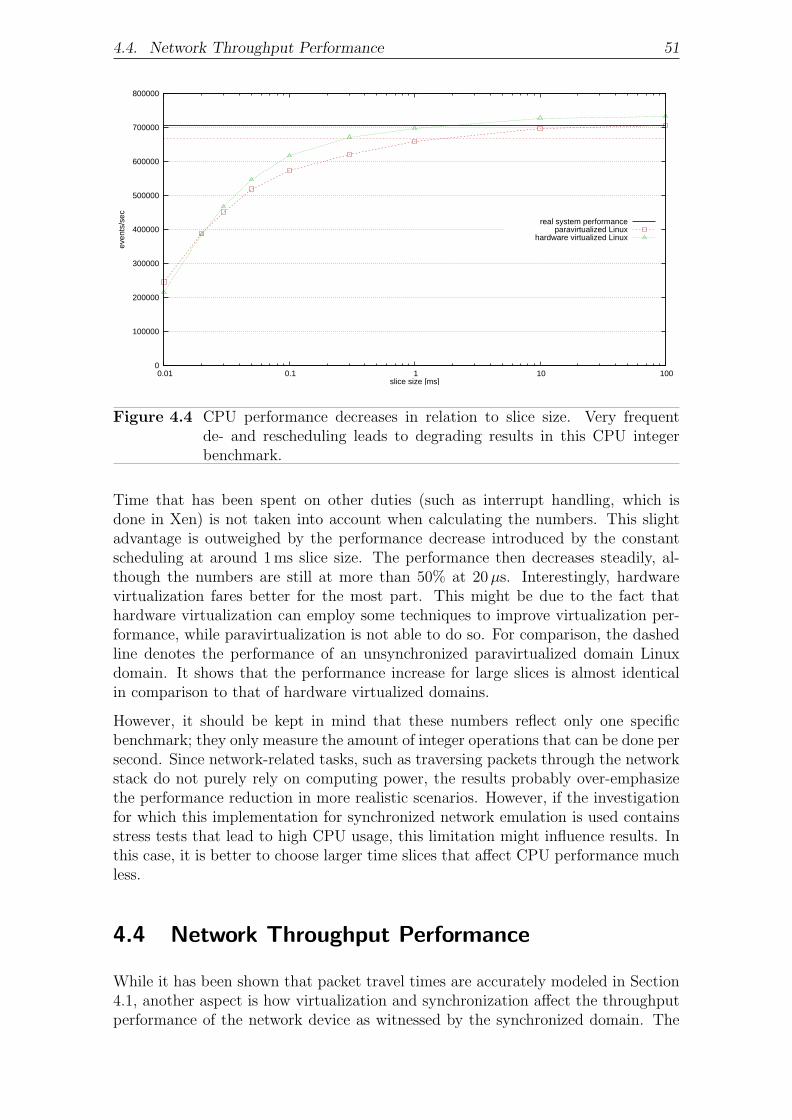
4.4. Network Throughput Performance 51

0

100000

200000

300000

400000

500000

600000

700000

800000

0.01 0.1 1 10 100

even

ts/s

ec

slice size [ms]

real system performanceparavirtualized Linux

hardware virtualized Linux

Figure 4.4 CPU performance decreases in relation to slice size. Very frequentde- and rescheduling leads to degrading results in this CPU integerbenchmark.

Time that has been spent on other duties (such as interrupt handling, which isdone in Xen) is not taken into account when calculating the numbers. This slightadvantage is outweighed by the performance decrease introduced by the constantscheduling at around 1 ms slice size. The performance then decreases steadily, al-though the numbers are still at more than 50% at 20µs. Interestingly, hardwarevirtualization fares better for the most part. This might be due to the fact thathardware virtualization can employ some techniques to improve virtualization per-formance, while paravirtualization is not able to do so. For comparison, the dashedline denotes the performance of an unsynchronized paravirtualized domain Linuxdomain. It shows that the performance increase for large slices is almost identicalin comparison to that of hardware virtualized domains.

However, it should be kept in mind that these numbers reflect only one specificbenchmark; they only measure the amount of integer operations that can be done persecond. Since network-related tasks, such as traversing packets through the networkstack do not purely rely on computing power, the results probably over-emphasizethe performance reduction in more realistic scenarios. However, if the investigationfor which this implementation for synchronized network emulation is used containsstress tests that lead to high CPU usage, this limitation might influence results. Inthis case, it is better to choose larger time slices that affect CPU performance muchless.

4.4 Network Throughput Performance

While it has been shown that packet travel times are accurately modeled in Section4.1, another aspect is how virtualization and synchronization affect the throughputperformance of the network device as witnessed by the synchronized domain. The

52 4. Evaluation

graphs in Figures 4.5 and 4.6 show results created with the netperf network per-formance benchmark [42]. Netperf consists of two pieces of software: The netperfsoftware itself is run on the computer that is benchmarked, while the netserver soft-ware is run on the machine that forms the endpoint of the network connection thatis being tested. In particular, the TCP_STREAM test was used to measure bulk TCPdata transfer rates. Computer A ran the netperf software, once on a Linux with-out Xen for comparison, and then on a paravirtualized and a hardware virtualizedLinux, respectively. The tests were done at several synchronization intervals, andunsynchronized for comparison. Computer B was running the netserver endpointsoftware for all tests. Both computers were connected directly to each other, withno network switch or any other networking hardware in between, in the same wayit was done for the timing accuracy tests.

Each netperf test at each level of synchronization, and also in the unsynchronizedcases, consisted of 12 different tests, combined from three different message sizes andfour different buffer sizes. The message sizes determine the size of the payload that isbeing sent over the network with each packet, while the socket buffer size has a directinfluence on the TCP window size. While the latter would typically be chosen by thenetwork stack and adapted to the connection speed and latency, they are set to staticvalues in these tests to analyze the network behavior in certain situations. While thismakes the tests somewhat synthetic, the choice of four different buffer sizes can giveinsight into typical as well as more extreme and rare situations. The combination ofthese two values can already have a poignant influence on the benchmark results inthe standard case on an unvirtualized Linux. Each of the 24 graphs in Figures 4.5and 4.6 depict a combination of message size, socket buffer size, and virtualizationtype (para- or hardware virtualization).

The graphs are read in the following way: Each graph has the performance of theunvirtualized Linux system in the corresponding test denoted by a black horizontalline, for comparison. For the same reason, a second, dashed horizontal line denotesthe performance of the virtualized system without any synchronization. For eachvirtualization technique, each test was run at four different time slice sizes (1 ms,300µs, 100µs and 50µs for paravirtualization, and 1 ms, 100µs, 50µs and 20µs forhardware virtualization). Those four test points are shown in the graph with their95% confidence intervals, and are connected by a dashed line.

The results are very different between para- and hardware virtualization, whichstems from the driver models used by each technique. Paravirtualization employsthe earlier mentioned “split driver” model. Here, the data that are to be sent overthe network device by the virtualized domain are simply written to a shared memoryarea, from which the privileged domain dom0, which controls the network adapter,reads the data and actually sends them. Obviously, writing to memory is much fasterthan interfacing with the network adapter, and memory is always faster by a largemargin than the network connection. Therefore, an effect that at first seems verystrange can be noticed in the netperf results for paravirtualization: with decreasingsize of the time slices that are assigned, network throughput performance increases(or rather, seems to increase from the viewpoint of the synchronized domain), to thepoint where it not only beats the performance of an unvirtualized Linux by a largemargin, but also transcends the limits of the physical line. The network throughputcan seemingly go to several Gbit/sec, which is obviously not realistic. The reasonsfor this, and possible solutions, will be discussed in Section 6.2.

4.4. Network Throughput Performance 53

0

500

1000

1500

2000

2500

3000

3500

0.05 0.3 0.1 1

netw

ork

spee

d [M

Bit/

s]

slice size [ms]

real systemparavirtualized

synchronized

(a) m = 4 kb, s = 128 kb

0

500

1000

1500

2000

2500

3000

3500

0.05 0.3 0.1 1

netw

ork

spee

d [M

Bit/

s]

slice size [ms]


synchronized

(b) m = 8 kb, s = 128 kb

0

500

1000

1500

2000

2500

3000

3500

0.05 0.3 0.1 1

netw

ork

spee

d [M

Bit/

s]

slice size [ms]


synchronized

(c) m = 32 kb, s = 128 kb

0

500

1000

1500

2000

2500

3000

0.05 0.3 0.1 1

netw

ork

spee

d [M

Bit/

s]

slice size [ms]


synchronized

(d) m = 4 kb, s = 56 kb

0

500

1000

1500

2000

2500

3000

0.05 0.3 0.1 1

netw

ork

spee

d [M

Bit/

s]

slice size [ms]


synchronized

(e) m = 8 kb, s = 56 kb

0

500

1000

1500

2000

2500

3000

0.05 0.3 0.1 1

netw

ork

spee

d [M

Bit/

s]slice size [ms]


synchronized

(f) m = 32 kb, s = 56 kb

0

500

1000

1500

2000

0.05 0.3 0.1 1

netw

ork

spee

d [M

Bit/

s]

slice size [ms]


synchronized

(g) m = 4 kb, s = 32 kb

0

500

1000

1500

2000

0.05 0.3 0.1 1

netw

ork

spee

d [M

Bit/

s]

slice size [ms]


synchronized

(h) m = 8 kb, s = 32 kb

0

500

1000

1500

2000

0.05 0.3 0.1 1

netw

ork

spee

d [M

Bit/

s]

slice size [ms]


synchronized

(i) m = 32 kb, s = 32 kb

0

200

400

600

800

1000

0.05 0.3 0.1 1

netw

ork

spee

d [M

Bit/

s]

slice size [ms]


synchronized

(j) m = 4 kb, s = 8 kb

0

200

400

600

800

1000

0.05 0.3 0.1 1

netw

ork

spee

d [M

Bit/

s]

slice size [ms]


synchronized

(k) m = 8 kb, s = 8 kb

0

200

400

600

800

1000

0.05 0.3 0.1 1

netw

ork

spee

d [M

Bit/

s]

slice size [ms]


synchronized

(l) m = 32 kb, s = 8 kb

Figure 4.5 Netperf TCP throughput performance tests for different message sizesm (option -m) and socket buffer sizes s (options -s and -S). Paravir-tualizated domain synchronized to several chosen time slices.

54 4. Evaluation

0

200

400

600

800

1000

0.02 0.05 0.01 0.1 1

netw

ork

spee

d [M

Bit/

s]

slice size [ms]

real systemhardware virtualized

synchronized

(a) m = 4 kb, s = 128 kb

0

200

400

600

800

1000

0.02 0.05 0.01 0.1 1

netw

ork

spee

d [M

Bit/

s]

slice size [ms]


synchronized

(b) m = 8 kb, s = 128 kb

0

200

400

600

800

1000

0.02 0.05 0.01 0.1 1

netw

ork

spee

d [M

Bit/

s]

slice size [ms]


synchronized

(c) m = 32 kb, s = 128 kb

0

200

400

600

800

1000

0.02 0.05 0.01 0.1 1

netw

ork

spee

d [M

Bit/

s]

slice size [ms]


synchronized

(d) m = 4 kb, s = 56 kb

0

200

400

600

800

1000

0.02 0.05 0.01 0.1 1

netw

ork

spee

d [M

Bit/

s]

slice size [ms]


synchronized

(e) m = 8 kb, s = 56 kb

0

200

400

600

800

1000

0.02 0.05 0.01 0.1 1

netw

ork

spee

d [M

Bit/

s]slice size [ms]


synchronized

(f) m = 32 kb, s = 56 kb

0

200

400

600

800

1000

0.02 0.05 0.01 0.1 1

netw

ork

spee

d [M

Bit/

s]

slice size [ms]


synchronized

(g) m = 4 kb, s = 32 kb

0

200

400

600

800

1000

0.02 0.05 0.01 0.1 1

netw

ork

spee

d [M

Bit/

s]

slice size [ms]


synchronized

(h) m = 8 kb, s = 32 kb

0

200

400

600

800

1000

0.02 0.05 0.01 0.1 1

netw

ork

spee

d [M

Bit/

s]

slice size [ms]


synchronized

(i) m = 32 kb, s = 32 kb

0

200

400

600

800

1000

0.02 0.05 0.01 0.1 1

netw

ork

spee

d [M

Bit/

s]

slice size [ms]


synchronized

(j) m = 4 kb, s = 8 kb

0

200

400

600

800

1000

0.02 0.05 0.01 0.1 1

netw

ork

spee

d [M

Bit/

s]

slice size [ms]


synchronized

(k) m = 8 kb, s = 8 kb

0

200

400

600

800

1000

0.02 0.05 0.01 0.1 1

netw

ork

spee

d [M

Bit/

s]

slice size [ms]


synchronized

(l) m = 32 kb, s = 8 kb

Figure 4.6 Netperf TCP throughput performance tests for different message sizesm (option -m) and socket buffer sizes s (options -s and -S). Hardwarevirtualized domain synchronized to several chosen time slices.

4.5. Summary 55

On the other hand, the results for hardware virtualization are somewhat impairedby the fact that a virtual network device has to be fully emulated and provided tothe hardware virtualized domain. This full emulation of a hardware device in allits details leads to results that are about 75% lower than without virtualization.2

However, the influence that synchronization has on the results is much more in linewith what one would expect: a slight decrease in performance with decreasing sizeof time slices, similar to what is witnessed for CPU performance. At this point,further analysis on several different computers to check whether CPU speed or otherfactors increase or don’t increase the network throughput for hardware virtualizeddomains compared to the unvirtualized case would provide valuable insight.

4.5 Summary

The analysis presented here shows that the modifications to the Xen hypervisorhave been successful in creating an environment that allows synchronized executionof operating systems. It also shows that there is a certain trade-off between twodifferent types of accuracy: The smaller the size of the CTW synchronization timeslices the higher the timing accuracy, but the lower the CPU performance accuracy.A user that wants to employ the synchronization system developed for this thesiswill want to run her tests at different slice sizes and compare results, or decidebeforehand about the necessary timing or CPU performance accuracy and decide ona certain size, accepting potential inaccuracies in the other area.

From the numbers presented in this chapter, it seems as if a slice size of 1ms mightbe a “sweet spot” that will be useful in many cases. The timing accuracy is highenough to produce meaningful information for most evaluation scenarios, becausefew network protocols will rely on accuracy in the sub-millisecond range. On theother hand, the CPU performance (at least the integer crunching one) is almostidentical (HVM) or at least still very close (paravirtualization) to that on a realoperating system. And finally, the overhead introduced by synchronized executionis still low. This will ensure that generally, the Xen implementation will not bethe bottleneck compared to a complex simulation. Depending on the simulationcomplexity, it will be even be possible to run several synchronized domains on onecomputer and still not bottleneck the synchronization.

Finally, network performance is still somewhat of a problem. In the hardware vir-tualized case, it behaves as one would expect it to, but performance is somewhatlow because of the necessary full emulation. In the paravirtualized case, the splitdriver model creates unrealistic results. Solutions to this problem will be discussedin Section 6.2.

2Interestingly, note how the unvirtualized system reaches its limits in throughput for smallsocket buffer sizes (8 kilobyte in the test cases). The hardware virtualized case can catch up hereand reach almost 50% of the unvirtualized performance.

56 4. Evaluation

5Related Work

This chapter will give an overview over other publications in the field of work of thisthesis. It should be noted that there is little to no work that tries to exactly achievewhat has been done in this thesis. Therefore, work related to several aspects of thisthesis are discussed one after another.

5.1 Discrete Event Simulation

The simulator used for this work is OMNeT++, in connection with the INET frame-work. As laid out in Section 2.1.1, OMNeT++ [69] is a modular discrete event sched-uler. Its simulation modules are written in C++, and can be combined to form largercompound modules, which are written in a simple script language named NED (net-work description). Nearly every part of the simulation model is easily replaceableby a custom class that serves the same purpose and has the same interface. This isdone by creating subclasses that inherit the interface from generic classes that aredelivered with OMNeT++. A good example of how expansion of OMNeT++ worksis given by the plethora of simulation models that have been developed by otherpeople for the OMNeT++ simulation system. One of those is the INET framework[38], which has been used for this work and facilitates the use of the common inter-net protocols (IP, TCP, UDP, ICMP, etc.), or the mobility framework, which allowsmodeling wireless communications of node that move in and out of communicationrange of each other.

However, there is a nearly uncountable number of network simulators in existence,even if only discrete event simulators are taken into account, including, but notlimited to ns-2 [28], parsec [8, 75], SFF [21], and JiST [10]. ns-2 was also mentionedbefore. In contrast to OMNeT++, ns-2 is more monolithic, as it brings all standardinternet protocols with it in the standard installation. As the name says (“ns” standsfor “network simulator”), it was also specifically designed for network simulation,while OMNeT++, although it is also primarily used in this area, supports additionalsimulation models due to its large amount of modularity.

58 5. Related Work

One of the developments in the simulator community is to create simulation systemsthat are programmed by the use of standard programming languages, instead ofcustom simulator languages developed for the system. The idea is that this willincrease the acceptance of new simulators in the simulation community, since userswill not have to learn a new language to use the simulator. On the other hand,those implementations have to show that they can compete in performance withsimulation systems that employ custom programming languages to drive them.

OMNeT++ goes halfways along this way: It lets the user create the basic buildingblocks, the simple modules, in the form of C++ classes, but description of compoundmodules and the overall network is done in a special, albeit very simple, descriptionlanguage. ns-2 uses C++, and network descriptions are done in Tcl which is nota language specific to ns-2, although it is not very widely used any more todayand has mostly been replaced by more powerful scripting languages. However, thesimpleness makes learning Tcl not a very time-consuming process. SFF is less asimulator than a very generic simulation framework that has to be expanded tofulfill specific roles; its minimalistic interface of a grand total of five classes and afew dozen methods is available with C++ and Java bindings. Simulators such asParsec, which was designed with parallel DES in mind, bring with them their ownspecific programming language, in the case of Parsec the homonymous programinglanguage. At the opposite end, simulation environments such as JiST go throughcomplicated steps during the compilation phase to allow using standard Java withfew limitations to write simulations models.

JiST is interesting in another aspect: The fact that it uses Java means that thecode is executed in the Java virtual machine. The idea was therefore to modify thevirtual machine in a way that lets the applications inside run in virtual time insteadof expose them to the real time of the outside world. In that way, there is an obvioussimilarity to our work, especially since the limitations placed on the Java code arerather small and often facilitate the use of already existing programs as simulationmodels with little change. However, there are certain differences that make JiSTmore limited in use. First, the fact that the changes were made to the Java virtualmachine means that it only works with Java programs. This not only rules outprototype implementations that were written in other languages, but it also meansthat it is not possible to analyze changes to the operating system kernel. Second,while our solution keeps the timing behavior of the real system intact (for the mostpart), JiST decided to forego a time model that closely resembles the original one.Instead, it mimics the behavior of more traditional simulators by enforcing that noinstruction takes any time to execute except for sleep. Therefore, the code execu-tion can be modeled by a sequence of separate events that all execute immediately,therefore creating a discrete event model. So while we brought the arbitrary startingand stopping ability of classical simulations to the prototype implementation, JiSTremoved the normal timing behavior of an application in lieu of the discrete eventtime concept of simulations.

Along a similar line, Kunz [46] presented a system that allows to plug real-world Ccode (in this case network stack code) into OMNeT++ for debugging and simulation.The C code is wrapped into C++ and converted so that for example, retransmissiontimers are modeled as self messages. As is the case with JiST, code has to fulfill afew rules so as to be convertible, and each module that is created from a predefinedblock of C code will run without any time consumption when it is called.

5.2. Opaque Network Simulation 59

Discrete event simulation systems can also be categorized by the level of detail theywork on—that is, what constitutes an event. Most of the previously mentioned sim-ulators are packet-based, so events are closely related to sending and receiving ofpackets between network nodes, and their encapsulation and decapsulation in a net-work stack. SSF, however, is generic enough not to specify what level of abstractionits simulations work on. Also JiST, as a tool which works closely on almost-stocksource code, and is not primarily concerned with network simulation, is not packet-based, but method-based: Each method forms an event that is executed at a certainpoint in virtual time, without this time progressing from instruction to instruction;events are scheduled for a future point in simulated time by calling the sleep func-tion, followed by a method call.

Since packet-based simulation models networks on a very low-level basis, and eventshave to be scheduled whenever a packet is sent, received, or processed in any way,this way of simulating networks naturally becomes computationally expensive withthe growth of the network, its complexity, and the rate at which data are exchangedbetween the nodes. A way to speed up simulation is therefore to abstract frompacket-level. One approach is to model a cluster of packets that is exchanged betweentwo nodes into a single so-called “packet train”, which reduces the number of events,as presented in [2]. Another, more radical approach is fluid-based simulation [6], inwhich the simulation model fully abstracts from single packets, and rather models therate of packets that are exchanged as a fluid flow with a given flow rate. Events arethen based on the change of the rate, and this way a single event that defines a flowcan replace thousands of events in a packet-based simulation, while still maintainingthe ability to measure many performance characteristics [54, 62]. However, fluid-based simulation is not without its own problems: An issue named the “ripple effect”[48] can massively increase the number of events, to the point where performancecan drop below that of a packet-based simulator. While there have been solutionsproposed [73], they introduce even more abstraction inaccuracies.

Moreover, all of these abstraction approaches are not useful in our field of interest.For a simulation to be able to communicate with a prototype implementation, it isnecessary that it can send replies to single packets that have been inserted into thesimulation. If it abstracts from single packets, it will not be able to communicateproperly with the prototype any more.

5.2 Opaque Network Simulation

Another set of tools has been developed to model networking behavior with a muchhigher level of abstraction than any typical discrete event simulator. These toolsdo not simulate any network nodes; rather, they only model the behavior of a linkbetween real machines that house prototype implementations. This modeling mimicstypical properties of internet connections, for example, a certain amount of link delayand limited connection speed. This approach is called “opaque network simulation”because the data packets sent through the simulator are not interpreted in any way.Each packet is seen as a black box, and the only property that can be changed isthe speed at which it is released from the application after it was received.

60 5. Related Work

It should be noted that often, this opaque network simulation is also called “net-work emulation”. While it shares this term with the network emulation that wasdescribed in Section 2.3, the two are fundamentally different. In our case, networkemulation means the translation of the representation of data from packets to simula-tor messages and vice versa, while opaque network simulation mimics (emulates) thebehavior of a long-distance connection. However, in this section, “network emulator”will be used with the meaning “opaque network simulation”.

The simplest network emulators just tap into the networking stack of the operatingsystem on which they run, and introduce an additional queue that delays packets bya predefined amount of time, and possibly randomly drops some of them. Hitbox [3]and Delayline [39] belong to this class. Slightly more complex are systems that usemultiple queues, and also model connections between them that are assigned certainproperties, such as bandwidth. Two of those network emulators are dummynet [60]and ONE [4]. Dummynet comes in the form of a patch to the FreeBSD kernel,and taps into its network stack to intercept packets. To model network routers, ituses queues in which it saves packets and keeps them for a predefined time, withthe possibility to drop a random amount of them. The link between those routersis modeled by copying packets from one inqueue to another outqueue, at a certainmaximum rate. Dummynet is used by having at least two network adapters insidethe computer it is running on, and connecting the prototypes (at least two) thatare to be tested to one of them each. All communication therefore goes through thedummynet system as a gateway, and thus facilitates the introduction of the describedeffects on every packet. ONE, the Ohio Network Emulator, works almost identically;the main difference is that it runs on Solaris, and does not require changes to theoperating system, since it runs in user space.

A newer generation of network emulators comes with additional capabilities. Forexample, NIST Net [16], developed at the National Institute of Standards and Tech-nology, a Linux kernel-based software, also facilitates packet duplication for testingscenarios, in addition to the standard delay and packet loss settings of the earlieremulators. Also, it can model the behavior of the link using trace files, that is, liverecordings of how network traffic behaved over a certain connection, and the mod-eling of congestion-dependent loss, instead of a fixed random percentage for eachpackage. In addition, it makes use of higher-resolution timer hardware in the systemit runs on, so it can control packet delay more exactly, which is very helpful withfaster connections, such as 1 GBit Ethernet.

Emusocket [7] also allows the user to set connection properties in a more detailedway than in earlier emulator software. While it does not have the advanced timerresolution capabilities of NIST Net, it has the advantage of running in user space(which is the main reason of this drawback). However, it is designed for use withJava applications only, by inserting itself into the socket API. One advantage ithas over many other emulators, such as the previously mentioned ONE, is that itis not necessary to use a dedicated computer with at least 2 network adapters touse Emusocket. Rather, all software that is to be tested can be executed on onemachine, since the network emulation work is already done at socket level.

While Emusocket allows users to run all software on one machine, RAMON [35]is a rather complicated setup consisting of software that is based on NIST Net,and dedicated hardware that is driven by the emulator. RAMON was designed

5.3. Emulation 61

to do network emulation in wireless networks and model mobility without havingto move the prototypes that are tested. To reach this goal, RAMON uses severalhardware nodes, each of which is connected to an omni-directional antenna via anattenuator and functions as an access point to the actual prototype. A controlconnection between the central network emulation entity and those nodes allows toset the signal strength and signal-to-noise ratio of the connection between them andthe prototype. By changing these two factors according to the control informationsent by RAMON, the connection can be modeled in a way that mimics mobility ofthe prototype in a wireless network. While this works well, the complex setup andnecessity of much more hardware than most other network emulators makes this acostly and somewhat complicated solution.

All in all, it has to be said that opaque network simulation excels in the area ofspeed over packet-based discrete event simulation. The fact that packets are notprocessed in any way beyond what is done in any network router facilitates muchhigher throughput through the simulation, since not every packet has to be processedthrough all network stack layers. Opaque network simulators generally are fastenough to service at least a 1 GBit ethernet connection. For comparison, NIST Netwas used with a a 200 MHz Pentium computer, and was able to cope with a saturated100 MBit link [16]. However, this abstraction means that it is not possible to modela full network with nodes that the prototype can connect to and communicate with;all of these opaque network simulators can simulate only a network connection, ora set of those, with specific behaviors. It is therefore generally necessary to have atleast two prototypes for analysis, and if more complicated network setups are to betested, the number may rise quickly. In contrast, simulators such as OMNeT++ canmodel all nodes in a network, complete with the possibility to communicate withthem, and analysis of an implementation therefore generally requires only a singleprototype in hardware if the solution presented in this thesis is used.

5.3 Emulation

The “classical” emulation, as defined in Section 2.3, is subdivided into two categoriesthat depend on how the two entities that are to be combined—that is, simulation andprototype implementation—are connected. One way is to take the software that con-stitutes the implementation, and insert it into the simulation model. This is calledenvironment emulation, or sometimes also software-in-the-loop (SiL) simulation. Inthe field of network simulation, it is often used by taking an implementation that isalready known to work, and is in widespread use, and insert it into the simulation tomake that simulation’s behavior more realistic. This has been done for the FreeBSDnetwork stack, which has been inserted into the OMNeT++ discrete event simula-tion system [14]. The “Network Simulation Cradle” [41], a wrapper that can be usedwith several different operating systems’ networking stacks (FreeBSD, OpenBSD,Linux), facilitates insertion into the ns-2 network simulator. Both of these increasethe credibility of simulation results that deal with network throughput.

This usage of environment simulation is the counterpart to what it is typically usedfor in many other fields, in which the prototype implementation is to be testedfor correct behavior. However, if the changes in the prototype implementation are

62 5. Related Work

done inside an operating system’s network stack, for example when developing anew protocol, it is possible to use an already existing environment emulation systemsuch as the ones described above, and patch the changes into the network stacksused there.

An approach that is somewhat of a hybrid between environment emulation andopaque simulation is the ENTRAPID Protocol Development Environment [36]. Run-ning in user space, it creates “virtual network kernels” (VNKs) that are based onthe FreeBSD networking stack, although the authors argue that with little work,any arbitrary network stack can be used in the same way. The stack can then bemodified for the addition and subsequent testing and analysis of newly developednetwork protocols. Every VNK can be understood as a network node, and in thisway ENTRAPID can be seen as a simulation environment, with the difference thatall nodes necessarily contain an environment emulated network stack, whereas in asimulator, one could run a subset of nodes with an integrated network stack, andsome with the simpler (and faster) standard model. To test those network stacks,application software is necessary that sends and receives data, and those are as-signed to a VNK. In this way, ENTRAPID is similar to opaque network simulation,in that no sophisticated simulation nodes exist that are simulated. Also, simulationis not event-based, but rather works with real time values. Meaningful performanceevaluation is, however, somewhat impaired by the high overhead introduced by theVNKs.

The second type of emulation as defined per Section 2.3 is network emulation, orsometimes also named “hardware-in-the-loop”. Kevin Fall was the first to presentsuch a system, which was developed for the predecessor of the ns-2 simulator, ns [27].It already contained the vital part of a network emulator: a translation unit thattransformed network packets into simulator messages, and vice versa. Despite itsage, it has (in a more recent, updated version) still been in use recently for networkemulation research, such as in [33]. Network emulation has also been used withother network simulators, such as the commercial OPNET [17] simulation system.[13] used a two-stage process, in which the communication between real systemsand their network packets, and OPNET and its message format is facilitated bytranslating both into a standardized message format that is part of the HLA (HighLevel Architecture) [23], which was specifically designed for interconnection of andcommunication between simulation systems.

For OMNeT++, the network simulator that was used in this thesis, work has recentlybeen done to create a full-fledged network emulation interface. [67] uses a translatorbetween simulation messages and network packets that is very similar to the onecreated for this thesis. However, their solution is slightly more general due to thefact that their translator does not represent every prototype implementation with acounterpoint in the simulation model. Rather, they have the translator behave likea router to the simulation, and a gateway to the prototype implementation(s). Alsocommunication between the prototype and the emulator is not done via tapped andUDP-tunneled packets, but rather by using the standard routing infrastructure ofevery network. Packet data is written using libpcap [66], which allows the gateway tosend packets that bear the addresses of the simulated hosts in their headers insteadof the gateway’s.

5.4. Encapsulation of Real Systems 63

Of the two types of emulation, environment emulation is unsuitable to reach thegoals set for this thesis. As it inserts an implementation into a network simulator,it suffers from similar problems as JiST [10], presented in Section 5.1. The imple-mentation loses its notion of wall-clock time, and instead uses the simulated timethat is presented by the simulation system. As such, while it is possible to analyzethe correct functionality, meaningful performance analysis cannot be done any more.Network emulation, on the other hand, will also be unable to produce meaningfultiming information in scenarios with complex simulations unless it employs synchro-nization. None of the solutions so far have done so, and so rely on the simulationalways being able to run in real time. While all network emulation systems presentedhere can cope with simulations that run faster than real time, none will produce use-ful results when the simulation cannot keep up with the prototype implementationsthat are connected to it. To the knowledge of the author, this thesis is the first workthat has tried to relieve simulations of this constraint.

5.4 Encapsulation of Real Systems

While virtualization and CPU emulation are both techniques that have been used fora long time, and implemented for a wide range of hardware, presented for examplein [9, 12, 20, 37, 44, 50, 72], the idea to use the encapsulation that is attained thisway for network emulation, or at least some sort of network performance analysis,is rather new, and has not found widespread use yet.

Gupta et al. presented a system in [32] that facilitates network performance evalua-tion for network speeds that are not available yet. Similar to this work, Xen is usedto encapsulate an operating system as virtualized domain, and the timekeeping sub-system is modified to achieve what the authors call “time dilation”: The illusion tothe virtualized domain that time is running slower than it actually is. This, in turn,can increase network throughput, as it appears to the domain. If a domain is runwith a time dilation factor of 10, i.e. time is passing 10 times slower inside the systemthan it does in reality, a 1 Gbit Ethernet connection may appear as a 10 Gbit one, ifit is saturated, because events arriving from outside the machine are not scaled. Toalso scale package round-trip times accordingly, dummynet [60] was used. The maindifference in how timekeeping was changed for their work and for the work presentedhere is that time is slowed down uniformly, whether the domain was scheduled ornot, and not stopped when the domain is descheduled. Also, the original systemonly supported paravirtualized domains, and did not change the scheduling subsys-tem. A follow-up publication [31] expanded on the original work by introducingmore advanced managing techniques, support for hardware virtualization, and thescaling of hard disk I/O according to the dilation factor.

Virtutech Simics [50] is a full system simulator, i.e. it emulates the behavior of aCPU, as well as all hardware devices that are connected to the simulated system. Incontrast to other CPU emulators, which often are built for a high level of accuracydown to instruction or even cycle level, Simics was designed to be a fast simulator,at least in comparison to other such applications. To reach this goal, it has to com-promise in some respects. For example, hardware emulation is transaction-based,i.e. data that are sent over the emulated network adapters are simulated not as single

64 5. Related Work

bytes sent one by one, but rather the packets form atomic units. Moreover, Simicsis only instruction accurate; it does not provide cycle accurate timing information.Simics has been used for network analysis. [26] presents a system to use Simics forevaluation of network performance of embedded devices. While Simics can simulatesystems with more computing power, full system simulation is arguably too slowto make this a worthwhile effort. The solution presented for the embedded devicesfacilitates the execution of several simulated nodes on one machine, as well as theexecution on several physical machines, which are then synchronized against eachother, much in a way that parallel distributed simulation works. While this work isvery promising, as full system simulation allows exact synchronization down to verysmall time slices, less than what is feasibly achievable with the approach presentedin this thesis (see in specific Section 4.3) and brings a full hardware emulation tothe table, the performance is very low compared to a virtualization solution. A verysimple test conducted by the author showed that a Windows XP took more than8 times as long to boot, compared to a Xen domain (335 seconds vs. 40 seconds).Furthermore, some findings suggest that Simics’ abstraction from an exact 1:1 emu-lation of x86 current processors, such as no emulation of out-of-order execution, canlead to inaccurate performance results compared to real processors [71], somethingthat one would generally not expect from a full system simulator.

5.5 Extensions to Xen

The author’s work on Xen is by far not the only extension that has been done inthe scientific community. In fact, the freely available code, its publication under theGNU General Public License, and its modular design have created possibilities tocreate a plethora of extensions that cater to different needs. A few of these will bepresented as examples in this section. It should be noted that the work done byGupta et al. [31, 32] could have also been presented in this section instead of theprevious one, since it also constitutes a Xen extension.

One of the more obvious and straightforward applications is to use Xen to debugoperating system kernels. Generally, kernel debugging is a tedious task, since thechoice of tools is limited. Separating the operating system from the hardware andthe ability to stop execution allows for more convenient debugging. A first step is touse an unmodified Xen and its already existing facilities. Kamble et al. presentedin [43] how to use Xen for Debugging kernels with gdb [30] and its gdbserver-xenextension, which is supported by any standard Xen without changes to the code.

Another step forward has been done with the creation of the Xenprobes framework[53]. Probing allows the user to set a breakpoint on any instruction in the (vir-tualized) kernel. Whenever this instruction is to be carried out, a special debuginterrupt is raised, which returns control to Xen. Xenprobes supports two types ofprobes. One is suitable for single instructions that are to be probed, by calling apre-handler and a post-handler function immediately before and after the instruc-tion is executed, respectively. The other type is used for probing function calls. Theinterrupt is set on the function entry point, and whenever the function is called, anentry-handler is executed before control returns to the function, and an exit-handlerwhen the function is about to return. The probes and their associated interrupts

5.5. Extensions to Xen 65

can be dynamically set at run time, and since each handler is a normal function,the choices of what to do when a breakpoint is reached are near limitless. A simpledebug output via printk is just as possible as incrementing counters for profiling, orsnapshots of values of certain variables.

XenAccess [55] is a tool for memory introspection (primarily; other applications,such as disk monitoring, are in development, but not as mature). It facilitates thereading of domain memory, and uses the kernel symbols to find the requested datastructures. They can then be read and presented to the user. XenAccess comeswith examples to, for example, read the current list of running processes on a Linuxkernel, or the currently loaded kernel modules, but it can be easily extended toprovide other information. Introspection is not limited to paravirtualized domains,but can also be used with hardware virtualized ones. Besides the fact that this toolfacilitates the collection of statistical data about a running system, it can also beused as an intrusion-detection system (IDS), by monitoring an operating system’ssystem call table for changes, or the integrity of kernel modules. A downside is thatXenAccess needs detailed information about the kernel memory layout of a system,so it can find the entry points for linked lists and other data structures that it wantsto introspect, so it has to be updated whenever this layout changes in a new versionof the operating system kernel.

Another very interesting extension for Xen is PTLsim/X [74], a cycle accurate fullsystem simulator that can drive a Xen domain. Its author asserts that it is the onlysuch simulator that it available as open source. It simulates a x86-64 processor,complete with modeling of pipelines and out-of-order execution. A very interestingproperty is that PTLsim can be switched between its cycle accurate mode and nativeexecution of instructions for higher speed through areas of code the user deemsuninteresting. When a domain is created, a small amount of memory is set asideto load PTLsim into it. The simulator then works as another layer of indirectionbetween the hypervisor and the domain. Because cycle accurate mode is much slowerthan native execution, livelocking due to incoming network packets poses a problem:Processing a packet will take much longer, during which several new packets mighthave arrived for processing, giving the illusion of an extremely fast network, similarto what was done on purpose in [31, 32]. Here, however, this behavior is not desired.The same can happen with other hardware devices. Therefore, PTLsim checkpointsthe system when it is set into cycle accurate mode, runs for another small amount oftime in native mode, and logs all hardware device interaction in a trace file. Then,it returns to the check point and replays the hardware events at the appropriatetime during cycle accurate simulation. The threat of livelocking is very real: Likeother cycle accurate simulators, PTLsim runs extremely slow in this mode. In a testpresented in [74], a test that took 0.7 seconds in native execution mode ran for morethan 62 minutes when done in cycle accurate mode. This means the simulation ranat less than 0.02% of real time, an overhead factor of well over 5000.

66 5. Related Work

6Future Work

In this chapter, the author wants to present a few fields of work that might benefitfrom more detailed research, analysis or further development. Three topics will bediscussed here. The first deals with how to expand synchronization onto virtualizeddomains that have been created with more than one VCPU because this case isdifferent from the uni-virtual-processor case. The second discusses solutions to theproblem of unrealistic network throughput reports in paravirtualized domains (seeSection 4.4), which can skew performance evaluation results for this virtualizationmode. Finally, the third topic discusses how to expand the synchronization systempresented in this thesis to facilitate more detailed debugging and analysis of theprototype implementations running in synchronized domains. It will propose inves-tigation into how this work can interact with XenAccess [55] and Xenprobes [53],and how these tools might benefit from each other and whether there might even bebeneficial synergy effects improving the usefulness of each tool.

6.1 Synchronizing Virtualized SMP Systems

Xen allows domains to have as many virtual CPUs as the administrator desires (up toa certain hardcoded limit, but not limited by the number of physical CPUs presentin the system). The changes to Xen done for this thesis have kept expandabilityto support for multi-VCPU domains in mind, and most of the code could actuallywork with such domains. However, some vital sections (especially the notificationfrom sEDF to the main scheduling loop that a domain has finished its assignedslice, as described in Section 3.4.1.2), will need a few more changes. The reasonthat the author has not finished the work in this area and this work has focused onsynchronizing single-VCPU domains is that synchronizing domains with more thanone VCPU creates additional, more fundamental problems in respect to timekeeping.First of all, it is important to discriminate between two cases: The number of VCPUscan either be lower than or equal to the number of physical CPUs, or it can be higher.

68 6. Future Work

(a) SMP domain in regular mode. All domains agreeon a common time base based on real time.

(b) For comparison: a one-VCPU domain in synchro-nized mode. Time only proceeds while the domain isscheduled.

(c) A synchronized SMP cannot run its VCPUs in thesame way. What time is it at the lightning mark?

(d) A solution is to always schedule all VCPUs at thesame time.

Figure 6.1 Synchronizing SMP domains creates new problems.

6.1.1 Case 1: Number of VCPUs Lower Than or Equal To Num-ber of PCPUs

When the Xen scheduler schedules a multi-VCPU domain, it makes use of its timinginformation and relays it to the domain. In other words, the domain will be able torecognize that its VCPUs do not run 100% of the time. At times, none may run, orone, or several but not all, or all of them at the same time. This is not a problembecause overall, the scheduler will ensure that the domain receives the time it wasassigned by the administrator. When a domain is assigned a certain slice of time,it will receive an overall CPU time of s · v, where s is the slice and v the number ofVCPUs. For example, a domain with 4 VCPUs and an assignment of a slice of 10 msevery 100 ms will receive 40 ms of CPU time during those 100 ms, if possible. Whenthis happens during the 100 ms period is up to the scheduler. As in the uniprocessorcase, with a standard Xen installation, domain time correlates with real time. Thisis depicted in Figure 6.1(a). Time even passes when no VCPU is running.

This way of scheduling multi-VCPU domains—that is, scheduling each VCPU in-dependent of each other—does not work for synchronized domains. There are threeconstraints that have to be met when scheduling a synchronized domain of severalVCPUs:

1. Time progresses if and only if the domain is running.

2. Time to run is assigned by the synchronization server.

6.1. Synchronizing Virtualized SMP Systems 69

3. The total CPU time is the assigned time multiplied by the number of CPUs.

If the VCPUs are simply scheduled at some point during the deadline period, timingproblems can happen, such as in Figure 6.1(c). VCPU 1 was started after VCPU 0.Time was frozen before VCPU 0 started, and then started progressing again. TheVCPUs were scheduled for 30 time units (for the sake of this example it does notmatter whether these are microseconds, milliseconds, or any time unit). After thistime, VCPU 0 is stopped, but VCPU 1 is still running. Time-wise, the domain isnow in a difficult position. What time is it at the point denoted by the lightningmark? If time continued to run, it might be around 40 time units. This, however,violates constraint 2, since the time progresses farther than the allowed 30 timeunits. Another approach would be to freeze time at 30 units. This, on the otherhand, violates constraint 1 and can lead to problems for the programs running onVCPU 1, since time calculations will be based on a time that does not progress, andtherefore invariably will be wrong. Other ideas include stopping all VCPUs whenthe assigned time has been used up (violates constraint 3), or giving each VCPU itsown time base (which again disturbs time calculations, since time might jump back-and forwards if it is compared between different VCPUs, and so violates constraint1).

This is a serious problem for synchronizing virtual SMP domains. So far, the authorhas found only one solution: All VCPUs of a domain have to be scheduled at thesame time, as depicted in Figure 6.1(d). In this case, all three constraints can beheld: Time progression coincides with running VCPUs, and the assigned time isaccurately used up, in wall clock time as well as CPU time. However, this requiresmore logistic overhead than in the single-CPU case. In detail, a close cooperation ofand communication between the schedulers running on the different physical CPUs isnecessary. Whenever a domain is scheduled, and the scheduler is called on one of thePCPUs, it has to pick a VCPU of the synchronized domain, set a flag (atomically)that represents the VCPU, signals that it is ready to be scheduled, and is readableby all the other scheduler instances. Finally, the scheduler has to spin and checkthe array until all flags are set. The next scheduler that is called has to do thesame with the next VCPU, and so on, until all VCPUs are ready to start runningimmediately. In this case, the schedulers will stop spinning, and all start schedulingthe VCPUs, all simultaneously, therefore agreeing on a common timebase. Thisis similar to how both Linux and Xen measure drift between the TSCs of differentCPU cores at system boot time on SMP systems. However, using this technique in ascheduler that is called many times per second will probably incur a very noticeableperformance decrease.

6.1.2 Case 2: Number of VCPUs Greater Than Number of PC-PUs

This case incurs even more problems than the first one. In this case, it is not possibleto use the technique described above because there are not enough physical CPUsto schedule all VCPUs at the same time. A completely new technique would benecessary. While the author, at this point in time, cannot think of any elegantsolution which would not violate one of the constraints for proper timekeeping laid

70 6. Future Work

out above, it is a field that might spur future work and will need more research anddiscussion to come to a well-founded conclusion about its feasibility. A solution tothis problem would also probably produce a more efficient solution to case 1 thanthe proposed strict simultaneous execution.

6.2 Network Throughput Performance

The analysis presented in chapter 4 has shown that for the most part, the synchro-nized execution of the virtualized operating systems works very well. However, onearea is somewhat problematic. The network throughput for paravirtualized domains(see Figure 4.5 on page 53) as it is witnessed by the synchronized domain is not re-alistic. This can be seen by the fact that a TCP throughput benchmark reportsnumbers as high as 3 GBit/s on a network adapter that only supports a maximumof 1 GBit/s. This is due to Xen’s “split driver” model. The paravirtualized domainuses a very simple network driver front-end, which does not interact with the hard-ware at all, and rather puts data it wants to send out into a shared memory area.The dom0 contains the actual driver back-end that interfaces with the hardware,and will take the data out of the shared memory to send packets on behalf of theunprivileged domains.

Obviously, writing data into memory is a much faster operation than sending datato the network adapter. The synchronized domain therefore can put more datainto the shared memory than it would be able to send to the network adapter, ifit had direct access to it, up to the point of completely filling the shared memory.Whenever the domain is descheduled, the control domain dom0 starts to empty theshared memory buffer and send the packets over the wire. This happens while thesynchronized domain is descheduled, and therefore during a time that it doesn’trealize is passing at all. Since the dom0 is running much more often in between thesynchronized domain for smaller time slices, this explains the seemingly increasingspeed with decreasing slice size.

A solution to this is to change the back-end network driver in the privileged do-main dom0 to be aware of the synchronization of domains that it sends and receivedpackets on behalf of. Thus, a synchronized driver would send only the appropriateamount of data to the network adapter whenever a synchronized domain is desched-uled. For example, if the size of the time slices was set to 100µs, and the networkadapter is a 100 MBit Ethernet device, the maximum amount of data to be sentwould be 1250 bytes. Packets are sent out until this margin is reached.

Another way to tackle this problem could be to investigate PTLsim’s [74] capabil-ities at doing a full emulation of hardware devices. Then again, the cycle accurateexecution entails a crippling speed penalty which in all likelihood rules out thisapproach.

Finally, it should be noted that fully emulated drivers in hardware virtualized modedo not produce paradoxical results for network throughput performance, but ratherbehave as expected. However, network throughput is noticeably lower than on anunvirtualized system. If one found a solution to synchronize the paravirtualizedback-end driver, it would be possible to eventually use special drivers in the hard-ware virtualized domain that take advantage of the knowledge that their operating

6.3. Introspection and Probing 71

system is virtualized. Such paravirtualized drivers for hardware virtualized domainshave been in development for some time—for example, for Windows XP [34]. Thisway, the network throughput performance of hardware virtualized domains could beincreased, and a combination of high performance and meaningful results could bereached.

6.3 Introspection and Probing

This work presents a set of tools that facilitates synchronization of an operatingsystem with a prototype implementation to a packet-based discrete event simulator.One of the reasons for this was to lower the requirements for prototype analysis byusing only one prototype together with a simulated network, instead of a testbed ofmany prototypes. In addition, it is much faster and easier to restructure a simulatednetwork inside a simulation than it is to reorganize a network testbed constructedfrom real machines.

Another step forward in this field of both detailed and convenient analysis wouldbe to expand the Xen implementation to make debugging potential software errorseasier, while the prototype is running inside a Xen domain. Section 5.5 presentedtwo extensions to Xen that can aid the user in debugging, namely XenAccess [55] andXenprobes [53]. XenAccess allows introspection into the memory of a domain thatis currently running, and Xenprobes places hook functions on instructions. Each ofthese tools on its own is already a helpful aid in analysis and debugging. Combined,and with the synchronization presented in this thesis, they can form a powerfulcombination for development and analysis. It would be possible to read the contentsand state of the networking stack of a synchronized operating system via XenAccesswhenever an assigned time slice has ended, or to probe certain functions in the codethat was added.

While both tools introduce a considerable overhead and therefore slow down theexecution, synchronization as presented in this thesis will ensure that the results arevery close to the behavior of the uninstrumented system in regards to time behavior.1

While the machine that Xen and the synchronized domain are executed on will takelonger to execute one time slice, we have shown in Chapter 4 that time warpingas presented in Section 3.4.2 accomplishes requirement 2 as set in the introduction.Therefore, time spent outside of the synchronized domain—that is, in XenAccessor Xenprobes—will not be attributed to the synchronized domain; the additionaloverhead that is created is only a nuisance, but it will not influence the results inany clearly noticeable way.

The next steps in this direction could be to test how well XenAccess and Xenprobeswork together with the current version of Xen, and the synchronization changes.Then, XenAccess would have to be extended to read network stack status, andmake it executable from either the Xen kernel or the dom0 kernel, so that it could becalled automatically whenever a synchronized domain has finished running its timeslice. Since XenAccess runs inside the privileged domain dom0, the timewarping

1In theory, the only differences will be due to more context switches between synchronizeddomain and Xen/dom0, and performance decreases due to cache misses and pipeline stalls. Theeffects of this can be seen in Figure 4.4 and page 51.

72 6. Future Work

code should work with it without any changes. For Xenprobes to work properly,a small change to the debug interrupt’s handler will be necessary, so as to stopthe synchronized domains time while the interrupt is being serviced; this way, theinterrupt handling will not be realized by the domain due to lost time.

7Conclusion

This diploma thesis presented network emulation, that is, the connection of a realsystem running a prototype implementation with a network simulator, and focusedon a specific problem of this field: The fact that while both have a notion of time,its representation is fundamentally different in a simulator and a real system onx86 hardware. It was shown that problems occur when these two representationsof time do not agree on the current time. So far, this problem had generally beensolved by using simulation systems on very fast hardware, or distributing them overseveral machines, to ensure that they will never be slower than real time, even invery complex simulation, and then slow them down to real time when they are faster.This ensured that simulation time would run in unison with real time, which is thebasis of the clocks inside a hardware prototype.

However, the underlying problem is that it is not always possible to make a simula-tion fast enough to meet the goal of real time capability. For every system, no matterits number-crunching ability, there are simulations complex enough to slow it downso that this capability is lost. Therefore, this diploma thesis presented a way toslow down the real system that is connected in the network emulation scenario, andexecute its operating system synchronously to the simulation, so that the real-timeconstraint is lifted from the simulation.

To reach this goal, the Xen Hypervisor was used to encapsulate the real systeminside a virtual machine, so as to detach it from the hardware it would otherwiserun on, while keeping all of the internal behavior intact, so that results from runningthe prototype implementation are credible. Two fields of work were identified tofacilitate synchronous execution. First, Xen’s scheduling subsystem was modified sothat it allowed precise scheduling on demand of a virtualized OS for short amounts oftime. This made it possible to have a real system wait on the simulator whenever thelatter fell behind because it could not run in real time. Second, the interface betweenthe OS and the hardware clocks that define its timing behavior was modified to maskpassing of time while the OS is descheduled, so that the illusion of a continuous flowof time is upheld. This way, an operating system could be stopped for arbitraryamounts of time, without the OS ever noticing it was stopped.

74 7. Conclusion

A detailed insight into how these changes were implemented was given in Chapter 3.Changes to the scheduling subsystem involved modifying the Xen sEDF scheduler,but also the main scheduling loop, to make it aware of time it consumed itselfduring the scheduling. Changes to the timekeeping subsystem had to be done forboth paravirtualized and hardware virtualized Xen domains, and involved using timeinformation created by the scheduler and by Xen’s own timekeeping facilities to stoptimers that signaled the passing of time, and warp them and time counters in properways to keep up the illusion of a continuous flow of time to the Xen domain.

To construct a fully working setup in which synchronized network emulation couldbe used and its correct functionality be analyzed, a set of tools was developed andimplemented besides the Xen modifications. First of all, a central synchronizationserver was necessary that kept a reference clock and instructed simulation and proto-type to run for specified amounts of time, implementing a conservative time windowsalgorithm (see Section 2.4). It was also necessary to create a client that ran on theXen machine and formed an interface between the synchronization server and themodified Xen. Finally, an emulator had to be constructed that made communicationbetween simulation and prototype possible.

When the work for this thesis was started, it was not clear whether an approach tosynchronized network emulation using the Xen Hypervisor was feasible at all. The re-sults of the analysis presented in Chapter 4 showed that the solution presented worksvery well, providing a synchronization accuracy of down to 10µs. Furthermore, atlarger time slices that are nevertheless still useful for network protocol analysis in anetwork emulation scenario, the overhead introduced by the synchronization is verylow, less than 50% at an accuracy of 100µs, and less 25% for hardware virtualizationand 6% for paravirtualization for an accuracy of 1 ms. Finally, the timing resultsmeasured are very comparable between a network emulation setup with a simulationthat is not real time capable, and a setup consisting of two real systems. This meansthat the solution presented in this thesis can be used for detailed and meaningfulanalysis with simulations of arbitrary complexity, relieving network emulation of itsconstraint of real time capable network simulations.

The main problem with the implementation at this point in time is that, for operatingsystems virtualized via paravirtualization, network throughput results measured inthe virtualized operating system are not credible. Suggestions on how to solve thisproblem were proposed in Section 6.2. The author assumes that a solution will notonly be possible, but also realizable with relatively little investment of time andwork.

Finally, while this work has focused on using synchronization of operating systemsfor synchronized network emulation, a fundamentally new field of application opensup when it is combined with tools for introspection and probing. As has beendescribed in detail in Section 6.3, a combination of this work’s synchronization withXenAccess and Xenprobes will allow to debug an operating system with convenientand powerful tools, while at the same time keeping its timing behavior intact. Whilegenerally, debugging introduces new delays, and breakpoints set for this purposecan totally change the timing behavior, synchronization will mask the time spent indebugging functions from the debugged operating system. This will allow to debuga system that behaves as if it was running without any debugging action, even intime-sensitive areas of the implementation.

75

Therefore, the author not only concludes that synchronization of operating systemscreated a system for feasible and powerful network analysis through synchronizednetwork emulation, but he also anticipates exciting new use cases in the field ofoperating system debugging.

76 7. Conclusion

Bibliography

[1] Adair, R. J., Bayles, R. U., Comeau, L. W., and Creasy, R. J. Avirtual machine system for the 360/40. Tech. rep., Cambridge Scientific CenterReport 320-2007, 1966.

[2] Ahn, J. S., and Danzig, P. B. Packet network simulation: speedup andaccuracy versus timing granularity. IEEE/ACM Transactions on Networking(TON) 4, 5 (1996), 743–757.

[3] Ahn, J. S., Danzig, P. B., Liu, Z., and Yan, L. Evaluation of TCPvegas: emulation and experiment. In SIGCOMM ’95: Proceedings of the con-ference on Applications, technologies, architectures, and protocols for computercommunication (New York, NY, USA, 1995), ACM, pp. 185–195.

[4] Allman, M., Caldwell, A., and Ostermann, S. ONE: The ohio networkemulator. Tech. Rep. TR-19972, School of Electrical Engineering and ComputerScience, Ohio University, August 1997.

[5] AMD. AMD64 Virtualization Codenamed ”Pacifica Secure” Virtual MachineArchitecture Reference Manual. AMD, May 2005.

[6] Anick, D., Mitra, D., and Sondhi, M. M. Stochastic theory of a datahandling system with multiple sources. In ICC ’80: International Conferenceon Communications (June 1980), pp. 13.1.1–13.1.5.

[7] Avvenuti, M., and Vecchio, A. Application-level network emulation: theemusocket toolkit. Journal of Network and Computer Applications 29, 4 (2006),343–360.

[8] Bagrodia, R., Meyer, R., Takai, M., an Chen, Y., Zeng, X., Martin,J., and Song, H. Y. Parsec: A parallel simulation environment for complexsystems. Computer 31, 10 (1998), 77–85.

[9] Barham, P., Dragovic, B., Fraser, K., Hand, S., Harris, T., Ho,A., Neugebauer, R., Pratt, I., and Warfield, A. Xen and the art ofvirtualization. In SOSP ’03: Proceedings of the nineteenth ACM ymposium onOperating systems principles (New York, NY, USA, 2003), ACM, pp. 164–177.

[10] Barr, R., Haas, Z. J., and van Renesse, R. JiST: an efficient approachto simulation using virtual machines. Software—Practice and Expererience 35,6 (2005), 539–576.

78 Bibliography

[11] Baumgart, I., Heep, B., and Krause, S. OverSim: A flexible overlaynetwork simulation framework. In 10th IEEE Global Internet Symposium (May2007), pp. 79–84.

[12] Bellard, F. QEMU, a fast and portable dynamic translator. In ATEC ’05:Proceedings of the USENIX Annual Technical Conference (Berkeley, CA, USA,2005), USENIX Association, pp. 41–41.

[13] Biegeleisen, E., Eason, M., Michelson, C., and Reddy, R. Network inthe loop using HLA, distributed OPNET simulations, and 3D visualizations. InMILCOM ’05: Proceedings of the IEEE Military Communications Conference(October 2005), vol. 3, pp. 1667–1671.

[14] Bless, R., and Doll, M. Integration of the FreeBSD TCP/IP-stack intothe discrete event simulator OMNeT++. In Proceedings of the 2004 WinterSimulation Conference (2004), Winter Simulation Conference, pp. 1556–1561.

[15] Buttazzo, G. C. Rate monotonic vs. EDF: judgment day. Real-Time Systems29, 1 (2005), 5–26.

[16] Carson, M., and Santay, D. NIST net: a linux-based network emulationtool. ACM SIGCOMM Computer Communication Review 33, 3 (2003), 111–126.

[17] Chang, X. Network simulations with OPNET. In Proceedings of the 1999Winter Simulation Conference (1999), vol. 1, pp. 307–314.

[18] Chisnall, D. The Definitive Guide to the Xen Hypervisor. Prentice Hall,Upper Saddle River, New Jersey, USA, 2007.

[19] Chun, B., Culler, D., Roscoe, T., Bavier, A., Peterson, L., Wawr-zoniak, M., and Bowman, M. PlanetLab: an overlay testbed for broad-coverage services. SIGCOMM Comput. Commun. Rev. 33, 3 (2003), 3–12.

[20] Corbato, F. J., Merwin-Daggett, M., and Daley, R. C. An exper-imental time-sharing system. In AFIPS Conference Proceedings: 1962 SpringJoint Computer Conference (1962), vol. 21, pp. 335–344.

[21] Cowie, J. H., Nicol, D. M., and Ogielski, A. T. Modeling the globalinternet. Computing in Science and Engineering 1, 1 (1999), 42–50.

[22] Creasy, R. J. The origin of the VM/370 time-sharing system. IBM Journalof Research and Development 25, 5 (September 1981), 483–490.

[23] Dahmann, J. S. Standards for simulation: As simple as possible but notsimpler—high level architecture for simulation. In DIS-RT ’97: Proceedings ofthe 1st International Workshop on Distributed Interactive Simulation and Real-Time Applications (Washington, DC, USA, 1997), IEEE Computer Society.

[24] Diestelhorst, S. Scheduling operating-systems. Studienarbeit, TechnicalUniversity Dresden, June 2007.

Bibliography 79

[25] Drytkiewicz, W., Sroka, S., Handziski, V., Kopke, A., and Karl,H. A mobility framework (MF) for OMNeT++. In Proceedings of the ThirdInternational OMNeT++ Workshop (2003).

[26] Engblom, J., Kagedal, D., Moestedt, A., and Runeson, J. Develop-ing embedded networked products using the simics full-system simulator. InPIMRC ’05: Proceedings of the Sixteenth IEEE International Symposium onPersonal, Indoor and Mobile Radio Communications (September 2005), vol. 2,pp. 785–789.

[27] Fall, K. Network emulation in the Vint/NS simulator. In Proceedings ofthe Fourth IEEE International Symposium on Computers and Communications(1999), pp. 244–250.

[28] Fall, K., and Varadhan, K. The network simulator ns-2.http://www.isi.edu/nsnam/ns/.

[29] Fujimoto, R. M. Parallel discrete event simulation. Communications of theACM 33, 10 (1990), 30–53.

[30] GDB: The GNU debugger project. http://www.gnu.org/software/gdb/.

[31] Gupta, D., Vishwanath, K. V., and Vahdat, A. DieCast: Testing dis-tributed systems with an accurate scale modeling. In NSDI ’08: 5th USENIXSymposium on Networked Systems Design and Implementation (Aprilx 2008).

[32] Gupta, D., Yocum, K., Yocum, K., McNett, M., Snoeren, A. C.,Vahdat, A., and Voelker, G. M. To infinity and beyond: time warpednetwork emulation. In SOSP ’05: Proceedings of the Twentieth ACM Sympo-sium on Operating Systems Principles (New York, NY, USA, 2005), ACM.

[33] Guruprasad, S., Ricci, R., and Lepreau, J. Integrated network experi-mentation using simulation and emulation. In TRIDENTCOM ’05: Proceedingsof the First International Conference on Testbeds and Research Infrastructuresfor the DEvelopment of NeTworks and COMmunities (Washington, DC, USA,2005), IEEE Computer Society, pp. 204–212.

[34] Harper, J., and Grover, A. GPL paravirtualized drivers for windows.http://xenbits.xensource.com/ext/win-pvdrivers.hg.

[35] Hernandez, E., and Helal, A. S. RAMON: Rapid-mobility network emu-lator. In LCN ’02: Proceedings of the Twenty-Seventh Annual IEEE Conferenceon Local Computer Networks (Washington, DC, USA, 2002), IEEE ComputerSociety, pp. 809–820.

[36] Huang, X., Sharma, R., and Keshav, S. The ENTRAPID protocol devel-opment environment. In INFOCOM ’99: Proceedings of the Eighteenth AnnualJoint Conference of the IEEE Computer and Communications Societies (March1999), vol. 3, pp. 1107–1115.

[37] Hwang, J.-Y., Suh, S.-B., Heo, S.-K., Park, C.-J., Ryu, J.-M., Park,S.-Y., and Kim, C.-R. Xen on ARM: System virtualization using xen hy-pervisor for ARM-based secure mobile phones. In CCNC 2008: Proceesings of

http://www.isi.edu/nsnam/ns/

http://www.gnu.org/software/gdb/

http://xenbits.xensource.com/ext/win-pvdrivers.hg

80 Bibliography

the Fifth IEEE Consumer Communications and Networking Conference (2008),pp. 257–261.

[38] The INET framework for OMNeT++. http://www.omnetpp.org/

staticpages/index.php?page=20041019113420757.

[39] Ingham, D. B., and Parrington, G. D. Delayline: a wide-area networkemulation tool. Computing Systems 7, 3 (1994), 313–332.

[40] Intel. IA-PC HPET (high precision event timers) specification.http://www.intel.com/hardwaredesign/hpetspec_1.pdf, October 2004.

[41] Jansen, S., and McGregor, A. Simulation with real world network stacks.In Proceedings of the 2005 Winter Simulation Conference (2005).

[42] Jones, R. The netperf benchmark. http://www.netperf.org.

[43] Kamble, N. A., Nakajima, J., and Mallick, A. K. Evolution in kerneldebugging using hardware virtualization with xenprobes. In Proceedings of the2006 Linux Symposium (July 2006).

[44] Kivity, A., Kamay, Y., Laor, D., Lublin, U., and Liguori, A. kvm:The linux virtual machine monitor. In Proceedings of the 2007 Linux Symposium(Ottawa, August 2007).

[45] Krasnyansky, M. Universal TUN/TAP driver.http://vtun.sourceforge.net/tun/.

[46] Kunz, G. Entwurf und Implementierung einer PlattformabstraktionsschIchtfur modulare Kommunikationsprotokolle. Diplomarbeit, RWTH Aachen Uni-versity, December 2007.

[47] Lawton, K. P. Bochs: A portable PC emulator for Unix/X. Linux Journal29 (1996), article no.7.

[48] Liu, B., Figueiredo, D., Guo, Y., Kurose, J., and Towsley, D. Astudy of networks simulation efficiency: fluid simulation vs. packet-level simu-lation. In INFOCOM 2001: Proceedings of the Twentieth Annual Joint Con-ference of the IEEE Computer and Communications Societies (2001), vol. 3,pp. 1244–1253.

[49] Liu, C. L., and Layland, J. W. Scheduling algorithms for multiprogram-ming in a hard-real-time environment. Journal of the ACM 20, 1 (1973), 46–61.

[50] Magnusson, P. S., Christensson, M., Eskilson, J., Forsgren, D.,Hallberg, G., Hogberg, J., Larsson, F., Moestedt, A., andWerner, B. Simics: A full system simulation platform. Computer 35, 2(2002), 50–58.

[51] Misra, J. Distributed discrete-event simulation. ACM Computing Surveys 18,1 (1986), 39–65.

http://www.omnetpp.org/staticpages/index.php?page=20041019113420757

http://www.omnetpp.org/staticpages/index.php?page=20041019113420757

http://www.intel.com/hardwaredesign/hpetspec_1.pdf

http://www.netperf.org

http://vtun.sourceforge.net/tun/

Bibliography 81

[52] Nakajima, J., Mallick, A., Pratt, I., and Fraser, K. x86-64 XenLinux:Architecture, implementation, and optimizations. In Proceedings of the 2006Linux Symposium (Ottawa, August 2006).

[53] Nguyen, A. Q., and Suzaki, K. Xenprobes, a lightweight user-space probingframework for xen virtual machine. In ATEC ’07: Proceedings of the 2007USENIX Annual Technical Conference (June 2007), pp. 15–28.

[54] Nicol, D., Goldsby, M., and Johnson, M. Fluid-based simulation ofcommunication networks using SSF. In Proceedings of the 1999 European Sim-ulation Symposium (October 1999).

[55] Payne, B., de Carbone, M., and Lee, W. Secure and flexible monitoringof virtual machines. In ACSAC ’07: Twenty-Third Annual Computer SecurityApplications Conference (December 2007), pp. 385–397.

[56] Popek, G. J., and Goldberg, R. P. Formal requirements for virtualizablethird generation architectures. Communications of the ACM 17, 7 (1974), 412–421.

[57] Postel, J. RFC 792: Internet control message protocol.http://www.ietf.org/rfc/rfc0792.txt, September 1981.

[58] Pratt, I., Fraser, K., Hand, S., Limpach, C., Warfield, A., Ma-genheimer, D., Nakajima, J., and Mallick, A. Xen 3.0 and the art ofvirtualization. In Proceedings of the Seventh Linux Symposium (July 2005),vol. 2, pp. 65–77.

[59] Riedl, J. Time and packet synchronization of the OMNeT++ simulator.Studienarbeit, University of Tubingen, August 2005.

[60] Rizzo, L. Dummynet: a simple approach to the evaluation of network proto-cols. ACM SIGCOMM Computer Communication Review 27, 1 (1997), 31–41.

[61] Robin, J. S., and Irvine, C. E. Analysis of the intel pentium’s abilityto support a secure virtual machine monitor. In SSYM’00: Proceedings ofthe Ninth USENIX Security Symposium (Berkeley, CA, USA, 2000), USENIXAssociation, pp. 10–25.

[62] Ros, D., and Marie, R. Estimation of end-to-end delay in high-speed net-works by means of fluid model simulation. In Proceedings of the ThirteenthEuropean Simulation Multiconference (June 1999).

[63] Rosenblum, M., and Garfinkel, T. Virtual machine monitors: currenttechnology and future trends. Computer 38, 5 (May 2005), 39–47.

[64] Sites, R. L., Chernoff, A., Kirk, M. B., Marks, M. P., and Robin-son, S. G. Binary translation. Communications of the ACM 36, 2 (1993),69–81.

[65] Strachey, C. Time sharing in large fast computers. In Proceedings of theInternational Conference on Information Processing (1959).

[66] TCPDUMP/LIBPCAP public repository. http://www.tcpdump.org.

http://www.ietf.org/rfc/rfc0792.txt

http://www.tcpdump.org

82 Bibliography

[67] Tuxen, M., Rungeler, I., and Rathgeb, E. P. Interface connecting theINET simulation framework to the real world. In SIMUTools ’08: Proceedingsof the First International Conference on Simulation Tools and Techniques forCommunications, Networks and Systems (March 2008).

[68] Uhlig, R., Neiger, G., Rodgers, D., Santoni, A. L., Martins, F.C. M., Anderson, A. V., Bennett, S. M., Kagi, A., Leung, F. H.,and Smith, L. Intel virtualization technology. Computer 38, 5 (2005), 48–56.

[69] Varga, A. The OMNeT++ discrete event simulation system. In ESM ’01:Proceedings of the European Simulation Multiconference (June 2001).

[70] Varian, M. VM and the VM community: Past, present, and future.http://www.princeton.edu/~melinda/25paper.pdf, 1997.

[71] Villa, F. J., Acacio, M. E., and Garcıa, J. M. Evaluating IA-32 webservers through simics: a practical experience. Journal of Systems Architecture51, 4 (2005), 251–264.

[72] VMWare homepage. http://www.vmware.com.

[73] Yan, A., and Gong, W.-B. Time-driven fluid simulation for high-speednetworks. IEEE Transactions on Information Theory 45, 5 (July 1999), 1588–1599.

[74] Yourst, M. PTLsim: A cycle accurate full system x86-64 microarchitecturalsimulator. In ISPASS ’07: Proceedings of the IEEE International Symposiumon Performance Analysis of Systems & Software (April 2007), pp. 23–34.

[75] Zeng, X., Bagrodia, R., and Gerla, M. Glomosim: a library for parallelsimulation of large-scale wireless networks. In PADS ’98: Proceedings of theTwelfth Workshop on Parallel and Distributed Simulation (May 1998), pp. 154–161.

http://www.princeton.edu/~melinda/25paper.pdf

http://www.vmware.com

ASynchronization System Setup

This appendix will give a more comprehensive overview over what configuration op-tions exist for the different programs that together form the synchronization systemdeveloped for this thesis, and how to set up synchronized network emulation betweenan OMNeT++ simulation and a Xen domain.

A.1 Configuration Options

A.1.1 Stand-Alone Synchronization Server

The stand-alone synchronization server is a user-space application that is configuredvia its configuration file config.sync which the server expects to be in the samedirectory as the executable. It is in a standard INI file format, i.e. it consists ofsections that contain variables and their assignments. Note that while the servercomes with some rudimentary support functionality to run as client, there is littleuse for this feature at this point in time, as it can interface with neither Xen norOMNeT++ in this function. Consequently, this setup has not been tested.

84 A. Synchronization System Setup

Section Name DescriptionGENERAL mode “client” or “server”

SERVER

srv barrier interval An integer that sets the size of a CTW syn-chronization time slice, in µs.

srv brdcast address The IP broadcast address of the network, indotted decimal notation.

server port The port the server listens on.

CLIENT

client id A numerical identifier for the client. Mustbe unique over all clients participating in thesynchronization.

client type An identifier that can describe the type ofclient.

client sync server The IP address of the server the client willconnect to, in dotted decimal notation.

client port The port the client listens on, i.e. the port onwhich the broadcast run messages are sent.

A.1.2 Xen Synchronization Client

The Xen synchronization client comes in the form of a kernel module. All options arepassed on the command line, or can optionally be added to the module options file.The location of this file depends on the used Linux distribution, but a typical locationis /etc/modprobe.d/options. Note that the option to use the kernel module assynchronization server was not thoroughly tested.

Name Type Descriptionrun as server int If set to 1, allows the module to function as server

instead of client.server address char[] The IP address of the server, in dotted decimal no-

tation.server port int The port the synchronization server listens on.broadcast address char[] The IP broadcast address of the network, in dotted

decimal notation.client port int The port the client listens on, i.e. the port on which

the broadcast run messages are sent.cli id int A numerical identifier for the client. Must be unique

over all clients participating in the synchronization.cli descr char[] A description string that can be used to identify the

client at the server.sync domain int[] A comma-separated list of domains that are to be

synchronized on this machine.barrier time int In server mode: the size of a CTW synchronization

time slice.

A.1.3 OMNeT++ Synchronization Client–Scheduler

The synchronization client written for OMNeT++ is part of the scheduler thatdrives the simulator according to the assigned time slices (see Section 3.2.2 for more

A.1. Configuration Options 85

information). As such, it is configured the same way as any other OMNeT++component, i.e. by setting the options in the omnetpp.ini file that belongs to thesimulation model. First of all, the option scheduler-class has to be set to cSync-

Scheduler in the General section. The other options are set in a section namedSync.

Name Type Descriptionsync enabled boolean If “no”, the scheduler will not be synchronized and

work like a normal scheduler.client id int A numerical identifier for the client. Must be unique

over all clients participating in the synchronization.client description string A description string that can be used to identify the

client at the server.sync server string The IP address of the server, in dotted decimal no-

tation.sync server port int The port the synchronization server listens on.sync client port int The port the synchronization client listens on.debug boolean If “yes”, print debugging information to STDOUT

while running.sync unit scaler double A scale factor. The time slice that is received from

the server is divided by this number. Since the syn-chronization server described in Section A.1.1 sendsthe time in µs, but OMNeT++ expects the time inseconds, it is set to 1000000 and should generallynot be changed.

A.1.4 Emulator–Tunnel: Xen Side

The tunnel is set up by an application tap-udptunnel that expects three commandline options: First, the IP address of the endpoint of the tunnel, i.e. the computerthe simulation is running on. Second, a part number of the endpoint. Third, aflow-id that uniquely identifies this tunnel. If there are several Xen hosts connectedto the simulation, they will all share the IP address and port endpoints, but theywill each receive a unique flow-id. As next step, a new bridge has to be created,and the virtual interface vifN.0 corresponding to the synchronized domain has tobe bridged with the tap devices that was created by starting the tap-udptunnel

program. Finally, ARP has to be switched off on the bridge.

A.1.5 Emulator–Tunnel: OMNeT++ Side

The configuration options are spread over two files. The general options are set inthe omnetpp.ini file, in a section named cExternal-Tunnel.

86 A. Synchronization System Setup

Name Type Descriptiontunnel enabled boolean If “no”, no functional coupling will take place.

Consequently, no communication between simula-tion and Xen domain will be possible.

tunnel destination string The IP address of the endpoint of the tunnel, indotted decimal notation.

tunnel port int The port of the endpoint of the tunnel.

The flow-id, which uniquely identifies each Xen domain’s traffic, is set in the networkdescription file. Since each Xen domain is identified with a network node of the typecExtHost inside the simulation (see Section 3.3), the flow-id is set as one of itsparameters with the name flowid and an integer as value.

A.2 Synchronized Network Emulation Setup

1. Boot one computer into Xen, and one computer into Linux.

2. Start the domain that is to be synchronized on the Xen computer.

3. Start the tap-udptunnel script on the Xen computer.

4. Bridge the virtual interface that belongs to the domain that is to be synchro-nized with the newly created tap device. Do not forget to switch off ARP onthe bridge.

5. Start the synchronization server on the Linux computer (or the Xen computer,or any other third computer).

6. Start OMNeT++ on the Linux computer.

7. Load the kernel module on the Xen machine.

8. Start the OMNeT++ simulation.

synchronization of operating systems in … of operating systems in heterogeneous testing...

Documents