synchronization of oscillators in a kuramoto-type model ...pikovsky/pdffiles/2014/chaos_14... ·...
TRANSCRIPT
Synchronization of oscillators in a Kuramoto-type model with genericcoupling
Vladimir Vlasov1a) Elbert E N Macau2 and Arkady Pikovsky13
1Department of Physics and Astronomy Potsdam University 14476 Potsdam Germany2National Institute for Space Research - INPE 12227-010 Sao Jose dos Campos SP Brazil3Department of Control Theory Nizhni Novgorod State University Gagarin Av 23 606950Nizhni Novgorod Russia
(Received 28 March 2014 accepted 19 May 2014 published online 30 May 2014)
We study synchronization properties of coupled oscillators on networks that allow description in
terms of global mean field coupling These models generalize the standard KuramotondashSakaguchi
model allowing for different contributions of oscillators to the mean field and to different forces from
the mean field on oscillators We present the explicit solutions of self-consistency equations for the
amplitude and frequency of the mean field in a parametric form valid for noise-free and noise-driven
oscillators As an example we consider spatially spreaded oscillators for which the coupling
properties are determined by finite velocity of signal propagation VC 2014 AIP Publishing LLC
[httpdxdoiorg10106314880835]
Synchronization of large ensembles of oscillators is an
ubiquitous phenomenon in physics engineering and life
sciences The most simple setup pioneered by Winfree
and Kuramoto is that of global coupling where all the
oscillators equally contribute to a mean field which acts
equally on all oscillators In this study we consider a gen-
eralized Kuramoto-type model of mean field coupled
oscillators with different parameters for all elements In
our setup there is still a unique mean field but oscillators
differently contribute to it with their own phase shifts
and coupling factors and also the mean field acts on each
oscillator with different phase shifts and coupling coeffi-
cients Additionally the noise term is included in the con-
sideration Such a situation appears eg if the oscillators
are spatially arranged and the phase shift and the attenu-
ation due to propagation of their signals cannot be
neglected A regime where the mean field rotates uni-
formly is the most important one For this case the solu-
tion of the self-consistency equation for an arbitrary
distribution of frequencies and coupling parameters is
found analytically in the parametric form both for noise-
free and noisy oscillators First we consider independent
distributions for the coupling parameters when self-
consistency equations can be greatly simplified Second
we consider an example of a particular geometric organi-
zation of oscillators with one receiver that collects signals
from oscillators and with one emitter that sends the driv-
ing field on them By using our approach synchroniza-
tion properties can be found for different geometric
structures andor for different parameter distributions
I INTRODUCTION
Kuramoto model of globally coupled phase oscillators
lies at the basis of the theory of synchronization of oscillator
populations12 The model can be formulated as the
maximally homogeneous mean field interaction all oscilla-
tors equally contribute to the complex mean field and this
field equally acts on each oscillator (when this action also
includes a phase shift common for all oscillators one speaks
of the KuramotondashSakaguchi model3) The only complexity
in this setup stems from the distribution of the natural fre-
quencies of the oscillators and from a possibly nontrivial
form of the coupling function (which can be eg a nonlinear
function of the mean field45)
If one considers coupled oscillators on networks quite a
large variety of setups is possible where different oscillators
are subject to different inputs so that mean fields are not
involved in the interaction and thus the coupling cannot be
described as a global one In this paper we consider a situa-
tion where the oscillators are structured as a specific network
that allows one to describe the coupling as a global one We
assume that there is some complex ldquoglobal fieldrdquo which
involves contributions from individual oscillators and which
acts on all of them However contrary to the usual
KuramotondashSakaguchi setup we assume the contributions to
the global field to be generally different depending on indi-
vidual oscillators Furthermore the action of this global field
on individual oscillators is also different
Different models having features described above have
been studied in the literature In Ref 6 the contributions to
the global field from all oscillators were the same but the
action on the oscillators was differentmdashsome oscillators
were attracted to the mean field and some repelled from it A
generalization of these results on the case of a general distri-
bution of forcing strengths is presented in Ref 7 In Ref 8
the authors considered different factors for contributions to
the mean field and for the forcing on the oscillators how-
ever no diversity in the phase shifts was studied In Ref 9
only diversity of these phase shifts was considered
In this paper we consider a generic Kuramoto-type
globally coupled model where all parameters of the cou-
pling (factors and phases of the contributions of oscillators
to the global field and factors and phases for the forcing ofa)mrvoovgmailcom
1054-1500201424(2)0231207$3000 VC 2014 AIP Publishing LLC24 023120-1
CHAOS 24 023120 (2014)
This article is copyrighted as indicated in the article Reuse of AIP content is subject to the terms at httpscitationaiporgtermsconditions Downloaded to IP
1418911642 On Mon 14 Jul 2014 134314
this mean field on the individual oscillators) can be different
(cf Ref 10 where such a setup has been recently independ-
ently suggested) Furthermore external noise terms are
included in the consideration We formulate self-consistency
conditions for the global field and give an explicit solution of
these equations in a parametric form We illustrate the results
with different cases of the coupling parameter distributions
In particular we consider a situation where the factors and
phases of the coupling are determined by a geometrical con-
figuration of the oscillator distribution in space
II BASIC MODEL
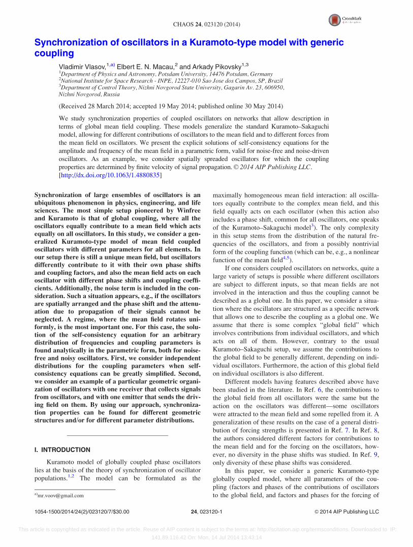
We consider a generic system of the Kuramoto-type
phase oscillators hi(t) having frequencies xi with the mean
field coupling depicted in Fig 1 Each oscillator j contributes
to the mean field H(t) with its own phase shift bj and cou-
pling constant Bj The mean field H(t) acts on oscillator iwith a specific phase shift ai and a coupling strength Ai
It is convenient to introduce additionally the overall
coupling strength e (eg by normalizing one or both of the
introduced quantities Ai Bj below for definiteness we
assume Ai Bjgt 0 because changing the sign of the coupling
can be absorbed to the phase shifts bj ai) and the overall
phase shift d (eg by normalizing the shifts bj ai)
Additionally we assume that the oscillators are subject to
independent Gaussian white noise forces (hniethtTHORNnjetht0THORNifrac14 2dijdetht t0THORN) with intensity D In this formulation the
equations of motions of the oscillators read
_hi frac14 xi thorn AieN
XN
jfrac141
Bj sinethhj bj hi thorn ai dTHORN thornffiffiffiffiDp
niethtTHORN
(1)
The system (1) can be rewritten in terms of the mean field
H(t)
_hi frac14 xi thorn Ai ImethHethtTHORNeiethhiaiTHORNTHORN thornffiffiffiffiDp
niethtTHORN
HethtTHORN frac14 eeid
N
XN
jfrac141
BjeiethhjbjTHORN (2)
It is convenient to reduce the number of parameters by a
transformation of phases ui frac14 hi ai Then the equations
for ui are
_ui frac14 xi thorn Ai Im HethtTHORNeiui
thorn
ffiffiffiffiDp
niethtTHORN
HethtTHORN frac14 eeid
N
XN
jfrac141
BjeiethujwjTHORN
(3)
where wjfrac14bj aj
This model appears to be the most generic one among
models of mean-field coupled Kuramoto-type phase oscilla-
tors If all the parameters of the coupling Ai Bi bi ai are
constant then the model reduces to the standard
KuramotondashSakaguchi one3 The case with different Ai ai
and xi of specific form has been considered previously in
Refs 9 and 11 Also the case with double delta distribution
of Ai has been studied in Ref 6 The case aifrac14bifrac14 0 was
considered in Ref 8 In Ref 10 the system (1) without noise
was examined Below we formulate the self-consistent equa-
tion for this model and present its explicit solution
It should be noted that the complex mean field H(t) is
different from the ldquoclassicalrdquo Kuramoto order parameter
N1P
j eiuj and can be larger than one depending on the pa-
rameters of the system Because this mean field yields the
forcing on the oscillators it serves as a natural order parame-
ter for this model
III SELF-CONSISTENCY CONDITION AND ITSSOLUTION
Here we formulate in the spirit of the original
Kuramoto approach a self-consistent equation for the mean
field H(t) in the thermodynamic limit and present its solution
In the thermodynamic limit the quantities x A B and whave a joint distribution density g(x)frac14 g(x A B w) where xis a general vector of parameters While formulating in a gen-
eral form we will consider below two specific situations (i)
all the quantities x A B and w are independent then g is a
product of four corresponding distribution densities and (ii)
situation where the coupling parameters A B and w are
determined by a geometrical position of an oscillator and thus
depend on this position parameterized by a scalar parameter
x while the frequency x is distributed independently of x
Introducing the conditional probability density function
qethu t j xTHORN we can rewrite the system (3) as
_u frac14 xthorn A Im HethtTHORNeiu
thornffiffiffiffiDp
nethtTHORNfrac14 xthorn A Q sinethH uTHORN thorn
ffiffiffiffiDp
nethtTHORN
HethtTHORN frac14 QeiH frac14 eeideth
gethxTHORNBeiweth2p
0
qethu t j xTHORNeiudu dx (4)
It is more convenient to write equations for Du frac14 uH
with the corresponding conditional probability density func-
tion qethDu t j xTHORN frac14 qethuH t j xTHORN
d
dtDu frac14 x _H A Q sinethDuTHORN thorn
ffiffiffiffiDp
nethtTHORN (5)
Q frac14 eeideth
gethxTHORNBeiweth2p
0
qethDu t j xTHORNeiDudDu dx (6)
The FokkerndashPlanck equation for the conditional probability
density function qethDu t j xTHORN follows from Eq (5)FIG 1 Configuration of the network coupled via the mean field H(t)
023120-2 Vlasov Macau and Pikovsky Chaos 24 023120 (2014)
This article is copyrighted as indicated in the article Reuse of AIP content is subject to the terms at httpscitationaiporgtermsconditions Downloaded to IP
1418911642 On Mon 14 Jul 2014 134314
qtthorn
Dux _H A Q sinethDuTHORN
q
frac14 D2qDu2
(7)
While one cannot a priori exclude complex regimes in
Eq (7) of particular importance are the simplest synchro-
nous states where the mean field H(t) rotates uniformly
(this corresponds to the classical Kuramoto solution)
Therefore we look for such solutions that the phase Hof the mean field H(t) rotates with a constant (yet
unknown) frequency X Correspondingly the distribution
of phase differences Du is stationary in the rotating with Xreference frame (such a solution is often called traveling
wave)
_H frac14 X _qethDu t j xTHORN frac14 0 (8)
Thus the equation for the stationary density qethDu t j xTHORNfrac14 qethDu j xTHORN reads
Dux X A Q sinethDuTHORNfrac12 qeth THORN frac14 D
2qDu2
(9)
Suppose we find solution of Eq (9) which then depends
on Q and X Denoting
FethXQTHORN frac14eth
gethxTHORNBeiweth2p
0
qethDu t j xTHORNeiDudDu dx (10)
we can then rewrite the self-consistency condition (6) as
Q frac14 eeidFethXQTHORN (11)
It is convenient to consider now Q X not as unknowns but
as parameters and to write explicit equations for the cou-
pling strength constants e d via these parameters
e frac14 Q
jFethXQTHORNj d frac14 argethFethXQTHORNTHORN (12)
This solution of the self-consistency problem is quite con-
venient for the numerical implementation as it reduces to
finding of solutions of the stationary FokkerndashPlanck equation
(9) and their integration (10) Below we consider separately
how this can be done in the noise-free case and in presence
of noise
IV NOISE-FREE CASE
In the case of vanishing noise Dfrac14 0 and Eq (9)
reduces to
Dux X A Q sinethDuTHORNfrac12 qeth THORN frac14 0 (13)
The solution of Eq (13) depends on the value of the parame-
ter A There are locked phases when jAj gt jX xj=Q so
x X A Q sinethDuTHORN frac14 0 and rotated phases when jAjlt jX xj=Q such that qfrac14CethAxTHORNjxXAQsinethDuTHORNj1
So the integral over parameter x in Eq (10) splits into two
integrals
FethXQTHORN frac14ethjAjgtjXxj=Q
gethxTHORNBeiw eiDuethAxTHORNdx
thornethjAjltjXxj=Q
gethxTHORNBeiw CethAxTHORN
eth2p
0
eiDu dDujx X A Q sinethDuTHORNj dx (14)
where in the first integral
sinethDuethAxTHORNTHORN frac14 X xA Q
and in the second one
CethAxTHORN frac14eth2p
0
dDujx X A Q sinethDuTHORNj
1
Integrations over Du in Eq (14) can be performed explicitly
CethAxTHORN frac14eth2p
0
dDujx X A QsinethDuTHORNj
1
frac14
ffiffiffiffiffiffiffiffiffiffiffiffiffiffiffiffiffiffiffiffiffiffiffiffiffiffiffiffiffiffiffiffiffiffiffiethX xTHORN2 A2Q2
q2p
eth2p
0
eiDu dDujx X A QsinethDuTHORNj frac14
2pi
AQ
X xjX xj
X xffiffiffiffiffiffiffiffiffiffiffiffiffiffiffiffiffiffiffiffiffiffiffiffiffiffiffiffiffiffiffiffiffiffiffiethX xTHORN2 A2Q2
q0
1A (15)
After substitution of Eq (15) into Eq (14) we obtain the final general expression for the main function F(X Q)
FethXQTHORN frac14ethjAjgtjXxj=Q
gethxTHORNBeiw
ffiffiffiffiffiffiffiffiffiffiffiffiffiffiffiffiffiffiffiffiffiffiffiffiffiffiffiffi1 ethX xTHORN2
A2Q2
sdx i
ethgethxTHORNBeiw X x
A Qdx
thorn i
ethjAjltjXxj=Q
gethxTHORNBeiw X xjX xj
ffiffiffiffiffiffiffiffiffiffiffiffiffiffiffiffiffiffiffiffiffiffiffiffiffiffiffiffiethX xTHORN2
A2Q2 1
sdx (16)
023120-3 Vlasov Macau and Pikovsky Chaos 24 023120 (2014)
This article is copyrighted as indicated in the article Reuse of AIP content is subject to the terms at httpscitationaiporgtermsconditions Downloaded to IP
1418911642 On Mon 14 Jul 2014 134314
A Independent parameters
The integrals in Eq (16) simplify in the case of inde-
pendent distributions of the parameters x A and B w That
means that gethxTHORN frac14 g1ethxATHORN g2ethBwTHORN In this case it is con-
venient to consider e and d as scaling parameters of the dis-
tribution ~g2eth ~B ~wTHORN such that
eeid frac14eth eth
~g2eth ~B ~wTHORN ~Bei~wd ~Bd~w (17)
so the parameters B frac14 ~B=e and w frac14 ~w d have such a dis-
tribution g2ethBwTHORN frac14 e~g2eth ~B ~wTHORN that satisfieseth ethg2ethBwTHORNBeiwdBdw frac14 1 (18)
From Eq (18) it follows that Eq (16) reduces because the
integration over B and w yields 1 to the following
expression
FethXQTHORN frac14eth ethjAjgtjXxj=Q
g1ethxATHORN
ffiffiffiffiffiffiffiffiffiffiffiffiffiffiffiffiffiffiffiffiffiffiffiffiffiffiffiffi1 ethX xTHORN2
A2Q2
sdAdx
i
eth ethg1ethxATHORN
X xA Q
dAdx
thorn i
eth ethjAjltjXxj=Q
g1ethxATHORN
X xjX xj
ffiffiffiffiffiffiffiffiffiffiffiffiffiffiffiffiffiffiffiffiffiffiffiffiffiffiffiffiethX xTHORN2
A2Q2 1
sdAdx (19)
Then the parameters e and d can be found from Eq (12)
depending on X and Q Noteworthy all the complexity of
distributions of parameters B and w is accumulated in values
of e and d while distributions of x A still contribute to the
integrals
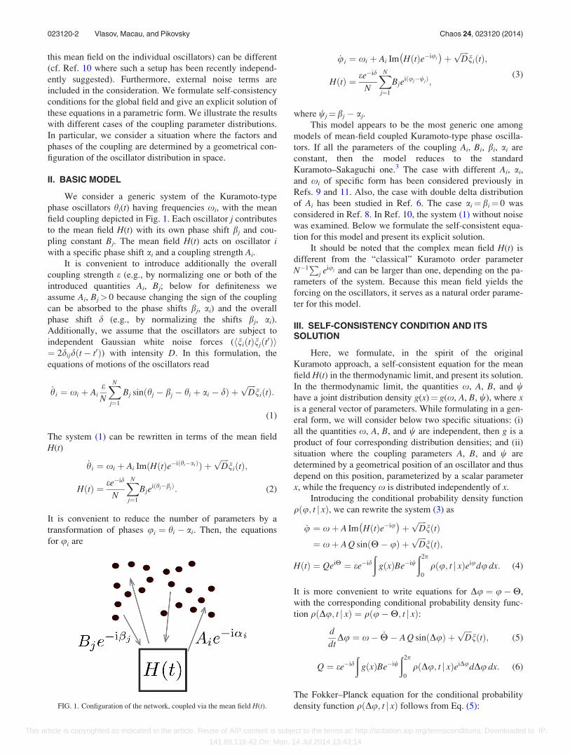
Below we give an example of application of our theory
In Fig 2 we present results of the calculation of the order
parameter Q and the frequency of the global field X as func-
tion e d for g1(x A)frac14 g(A)g(x) and gethATHORN frac14 Ah2 eA=h
gethxTHORN frac14 1ffiffiffiffi2pp ex2=2
Furthermore Eq (19) simplifies even more when the
individual frequencies of the oscillators are identical ie
when g(x)frac14 d(x x0) Then the integration over dx can
be performed first
FethXQTHORN frac14ethjAjgtjXx0j=Q
gethATHORN
ffiffiffiffiffiffiffiffiffiffiffiffiffiffiffiffiffiffiffiffiffiffiffiffiffiffiffiffiffiffi1 ethX x0THORN2
A2Q2
sdA
i
ethgethATHORNX x0
A QdA thorn i
ethjAjltjXx0j=Q
gethATHORN
X x0
jX x0j
ffiffiffiffiffiffiffiffiffiffiffiffiffiffiffiffiffiffiffiffiffiffiffiffiffiffiffiffiffiffiethX x0THORN2
A2Q2 1
sdA (20)
It is convenient to treat the function F(X Q) in Eq (20) as a
function of a new variable Y frac14 Xx0
Q which is a combination
of variables X and Q Then Eq (20) for F(X Q) transforms
to the following equation for F(Y)
FethYTHORN frac14ethjAjgtjYj
gethATHORNffiffiffiffiffiffiffiffiffiffiffiffiffiffi1 Y2
A2
rdA
i
ethgethATHORN Y
AdA thorn i
ethjAjltjYj
gethATHORN Y
jYj
ffiffiffiffiffiffiffiffiffiffiffiffiffiffiY2
A2 1
rdA (21)
where we took into account that Q 0
Despite the fact that Eq (12) are still valid for finding eand d it is more convenient to use Y and e as a parameters in
Eq (11) instead of Q and X Then the final expressions for
finding Q X and d take the following form
Q frac14 e jFethYTHORNj X frac14 x0 thorn eY jFethYTHORNj d frac14 argethFethYTHORNTHORN (22)
The results of the calculation of Q(e d) and X(e d) for
the identical natural frequencies are shown in Fig 3 where
we chose g1ethxATHORN frac14 Ah2 eA=hdethx x0THORN
Summarizing this section we have presented general
expressions for the order parameter frequency of the mean
field and the coupling parameters in a parametric form
These expressions are exemplified for specific distributions
of the strengths and phase shifts in the couplings in Figs 2
and 3 In the case of a distribution of natural frequencies
FIG 2 Dependencies of the amplitude Q of the mean field (a) and of its fre-
quency X on the parameters e and d for hfrac14 1 White area corresponds to
asynchronous state with vanishing mean field
023120-4 Vlasov Macau and Pikovsky Chaos 24 023120 (2014)
This article is copyrighted as indicated in the article Reuse of AIP content is subject to the terms at httpscitationaiporgtermsconditions Downloaded to IP
1418911642 On Mon 14 Jul 2014 134314
(Fig 2) there is a threshold in the coupling for the onset of
collective dynamics For the oscillators with equal frequen-
cies (Fig 3) there is no threshold
V SELF-CONSISTENT SOLUTION IN THE PRESENCEOF NOISE
Here we have to find the stationary solution of the
FokkerndashPlanck equation (9) It can be solved in the Fourier
modes representation
qethDu j xTHORN frac14 1
2p
Xn
CnethxTHORNeinDu
CnethxTHORN frac14eth2p
0
qeinDudDu C0ethxTHORN frac14 1 (23)
Substituting (23) in Eq (9) we obtain
eth2p
0
dDu
Duethfrac12xX AQ sinethDuTHORNqTHORN thornD
2qDu2
eikDu
frac14 k2DCk thorn ikethXxTHORNCk thorn ikAQCk1 Ckthorn1
2ifrac14 0 (24)
As a consequence we get a tridiagonal system of algebraic
equations
frac122kD i2ethX xTHORNCk thorn AQethCkthorn1 Ck1THORN frac14 0 (25)
The infinite system (25) can be solved by cutting it at some
large N as follows (see Ref 12)
Ck frac14 akCk1 ak frac14 2kD i2ethX xTHORN aN frac14AQ
aN
ak frac14AQ
ak thorn AQakthorn1
(26)
As a result C1 can be found recursively as a continued
fraction
C1 frac14 a1 frac14AQ
a1 thorn AQa2
frac14hellip (27)
From Eq (27) it is obvious that in general C1 is a function
of X Q x and A
C1 frac14 C1ethXQxATHORN (28)
The integral over Du in (10) can be calculated using the
Fourier-representation (23) yieldingeth2p
0
qethDu j xTHORNeiDudDu frac14 C1ethXQxATHORN (29)
Thus the expression for F in the case of noisy oscilla-
tors reads
FethXQTHORN frac14eth
gethxTHORNBeiwC1ethXQxATHORNdx (30)
A Independent parameters
From the expression (28) it follows that the integral in
Eq (30) simplifies in the same case of independent distribu-
tion of the parameters g(x)frac14 g1(x A) g2(B w) similar to the
noise-free case described in Sec IV Here we use the same
notations as before including condition (18)
The parameters e and d can be found from Eq (12)
where F(X Q) is determined from
FethXQTHORN frac14eth
g1ethxATHORNC1ethXQxATHORNdAdx (31)
In this way we obtain Q(e d) and X(e d) (Fig 4) For calcu-
lations we used the same distribution g1(x A) as in the
noise-free case
Contrary to the noise-free case when oscillatorrsquos indi-
vidual frequencies are identical (delta-function distribution)
no further simplification of F(X Q) appears possible In
Fig 5 we report the results for the same parameters as in
Fig 3 but with noise Dfrac14 1
In the considered model the main effect caused by noise
is the shift of the synchronization threshold to larger values
of the coupling strength e The noise acts very much similar
FIG 3 Dependencies of the amplitude Q of the mean field (a) and of its fre-
quency X on the parameters e and d for hfrac14 1 and x0frac14 0 White area corre-
sponds to asynchronous state with vanishing mean field
023120-5 Vlasov Macau and Pikovsky Chaos 24 023120 (2014)
This article is copyrighted as indicated in the article Reuse of AIP content is subject to the terms at httpscitationaiporgtermsconditions Downloaded to IP
1418911642 On Mon 14 Jul 2014 134314
to the distribution of natural frequencies if the oscillatorrsquos
individual frequencies are identical noise leads to a non-
zero threshold in the coupling
VI EXAMPLE OF A GEOMETRIC ORGANIZATION OFOSCILLATORS
In this section we present a particular example of appli-
cation of general expressions above to the case where distri-
butions of parameters are determined by configuration of
oscillators We consider spatially spreaded phase oscillators
with a common receiver that collects signals from all oscilla-
tors and with an emitter that receives the summarized signal
from the receiver and sends the coupling signal to the oscil-
lators below we assume that these signals propagate with
velocity c We assume that the oscillators have the same nat-
ural frequencies x0frac14 1 (cases where the frequencies are dis-
tributed (dependent or independent of geometric positions of
oscillators) can be straightforwardly treated within the same
framework)
We assume that oscillators are distributed uniformly on
a circle of radius r Each oscillator is thus labeled by the
angle xi (Fig 6) The receiver the emitter and the center of
the circle are supposed to lie on one line
Also we assume that the phase shifts bj and ai are pro-
portional to the distances between the oscillator the receiver
and the emitter so that the system can be described by
Eq (1) where
bj frac14x0
c
ffiffiffiffiffiffiffiffiffiffiffiffiffiffiffiffiffiffiffiffiffiffiffiffiffiffiffiffiffiffiffiffiffiffiffiffiffiffir2 thorn b2 2rb cos xj
q
ai frac14x0
c
ffiffiffiffiffiffiffiffiffiffiffiffiffiffiffiffiffiffiffiffiffiffiffiffiffiffiffiffiffiffiffiffiffiffiffiffiffiffir2 thorn a2 2ra cos xi
p (32)
Coupling strengths Bj and Ai are inversely proportional to the
square distances between each oscillator receiver and
emitter
FIG 4 The same as Fig 2 but with noise Dfrac14 1 FIG 5 The same as Fig 3 but with noise Dfrac14 1
FIG 6 Scheme of the system
023120-6 Vlasov Macau and Pikovsky Chaos 24 023120 (2014)
This article is copyrighted as indicated in the article Reuse of AIP content is subject to the terms at httpscitationaiporgtermsconditions Downloaded to IP
1418911642 On Mon 14 Jul 2014 134314
Bj frac141
r2 thorn b2 2rb cos xj Ai frac14
1
r2 thorn a2 2ra cos xi (33)
where a and b is the distances from the center of the circle
to the emitter and the receiver respectively (Fig 6) The
parameters e and d can be interpreted as a coupling coeffi-
cient and a phase shift for the signal transfer from the
receiver to the emitter
The theory developed above yields stable solutions for
any given parameters a and b Since all the oscillators have
the same natural frequencies the variable transformation
Yfrac14 (X x0)Q described in Sec III should be performed
Thus it is suitable to use Eq (22) in order to find Q X and
d as a functions of e and Y
In the numerical example presented in Fig 7 we fixed
bfrac14 r2 and varied a finding the order parameter Q(a) and
the frequency of the collective oscillations X(a) for efrac14 1 and
dfrac14 0 One can see a sequence of synchronization regions
separated by asynchronous intervals this is typical for sys-
tems with time delay in the couplingmdashin our case this delay
is due to separation of the emitter from the community of
oscillators and the finite speed of signal propagation
assumed The dependencies shown are not smooth because
as parameter a varies some oscillators enterleave the syn-
chronization domain
VII CONCLUSION
We have developed a theory of synchronization for
phase oscillators on networks with a special structure of cou-
pling through a global mean field A unified description of
the frequency and the amplitude of the mean field in a para-
metric form is valid both for noise-free and noisy oscillators
In the latter case numerical evaluation of a continued frac-
tion is needed otherwise the solution reduces to calculation
of integrals over parameter distributions As one of the
examples we considered a situation where contributions to
the mean field and its action on oscillators are prescribed by
a geometric configuration of the oscillators phase shifts and
the contribution factors result from the propagation of the
signals as waves having certain velocity The general formu-
lation we developed can be used for any such configuration
It appears that the method above may be useful also in more
general network setups where there is no global mean field
but such a field can be introduced as approximation (cf
Refs 13 and 14)
ACKNOWLEDGMENTS
VV thanks the IRTG 1740TRP 201150151-0 funded
by the DFGFAPESP
1Y Kuramoto Chemical Oscillations Waves and Turbulence (Springer
Berlin 1984)2J A Acebron L L Bonilla C J P Vicente F Ritort and R Spigler
Rev Mod Phys 77 137 (2005)3H Sakaguchi and Y Kuramoto Prog Theor Phys 76 576 (1986)4M Rosenblum and A Pikovsky Phys Rev Lett 98 064101 (2007)5A Pikovsky and M Rosenblum Physica D 238(1) 27 (2009)6H Hong and S H Strogatz Phys Rev Lett 106 054102 (2011)7D Iatsenko S Petkoski P V E McClintock and A Stefanovska Phys
Rev Lett 110 064101 (2013)8G H Paissan and D H Zanette Physica D 237 818 (2008)9E Montbrio and D Pazo Phys Rev Lett 106 254101 (2011)
10D Iatsenko P V E McClintock and A Stefanovska e-print arXiv13034453
[nlinAO]11E Montbrio and D Pazo Phys Rev E 84 046206 (2011) D Pazo and E
Montbrio Europhys Lett 95 60007 (2011)12H Z Risken The FokkerndashPlanck Equation (Springer Berlin 1989)13P S Skardal and J G Restrepo Phys Rev E 85 016208 (2012)14R Burioni M Casartelli M di Volo R Livi and A Vezzani e-print
arXiv13100985v2 [cond-matdis-nn]
FIG 7 The dependences of Q(a)
X(a) and Y(a) on the distance from the
center of the circle to the emitter a
bfrac14 05 rfrac14 1 efrac14 1 and dfrac14 0
Periodicity in a corresponds to the
zones of attractive and repulsive cou-
pling due to delay-induced phase shift
023120-7 Vlasov Macau and Pikovsky Chaos 24 023120 (2014)
This article is copyrighted as indicated in the article Reuse of AIP content is subject to the terms at httpscitationaiporgtermsconditions Downloaded to IP
1418911642 On Mon 14 Jul 2014 134314
this mean field on the individual oscillators) can be different
(cf Ref 10 where such a setup has been recently independ-
ently suggested) Furthermore external noise terms are
included in the consideration We formulate self-consistency
conditions for the global field and give an explicit solution of
these equations in a parametric form We illustrate the results
with different cases of the coupling parameter distributions
In particular we consider a situation where the factors and
phases of the coupling are determined by a geometrical con-
figuration of the oscillator distribution in space
II BASIC MODEL
We consider a generic system of the Kuramoto-type
phase oscillators hi(t) having frequencies xi with the mean
field coupling depicted in Fig 1 Each oscillator j contributes
to the mean field H(t) with its own phase shift bj and cou-
pling constant Bj The mean field H(t) acts on oscillator iwith a specific phase shift ai and a coupling strength Ai
It is convenient to introduce additionally the overall
coupling strength e (eg by normalizing one or both of the
introduced quantities Ai Bj below for definiteness we
assume Ai Bjgt 0 because changing the sign of the coupling
can be absorbed to the phase shifts bj ai) and the overall
phase shift d (eg by normalizing the shifts bj ai)
Additionally we assume that the oscillators are subject to
independent Gaussian white noise forces (hniethtTHORNnjetht0THORNifrac14 2dijdetht t0THORN) with intensity D In this formulation the
equations of motions of the oscillators read
_hi frac14 xi thorn AieN
XN
jfrac141
Bj sinethhj bj hi thorn ai dTHORN thornffiffiffiffiDp
niethtTHORN
(1)
The system (1) can be rewritten in terms of the mean field
H(t)
_hi frac14 xi thorn Ai ImethHethtTHORNeiethhiaiTHORNTHORN thornffiffiffiffiDp
niethtTHORN
HethtTHORN frac14 eeid
N
XN
jfrac141
BjeiethhjbjTHORN (2)
It is convenient to reduce the number of parameters by a
transformation of phases ui frac14 hi ai Then the equations
for ui are
_ui frac14 xi thorn Ai Im HethtTHORNeiui
thorn
ffiffiffiffiDp
niethtTHORN
HethtTHORN frac14 eeid
N
XN
jfrac141
BjeiethujwjTHORN
(3)
where wjfrac14bj aj
This model appears to be the most generic one among
models of mean-field coupled Kuramoto-type phase oscilla-
tors If all the parameters of the coupling Ai Bi bi ai are
constant then the model reduces to the standard
KuramotondashSakaguchi one3 The case with different Ai ai
and xi of specific form has been considered previously in
Refs 9 and 11 Also the case with double delta distribution
of Ai has been studied in Ref 6 The case aifrac14bifrac14 0 was
considered in Ref 8 In Ref 10 the system (1) without noise
was examined Below we formulate the self-consistent equa-
tion for this model and present its explicit solution
It should be noted that the complex mean field H(t) is
different from the ldquoclassicalrdquo Kuramoto order parameter
N1P
j eiuj and can be larger than one depending on the pa-
rameters of the system Because this mean field yields the
forcing on the oscillators it serves as a natural order parame-
ter for this model
III SELF-CONSISTENCY CONDITION AND ITSSOLUTION
Here we formulate in the spirit of the original
Kuramoto approach a self-consistent equation for the mean
field H(t) in the thermodynamic limit and present its solution
In the thermodynamic limit the quantities x A B and whave a joint distribution density g(x)frac14 g(x A B w) where xis a general vector of parameters While formulating in a gen-
eral form we will consider below two specific situations (i)
all the quantities x A B and w are independent then g is a
product of four corresponding distribution densities and (ii)
situation where the coupling parameters A B and w are
determined by a geometrical position of an oscillator and thus
depend on this position parameterized by a scalar parameter
x while the frequency x is distributed independently of x
Introducing the conditional probability density function
qethu t j xTHORN we can rewrite the system (3) as
_u frac14 xthorn A Im HethtTHORNeiu
thornffiffiffiffiDp
nethtTHORNfrac14 xthorn A Q sinethH uTHORN thorn
ffiffiffiffiDp
nethtTHORN
HethtTHORN frac14 QeiH frac14 eeideth
gethxTHORNBeiweth2p
0
qethu t j xTHORNeiudu dx (4)
It is more convenient to write equations for Du frac14 uH
with the corresponding conditional probability density func-
tion qethDu t j xTHORN frac14 qethuH t j xTHORN
d
dtDu frac14 x _H A Q sinethDuTHORN thorn
ffiffiffiffiDp
nethtTHORN (5)
Q frac14 eeideth
gethxTHORNBeiweth2p
0
qethDu t j xTHORNeiDudDu dx (6)
The FokkerndashPlanck equation for the conditional probability
density function qethDu t j xTHORN follows from Eq (5)FIG 1 Configuration of the network coupled via the mean field H(t)
023120-2 Vlasov Macau and Pikovsky Chaos 24 023120 (2014)
This article is copyrighted as indicated in the article Reuse of AIP content is subject to the terms at httpscitationaiporgtermsconditions Downloaded to IP
1418911642 On Mon 14 Jul 2014 134314
qtthorn
Dux _H A Q sinethDuTHORN
q
frac14 D2qDu2
(7)
While one cannot a priori exclude complex regimes in
Eq (7) of particular importance are the simplest synchro-
nous states where the mean field H(t) rotates uniformly
(this corresponds to the classical Kuramoto solution)
Therefore we look for such solutions that the phase Hof the mean field H(t) rotates with a constant (yet
unknown) frequency X Correspondingly the distribution
of phase differences Du is stationary in the rotating with Xreference frame (such a solution is often called traveling
wave)
_H frac14 X _qethDu t j xTHORN frac14 0 (8)
Thus the equation for the stationary density qethDu t j xTHORNfrac14 qethDu j xTHORN reads
Dux X A Q sinethDuTHORNfrac12 qeth THORN frac14 D
2qDu2
(9)
Suppose we find solution of Eq (9) which then depends
on Q and X Denoting
FethXQTHORN frac14eth
gethxTHORNBeiweth2p
0
qethDu t j xTHORNeiDudDu dx (10)
we can then rewrite the self-consistency condition (6) as
Q frac14 eeidFethXQTHORN (11)
It is convenient to consider now Q X not as unknowns but
as parameters and to write explicit equations for the cou-
pling strength constants e d via these parameters
e frac14 Q
jFethXQTHORNj d frac14 argethFethXQTHORNTHORN (12)
This solution of the self-consistency problem is quite con-
venient for the numerical implementation as it reduces to
finding of solutions of the stationary FokkerndashPlanck equation
(9) and their integration (10) Below we consider separately
how this can be done in the noise-free case and in presence
of noise
IV NOISE-FREE CASE
In the case of vanishing noise Dfrac14 0 and Eq (9)
reduces to
Dux X A Q sinethDuTHORNfrac12 qeth THORN frac14 0 (13)
The solution of Eq (13) depends on the value of the parame-
ter A There are locked phases when jAj gt jX xj=Q so
x X A Q sinethDuTHORN frac14 0 and rotated phases when jAjlt jX xj=Q such that qfrac14CethAxTHORNjxXAQsinethDuTHORNj1
So the integral over parameter x in Eq (10) splits into two
integrals
FethXQTHORN frac14ethjAjgtjXxj=Q
gethxTHORNBeiw eiDuethAxTHORNdx
thornethjAjltjXxj=Q
gethxTHORNBeiw CethAxTHORN
eth2p
0
eiDu dDujx X A Q sinethDuTHORNj dx (14)
where in the first integral
sinethDuethAxTHORNTHORN frac14 X xA Q
and in the second one
CethAxTHORN frac14eth2p
0
dDujx X A Q sinethDuTHORNj
1
Integrations over Du in Eq (14) can be performed explicitly
CethAxTHORN frac14eth2p
0
dDujx X A QsinethDuTHORNj
1
frac14
ffiffiffiffiffiffiffiffiffiffiffiffiffiffiffiffiffiffiffiffiffiffiffiffiffiffiffiffiffiffiffiffiffiffiffiethX xTHORN2 A2Q2
q2p
eth2p
0
eiDu dDujx X A QsinethDuTHORNj frac14
2pi
AQ
X xjX xj
X xffiffiffiffiffiffiffiffiffiffiffiffiffiffiffiffiffiffiffiffiffiffiffiffiffiffiffiffiffiffiffiffiffiffiffiethX xTHORN2 A2Q2
q0
1A (15)
After substitution of Eq (15) into Eq (14) we obtain the final general expression for the main function F(X Q)
FethXQTHORN frac14ethjAjgtjXxj=Q
gethxTHORNBeiw
ffiffiffiffiffiffiffiffiffiffiffiffiffiffiffiffiffiffiffiffiffiffiffiffiffiffiffiffi1 ethX xTHORN2
A2Q2
sdx i
ethgethxTHORNBeiw X x
A Qdx
thorn i
ethjAjltjXxj=Q
gethxTHORNBeiw X xjX xj
ffiffiffiffiffiffiffiffiffiffiffiffiffiffiffiffiffiffiffiffiffiffiffiffiffiffiffiffiethX xTHORN2
A2Q2 1
sdx (16)
023120-3 Vlasov Macau and Pikovsky Chaos 24 023120 (2014)
This article is copyrighted as indicated in the article Reuse of AIP content is subject to the terms at httpscitationaiporgtermsconditions Downloaded to IP
1418911642 On Mon 14 Jul 2014 134314
A Independent parameters
The integrals in Eq (16) simplify in the case of inde-
pendent distributions of the parameters x A and B w That
means that gethxTHORN frac14 g1ethxATHORN g2ethBwTHORN In this case it is con-
venient to consider e and d as scaling parameters of the dis-
tribution ~g2eth ~B ~wTHORN such that
eeid frac14eth eth
~g2eth ~B ~wTHORN ~Bei~wd ~Bd~w (17)
so the parameters B frac14 ~B=e and w frac14 ~w d have such a dis-
tribution g2ethBwTHORN frac14 e~g2eth ~B ~wTHORN that satisfieseth ethg2ethBwTHORNBeiwdBdw frac14 1 (18)
From Eq (18) it follows that Eq (16) reduces because the
integration over B and w yields 1 to the following
expression
FethXQTHORN frac14eth ethjAjgtjXxj=Q
g1ethxATHORN
ffiffiffiffiffiffiffiffiffiffiffiffiffiffiffiffiffiffiffiffiffiffiffiffiffiffiffiffi1 ethX xTHORN2
A2Q2
sdAdx
i
eth ethg1ethxATHORN
X xA Q
dAdx
thorn i
eth ethjAjltjXxj=Q
g1ethxATHORN
X xjX xj
ffiffiffiffiffiffiffiffiffiffiffiffiffiffiffiffiffiffiffiffiffiffiffiffiffiffiffiffiethX xTHORN2
A2Q2 1
sdAdx (19)
Then the parameters e and d can be found from Eq (12)
depending on X and Q Noteworthy all the complexity of
distributions of parameters B and w is accumulated in values
of e and d while distributions of x A still contribute to the
integrals
Below we give an example of application of our theory
In Fig 2 we present results of the calculation of the order
parameter Q and the frequency of the global field X as func-
tion e d for g1(x A)frac14 g(A)g(x) and gethATHORN frac14 Ah2 eA=h
gethxTHORN frac14 1ffiffiffiffi2pp ex2=2
Furthermore Eq (19) simplifies even more when the
individual frequencies of the oscillators are identical ie
when g(x)frac14 d(x x0) Then the integration over dx can
be performed first
FethXQTHORN frac14ethjAjgtjXx0j=Q
gethATHORN
ffiffiffiffiffiffiffiffiffiffiffiffiffiffiffiffiffiffiffiffiffiffiffiffiffiffiffiffiffiffi1 ethX x0THORN2
A2Q2
sdA
i
ethgethATHORNX x0
A QdA thorn i
ethjAjltjXx0j=Q
gethATHORN
X x0
jX x0j
ffiffiffiffiffiffiffiffiffiffiffiffiffiffiffiffiffiffiffiffiffiffiffiffiffiffiffiffiffiffiethX x0THORN2
A2Q2 1
sdA (20)
It is convenient to treat the function F(X Q) in Eq (20) as a
function of a new variable Y frac14 Xx0
Q which is a combination
of variables X and Q Then Eq (20) for F(X Q) transforms
to the following equation for F(Y)
FethYTHORN frac14ethjAjgtjYj
gethATHORNffiffiffiffiffiffiffiffiffiffiffiffiffiffi1 Y2
A2
rdA
i
ethgethATHORN Y
AdA thorn i
ethjAjltjYj
gethATHORN Y
jYj
ffiffiffiffiffiffiffiffiffiffiffiffiffiffiY2
A2 1
rdA (21)
where we took into account that Q 0
Despite the fact that Eq (12) are still valid for finding eand d it is more convenient to use Y and e as a parameters in
Eq (11) instead of Q and X Then the final expressions for
finding Q X and d take the following form
Q frac14 e jFethYTHORNj X frac14 x0 thorn eY jFethYTHORNj d frac14 argethFethYTHORNTHORN (22)
The results of the calculation of Q(e d) and X(e d) for
the identical natural frequencies are shown in Fig 3 where
we chose g1ethxATHORN frac14 Ah2 eA=hdethx x0THORN
Summarizing this section we have presented general
expressions for the order parameter frequency of the mean
field and the coupling parameters in a parametric form
These expressions are exemplified for specific distributions
of the strengths and phase shifts in the couplings in Figs 2
and 3 In the case of a distribution of natural frequencies
FIG 2 Dependencies of the amplitude Q of the mean field (a) and of its fre-
quency X on the parameters e and d for hfrac14 1 White area corresponds to
asynchronous state with vanishing mean field
023120-4 Vlasov Macau and Pikovsky Chaos 24 023120 (2014)
This article is copyrighted as indicated in the article Reuse of AIP content is subject to the terms at httpscitationaiporgtermsconditions Downloaded to IP
1418911642 On Mon 14 Jul 2014 134314
(Fig 2) there is a threshold in the coupling for the onset of
collective dynamics For the oscillators with equal frequen-
cies (Fig 3) there is no threshold
V SELF-CONSISTENT SOLUTION IN THE PRESENCEOF NOISE
Here we have to find the stationary solution of the
FokkerndashPlanck equation (9) It can be solved in the Fourier
modes representation
qethDu j xTHORN frac14 1
2p
Xn
CnethxTHORNeinDu
CnethxTHORN frac14eth2p
0
qeinDudDu C0ethxTHORN frac14 1 (23)
Substituting (23) in Eq (9) we obtain
eth2p
0
dDu
Duethfrac12xX AQ sinethDuTHORNqTHORN thornD
2qDu2
eikDu
frac14 k2DCk thorn ikethXxTHORNCk thorn ikAQCk1 Ckthorn1
2ifrac14 0 (24)
As a consequence we get a tridiagonal system of algebraic
equations
frac122kD i2ethX xTHORNCk thorn AQethCkthorn1 Ck1THORN frac14 0 (25)
The infinite system (25) can be solved by cutting it at some
large N as follows (see Ref 12)
Ck frac14 akCk1 ak frac14 2kD i2ethX xTHORN aN frac14AQ
aN
ak frac14AQ
ak thorn AQakthorn1
(26)
As a result C1 can be found recursively as a continued
fraction
C1 frac14 a1 frac14AQ
a1 thorn AQa2
frac14hellip (27)
From Eq (27) it is obvious that in general C1 is a function
of X Q x and A
C1 frac14 C1ethXQxATHORN (28)
The integral over Du in (10) can be calculated using the
Fourier-representation (23) yieldingeth2p
0
qethDu j xTHORNeiDudDu frac14 C1ethXQxATHORN (29)
Thus the expression for F in the case of noisy oscilla-
tors reads
FethXQTHORN frac14eth
gethxTHORNBeiwC1ethXQxATHORNdx (30)
A Independent parameters
From the expression (28) it follows that the integral in
Eq (30) simplifies in the same case of independent distribu-
tion of the parameters g(x)frac14 g1(x A) g2(B w) similar to the
noise-free case described in Sec IV Here we use the same
notations as before including condition (18)
The parameters e and d can be found from Eq (12)
where F(X Q) is determined from
FethXQTHORN frac14eth
g1ethxATHORNC1ethXQxATHORNdAdx (31)
In this way we obtain Q(e d) and X(e d) (Fig 4) For calcu-
lations we used the same distribution g1(x A) as in the
noise-free case
Contrary to the noise-free case when oscillatorrsquos indi-
vidual frequencies are identical (delta-function distribution)
no further simplification of F(X Q) appears possible In
Fig 5 we report the results for the same parameters as in
Fig 3 but with noise Dfrac14 1
In the considered model the main effect caused by noise
is the shift of the synchronization threshold to larger values
of the coupling strength e The noise acts very much similar
FIG 3 Dependencies of the amplitude Q of the mean field (a) and of its fre-
quency X on the parameters e and d for hfrac14 1 and x0frac14 0 White area corre-
sponds to asynchronous state with vanishing mean field
023120-5 Vlasov Macau and Pikovsky Chaos 24 023120 (2014)
This article is copyrighted as indicated in the article Reuse of AIP content is subject to the terms at httpscitationaiporgtermsconditions Downloaded to IP
1418911642 On Mon 14 Jul 2014 134314
to the distribution of natural frequencies if the oscillatorrsquos
individual frequencies are identical noise leads to a non-
zero threshold in the coupling
VI EXAMPLE OF A GEOMETRIC ORGANIZATION OFOSCILLATORS
In this section we present a particular example of appli-
cation of general expressions above to the case where distri-
butions of parameters are determined by configuration of
oscillators We consider spatially spreaded phase oscillators
with a common receiver that collects signals from all oscilla-
tors and with an emitter that receives the summarized signal
from the receiver and sends the coupling signal to the oscil-
lators below we assume that these signals propagate with
velocity c We assume that the oscillators have the same nat-
ural frequencies x0frac14 1 (cases where the frequencies are dis-
tributed (dependent or independent of geometric positions of
oscillators) can be straightforwardly treated within the same
framework)
We assume that oscillators are distributed uniformly on
a circle of radius r Each oscillator is thus labeled by the
angle xi (Fig 6) The receiver the emitter and the center of
the circle are supposed to lie on one line
Also we assume that the phase shifts bj and ai are pro-
portional to the distances between the oscillator the receiver
and the emitter so that the system can be described by
Eq (1) where
bj frac14x0
c
ffiffiffiffiffiffiffiffiffiffiffiffiffiffiffiffiffiffiffiffiffiffiffiffiffiffiffiffiffiffiffiffiffiffiffiffiffiffir2 thorn b2 2rb cos xj
q
ai frac14x0
c
ffiffiffiffiffiffiffiffiffiffiffiffiffiffiffiffiffiffiffiffiffiffiffiffiffiffiffiffiffiffiffiffiffiffiffiffiffiffir2 thorn a2 2ra cos xi
p (32)
Coupling strengths Bj and Ai are inversely proportional to the
square distances between each oscillator receiver and
emitter
FIG 4 The same as Fig 2 but with noise Dfrac14 1 FIG 5 The same as Fig 3 but with noise Dfrac14 1
FIG 6 Scheme of the system
023120-6 Vlasov Macau and Pikovsky Chaos 24 023120 (2014)
This article is copyrighted as indicated in the article Reuse of AIP content is subject to the terms at httpscitationaiporgtermsconditions Downloaded to IP
1418911642 On Mon 14 Jul 2014 134314
Bj frac141
r2 thorn b2 2rb cos xj Ai frac14
1
r2 thorn a2 2ra cos xi (33)
where a and b is the distances from the center of the circle
to the emitter and the receiver respectively (Fig 6) The
parameters e and d can be interpreted as a coupling coeffi-
cient and a phase shift for the signal transfer from the
receiver to the emitter
The theory developed above yields stable solutions for
any given parameters a and b Since all the oscillators have
the same natural frequencies the variable transformation
Yfrac14 (X x0)Q described in Sec III should be performed
Thus it is suitable to use Eq (22) in order to find Q X and
d as a functions of e and Y
In the numerical example presented in Fig 7 we fixed
bfrac14 r2 and varied a finding the order parameter Q(a) and
the frequency of the collective oscillations X(a) for efrac14 1 and
dfrac14 0 One can see a sequence of synchronization regions
separated by asynchronous intervals this is typical for sys-
tems with time delay in the couplingmdashin our case this delay
is due to separation of the emitter from the community of
oscillators and the finite speed of signal propagation
assumed The dependencies shown are not smooth because
as parameter a varies some oscillators enterleave the syn-
chronization domain
VII CONCLUSION
We have developed a theory of synchronization for
phase oscillators on networks with a special structure of cou-
pling through a global mean field A unified description of
the frequency and the amplitude of the mean field in a para-
metric form is valid both for noise-free and noisy oscillators
In the latter case numerical evaluation of a continued frac-
tion is needed otherwise the solution reduces to calculation
of integrals over parameter distributions As one of the
examples we considered a situation where contributions to
the mean field and its action on oscillators are prescribed by
a geometric configuration of the oscillators phase shifts and
the contribution factors result from the propagation of the
signals as waves having certain velocity The general formu-
lation we developed can be used for any such configuration
It appears that the method above may be useful also in more
general network setups where there is no global mean field
but such a field can be introduced as approximation (cf
Refs 13 and 14)
ACKNOWLEDGMENTS
VV thanks the IRTG 1740TRP 201150151-0 funded
by the DFGFAPESP
1Y Kuramoto Chemical Oscillations Waves and Turbulence (Springer
Berlin 1984)2J A Acebron L L Bonilla C J P Vicente F Ritort and R Spigler
Rev Mod Phys 77 137 (2005)3H Sakaguchi and Y Kuramoto Prog Theor Phys 76 576 (1986)4M Rosenblum and A Pikovsky Phys Rev Lett 98 064101 (2007)5A Pikovsky and M Rosenblum Physica D 238(1) 27 (2009)6H Hong and S H Strogatz Phys Rev Lett 106 054102 (2011)7D Iatsenko S Petkoski P V E McClintock and A Stefanovska Phys
Rev Lett 110 064101 (2013)8G H Paissan and D H Zanette Physica D 237 818 (2008)9E Montbrio and D Pazo Phys Rev Lett 106 254101 (2011)
10D Iatsenko P V E McClintock and A Stefanovska e-print arXiv13034453
[nlinAO]11E Montbrio and D Pazo Phys Rev E 84 046206 (2011) D Pazo and E
Montbrio Europhys Lett 95 60007 (2011)12H Z Risken The FokkerndashPlanck Equation (Springer Berlin 1989)13P S Skardal and J G Restrepo Phys Rev E 85 016208 (2012)14R Burioni M Casartelli M di Volo R Livi and A Vezzani e-print
arXiv13100985v2 [cond-matdis-nn]
FIG 7 The dependences of Q(a)
X(a) and Y(a) on the distance from the
center of the circle to the emitter a
bfrac14 05 rfrac14 1 efrac14 1 and dfrac14 0
Periodicity in a corresponds to the
zones of attractive and repulsive cou-
pling due to delay-induced phase shift
023120-7 Vlasov Macau and Pikovsky Chaos 24 023120 (2014)
This article is copyrighted as indicated in the article Reuse of AIP content is subject to the terms at httpscitationaiporgtermsconditions Downloaded to IP
1418911642 On Mon 14 Jul 2014 134314
A Independent parameters
The integrals in Eq (16) simplify in the case of inde-
pendent distributions of the parameters x A and B w That
means that gethxTHORN frac14 g1ethxATHORN g2ethBwTHORN In this case it is con-
venient to consider e and d as scaling parameters of the dis-
tribution ~g2eth ~B ~wTHORN such that
eeid frac14eth eth
~g2eth ~B ~wTHORN ~Bei~wd ~Bd~w (17)
so the parameters B frac14 ~B=e and w frac14 ~w d have such a dis-
tribution g2ethBwTHORN frac14 e~g2eth ~B ~wTHORN that satisfieseth ethg2ethBwTHORNBeiwdBdw frac14 1 (18)
From Eq (18) it follows that Eq (16) reduces because the
integration over B and w yields 1 to the following
expression
FethXQTHORN frac14eth ethjAjgtjXxj=Q
g1ethxATHORN
ffiffiffiffiffiffiffiffiffiffiffiffiffiffiffiffiffiffiffiffiffiffiffiffiffiffiffiffi1 ethX xTHORN2
A2Q2
sdAdx
i
eth ethg1ethxATHORN
X xA Q
dAdx
thorn i
eth ethjAjltjXxj=Q
g1ethxATHORN
X xjX xj
ffiffiffiffiffiffiffiffiffiffiffiffiffiffiffiffiffiffiffiffiffiffiffiffiffiffiffiffiethX xTHORN2
A2Q2 1
sdAdx (19)
Then the parameters e and d can be found from Eq (12)
depending on X and Q Noteworthy all the complexity of
distributions of parameters B and w is accumulated in values
of e and d while distributions of x A still contribute to the
integrals
Below we give an example of application of our theory
In Fig 2 we present results of the calculation of the order
parameter Q and the frequency of the global field X as func-
tion e d for g1(x A)frac14 g(A)g(x) and gethATHORN frac14 Ah2 eA=h
gethxTHORN frac14 1ffiffiffiffi2pp ex2=2
Furthermore Eq (19) simplifies even more when the
individual frequencies of the oscillators are identical ie
when g(x)frac14 d(x x0) Then the integration over dx can
be performed first
FethXQTHORN frac14ethjAjgtjXx0j=Q
gethATHORN
ffiffiffiffiffiffiffiffiffiffiffiffiffiffiffiffiffiffiffiffiffiffiffiffiffiffiffiffiffiffi1 ethX x0THORN2
A2Q2
sdA
i
ethgethATHORNX x0
A QdA thorn i
ethjAjltjXx0j=Q
gethATHORN
X x0
jX x0j
ffiffiffiffiffiffiffiffiffiffiffiffiffiffiffiffiffiffiffiffiffiffiffiffiffiffiffiffiffiffiethX x0THORN2
A2Q2 1
sdA (20)
It is convenient to treat the function F(X Q) in Eq (20) as a
function of a new variable Y frac14 Xx0
Q which is a combination
of variables X and Q Then Eq (20) for F(X Q) transforms
to the following equation for F(Y)
FethYTHORN frac14ethjAjgtjYj
gethATHORNffiffiffiffiffiffiffiffiffiffiffiffiffiffi1 Y2
A2
rdA
i
ethgethATHORN Y
AdA thorn i
ethjAjltjYj
gethATHORN Y
jYj
ffiffiffiffiffiffiffiffiffiffiffiffiffiffiY2
A2 1
rdA (21)
where we took into account that Q 0
Despite the fact that Eq (12) are still valid for finding eand d it is more convenient to use Y and e as a parameters in
Eq (11) instead of Q and X Then the final expressions for
finding Q X and d take the following form
Q frac14 e jFethYTHORNj X frac14 x0 thorn eY jFethYTHORNj d frac14 argethFethYTHORNTHORN (22)
The results of the calculation of Q(e d) and X(e d) for
the identical natural frequencies are shown in Fig 3 where
we chose g1ethxATHORN frac14 Ah2 eA=hdethx x0THORN
Summarizing this section we have presented general
expressions for the order parameter frequency of the mean
field and the coupling parameters in a parametric form
These expressions are exemplified for specific distributions
of the strengths and phase shifts in the couplings in Figs 2
and 3 In the case of a distribution of natural frequencies
FIG 2 Dependencies of the amplitude Q of the mean field (a) and of its fre-
quency X on the parameters e and d for hfrac14 1 White area corresponds to
asynchronous state with vanishing mean field
023120-4 Vlasov Macau and Pikovsky Chaos 24 023120 (2014)
This article is copyrighted as indicated in the article Reuse of AIP content is subject to the terms at httpscitationaiporgtermsconditions Downloaded to IP
1418911642 On Mon 14 Jul 2014 134314
(Fig 2) there is a threshold in the coupling for the onset of
collective dynamics For the oscillators with equal frequen-
cies (Fig 3) there is no threshold
V SELF-CONSISTENT SOLUTION IN THE PRESENCEOF NOISE
Here we have to find the stationary solution of the
FokkerndashPlanck equation (9) It can be solved in the Fourier
modes representation
qethDu j xTHORN frac14 1
2p
Xn
CnethxTHORNeinDu
CnethxTHORN frac14eth2p
0
qeinDudDu C0ethxTHORN frac14 1 (23)
Substituting (23) in Eq (9) we obtain
eth2p
0
dDu
Duethfrac12xX AQ sinethDuTHORNqTHORN thornD
2qDu2
eikDu
frac14 k2DCk thorn ikethXxTHORNCk thorn ikAQCk1 Ckthorn1
2ifrac14 0 (24)
As a consequence we get a tridiagonal system of algebraic
equations
frac122kD i2ethX xTHORNCk thorn AQethCkthorn1 Ck1THORN frac14 0 (25)
The infinite system (25) can be solved by cutting it at some
large N as follows (see Ref 12)
Ck frac14 akCk1 ak frac14 2kD i2ethX xTHORN aN frac14AQ
aN
ak frac14AQ
ak thorn AQakthorn1
(26)
As a result C1 can be found recursively as a continued
fraction
C1 frac14 a1 frac14AQ
a1 thorn AQa2
frac14hellip (27)
From Eq (27) it is obvious that in general C1 is a function
of X Q x and A
C1 frac14 C1ethXQxATHORN (28)
The integral over Du in (10) can be calculated using the
Fourier-representation (23) yieldingeth2p
0
qethDu j xTHORNeiDudDu frac14 C1ethXQxATHORN (29)
Thus the expression for F in the case of noisy oscilla-
tors reads
FethXQTHORN frac14eth
gethxTHORNBeiwC1ethXQxATHORNdx (30)
A Independent parameters
From the expression (28) it follows that the integral in
Eq (30) simplifies in the same case of independent distribu-
tion of the parameters g(x)frac14 g1(x A) g2(B w) similar to the
noise-free case described in Sec IV Here we use the same
notations as before including condition (18)
The parameters e and d can be found from Eq (12)
where F(X Q) is determined from
FethXQTHORN frac14eth
g1ethxATHORNC1ethXQxATHORNdAdx (31)
In this way we obtain Q(e d) and X(e d) (Fig 4) For calcu-
lations we used the same distribution g1(x A) as in the
noise-free case
Contrary to the noise-free case when oscillatorrsquos indi-
vidual frequencies are identical (delta-function distribution)
no further simplification of F(X Q) appears possible In
Fig 5 we report the results for the same parameters as in
Fig 3 but with noise Dfrac14 1
In the considered model the main effect caused by noise
is the shift of the synchronization threshold to larger values
of the coupling strength e The noise acts very much similar
FIG 3 Dependencies of the amplitude Q of the mean field (a) and of its fre-
quency X on the parameters e and d for hfrac14 1 and x0frac14 0 White area corre-
sponds to asynchronous state with vanishing mean field
023120-5 Vlasov Macau and Pikovsky Chaos 24 023120 (2014)
This article is copyrighted as indicated in the article Reuse of AIP content is subject to the terms at httpscitationaiporgtermsconditions Downloaded to IP
1418911642 On Mon 14 Jul 2014 134314
to the distribution of natural frequencies if the oscillatorrsquos
individual frequencies are identical noise leads to a non-
zero threshold in the coupling
VI EXAMPLE OF A GEOMETRIC ORGANIZATION OFOSCILLATORS
In this section we present a particular example of appli-
cation of general expressions above to the case where distri-
butions of parameters are determined by configuration of
oscillators We consider spatially spreaded phase oscillators
with a common receiver that collects signals from all oscilla-
tors and with an emitter that receives the summarized signal
from the receiver and sends the coupling signal to the oscil-
lators below we assume that these signals propagate with
velocity c We assume that the oscillators have the same nat-
ural frequencies x0frac14 1 (cases where the frequencies are dis-
tributed (dependent or independent of geometric positions of
oscillators) can be straightforwardly treated within the same
framework)
We assume that oscillators are distributed uniformly on
a circle of radius r Each oscillator is thus labeled by the
angle xi (Fig 6) The receiver the emitter and the center of
the circle are supposed to lie on one line
Also we assume that the phase shifts bj and ai are pro-
portional to the distances between the oscillator the receiver
and the emitter so that the system can be described by
Eq (1) where
bj frac14x0
c
ffiffiffiffiffiffiffiffiffiffiffiffiffiffiffiffiffiffiffiffiffiffiffiffiffiffiffiffiffiffiffiffiffiffiffiffiffiffir2 thorn b2 2rb cos xj
q
ai frac14x0
c
ffiffiffiffiffiffiffiffiffiffiffiffiffiffiffiffiffiffiffiffiffiffiffiffiffiffiffiffiffiffiffiffiffiffiffiffiffiffir2 thorn a2 2ra cos xi
p (32)
Coupling strengths Bj and Ai are inversely proportional to the
square distances between each oscillator receiver and
emitter
FIG 4 The same as Fig 2 but with noise Dfrac14 1 FIG 5 The same as Fig 3 but with noise Dfrac14 1
FIG 6 Scheme of the system
023120-6 Vlasov Macau and Pikovsky Chaos 24 023120 (2014)
This article is copyrighted as indicated in the article Reuse of AIP content is subject to the terms at httpscitationaiporgtermsconditions Downloaded to IP
1418911642 On Mon 14 Jul 2014 134314
Bj frac141
r2 thorn b2 2rb cos xj Ai frac14
1
r2 thorn a2 2ra cos xi (33)
where a and b is the distances from the center of the circle
to the emitter and the receiver respectively (Fig 6) The
parameters e and d can be interpreted as a coupling coeffi-
cient and a phase shift for the signal transfer from the
receiver to the emitter
The theory developed above yields stable solutions for
any given parameters a and b Since all the oscillators have
the same natural frequencies the variable transformation
Yfrac14 (X x0)Q described in Sec III should be performed
Thus it is suitable to use Eq (22) in order to find Q X and
d as a functions of e and Y
In the numerical example presented in Fig 7 we fixed
bfrac14 r2 and varied a finding the order parameter Q(a) and
the frequency of the collective oscillations X(a) for efrac14 1 and
dfrac14 0 One can see a sequence of synchronization regions
separated by asynchronous intervals this is typical for sys-
tems with time delay in the couplingmdashin our case this delay
is due to separation of the emitter from the community of
oscillators and the finite speed of signal propagation
assumed The dependencies shown are not smooth because
as parameter a varies some oscillators enterleave the syn-
chronization domain
VII CONCLUSION
We have developed a theory of synchronization for
phase oscillators on networks with a special structure of cou-
pling through a global mean field A unified description of
the frequency and the amplitude of the mean field in a para-
metric form is valid both for noise-free and noisy oscillators
In the latter case numerical evaluation of a continued frac-
tion is needed otherwise the solution reduces to calculation
of integrals over parameter distributions As one of the
examples we considered a situation where contributions to
the mean field and its action on oscillators are prescribed by
a geometric configuration of the oscillators phase shifts and
the contribution factors result from the propagation of the
signals as waves having certain velocity The general formu-
lation we developed can be used for any such configuration
It appears that the method above may be useful also in more
general network setups where there is no global mean field
but such a field can be introduced as approximation (cf
Refs 13 and 14)
ACKNOWLEDGMENTS
VV thanks the IRTG 1740TRP 201150151-0 funded
by the DFGFAPESP
1Y Kuramoto Chemical Oscillations Waves and Turbulence (Springer
Berlin 1984)2J A Acebron L L Bonilla C J P Vicente F Ritort and R Spigler
Rev Mod Phys 77 137 (2005)3H Sakaguchi and Y Kuramoto Prog Theor Phys 76 576 (1986)4M Rosenblum and A Pikovsky Phys Rev Lett 98 064101 (2007)5A Pikovsky and M Rosenblum Physica D 238(1) 27 (2009)6H Hong and S H Strogatz Phys Rev Lett 106 054102 (2011)7D Iatsenko S Petkoski P V E McClintock and A Stefanovska Phys
Rev Lett 110 064101 (2013)8G H Paissan and D H Zanette Physica D 237 818 (2008)9E Montbrio and D Pazo Phys Rev Lett 106 254101 (2011)
10D Iatsenko P V E McClintock and A Stefanovska e-print arXiv13034453
[nlinAO]11E Montbrio and D Pazo Phys Rev E 84 046206 (2011) D Pazo and E
Montbrio Europhys Lett 95 60007 (2011)12H Z Risken The FokkerndashPlanck Equation (Springer Berlin 1989)13P S Skardal and J G Restrepo Phys Rev E 85 016208 (2012)14R Burioni M Casartelli M di Volo R Livi and A Vezzani e-print
arXiv13100985v2 [cond-matdis-nn]
FIG 7 The dependences of Q(a)
X(a) and Y(a) on the distance from the
center of the circle to the emitter a
bfrac14 05 rfrac14 1 efrac14 1 and dfrac14 0
Periodicity in a corresponds to the
zones of attractive and repulsive cou-
pling due to delay-induced phase shift
023120-7 Vlasov Macau and Pikovsky Chaos 24 023120 (2014)
This article is copyrighted as indicated in the article Reuse of AIP content is subject to the terms at httpscitationaiporgtermsconditions Downloaded to IP
1418911642 On Mon 14 Jul 2014 134314
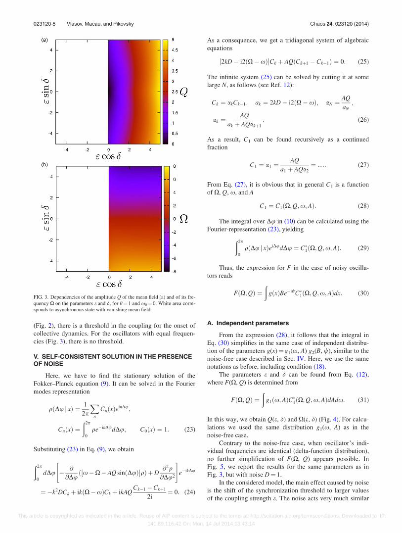
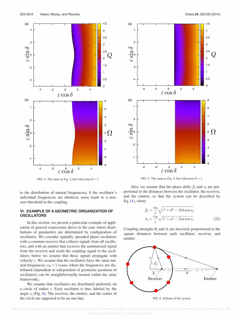
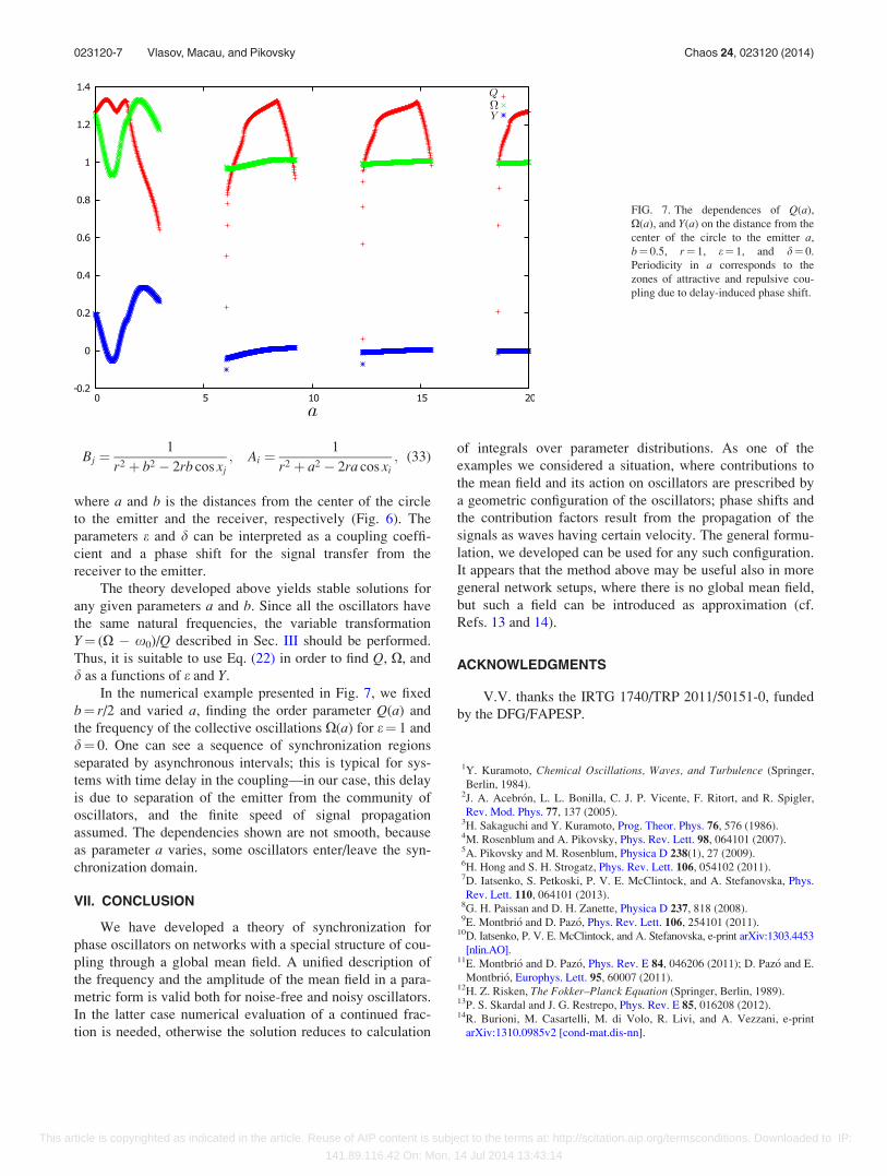