synchrophasor applications for wind power generation · mpp maximum power point . mppt maximum...

NREL is a national laboratory of the U.S. Department of Energy Office of Energy Efficiency & Renewable Energy Operated by the Alliance for Sustainable Energy, LLC

This report is available at no cost from the National Renewable Energy Laboratory (NREL) at www.nrel.gov/publications.

Contract No. DE-AC36-08GO28308

Synchrophasor Applications for Wind Power Generation E. Muljadi, Y.C. Zhang, A. Allen, M. Singh, V. Gevorgian, and Y.-H. Wan National Renewable Energy Laboratory

Technical Report NREL/TP-5D00-60772 February 2014

NREL is a national laboratory of the U.S. Department of Energy Office of Energy Efficiency & Renewable Energy Operated by the Alliance for Sustainable Energy, LLC


Contract No. DE-AC36-08GO28308

National Renewable Energy Laboratory 15013 Denver West Parkway Golden, CO 80401 303-275-3000 • www.nrel.gov

Synchrophasor Applications for Wind Power Generation E. Muljadi, Y.C. Zhang, A. Allen, M. Singh, and V. Gevorgian National Renewable Energy Laboratory

Prepared under Task No. WE11.0930

Technical Report NREL/TP-5D00-60772 February 2014

NOTICE

This report was prepared as an account of work sponsored by an agency of the United States government. Neither the United States government nor any agency thereof, nor any of their employees, makes any warranty, express or implied, or assumes any legal liability or responsibility for the accuracy, completeness, or usefulness of any information, apparatus, product, or process disclosed, or represents that its use would not infringe privately owned rights. Reference herein to any specific commercial product, process, or service by trade name, trademark, manufacturer, or otherwise does not necessarily constitute or imply its endorsement, recommendation, or favoring by the United States government or any agency thereof. The views and opinions of authors expressed herein do not necessarily state or reflect those of the United States government or any agency thereof.


Available electronically at http://www.osti.gov/bridge

Available for a processing fee to U.S. Department of Energy and its contractors, in paper, from:

U.S. Department of Energy Office of Scientific and Technical Information P.O. Box 62 Oak Ridge, TN 37831-0062 phone: 865.576.8401 fax: 865.576.5728 email: mailto:[email protected]

Available for sale to the public, in paper, from:

U.S. Department of Commerce National Technical Information Service 5285 Port Royal Road Springfield, VA 22161 phone: 800.553.6847 fax: 703.605.6900 email: [email protected] online ordering: http://www.ntis.gov/help/ordermethods.aspx

Cover Photos: (left to right) photo by Pat Corkery, NREL 16416, photo from SunEdison, NREL 17423, photo by Pat Corkery, NREL 16560, photo by Dennis Schroeder, NREL 17613, photo by Dean Armstrong, NREL 17436, photo by Pat Corkery, NREL 17721.

Printed on paper containing at least 50% wastepaper, including 10% post consumer waste.

http://www.osti.gov/bridge

mailto:[email protected]

mailto:[email protected]

http://www.ntis.gov/help/ordermethods.aspx

iii


List of Acronyms 3LG three-lines-to-ground AC alternating current CPP conventional power plant CR-CSI current-regulated current source inverter CR-VSI current-regulated voltage source inverter CSD cross-spectral density DC direct current DFIG doubly-fed induction generator DOE U.S. Department of Energy ERCOT Electric Reliability Council of Texas GPS Global Positioning System IEEE Institute of Electrical and Electronics Engineers IGBT insulated-gate bipolar transistor LL line-to-line LLG line-to-line-to-ground MPP maximum power point MPPT Maximum Power Point Tracking NREL National Renewable Energy Laboratory PLL phase-locked loop PMU phasor measurement unit PSD power spectral density PSLF Positive Sequence Load Flow PV photovoltaic PVP photovoltaic power plants PWM pulse-width modulation RMS root mean square SCC short-circuit current SCE Southern California Edison SLG single-line-to-ground WECC Western Electricity Coordinating Council WPP wind power plant

iv


Executive Summary The U.S. power industry is undertaking several initiatives that will improve the operations of the electric power grid. One of those is the implementation of wide-area measurements using phasor measurement units to dynamically monitor the operations and status of the network and provide advanced situational awareness and stability assessment.

This report is intended to present the potential future applications of synchrophasors for power system operations under high penetrations of wind and other renewable energy sources. Brief overviews of synchrophasors and stability analysis are presented. Several sections were developed based on previous work related to the synchrophasor subtask, and one section was developed to capture the wider spectrum on power system stability, which will benefit from synchrophasor-related work. One section is dedicated to the investigative methods in estimating wind power plant inertia using synchrophasor data, and another section focuses on the effects of wind power plant integration and the resulting displacement of conventional power plant inertia on inter- and intra-area modes using synchrophasor measurement–based (without the knowledge of the power system network) data.

The potential utilization of synchrophasors in modern power systems is very broad. This report covers only a small portion of the potential applications in wind power generation.

v


Table of Contents 1 Introduction ........................................................................................................................................... 1

1.1 Synchrophasors—PMUs .................................................................................................................. 1 1.2 Summary .......................................................................................................................................... 5 1.3 References ........................................................................................................................................ 5

2 WPP Stability Evaluation ..................................................................................................................... 6 2.1 Background ...................................................................................................................................... 6 2.2 Rotor-Angle Stability ....................................................................................................................... 6

2.2.1 Loss of Line ...................................................................................................................... 7 2.2.2 Self-Clearing Faults ........................................................................................................ 10 2.2.3 Line Opened to Clear the Fault ....................................................................................... 15 2.2.4 Example Using the WECC Network............................................................................... 17 2.2.5 Example Using a WPP in the WECC Network .............................................................. 20 2.2.6 Example Using a WPP in the WECC Network .............................................................. 21

2.3 Voltage Stability ............................................................................................................................ 23 2.3.1 Parallel Compensation .................................................................................................... 24 2.3.2 Series Compensation ....................................................................................................... 25 2.3.3 PV and VQ Curves .......................................................................................................... 26 2.3.4 PMU-Enhanced Dynamic Stability Assessment ............................................................. 29 2.3.5 Impact on the Voltage Magnitude ................................................................................... 30 2.3.6 Impact on the Voltage Angle (δ) ..................................................................................... 32

2.4 Frequency Stability ........................................................................................................................ 35 2.5 Summary ........................................................................................................................................ 35 2.6 References ...................................................................................................................................... 36

3 PMU–Based Wind Plant Equivalent Inertia Assessment ................................................................ 38 3.1 Background .................................................................................................................................... 38 3.2 Mathematical Methods................................................................................................................... 39 3.3 Case Studies ................................................................................................................................... 42

3.3.1 Two-Machine Infinite-Bus System ................................................................................. 42 3.3.2 Interconnection-Wide System ......................................................................................... 44 3.3.3 PMU Data Testing .......................................................................................................... 47

3.4 Summary ........................................................................................................................................ 49 3.5 References ...................................................................................................................................... 49

4 Measurement-Based Investigation of Inter- and Intra-Area Power System Stability for WPP Integration ........................................................................................................................................... 51 4.1 Background .................................................................................................................................... 51 4.2 Model Development....................................................................................................................... 52

4.2.1 Two-Area System Model ................................................................................................ 52 4.2.2 WPP Model ..................................................................................................................... 53 4.2.3 Additional WPP Controls ................................................................................................ 54

4.3 Simulated Phasor Data Processing ................................................................................................. 54 4.4 Simulation Cases ............................................................................................................................ 55

4.4.1 Additional WPP Controls ................................................................................................ 57 4.5 Results and Discussions ................................................................................................................. 57

4.5.1 PSD Analysis .................................................................................................................. 57 4.5.2 CSD Analysis .................................................................................................................. 59 4.5.3 Matrix-Pencil Analysis Technique .................................................................................. 61 4.5.4 Modes with Additional WPP Controls ............................................................................ 62

4.6 Summary ........................................................................................................................................ 64 4.7 References ...................................................................................................................................... 64

vi


List of Figures Figure 1. A typical sinusoidal waveform of an AC voltage ..................................................................... 2 Figure 2. Example of a Phasor File graphic display ................................................................................ 3 Figure 3. Power system stability classification [1] .................................................................................. 6 Figure 4. A simple two-bus system illustrating rotor-angle dynamic stability [2–3] ........................... 7 Figure 5. Voltage and power angle δ illustrating the dynamic when one line is out of service .......... 8 Figure 6. Voltage phasors for two differently-sized line impedances ................................................... 9 Figure 7. Dynamic behavior of real and reactive power during one line removal................................ 9 Figure 8. Voltage and power angles of an unstable post-transient illustrating the removal of

two of the three parallel lines ............................................................................................................ 10 Figure 9. Voltage, real, and reactive power computed by the power flow program (PSLF) .............. 11 Figure 10. Steady-state angle stability assessment—stable operation .............................................. 12 Figure 11. Self-clearing fault for a duration of nine cycles ................................................................... 13 Figure 12. Steady-state angle stability assessment—unbstable operation ........................................ 14 Figure 13. Voltage magnitude and corresponding angle (stability limit) of the self-clearing

fault at the critical clearing time ........................................................................................................ 14 Figure 14. A single-line diagram illustrating a line opening to clear a fault ....................................... 15 Figure 15. Steady-state angle stability assessment (line opened to clear a fault) during the

critical clearing time ........................................................................................................................... 15 Figure 16. Fault clearing by opening the line (∆tCR = 12.6 cycles) ....................................................... 16 Figure 17. Phasor diagram of a single generator connected to an infinite bus and a large

multi-bus system ................................................................................................................................ 17 Figure 18. The LVRT requirement per the Large Generator Interconnection Agreement in

Appendix G of the Federal Energy Regulatory Commission’s Order 661 .................................... 18 Figure 19. Voltage and frequency at the point of interconnection and the LVRT drawn on

the same figure ................................................................................................................................... 18 Figure 20. Voltage and angle at the generator ....................................................................................... 19 Figure 21. Real power and reactive power dynamic ............................................................................. 19 Figure 22. Single-line diagram of a WPP and nearby buses ................................................................ 21 Figure 23. The voltage and angle at the wind turbine generator ......................................................... 22 Figure 24. Voltage phasor diagram ......................................................................................................... 22 Figure 26. Real and reactive power output of the generator ................................................................ 23 Figure 27. Two-bus system with available reactive power resource ................................................... 24 Figure 28. Voltage phasor diagram with equal contribution of reactive power from both sides ..... 25 Figure 29. Single-line diagram of a series-compensated system and a diagram of its voltage

phasor .................................................................................................................................................. 26 Figure 30. WPP represented by a single generator ............................................................................... 26 Figure 31. Voltage at the generator for stiff-grid and weak-grid conditions ....................................... 27 Figure 32. Reactive power comparison at the infinite bus for weak-grid conditions ........................ 28 Figure 33. VQ characteristics of a wind turbine generator with stiff-grid and weak-grid

conditions ............................................................................................................................................ 29 Figure 34. Voltage characteristics of a wind turbine generator with stiff-grid conditions ................ 30 Figure 35. Voltage characteristics of a wind turbine generator with stiff-grid conditions with

the infinite bus reduced by 4% .......................................................................................................... 31 Figure 36. Voltage characteristics of a wind turbine generator with weak-grid conditions ............. 32 Figure 37. Angle characteristics of a wind turbine generator with stiff-grid conditions ................... 33 Figure 38. Angle characteristics of a wind turbine generator with weak-grid conditions ................ 33 Figure 39. Voltage-angle characteristics of a stiff grid with a change in the voltage magnitude .... 34 Figure 40. Voltage-angle characteristic for a weak grid ....................................................................... 34 Figure 41. Time window for inertial estimation ...................................................................................... 41 Figure 42. Diagram of a two-machine infinite-bus system ................................................................... 43 Figure 43. Inertial estimation errors ........................................................................................................ 43 Figure 44. Frequency response comparison between a synchronous generator and a wind

generator ............................................................................................................................................. 44 Figure 45. Frequency responses at five synchronous generator buses ............................................ 45

vii


Figure 46. Inertial estimation errors ........................................................................................................ 45 Figure 47. Frequency responses at six wind generation buses .......................................................... 46 Figure 48. Inertial estimation errors ........................................................................................................ 46 Figure 49. Frequency responses at four buses from PMUs ................................................................. 47 Figure 50. Frequency responses from PMUs at four buses ................................................................. 48 Figure 51. Frequency response measured at a wind generator bus ................................................... 48 Figure 52. Two-area system from Kundur [9] with additional WPP ..................................................... 53 Figure 53. Schematic of a WECC DFIG WPP model .............................................................................. 53 Figure 54. Control block diagram for droop control and synthetic inertia ......................................... 54 Figure 55. Yule-Walker PSD estimates for the G1 power signal .......................................................... 57 Figure 56. Yule-Walker PSD estimates for the G2 power signal .......................................................... 57 Figure 57. Yule-Walker PSD estimates for the G3 power signal .......................................................... 59 Figure 58. Yule-Walker PSD estimates for the G4 power signal .......................................................... 59 Figure 59. PSD and CSD angle estimates. □ indicates the 0.73-Hz mode and ▽ indicates the

1.22-Hz mode. ...................................................................................................................................... 60 Figure 60. PSD and CSD angle estimates. □ indicates the 0.73-Hz mode, ▽ indicates the

1.22-Hz mode, and ♢ indicates the 1.75-Hz mode. ........................................................................... 60 Figure 61. Frequency response plots with additional WPP controls .................................................. 63

List of Tables Table 1. Comparison Between a CPP and a WPP .................................................................................. 21 Table 2. Inertial Estimation Results for Conventional Generation ...................................................... 43 Table 3. Inertial Estimation Results at Five Randomly Selected Buses for Conventional

Generators ........................................................................................................................................... 45 Table 4. Inertia Estimation Results at Six Randomly Selected Buses for Wind Generators ............ 47 Table 6. List of Cases Based on Wind Power Output, Wind Location, and Inertia Reduction

Location ............................................................................................................................................... 56 Table 7. Area 1 Frequency and Damping Estimates for the 0.73-Hz Mode ......................................... 61 Table 8. Area 2 G3 Frequency and Damping Estimates for the 0.73-Hz and 1.22-Hz Modes ............ 62 Table 9. Area 2 G4 Frequency and Damping Estimates for the 0.73-Hz and 1.22-Hz Modes ............ 62 Table 10. Area 1 Frequency and Damping Estimates ........................................................................... 63 Table 11. Area 1 Frequency and Damping Estimates ........................................................................... 64

1


1 Introduction The U.S. power industry is undertaking several initiatives that will improve the operations of the electric power grid. One of those is the implementation of wide-area measurements using phasor measurement units (PMUs) to dynamically monitor the operations and status of the network and provide advanced situational awareness and stability assessment.

Wind power as an energy source is variable in nature. Similar to other large generating plants, outputs from wind power plants (WPPs) impact grid operations; conversely, grid disturbances affect the behavior of WPPs. The rapidly increasing penetration of wind power on the grid has resulted in more scrutiny of every aspect of wind plant operations and the demand that large WPPs should behave similarly to conventional power plants (CPPs) under normal and contingency grid conditions. The low-voltage ride-through (LVRT) requirement for WPPs is one such example. Other proposed requirements include frequency response and simulated plant inertia.

To completely describe the system condition (state) of the electric power grid at any instant, it is necessary to know the voltage (V), current (I), and apparent power (S) of every point (node/bus) on the system. All three quantities in the alternating-current (AC) power system are complex numbers that can be represented by phasors with both a magnitude and a phase angle. Of the three phasor quantities, only two (any two) are needed to derive the third based on the equation S = VI* = P + jQ. Advanced computing power and the worldwide availability of Global Positioning System (GPS) time signals make it possible for a PMU to measure voltage and current at a precise time and output these quantities in phasor form. GPS time signals can be accurate within 1 microsecond (µs) anywhere the signal is available. GPS time signals enable the synchronization of measurements across the very large distances that power system interconnections span. This new technology not only produces very accurate phasor measurements, but also enables synchronized measurements in the same instant.

1.1 Synchrophasors—PMUs The first prototype of modern PMUs using GPS was built at Virginia Polytechnic Institute and State University (Virginia Tech) in the early 1980s. These prototypes were deployed at a few substations of the Bonneville Power Administration, the American Electric Power Service Corporation, and the New York Power Authority. In 1991, Macrodyne, with Virginia Tech collaboration, manufactured the first commercial PMUs [1]. At present, a number of manufacturers offer commercial PMUs, and many countries around the world are earnestly deploying PMUs on power systems. The Institute of Electrical and Electronics Engineers (IEEE) published a standard in 1991 governing the format of data files created and transmitted by PMUs. A revised version of the standard was issued in 2005.

To appreciate the concept of synchrophasors, consider a pure sinusoidal voltage expressed by

v(t) = Vm cos(ωt + θ)

where

• Vm = the peak value of the sinusoidal voltage,

2


• ω = 2πf = the frequency of the voltage in radians per second,

• f = the frequency in Hz, and

• θ = the phase angle in radians with respect to the reference value. The effective value or the root mean square (RMS) value of the input signal is commonly used to measure the effective (equivalent) heat generated by the direct-current (DC) voltage. Thus, 1VAC-RMS or 1 VDC applied across 1 ohm resistor will generate 1 watt of heat. Note that the RMS quantities are used to calculate active and reactive power in an AC circuit.

The voltage equation can also be written in polar form:

Vrms = Vm/√2

The sine cosine function can be expressed in the exponential form:

ejθ = cos θ + j sin θ

And the voltage equation can be expressed as

v(t) = Re{Vm e j (ωt + θ)} } = Re[{e j(ωt)} Vm ejθ]

where Re = the real part of a complex number.

(a) Representation in the time domain,

v(t) (lower case) (b) Phase angle of the phasor, V (bold,

upper case)

Figure 1. A typical sinusoidal waveform of an AC voltage

In a steady-state power system, the frequency f is normally considered to be constant at 1.0 per unit or 60 Hz. Similarly, ω is no longer included when the voltage is expressed as a phasor quantity in polar form (expressed as a bold and uppercase variable V).

V = Vrms /. θ

Or it can be expressed in rectangular form:

V = Vrms (cos θ + j sin θ)

Vm

t

v(t)

V

Re

Im θ

θ

3


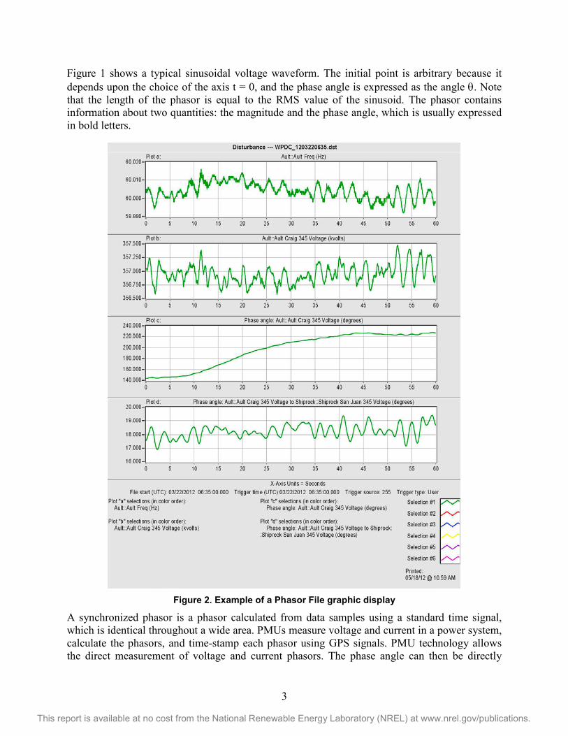
Figure 1 shows a typical sinusoidal voltage waveform. The initial point is arbitrary because it depends upon the choice of the axis t = 0, and the phase angle is expressed as the angle θ. Note that the length of the phasor is equal to the RMS value of the sinusoid. The phasor contains information about two quantities: the magnitude and the phase angle, which is usually expressed in bold letters.

Figure 2. Example of a Phasor File graphic display

A synchronized phasor is a phasor calculated from data samples using a standard time signal, which is identical throughout a wide area. PMUs measure voltage and current in a power system, calculate the phasors, and time-stamp each phasor using GPS signals. PMU technology allows the direct measurement of voltage and current phasors. The phase angle can then be directly

4


measured rather than calculated. Current PMUs can generate synchronized phasor measurements at 30 Hz. Faster PMU data rates enable observations and analyses of many grid and WPP dynamic behaviors that were not possible with the standard utility supervisory control and data acquisition (SCADA) system, which typically provides one measurement every 4 to 6 seconds (s). Because of their precise timing and higher data rates, synchrophasors have a huge potential to be used in future power system operations and planning.

An example of a synchrophasor data file is shown in Figure 2. Plot (a) shows the trace of frequency recorded by the Ault, Colorado PMU during a 1-min window. Plots (b) and (c) show the voltage magnitude and phase angle of the Ault–Craig, Colorado 345-kV line measured at Ault during the same 1-min window. Plot d shows the phase angle difference between the voltage phasors at Ault and Shiprock, New Mexico. The traces shown in Figure 2 are typical patterns of voltage phasors and frequency during normal operating conditions. The three electric grids of North America (Canada and the United States) are very reliable and have very stable system frequencies. As shown in Figure 2, the maximum frequency deviation from peak to peak was only 0.02 Hz (or 0.033%). The system frequency, voltage, and current experienced large changes only when abnormal operating conditions occurred.

Because all of the measurements are synchronized, PMU technology allows for wide-area monitoring. Power system monitoring includes the estimation of frequency and damping of oscillations induced by the interconnection of synchronous machines. With enough PMUs installed, the health of the entire power system can be monitored and evaluated before decisions need to be made about system protection and control. Currently, many of these decisions are based on local measurements and do not consider system-wide consequences of their actions, such as the system-wide blackouts that occurred in the Western Electricity Coordinating Council (WECC) in 1996 or in the Northeast in 2003. PMUs enable power system networks and component models to be evaluated for accuracy. Analysis of power system models may show voltage phase angles across the system that are much lower than actual measurements indicate. With PMU data, it is possible to derive, improve, and validate dynamic models of the generators, reactive compensation, and other critical components in a power system network.

Synchronized phasors give system operators and planners unprecedented insight into the grid and provide much better information for investigating interactions between WPPs and the grid. A new set of tools has been developed around PMUs and synchrophasor data that enable operators and engineers to make real-time system-stability assessments and post-event analyses. The U.S. Department of Energy (DOE), North American Electric Reliability Council, utilities, vendors, federal and private researchers, and academia are collaborating on the research, installation, and application of phasor data under the North American SynchroPhasor Initiative. Utilities are installing more than 1,000 new PMUs on the grid with support from the DOE Smart Grid Investment Grant; however, there is no concerted effort to put PMUs at large WPPs.

The many applications of PMUs are varied and broad, including:

• Wide-area monitoring – assessing the health of the entire power system before protection and control decisions need to be made

• Power system monitoring – monitoring system events, post-event analyses, power system state estimation, and oscillation frequency and damping

5


• Power system protection – detecting phase-angle instability, providing back-up protection for distance relays, and assessing the health of the whole system rather than only the local health

• Power system control – controlling high-voltage, direct-current systems; power system stabilizers; and Flexible AC Transmission System (FACTS); and enabling renewable energy power plants to provide damping of oscillations

• Power system model validation Reference [2] covers the synchrophasor data monitored within the Oklahoma Gas and Electric power network area. Detailed analysis includes several WPPs within the region. Reference [3] describes various algorithms for screening PMU data from power system events based on relative phase-angle differences between nodes monitored within the Electric Reliability Council of Texas (ERCOT).

1.2 Summary Recently, PMUs have been installed throughout the United States; however, the applications for planning and operating power systems are not yet fully utilized. The availability of synchronized phasor data from PMUs offers unprecedented opportunities for observing and analyzing WPP operations under normal and grid-contingency conditions. The analyses of PMU data from Oklahoma Gas and Electric provided several noteworthy results, as documented in reference [2]. The most noticeable finding was the subsynchronous resonance detected at some of the observed WPPs.

The remainder of this report is organized into three different subsections. Section 2 presents an overview of power system stability, and Section 3 discusses how PMU measurements are used to assess wind plant equivalent inertia, a technique that enables us to assess effective inertia without knowledge of generator parameters or the number of turbines within a WPP. Section 4 discusses how power system stability is investigated by observing power system oscillations (i.e., inter- and intra-area oscillations) on an IEEE four-bus benchmark power system network.

1.3 References [1] Phadke, A.G.; Thorp, J.S. Synchronized Phasor Measurements and Their Applications

(Power Electronics and Power Systems. ISBN-10: 0387765352, ISBN-13: 978-0387765358. New York: Springer Science Business Media, LLC, August 20, 2008.

[2] Wan, Y.H Synchronized Phasor Data for Analyzing Wind Power Plant Dynamic Behavior and Model Validation. NREL/TP-5500-57342, NTIS/GPO Number: 1067916. Golden, CO: National Renewable Energy Laboratory, 2013.

[3] Allen, A.; Santoso, S.; Muljadi, E. Algorithm for Screening Phasor Measurement Unit Data for Power System Events and Categories and Common Characteristics for Events Seen in Phasor Measurement Unit Relative Phase-Angle Differences and Frequency Signals. NREL/TP-5500-58611. Golden, CO: National Renewable Energy Laboratory, 2013.

6


2 WPP Stability Evaluation 2.1 Background Power system stability is the ability of an electric power system at a given initial operating condition to regain a state of operating equilibrium, with most system variables bounded so that practically the entire system remains intact, after being subjected to a physical disturbance [1].

Large power system disturbances are usually caused by severe system events (e.g., short circuits, loss of lines) and may lead to network changes during fault clearing when the faulted lines are temporarily disconnected from the network so that repairs can be performed. Small disturbances are usually caused by normal switching events (e.g., additional normal loads, capacitor switching) or self-clearing faults with no disconnection of the circuit breakers. This section describes how synchrophasor quantities (magnitude and phase angle) can be used to observe, detect, protect, and formulize remedial action schemes during contingencies.

Figure 3. Power system stability classification [1]

2.2 Rotor-Angle Stability Rotor-angle stability refers to the ability of synchronous machines in an interconnected power system to remain in synchronism after being subjected to a disturbance. It depends on the ability of each synchronous machine in the system to maintain and/or restore equilibrium between electromagnetic torque and mechanical torque. Instability that may result occurs in the form of increasing angular swings of some generators, leading to their loss of synchronism with other generators.

The change in electromagnetic torque of a synchronous generator in a post-fault operation can be categorized as a synchronizing torque component and damping torque component. A

7


synchronizing torque component is in phase with the rate of the rotor-angle deviation. This component affects the outcome of the post-fault, steady-state condition and may lead to non-oscillatory increases in rotor-angle instability and an eventual breakout from the system. A damping torque component is in phase with the speed deviation and may lead to increasing rotor-angle oscillations and eventual instability [1]. Power system oscillations indicated by rotor-angle oscillations are observable from the phase angle of the voltage measured at the bus (at the generating station) monitored by a synchrophasor (PMU).

Small-disturbance rotor-angle stability refers to maintaining angle stability after a small disturbance; large-disturbance angle stability is also called transient stability. Rotor-angle oscillations may occur between a single generator and the rest the grid (local plant oscillations), between a group of generators within the same balancing authority area (intra-area oscillations), and between a group of generators in different balancing authority areas (inter-area oscillations). Rotor-angle oscillations affect the rotating electric machines connected to the same grid, develop mechanical stress within the path to the mechanical loads (shaft, gearbox, mechanical coupling, etc.), and are usually of a short duration (< 20 seconds). Most large synchronous generators are equipped with power system stabilizers to quickly damp out the oscillations by controlling the excitations of the generator to reduce angle oscillations via rotor-speed feedback.

2.2.1 Loss of Line In steady-state conditions, the voltage at the two buses (VA and VB) is usually maintained constant near 1.0 p.u. by controlling the excitation of the generator. The relative phase angle between two buses, also called the power angle δ, is an indication of the power level transfer between two buses. In the power system shown in 4 (a), there are power transfers from Bus A (sending end) to Bus B (receiving end) through three parallel lines. To simplify the analysis, we assumed that the resistance in the transmission lines was negligible, thus the impedance considered was only the reactance X.

Line 1

Line 2

Line 3

VA VB

(a) Parallel transmission lines (b) Power-angle curve between two buses

Figure 4. A simple two-bus system illustrating rotor-angle dynamic stability [2–3] Equation 2 describes how the power transfer is dependent on the voltage magnitudes of Bus A and Bus B, the equivalent line impedance between Bus A and Bus B, and the voltage phase-angle difference between Bus A and Bus B.

𝑃 = |𝑉𝐴||𝑉𝐵|𝑋

sin 𝛿 (2)

8


Figure 4 (b) shows the power-angle relationship. As the power transfer increases, the voltage phase-angle separation grows. But there is a limit to the amount of power that can be transferred (indicated by the dashed red at δ = 90°). If the power transfer from Bus A to Bus B is fixed at the line set on the graph, the phase angle is equal to δ1. If a disturbance occurs, it can cause both the power and phase angle to oscillate along the curve, as shown by the red arrows around P1. Thus, the closer the oscillations come to the stability limit (δ = 90°), the less the system can tolerate.

When all of the lines are operating at a normal condition, the operating point is at point P1 and δ1. The generator G1 is supplying load (PL) at bus G2. Any small disturbance will perturb the operating point around the equilibrium P1. The system is stable if for any perturbation the post-disturbance operating point returns to the same point P1, δ1. The Positive Sequence Load Flow (PSLF, developed by General Electric) dynamic simulation tool is used to illustrate disturbance events. Note that the steady-state illustration presented by the power-angle curve in Figure 4 (b) and the phasor diagram shown below in Figure 6 are simplified to describe the changes that occur during transients. The actual dynamic of the power system includes the generator excitation, nonlinearity of the magnetic saturation, kinetic energy changes, exciter upper and lower limits, and many other dynamics that come into play.

As one line is disconnected, the impedance X increases and the power transfer capability decreases; thus, the power-angle curve shrinks and the operating point of G1 moves from point P1, δ1 to point P’1, δ1. The load demand stays the same (PL), and because there is a difference between the load and the generation, the power angle δ and the operating point will move. Because of the rotating inertia of the generator, the operating point first moves to P’1 (on the new power-angle curve) at a constant power angle δ = δ1, thus generating less than the load demand PL. This difference will force the generator to increase its output power to match the load demand. As the power angle increases, the operating point moves toward P2, but it may overshoot, reaching P1”. It oscillates around P2, and the system damping makes it finally settle at P2. Note that the new power angle is larger than the previous one (δ2 > δ1) because the new impedance XNEW is higher than the old impedance X when one of the parallel lines is removed.

Figure 5. Voltage and power angle δ illustrating the dynamic when one line is out of service

V1

δ1 V2 = V1

δ2 > δ1

One line is disconnected

9


To illustrate the disconnection of one of the parallel lines, Figure 6 shows phasor diagrams representing voltage, voltage drop, and current. Figure 6 (a) illustrates the condition when all of the parallel lines are in service. Assume that the voltages at both buses are maintained close to per-unit values by the synchronous machines. When one of the parallel lines is disconnected, the impedance X increases to XNEW and the power transfer capability shown in Figure 4 (b) shrinks. The voltage drop across the transmission line increases in proportion to the size of the new impedance. The amount of power transmitted stays the same (P2 = P1), and the additional voltage drop on the transmission lines causes the power angle δ to increase from δ2 to δ1. As the exciter of the generator continues to maintain the voltage to counter the additional voltage drop, the reactive power output increases because of the additional reactive losses in the transmission lines (I2X).

(a) Small impedance (i.e., all lines are in service)

(b) Large impedance (i.e., one line is out of service)

Figure 6. Voltage phasors for two differently-sized line impedances Figure 6 helps explain the time series plots of the voltage and power angle shown in Figure 5. The plots of the real and reactive power, as shown in Figure 7, illustrate the dynamic behavior of the system when one of the lines is tripped or taken out of service. Note the change in the reactive power needed to offset the additional voltage drops caused by the higher impedance presented when one of the lines tripped offline.

Figure 7. Dynamic behavior of real and reactive power during one line removal

P1

P’1

P2 = P1

Q1

Q2 > Q1

P”1

VA

VB I

jIX δ1

VB

VA

jIXNEW I δ2

10


As shown in Figure 4 (a), if another fault occurs on the second line, the removal of the other two lines will cause the line impedance to become even larger than before and the power-angle curve to shrink even more. The operating point will move from point P2, δ2 to point P’2, δ2, and as the load demand PL stays the same, the power angle δ increases and passes the stability limit δ > 90°. The terminal voltage oscillates down to 0.725 p.u. and increases up to 1.16 p.u., and the system becomes unstable and loses its synchronization.

Figure 8 shows the plots of voltage and angle (the phasor quantities of the generator voltage) when the generator loses its synchronization. The generator is unable to supply the load demand when the impedance becomes very large when two of the three parallel lines are taken out of service at t = 1 second. The power angle δ (red curve) and the stator current increase, and the voltage drop across internal impedance Xs increases, further reducing the terminal voltage (blue curve) of the generator, which further shrinks the power-angle curve. The pole slipping during the nonsynchronous condition is shown in the severe voltage oscillations. In reality, the entire generator control system—including other quantities such as real and reactive power, torque, and rotational speed—are affected. The excitation will hit the upper and lower limits. Usually, the system protection relays (voltage, current, frequency, excitation, etc.) will kick in within a few cycles to disconnect the generator from the grid and protect the electrical and mechanical integrity of the generator during severe disturbances.

Figure 8. Voltage and power angles of an unstable post-transient illustrating the removal of two of

the three parallel lines

2.2.2 Self-Clearing Faults In this section, we investigate the nature of a self-clearing fault. A self-clearing fault involves a fault in which the lines are grounded but no lines are disconnected from the circuit. For example, a tree branch might touch high-voltage transmission lines, which would cause the branch to short circuit, burn, and dry, and the short circuit would be removed by itself. Another example is if two or more lines were touching each other because of heavy wind. This type of event usually lasts a very short time; however, it may cause a generator (or a group of generators) to lose its synchronization to the grid. The following diagram was computed and drawn in the PSLF

V1 = 1.05 p.u.

δ1 = 360o

δ1 = 90o

V1 = 0.725 p.u.

V1 = 1.16 p.u.

11


platform. It shows the power flows, power losses, bus voltages (both in real-value and in per-unit quantities), and status of the switches.

Figure 9. Voltage, real, and reactive power computed by the power flow program (PSLF)

The single-line diagram shown in Figure 9 illustrates the five-bus system under study. The generator is connected to a step-up transformer and then to a sub-transmission line. At the substation transformer, the voltage is stepped up to 240 kV and the power is transmitted over two identical parallel lines (equal impedance). The power flow is computed using PSLF. The real (top numbers) and reactive power (bottom numbers) flow in the lines and transformers are shown in pairs. The computed bus voltages are also shown in the single-line diagram.

Figure 10 shows two power-angle curves illustrating two different events with two different durations of faults. Figure 10 (a) shows a stable operation. When the fault occurs, the terminal voltage drops to zero and the output power goes to zero; thus, the generator accelerates, the power angle moves from δ1 to δ2, and the operating point moves from point P1 to P2 to P3. When the fault is cleared, the voltage is returned to normal, the output power of the generator is restored, and the generator operating point moves to P4. However, because of the generator inertia, the acceleration cannot be reversed instantaneously, so the operating point moves farther to point P5, at which point the generator starts to decelerate, which moves the operating point back to P4, P1, overshooting P6. After some power oscillations, eventually the system returns to the final resting point, at P1, the power before the fault occurred. Because this fault is a self-clearing fault, the size of the impedance does not change before and after the fault; thus, only a single power-angle curve is needed. Figure 10 (a) presents a system that remains stable in the post transient.

Equal-area criterion of stability is used to predict the stability of a power system [2–3]. Equal-area criterion of stability is based on an equal area within the power-angle curve. The blue area in Figure 10 (a) shows the area under the mechanical power of the prime mover (equivalent to load demand PL) when the output power of the generator drops to zero as the terminal voltage drops to zero for the duration of the fault. The blue area represents the acceleration when the mechanical power drives the generator during the fault (i.e., desynchronizing area). The red area shown in Figure 10 (a) represents the restoration to normal operation during deceleration when the generator power is restored at a higher level after the fault is cleared (i.e., synchronizing power area). The system is considered stable when there is enough red (restoring power) to overcome the blue.

The corresponding phasor diagram in Figure 10 (b) shows that the phasor voltage at the sending end moves phasor VA from δ1 to δ2, and that after the fault is cleared, the angle continues to

12


increase, reverses direction, and, after small oscillations around the normal operating point, finally settles back to the original operating point at P1, δ1. Figure 10 (b) also shows that the voltage magnitude drops to practically zero.

(a) Power-angle curve for equal-area

stability assessment (b) Phasor diagram of the voltage during a

transient

Figure 10. Steady-state angle stability assessment—stable operation

The event is illustrated by presenting the results of the dynamic simulation shown in Figure 11. The voltage magnitude and the phase angle are shown in Figure 11 (a). During the pre-fault condition, the power angle is δ = δ1 and the corresponding voltage is VA = V1. At time t = t1, the fault is initiated, and the fault self-clears after nine cycles. Meanwhile, the power angle reaches δ = δ2 just before the fault is cleared at time t = t2. The voltage actually drops down to V2 during the fault. Figure 11 shows that the voltage does not go all the way down to zero, indicating that there are impedances (line and transformer) between the fault (Bus 2) and the terminal of the generator (Bus 5). As a result, the terminal voltage does not reach zero; instead, V2 = 0.46 p.u. because of the voltage drop developed by the short-circuit current across the impedance. Figure 10 (b) shows the real and reactive power traces. The real power drops to a very low value, and the reactive power goes very high during the fault. As expected in a self-clearing fault, the voltage and the phase angle finally return to the pre-fault values.

Under normal circumstances, the voltage at the buses is usually maintained close to per-unit values with limited variation (0.9 < V < 1.1 p.u.). Allowing the voltage to go beyond the range would require more expensive transmission infrastructure (insulators, structures, ride-of-way, etc.) and would disturb or damage customer loads. For a self-clearing fault, there is no line removal from the network; thus, there is no impedance change during and after the fault. We deal with only one power-angle curve.

VB

VA

jIXNEW δ1 δ2

13


(a) Voltage magnitude and corresponding angle

(b) Real power and reactive power

Figure 11. Self-clearing fault for a duration of nine cycles

Next, if we observe the translation of the power angle δ, it passes 90° and reaches the maximum, 122°. Consider the mechanism that makes the size of the desynchronizing power area (blue area) increase. The square blue area is determined by the initial load demand power (P1 = PL) and the phase-angle shift (∆δ = δ1- δ2) for the duration of the fault (∆tFAULT = t1 - t2) before it is self-cleared. At the same time, we can also consider the condition that limits the size of the restoring power area (red area). The higher the initial power, the smaller the potential size of the restoring power area. Also, the wider the phase-angle shift (∆δ), the smaller the potential size of the restoring power area (red area). The phase-angle shift is determined by the rotational inertia of the generator and the initial (pre-fault) output power of the generator. Thus, for any set of conditions there will be a critical clearing time (∆tCR = the length of time it takes to clear the fault) [5]. If the fault is not cleared after ∆tCR = 14.6 cycles, the system can become unstable.

δ1

δ2 = 80ο

δ1

V1

V2

V1

δ = 122ο

14


The phase shift corresponding to ∆tCR is the critical clearing angle ∆δCR. Figure 12 shows the voltage phasor of an unstable system operation. The blue area in Figure 12 (a) is large, and there is not enough space between the power-angle curve and the load demand to counter the blue area (blue area > red area). The power-angle curve indicates an unstable condition. As shown in Figure 12 (b), the phasor swings past 180° and never returns to normal operation.


criterion of stability (b) Phasor diagram of the voltage during a

transient

Figure 12. Steady-state angle stability assessment—unbstable operation

Figure 13 shows the traces of voltage magnitude and the corresponding angle for a stable operation at its stability limit. In this case, the critical clearing time was found to be 14.1 cycles. The corresponding critical clearing angle, from the fault inception to the time the phase angle changes, is 48°. Any delay in clearing the fault will cause the system to become unstable and the voltage magnitude and angle will show some oscillations before settling to their original values.

Figure 13. Voltage magnitude and corresponding angle (stability limit) of the self-clearing fault at the critical clearing time

VB

VA

jIXNEW

∆δCR

VA

δ

δ1

δ2 = 113ο

V2 = 0.34 p.u.

δ = 168ο

∆δCR=48o

∆tCR=14.1 cycles

15


2.2.3 Line Opened to Clear the Fault In this section, we investigate a case in which the fault is cleared by opening the affected line. Clearing the fault this way removes the fault from the network, but it changes the network structure and thus the characteristic of the circuit. The single-line diagram shown in Figure 14 was computed and drawn in the PSLF platform. It includes the power flows, power losses, bus voltages (both in real value and in per-unit quantities), and status of the switches. As shown, one of the parallel lines is opened, and it makes the impedance of the transmission line between Bus 1 and Bus 2 significantly larger than when both lines are in service. It forces all of the current to flow in the remaining line, the loading of the lines increases, and the power line loss (the power difference between the sending end and receiving end) is significant. The developed voltage drop is also shown to increase significantly. To appreciate the differences, compare Figure 9 to Figure 14.

Figure 14. A single-line diagram illustrating a line opening to clear a fault

Figure 15 shows the power-angle curve to illustrate the fault clearing by opening the line. The opening of the line involves changing the line impedance; thus, two sets of power-angle curves are shown. One corresponds to the normal operation of the system; the other corresponds to the one with a disconnected line (to clear the fault).


criterion of stability (b) Phasor diagram of the voltage during

a transient Figure 15. Steady-state angle stability assessment (line opened to clear a fault) during the critical

clearing time

As discussed above, the case discussed here is related to opening the fault to clear it. The fault is cleared at the stability limit (critical clearing time) [2–3]. A very small delay in clearing the fault will develop into an unstable operation in the power system network. As expected, the critical clearing time for this case (∆tCR = 12.6 cycles) is shorter than that in the self-clearing fault (∆tCR

VA

VB

VA jIXNEW

δ2

VA

δP5

δ3 δ1

∆δCR VA

δ3

16


= 14.6 cycles). Because of the shrinkage of the power-angle curve resulting from the increase of the line impedance (X=XNEW), the opportunity to balance the size of the desynchronizing power area (blue area) becomes smaller while the potential restoring area (red area) gets smaller.

The sequence of operation goes from P1 (normal operation), to P2-P3 (during the fault), to P4 to restore the operation after the fault (new power-angle curve), to P5 (the stability limit), back to P4–P6, returning to normal operation at P1’. Note that there is an oscillation along the power-angle curve (before the operating point settles at the point P1’). The phasor diagram shown in Figure 14 (b) is intended to complement the illustration presented in Figure 14 (a).

(a) Voltage magnitude and the corresponding angle

(b) Real power and reactive power

Figure 16. Fault clearing by opening the line (∆tCR = 12.6 cycles)

The dynamic simulation is performed to verify the steady-state prediction illustrated in Figure 16. As shown in Figure 16 (a), the voltage magnitude follows the prediction, the voltage drops to 0.46 p.u. during the fault, and the magnitude swings as the rotor angle oscillates. When the oscillation is finally damped out, the voltage returns to its initial voltage. The final power angle is δ3 =78°, the initial angle is δ1 =66°, and the phase angle at the end of the fault is δ2 =78°. The power angle swings between δMIN = 40° and δMAX = 152°.

δ1= 66ο δ2 = 78ο

V2 = 0.46 p.u.

δ = 152ο

∆δCR=12o

∆tCR= 8.38 cycles v1

δ = 40ο

δ3 = 78ο

P’1 = 100.3 MW P1 = 100 MW

Q’1 = 24 MVAR Q1 = 3.6 MVAR

17


In Figure 16 (b), the real and reactive power follows the trend shown by the voltage phasors. The output power initially set at 100 MW drops to a very small value during the fault (11 MW). After the fault, the output power swings until it finally settles at approximately 100.3 MW, which can be expected because of the additional voltage drop in the transmission line as a result of the one line that was tripped. The reactive power was originally 3.6 MVAR. During the fault, the exciter of the generator tries to compensate for the voltage drops, it oscillates following the rotor-angle oscillations after the fault is removed, and after the oscillation is damped out, the reactive power settles at 24 MVAR. Note that the additional reactive power is expected when the line impedance increases with the removal of one of the parallel lines.

2.2.4 Example Using the WECC Network As an illustration, we move from a very simple model discussed previously to a real WECC network. We selected a case from the WECC website for heavy summer 2015. We observed concentrating solar power modeled as a steam power plant in the southwestern United States during normal faults. Keep in mind that in power systems the circuit breakers and relay protections are used to isolate faults to minimize the affected loads from regular faults.

In the previous examples, we assumed that we had a two-bus system in which one of them was an infinite bus (Bus B). An infinite bus is assumed to have an ideal voltage source with a very large inertia and a very fast response exciter circuit maintaining a constant voltage at all times. Thus, for the two-bus systems in the previous examples, the phasor voltage at Bus 1 was always represented as VB = VINFINITE = 1.0 / 0o p.u. As shown in Figure 17, with a large system such as WECC, usually only one generator is considered as an infinite bus. The rest of the generators are free to change with respect to the infinite bus. Thus, the rest of the circuit has a voltage phasor dynamically affected by any dynamic event. The power angle δ2 is the result of the phase-angle difference δ2 = δA - δB in which both phasors VA and VB are dynamically changing during a disturbance. In a muti-bus system, the dynamic is not only determined by the inertia and damping of the single generator A, but also by the inertia and damping of the rest of the systems.

Figure 17. Phasor diagram of a single generator connected to an infinite bus and a large multi-bus system

We use the LVRT minimum requirement for WPPs as described in the Large Generator Interconnection Agreement of Appendix G in the Federal Energy Regulatory Commission’s Order 661 [4]. The generator shall not be disconnected when subjected to the voltage profile at the point of interconnection (refer to Figure 18). In a WPP, the point of interconnection is the

VB= Vinfinite

VA

jIX

VB

VA

jIX

δΒ

δΑ

δ1

δ2 δΑ

Vinfinite

V5 V1 jX

to the rest of system

to the rest of system

(a) Simplified diagram (b) Two-bus system (c) Large system with multi buses

18


high side of the substation transformer, with the voltage level usually at 110 kV, 230 kV, or above. The LVRT is intended to ensure that the generator stays connected to the grid when there is minor disturbance. If the power plant is taken out of lines for a small disturbance, there is an imbalance between the load demand and the generation supply. This creates frequency decline, which may further trigger other generators to trip offline. This sequence of events may get worse and lead to an eventual blackout.

Figure 18. The LVRT requirement per the Large Generator Interconnection Agreement in Appendix

G of the Federal Energy Regulatory Commission’s Order 661

Figure 19. Voltage and frequency at the point of interconnection and the LVRT drawn on the same

figure

Because it is not possible to simulate fault that will have the exact voltage profile shown in Figure 19, we simulate a nine-cycle (0.15-sec), three-phase fault at the point of interconnection, and observe the phasor of the voltage at the generator terminals. Figure 19 shows the simulation results of the voltage at the point of interconnection. The voltage profile of the LVRT is drawn on the same figure for reference. The frequency measured at the point of interconnection is also shown on the same figure. The voltage at the point of interconnection varies in a damped oscillation with a maximum 1.066 p.u. The frequency oscillation is shown to have a minimum frequency of 59.65 Hz and a maximum frequency of 60.27 Hz.

LVRT

VPOI VMAX

fMAX fPOI fMIN

19


Figure 20 shows the simulation results of the voltage and the angle at the generator. The voltage drops to VMIN = 0.46 p.u. and swings in a damped oscillation, reaching VMAX = 1.1 p.u. Although the voltage at the point of interconnection reaches zero during the fault, the voltage upstream from the fault is always higher because of the voltage drop across the impedance between the fault and the generator. The generator angle was δ = 60° before the fault was initiated. After the fault, the angle swings between δMIN = 19° and δMAX = 121°.

Figure 20. Voltage and angle at the generator

Figure 21. Real power and reactive power dynamic

Figure 21 shows the simulation results of the real power (P) and reactive power (Q) output of the generator. The output power of the generator is initially at P = 30 MW, it reaches down to 3 MW during the fault, and recovers with an oscillation of the output power between PMIN = 13 MW and PMAX = 48 MW. The reactive power output of the generator was at PMIN = 0 MVAR before the fault was initiated. During the fault, the generator generates max reactive power to support the voltage drop, and the reactive power reaches PMAX = 31 MVAR. After the fault, the reactive power oscillates following the trend of the generator voltage, which indicates that the field

VMAX VMIN

δMAX δ δMIN

QMAX Q

PMAX P PMIN

20


excitation of the generator works to compensate the voltage deviation from maintaining its target value of maintaining 1.0 p.u.

2.2.5 Example Using a WPP in the WECC Network CPPs have an advantage over WPPs in their independent locations regardless of a wind resource. CPPs are usually located close to load centers to minimize the length of the transmission lines from the generators to the loads; thus, the line impedances and line losses are also minimized. The location of a WPP is usually chosen to be at sites with high wind resources. In some cases, WPP output must be transmitted over long distances (long transmission lines equal weak grids). Another advantage of CPPs is the controllability of their output power, ranging from the maximum power to the minimum power specified by the manufacturer. The level of generation is adjustable to follow the load, thus balancing the real power is done by simply following the load demand. A WPP owner wants to harvest as much wind energy as possible; thus, the level of generation varies with the availability of the wind speed. In some cases, the level of wind generation must be curtailed to accommodate the available transmission capacity and the reliability of the power system operation. Wind generator power output can only be controlled to be less than the available wind average; it cannot be raised up above the available wind speeds.

One advantage of a WPP over a CPP is its redundancy. There are hundreds of turbines within a WPP covering a very large area (creating diversity in wind speed at each turbine, and diversity of line impedance, or electrical distance, from each turbine to the point of interconnection); thus, during fault events only a few percentages of the turbines are disconnected from the wind plant [5]. A CPP consists of a large generator; thus, during a fault event the entire generation may be disconnected from the power grid. Another advantage of a WPP is that it is made up of modern wind turbine generators employing power converters (power electronics) to operate in variable speed to optimize the wind harvest and thus maximize output. With the availability of power electronics in the generating system, flexible reactive power deployment can be accomplished, thus voltage control is easily implemented. Also, grid integration and power quality in WPPs is superior to CPPs because real and reactive power can be controlled independently and instantaneously. Power electronics allow the level of real power generation to be adjusted to help damp a system during oscillation, thus the stability of the power system can be improved.

A WPP’s practical limits are usually very flexible; however, it follows the general requirements of a CPP. From the real power perspective, a modern WPP can provide spinning reserves, inertial response, frequency response, and governor control. Similarly, from the reactive power controllability, a WPP has the capability to adjust reactive power. The level of reactive power in a modern WPP is usually within a range of +/- 0.95. The voltage in a WPP is within a range from 0.95 p.u. to 1.05 p.u. during normal operation. During transient and short-term disturbances, the voltage is usually allowed to vary between 0.9 p.u and 1.0 p.u.

21


Table 1. Comparison Between a CPP and a WPP

2.2.6 Example Using a WPP in the WECC Network Another example is taken from a WPP in the WECC network. This WPP is rated at 204 MW and consists of 136 Type 3 wind turbine generators, each rated at 1.5 MW. This turbine is a variable-speed turbine and is operated during a typical heavy summer 2015 with an output of 10 MW (low-wind condition). Dynamic models commonly used for wind turbine generators and WPPs were developed by WECC’s Renewable Energy Task Force and implemented by several software vendors (PSSE by Siemens PTI, and PSLF by General Electric) [6–7]. Figure 22 illustrates a small subset of WECC network systems. It shows the power system network of the system under investigation. Thousands of buses, transmission lines, transformers, and capacitors comprise the WECC network. The fault at Bus 10999 was cleared after nine cycles. There are no additional reactive power compensations at the turbine level and at the plant level. The voltage and angle at the point of interconnection are shown in Figure 23.

Figure 22. Single-line diagram of a WPP and nearby buses

Fault to 13402

to 10025

to 10991

Conventional Power Plant Single large (40-MW to 100-plus

MW) generator Prime mover: Steam, combustion

engine – non-renewable fuel Controllability: Adjustable up to max

limit and down to min limit

Located where convenient for fuel and transmission access

Generator: Synchronous Fixed speed – No slip: Flux is

controlled via exciter winding. Flux and rotor rotate synchronously

Wind Power Plant Many (hundreds of) wind turbines (1-MW

to 5-MW each) Prime mover: Wind turbine – wind Controllability: Curtailment, ramp rate

limit, output limit Located at wind resource, may be far

from a load center Generator: Four different types (fixed

speed, variable slip, variable speed, full converter)

Type 3 and Type 4: Variable speed with

flux-oriented controller via a power converter. Rotor does not have to rotate synchronously

22


The traces of the voltages and the corresponding angles are shown in Figure 23. The corresponding voltage phasor diagram based on the phasor information is shown in Figure 24.

Figure 23. The voltage and angle at the wind turbine generator

Figure 24. Voltage phasor diagram

The voltage phasors shown in Figure 23 have a very large phase-angle shift (also known as a phase jump) from a normal condition at Point A to short-circuit conditions at Point B and Point C. This is expected in short-circuit conditions because of the changes in the circuit impedance during the fault. The current phasor diagram shown in Figure 24 was reconstructed from the real and reactive power components of the output currents. The red represents the real power component, the blue represents the reactive power component, and the black represents the resultant current passing through the insulated-gate bipolar transistors (IGBTs) of the power converter. Note that in Type 3 and Type 4 wind turbines, the output characteristics of the generators are controllable via the power converter. Thus, we can command the power converter to generate real and reactive power independently and instantaneously. As shown in Figure 24, the reactive current is maximized to help support the voltage dip during the fault. Additional studies on this subject can be found in the references [8–9].

Figure 25. Real and reactive power components of the currents

VWTG VMIN =0.33 p.u.

δWTG = 2.9o δMIN = -167o

A

B

C

D

D E

E

A

B C

A

B C

D E

reference

A, E B

B

C

B

reference

CURRENTS

VOLTAGES

NOTE THE ABSENCE OF ROTOR ANGLE OSCILLATIONS IN THE POST-FAULT REGION

23


Note, in Figure 25 the real and reactive components of the output current are shown to have a dramatic change during the fault as the reactive currents surges up to support the voltage dip caused by the fault.

In a conventional synchronous generator, this sudden phase jump creates a sudden stator flux jump in the air gap of the generator, which creates a sudden power-angle jump with respect to the rotor flux (attached to the rotor poles). Because of the rotor inertia, it takes some time for the rotor to follow the stator flux. This results in large torque spikes, which trigger the rotor-angle oscillation immediately after the fault.

Figure 26. Real and reactive power output of the generator

In a doubly-fed induction generator, the power converter is fed to the rotor winding via slip rings, and the output current can be controlled to follow the stator flux; thus, the power angle of the generator does not jump nor create a large torque spike. Instead, the output power can be controlled constant, and, at the same time, the reactive power can be maximized. Note that this particular doubly-fed induction generator (DFIG) wind turbine is set to have an approximate 125% overload current capability. This current-carrying capability is very important in a power converter because of the limitation of the current-carrying capability of the IGBTs. Figure 26 shows the real and reactive power output of the generator. Note that the reactive power is controlled to maximize the utilization of the IGBTs during the fault to support the voltage dip.

2.3 Voltage Stability Voltage stability refers to the ability of a power system to maintain steady voltages at all buses in the system after being subjected to a disturbance from a given initial operating condition. Voltage stability depends on the power system’s ability to maintain and/or restore equilibrium between load demand and supply. Instability that may result occurs in the form of a progressive fall or rise of voltages of some buses.

A possible outcome of voltage instability is the loss of load in an area or the tripping of transmission lines and other elements by their protective systems, leading to cascading outages. Loss of synchronism of some generators may result from these outages or from operating conditions that violate a field current limit. Voltage stability may vary during the duration of the event; it can be short term (< 1 minute) or it may evolve during many hours [10–11].

24


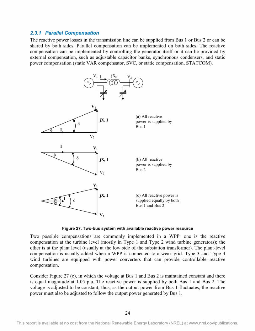
2.3.1 Parallel Compensation The reactive power losses in the transmission line can be supplied from Bus 1 or Bus 2 or can be shared by both sides. Parallel compensation can be implemented on both sides. The reactive compensation can be implemented by controlling the generator itself or it can be provided by external compensation, such as adjustable capacitor banks, synchronous condensers, and static power compensation (static VAR compensator, SVC, or static compensation, STATCOM).

Figure 27. Two-bus system with available reactive power resource

Two possible compensations are commonly implemented in a WPP: one is the reactive compensation at the turbine level (mostly in Type 1 and Type 2 wind turbine generators); the other is at the plant level (usually at the low side of the substation transformer). The plant-level compensation is usually added when a WPP is connected to a weak grid. Type 3 and Type 4 wind turbines are equipped with power converters that can provide controllable reactive compensation.

Consider Figure 27 (c), in which the voltage at Bus 1 and Bus 2 is maintained constant and there is equal magnitude at 1.05 p.u. The reactive power is supplied by both Bus 1 and Bus 2. The voltage is adjusted to be constant; thus, as the output power from Bus 1 fluctuates, the reactive power must also be adjusted to follow the output power generated by Bus 1.

V1 V2 I jXs

V1

V2 I

jXs I (a) All reactive power is supplied by Bus 1

(b) All reactive power is supplied by Bus 2

V1

V2

I

jXs I

V1

V2

I jXs I (c) All reactive power is

supplied equally by both Bus 1 and Bus 2

φ

δ φ1 φ2

φ

δ

δ

25


In this case:

φ1 = φ2 = δ/2

Thus, the reactive power generated by Bus 1 must follow:

Q = V1 I sin (δ/2)

And the reactive power can be commanded to follow the rules:

Q = P tan (δ/2)

P = V2 sin δ /Xs

With an active adjustment of reactive power generated by reactive power compensation at Bus 1 and Bus 2, the voltage level can be kept constant at varying wind power output. Note that this control helps to keep the voltage adjusted, but the power angle δ is not affected for the same amount of power delivery. Figure 28 shows an example of controlling reactive power to maintain equal contribution of reactive power from both sides of the buses.

Figure 28. Voltage phasor diagram with equal contribution of reactive power from both sides

2.3.2 Series Compensation The reactive power compensation can also be accomplished by using series compensation (refer to Figure 29). The advantage of series compensation is that the voltage and current rating of the series compensation is relatively small considering that it is intended to compensate for the voltage drop of the line impedance. Series compensation is commonly used to compensate long transmission lines; however, care must be taken not to make it prone to cause subsynchronous resonance.

V1

V2

I jXs I

V1

V2

I jXs I

δ

(a) Low wind speeds

(b) High wind speeds

26


Figure 29. Single-line diagram of a series-compensated system and a diagram of its voltage phasor

Figure 30. WPP represented by a single generator

A typical WPP representation is shown in Figure 30. Note that the equivalent generator, pad-mounted transformer, and collector system can be easily derived from the actual collector system schedule [12–15].

2.3.3 PV and VQ Curves In this section, we show how to perform power-voltage (PV) and voltage–reactive power (VQ) power system stability analysis on a WPP. We use a single-turbine representation of a WPP. The WPP uses 1.5-MW Type 3 wind turbines (variable-speed DFIG) operated in variable-speed mode with a constant power factor, PF=1.0. The total output power of the WPP is rated at 204 MW. The WPP is connected to the rest of the power system via its point of interconnection. Two grid conditions are used in this study: one is the stiff-grid and the other is the weak-grid condition. The stiff-grid condition is simulated by connecting both of the transmission lines between Bus 1 and Bus 2. The weak-grid condition is simulated by disconnecting one line of the parallel lines between Bus 1 and Bus 2. The transmission lines are overhead lines with a very small shunt capacitance.

V1 V2

I jXs

jXc V1C

By adjusting XC = 0.5 Xs, it is possible to generate an improved power factor at Bus 1 and reduce the power angle δ between Bus 1 and Bus 2 for the same power delivery.

V1C V1

V2

I

jXC I

δ

Gen

100-MW Equivalent Wind Turbine Generator

Infinite Bus

Ideal Gen

230-kV Line 1 R1, X1, B1

230-kV Line 2 R2, X2, B2

34.5-kV Collector System Equivalent Re, Xe, Be

0.6/34.4-kV Equivalent GSU Transformer Rte, Xte

34.4/230-kV Station Transformer Rt, Xt.

Station-Level Shunt Compensation

Turbine-Level Shunt Compensation

2 1 3

4

5

27


The collector system is built with underground cables and some overhead lines. Because the size of the WPP area is very large, the length of the cable connecting individual turbines is different for each turbine.

2.3.3.1 PV Capability Curve A PV capability curve is normally conducted to measure the proximity of the rated operating condition of a WPP to the voltage collapse. In a large power system network, the level of the output power of a group of generators in the area and zone of interest are usually varied and the other group of generators is reduced by the same amount of power to develop net-zero additional output power. For a WPP, a PQ characteristic map of the WPP is generally used and the WPP is operated from a low-wind to higher-wind condition with a pair of P&Q from the PQ characteristic map. Most wind turbine generators (Type 1 and Type 2) are normally compensated to have a unity power factor operation by using a switched capacitor. Type 3 and Type 4 wind turbine generators are built with the capability to vary reactive power and can be operated to control voltage, reactive power, or the power factor output via a power converter control. Additional information related to PV and VQ curves as discussed in this section and the next section can be found in the references [10–11].

Figure 31. Voltage at the generator for stiff-grid and weak-grid conditions

In this investigation, we operate a Type 3 wind turbine at a unity power factor, thus generating only real power at its terminals. No other reactive power compensation is provided at the turbine level or at the wind plant level. The PV curves shown in Figure 31 were derived by measuring the bus voltage at the generator as we varied the output power of the wind turbine. As shown in Figure 31, both the weak grid and stiff grid are shown on the same figure. The real power margin for the grid is measured from the rated power (P = 1.0 p.u.) to the knee point where the voltage collapses. Using PSSE or PSLF, it is easy to find. Usually the computation does not converge beyond the knee point. In the simple case we study, the real power margin for the stiff grid is Pmargin-STIFF = 1.4 p.u. (= 280 MW) at voltage V = 0.77 p.u. Similarly, the real power margin for

0.7

0.75

0.8

0.85

0.9

0.95

1

1.05

0.5 0.7 0.9 1.1 1.3 1.5

Volta

ges

at G

ener

ator

(p.u

.)

Real Power (p.u.)

PV Curve

Voltage @ WTG Stiff-GridVoltage @ WTG Weak-Grid

Pmargin-WEAK

Pmargin-STIFF

1.0

28


the weak grid is Pmargin-WEAK = 1.1 p.u. (= 220 MW) at voltage V = 0.82 p.u. The voltage characteristic of the voltage indicates that for a stiff grid we can increase the level of generation to 125% of rated power while keeping the bus voltage above 0.9 p.u. However, for a weak grid the level of generation can be adjusted up to 97% rated before the voltage drops below 0.9 p.u.

Figure 32. Reactive power comparison at the infinite bus for weak-grid conditions

The wind turbine generators are operated in unity power factor mode; thus, there is no reactive power supplied by the generator to the grid to compensate for the reactive losses within the collector systems inside the WPP, in the transformers, and the transmission lines. As shown in Figure 32, the reactive power losses are supplied by the grid (Bus 1 as the infinite bus). In both cases, the reactive power is shown to exhibit a nonlinear (slightly quadratic) function of the wind plant output power, which is expected. Note that the reactive power needed for an output of 1.0 p.u. real power is 38% rated power for a stiff grid and 56% for a weak grid.

The above exercise is conducted by setting the generator to produce a unity power factor output power. It will give different results if the WPP is operated at different modes (e.g., constant power factor, constant voltage, constant reactive power).

2.3.3.2 VQ Capability Curve A VQ capability curve is normally investigated to determine the reactive power adequacy in a WPP. Reactive power capability is an important aspect of controlling the voltage and influencing the PV characteristic behavior.

As mentioned previously, the WPP uses Type 3 wind turbine generators. All of the wind turbines are controlled to regulate Bus 3 (low side of the substation transformer). The setting point of the regulated voltage is varied from 0.6 p.u. to 1.0 p.u., and the reactive power is plotted against the regulated voltage. The grid voltage (infinite bus) is set to1.05 p.u. all the time, and the generator real power output is set to 1.0 p.u.

0

0.2

0.4

0.6

0.8

1

1.2

1.4

0.5 0.7 0.9 1.1 1.3 1.5

Rea

ctiv

e Po

wer

(p.u

.)

Real Power (p.u.)

Q @Bus 1 Stiff-GridQ @ Bus 1 Weak-Grid

29


Figure 33 shows the VQ curve of the wind turbine generator for both stiff- and weak-grid conditions in the normal operating region (0.95 p.u. < V < 1.05 p.u.). We assume that the participation factor for the generator in this case is 100% for each wind turbine generator. Therefore, the output reactive power contribution for each individual generator is equal to each other.

Figure 33. VQ characteristics of a wind turbine generator with stiff-grid and weak-grid conditions

The reactive power margins, at the minimum points of the curves, are shown by the different colors in Figure 33. The reactive margin for the stiff grid is Qmargin-STIFF = 0.32 p.u. (= 64 MVAR) at V = 0.69 p.u. Similarly, the reactive margin for the weak grid is Qmargin-WEAK = 0.113 p.u. (= 22 MVAR) at V = 0.75 p.u. This simple margin measurement is intended to be used only as an illustration. For a larger network, the area and zone considered with many generators and loads need to be included.

2.3.4 PMU-Enhanced Dynamic Stability Assessment PV and VQ capability curves are used without the need to know the phase angle of the phasor voltage. However, with the recent large-scale synchrophasor deployment, the availability of the phase angles can be used to enhance the prediction of voltage instability in a power system network.

To conduct a simple analysis performance in PSLF, we use the same network shown in Figure 30. We observe three conditions:

1. A stiff power system network in which both parallel lines connecting the infinite bus and substation transformer are online

2. A stiff power system network with a reduction of infinite-bus voltage by 4%

3. The same initial condition as (1), but representing a weak power system by removing one line of the parallel lines connecting the infinite bus and the substation transformer

-0.4

-0.2

0

0.2

0.4

0.55 0.65 0.75 0.85 0.95 1.05

Rea

ctiv

e Po

wer

Out

put (

p.u.

)

Regulated Voltage at bus 3 (p.u.)

VQ Curve

Q (p.u) WTG Stiff-GridQ (p.u) WTG Weak-Grid

Qmargin-WEAK

Qmargin-STIFF

30


Then, at constant reactive output power, we increase the generation from 50% to above 100%, until the load flow does not converge, indicating the voltage collapse when the system reaches its instability limit. The operation is repeated at different values of reactive power. As expected, the power system reaches its instability operation at different output power levels depending on the size of reactive power.

2.3.5 Impact on the Voltage Magnitude As we vary both the real and reactive power output of the WPP, the voltage magnitude and the phase angle at the generator change as the level of real power generation and the reactive power generation varies. Because the voltage is usually maintained within a tight range (0.95 p.u. < V < 1.05 p.u.), whereas the phase angle has a wider range, it is common practice to keep the voltage as steady as possible.

Figure 34. Voltage characteristics of a wind turbine generator with stiff-grid conditions

As shown in Figure 34 through Figure 36, the reactive power output has a major impact on the generator voltage compared to the impact from the real power output.

Figure 34 illustrates an operation of a WPP connected to a stiff grid. First, consider that the WPP is operated at 1.0 p.u. output real power and the reactive power is set from Q = -0.3 p.u. (generator-absorbing reactive power), which is increased to Q = 0.5 p.u. As shown on the contour map, the operating point moves along the vertical black line, and the generator voltage increases with additional reactive power supplied to the grid from Vt = 0.75 p.u. to 1.14 p.u. when the reactive power output is close to 1.14 p.u. This method of operation is also represented by the black line in Figure 33, which shows the VQ characteristic of the wind turbine generator operated with a stiff grid at rated power P = 1.0.

Similarly, when the generator is operated at unity power factor (Q = 0.0 p.u.) and the real power output is varied from 0.5 p.u. to 1.4 p.u., the operating point moves along the horizontal blue line. As shown, the generator voltage decreases from 1.01 p.u. to 0.75 p.u., at which point it is

31


obvious that the voltage collapses (Vt = 0.75 p.u. at P = 1.14 p.u.). This characteristic is illustrated in Figure 31 as the PV characteristic of the wind turbine generator operated with a stiff grid at unity power factor.

On the other hand, if the voltage is maintained at 1.0 p.u., the operating point follows the red line, the amount of reactive power varies from Q = -0.02 p.u. to Q = 0.5 p.u., and the voltage collapse does not yet occur. Note that at Q = 0.5 p.u., the output power that can be transferred through the transmission line is P = 1.75 p.u. (stable operation).

0.5

0.3

0.1

0

- 0.1

- 0.30.5 0.72 0.94 1.16 1.38 1.6 1.82 2.04 REAL POWER OUTPUT (P.U.)

REAC

TIVE

PO

WER

OU

TPU

T (P

.U.)

Figure 35. Voltage characteristics of a wind turbine generator with stiff-grid conditions with the

infinite bus reduced by 4%

Figure 35 represents a condition similar to that shown in Figure 34; however, the entire surface map shows a reduction in voltage. It is probably easier to view this in 3D with the mountain shown in Figure 34 shrunk as the voltage at the reactive power of Q = 0.5 p.u. drops from 1.15 p.u. to 1.11 p.u. The voltage collapse area is shown to be slightly larger than the previous one. Note that the shape of the curves remains very similar to Figure 34, but the new trajectory of Vt = 1.0 p.u. (represented by the green curve) must be shifted upward in parallel to the old one (red curve) by approximately 4%.

Figure 36 also represents a condition similar to that shown in Figure 34; however, one of the parallel lines is tripped offline. This figure shows the higher slope of the voltage contour, larger area of the voltage collapse, and the equipotential line previously represented by the red line becomes the equipotential line represented by the blue line. Also shown is that the red line that was previously located in the stable region in a stiff-grid condition (Figure 34) is now part of the red line that enters the unstable (voltage-collapse) area, indicated by the area encircled by the dashed line.

32


0.5

0.3

0.1

0

- 0.1

- 0.3

REAC

TIVE

PO

WER

OU

TPU

T (P

.U.)

0.5 0.72 0.94 1.16 1.38 1.6 1.82 2.04 REAL POWER OUTPUT (P.U.)

Figure 36. Voltage characteristics of a wind turbine generator with weak-grid conditions

2.3.6 Impact on the Voltage Angle (δ) As we vary both the real and reactive power output of the WPP, the voltage magnitude and the phase angle at the generator change as the level of real power generation and the reactive power generation varies. Figure 37 presents a stiff-grid condition that shows the phase-angle variation presented as a contour map as the real and reactive power is varied. The rated output power P = 1.0 p.u. at voltage V = 1.0 p.u. requires a reactive power of 0.1 p.u. and voltage angle of δ = 23°. Compare this to the weak grid shown in Figure 38. In Figure 38, obtaining the voltage of V = 1.0 p.u. requires Q = 0.15 p.u. of reactive power and the voltage angle of 30°. The line angle from Figure 37 was transferred to Figure 38 for reference. The δstiff = 23o becomes δweak = 31° with a lower slope. As shown in Figure 37 and Figure 38 for different grid strengths, the operating point in the PQ plane is represented by a pair of V, δ. Thus, by operating the generator in the normal operating voltage range, we can observe the value of the voltage angle; an increase δ angle after an event for the same power indicates a weaker grid condition.

In addition, the increase of reactive power needed to maintain per-unit voltage will always be an indication of a weaker grid. Caution must be taken when considering the impact on the size of the voltage-collapse area. A weaker grid means a larger voltage collapse area. One way to gauge the operating condition is to run or record an operation in a normal condition as the baseline, find a set of weaker grid conditions to map the operating characteristics of the WPP under different grid conditions, and eventually use these maps to guide the operation of the WPP and the proximity to an instability condition.

33


0.5

0.3

0.1

0

- 0.1

- 0.3


δ =

23ο

Vt = 1.0 p.u.

P = 1.0 p.u. Q = 0.1 p.u.

Figure 37. Angle characteristics of a wind turbine generator with stiff-grid conditions


0.5

0.3

0.1

0

- 0.1

- 0.3

REA

CTIV

E P

OW

ER O

UTP

UT

(P.U

.)

δ stiff

= 2

3o

V = 1.0 P.U.

Figure 38. Angle characteristics of a wind turbine generator with weak-grid conditions

P = 1.0 p.u. Q = 0.15 p.u.

34


Figure 39. Voltage-angle characteristics of a stiff grid with a change in the voltage magnitude

Figure 39 illustrates the movement of the operating point when there is a voltage reduction downstream. Assume that the operating Point A of the WPP is at rated power (P = 1.0 p.u., V = 1.0 p.u., Q = 0.1 p.u.) on a stiff grid with the star symbol (δ = 23°). If there is a voltage reduction at the infinite bus by 4% without any changes in the line impedance, without changing the reactive power output of the generator the operating point moves to Point B (voltage reduced to 0.96 p.u. and phase angle increased δ = 25°). To maintain the voltage at V = 1.0 p.u., the reactive power must be increased by 0.1 p.u. (point B’), with the phase angle (δ = 24°) slightly higher than the original Point A.

Figure 40. Voltage-angle characteristic for a weak grid

Figure 40 shows the significant change in angle δ as we are exposed to a weaker grid. Assume that instead of a voltage reduction at the infinite bus, a parallel line is disconnected and we are exposed to a weak grid. The operating point of the WPP at rated power (P = 1.0 p.u.) moves from Point A (V = 1.0 p.u.; δ = 23°) to Point C (V = 0.97 p.u.; δ ~ 30°). There is a significant

0 10 20 30 40 500.4

0.6

0.8

1

P = 0.5 p.u.P = 0.75 p.u.P = 1.0 p.u.P = 1.2 p.u.P = 1.4 p.u.

Stiff Grid

Delta Angle (degrees)

Vol

tage

Mag

nitu

de (p

.u.)

Q = 0.5 p.u.

Q = - 0.3 p.u.

Q = 0.5 p.u.

Q = - 0.3 p.u.

A

0 10 20 30 40 500.4

0.6

0.8

1


Stiff Grid - with reduced voltage (4%)


Vol

tage

Mag

nitu

de (p

.u.)

B

B’

0 10 20 30 40 500.4

0.6

0.8

1


Weak Grid


Vol

tage

Mag

nitu

de (p

.u.) C

35


change in the phase angle ∆δ = 7° from A to C. Increasing the reactive power Q by 0.05 p.u. will return the voltage back to 1.0 p.u. and initiate a small reduction of the phase angle δ = 28°).

With this understanding, we can trace the operating point and understand the changes that occur in the power system network.

2.4 Frequency Stability Frequency stability refers to the ability of a power system to maintain steady frequency following a severe system upset resulting in a significant imbalance between generation and load. It depends on the ability to maintain and/or restore equilibrium between system generation and load, with minimum unintentional loss of load. Instability that may result occurs in the form of sustained frequency swings leading to the tripping of generating units and/or loads [1].

Frequency instability is caused primarily by an uncompensated imbalance between real power generated by the generator and the real power demand absorbed by the loads. Ideally, real power imbalance can be remedied by providing supply to the load demand from other generators. Unfortunately, often the electrical distance between the real power surplus (generators) and the real power deficit are quite large and the transmission constraints (either the thermal limit or power-angle stability limit) may limit the power transfer. As a result, the frequency drops may never be recovered or islanding may be formed because of the severely large power-angle separation between the surplus region and the deficit region.

Sometimes real power imbalance is also exacerbated by the sluggishness of the frequency response as a result of the long time constant of the governor control, limited available overload capability of the plant, lack of coordination among generators, and lack of flexibility to shed loads. In some regional reliability organizations (e.g., ERCOT), the real power imbalance is remedied by intentional load shedding incentivized by a monetary reward. A concept called “loads acting as a resource” (LaaRS) is often used to shed specific loads to balance generation versus load demand.

The rate of change of frequency is determined by the size of inertia in the system. The larger the inertia, the longer the time it takes for the frequency to drop or to rise for a given size of the load-demand imbalance. With the entrance of a WPP, the amount of generation by synchronous generators is reduced. Type 1 and Type 2 wind turbine generators are able to provide inertial response like synchronous generators do; however, Type 3 and type 4 have limited capability to provide inertial response because of the limit of power that can be transferred via their power electronic converters (with limited current-carrying capability of the power electronic switches, e.g., IGBT switches).

2.5 Summary Rotor-angle stability is affected by the dynamic of the mechanical components of power plants, and the frequencies of rotor-angle oscillation after a disturbance are affected by the rotating masses within each generator, within a group of generators, or within the area generation. Rotor-angle oscillations often involve a single generator with the rest of the system, among generators within the same group (intra-area oscillation), or between a group of generators with another group of generators in another area (inter-area oscillation). Rotor-angle oscillations that grow in

36


size eventually lead to unstable outcomes in which a single generator or a group of generators will be separated from the grid. On the other hand, rotor-angle oscillations are often damped out by the available damping within the system. Power system stabilizers are commonly used in large generators to modulate the field current based on the rotor speed feedback signal. This type of active damping has been proven to be very effective.

In modern WPPs, wind turbine generators are equipped with power converters to allow variable-speed operation. The use of power converters basically isolates the mechanical response from the grid; thus, WPPs do not normally contribute to the rotor-angle oscillation. In fact, in most cases, WPPs provide additional damping.

Voltage stability refers to the ability of a power system to maintain steady voltages at all buses in the system after being subjected to a disturbance from a given initial operating condition. It depends on the ability to maintain and/or restore equilibrium between load demand and load supply from the power system. Instability that may result occurs in the form of a progressive fall or rise of voltages of some buses.

In a CPP, the balance of reactive power is shared among the generator, line impedance, and reactive component of the load. Very often, the imbalance is caused by sudden changes in the loads (in/out), and the limitation of the tap changer steps in a transformer or the limitation of the generator to provide additional reactive power when the upper limit of the exciter or the limitation of switched bank capacitors has been reached to provide a fine adjustment to match the required reactive compensation.

The same limitation is also applicable to WPPs because there is a current-carrying limit of the ability of the power electronic switches to carry the instantaneous reactive current demand needed. Another factor in WPPs is that the size of a WPP can be very large, as such that the farthest wind turbine generator from the substation cannot provide reactive power as effective as the turbine closest to the substation. This is because to provide reactive power, the sending end will have higher voltage, and if the line impedance between the turbine and the substation transformer is too large, the voltage limit of the power converter is sometimes reached before the amount of reactive power demand can be supplied.

Frequency stability may become a common issue in future power systems with high penetrations of renewable energy generation. This is because of the variability of the generated power as a result of the fluctuation of wind speeds or clouds passing PV plants. The imbalance of real power involves the steady state and transients (ramping up/down) and the ability of CPPs and storage to follow the changes and to compensate for the imbalance between loads and generations.

2.6 References [1] Kundur, P.; Paserba, J.; Ajjarapu, V.; Andersson, G.; Bose, A.; Canizares, C.;

Hatziargyriou, N.; Hill, D.; Stankovic, A.; Taylor, C.; Van Cutsem, T.; Vittal, V. “Definition and Classification of Power System Stability.” IEEE/CIGRE Joint Task Force on Stability Terms and Definition, IEEE Transactions on Power Systems (19:2), May 2004.

[2] Stevenson, W.D. Elements of Power Systems Analysis, Fourth Edition. New York: McGraw Hill, 1982.

37


[3] Grainger, J.; Stevenson, Jr., W. Power System Analysis. ISBN-10: 0070612935, ISBN-13: 978-0070612938. New York: McGraw Hill, 1994.

[4] Muljadi, E.; Mills, Z.; Foster, R.; Ellis, A.; Conto, J. “Fault Analysis at a Wind Power Plant for One Year of Observation.” Preprint. Prepared for the 2008 IEEE Power and Energy Society General Meeting, July 20–24, 2008, Pittsburgh, Pennsylvania.

[5] Miller, N.W.; Sanchez-Gasca, J.J.; Price, W.W.; Delmerico, R.W. “Dynamic Modeling of GE 1.5- and 3.6-MW Wind Turbine Generators for Stability Simulations.” IEEE Power Engineering Society General Meeting Proceedings; Jun. 2003, pp. 1977–1983.

[6] Ellis, A.; Muljadi, E.; Sanchez-Gasca, J.; Kazachkov, Y. “Generic Models for Simulation of Wind Power Plants in Bulk System Planning Studies.” Preprint. Prepared for the IEEE Power and Energy Society General Meeting, July 24–29, 2011, San Diego, California.

[7] Muljadi, E.; Nguyen, T.B.; Pai, M.A. “Impact of Wind Power Plants on Voltage and Transient Stability of Power Systems.” Preprint. Presented at the IEEE Energy 2030 Conference, Nov. 17–18, 2008, Atlanta, Georgia.

[8] Federal Energy Regulatory Commission. Order 661. Appendix G: Large Generator Interconnection Agreement, LVRT requirement.

[9] Muljadi, E.; Butterfield, C.P.; Parsons, B.; Ellis, A. “Effect of Variable-Speed Wind Turbine Generator on Stability of a Weak Grid.” IEEE Transactions on Energy Conversion (22), 2007; pp. 29–36.

[10] WECC Undervoltage Load Shedding Task Force, Technical Studies Subcommittee. Under-Voltage Load Shedding Guidelines. July 1999.

[11] WECC Reactive Power Reserve Work Group, Technical Studies Subcommittee. Voltage Stability Criteria, Under-Voltage Load Shedding Strategy, and Reactive Power Reserve Monitoring Methodology. May 2008.

[12] WECC Wind Generator Modeling Group. WECC Wind Power Plant Power Flow Modeling Guide. May 2008.

[13] WECC Modeling and Validation Work Group, Renewable Energy Modeling Task Force. WECC Wind Power Plant Dynamic Modeling Guide. January 2011.

[14] Brochu, J.; Larose, C.; Gagnon, R. “Generic Equivalent Collector System Parameters for Large Wind Power Plants.” IEEE Transactions on Energy Conversion (26:2), June 2011.

[15] Brochu, J.; Larose, C.; Gagnon, R. “Validation of Single- and Multiple-Machine Equivalents for Modeling Wind Power Plants.” IEEE Transactions on Energy Conversion (26:2), June 2011.

38


3 PMU–Based Wind Plant Equivalent Inertia Assessment

The total inertia stored in all rotating masses that are connected to power systems, such as synchronous generations and induction motors, is an essential force that keeps the system stable after disturbances. Typically, inertias respond to disturbances voluntarily, without any control actions; however, several types of renewable generation, particularly those with power electronic interfaces, have an inertial response governed by a control function. To ensure bulk power system stability, there is a need to estimate the equivalent inertia available from a renewable generation plant. An equivalent inertia constant analogous to that of conventional rotating machines can be used to provide a readily understandable metric.

This section explores a method that utilizes synchrophasor measurements to estimate the equivalent inertia that a wind plant provides to a system.

3.1 Background Inertia decides a machine’s initial response after a mismatch occurs between the electrical torque and the mechanical torque. In the appearance of real power that has been released from kinetic energy, the system frequency deviation will be slowed and the initial frequency dip will be lifted. The characteristics of inertial response can be described by the swing equation (1), which is directly derived from the Newton’s Law of Motion on rotating objects [1].

2𝐻𝜔0

𝜕2∆𝛿𝜕𝑡2

= 𝑃𝑀 − 𝑃𝐸 − 𝐾𝐷∆𝜔

where:

• 𝐻 = inertia constant

• 𝜔0 = rated speed

• 𝛿 = rotor angle

• 𝑃𝑀 = mechanical power

• 𝑃𝐸 = electrical power

The inertia constant H is typically used as an index to describe the amount of kinetic energy that can be released by each individual machine; however, this concept faces challenges from different types of renewable generation, such as wind. The majority of wind turbines deployed in the U.S. power system are either partially synchronized with the grid (doubly fed) or completely desynchronized (full converter). Their inertia responses are realized by control functions of the power electronic devices (such as inverters) that connect the wind generators to the grid. Thus, for most WPPs, the inertia constant cannot be calculated directly using the swing equation. Further, wind plants typically consist of tens or hundreds of wind turbines. Depending on wind conditions, the number of turbines online at a given time can be completely random. It is more important to learn the aggregate inertia of a wind plant regarding its point of interconnection than to accurately calculate the inertia of each individual turbine. Therefore, it is beneficial to compare wind to other conventional generation sources to find an equivalent inertia constant for a wind plant with respect to the point of interconnection.

39


Increasing wind penetration on power grids is raising concerns about the declining amount of inertial response within interconnections [2–3]. Thus, for operators to maintain the minimum level of frequency stability with unit commitments, it becomes more critical to be able to estimate the inertial response that wind plants can provide to the grid.

Inertia response from synchronous generation provides real power support to the grid immediately after a disturbance. Most converter-based wind turbine generators can achieve same functionality by utilizing wind turbine inertial controls [4–8]. Fast inertial control functions are imposed to fast power electronics to take advantage of the inertia in the rotor and temporally convert the energy into real power output. Thus, those control functions can be seen as virtual inertias of wind generators.

Because of the correlation between the virtual inertias of wind turbine generators and the real inertias of the synchronous machines, it is feasible to develop a method that casts WPP inertia in terms of the constants used for conventional generators.

Multiple research efforts are focused on developing measurement-based inertia-estimation methods. Some of these concentrate on the total inertia of the entire interconnection following major frequency events [9–11]. These methods require measurements at each bus, and they assume the knowledge of the total megawatt change in the system. A study that focused on estimating wind generator inertias used the physical parameter of a single turbine, and assumed the knowledge of the turbines that are online, to match the wind farm performance with synchronous generators [12]. This method can be less practical because a wind plant can consist of different types of turbines and the number of turbines online can vary.

Section 3.2 develops mathematical algorithms to calculate inertias based on PMUs. Section 3.3 presents a variety of case studies, including a one-machine system simulation, a large interconnection simulation, and by PMU data. Section 3.4 presents a summary.

3.2 Mathematical Methods The swing equation defines the inertial response of a rotating machine or a group of machines to a power system disturbance.

2𝐻𝜔0

𝜕2∆𝛿𝜕𝑡2

= 𝑃𝑀 − 𝑃𝐸 − 𝐾𝐷∆𝜔

The rotor angle is the angular displacement of the rotor, so that, by definition, the angular speed of the rotor equals the derivative of the rotor angle.

𝜔 =𝜕𝛿𝜕𝑡

⇒ ∆𝜔 =

𝜕∆𝛿𝜕𝑡

The rotor angle 𝛿 cannot be directly measured by synchrophasor measurements; however, the bus voltage angle 𝜃 follows the rotor angle closely.

40


The equation can be rewritten as

2𝐻𝜔0

𝜕2∆𝜃𝜕𝑡2

= 𝑃𝑀 − 𝑃𝐸 − 𝐾𝐷𝜕∆𝜃𝜕𝑡

Obtaining mechanical power from real-time measurements could be difficult, especially when considering the aggregate mechanical power from each turbine of a wind farm. A further simplification can be made in the equation by assuming that the mechanical power input to the generator has a much slower time constant than the electrical power. Thus, the assumption that the mechanical power equals the predisturbance electrical power is relatively safe for a short timescale. During the initial swing of any disturbance, when the primary frequency controls are typically not yet active, it is safe to assume that the mechanical power output by the generator remains constant.

Thus, the swing equation is finally developed into

2𝐻𝜔0

𝜕2∆𝜃(𝑡)𝜕𝑡2

= 𝑃𝐸0 − 𝑃𝐸(𝑡) − 𝐾𝐷𝜕∆𝜃(𝑡)𝜕𝑡

rewritten as

𝐻2𝜔0

𝜕2∆𝜃(𝑡)𝜕𝑡2

+ 𝐾𝐷𝜕∆𝜃(𝑡)𝜕𝑡

= 𝑃𝐸0 − 𝑃𝐸(𝑡)

in that

𝜕∆𝜃(𝑡)𝜕𝑡

= ∆𝜕𝜃(𝑡)𝜕𝑡

=𝜕𝜃(𝑡 + 1)

𝜕𝑡−𝜕𝜃(𝑡)𝜕𝑡

𝜕2∆𝜃(𝑡)𝜕𝑡2

= ∆𝜕2𝜃(𝑡)𝜕𝑡

=𝜕2𝜃(𝑡 + 1)

𝜕𝑡−𝜕2𝜃(𝑡)𝜕𝑡

Assuming the damping factor 𝐾𝐷 is zero during the short time window after a disturbance, the equation can be rewritten as

𝐻2𝜔0

�𝜕2𝜃(𝑡 + 1)

𝜕𝑡−𝜕2𝜃(𝑡)𝜕𝑡

� = 𝑃𝐸0 − 𝑃𝐸(𝑡)

Because the final goal of this development is to facilitate the discrete PMU measurements within a fairly small time interval, the equations should be represented in a discrete time domain.

41


From the fundamental calculus, if the time interval 𝑇𝑠 tends to zero, the following equations stand:

𝜕𝑦(𝑛)𝜕𝑡

=𝑦(𝑛 + 1) − 𝑦(𝑛)

𝑇𝑠

𝜕2𝑦(𝑛)𝜕𝑡2

=𝑦(𝑛 + 2) − 2𝑦(𝑛 + 1) + 𝑦(𝑛)

𝑇𝑠2

If the time interval between each PMU measurement is very small, the swing equation can be finally expressed as

𝐻2𝜔0

�𝜃(𝑛 + 3) − 3𝜃(𝑛 + 2) + 3𝜃(𝑛 + 1) − 𝜃(𝑛)

𝑇𝑠2�

= 𝑃𝐸0 − 𝑃𝐸(𝑛)

Figure 41. Time window for inertial estimation

0 5 10 15 20 25 3059.4

59.5

59.6

59.7

59.8

59.9

60

60.1

Sec

Hz

Freq

0 5 10 15 20 25 30-20

-15

-10

-5

0

5x 10

-3

Sec

Degr

ee/S

ec

Bus Angle Deviation

42


In summary, this method can utilize discrete PMU measurements (bus angles and real power) to estimate the generator inertia in a really short time window after a disturbance. For example, in case of loss of generation, as shown in Figure 41, the actual first angular swing lasts for a very short time period after the disturbance. The two graphs are measurements of the same event at the same bus. The top graph is the frequency measurement, and the bottom one is the calculated bus angle derivative. The red window in the bottom graph covers the time frame of the first swing, and it is clearly only a small portion at the beginning of the frequency dip.

Using the measurements prior to a disturbance and all the measurements during the first swing time window, inertia can be estimated in real time. The online implementation of this method needs two preexisting conditions: (1) detection of disturbances and (2) detection of the peak (bottom) of the first angular swing [13–15]. The estimation of inertial response can be made using the data between the start of a disturbance and the peak (bottom) of the first angular swing. However, for some fast events, the first swing can be short and the estimation accuracy suffers; thus, the actual calculation window can be expanded to the second or third swing. The assumptions of implementing this algorithm are still valid because the time window is still very small.

As mentioned, most wind generation is decoupled from the grid so that the spinning mass would not provide any direct inertial energy to the grid when the electric torque suffers a sudden change; thus, a single turbine’s mechanical movement does not really follow the definition of the swing equation after disturbances.

However, most contemporary wind turbine controllers are capable of providing a boost of real power to the grid after underfrequency disturbances. Thus, using the bus angle and the real power measured at the WPP’s point of interconnection, a “virtual” inertia of a WPP can be calculated using the proposed algorithm.

To quantify the equivalent inertias of WPPs, this algorithm essentially characterizes the energy that WPPs provide to support grid frequency right after disturbances in a format similar to that of conventional generators’ inertias.

3.3 Case Studies This section presents the results of the proposed method tested in several cases that simulated small-scale to large-scale power systems, as well as by PMU measurement data. All the simulations were performed using the PSLF tool. For each test, the proposed method was first applied to conventional generators to decide the estimation accuracy, then it was used to decide the virtual inertias of wind plants in the same testing system, to associate the wind virtual inertia with the system frequency response that can be driven by the same amount of conventional inertia.

3.3.1 Two-Machine Infinite-Bus System The two-machine system used in this study is described in Figure 42. The Generator 2 (G2) was tripped offline 5 seconds into the dynamic simulation to evoke an inertial response from Generator 1 (G1). First, G1 used synchronous generator dynamic models. The governor control function was disabled so that the test illustrated only the impact of inertia on the system frequency response. A group of the inertia constant H values were assigned to the G1 dynamic

43


model and the simulation was repeated for each H value. The measurements (real power and bus angle) at the G1 bus were recorded for each test.

Figure 42. Diagram of a two-machine infinite-bus system

Applying the algorithm to each data set when different inertia constant values were assigned to G1 provided the estimation results listed in Table 2.

Table 2. Inertial Estimation Results for Conventional Generation

H (Input) 2 4 6 8 10

H (Calc) 2.33 3.84 5.99 7.92 9.67

% Error 16.5 4.0 0.17 1.0 3.3

The proposed algorithm was able to follow the trend of the inertial change at each case, and the average estimation error from the five test cases was 5.0%. Figure 43 shows the estimation error for each case.

Figure 43. Inertial estimation errors

Replacing the G1 dynamic model with General Electric Type 3 wind turbine, generator, and exciter models, the simulation was conducted with the same generation trip scenario. The GE wind turbine control model (WindINERTIA, which can emulate inertial response) was enabled.

Unlike the conventional generators, in which the exact inertia constant can be known from the model parameters, the wind generator inertias cannot be assigned simply to certain parameters.

00.05

0.10.15

0.20.25

0.30.35

1 2 3 4 5

44


The correlation has to be drawn by comparing the system frequency response to the conventional generator and the wind generator.

Figure 44 shows a comparison of the system frequency response (measured at the G1 bus) between a synchronous generator and a wind generator in the same system. The blue line represents the frequency response when G1 was a synchronous generator with inertia constant H = 2, and the red line represents the frequency response when G1 was a wind generator. The frequency responses were closely aligned, which indicates a similar inertial support that both generators provided to the system. Thus, the wind generator inertia constant H can be approximated by 2.

Applying the algorithm to the wind generator simulation measurement data, the equivalent inertia constant was calculated as 1.832. Compared to the desired value of 2, the error was 8.4%.

Figure 44. Frequency response comparison between a synchronous generator and a wind

generator

3.3.2 Interconnection-Wide System The one-machine system can provide a benchmark for the algorithm testing; however, to consider the interaction of the generators in an interconnected system as in reality, a large-scale model—such as the WECC system model—was used to validate the algorithm. As in Section 3.3.1, this test was conducted by dropping a 405-MW generator, and measurements from randomly selected synchronous generator buses were recorded. The primary movers of these generators varied from steam turbine to hydro turbine, so the sample group was not uniform. The frequency response at each of the selected generator buses is displayed in Figure 45. The inertia constants of the selected generators were known so that the estimation accuracy could be decided by comparing them with the calculation results.

0 5 10 15 20 25 3059.3

59.4

59.5

59.6

59.7

59.8

59.9

60

60.1

Time (sec)

Freq

( H

z )

Synchronous GenWind Gen

45


Figure 45. Frequency responses at five synchronous generator buses

Table 3 presents the estimation results. In general, the algorithm could still recognize different inertias at randomly selected locations, with an average error of 0.215. The largest deviation was 0.56 at Bus 4. The estimation errors are shown in Figure 46.

Table 3. Inertial Estimation Results at Five Randomly Selected Buses for Conventional Generators

Bus H (Input) H (Calc) % Error

1 2.3 2.326217 1.1 2 2.882 2.679543 7.0 3 6.059 5.778752 4.6 4 5.263 5.829989 10.8 5 2.13 2.131842 0.08


The second part of the test was to estimate the wind generator inertias at randomly selected locations in the WECC system. In Section 3.3.1, a type of wind generator that considered having a virtual inertia constant approximate to 2 was identified. The same Type 3 models were added at

0 500 1000 1500 2000 2500 3000 3500 4000 450059.975

59.98

59.985

59.99

59.995

60

60.005

60.01

Time

Freq

( H

z )

Bus 1Bus 2Bus 3Bus 4Bus 5

0

0.1

0.2

0.3

0.4

0.5

0.6

1 2 3 4 5

46


some random buses in the WECC system, and their responses to the same 440-MW generator trip disturbance were recorded. Figure 47 shows the frequency measured at the selected wind generator buses. The shapes of the frequency traces are different from those shown in Figure 45 because all the wind turbines in this case were providing inertial responses. That shifted the nadir as well as the initial slope.

Figure 47. Frequency responses at six wind generation buses

Those wind generators were of the same size and used the same models. It is safe to assume that they all had virtual inertia constants approximate to 2.


The calculation results are listed in Table 4. Compared to the results with the inertia constant 2, the average error of the estimation was 0.269, as displayed in Figure 48.

0 500 1000 1500 2000 2500 3000 3500 4000 4500 500059.6

59.65

59.7

59.75

59.8

59.85

59.9

59.95

60

60.05

60.1

Time

Fre

q (

H z

)

Bus 1Bus 2Bus 3Bus 4Bus 5Bus 6

0

0.1

0.2

0.3

0.4

0.5

0.6

1 2 3 4 5 6

47


Table 4. Inertia Estimation Results at Six Randomly Selected Buses for Wind Generators

Bus H Input H (Calc) % Error

1 2 2.253811 12.7 2 2 1.843323 7.8 3 2 1.843323 7.8 4 2 1.505539 24.7 5 2 2.287092 14.4 6 2 2.266912 13.3

3.3.3 PMU Data Testing The ultimate goal of this method was to utilize PMU measurements for inertial estimation. It is essential to find a PMU database with wind generator and synchronous generator recordings in the same interconnection.

The Oklahoma Gas and Electric Energy Corporation is among the utilities in United States that has required all their WPPs to install PMUs at their points of interconnection. Additional PMUs are also installed at some conventional generator locations. The nondisclosure agreement between Oklahoma Gas and Electric and the National Renewable Energy Laboratory (NREL) allows the authors to test the algorithm on a real system using PMU data.

Figure 49. Frequency responses at four buses from PMUs

A frequency event that was picked up by the PMUs was selected for testing. As shown in Figure 49, four PMUs at conventional generator buses were selected. Their actual inertia constants could be derived from the system planning model that is also shared with NREL researchers by Oklahoma Gas and Electric under the same nondisclosure agreement. Because there was only one generator at each of the four buses in the system model, if the measurements indicated they

0 500 1000 1500 2000 250059.95

59.96

59.97

59.98

59.99

60

60.01

60.02

60.03

Time

Freq

( H

z )

Bus 1Bus 2Bus 3Bus 4

48


were in service, the online inertia should have been very close to the inertia constant that had been assigned to the model.

The actual inertia constants and the estimated results are listed in Table 5. The average estimation error was 0.105. The errors are illustrated in Figure 50.

Table 5. Inertial Estimation Results Bus H Input H Calc % Error

1 2.13 1.9314 9.3 2 2.41 2.5095 4.1 3 2.417 2.5195 4.2 4 2.38 2.4027 0.95

Figure 50. Frequency responses from PMUs at four buses

Figure 51. Frequency response measured at a wind generator bus

0

0.05

0.1

0.15

0.2

0.25

1 2 3 4

0 16.6 33.3 50 66.6 83.359.95

59.96

59.97

59.98

59.99

60

60.01

60.02

60.03

Time ( sec )

Freq

( H

z )

49


Similarly, the PMU installed at a WPP also picked up the frequency event, as shown in Figure 51. However, applying the algorithm to the WPP PMU data, the result was close to 0, which indicated that under the disturbance the wind plant did not provide any immediate real power support to the grid; thus, there was no virtual inertial response from the WPP.

3.4 Summary This chapter explored a mathematical algorithm to estimate generator inertias using PMU measurements. The algorithm was developed based on the swing equation; however, because it depends solely on real power injection and bus angle deviation at a generator bus, the inertias from different resources—whether that of a synchronous generator or the virtual inertia of a WPP—can be estimated at the same domain. Tests were done on differently scaled system simulations as well as with PMU data. The results illustrated accurate performance of this algorithm.

Future work should focus on improving the algorithm accuracy—for example, by finding the correlation between event location and estimation accuracy.

3.5 References [1] Kundur, P. “Power system stability and control.” The EPRI Power System Engineering

Series. New York: McGraw Hill, 1994.

[2] North American Electric Reliability Council, Resources Subcommittee, Frequency Task Force. “Frequency Response Standard White Paper.” April 6, 2004.

[3] Sharma, S.; Huang, S.; Sarma, N. “System Inertial Frequency Response Estimation and Impact of Renewable Resources in ERCOT Interconnection.” IEEE Power and Energy Society General Meeting Proceedings; 2011; pp. 1–6.

[4] Miller, N.; Clark, K.; Shao, M. “Impact of Frequency Responsive Wind Plant Controls on Grid Performance.” IEEE Power and Energy Society General Meeting Proceedings; 2011; pp. 1–8.

[5] Keung, P.; Li, P.; Banakar, H.; Ooi, B.T. “Kinetic Energy of Wind-Turbine Generators for System Frequency Support.” IEEE Transactions on Power Systems (24:1), 2009; pp. 279–287.

[6] Morren, J.; de Haan, S.; Kling, W.; Ferreira, J. “Wind Turbines Emulating Inertia and Supporting Primary Frequency Control.” IEEE Transactions on Power Systems (21:1), 2006; pp. 433–434.

[7] Lalor, G.; Mullane, A.; O’Malley, M. “Frequency Control and Wind Turbine Technologies.” IEEE Transactions on Power Systems (20:4), Nov. 2005; pp. 1,905–1,913.

[8] Muljadi, E.; Gevorgian, V; Singh, M.; Santoso, S. “Understanding Inertial and Frequency Response of Wind Power Plants.” IEEE Power Electronics and Machines in Wind Applications, 2012; pp. 1–8.

50


[9] Chassin, D.P.; Huang, Z.; Donnelly, M.K.; Hassler, C.; Ramirez, E.; Ray, C. “Estimation of WECC System Inertia Using Observed Frequency Transients.” IEEE Transactions on Power Systems (2:2), 2005; pp. 1,190–1,192.

[10] Inoue, T.; Taniguchi, H.; Ikeguchi, Y.; Yoshida, K. “Estimation of Power System Inertia Constant and Capacity of Spinning-Reserve Support Generators Using Measured Frequency Transients.” IEEE Transactions on Power Systems (12:1), 1997; pp. 136–143.

[11] Wall, P.; Gonzalez-Longatt, F.; Terzija, V. “Estimation of Generator Inertia Available During a Dsturbance.” IEEE Power and Energy Society General Meeting Proceedings; 2012; pp. 1–8.

[12] Littler, T.; Fox, B.; Flynn, D. “Measurement-Based Estimation of Wind Farm Inertia.” IEEE Russia Power Tech Proceedings; 2005; pp. 1–5.

[13] Zhang, Y.; Markham, P.; Xiao, T.; Chen, L.; Ye, Y.; Wu, Z.; Yuan, Z.; Wang, L.; Bank, J.; Burgett, J.; Conners, R.; Liu, Y. “Wide-Area Frequency Monitoring Network (FNET) Architecture and Applications.” IEEE Transactions on Smart Grid (1:2), Sep. 2010; pp. 159–167.

[14] Parashar, M.; Thorp, J.S.; Seyler, C.E. “Continuum Modeling of Electromechanical Dynamics in Large-Scale Power Systems.” IEEE Transactions on Circuits and Systems I: Fundamental Theory and Applications (51:9), Sept. 2004; pp. 1,848–1,858.

[15] Bank, J.; Gardner, R.; Wang, J.; Arana, A.; Liu, Y. “Generator Trip Identification Using Wide-Area Measurements and Historical Data Analysis.” Power Systems Conference and Exhibition Proceedings; Oct. 29–Nov. 1, 2006.

51


4 Measurement-Based Investigation of Inter- and Intra-Area Power System Stability for WPP Integration

This chapter investigates the effects of WPP integration and the resulting displacement of CPP inertia on inter- and intra-area modes. This is a measurement-based investigation that employs simulated measurement data and is not a traditional small-signal stability analysis based on Eigenvalues and knowledge of the power system network and its components. Kundur’s well-known, two-area, four-generator system and a doubly-fed induction generator–based WPP are modeled in PSCAD/EMTDC. The WPP model is based on the WECC standard. The two-area system and WPP are connected in various configurations with respect to WPP placement, CPP inertia, and WPP penetration level. Analysis is performed on the data generated by the simulations. For each simulation run, a different configuration is chosen and a large disturbance is applied. The sampling frequency is set to resemble the sampling frequency at which data is available from PMUs in the real world. The estimate of power spectral density (PSD) of these signals is made using the Yule-Walker algorithm. The resulting analysis shows that the presence of a WPP does not, of itself, lead to the introduction of new modes. The analysis also shows, however, that displacement of inertia may lead to the introduction of new modes. The effects of location of inertia displacement (i.e., the effects on modes if WPP integration leads to displacement of inertia in its own region or in another region) and of WPP controls such as droop control and synthetic inertia are also examined. In future work, the methods presented here will be applied to real-world phasor data to examine the effects of the integration of variable generation and displacement of CPP inertia on inter- and intra-area modes.

4.1 Background Wind penetration levels are increasing across the United States. This trend is expected to continue in the following decades [1]. In certain regions of the United States, peak penetration levels can approach 30% [2]. At these penetration levels, it is expected that WPPs will, in many cases, displace conventional generation. This displacement may be permanent due to conventional plant retirements based on emissions or age-related concerns and due to utilities preferring to install WPPs instead of new conventional generation [3]. This displacement may also be a result of operational decisions, because high wind conditions may lead to increased wind power output and consequently a reduction of online conventional generation to meet demand [4]. This displacement of conventional synchronous generation by asynchronous WPPs will have significant stability impacts. In this chapter, the focus is on inter- and intra-area oscillation modes in particular.

The effect of high wind penetration levels on oscillation modes in real power systems is largely unknown. Numerous simulation-based studies have been conducted, with inconclusive results suggesting that damping of modes may be improved or worsened by wind [5–8]. The consensus appears to be that WPPs do not participate directly in oscillation modes; however, their presence leads to the displacement of CPP inertia and other topology changes that have the potential to influence the oscillation modes [8]. In the present work, a familiar two-area test system [9] with an additional WPP is modeled. The key finding is that not only does the displacement of inertia affect modes, but the area in which the inertia is displaced affects the modes as well. The area in which the inertia is displaced may affect both the frequency and damping of an oscillation mode.

52


This is relevant because WPPs may displace conventional plant inertia in regions other than the one in which they are situated, because the wind resources are far from load centers and because of economic or other factors.

The two-area system model is a time-domain model developed using the PSCAD/EMTDC platform [10]. This platform was chosen for its short simulation time step, giving insight into any dynamics that may appear. This platform has been used before for two-area stability analyses [11]. The output from the simulations can be filtered and down-sampled to simulate PMU data. The WPP model is based on the WECC Wind Generator Modeling Group’s standard model for Type 3 (doubly-fed induction generator) WPPs [12]. The standard model was ported to PSCAD/EMTDC based on the work reported in [13]. Additional controls for synthetic inertia and voltage droop were added to the standard model. A detailed explanation of the model development is provided in Section 4.2.

In the future, long-term PMU data from real power systems can provide information about changes in oscillation modes due to wind-related or other topology changes. Currently, PMUs are envisioned as a tool for enhancing stable operations of the grid, but as PMU penetration improves, a vast amount of data will be archived and available that could provide information about the effect of network changes on stability. This information could aid planners in evaluating the impacts of proposed generator or line additions. In an environment in which system data may be frequently changing or may not be readily available, traditional eigenvalue analysis to find damping of modes can be challenging. Instead, signal-processing methods can be applied to PMU data to gather information about modes.

In the work presented here, a method based on the Yule-Walker algorithm [14] is applied to analyze the simulated PMU data generated by the model. This method can be applied to real PMU data in the future. A description of the method is provided in Section 4.3. Numerous scenarios are simulated using the model. Different WPP output levels, different locations of the WPP, and different areas of inertia reduction, among other factors, are investigated with respect to changes seen in oscillation modes. These scenarios are discussed in detail in Section 4.4. The results of the analysis support the consensus in the literature that WPPs do not participate in the oscillation modes but affect them indirectly through the displacement of inertia. The results also indicate that WPP frequency response controls appear to have little impact on the modes. Detailed results and discussion are provided in Section 4.5.

4.2 Model Development The model used for these simulations was developed in two stages. In the first stage, a model of the two-area system was developed in PSCAD/EMTDC. In the next stage, a model of the WECC standard WPP was developed and integrated into the two-area system model. The original WECC model was intended for phasor-based modeling software such as PSLF or PSS/E [15]. In the work presented here, a time-domain PSCAD/EMTDC equivalent of the WECC model (discussed in detail in [13]) is used.

4.2.1 Two-Area System Model A one-line diagram of the two-area system is shown in Figure 52. The base system is symmetrical in terms of generation and line impedance. The model parameters were taken from [9]. In steady-state conditions with no wind, there is a 400-MW transfer from Area 1 to Area 2

53


across the weak transmission tie between the areas. It should be noted that power system stabilizers and automatic generation control are not included in our model. However, each generator’s excitation system and governor is modeled. PSCAD/EMTDC parameters for modeling generators and controls not provided in [9] are left at default values when reasonable. For electromechanical transients, reflection of traveling waves at transmission line ends is not important; hence, instead of using traveling-wave or frequency-dependent transmission line models, a coupled-pi transmission line representation is used for modeling each of the transmission lines in the system.

Figure 52. Two-area system from Kundur [9] with additional WPP

4.2.2 WPP Model The WPP model is a PSCAD/EMTDC equivalent of the DFIG WPP model developed by the WECC Wind Generator Modeling Group. A schematic of the WECC DFIG WPP model is provided in Figure 53 to illustrate the model framework.

Figure 53. Schematic of a WECC DFIG WPP model

54


The WPP is sized such that the wind penetration level in the two-area system is 10% when the WPP is supplying rated power. The WPP collector system model is represented by an aggregated single-line equivalent. Details on how this aggregation was performed are provided in [16]. The collector system data for the aggregation process was from a real WPP and is presented in [16]. The WECC DFIG WPP model is a well-documented work and the parameters for the model are available in [15].

4.2.3 Additional WPP Controls Additional WPP controls may be provided by the turbine manufacturer for the purpose of frequency support. These controls are evaluated in our analysis because they change the active power output of the plant and may react to power swings. These controls include governor droop control and synthetic inertia. Detailed explanations of droop control and synthetic inertia are provided in [17–20]. The effects of these controls on oscillation modes are unknown.

In this chapter, these controls are implemented as non-standard additions to the WECC WPP model and their effect on modal behavior is examined. Each controller is examined independently, and their combined action is examined as well. The droop control is based on a droop curve with a 50-mHz deadband and 5% droop setting [21]. The control changes the reference power signal originating within the WECC model, as shown in Figure 54. The controller shown here is a modified version of the controller described in [22]. The ability to use either droop or synthetic inertia or both is provided using two On/Off switches.

favg

InertiaOFF

DroopOFF

ON

ON

GsT1 + sT

5% droop, 50 mHz deadband

Differential PoleG = -30000, T= 0.001 s

Constant

++

0.0Constant

0.0Pinertia

Pdroop

++

Pref

(original reference power from WECC WPP model)

Pref*

Figure 54. Control block diagram for droop control and synthetic inertia

4.3 Simulated Phasor Data Processing Synchronized phasor measurements are high-precision, time-synchronized measurements and have the ability to provide information on the interconnected power system’s electromechanical modal behavior. Electromechanical modal information consists of modal frequencies and damping and mode shape. This information is extracted from synchronized phasor measurements using signal-processing methods and is described in this section. Pseudo-phasor measurements are created using the simulated two-area system described in Section 4.2.

55


These pseudo-phasor measurements are similar to real power system measurements taken by PMUs because they are also high-precision and time-synchronized. The advantage of using the simulated system instead of real data is that changes to the system (such as changes to generator inertia or wind plant location) can be made and their effect on modal behavior can then be studied. The number of observations per second is also higher in the pseudo-synchronized phasor measurements. The pseudo-measurements are filtered and down-sampled to the typical 30 observations per second for PMU measurements [23].

In this analysis, three different signal-processing methods are used to extract modal information from the pseudo-synchronized phasor measurements. The first method, the matrix-pencil method [24,25], is a linear, time-domain method that fits a linear model to the evenly spaced pseudo-measurements. The matrix-pencil method is used to estimate the modal frequencies and damping that are present in the system. For the second method, the PSD is estimated based on an auto-regressive model using the Yule-Walker method [25].

For the auto-regressive Yule-Walker method, the signal examined is assumed to be output of a system that is driven by white noise [14]. The PSD provides a visual representation of the strengths of the modal frequencies present in the pseudo-measurements. Significant peaks in the PSD indicate dominant frequencies present in the measurements. The third method applies spectral analysis to the pseudo-measurements to estimate the mode shape. The cross-spectral density (CSD) is estimated using Welch’s periodogram averaging [26]. The angle of the CSD provides information on the mode phasing. It is used to show which generators are swinging together or against each other. Linear trends are removed from the pseudo-measurements before the signal-processing methods are applied [27]. Results from these methods applied to pseudo-measurements for a number of different cases are provided in Section 4.5.

4.4 Simulation Cases Simulations are performed in a number of different configurations with respect to wind power output level, wind plant location, and inertia displacement location. The cases are listed in Table 6. The base case is the unmodified two-area system with no WPP. In Cases 1 to 10, a WPP is present, connected either in Area 1 (Bus 6) or Area 2 (Bus 10). The WPP’s presence leads to a reduction in inertia either in Area 1 (inertia reduced to a third of the original value for G2) or in Area 2 (inertia reduced to a third of the original value for G4).

Each of the synchronous units from G1 through G4 is assumed to be a perfectly coherent representation of multiple synchronous generators. The presence of wind leads to the displacement of CPPs, hence a reduction in the number of machines making up a coherent unit. This is represented in our simulation by a reduction in the inertia of that coherent unit. The decision to reduce inertia on coherent units to a third of their value represents the removal of turbogenerators (typical inertia 3-9s) from a coherent unit while hydro units (typical inertia 2s) remain [28].

56


Three wind power output levels were considered: 0 p.u., 0.5 p.u., and 1 p.u. Increased wind may lead to displacement of CPPs; however, the wind output may be near 0 p.u. for some time periods. Cases 1 and 2 are included to represent this condition and are different from the base case. In these cases, the location of the WPP is immaterial because the output is 0 p.u. and the reactive power is controlled to be zero at the WPP’s point of common coupling. In Cases 3, 4, 5, and 9, the WPP output is at 0.5 p.u. In cases 6, 7, 8, and 10, the WPP output is at 1 p.u. Comparing these two groups of cases provides insight into how WPP output affects modes.

The WPP is located in Area 1 in Cases 4, 5, 7 and 8, and in Area 2 in Cases 3, 6, 9 and 10. Comparing these groups of cases can provide insight into how wind plant location affects modes. If the two-area system were perfectly symmetrical, the location of the WPP (Bus 6 or Bus 10) would not be expected to have an effect. However, the loads are non-symmetrical in the two-area system, with Area 2 more heavily loaded than Area 1.Thus, changing the location of the WPP is effectively changing the electrical distance of the WPP from the load center, and changes in modal behavior may occur.

The inertia reduction occurs in Area 1 in Cases 2, 5, 8, 9, and 10, and occurs in Area 2 in Cases 1, 3, 4, 6, and 7. In certain cases, the area of inertia reduction coincides with WPP location; in other cases, it does not. The load asymmetry ensures that each of these cases is unique. The reduction of inertia and the location of this inertia reduction are found to have a significant effect on the modal behavior.

Table 6. List of Cases Based on Wind Power Output, Wind Location, and Inertia Reduction Location

Case No. Wind Power (pu)

Wind Location (Area)

Inertia Reduction (Area)

Base Case 0 - -

1 0 - 2

2 0 - 1

3 0.5 2 2

4 0.5 1 2

5 0.5 1 1

6 1 2 2

7 1 1 2

8 1 1 1

9 0.5 2 1

10 1 2 1

57


4.4.1 Additional WPP Controls In the simulation cases described so far, the droop and synthetic inertia controls were disabled. Additional cases were simulated with the droop and synthetic inertia WPP controls enabled. These controls were tested only for Cases 6, 7, 8, and 10, in which wind output was 1 p.u. For brevity, only Case 10 results are shown here. Results from Case 10 with droop and inertia controls disabled were taken as the base case. Three additional cases were simulated: the first (Case 10a) with inertia alone enabled, the next (Case 10b) with droop alone enabled, and the last (case 10c) with both enabled.

4.5 Results and Discussions Results from the case studies are presented here. The simulated two-area system is excited by a large disturbance—a breaker connecting an impedance load in parallel to Load 2 located at Bus 9 in Figure 52 is suddenly switched on. The additional load is 1% of Load 2 in terms of real and reactive power. The signal-processing methods described in Section 4.3 are applied to the resulting electromechanical oscillations to estimate the modal frequency, damping, and the mode shape of the system. The estimated modes for each case are compared to determine if the WPP output levels, the location of the WPP, or the location of reduction in inertia influence the system modes.

4.5.1 PSD Analysis In the case studies, the frequency at each generator bus, the voltage phase angle with respect to the calculated center of angle [9], the voltage phase angle at each generator bus, and the power output at each generator were used to estimate the modes of the system after the power system disturbance was applied.

Figure 55. Yule-Walker PSD estimates for the G1 power signal


0 1 2 3 4 5-60

-40

-20

0

20

40

Frequency, Hz

PS

D, dB

Generator 1 Power Signal (wind at 1 pu)

Base CaseCase 6Case 7Case 8Case 10

0 1 2 3 4 5-60

-40

-20

0

20

40

Frequency, Hz

PS

D, dB

Generator 1 Power Signal (wind at 0.5 pu)


0 1 2 3 4 5-60

-40

-20

0

20

40

Frequency, Hz

PS

D, dB

Generator 1 Power Signal ( wind at 0 pu)

Base CaseCase 1Case 2

0 1 2 3 4 5-100

-50

0

50

Frequency, Hz

PS

D, dB



0 1 2 3 4 5-100

-50

0

50

Frequency, Hz

PS

D, dB



0 1 2 3 4 5-100

-50

0

50

Frequency, Hz

PS

D, dB



58


The results of analysis on the power output at each generator are presented in Figure 55 to Figure 58. The power output signal was selected to analyze modes because the mode estimates were clearest for this signal in comparison to the voltage phase angle and frequency signals.

In Figure 55, the significant peaks in the PSD indicate modal frequencies present in the power output at G1 located at Bus 1 for all cases. The PSD in Figure 55 (top) indicates the presence of 0.73 Hz (for the base case) and 0.76 Hz for the cases in which the WPP output is zero (Cases 1 and 2). The approximate 0.73-Hz and 0.76-Hz frequencies fall in the inter-area oscillation range (0.1 Hz to 0.8 Hz) [29], indicating that this frequency is associated with one group of generators oscillating against another group of generators in the system.

The inertia of the system is symmetrical for the base case and unsymmetrical in Cases 1 and 2. The first observation is that the reduction in inertia in either area does influence modes of the system—specifically the inter-area mode present in the two-area system. The same frequency (0.76 Hz) is present where the wind power output is 0.5 p.u., as shown in Figure 55 (middle), and 1.0 p.u., as shown in Figure 55 (bottom). The lack of significant additional peaks when wind power is present indicates that the WPP output levels investigated do not have a direct impact on the modes of the system.

In Figure 56, the same cases are studied but the power output of G2 located at Bus 2 is analyzed. The PSD results are shown, and, in addition to the 0.76-Hz mode, modal frequencies at 1.75 Hz and 1.87 Hz are visible as significant peaks. Frequencies in this range are associated with intra-area oscillations (0.7 Hz to 2.0 Hz)—when a single generator oscillates against another generator or group of generators [29]. However, the intra-area oscillations are not impacted by wind power penetration but by the location of decrease in inertia in the system. For the base case, the inertia is symmetrical and only the inter-area frequency (0.73 Hz) is seen. When the inertia in Area 1 is reduced (Cases 2, 5, 8, 9, and 10), in addition to the 0.76-Hz frequency, a 1.75-Hz frequency is seen as a significant peak in the PSD. When the inertia in Area 2 is reduced (Cases 1, 3, 4, 6, and 7), in addition to the 0.76-Hz frequency, a 1.87-Hz frequency is seen as a significant peak in the PSD.

The PSD for the base case includes additional modes when the power output from G3 and G4 (located in Area 2) is used as shown in Figure 57 and Figure 58. The same shift in the base case inter-area mode (0.73 Hz) to 0.76 Hz when the inertia is reduced in either Area 1 or Area 2 is seen here. In addition, for G3, a significant peak at 1.17 Hz for the base case is seen in the PSD in Figure 57. When the inertia in Area 1 is reduced, the 1.17-Hz frequency shifts to a 1.2-Hz frequency. When the inertia in Area 2 is reduced, the 1.17-Hz frequency shifts to 1.78 Hz. For G4, a significant peak at 1.29 Hz for the base case is seen in the PSD in Figure 58. However, when the inertia is reduced in Area 1, the modal frequency does not change and is still at 1.29 Hz. When the inertia in Area 2 is reduced, the 1.29-Hz shifts to 1.75 Hz.

Comparing the case study results to the base cases for G3 and G4, the same observation is made as in the Area 1 generators: the reduction in inertia in either area does influence modes of the system. However, in this case the reduction in inertia changes both the inter-area mode (0.73 Hz) and the intra-area modes (1.17 Hz, 1.29 Hz, and 1.75 Hz).

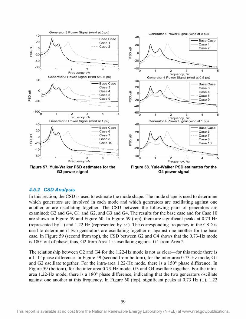
59




4.5.2 CSD Analysis In this section, the CSD is used to estimate the mode shape. The mode shape is used to determine which generators are involved in each mode and which generators are oscillating against one another or are oscillating together. The CSD between the following pairs of generators are examined: G2 and G4, G1 and G2, and G3 and G4. The results for the base case and for Case 10 are shown in Figure 59 and Figure 60. In Figure 59 (top), there are significant peaks at 0.73 Hz (represented by □) and 1.22 Hz (represented by ▽). The corresponding frequency in the CSD is used to determine if two generators are oscillating together or against one another for the base case. In Figure 59 (second from top), the CSD between G2 and G4 shows that the 0.73-Hz mode is 180° out of phase; thus, G2 from Area 1 is oscillating against G4 from Area 2.

The relationship between G2 and G4 for the 1.22-Hz mode is not as clear—for this mode there is a 111° phase difference. In Figure 59 (second from bottom), for the inter-area 0.73-Hz mode, G1 and G2 oscillate together. For the intra-area 1.22-Hz mode, there is a 150° phase difference. In Figure 59 (bottom), for the inter-area 0.73-Hz mode, G3 and G4 oscillate together. For the intra-area 1.22-Hz mode, there is a 180° phase difference, indicating that the two generators oscillate against one another at this frequency. In Figure 60 (top), significant peaks at 0.73 Hz (□), 1.22

0 1 2 3 4 5-60

-40

-20

0

20

40

Frequency, Hz

PS

D, dB



0 1 2 3 4 5-60

-40

-20

0

20

40

Frequency, Hz

PS

D, dB



0 1 2 3 4 5-100

-50

0

50

Frequency, Hz

PS

D, dB



0 1 2 3 4 5-40

-20

0

20

40

Frequency, Hz

PS

D, dB



0 1 2 3 4 5-60

-40

-20

0

20

40

Frequency, Hz

PS

D, dB



0 1 2 3 4 5-40

-20

0

20

40

Frequency, Hz

PS

D, dB



60


Hz (▽), and 1.75 Hz (♢) are visible in the Case 10 example. The 0.73-Hz mode behaves similarly to the previous base case example.

Generators in Area 1 oscillate against the generators in Area 2. When two generators are in the same area, the generators oscillate together for this frequency. Figure 60 (second from top) shows that for the 1.75-Hz mode, the phase-angle shift between G2 and G4 is -160°. Figure 60 (second from bottom) shows that generators G1 and G2 oscillate against one another for the approximately 1.2-Hz mode. For the 1.75-Hz mode, the generators also oscillate against one another. The CSD between G3 and G4 in Figure 60 (bottom) shows that for the 1.22-Hz mode, G3 and G4 are oscillating against one another, and for the 1.75-Hz mode, they are oscillating together. These CSD angle estimates enable the association of modes with areas; for example, the 1.75-Hz mode is associated with Area 1. Changes in inertia in an area will affect these local modes.

0 0.5 1 1.5 2-100

-80

-60

-40

-20

0

20

40

Frequency (Hz)

Magn

itude

(dB)

Base Case

Pout2,Pout4Pout1,Pout2Pout3,Pout4

0 0.5 1 1.5 2-200

0

200

Frequency (Hz)

CSD

Angle

(deg

)

Pout2,Pout4

0 0.5 1 1.5 2-200

0

200

Frequency (Hz)

CSD

Angle

(deg

)

Pout1,Pout2

0 0.5 1 1.5 2-200

0

200

Frequency (Hz)

CSD

Angle

(deg

)

Pout3,Pout4

0 0.5 1 1.5 2-100

-80

-60

-40

-20

0

20

Frequency (Hz)

Magn

itude

(dB)

Case 10

Pout2,Pout4Pout1,Pout2Pout3,Pout4

0 0.5 1 1.5 2-200

0

200

Frequency (Hz)

CSD

Angle

(deg

)

Pout2,Pout4

0 0.5 1 1.5 2-200

0

200

Frequency (Hz)

CSD

Angle

(deg

)

Pout1,Pout2

0 0.5 1 1.5 2-200

0

200

Frequency (Hz)

CSD

Angle

(deg

)

Pout3,Pout4

Figure 59. PSD and CSD angle estimates. □ indicates the 0.73-Hz mode and ▽ indicates

the 1.22-Hz mode.

Figure 60. PSD and CSD angle estimates. □ indicates the 0.73-Hz mode, ▽ indicates the 1.22-Hz mode, and ♢ indicates the 1.75-Hz

mode.

61


4.5.3 Matrix-Pencil Analysis Technique The influence of wind power, location of the WPP, and reduction in inertia on modal damping is examined in this section. The matrix-pencil method is used to estimate the modal frequency and damping in each generator power output for all 11 case studies. Table 7 shows the frequency and damping estimates for G1 and G2 located in Area 1. The inter-area 0.73-Hz mode is seen in the power output for the generators in Area 1, as shown in Table 7. As shown earlier in this section, the 0.73-Hz mode shifts to approximately 0.77 Hz when the inertia is reduced in either Area 1 or Area 2. The damping estimates for Cases 1 to 10 indicate that the 0.77-Hz mode is better damped for cases when the inertia is reduced in Area 1 or in Area 2 and is not dependent on wind power penetration or on WPP location.

Table 8 shows the estimated modal frequencies and damping for G3 located in Area 2. A 1.22-Hz mode is seen in the power output of G3 in addition to the inter-area 0.73-Hz mode. As shown earlier in this section, when the inertia in Area 1 in reduced, the 1.22-Hz frequency shifts to 1.78 Hz. The damping for the 0.73-Hz mode is improved when the inertia is reduced in Area 1 or in Area 2 and is not dependent on wind power penetration or on WPP location. The damping for the 1.22-Hz mode is not altered by wind power penetration, location of the WPP, or by the reduction of inertia. Similar results are seen for the estimated modal frequencies and damping for G4 located in Area 2 and are given in Table 9.

Table 7. Area 1 Frequency and Damping Estimates for the 0.73-Hz Mode

G1 G2 Case No.

Freq (Hz)

Damping (%)

Freq (Hz)

Damping (%)

Base 0.73 0.07 0.73 0.06 1 0.78 0.29 0.78 0.28 2 0.77 0.41 0.77 0.61 3 0.78 0.39 0.78 0.36 4 0.78 0.38 0.78 0.37 5 0.77 0.48 0.77 0.63 6 0.77 0.47 0.78 0.47 7 0.77 0.53 0.77 0.58 8 0.76 0.54 0.76 0.64 9 0.77 0.46 0.78 0.57 10 0.77 0.61 0.77 0.65

62


4.5.4 Modes with Additional WPP Controls The additional controls added to the WPP to improve frequency response perform as expected, as shown by the system average frequency response plot in Figure 61. The case with both droop and inertia enabled performs best in terms of frequency response.

Table 8. Area 2 G3 Frequency and Damping Estimates for the 0.73-Hz and 1.22-Hz Modes

0.73-Hz Mode 1.22-Hz Mode Case No.

Freq (Hz)

Damping (%)

Freq (Hz)

Damping (%)

Base 0.73 0.08 1.22 4.35 1 0.78 0.28 1.78 3.97 2 0.78 0.37 1.22 4.24 3 0.78 0.44 1.78 4.64 4 0.78 0.41 1.78 4.19 5 0.77 0.51 1.22 4.26 6 0.78 0.51 1.77 4.54 7 0.77 0.57 1.77 4.63 8 0.76 0.57 1.21 4.50 9 0.78 0.48 1.19 5.07 10 0.77 0.63 1.21 4.60

Table 9. Area 2 G4 Frequency and Damping Estimates for the 0.73-Hz and 1.22-Hz Modes

0.73-Hz Mode 1.22-Hz Mode Case No.

Freq (Hz)

Damping (%)

Freq (Hz)

Damping (%)

Base 0.73 0.06 1.22 4.36 1 0.78 0.12 1.79 3.89 2 0.78 0.32 1.22 4.35 3 0.78 0.50 1.78 4.42 4 0.78 0.35 1.79 3.99 5 0.77 0.51 1.22 4.52 6 0.78 0.50 1.78 4.43 7 0.77 0.59 1.78 4.45 8 0.76 0.57 1.21 4.79 9 0.78 0.52 1.22 4.72 10 0.77 0.63 1.21 4.87

63


Figure 61. Frequency response plots with additional WPP controls

Table 10 and Table 11 list the frequency and damping of each mode observed for each of the cases. In terms of modal behavior, there is no significant difference between any of the cases shown here. Thus, it can be inferred that these controls do not have significant impact on modal behavior. More aggressive droop curves and control modifications will be studied in future work to determine if these controls may affect modal behavior.

80 90 100 11059.88

59.9

59.92

59.94

59.96

59.98

60

60.02

60.04

Time (sec)

Freq

uenc

y (H

z)

BaseDroop+InertiaDroopInertia

Table 10. Area 1 Frequency and Damping Estimates

G1 G2

Case Freq (Hz)

Damping (%)

Freq (Hz)

Damping (%)

Base Case

- - 1.76 5.90 0.78 0.37 0.78 0.53

Droop - - 1.76 5.71 0.78 0.52 0.77 1.14

Inertia - - 1.76 5.74 0.77 0.68 0.76 1.04

Droop + Inertia

1.74 5.52 1.75 5.63 0.77 0.76 0.76 1.14

64


4.6 Summary The work discussed here indicates that the displacement of inertia because of WPP integration results in changes in the frequency and damping of oscillation modes. The location of inertia displacement in the system is also of importance. Frequency response controls or WPP output levels do not appear to influence these modes (note, however, that this might not be the case in a highly congested system). The benefit of the analysis technique described in this chapter is that network data need not be known. In future work, these results will be validated using archived PMU data from real power systems correlated with information about WPP installations and CPP retirements and system planners could conduct similar analyses to evaluate system stability. As the wind penetration level increases, such analyses will become increasingly relevant.

4.7 References [1] DOE. 20% Wind Energy by 2030: Increasing Wind Energy’s Contribution to U.S.

Electricity Supply. NREL/TP-500-41869, DOE/GO-102008-2567. Golden, CO: May 2008. Accessed November 2013: www.nrel.gov/docs/fy08osti/41869.pdf.

[2] Electric Reliability Council of Texas. “ERCOT Grid Operations Wind Integration Report: 05/02/2013.” 2013. Accessed November 2013: www.ercot.com/content/gridinfo/generation/windintegration/2013/05/ERCOT%20Wind%20Integration%20Report%2005-02-13.pdf.

[3] GE Energy. Western Wind and Solar Integration Study. Golden, CO: National Renewable Energy Laboratory, 2010. NREL/SR-550-47434. Accessed November 2013: www.nrel.gov/docs/fy10osti/47434.pdf.

[4] Miller, N.; Shao, M.; Venkataraman, S. CAISO Frequency Response Study. Schenectady, New York: GE Energy, 2011. Accessed November 2013: www.uwig.org/Report-FrequencyResponseStudy.pdf.

[5] Slootweg, J.G.; Kling, W.L. “The Impact of Large-Scale Wind Power Generation on Power System Oscillations.” Electric Power Systems Resources (67), 2003; pp.9–20.

Table 11. Area 1 Frequency and Damping Estimates

G1 G2

Case Freq (Hz)

Damping (%)

Freq (Hz)

Damping (%)

Base Case

- - 1.76 5.90 0.78 0.37 0.78 0.53

Droop - - 1.76 5.71 0.78 0.52 0.77 1.14

Inertia - - 1.76 5.74 0.77 0.68 0.76 1.04

Droop + Inertia

1.74 5.52 1.75 5.63 0.77 0.76 0.76 1.14

http://www.nrel.gov/docs/fy08osti/41869.pdf

http://www.ercot.com/content/gridinfo/generation/windintegration/2013/05/ERCOT%20Wind%20Integration%20Report%2005-02-13.pdf

http://www.ercot.com/content/gridinfo/generation/windintegration/2013/05/ERCOT%20Wind%20Integration%20Report%2005-02-13.pdf


http://www.uwig.org/Report-FrequencyResponseStudy.pdf

http://www.uwig.org/Report-FrequencyResponseStudy.pdf

65


[6] Tsourakis, G.; Nomikos, B.M.; Vournas, C.D. “Contribution of Doubly-Fed Wind Generators to Oscillation Damping.” IEEE Transactions on Energy Conversion (24:3), Sept. 2009; pp.783–791.

[7] Mendonca, A.; Peas Lopes, J.A. “Impact of Large-Scale Wind Power Integration on Small Signal Stability.” 2005 International Conference on Future Power Systems Proceedings; Nov. 2005.

[8] Gautam, D.; Vittal,V.; Harbour, T. “Impact of Increased Penetration of DFIG-Based Wind Turbine Generators on Transient and Small-Signal Stability of Power Systems.” IEEE Transactions on Power Systems (24:3), Aug. 2009; pp.1426–1434.

[9] Kundur, P. Power System Stability and Control. New York: McGraw Hill, 1974; pp. 814.

[10] Manitoba HVDC Research Centre. PSCAD/EMTDC: Electromagnetic Transients Program Including DC Systems. Winnipeg, Manitoba, 1994.

[11] Das, T.K.; Venayagamoorthy, G.K. “Optimal Design of Power System Stabilizers Using a Small Population-Based PSO.” Preprint. Prepared for the IEEE Power Engineering Society General Meeting, June 12–16, 2006, Montreal, Quebec.

[12] Behnke, M.; Ellis, A.; Kazachkov, Y.; McCoy, T.; Muljadi, E.; Price, W.; Sanchez-Gasca, J. “Development and Validation of WECC Variable Speed Wind Turbine Dynamic Models for Grid Integration Studies.” 2007 WindPower Conference Proceedings; June 2007, Los Angeles, California.

[13] Singh, M.; Santoso, S. Dynamic Models for Wind Turbines and Wind Power Plants. NREL/SR-5500-52780. Golden, CO: National Renewable Energy Laboratory, 2011. Accessed November 2013: www.nrel.gov/docs/fy12osti/52780.pdf.

[14] Pierre, J.W.; Trudnowski, D.J.; Donnelly, M.K. “Initial Results in Electromechanical Mode Identification from Ambient Data.” IEEE Transactions on Power Systems (12:3), 1997; pp. 1245–1251.

[15] WECC Modeling and Validation Work Group, Renewable Energy Modeling Task Force. WECC Wind Power Plant Dynamic Modeling Guide. November 2010. Accessed November 2013: http://renew-ne.org/wp-content/uploads/2012/05/WECCWindPlantDynamicModelingGuide.pdf.

[16] Muljadi, E.; Butterfield, C.P.; Ellis, A.; Mechenbier, J.; Hocheimer, J.; Young, R.; Miller, N.; Delmerico, R.; Zavadil, R.; Smith, J.C. “Equivalencing the Collector System of a Large Wind Power Plant.” Preprint. Prepared for the IEEE Power Engineering SocietyGeneral Meeting, June 12–16, 2006, Montreal, Quebec.

[17] Lalor, G.; Mullane, A.; O’Malley, M. “Frequency Control and Wind Turbine Technologies.” IEEE Transactions on Power Systems (20:4), 2005; pp.1,905–1,913.


http://renew-ne.org/wp-content/uploads/2012/05/WECCWindPlantDynamicModelingGuide.pdf

http://renew-ne.org/wp-content/uploads/2012/05/WECCWindPlantDynamicModelingGuide.pdf

66


[18] Ramtharan, G.; Ekanayake, J.B.; Jenkins, N. “Frequency Support from Doubly-Fed Induction Generator Wind Turbines.” IET Renewable Power Generation (1), 2007; pp.3–9.

[19] Conroy, J.F.; Watson, R. “Frequency Response Capability of Full-Converter Wind Turbine Generators in Comparison to Conventional Generation.” IEEE Transactions on Power Systems (23:2), May 2008; pp.649–656.

[20] Ullah, N.R.; Thiringer, T.; Karlsson, D. “Temporary Primary Frequency Control Support by Variable-Speed Wind Turbines—Potential and Applications.” IEEE Transactions on Power Systems (23:2), 2008; pp. 601–612.

[21] Buckspan, A.; Aho, J.; Fleming, P.; Jeong, Y.; Pao, L. “Combining Droop Curve Concepts with Control Systems for Wind Turbine Active Power Control.” Preprint. Prepared for the IEEE Power Electronics and Machines in Wind Applications, July 2012, Denver, Colorado.

[22] Morren, J.; De Haan, S.W.H.; Kling, W.L.; Ferreira, J.A. “Wind Turbines Emulating Inertia and Supporting Primary Frequency Control.” IEEE Transactions on Power Systems (21:1), Feb. 2006; pp. 433–434.

[23] Kamwa, A.; Pradhan, A.K.; Joos, G. “Adaptive Phasor and Frequency-Tracking Schemes for Wide-Area Protection and Control.” IEEE Transactions on Power Delivery (26:2), April 2011; pp. 744–753.

[24] Sarkar, T.K.; Pereira, O. “Using the Matrix Pencil Method to Estimate the Parameters of a Sum of Complex Exponentials.” IEEE Antennas and Propagation Magazine (37:1), 1995; pp. 48–55.

[25] Bounou, M.; Lefebvres, S.; Malhame, R.P. “A Spectral Algorithm for Extracting Power System Modes from Time Recordings.” IEEE Transactions on Power Systems (7:2), 1992; pp. 665–672.

[26] Welch, P.D. “The Use of Fast Fourier Transform for the Estimation of Power Spectra: A Method Based on Time Averaging Over Short, Modified Periodograms.” IEEE Transactions on Audio and Electroacoustics (15:2), June 1967; pp.70–73.

[27] Zhou, N.; Trudnowski, D.; Pierre, J.W.; Sarawgi, S.; Bhatt, N. “An Algorithm for Removing Trends from Power-System Oscillation Data.” Preprint. Prepared for the 2008 IEEE Power and Energy Society General Meeting – Conversion and Delivery of Electrical Energy in the 21st Century, July 2008, Pittsburgh, Pennsylvania.

[28] Andersson, G.; Atmuri, R.; Rosenqvist, R.; Torseng, S. “Influence of Hydro Units’ Generator-to-Turbine Inertia Ratio on Damping of Subsynchronous Oscillations.” IEEE Transactions on Power Apparatus and Systems (103:8), Aug. 1984; pp. 2,352–2,361.

[29] Klein, M.; Rogers, G.J.; Kundur, P. “A Fundamental Study of Inter-Area Oscillations in Power Systems.” IEEE Transactions on Power Systems (6:3), Aug. 1991; pp. 914–921.

synchrophasor applications for wind power generation · mpp maximum power point . mppt maximum...

Documents