synchrophasor-based backup differential protection...
TRANSCRIPT

______________________________________________________________________________
Synchrophasor-Based Backup Differential Protection Design
of Transmission Lines _____________________________________________________________________________________
Prepared by Yaojie Cai Keke Jin
Grace Ngantian Jiajing Wang
Final Report submitted in partial satisfaction of the requirements for the degree of Bachelor of Science
in Electrical and Computer Engineering
in Faculty of Engineering
of the University of Manitoba
Faculty Supervisor: Dr. Athula Rajapakse
Spring 2014
© Copyright by Yaojie Cai, Keke Jin, Grace Ngantian, and Jiajing Wang, 2014

ii
Abstract When power system disturbances occur, they can lead to large scale power outages if these disturbances
are ignored and no action is taken to clear them. In the past few years, many blackouts have happened as a
result of poor fault detection methods implemented over a wide area. With the objective of improving
these methods, this report describes the design and development of a synchrophasor-based backup
differential protection system using transmission line monitoring to detect faults.
For experimental purposes, the power system portion of the proposed synchrophasor network is simulated
using a real-time digital simulator (RTDS). The RTDS generates analog current and voltage outputs
corresponding to the designed power system in real time, and they are used as inputs to phasor
measurement units (PMUs). These units take phasor measurements of the simulated transmission line at
different locations synchronously through the use of a Global Positioning System (GPS) clock—thus, the
measurements are referred to as synchrophasors. The synchrophasor data is then used to detect faults by
applying a detection algorithm to the data, which will also pinpoint the location of the fault along the line.
If a fault is detected, a backup signal produced by a microcontroller will be sent to trip the breakers in
order to isolate the fault.
To test the design, the RTDS was used to simulate various types of faults. The test results verify that the
designed synchrophasor-based protection system is highly accurate and reliable. Therefore, it is
applicable to modern power systems.

iii
Contributions The advancement of Synchrophasor-based Protection will contribute to wide area monitoring of
transmission line. This project can be divided into four parts:
1. Model building and Hardware Configuration
2. Developing Fault Detection Algorithm and Window Application
3. Designing and Implementation Fault Locator Algorithm
4. Designing the Backup Protection Implementation
Dr. A. Rajapakse is our faculty advisor. The project was conceived by him. He provided valuable
experience, knowledge and guidance to us throughout the project.
Rubens Eduardo Almiron Bonnin, Naushath Monhamed Haleem, and Dinesh Gurusinghe provided us
with help and valuable advice regarding academic theory.
Grace was responsible for implementing a power system model in RTDS simulator with analog outputs
suitable to interface with PMUs.
Yaojie was responsible for implementing a differential protection algorithm for fault detection and
develop a window application for displaying fault-condition results.
Keke Jin was responsible for testing and implementing Phasor-based Method to pinpoint the location of
fault in transmission line.
Jiajing was responsible for designing a method for utilizing microcontroller to send alarm signal for
indicating fault through an IP network.

iv
Acknowledgments
It is with immense gratitude that we acknowledge the support and help of our Professor Athula Rajapakse.
It was an honour to receive advice from such a knowledgeable person.
We must also thank Rubens Eduardo Almiron Bonnin, Naushath Monhamed Haleem, Dinesh Gurusinghe
and other academic, technical staff in the power research group. Without their guidance and persistent
help this project would not have been possible.
We would like to thank our examining committee for spending the time to review our thesis.
Yaojie Cai
Keke Jin
Grace Ngantian
Jiajing Wang

v
Nomenclature Abbreviations RTDS: Real Time Digital Simulator
PMU: Phasor Measurement Unit
GPS: Global Positioning System
PDC: Phasor Data Concentrator
SEL: Schweitzer Engineering Laboratories
CT: Current Transformer
PT: Potential Transformer
CVT: Capacitive Voltage Transformer
GTAO: Giga Transceiver Analog Output
GPC: Giga-Processor Card
TCP/IP: Transmission Control Protocol / Internet Protocol
UDP: User Datagram Protocol
LED: Light-Emitting Diode
Symbols
: Total current of Phase A from vector summation of both ends of Transmission line.
: Total current of Phase B from vector summation of both ends of Transmission line.
: Total current of Phase C from vector summation of both ends of Transmission line.
: Phase A current from sending end of Transmission line.
: Phase B current from sending end of Transmission line.
: Phase C current from sending end of Transmission line.
: Phase A current from receiving end of Transmission line.
: Phase B current from receiving end of Transmission line.
: Phase C current from receiving end of Transmission line.
: Total current between Phase A and C from vector summation of both ends of Transmission line.
: Total current between Phase B and C from vector summation of both ends of Transmission line.
: Total current between Phase C and A from vector summation of both ends of Transmission line.
A complex number which has 1 amplitude and phase is 120 degree ∠ .
: Total zero sequence current from vector summation of both ends of Transmission line.

vi
: Total positive sequence current from vector summation of both ends of Transmission line.
: Total negative sequence current from vector summation of both ends of Transmission line.
∠ : The angle of total zero sequence current.
∠ : The angle of total negative sequence current.
| | The magnitude of total current between Phase B and C.
: The maximum number among A, B and C.
K: Restraint coefficient
a: Assumed magnitude of phase current from sending end of transmission line.
b: Assumed phase difference of phase current between sending end and receiving end of transmission line.
: Estimated distance to the fault location.
dexact :Exact distance to the fault location.
: Total line length of transmission line.
X: Distance to fault location from receiving end of transmission line.
Voltage at fault location.
: post fault voltages at sending
: post fault voltages at receiving end
: Post fault currents at sending ends
Post current receiving ends
: Characteristic impedance;
γ: Propagation constant.
Coefficients of differential equation of voltage in Long Line Transmission Model.

vii
List of Figures
Figure 1.1: Main Setup
Figure 2.1: Preliminary Power System Model in RSCAD
Figure 2.2: Secondary Power System Model in RSCAD
Figure 2.3: Secondary Model in PSS/E
Figure 2.4: Current and Voltage Inputs of the SEL-421
Figure 2.5: GTAO Card
Figure 2.6: RTDS/PMU Interface
Figure 3.1: False Warning Window under Phase A and B Line to Ground Fault
Figure 3.2: Current vs Package Index Plot under Phase A and B Line to Ground Fault
Figure 3.3: Detecting Fault Time for Current Magnitude Threshold and Phase Selection Method
Figure 3.4: Detecting Fault Time for Current Scalar Summation Method
Figure 4.1: Transmission Long Line Model
Figure 4.2: Unsaturation Case of Estimated Current (IAs) vs Actual Current (IBRKA2)
Figure 4.3: Post Fault Voltage Curve
Figure 4.4: Post Fault Current Curve
Figure 4.5: Real Parts of Voltage Phase A on the Sending End of Transmission Line
Figure 4.6: Imaginary Parts of Voltage Phase A on the Sending End of Transmission Line
Figure 4.7: Flowchart of Matlab program for calculating the Fault location
Figure 4.8 3: Phase Fault -Measured Error percentage vs Actual Fault location
Figure 4.9: LG Fault -Measured Error percentage vs Actual Fault location
Figure 4.10: LLG Fault -Measured Error percentage vs Actual Fault location

viii
Figure 4.11: Various Fault Impendence -Measured Error percentage vs Actual Fault location
Figure 5.1: SEL-421 Functional Overview
Figure 5.2: Original Breaker Logic Circuit
Figure 5.3: A Complete Program for the Microcontroller Interface method
Figure 5.4: Program for the LED Demonstration
Figure 5.5: Program for Input Signal Checking in Raspberry Pi
Figure 6.1: Icon
Figure 6.2: Parent Window
Figure 6.3: Overall Structure of the Fault-monitoring Program
Figure 6.4: "Connection" Tab
Figure 6.5: Monitoring Window.
Figure 6.6: Flow Chart for the Fault Detector and Fault Locator
Figure 6.7: Fault Location Calculator
Figure 6.8: Warning Window
Figure 6.9: Screenshot of the Visual Studio 2012 IDE
Figure 6.10: Plot of Data Package 285 during Fault Condition
Figure 6.11: Phasor Diagram from the Monitor Window during the Fault Condition
Figure 6.12: Interface for the Transmission Line Database
Figure 6.13: Line to Line and Line to Ground Fault in the Simulation Model

ix
List of Tables
Table 1.1: Specifications
Table 4.1: Characteristics of Impedance-based Method and Phasor-based Method
Table 5.1: Microcontroller Comparison
Table 6.1: Result from the Fault-monitoring Program during Phase A and B Line to Line Fault
Table 6.2: Result from the Fault-monitoring Program during Phase B and C Line to Line Fault
Table 6.3: Result from the Fault-monitoring Program during Phase A and C Line to Line Fault
Table 6.4: Result from the Fault-monitoring Program during Phase A, B and C Line to Line Fault
Table 6.5: Result from the Fault-monitoring Program during Phase A Line to Ground Fault
Table 6.6: Result from the Fault-monitoring Program during Phase B Line to Ground Fault
Table 6.7: Result from the Fault-monitoring Program during Phase C Line to Ground Fault
Table 6.8: Result from the Fault-monitoring Program during Phase A and B Line to Ground Fault
Table 6.9: Result from the Fault-monitoring Program during Phase A and B Line to Ground Fault
Table 6.10: Result from the Fault-monitoring Program during Phase A and C Line to Ground Fault
Table 6.11: Result from the Fault-monitoring Program during three Phases to Ground Fault

x
Table of Contents
Abstract ........................................................................................................................................................ ii
Contributions.............................................................................................................................................. iii
Acknowledgements .................................................................................................................................... iv
Nomenclature ............................................................................................................................................. v
List of Figures ............................................................................................................................................ vii
List of Tables .............................................................................................................................................. ix
Table of Contents ........................................................................................................................................ x
Chapter 1 Introduction ............................................................................................................................... 1
1.1 Motivation ........................................................................................................................................... 1
1.2 Project Overview................................................................................................................................. 1
1.3 Specifications ...................................................................................................................................... 3
Chapter 2 Power System Model and Hardware Configuration ............................................................. 4
2.1 Introduction ......................................................................................................................................... 4
2.2 Power System Expansion .................................................................................................................... 4
2.2.1 Load Flow Analysis ..................................................................................................................... 6
2.2.2 Power System Simulation ............................................................................................................ 7
2.3 Synchrophasor Network ...................................................................................................................... 7
2.3.1 Hardware PMU Configuration ..................................................................................................... 7
2.3.2 Current and Voltage Inputs .......................................................................................................... 8
2.4 RTDS/PMU Interface ......................................................................................................................... 8
2.4.1 Analog Output Scaling ............................................................................................................... 10
2.4.2 Synchrophasor Data Transmission ............................................................................................. 10
2.5 Chapter Summary ............................................................................................................................. 10
Chapter 3 Fault Detection Algorithm ..................................................................................................... 12
3.1 Introduction ....................................................................................................................................... 12
3.2 Algorithms ........................................................................................................................................ 12
3.2.1 Current Magnitude Threshold and Phase Selection Method ...................................................... 12
3.2.2 Current Scalar Summation and Vector Summation Comparison Method ................................. 16
3.2.3 Test Result and Recommendations ............................................................................................ 17
3.3 Chapter Summary ............................................................................................................................. 19

xi
Chapter 4 Fault Location Algorithm ...................................................................................................... 20
4.1 Introduction ....................................................................................................................................... 20
4.2 Accuracy of Fault Location ............................................................................................................... 21
4.3 Phasor-based Method vs. Impedance-based Method ........................................................................ 22
4.4 Principle of Phasor-based Method .................................................................................................... 24
4.5 Experiment Process ........................................................................................................................... 26
4.5.1 RSCAD PMU Model and CT Saturation Test ........................................................................... 27
4.5.2 Post Fault Condition Measurement ............................................................................................ 28
4.5.3 Fault Location Calculation ......................................................................................................... 29
4.6 Estimated Result and Analysis .......................................................................................................... 32
4.6.1 Various Fault Types ................................................................................................................... 33
4.6.2 Various Fault Impedances .......................................................................................................... 35
4.7 Chapter Summary ............................................................................................................................. 36
Chapter 5 Backup Protection Implementation ...................................................................................... 37
5.1 Introduction ....................................................................................................................................... 37
5.1.1 Background ................................................................................................................................ 37
5.1.2 Purpose ....................................................................................................................................... 39
5.2 Methods ............................................................................................................................................. 39
5.2.1 Alternative Logic Circuit ........................................................................................................... 39
5.2.2 Microcontroller Interface ........................................................................................................... 41
5.2.3 Selection of Method ................................................................................................................... 42
5.3 Implementation ................................................................................................................................. 42
5.3.1 Microcontroller Selection .......................................................................................................... 43
5.3.2 Scheme and Procedure ............................................................................................................... 44
5.3.3 Result ......................................................................................................................................... 46
5.4 Further Improvement ........................................................................................................................ 46
5.5 Chapter Summary ............................................................................................................................. 47
Chapter 6 Windows Application ............................................................................................................. 48
6.1 Introduction ....................................................................................................................................... 48
6.2 Structure of the Program ................................................................................................................... 49
6.2.1 Fault Detector ............................................................................................................................. 52
6.2.2 Fault Location Calculator........................................................................................................... 53

xii
6.2.3 Fault Alarm Message ................................................................................................................. 54
6.2.4 Graphic User Interface, Plot and Database ................................................................................ 54
6.3 Estimated Results .............................................................................................................................. 57
6.3.1 Line to Line Fault ....................................................................................................................... 57
6.3.2 Line to Ground Fault .................................................................................................................. 59
6.3.3 Three Phases to Ground Fault .................................................................................................... 61
6.4 Future Work ...................................................................................................................................... 61
6.5 Chapter Summary ............................................................................................................................. 62
Chapter 7 Conclusion ............................................................................................................................... 63
References .................................................................................................................................................. 64
Vita ............................................................................................................................................................. 65
Yaojie,Cai .................................................................................................................................................. 66
KeKe, Jin ................................................................................................................................................... 67
Grace,Ngantian .......................................................................................................................................... 68
Jiajing,Wang ............................................................................................................................................... 69
Appendix A ............................................................................................................................................... 70
Appendix B ............................................................................................................................................... 72
Appendix C ............................................................................................................................................... 74
Appendix D ............................................................................................................................................... 76
Appendix E ............................................................................................................................................... 76

1
Chapter 1 Introduction
This chapter contains the motivation for this project, as well as the project overview,
followed by the design specifications.
1.1 Motivation
Currently, there is a high demand for electrical energy and it is therefore crucial to
consider reliability in power systems. Protection systems play an important role in reliability, as
they are used to maintain power system stability if any faults occur. These protection systems are
used to detect faults when they occur, and then immediately isolate the faults in order to minimize
grid damage and prevent power outages.
There are various methods of fault detection, but this project focuses on wide area
monitoring, which is a very useful tool in protection of large transmission lines. The main cause
of large blackouts today is the implementation of poor line monitoring methods that are unable to
observe the state of a power system over a wide area. As a result, various instabilities in the
network can have a cascade effect over a large distance if they are not detected and no actions are
taken to control them.
The main objective is to design a differential protection algorithm using synchronized
phasor measurements obtained from two ends of a transmission line, and to implement it on real
time hardware for testing. The motivation of this project is to detect various types of faults and to
determine the fault location on a transmission line, while considering both speed and accuracy
optimization.
1.2 Project Overview
The main components of this project and the connections between them are shown in
Figure 1.1 below. They include: two phasor-measurement units (PMUs) which monitor two ends
of a transmission line, as well as a phasor data concentrator (PDC) which will collect
synchrophasor data from the PMUs and then send the data to an endpoint computer for fault
analysis. These data transmissions will occur through Ethernet. A windows application will be
developed to display the synchrophasor measurements and it will also alert the user when a fault
occurs. Note that the power system outputs are simulated using the RTDS unit.

2
Figure 1.1: Main Setup

3
1.1 Specifications
Table 1.1: Specifications Specification of Self-developed Window Application
Specifications
Operating System Microsoft Windows
Method of Communication Client-server
Data Transmission Rate 60 Frames per second
Protocol Standard IEEE Standard for Sychrophasor Data Transfer
Stability1 >99.9%
Reliability2 >99.9%
Fault Location Error 3 <5%
1 The probability of Self-developed Window Application not to crash during
monitoring process. 2 The probability of Fault Detection function in Self-developed Window Application
is not to be triggered by external faults. 3 Error of result of Fault Locator in Self-developed Window Application

4
Chapter 2 Power System Model and Hardware Configuration
2.1 Introduction
The design of the power system model for this project was done with the intent of testing
a very simple system for demonstration purposes, since an intricate system was unnecessary. Also,
we can expect similar results for large scale networks because the spacing of the PMUs along the
line will approximately be the same.
The hardware configurations of the PMUs and RTDS play a large role in this project,
since the simulation of a power system must be done with minimal errors in order to generate
proper analog outputs that we would expect from a real system. Moreover, the results of the fault
analysis algorithms heavily rely on the accuracy of the synchrophasor measurements taken by the
hardware PMUs.
2.2 Power System Expansion
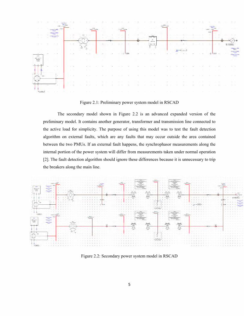
The preliminary power system model is shown in Figure 2.1. It includes a generator, a
transformer, one 210 kV and 207 km transmission line, along with an active load. The generator
side will be referred to as Station A, and the active load side will be referred to as Station B. Also,
two PMUs are connected at both ends of the transmission line to provide phasor measurements of
voltage and current at each station. All of the parameters for the generator, transmission line,
transformer were taken from a reliable source to mimic a real case scenario, and are shown in
Appendix A [1]. Similarly, the parameters for the instrument transformers can be found in
Appendix B.
5
Figure 2.1: Preliminary power system model in RSCAD
The secondary model shown in Figure 2.2 is an advanced expanded version of the
preliminary model. It contains another generator, transformer and transmission line connected to
the active load for simplicity. The purpose of using this model was to test the fault detection
algorithm on external faults, which are any faults that may occur outside the area contained
between the two PMUs. If an external fault happens, the synchrophasor measurements along the
internal portion of the power system will differ from measurements taken under normal operation
[2]. The fault detection algorithm should ignore these differences because it is unnecessary to trip
the breakers along the main line.
Figure 2.2: Secondary power system model in RSCAD

6
2.2.1 Load Flow Analysis
Before simulating the power system, it was necessary to perform a load flow analysis on
the proposed design to ensure that there were no errors that may interfere with the experimental
results. This was done using PSS/E software, which is commonly used to analyze power system
performances. Figure 2.3 shows the drafted secondary model in PSS/E under a load flow analysis.
The green arrows show the direction of real power while the orange arrows show the direction of
reactive power. Clearly, the model feasible since there are no problems with the load flows—
power is being supplied by the generators and absorbed by the load.
Figure 2.3: Secondary Model in PSS/E

7
2.2.2 Power System Simulation
The designed power systems were simulated using RSCAD which is compatible with the
RTDS. Once the RSCAD model has been compiled, it will allow the RTDS to generate analog
outputs in real time that are suitable for the PMUs [3]. These analog outputs include the voltage
and current outputs of potential and current transformers along the sending and receiving ends of
the transmission line.
2.3 Synchrophasor Network
The SEL-421 is a Schweitzer Engineering Laboratories (SEL) relay device that has a
wide variety of functions pertaining to protection, automation and controls. Specifically for this
project, two of these relays are used as PMUs. They can obtain highly accurate synchrophasor
measurements when a GPS clock is connected to these devices. The GPS clock will ensure that
the voltage and current measurements taken by both PMUs are synchronized. It is crucial that the
measurements are taken at exactly the same time because any time delay between these
measurements can impact the results in such a way that a fault may be falsely detected; the
algorithm will only be effective when measurements are fully synchronized.
2.3.1 Hardware PMU Configuration
In order to configure the PMUs, there are many parameters that must be set in order to
achieve accurate results in synchrophasor measurements. These include global settings,
transmission line parameters, and line configuration parameters. The AcSELerator Quickset
software developed by Schweitzer Engineering Laboratories Inc. was used to configure these
settings.
Firstly, the global settings are shown in Appendix C.1 and they are used to set up the
main parameters such as location and nominal frequency, while also being used to enable the
synchrophasor measurement function.
Appendix C.2 displays the transmission line parameters for the transmission line
simulated in RSCAD. The positive and zero sequence impedances for the transmission line must
be specified to accurately determine the voltage and current values at the sending end and
receiving end of the line.

8
The relay impedance settings as shown in Appendix C.3 are specified in secondary ohms.
These settings are used to find the reach settings of the phase and ground distance elements, and
were calculated considering the CT and PT ratios. These calculations are then used to determine
the line configuration parameters, which are found in Appendix C.4.
2.3.2 Current and Voltage Inputs
The PMUs are designed to receive current and voltage signals in analog form, as they are
connected to Current Transformers (CTs) and Potential Transformers (PTs) that step down the
AC currents and voltages of the transmission line in practice. These current and voltage inputs are
shown in Figure 2.4. The nominal current ratings are 1 A or 5 A while the nominal voltage ratings
are 69 V.
Figure 2.4: Current and Voltage Inputs of the SEL-421
The SEL-421 also has the capability of receiving inputs through a low-level analog
interface. This interface is typically used for testing in laboratories when the analog signals are
simulated, since the ratings are quite low. The nominal current rating is 67 mA while the nominal
voltage rating is 446 mV.
2.4 RTDS/PMU Interface
Since the PMUs require analog inputs, the digital outputs of the RTDS corresponding to
the simulated power system model in RSCAD must be converted to analog form. Therefore, an
analog output card was needed to perform the conversion before connecting to the PMUs [4]. The
card provided with the RTDS is called a Gigabit Tranceiver Analog Output (GTAO) card as
shown in Figure 2.6. The GTAO card is interfaced with the Giga-Processor Card (GPC), which
Current Inputs Voltage Inputs

9
solves equations related to the power system in RSCAD in order to simulate the current and
voltage outputs.
Since the analog outputs of the GTAO card are significantly lower than the outputs of
CTs and PTs, these outputs must be amplified before connecting to the PMUs using voltage and
current amplifiers [5]. Thus, the gains of the amplifiers can be calculated by using the ratios
between the instrument transformer outputs and the GTAO outputs. However, as previously
mentioned, the SEL-421 has a low-level interface that accepts analog outputs with lower
amplitudes than instrument transformer outputs. Therefore, this project did not require the use of
amplifiers.
Figure 2.6: GTAO card
The basic interface between the RTDS and the PMUs is shown in Figure 2.7. Once the
CTs, PTs and CVTs were modeled and compiled in RSCAD, the RTDS will generate the required
digital outputs which will then be processed by the GTAO card. Note that the instrument
transformer turn ratios were determined by considering the ratio between the current and voltage
ratings required by the PMUs and the current and voltage ratings of the transmission line.
Figure 2.7: RTDS/PMU Interface
Instrument Transformers
(CTs, PTs, & CVTs)
GTAO Card
PMUs (SEL-421)
Digital
Analog

10
2.4.1 Analog Output Scaling
The GTAO card must be configured to generate the correct analog signal levels before
directly connecting to the low-level interface of the SEL-421 relays. This is done by setting the
scaling factor for the card in RSCAD. The equation (2.1) below was extracted from the RTDS
manual [1] and it is used to calculate the scaling factors shown in (2.2) and (2.3).
(2.1)
Current scaling factor calculation:
(2.2)
Voltage scaling factor calculation:
(2.3)
2.4.2 Synchrophasor Data Transmission
The SEL-421 relays measure the phasor values at both ends of the transmission line
synchronously, and will then transmit the synchrophasor data to the PDC, which collects and
packages the data. The AcSELerator Quickset software was used to configure the
communications for the relays. This allows the user to set up the serial port and Ethernet port
parameters. For this project, the synchrophasor data transmission occurs via Transmission
Communication Protocol/ Internet Protocol (TCP)/ (IP), although User Datagram Protocol (UDP)
is another option. All of the communication configurations are shown in Appendix D.
2.5 Chapter Summary
To summarize the hardware portion of the project related to the generation and
measurement of synchrophasors, once the power system model was designed and drafted in
RSCAD, the RTDS unit collects the model data to produce current and voltage outputs in digital
form. The GTAO card is used to convert the digital signals to analog outputs suitable for the low-

11
level interface of the PMUs. Afterwards, the PMUs are configured to send the synchrophasor data
to the PDC through a TCP network. The PDC will then send the compressed data to an endpoint
computer for fault analysis, which is discussed in the next two chapters.

12
Chapter 3
Fault Detection Algorithm
3.1 Introduction
The fault detection algorithm is based on the Current Differential Protection Method. In the
normal condition, a three-phase power system is balanced which means the magnitudes of the
currents of all three phases (phases A, B and C) are identical and each phase is separated by a
phase angle of 120°. During a fault, the transmission system becomes unbalanced, both
magnitudes and phase angles of the currents will be changed. By recognizing the changes in the
phase currents, the fault itself and the type of it can be detected.
3.2 Algorithms
The fault conditions are detected by monitoring the phase impedances, phase-current
amplitudes, phase-voltage amplitudes and zero-sequence current amplitudes. The general
structure of the fault-detection algorithm is to utilize two different statistic measurements of the
voltage or current signals, which are determined with the voltmeter and ampere meter. The
criterion value is formulated to assess the fault inception. Based on the Kirchhoff's Current Law,
the algebraic sum of all branch currents flowing into any node must be zero. Under normal
operation, the measurement of current difference between the two ends of a transmission line is
almost zero. However, during the fault conditions, a large difference should exist in the currents
[7].
3.2.1 Current Magnitude Threshold and Phase Selection Method
Fault can be simply detected by setting a threshold value for the transmission line. The
threshold value will be the difference of current magnitudes between the two ends of the
transmission line under the normal operation condition. The program will constantly compare the
present current difference to the threshold value, if a large difference is detected in the
comparison; a fault exists in the transmission line. To use this method, the current difference in
each phase must be considered.

13
This method is straightforward to be developed into a program because of easy coding. The
fault detection program will have three "if" statements to compare each phase value of the
transmission line. "Present current difference is smaller than the threshold value" will be the
condition of the "if" statement, any false condition in the "if" statement will trig the fault alarm. If
using the Big O notation (The letter O is used to represent the rate of growth of a function) to
represent the length of the process time, the fault detection program can be represented as ,
which indicates the program has an extremely small increment of growth. Therefore, this method
can monitor a large amount of transmission lines at the same time.
However, the weakness of this method is the detection of fault types. During the fault
conditions, each type of faults will result in a different increment in the current difference.
Therefore this method can detect fault types by distinguishing the increment in current difference.
In order to prevent errors in fault type detection, multiple threshold values can be set in the
program for identifying Double Phase to Ground Fault and Line to Line Fault. Nonetheless, in
practice, the setting of multiple threshold values can be extremely complex which would produce
a misleading result. For example, a phase A and phase B line to ground fault is simulated in the
RTDS. Both phase’s current is increasing to a high level, which trigs the fault alarm. However,
the warning window indicates it is a phase A line to ground fault as Figure 3.1.
Figure 3.1: The false Warning Window for phase A and B line to ground fault

14
Figure 3.2: Current vs Package Index Plot for phase A and B line to ground fault
As the red circle in Figure 3.2 shows, the increase rate of current magnitude in Phase A and
Phase B are not identical, the reason for this phenomenon is the initial rate of change in current
contains a large amount of oscillations. The threshold method will tell the fault is on the phase
whichever reaches the threshold value in the first place. In this case, the blue line (Phase A) starts
to increase before red line(Phase B), therefore the incorrect result will be Phase A to Ground
Fault instead of Double Phase( Phase A & Phase B) to Ground Fault. However if the user requires
the program to determine the correct fault type, an additional function, which can be either
Moving Window Function or Phase Selection Function, need to be embedded into this method.
Moving Window Function is defined as a program with the ability of collecting multiple
times of the current magnitudes and comparing each current measurement to the threshold value.
The decision will be made based on all the magnitude comparison results, rather than on one
single point of data, in this way, this function will significantly minimize the error.
Nevertheless, the Moving Window requires to measure multiple times of data which causes a
delay in the program so that the decision may not be made instantaneously. For example, the data
transmission rate is one frame per cycle, in order to get accurate result, this function will require
five or six cycles to work, but a real system requires much shorter time to response. In addition,
the Moving Window Function requires the program to have a nest of "if" and "for" statements,
the big O notation for this function will be . The growth rate of the function is increased
significantly with the number of the monitoring transmission line, thus this function will require a
powerful processor for data processing.

15
The Phase Selection Function [3] is a function that identifies the type of a fault by comparing
the angles and magnitudes of a sequence of currents. The phase angle between each sequence
component and the difference among line currents in phase A, B and C are identified to detect the
faulty phase [8].
The currents of the sending end and receiving end in each phase will be added to get a total
current value for the transmission line of that phase, as expression (3.8), (3.9), and (3.10).
(3.8)
(3.9)
(3.10)
The phase current difference can be calculated as expression (3.11), (3.12), and (3. 13).
(3.11)
(3.12)
(3.13)
[
]
[
] [
] (3.14)
( ∠ )
The sequence component of post fault current can be calculated as expression (3.14). The
relationships between the faulty phases are shown in the following expressions (3.15, 3.16 and
3.17)
A - Phase Fault:
If ∠ ∠
and
| | |
| | | |
| (3.15)
B - Phase Fault:
If ∠ ∠
and

16
| | |
| | | |
| (3.16)
C - Phase Fault:
If (∠ ∠
) and
| | |
| | | |
| (3.17)
By cross checking the magnitude and phase angle in the sequence component, the fault
detection program will be able to identify the type of a fault. In addition, this checking process
can be done by using three “if” statements, the Big O notation to represent the process can be
representing as . Therefore the Phase Selection Method is much quicker than the Moving
Window Method.
3.2.2 Current Scalar Summation and Vector Summation Comparison Method
Another approach for fault detection is to calculate the scalar and the vector summations of
each phase of the transmission line. The fault detection program will compare the result to the
Scalar Summation or the Vector Summation to detect the fault [9].
The criterion of Scalar Summation as the bias current can be written as expression (3.18).
| | (3.18)
"K" is the restraint coefficient. In order to calculate the restraint coefficient, the sending end
current is assuming to be equal to the receiving end current during the normal operation as
expression (3.19)
(3.19a)
∠ (3.19b)
From (3.18), the restraint coefficient can be calculated as shown in expression (3.20)
| | (3.20)
Plug (3.19) into (3.20), the restraint coefficient will be
√
√ (3.21)

17
The criterion of Vector Summation as the bias current can be written as expression (3.22)
| | (3.22)
From (3.22), the restraint coefficient can be calculated as shown in expression (3.23)
|
|
(3.23)
Plug (3.19) into (3.23), the restraint coefficient will be
√
√
(3.24)
The current scalar comparison is applied in each phase of the transmission line. This method
is better than the current threshold method because this method is taking account of both the
magnitude and phase angle. The Scalar Summation and Vector Summation Method is not rely on
only the comparison of the magnitude difference between the sending end and receiving end
currents to the threshold value.
Besides that, for the Current Magnitude Threshold and Phase Selection Method, the fault
detection program will have three "if" statements to compare the value in the each phase of the
lines. The Big O notation to represent the process can be represented as .
3.2.3 Test Result and Recommendations
During the lab test both methods showed high performance with 100 percent accuracy during
different fault conditions. The result of the testing is discussed in the Chapter 6 Windows
Application.
Moreover, time-consuming is another important standard to evaluate the fault detection
method. Figure 3.3 and Figure 3.4 will show the length of time that each method need to analyze
each data package from data package seventeen to data package twenty-three.

18
Figure 3.3: Time for Current Magnitude Threshold and Phase Selection Method to Detect Fault
Figure 3.4: Time for Current Scalar Summation Method to Detect Fault
According to C37.118.2-2011 - IEEE Standard for Synchrophasor Data Transfer for Power
Systems, the highest rate for the data transfer is 200 frames per second which is 0.005 seconds
between each data package. The average time for Current Magnitude Threshold and Phase
Selection Method to detect fault is 0.0005088 secends. The average time for Current Scalar
Summation Method to detect fault is 0.0000015 seconds. Both methods are shorter than 0.005
seconds. Current Scalar Summation Method takes a much shorter analysis time than the Current
Magnitude Threshold and Phase Selection Method, this advantage will allow the program to
provide more real time analysis (such as transmission line parameters calculation) for the data
package.

19
3.3 Chapter Summary
In this chapter, two fault detection methods were presented, which are the Current
Magnitude Threshold and Phase Selection Method and the Current Scalar Summation and Vector
Summation Comparison Method. A number of tests were performed to validate the above method.
The test results and the recommendations were discussed in detail. The Current Scalar
Summation and Vector Summation Comparison Method has been chosen to implement the fault
detection system in this project.

20
Chapter 4
Fault Location Algorithm
4.1 Introduction
The calculation of transmission line fault location has been the primary subject to power
system protection study. The main reason is transmission-line-faults occur more often than faults
in sub-transmission and distribution system; approximately two third of faults which occur in
power system belong to transmission-line-faults [10].
Additionally, the major-transmission line is usually above 100 km and the crossing area
of transmission line is normally various terrains which maybe river, forest and mountain,
therefore the patrol time required to pinpoint fault location of transmission lines is much longer
than the time spent in sub-transmission and distribution system. For these reasons, developing the
Fault Locators in transmission line; which can help accurately identify locations for early repairs,
have been received extensive attention [11].
The accuracy of fault locator is great importance to economic operation of transmission
lines. Transmission line operation cost can be largely reduced because the accurate fault location
can avoid lengthy and expensive patrol time; however, a small measurement error may cause
detailed local examination over several kilometers of transmission line. Once the accurate fault
location has been pinpointed, the transmission line can be restored without delay, the timely
repairs can prevent major damages to power system, ultimately reducing revenue loss caused by
outages. In order to pinpoint the fault location accurately, the factor which will influence fault
location accuracy need to be study, those factors is detailed discussed in section 4.2.
The fault location algorithm based on synchronized measurement can be generally
classified two categories: Impedance-based Method and Phasor-based Method [2]. Theoretically,
Phasor-based method is more accurate than Impedance-based Method, consequently, this chapter
experiment more focus on verifying the accuracy of Phased-based method. The detailed
comparison of these two algorithms will be discussed in section 4.3. The principle of selected
algorithm (Phasor-based Method) for a single phase transmission line which then is utilized as
prototype formula, is derived in section 4.4. Finally, the simulation and associated result are
presented in section 4.5.

21
4.2 Accuracy of Fault Location
The fault-location error is defined as following expression:
Percentage error in fault-location estimate based on the total line length:
(error) = (calculated distance– exact distance to the fault) divided by (total line length)
This definition can be written down as the following formula:
Error (%) =
(4.1)
where - estimated distance to the fault;
dexact –exact distance to the fault;
– Total line length
The units of above three parameters can be in km or in relative per unit (p.u.). The
purpose of study is to obtain the average error of Phasor-based Method for a given population of
the evaluation tests; however, the errors having identical magnitude but different signs do not
compensate each other; therefore it is characteristic that the absolute value is usually taken for the
nominator [2].
In general, without specifying the fault-location method, when performing the fault-
location accuracy evaluation, different factors affecting the accuracy are taken into account. The
main source of error can be listed as follows:
1. Inaccurate line parameters. Line parameter in model do not exactly equal to the actual
parameters. Even if the geometry and type of line conductors are accurately taken for
calculating the line impedances, the total line length is difficult to accurately estimate.
2. Unknown fault impedance. Fault impedance may be described as an unpredictable
quantity, because it maybe an electric arc, tower grounding, or the presence of objects in
the fault path.
3. Various remote source impedance. Switching operation of several generator on the
remote side of transmission network, will change the source operation form or source
impedance from those assumed setting of power system model, which in turn can be a
major error in fault location.

22
4. Inaccurate fault-type identification. Weak source conditions challenge the one-ended
fault locators, because the system is more likely nonhomogeneous which make fault type
selection more difficult [12].
5. Neglecting the presence of compensating devices. Under high resistance fault
conditions, capacitance current for long lines can be comparable with the current in the
fault path [2].
4.3 Phasor-based Method vs. Impedance-based Method
In order to reduce or eliminate the factors which will influences the accuracy of fault
location, Phasor-based Method and Impedance-based Method was analyzed and compared in this
section.
Phasor-based technique uses synchronized-phasor measurement which identify post-fault
voltage and current at both line ends. Fault location is independent of fault resistance and the
method does not require any knowledge of source impedance. It maintains high accuracy for
untransposed lines and no fault type identification is required [10]. For these reasons, many of the
fundamental limitations on the accuracy which has been listed in section 4.2 achievable are
reduced.
Impedance-based Method is famous for its One-ended measurement techniques which
includes Simple Reactance Method, Takagi Method and Modified Takagi Method. A major
advantage for these techniques is that communication channel and remote data are not required
[12]; therefore, the error caused by various remote source impedances can be eliminated. Only
simple implementation into digital protective relays or digital fault recorders will be feasible.
However; several factors will dramatically bring down the accuracy of Impedance-based
Method. Firstly, Impedance-based Method ignores the effect of fault impedance; in power system
study, the fault impedance is major factor to affect the calculated fault location result. Secondly,
this method is only suitable to an ideal homogeneous system, more unlikely inhomogeneous
system is, and the larger error in the fault location will exist. Thirdly, Impedance-based Method is
largely depends on the fault type identification, failed to identify the correct fault type will cause
the error in estimated fault location.
Table 1 shows the characteristics of two method discussed above. Comparing these two
methods, advantages and disadvantages of them can be found.

23
Table 4.1: Characteristics of Impedance-based Method and Phasor-based Method
Impedance
based Method
Pros 1. Sometimes only require one ended T line measurements
2. Communication means are not needed
Cons 1. Ignoring the effect of fault impedance
2. Slow- speed computing time
Phasor based
Method
Pros 1. Independent of fault resistance, source impedance.
2. Suitable for untransposed transmission line
3. No fault type identification required
Cons Require synchronized-phasor measurement and communication devices
To improve the fault-location estimation, it is important to eliminate, or at least to reduce
possible errors for the considered method. From analysis above, the Phasor-based Method is more
accurate by offering improved fault-location determination without any assumptions of fault
impedances and information regarding the external networks such as impedances of the
equivalent sources. In this way, Phasor-based Method is decided to apply to the simulation study.

24
4.4 Principle of Phasor-based Method
Consider the transmission long line model with length l which is shown Figure 4.1
Figure 4.1: Transmission Long Line Model
X = distance to fault from receiving end
, = Voltages at fault, sending and receiving ends
, = Currents at sending and receiving ends
L = line length
As Δx→0,
(4.2)
(4.3)
Differentiating (4.2) and substituting from (4.3)
(4.4)
Where γ=√ which is known as propagation constant
The solution of (4.4) is:
(4.5)

25
To find the constant , we set x=0, and ,
(4.6)
(4.7)
Where =√
which is known as characteristic impedance
Substitute (4.6) and (4.7) into (4.5), the hyperbolic function with sinh and cosh can be obtained:
(4.8)
Using the same principle, deriving the equation from the sending end,
(4.9)
According to hyperbolic function properties,
(4.10)
(4.11)
Substitute (4.10) and (4.11) into (4.9) and organized the equation,
(4.12)
Rearrange the (4.12) into the fault location expression form,
(4.13)
where X is the distance to fault from receiving end; stands for transmission line length; as
described above; is characteristic impedance; γ is known as propagation constant.
are post fault voltages at sending and receiving ends respectively; are post
fault currents at sending and receiving ends respectively.

26
If all parameters above could be identified without error, (4.13) would lead to an exact
evaluation of the distance to fault X. Theatrically, X should be calculated as a real value;
However, in the simulation case, the calculated value of X has a very small imaginary part which
can be ignored; only the real part of calculated value is thus taken to represent the fault distance.
In equation (4.13), impedance and admittance is known based on the parameters of transmission
line, the post fault voltages and currents are measured by PMU. Additionally, since the formula
(4.13) does not contain the source impedance and fault impedance parameters, therefore source
impedance and fault impedance are independent of this fault algorithm. Lastly, Phasor-based is
derived from the even distributed line, and inherently includes the effect of compensating devices
such as the shunt capacitance.
4.5 Experiment Process
Phasor-based Method has been determined by implementing RTDS simulation to verify
the accuracy of algorithm. PMU Model was created in the RSCAD network (network
configuration detail see 2.1.3), and all the fault location results are produced based on the
measurement of PMU in RSCAD. One of the most important feature of PMU in RSCAD is
simulating the real time environment for SEL-421(Digital Relay). With assist help from CT in the
model, PMU can monitor the current so that adjusting CT into non-saturation state during the
fault condition. Instruction of RSCAD and CT saturation test is presented in 4.5.1. The
measurement technique obeys the principle of synchronized phasor measurement, post fault
voltage and current are selected to be at exactly same time after fault occurs. The detail
information of post fault measurement will be discussed in section 4.5.2.
The purpose of software calculation which includes MATLAB and C# (see section 4.5.3)
is ensure the accuracy of Phasor-based Algorithm so that implement an accurate algorithm into
hardware PMU (Digital Relay); therefore, performance evaluation in this chapter reveals the
inaccuracies in the measurement form PMU Model in RSCAD itself, and does not include any
errors caused by the PMU hardware. Section 4.6 presents the calculated fault locations under
different fault types and fault impedances along the transmission line. Three Phase fault (3 Phase
Fault), Single Line to Ground(LG)and Double Line to Ground (LLG Fault) was investigated at
different locations of transmission line. Fault impedance were assumed to be 10 p.u. and 20 p.u.,
so as to identify the effect of fault impedance on the accuracy of the Impedance-based Method.
Based on the two conditions (different fault types and different fault impedances), the fault was

27
set on every five percent of transmission line to compare the error percentage (equation 4.1)
between the estimated result to actual fault location.
4.5.1 RSCAD PMU Model and CT Saturation Test
Phasor Measurement Unit (PMU) models including P Class, M Class and 16 point DFT
with PLL tracking. In this study, two AnnexC P class PMU was configured at both end of
Transmission line. For simulation purpose, the reporting rate of PMU was select 60 frames per
second which is exactly same to the specification rate of Windows Application (Table 1.1). The
voltage and current turns radio was adjusted to match the setting of CT and PT; respectively 240
and 230.
In order to obtain the correct current measurements, performing the CT saturation test
before conducting fault analysis is extreme necessary. Typically, current transformers are
designed to operate well within the linear region of the flux−current plane. However, under heavy
fault conditions the current transformer may saturate, which lead to underestimate the post fault
current. Before sampling the post fault current, the Turns Radios need to be adjusted until the CT
is not saturated. According to Turns Radios of CT, the estimated primary current can be
calculated by following formula:
Estimated primary current = Actual Secondary Current Turns Radio (4.14)
Secondary side clarified as low side of transformer and Primary side is noted as high side
of transformer. Figure 4.2 shows an example of when CT is not saturated during the fault
condtion which shows the estimated current (IAs) in red line and actual current (IBRKA2) in
green line which are overlapping to each other. Since the estimated primary current is equal to
actual measured current even the fault condition, the CT is not saturated.

28
Figure 4.2: Unsaturation Case of Estimated Current (IAs) vs Actual Current (IBRKA2)
4.5.2 Post Fault Condition Measurement
Accurately identified the Post Fault Conditions which includes post fault voltages and
currents is great importance to pinpoint fault location. LG (Phase A to Ground) fault was
simulated at 90 percent length from sending end of transmission line. Figure 4.3 demonstrates the
voltage curve of transmission line sending end after fault occurred. As it can been seen on the
Figure 4.3, voltage reaches the lowest point 41.5 kV at 0.35 seconds, that point will be the post
fault voltage which was used section 4.5.3 for calculation the fault location (Vs). Utilized the
similar principle, the receiving end of post fault voltage can be found (Vr).
Estimated Current (kA)
Actual Current (kA)
Time(secs)

29
Figure 4.3: Post Fault Voltage Curve
In Figure 4.4, the post current is identified as current on the plot with the exactly same
time of the post fault voltage, since the synchro-phasor measurement always measures the
voltages and currents at same time. In this example, at 0.35 seconds, the current value is 3126
amps, this value will be implemented in the fault location as post fault current. Both values was
determined by PMU in RSCAD by using the cursor tool to be precisely measured.

30
Figure 4.4: Post Fault Current Curve
However, in order to measure the all three phase voltages and currents with phase and
magnitude, it is earlier to measure the real and imaginary parts instead of magnitude and phase
parts, because RSCAD could not generate the transient waveform of angle changes of the
voltages and currents. Figure 4.5 and Figure 4.6 shows the real parts and imaginary parts of the
post fault voltage which is convertible to the magnitude and phase parts.

31
Figure 4.5: Real Parts of Voltage Phase A on the Sending End of Transmission Line
Figure 4.6: Imaginary Parts of Voltage Phase A on the Sending End of Transmission Line

32
4.5.3 Fault Location Calculation
Matlab and C# program was implemented to calculate the fault location under the given
parameters from RSCAD network such as line impedance and admittance. From known
parameters, the surge impedance and propagation constant can be identified. The post fault
voltages and current are measured by PMU Model in RSCAD (4.5.2). Eventually, the equation
(4.13) was utilized to produce the fault location result. The flowchart of Matlab code is shown in
Figure 4.7.
Figure 4.7: Flowchart of Matlab program for calculating the Fault location
4.6 Estimated Result and Analysis
This section presents the influences of fault impedance and fault type on the measured
fault locations which predicts the possible outcomes when implemented of digital relay. 3 Phase
Fault, LG Fault and LLG Fault was investigated at different locations of transmission line. Two
different fault impedance were assumed under LG Fault condition. The purpose of it is verifying
the Phasor-based Method is independent of fault impedance. The program which calculates fault
Identifying Parameters from RSCAD Model (𝒍, z,y)
Identifying Parameters from RSCAD Model (𝒍, z,y)
Identifying Parameters from RSCAD Model (𝒍, z,y)
𝐅𝐚𝐮𝐥𝐭 𝐋𝐨𝐜𝐚𝐭𝐢𝐨𝐧 𝟏
𝛄 𝐭𝐚𝐧 𝟏
𝐙𝑪𝐈𝐒 𝐬𝐢𝐧𝐡 𝒍𝛄 𝐕𝐑 𝐕𝐒 𝐜𝐨𝐬𝐡 𝒍𝛄
𝐙𝑪𝐈𝐒 𝐜𝐨𝐬𝐡 𝒍𝛄 𝐕𝐒 𝐬𝐢𝐧𝐡 𝒍𝛄 𝐙𝑪𝐈𝐑

33
location (MATLAB) is set using the exact parameters from the RSCAD network model, the only
errors that occur are those due to measurement error of post fault voltages and currents from
PMU Model. In other words, the algorithm error should be zero.
4.6.1 Various Fault Types
Figure 4.8 shows the absolute value of error percentage of calculated fault location of 3
Phase Balance Fault condition. The investigated fault location was ranged from 10 % to 90 % of
transmission line with every 5% step change. From Figure 4.8, the curve of error forms into
symmetrical parabola with opening upwards. The largest error occur at sending and receiving end
(10% and 90% actual fault location), which numerically 0.88 %. The most accurate location was
identified at middle of transmission line (50% percent of actual position), the accuracy reaches to
0.05 %.
Figure 4.8: 3 Phase Fault -Measured Error percentage vs Actual Fault location
Figure 4.9 illustrates the accuracy of Phasor-based Algorithm under LG faults condition.
Error percentage of calculated fault location dramatically increases to 2.25% at both ends of
transmission line, which is three times larger than the result under 3 Phase Fault condition;
nevertheless, the error maintains below optimistic level from 25% to 30% location of
transmission line.
0.00%
0.10%
0.20%
0.30%
0.40%
0.50%
0.60%
0.70%
0.80%
0.90%
0% 10% 20% 30% 40% 50% 60% 70% 80% 90% 100%
Mea
sure
d E
rro
r%
Actual Fault Postition (%)

34
Figure 4.9: LG Fault -Measured Error percentage vs Actual Fault location
The worst scenarios of Phasor-based Method is the occurrence of LLG Fault condition,
the result can be seen from Figure 4.10. The measured error is as high as 2.55%. Additionally, the
overall error is brought up except for the middle point of transmission line.
Figure 4.10: LLG Fault -Measured Error percentage vs Actual Fault location
The result of three different types of fault presented in 4.6.1 shows that Phasor-based
Method gives an accurate evaluation of fault position that is independent of the actual fault point,
0.00%
0.50%
1.00%
1.50%
2.00%
2.50%
0% 10% 20% 30% 40% 50% 60% 70% 80% 90% 100%
Mea
sure
d E
rro
r%
Actual Fault Postition (%)
0.00%
0.50%
1.00%
1.50%
2.00%
2.50%
3.00%
0% 10% 20% 30% 40% 50% 60% 70% 80% 90% 100%
Mea
sure
d E
rro
r%
Actual Fault Postition (%)

35
even the measured error percentage has the difference between the mid-point and terminal ends of
transmission line, but the largest difference is only 1.5% which can be ignored. In other words,
the algorithm predicts the slightly more accurate result when the fault is set in the middle range of
transmission line than when the fault is closed to both terminals of transmission line, however,
overall accuracy can be generally treated as uniform.
The accuracy for pure phase faults clear of ground (3 Phase Fault) has been found to be
better than that for earth faults (LLG and LG Faults). Among three types of fault. For reasons of
conservative study, only results for LG Fault condition are given in 4.6.2 Various Fault
Impedance; since LG Fault provides the medium accuracy result.
4.6.2 Various Fault Impedance
LG fault is selected as a simulation case whose fault impedance are 10 p.u. and 20 p.u.
and the result shows in Figure 4.11. From 20 percent of 80 percent of transmission line, the
difference of measured error percentage for both case is within 0.5%, which means Phasor-based
Method is generally independent of fault impedance. Exceptional case is the occurrence of fault
closed to terminals of transmission line. The extreme case is found at fault location at 15% and 85%
of transmission line.
Figure 4.11: Various Fault Impedance -Measured Error percentage vs Actual Fault
location

36
4.7 Chapter Summary
A relative accurate PMU-based fault location algorithm (Phasor-based Method) for
transmission lines is presented in this chapter. Phasor-based Method is evaluated under three
different fault types, the difference of error percentage among them is average 0.95%. With
adding two fault impedances, two average errors show significantly closed to each other which
are 0.96% and 0.91%. Furthermore, the overall average error at different points of the
transmission line is 1.1% error. Therefore the simulation studies demonstrate that the Phasor-
based Method is not significantly affected by various system situations such as fault types, fault
impedances and fault locations. Even some variation in accuracy exists in this study, but under all
conditions a high degree of accuracy has been achieved. With the advancement of digital relay
technology, Phasor-based Method is very feasible and effective for calculating the accurate fault
location.

37
Chapter 5
Backup Protection Implementation
5.1 Introduction
The main objective of a backup protection is to open all the connections of generation
and load with the transmission line to an uncleared fault. In order to perform this objective and to
obtain a high reliability of a transmission system, the backup protection system in this project will
be able to meet the requirements for implementing breaker functions [13]:
1. It must recognize the existence of all faults that occur on the transmission line.
2. It must detect the failure of the primary protection system.
3. It must distinct internal and external faults associated with a specific transmission line,
and trips the minimum number of breakers on that transmission line only when internal
faults occur.
4. It must operate fast enough to preserve the system stability and to prevent device
damages.
The main program of this project will accomplish requirements one and three, and both of
them were introduced in Chapter 3.
The backup protection in this project is used as a secondary source to open the breakers in
transmission line, and is operating simultaneously with the primary protection system.
Consequently, the second requirement of implementing a backup protection above is not
necessary. More detailed information will be discussed in section 5.1.2.
5.1.1 Background
One of the major features of the SEL-421 relay is protection, which is the primary
protection system in this project. As shown in Figure 5.1, the SEL-421 contains all the necessary
protective elements and control logic to protect transmission lines.

38
Figure 5.1: SEL-421 Functional Overview [14]
The relay simultaneously measures five zones of phase and ground mho distance plus
five zones of phase and ground quadrilateral distance. These distance elements, together with
optional high-speed directional and faulted phase selection (HSDPS) and high-speed distance
elements, are applied in communications-assisted and step-distance protection schemes [14]. By
programming the specific elements, combination of elements and inputs using the SEL control
equation, the communications scheme tripping can be performed. The second scheme of
achieving the protection is to accomplish a logic circuit in the simulation that processes the
specific elements in order to control the breakers. This second method is related to the function
Expanded SELogic Control Equations and will be introduced later in section 5.2.1.
Additionally, the breaker failure protection provides a more flexible operation. This
function allows monitoring current individually in two breakers and gives a higher sensitivity for
detection of circuit breaker opening. This feature is essential if breaker failure is initiated on all
circuit breaker trips.

39
5.1.2 Purpose
The purpose of implementing a backup protection in this project is to assure that the
transmission system can be protected as soon as possible when any type of fault occurs.
Normally, backup protections are only operating when the primary protections fail to
work. In that case, one of the requirements for a backup protection will be checking the status of
the transmission system and able to detect the failure of the primary protection system. On the
other hand, as mentioned earlier in this chapter, the backup protection in the project will be
operating simultaneously with the primary protection system to ensure that the breakers can be
open successfully in the shortest period of time after a fault occurs. By applying this strategy, the
detection time can be saved when the primary protection system is out of order. In other words,
the protection system of this project will be more reliable and will be able to prevent transmission
lines from more possible damages that would happen in the duration of detection time.
5.2 Methods
In this project, two different methods have been considered to implement the backup
protection function. These methods are alternative logic circuit design and microcontroller
interface application, detailed information of the schemes will be introduced in section 5.2.1 and
section 5.2.2 respectively. The microcontroller interface method is selected for this project.
5.2.1 Alternative Logic Circuit
In section 5.1.1, a function of the SEL-421 relay called Expanded SELogic Control
Equations has been introduced. This function is one of the built-in protection systems in the relay.
The basic principle is to process several specific data measured from the transmission system by
an equation that is expressed by a digital logic circuit. Figure 5.2 shows a basic logic circuit that
controls the breakers in the device.
40
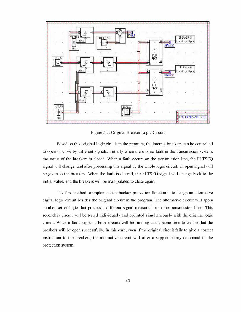
Figure 5.2: Original Breaker Logic Circuit
Based on this original logic circuit in the program, the internal breakers can be controlled
to open or close by different signals. Initially when there is no fault in the transmission system,
the status of the breakers is closed. When a fault occurs on the transmission line, the FLTSEQ
signal will change, and after processing this signal by the whole logic circuit, an open signal will
be given to the breakers. When the fault is cleared, the FLTSEQ signal will change back to the
initial value, and the breakers will be manipulated to close again.
The first method to implement the backup protection function is to design an alternative
digital logic circuit besides the original circuit in the program. The alternative circuit will apply
another set of logic that process a different signal measured from the transmission lines. This
secondary circuit will be tested individually and operated simultaneously with the original logic
circuit. When a fault happens, both circuits will be running at the same time to ensure that the
breakers will be open successfully. In this case, even if the original circuit fails to give a correct
instruction to the breakers, the alternative circuit will offer a supplementary command to the
protection system.

41
5.2.2 Microcontroller Interface
A second method of implementing the backup protection function of this project is to
apply a microcontroller interface. For accomplishing this method, a microcontroller will be using
to communicate with the main program and the breakers.
In this method, the microcontroller will consistently examine the signal port and receive
data from the main program. The main program will send a signal to the microcontroller when a
fault is detected on the transmission lines. After reading the fault detection signal from the main
program, the microcontroller will control the breakers to open immediately. In order to protect the
transmission system as soon as possible, a feasible shortest program has to be applied to the
microcontroller. Figure 5.3 below shows the logic of the completed program for this project. In
this project, an LED light will be controlled to flash by an output pin on Raspberry Pi instead of
using real breakers for demonstration.
Figure 5.3: A complete program for the microcontroller interface method

42
In section 5.3, more detailed description of the microcontroller interface method will be
provided including selection of a microcontroller, method and procedure of the implementation,
logic of the program and demonstration of the backup protection function.
An additional improvement to this method is to connect the microcontroller to the RTDS
device, and to manipulate the breakers in the relay directly by the microcontroller. By
implementing this improvement, a fully complete simulation of the project can be achieved. This
enforcement will be discussed in section 5.4.
5.2.3 Selection of Method
The method microcontroller interface has been chosen to implement the backup
protection system. Since the communication between the main program and the microcontroller is
transmitted by internet, therefore by using a microcontroller in this project, remote control can be
achieved.
The second reason is the transmission system can be more reliable by accomplishing
microcontroller interface. A microcontroller interface application is a system totally different with
the primary protection. If an alternative digital logic circuit is applied as the backup protection,
there will be a risk that both of the protection systems are failed to function. This problem is
because both of the protection systems are having exactly the same operating principle. On the
other side, when accomplishing the backup protection system by the microcontroller interface
method, a completely different system scheme will be processed. In this circumstance, the whole
protection system of the project can obtain a true double assurance.
Furthermore, a new feature of the RTDS device can be achieved with a completion of the
improvement of the microcontroller interface method.
5.3 Implementation
In this section, all the information about implementing the backup protection system is
discussed in detail. The microcontroller that is used in this project as well as the reasons of
choosing it will be introduced. Detailed description of each step of the procedure to implement
this backup protection function will also be supplied.

43
5.3.1 Microcontroller Selection
For choosing a suitable device, several popular microcontrollers in the market have been
considered and discussed from different aspects. Table 5.1 below shows a brief comparison of the
famous microcontrollers.
Table 5.1: Microcontroller Comparison
Microcontroller Raspberry Pi Arduino Uno Beagle Bone
Speed 700 MHz 16 MHz 700 MHz
RAM 256 MB 2 kB 256 MB
ROM SD card 32 Kb 4 GB Flash +
microSD card
USB 2x2.0 N/A 1x2.0
Video HDMI, NTSC, JTAG N/A N/A
Internet Interface Yes No Yes
Price $35 $39 $89
Raspberry Pi has been selected to implement the microcontroller interface part for this
project. By comparing the specification data of each microcontroller provided in the table,
apparently Raspberry Pi has huge advantages over the others.
Compare with Arduino Uno and Beagle Bone, Raspberry Pi has the highest processing
speed and the largest RAM space. Other than those advantages, Raspberry Pi is the only
microcontroller has an HDMI connection port, which will provide a much more convenient way
to monitor the operation system and interface. The two USB ports on Raspberry Pi even allow
connecting a mouse and a keyboard to control the system and create and edit any programs that
are required. On the aspect of ROM space, even though Beagle Bone has the largest ROM,
Raspberry Pi is still a strong competitor with flexible ROM selections.
The most important feature of a microcontroller for this project is the internet interface
function. In order to accomplish the completed operation, the microcontroller used in the project

44
must have the ability to connect to the internet and to receive signals from a static IP address. In
this condition, the main reason that the microcontroller Arduino Uno is not a suitable selection for
this project is because Arduino Uno does not have an internet interface function.
With regard to the prices of Beagle Bone and Raspberry Pi, Beagle Bone is almost three
times as expensive as Raspberry Pi. Nevertheless, both Beagle Bone and Raspberry Pi possess
similar and competitive of functions.
From all the comparisons above, the microcontroller Raspberry Pi is the most reasonable
and suitable device for this project.
5.3.2 Scheme and Procedure
The completed implementation of backup protection function can be divided into several
sequential parts: Raspberry Pi operating system installation, demonstration testing, Raspberry Pi
internet connection and signal receiving from the main program and the final test that combines
all the steps above as a whole. Each step of the procedure will be described in detail in this
section.
Six different operating systems are supplied on the official website of Raspberry Pi, they
are Raspbian, Pidora, RaspBMC, OpenELEC, RISC OS and Arch. The system Raspbian has been
chosen, this system is the one recommended by the Foundation and the most widely used. As a
result, there are plenty of great sources and supports around the internet for new learners. Another
reason of choosing Raspbian is this system is based on Debian, which is an extremely well
respected and capable Linux distribution, and hence Raspbian would be the easiest system to start
with.
After installing the operating system in Raspberry Pi, the second step is to test the
demonstration part. An LED light will be using for demonstration instead of real breakers. In this
step, a short program created by Python is accomplished in Raspberry Pi, where an output pin that
connected to the LED need to be assigned first, followed by a loop instructs the LED to blink.
The logic of the program for only the demonstration part is shown in Figure 5.4.

45
Figure 5.4: Program for the LED demonstration
For implementing the third step, a static IP address needs to be assigned in order to
connect Raspberry Pi to the internet. Both main program and Raspberry Pi will need to finish
setting up the IP address in the programs to obtain the communication between them. The main
program will send a signal to Raspberry Pi through the internet by the static IP address while
Raspberry Pi is running a program of continually checking the internet connection port for
receiving signals. Figure 5.5 shows the working principle of the signal receiving part. This
program is created by the language Python, the reason of using this language is because Python
code is easier to write, to read and to understand, another main reason is Python is a build-in
language in the system Raspbian.
Output pin = 1
Sleep (2)
Output pin = 0
Sleep (2)

46
Figure 5.5: Program for input signal checking in Raspberry Pi
The final step of implementing the completed backup protection system is to combine all
the previous steps with separated logic programs together and make a final test. The
demonstration program will be embedded into the signal receiving program, once a signal from
the main program is detected by Raspberry Pi, the demonstration program will automatically start
operating to light up the LED, which means to open the breakers in the transmission system. The
logic of the completed system is shown previously in figure 5.3 section 5.2.2.
5.3.3 Result
By following the scheme and the procedure described in section 5.3.2, the backup
protection function has been implemented successfully as required for the project. Although some
unexpected extra time was taken for applying and building the IP address for Raspberry Pi in the
laboratory, the whole part of implementing the backup protection system was able to be
completed on time.
5.4 Further Improvement
A further improvement of implementing the backup protection function is to connect the
microcontroller Raspberry Pi to RTDS in order to control the breakers in the relay. To accomplish
this additional function, a GTDI (Giga-Transceiver Digital Input Card) card will be needed for
Signal from
Main = true?
Yes
No
LED
demonstration
program

47
the RTDS equipment for receiving external control signals. After connecting Raspberry Pi with
RTDS by the GTDI card, Raspberry Pi will be able to communicate with RTDS directly.
When the signal of opening breakers is received by Raspberry Pi from the main program,
another new signal will be sent out from Raspberry Pi to RTDS through the GTDI card. The new
signal will be connected to the breaker function in RTDS, and when the equipment receives the
signal, the program will process the signal immediately and open the breakers in the relay. Hence
an external control of relay breakers will be built in this improvement.
For achieving a more complete simulation and RTDS device control, this improvement
will be added in the future work to this project.
5.5 Chapter Summary
The principle, method and procedure of the implementation of backup protection function
were described in detail in this chapter. The original objective and expectation of this function
have been achieved successfully for the project. The additional further improvement introduced
above in section 5.4 will also be accomplished later to obtain a more complete backup protection
implementation with RTDS.

48
Chapter 6
Windows Application
6.1 Introduction
The fault detection and location calculation algorithm described in the previous chapters
were implemented on a PC as a stand-alone windows application written in C# language. This
Fault-monitoring Program is using .NET framework and Windows Form (Winform) platform.
This Fault-monitoring Program has a size of three hundred mega-bytes with the main program,
ILNumerics numerical library and a Microsoft Access database. The development of Fault-
minitoring program has two stages: First stage program and second stage program.
The first stage Fault-monitoring Program was developed in C environment by using Cygwin
and Textpad and program which is a console application. In order to execute the code, the user
has to memorize the command. In other words, the original program is not user-friendly. The
second stage Fault-monitoring Program was implemented by using Visual studio 2012
development tools.
Compared to the first stage fault-monitoring program, the second stage program was
developed to be more feasible and advantageous. Firstly, the second stage program has an
excellent user interface, a clear distribution between the working area and library, and the
development tool is free. Secondly, the second stage program has a classic parent and child
window structure. The parent and child window structure is accessible for other developer to
insert additional functions into the library and even possible to reconstruct the working area to
adopt other purposes in the future. Thirdly, second stage Fault-monitoring Program can monitor
the status of a transmission system in real time. The program provides user high quality of plot
and animation, which allow the user to obtain a better insight during the fault condition. Fourthly,
the program can send a fault alarm message to a PC or a microcontroller in the power factory to
control the breaker in the each end of the transmission line through the internet web. This
communication channel will allowed the power system network to have a quick protection
response after the fault occur. In section 6.2, the structure of the Fault-monitoring Program is
explained in detail. The test result and the recommendations for future research are covered in
section 6.3.

49
6.2 Structure of the Program
As mentioned in the introduction, this Fault-monitoring Program is developed by using the
parent and child window structure. A child window is confined to the client area of its parent
window, an application typically uses child window to divide the client area of a parent window
into functional areas.
In the fault-monitoring program, the parent window is the main frame of the program. The
parent window is a starting window of the program; as well, this window is an archive for the
user to get access to the other functions inside the program. The user can access the parent
window by double click the icon inside the program file. Figure 6.1 is a picture for the icon.
Figure 6.2 is a picture for the fault-monitoring parent window.
Figure 6.1: Icon
Figure 6.2: Parent Window

50
Figure 6.3: Overall Structure of the Fault-monitoring Program
Figure 6.3 illustrates the Fault-monitoring Program with two parts divided inside the parent
window. The first part is the working area, which is the monitoring window. The second part is
the function library.
The monitoring window can be accessed by click the "Connection" tab in the parent window
and click "Connect the Phasor Data Concentrators". Figure 6.4 is a picture for the "Connection"
tab.
Figure 6.4: "Connection" Tab

51
Figure 6.5: Monitoring Window.
Function library can be accessed by click the "Calculator and Convertor" tab.
The data package is received by the program through the internet which is from a TCP
connection port. As Figure 6.3 shows, there are five input and output ports in the fault monitoring
program. Two of the TCP connection ports for the program are for receiving the data package
from the PDC and sending out the fault alarm message to the microcontroller in power factory.
One of the input ports for the program is for drawing the transmission line parameter from the
transmission line database. Another output port for the program is for storing the information
database of the status of the transmission system during a fault. Post fault analysis can be
provided by analyzing the voltage and current information in the database in the future. One DLL
file will hook the ILNurmerius numerical library to the program, and the ILNurmerius library will
help to accelerate the calculation process in the monitoring window.
The monitoring window or the working area is the main part of the program. The fault
detector and fault location calculator tool can be drawn from the function library in this window.
The following sections will explain the major functions in the function library.
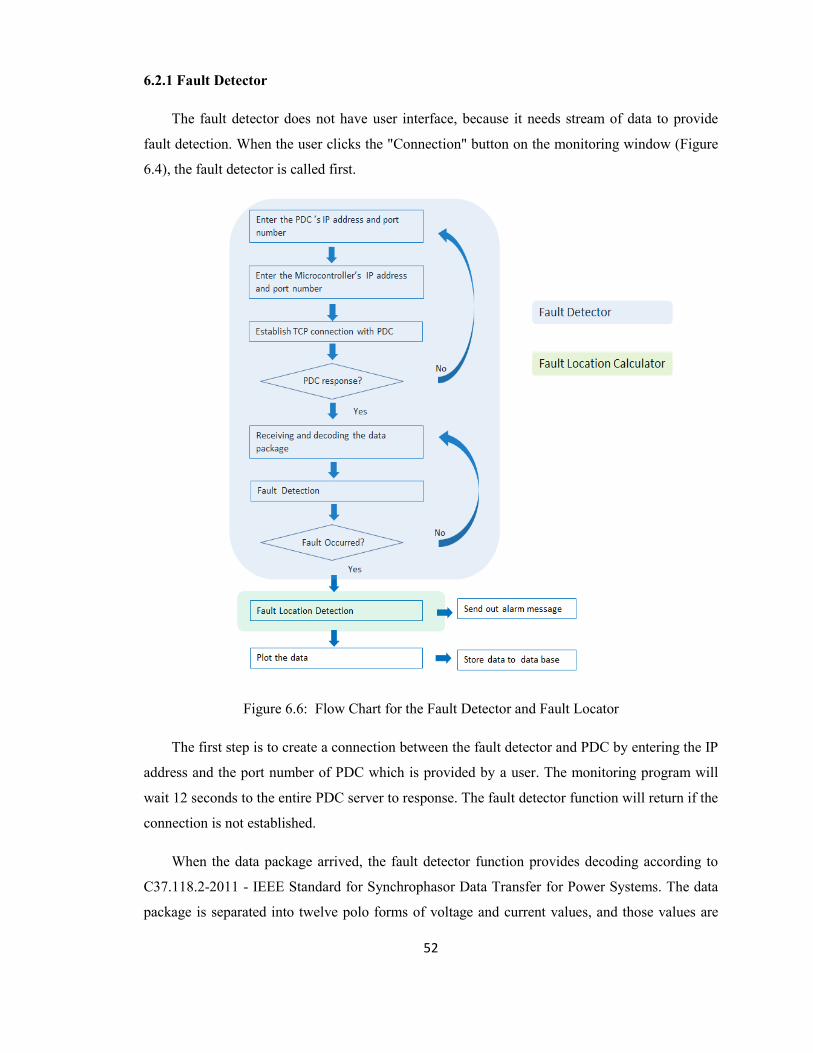
52
6.2.1 Fault Detector
The fault detector does not have user interface, because it needs stream of data to provide
fault detection. When the user clicks the "Connection" button on the monitoring window (Figure
6.4), the fault detector is called first.
Figure 6.6: Flow Chart for the Fault Detector and Fault Locator
The first step is to create a connection between the fault detector and PDC by entering the IP
address and the port number of PDC which is provided by a user. The monitoring program will
wait 12 seconds to the entire PDC server to response. The fault detector function will return if the
connection is not established.
When the data package arrived, the fault detector function provides decoding according to
C37.118.2-2011 - IEEE Standard for Synchrophasor Data Transfer for Power Systems. The data
package is separated into twelve polo forms of voltage and current values, and those values are

53
processed by using the fault detection algorithm purposed in Chapter 3 in order to detect a fault.
If a fault occurs on the transmission line is detected by the fault detector, the fault location
calculator will be called immediately to estimate the fault location on the line.
6.2.2 Fault Location Calculator
Figure 6.7: Fault Location Calculator
Users can enter a set of post fault data to calculate the fault location by using the fault
detection algorithm purposed in the chapter 4. However, during the monitoring in this program,
after the fault detector detects a fault in the power transmission line, the detector will call the fault
location calculator automatically and inject the post fault data into the fault location calculator.
The location result from the calculator is presented in a pop warning window as shown in the
Figure 6.8.

54
Figure 6.8: Warning Window
6.2.3 Fault Alarm Message
After the warning window executed, the program will return to the monitoring window. The
monitoring window acknowledges the fault in the fault detector, and the window will open the
TCP connection to the microcontroller with a static IP address and a port number. The fault alarm
message will be sent with a communication established between the monitoring window and the
microcontroller. The pre-set fault alarm message is "there is a fault" in this program and a same
message is stored in the microcontroller as well. The fault alarm message is changeable by user’s
preference in the future.
The microcontroller will compare the received message and the pre-set message to avoid
harmful programs connecting the microcontroller and falsely tripping the breaker. If the fault
alarm message is matched, the microcontroller will be aware of the fault occurred and then send a
tripping signal to the breakers.
6.2.4 Graphic User Interface, Plot and Database
The Graphic user interface is created by using Visual Studio 2012. Figure 6.9 is a screenshot
of the Visual Studio 2012 IDE.

55
Figure 6.9: Screenshot of the Visual Studio 2012 IDE
In order to create a plot of the current and voltage magnitudes verse the index number of the
data package, the program pushes all the data from the fault detector into a data collection. This
data collection is sorted by the index number of the data package, and the collection is updated
when a new data package is received. The high frequency of the update creates a real time
animation for status of a transmission line to give the user a better visual experience.
Figure 6.10: Plot of Data Package 285 During Fault Condition

56
The phase angle plot has the same principle of the current and voltage magnitude plot. The
monitoring window will convert the data inside the data collection into polo form. The
monitoring window creates a small rectangular Cartesian coordinate system in the right hand side
of the window. The monitoring window draws a line for each data such as phase A voltage. The
starting point of the line is the origin of the coordinate system, the angle of the line is the phase
angle of the data, and the length of the line is the magnitude of the data.
Figure 6.11: Phasor Diagram from the Monitor Window during the Fault Condition
Microsoft Access Database is used to store the transmission line data and the post fault data
when a fault occurs. (As shown in Figure 6.12)
Figure 6.12: Interface for the Transmission Line Database

57
6.3 Estimation Results
In this section, the performance of the fault-monitoring windows application is assessed
under different fault conditions. A simple one transmission line power system model was
simulated in RTDS. The objective is to determine a fault itself and the type and the location of the
fault using the synchrophasor measurements at the two ends of the transmission line. The currents
and voltages phasors at two ends of the transmission line are measured using the PMU in SEL-
421 relays and sent to SEL 5073 PDC.
Figure 6.13: Line to Line and Line to Ground Fault in the Simulation Model
6.3.1 Line to Line Fault
Table 6.1 Result from the Fault-monitoring Program during Phase A and B Line to Line Fault
Simulated Fault Location (Percentage of the line) 90% 80% 70% 60% 50%
Does the Fault-monitoring Program detect the fault Yes Yes Yes Yes Yes
Estimated Fault Location by the Fault-monitoring
Program
88.35% 78.17% 67.22% 59.33% 50.01%
Error 1.65% 1.83% 2.78% 0.67% 0.01%

58
Table 6.2 Result from the Fault-monitoring Program during Phase B and C Line to Line Fault
Simulated Fault Location (Percentage of the line) 90% 80% 70% 60% 50%
Is the Fault-monitoring Program detected the fault Yes Yes Yes Yes Yes
Estimated Fault Location by the Fault-monitoring
Program
87.22% 77.09% 68.03% 59.06% 50.08%
Error 2.78% 2.91% 1.77% 0.94% 0.08%
Table 6.3 Result from the Fault-monitoring Program during Phase A and C Line to Line Fault
Simulated Fault Location (Percentage of the line) 90% 80% 70% 60% 50%
Is the Fault-monitoring Program detected the fault Yes Yes Yes Yes Yes
Estimated Fault Location by the Fault-monitoring
Program
88.90% 79.15% 67.19% 59.34% 49.78%
Error 1.10% 0.85% 2.81% 0.66% 0.22%
Table 6.4 Result from the Fault-monitoring Program during Phase A, B and C Line to Line Fault
Simulated Fault Location (Percentage of the line) 90% 80% 70% 60% 50%
Is the Fault-monitoring Program detected the fault Yes Yes Yes Yes Yes
Estimated Fault Location by the Fault-monitoring
Program
88.23% 79.46% 68.77% 59.42% 49.17%
Error 1.77% 0.54% 1.23% 0.58% 0.83%

59
6.3.2 Line to Ground Fault
Table 6.5: Result from the Fault-monitoring Program during Phase A Line to Ground Fault
Simulated Fault Location (Percentage of the line) 90% 80% 70% 60% 50%
Is the Fault-monitoring Program detected the fault Yes Yes Yes Yes Yes
Estimated Fault Location by the Fault-monitoring
Program
87.44% 77.69% 67.98% 58.53% 50.10%
Error 2.56% 2.31% 2.02% 1.47% 0.10%
Table 6.6: Result from the Fault-monitoring Program during Phase B Line to Ground Fault
Simulated Fault Location (Percentage of the line) 90% 80% 70% 60% 50%
Is the Fault-monitoring Program detected the fault Yes Yes Yes Yes Yes
Estimated Fault Location by the Fault-monitoring
Program
88.33% 77.15% 69.03% 59.80% 50.03%
Error 1.67% 2.85% 0.97% 0.02% 0.03%
Table 6.7: Result from the Fault-monitoring Program during Phase C Line to Ground Fault
Simulated Fault Location (Percentage of the line) 90% 80% 70% 60% 50%
Is the Fault-monitoring Program detected the fault Yes Yes Yes Yes Yes
Estimated Fault Location by the Fault-monitoring
Program
87.17% 77.07% 68.92% 58.66% 49.68%
Error 2.83% 2.93% 1.08% 1.34% 0.32%

60
Table 6.8: Result from the Fault-monitoring Program during Phase A and B Line to Ground Fault
Simulated Fault Location (Percentage of the line) 90% 80% 70% 60% 50%
Is the Fault-monitoring Program detected the fault Yes Yes Yes Yes Yes
Estimated Fault Location by the Fault-monitoring
Program
88.08% 79.23% 68.81% 59.13% 49.84%
Error 1.92% 0.77% 1.19% 0.87% 0.16%
Table 6.9: Result from the Fault-monitoring Program during Phase A and B Line to Ground Fault
Simulated Fault Location (Percentage of the line) 90% 80% 70% 60% 50%
Is the Fault-monitoring Program detected the fault Yes Yes Yes Yes Yes
Estimated Fault Location by the Fault-monitoring
Program
87.84% 78.33% 68.16% 59.39% 50.25%
Error 2.16% 1.67% 1.84% 0.61% 0.25%
Table 6.10: Result from the Fault-monitoring Program during Phase A and C Line to Ground
Fault
Simulated Fault Location (Percentage of the line) 90% 80% 70% 60% 50%
Is the Fault-monitoring Program detected the fault Yes Yes Yes Yes Yes
Estimated Fault Location by the Fault-monitoring
Program
88.10% 77.56% 69.21% 59.23% 50.52%
Error 1.90% 2.44% 0.79% 0.77% 0.52%

61
6.3.3 Three Phases to Ground Fault
Table 6.11: Result from the Fault-monitoring Program during three Phases to Ground Fault
Simulated Fault Location (Percentage of the line) 90% 80% 70% 60% 50%
Is the Fault-monitoring Program detected the fault Yes Yes Yes Yes Yes
Estimated Fault Location by the Fault-monitoring
Program
88.83% 78.77% 68.74% 58.25% 49.55%
Error 1.17% 1.23% 1.26% 1.75% 0.45%
The results of the fault detection and fault location by operating the Fault-monitoring
Program are extremely promising as shown in the tables above. The maximum error in the fault
location estimation is 2.91% which is lower than the specification of this project, and the
accuracy of the fault detection is 100%. Compared the results from Fault-monitoring Window
with SEL-421 (Hardware PMU) to the results producing from PMU Model in RSCAD (section
4.7), the result from Hardware PMU has higher measured error percentage than error found in
Chapter 4. This situation is expected, because the Hardware PMU has more sources of errors,
such as time difference due to GPS clock, hardware imperfections; however, the result from PMU
model is more closed the ideal case without considering the practical environment.
6.4 Future Works
The best plot for the user visualization is the current and voltage verse the time stamp inside
the data package. Such plot is extremely hard to archive due the complex format of the time
stamp, for example, the format of ten o’clock is “10:00:00.00", but the colon symbol in the C#
language has a different meaning. The best solution is converting the time format into a String.
However, in that way the program will treat the time stamp as a sentence. A string format of time
will loss the original purpose to serve as a time stamp, ten o'clock will be no different as other
time stamp, such as ten fifteen or nine o'clock, because they are all sentences in the program's
point of view. Thus, the program cannot create a plot with sentences instead of values, and the
program will have an extremely high difficulty of tracking itself.
An advantageous and meaningful plot need to be developed in the future, it can be done by
using a different approach such as split the time stamp into four parts: hours, minutes and second

62
and fraction of seconds. The program will calculate the time stamp for each part and combine
every part in the end of plotting.
6.5 Chapter Summary
In this chapter, a fault-monitoring windows application using synchrophasor measurements
was presented. The structure of this application includes a fault detector, a fault location
calculator, a graphic user interface, a database and a fault alarm message. Each part was
introduced in details in this chapter. A number of tests were performed to validate the fault-
monitoring windows application. The test results confirmed the accuracy of the algorithm and
implementation.
63
Chapter 7
Conclusion
The project has been accomplished the differential protection algorithm using
synchronized current measurements and implement it on real time hardware. The total cost of
project is within budget (detail see Appendix E). Overall, the following tasks of project have been
achieved.
Firstly, a power system network model with analog outputs interface with PMUs has
been successfully designed. The interface program is able to extract the required phasor data from
PDC.
Secondly, based on the time assessment and accuracy evaluation, Current Scalar
Summation Method with shortest time-consuming and highest performance is utilized as
differential protection algorithm for major-transmission line in this study.
Thirdly, Phasor Based Method is evaluated to identify the location of fault and it is
proven to be no affected by various system situations such as fault types, fault impedances and
fault locations as well as achieve the high degree of accuracy. The fault location result of
algorithm and hardware testing reaches the Specification (Table 1.1) which is within 5% error.
Fourthly, the principle, method and procedure of the implementation of backup
protection function were studied, the microcontroller Raspberry Pi achievable sends trip signal to
the breaker through IP network and indicates the fault message as flashing LED light. In future, a
further improvement of implementing the backup protection function is to connect the
microcontroller Raspberry Pi to RTDS in order to control the breakers in the relay.
Fifthly, A user-friendly window application was developed by group, this window
application was embedded all the project scope functions discussed above, which includes the
fault detection, fault type identification, fault alarm, fault location measurement and backup
protection. The window application is stable which had be verified above 99% stability, also, it
has not been crash once during more five hundred tests, therefore reliability of this application
reaches the Specification (Table 1.1). An advantageous plot in the window application needs to
be developed in the future; the plot will be upgraded to include the time stamp inside the data
package.

64
Bibliography
[1] A. Guzman, S. Samineni, M. Bryson, “Protective Relay Synchrophasor Measurements During
Fault Conditions,” in Power Systems Conference: Advanced Metering, Protection, Control,
Communication, and Distributed Resources, 2006. PS’06, 2006, pp. 83–95.
[2] M. M. Saha, J. Izykowski, E. Rosolowski, "Two-end Fault Location on Series compensated
Lines”, Fault Location on Power Networks, New York, Springer-Verlag London, 2010, ch. 7, pp.
263-329.
[3] RTDS Simulator Applications, RTDS Technologies Inc. Available:
http://www.rtds.com/applications/applications.html.
[4] RTDS Hardware Manual, Rev 0, RTDS Technologies, Winnipeg, MB, 2009, pp. 7.1-7.30.
[5] J.M. Gers, E.J. Holmes, “Current and Voltage Transformers,” in Protection of Electricity
Distribution Networks, 2nd ed. London, United Kingdom: The Institution of Electrical
Engineering and Technology, 2004, ch. 4, sec. 4.1, pp. 47-51.
[6] M. Nezammahaleh, H. Javadi, M. Khederzadeh, “Differential Protection of Transmission
Lines Compensated by Series (SSSC), Shunt (STATCOM) and Series-Shunt Branches of UPFC.
Part I: Uncompensated Transmission Line,” International Review on Modelling and Simulations
(I.RE.MO.S.), Vol. 5, N. 1, Feb. 2012, pp. 270-277.
[7] V.S. Kale, S.R. Bhide, P.P. Bedekar, “Faulted Phase Selection on Double Circuit
Transmission Line using Wavelet Transform and Neural Network” , Third International Conf. on
Power Syst., Kharagpur, ICPS, Dec 2009, pp. 1-6.
[8] M.M. Saha, J. Izykowski, E. Rosolowski, “Phase Selection,” Fault Location on Power
Networks, New York, Springer-Verlag London, 2010, pp. 90-95.
[9] W. Haigang, X. Z. Dong, Z. Q. Bo, B. R. J. Caunce, and A. Klimek,“An operation criterion
for line current differential relay with higher sensitivity,” in Proc. IEEE Power Eng. Soc. General
Meet., Montreal, QC, Canada, 2006, pp. 1–6.
[10] A.T.Johns, S.Jamali, "Accurate fault location technique for power transmission lines",
Generation, Transmission and Distribution, IEEE Proceedings C, vol.137, no.6, pp. 395 - 402,
November. 1990.

65
[11] R.K. Aggarwal, D.V. Coury, A.T. Johns, A. Kalam, "A practical approach to accurate fault
location on extra high voltage teed feeders", Power Delivery, vol.8, no.3, pp. 95-108, July. 1993.
[12] K. Zimmerman, D. Costello, "Impedance-based fault location experience", 58th Annual
Conference for Protective Relay Engineers, Vol. 5, N. 1, April 2005, April 2005, pp.211-226.
[13] J.Berdy, Local Back-up Protection for an Electric Power System. [Online] Ontario, Canada. Available: http://store.gedigitalenergy.com/faq/Documents/D60/GER-3178.pdf [Feb 25, 2014]
[14] Schweitzer Engineer Laboratories, Inc. (2013, Dec 31). SEL-421-4, -5 Data Sheet. [Online]. Available: https://www.selinc.com/SEL-421/ [Feb 25, 2014]
[15] IEEE Standard for Synchrophasor Data Transfer for Power Systems, IEEE Std C37.118.2-
2011 (Revision of IEEE Std C37.118-2005), pp. 153, 2011.
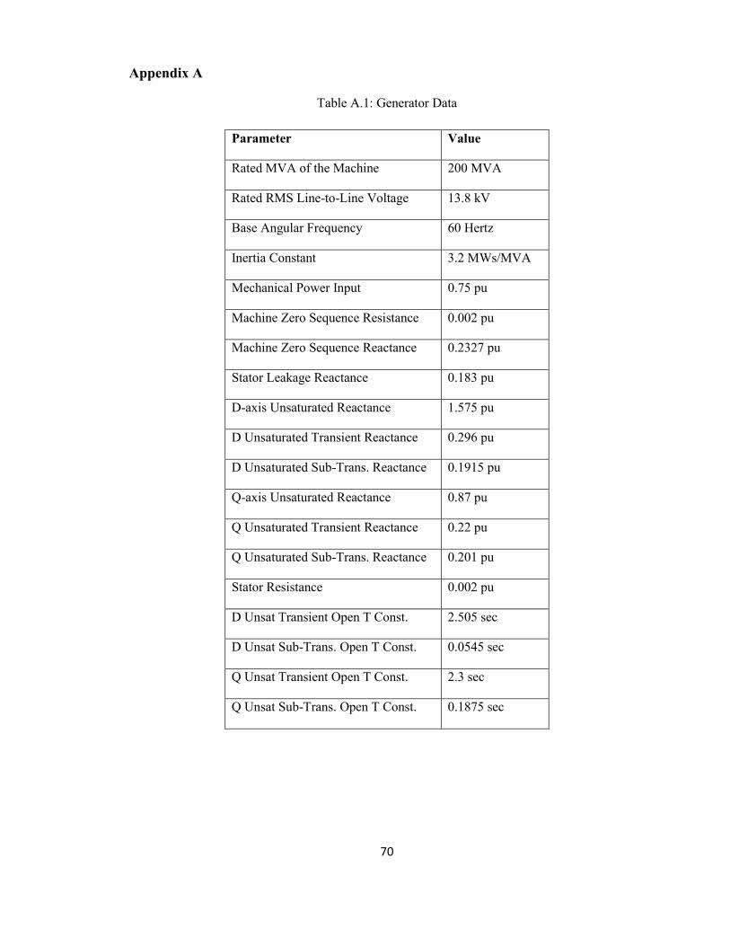
70
Appendix A
Table A.1: Generator Data
Parameter Value
Rated MVA of the Machine 200 MVA
Rated RMS Line-to-Line Voltage 13.8 kV
Base Angular Frequency 60 Hertz
Inertia Constant 3.2 MWs/MVA
Mechanical Power Input 0.75 pu
Machine Zero Sequence Resistance 0.002 pu
Machine Zero Sequence Reactance 0.2327 pu
Stator Leakage Reactance 0.183 pu
D-axis Unsaturated Reactance 1.575 pu
D Unsaturated Transient Reactance 0.296 pu
D Unsaturated Sub-Trans. Reactance 0.1915 pu
Q-axis Unsaturated Reactance 0.87 pu
Q Unsaturated Transient Reactance 0.22 pu
Q Unsaturated Sub-Trans. Reactance 0.201 pu
Stator Resistance 0.002 pu
D Unsat Transient Open T Const. 2.505 sec
D Unsat Sub-Trans. Open T Const. 0.0545 sec
Q Unsat Transient Open T Const. 2.3 sec
Q Unsat Sub-Trans. Open T Const. 0.1875 sec

71
Table A.2: Transformer Data
Parameter Value
Winding 1 Connection Delta
Winding 2 Connection Wye
Delta lags or leads Y Lags
Transformer rating (3 Phase) 210 MVA
Base Frequency 60 Hz
Leakage Inductance of Tx 0.152 pu
Nominal primary voltage (L-L RMS) 220 kV
Nominal secondary voltage (L-L RMS) 13.8 kV
Table A.3: Transmission Line data
Parameter Value
Number of Phases 3
Positive Sequence Series Resistance 0.09756 Ohm/km
Positive Sequence Series Ind. Reactance 0.41346 Ohm/km
Positive Sequence Shunt Cap. Reactance 0.3636800653 Megaohms*km
Zero Sequence Series Resistance 0.27565 Ohm/km
Zero Sequence Series Ind. Reactance 1.33356 Ohm/km
Zero Sequence Shunt Cap. Reactance 0.567093032409 Megaohms*km
Line length 207 km

72
Appendix B
Table B.1: Current Transformer Data
Parameter Value
Secondary Side Resistance 0.5 Ohms
Secondary Side Inductance 8.00E-04 H
Turns Ratio 240
Burden series resistance 1.62 Ohms
Burden series inductance 2.08E-03 H
Table B.2: Potential Transformer Data
Parameter Value
Primary Side Resistance 11.33 Ohm
Primary Side Inductance 6 H
Primary Side Turns 230000 turns
Secondary Side Resistance 5.50E-04 Ohm
Secondary Side Inductance 2.90E-04 H
Secondary Side Turns 115 turns
Burden series Resistance 4.55 Ohm
Burden series Inductance 5.30E-04 H
Burden parallel Resistance 2298 Ohm

73
Table B.3: Capacitive Voltage Transformer Data
Parameter Value
Primary Side Resistance 474 Ohm
Primary Side Inductance 4.46 H
Primary Side Turns 11000 turns
Secondary Side Resistance 0.18 Ohm
Secondary Side Inductance 4.70E-04 H
Secondary Side Turns 115 turns
Burden series resistance 400.9 Ohm
Burden series inductance 1.84 H
Burden parallel resistance 2298 Ohm
Table B.4: Ferro-resonance Filter Data
Parameter Value
Rf1 1.06 Ohm
Lf1 0.01 H
Cf 8 μF
Rf2 4.24 Ohm
Lf2 0.394 H
Rf 40 Ohm

74
Appendix C
Table C.1: Global Settings for the SEL-421
General Global Settings PMU 1 PMU 2
Station Identifier Station A Station B
Relay Identifier SEL 421 SN
2009063232
SEL-421 SN
2009063233
Nominal System Frequency 60 60
System Phase Rotation ABC ABC
Settings Group Selection PMU 1 PMU 2
SS1 Select Setting Group 1 SG1 SG1
Frequency Estimation PMU1 PMU2
Local Frequency Source 1 VAY VAY
Local Frequency Source 2 VBY VBY
Local Frequency Source 3 VCY VCY
Current and Voltage Source Selection PMU1 PMU2
Line Current Source IW IW
Synchronized Phasor Measurement PMU1 PMU2
Enable Synchronized Phasor Measurement Yes Yes
Message Format C37.118 C37.118
Message per Second 30 30
PMU Application Narrow Bandwidth Narrow Bandwidth
Station Name STATION A STATION B
PMU Hardware ID 1 2
Phasor Data Set, Voltages ALL ALL
Phasor Data Set, Currents ALL ALL
Current source BOTH BOTH
Phasor Numeric Representation Integer Integer
Phasor Format Rectangular Rectangular
Frequency Numeric Representation Integer Integer
Messages per Second 30 30
Time and Date Management C37.118 C37.118

75
Table C.2: Transmission Line Parameter Settings for the SEL-421
Positive Sequence Impedance Ω/km Ω Degrees
Series Resistance 0.09756 20.19492 N/A
Series Inductive Reactance 0.41346 85.58622 N/A
Magnitude N/A 87.93 N/A
Angle N/A N/A 76.72
Zero Sequence Impedance Ω/km Ω Degrees
Series Resistance 0.27565 57.05955 N/A
Series Inductive Reactance 1.33356 276.04692 N/A
Magnitude N/A 281.88 N/A
Angle N/A N/A 78.32
Line Length 207 km
Table C.3: Transmission Line Parameter Settings in Secondary Ohms for the SEL-421
Setting Magnitude (Secondary Ω) Degrees
Positive Sequence Impedance 10.55 76.72
Zero Sequence Impedance 33.83 78.32
Table C.4: Line Configuration Parameter Settings for the SEL-421
Line Configuration PMU1 PMU2
Current Transformer Ratio 240 240
Potential Transformer Ratio 2000 2000
PT Nominal Voltage L-L (V, s) 115 115
Positive Sequence Line Impedance Magnitude (Ω, s) 10.55 10.55
Positive Sequence Line Impedance Angle (Degrees) 76.72 76.72
Zero Sequence Line Impedance Magnitude (Ω, s) 33.83 33.83
Zero Sequence Line Impedance Angle (Degrees) 78.32 78.32
Line Length (km) 207 207

76
Appendix D
Table D.1: Communication Settings for the SEL-421
Settings PMU1 PMU2
IP Address 130.179.228.99 130.179.228.100
Subnet mask 255.255.252.000 255.255.252.000
Default router 130.179.228.001 130.179.228.001
Enable Synchrophasors Over Ethernet Yes Yes
PMU Output 1 Transport Scheme TCP TCP
PMU Output 1 Client (Remote) IP Address
130.179.231.223 130.179.231.223
PMU Output 1 TCP/IP (Local) Port 4722 4722
Table D.2: Serial Port F Communication Settings
Parameter Value
Data Speed (bps) 9600
Data Bits 8
Parity None
Stop Bits 1
Enable Hardware Handshaking No

77
Appendix E
Table E: Budget
Component Unit Cost Quantity Supplied By Actual Cost
RTDS unit $1,000,0001 1 NSERC CRSNG2 $0
SEL-421 Relay $6250.00 2 NSERC CRSNG2 $0
Microcontroller $39 1 Yaojie $0
Computer Screen $286 1 Advisor $0
Keyboard $15 1 Advisor $0
Mouse $15 1 Advisor $0
SD card $30 1 U of M $30
Total (plus tax) $1,144,560.05 $33.90
1 The cost of the RTDS unit shown in the table is a rough estimate only. 2 NSERC CRSNG-Natural Sciences and Engineering Research Council of Canada
The sponsor of major research equipment to University of Manitoba is NSERC
CRSNG. We had been authorized to use equipment such as the RTDS unit and the SEL-
421 relays.