synchrotron radiation for beam diagnostics: numerical ... · synchrotron radiation for beam...

Synchrotron radiation for beam diagnostics: Numerical

calculations of the single electron spectrum

Oliver GrimmUniversity of Hamburg

June 18, 2008

Abstract

This paper presents a simple numerical algorithm to calculate single-electron synchrotronradiation spectra resulting from acceleration in an arbitrary magnetic field. The focus is on anexact implementation of the basic formula governing the emission, not on fast computation.Comparisons to several analytical calculations are made, and some results applicable for theFLASH free-electron laser are given.

1 Introduction

Synchrotron radiation has many applications in electron beam diagnostics. It allows measure-ments of the transverse and longitudinal structure of electron bunches, as well as the energydistribution. The radiation is emitted fully parasitically in dipole magnets that are present incircular as well as linear accelerators or storage rings. The wide spectral range that makes itdesirable as a source in its own right also is attractive for beam diagnostics.

Especially for longitudinal electron beam diagnostics using coherent radiation techniques, acomprehensive understanding of the single-electron spectrum is required, as this is needed tounfold the measured spectra and to deduce or asses the longitudinal charge distribution [Gri06].1

This report summarizes the basics of synchrotron radiation calculations, presents a simple codeto numerically derive the single-electron spectrum, and gives several results applicable to thefree-electron laser FLASH at DESY.

The typical synchrotron radiation pulse duration is of the order of picoseconds or less, atime-scale that usual (bolometric) radiation detectors cannot resolve. It is therefore not theinstantaneous power that is relevant, but the energy within a pulse. Frequency is always givenas cycle frequency, not angular frequency. The Fourier transform of a function is designated withthe same symbol as the function itself, only distinguished by its variable. All calculations aredone in SI units.

Sect. 2 presents the necessary background for the calculation of synchrotron radiation spectraand lists some analytical calculations. Sect. 3 then details the numerical algorithm and some basicresults. Several calculations relevant explicitly for FLASH are summarized in Sect. 4. Additionaltheoretical material is collected in the appendices.

1Note that the derivation in this report explicitly requires that each electron radiates the same electric field intime domain, only shifted according to its longitudinal position within the bunch. This is not always guaranteedif the magnetic field changes rapidly and the head of the bunch can be subject to varying fields from the tail[Sal97]. More elaborate numerical simulations than reported here are necessary under such circumstances, takinginto account the self-interaction within the bunch.

1

TESLA-FEL Report 2008-05

Most explicit calculations presented will use the nominal parameters of a dipole of the firstFLASH bunch compressor chicane: magnetic field 0.27 T, giving a bending radius of 1.6 m at130 MeV. The effective length of such a dipole is 50 cm, resulting in a nominal deflection of 18°.

2 Single-electron spectrum: Basics and analytical calculations

2.1 General magnetic field

Synchrotron radiation is emitted by a relativistic electron accelerated transversely to its motionby passing a magnetic field. The starting point for the calculation of the emission spectrumresulting from an arbitrary magnetic field are the retarded Lienard-Wiechert potentials [Jack75].They give the electric and magnetic field resulting from a general acceleration of an elementarycharge at some observation point as2

�E(t) =e

4πε0

�n(t) − �β(t)

γ2(1 − �β(t)·�n(t))3L2(t)

∣∣∣∣∣ret

+e

4πε0c

�n(t) × ((�n(t) − �β(t)) × �β(t))

(1 − �β(t)·�n(t))3L(t)

∣∣∣∣∣ret

(1a)

�B(t) =1c

�n(t)|ret × �E(t), (1b)

where the velocity �β = �v/c, the acceleration �β, the unit vector �n from the charge to the obser-vation point, and the corresponding distance L all need to be evaluated at the retarded timet′ = t − L(t′)/c to account for the finite propagation velocity. The first part of �E(t) is usuallycalled the velocity term, the second the acceleration term.

The power flow in time-domain follows from the Poynting vector �S(t), given in free space by(see App.A.1)

�S(t) =1μ0

�E(t) × �B(t) = ε0c(| �E(t)|2 �n(t)|ret − (�E(t) · �n(t)|ret)�E(t)

). (2)

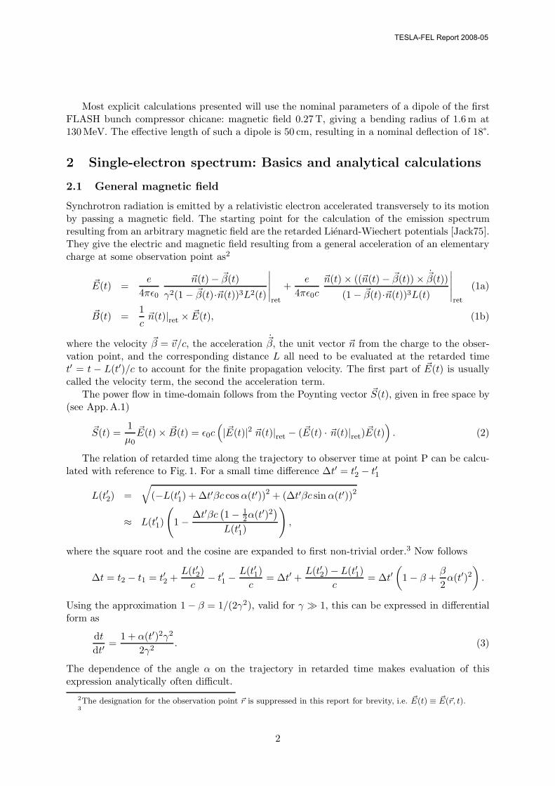
The relation of retarded time along the trajectory to observer time at point P can be calcu-lated with reference to Fig. 1. For a small time difference Δt′ = t′2 − t′1

L(t′2) =√

(−L(t′1) + Δt′βc cos α(t′))2 + (Δt′βc sin α(t′))2

≈ L(t′1)

(1 − Δt′βc

(1 − 1

2α(t′)2)

L(t′1)

),

where the square root and the cosine are expanded to first non-trivial order.3 Now follows

Δt = t2 − t1 = t′2 +L(t′2)

c− t′1 −

L(t′1)c

= Δt′ +L(t′2) − L(t′1)

c= Δt′

(1 − β +

β

2α(t′)2

).

Using the approximation 1 − β = 1/(2γ2), valid for γ � 1, this can be expressed in differentialform as

dt

dt′=

1 + α(t′)2γ2

2γ2. (3)

The dependence of the angle α on the trajectory in retarded time makes evaluation of thisexpression analytically often difficult.

2The designation for the observation point �r is suppressed in this report for brevity, i.e. �E(t) ≡ �E(�r, t).3

2


Pα(t′)

t′1

t′2

L(t′1)

L(t′2)

Figure 1 General trajectory to illustrate the relation between retarded and observer time.

At large distance from a source region, the second term on the right side of (2) is absentsince then �E(t) is perpendicular to �n(t′) due to the faster reduction of the first term in (1a) withdistance than the second.

The frequency spectrum follows through application of a Fourier transformation,

�E(ν) =

∞∫−∞

�E(t)e−2πiνt dt, (4)

giving the energy density spectrum in units of J/(Hzm2) at a given position at large distanceas (see App.A)

d2U

dνdA≈ 2ε0c| �E(ν)|2. (5)

It should be noted that the labeling of the acceleration term as ’radiation term’, as is some-times done, is not entirely correct, since some part of the radiated field energy contained in thevelocity term at small distances ends up in the acceleration term at larger distance once theformer has died out due to its stronger dependence on distance. A charge in uniform motionwill carry of course only the velocity field along and does not lose energy. An accelerated chargewill have a different behaviour of the velocity vector �β and of the unit vector �n in the first termof (1a). The electric field contribution of this term is modified compared to the non-radiatingcase, thus contributing partly to the energy lost by the particle. Although at large distance allradiated power is accounted for by the acceleration term of (1a), part of that power appears inthe velocity term at smaller distance. The velocity term does not only contain the static field.

2.2 Asymptotic expressions

The emitted radiation spectrum depends on the acceleration of the electron, which in turn isan effect of the magnetic field (see App.C). Clearly, no general solution for arbitrary magneticfields can be given. However, several asymptotic expressions have been derived by various au-thors. These are useful not only for understanding the basic principles of synchrotron radiationgeneration, but also as benchmarks to test the performance and correct operation of numericalcodes. Some of these asymptotic results will be briefly summarized in this section.

2.2.1 Synchrotron radiation from circular motion

Using the approximations

• Constant magnetic field: The particle follows a circular trajectory (radius R).

3


• Large distance of the observation point from the source region: �n and L are constant intime and only the acceleration term in (1a) is considered.

• Highly relativistic motion (γ � 1): The radiation is emitted in a narrow cone.

the angular spectral energy distribution of a single electron is calculated in [Jack75]:(d2U

dλdΩ

)c.m.

=2e2

3ε0

R2

λ4

(1γ2

+ Θ2

)2(K2

2/3(ξ) +Θ2

1/γ2 + Θ2K2

1/3(ξ))

, (6)

where ξ =2πR

3λ

(1γ2

+ Θ2

)3/2

.

The first term in brackets refers to horizontal polarization (in the orbit plane), the second termto vertical polarization and Θ is the vertical observation angle. There is clearly no dependenceon the horizontal angle for circular motion. Angle-integrating this yields

(dU

dλ

)c.m.

=√

3e2

2ε0

γλc

λ3

∞∫λc/λ

K5/3(x)dx, where λc =4πR

3γ3. (7)

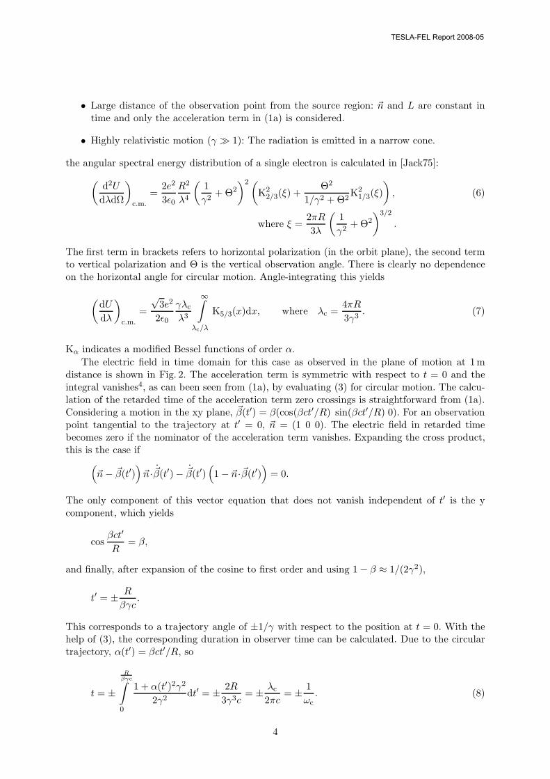
Kα indicates a modified Bessel functions of order α.The electric field in time domain for this case as observed in the plane of motion at 1m

distance is shown in Fig. 2. The acceleration term is symmetric with respect to t = 0 and theintegral vanishes4, as can been seen from (1a), by evaluating (3) for circular motion. The calcu-lation of the retarded time of the acceleration term zero crossings is straightforward from (1a).Considering a motion in the xy plane, �β(t′) = β(cos(βct′/R) sin(βct′/R) 0). For an observationpoint tangential to the trajectory at t′ = 0, �n = (1 0 0). The electric field in retarded timebecomes zero if the nominator of the acceleration term vanishes. Expanding the cross product,this is the case if(

�n − �β(t′))

�n· �β(t′) − �β(t′)(1 − �n·�β(t′)

)= 0.

The only component of this vector equation that does not vanish independent of t′ is the ycomponent, which yields

cosβct′

R= β,

and finally, after expansion of the cosine to first order and using 1 − β ≈ 1/(2γ2),

t′ = ± R

βγc.

This corresponds to a trajectory angle of ±1/γ with respect to the position at t = 0. With thehelp of (3), the corresponding duration in observer time can be calculated. Due to the circulartrajectory, α(t′) = βct′/R, so

t = ±R

βγc∫0

1 + α(t′)2γ2

2γ2dt′ = ± 2R

3γ3c= ± λc

2πc= ± 1

ωc. (8)

4


−8 −6 −4 −2 0 2 4 6 8

x 10−16

−16

−14

−12

−10

−8

−6

−4

−2

0

2

4

6

Observer Time (s)

Ele

ctric

fiel

d (V

/m)

Acceleration termVelocity term (x100)

Figure 2 Electric field for the case of circular motion. The observation point is on the bendingplane at 1m distance tangentially, electron energy 130 MeV, bending radius 1.6 m. The weakfield from the velocity term, shown multiplied by 100, is disregarded in the usual calculation ofthe radiation spectrum.

The electric field zero crossings occur thus at a time equal to the inverse of the critical angular fre-quency ωc. For the parameters of a FLASH bunch compressor dipole, this yields t=±2.2×10−16 s,as seen in Fig. 2.

The peak electric field in forward direction can also easily be deduced from (1a), using (18)and the fact that �n is parallel to the velocity and perpendicular to the acceleration at t = 0:

E(0) =−e2

πε0mc

γ3B

L=

−eγ4

πε0LR.

The emitted power during the motion along the circle is

P =e2c

6πε0

γ4

R2. (9)

This expression remains valid as the instantaneous power in case the magnetic field and thusthe radius changes. Integration over the trajectory will give the total energy lost by the particle.

For long wavelengths λ � λc, often of particular interest for coherent radiation diagnostics,(6) becomes for Θ = 0(

d2U

dλdΩ

)l.w.

=e2

2ε0

(Γ(2/3)

π

)2(34

)1/3 (2πR)2/3

λ8/3,

which is independent of energy for a given radius of curvature. The typical opening angle in thiscase is

Θl.w. =1γ

(λ

λc

)1/3

=(

3λ2πR

)1/3

, (10)

4This is why the spectrum drops to zero at zero frequency, as �E(ν = 0) =�∞−∞

�E(t) dt.

5


which is also independent of energy.These formulae give the spectrum resulting from a single passage of the electron. Strictly, the

integration in (4) runs from -∞ to ∞, and for circular motion a line spectrum results, consistingof harmonics of the revolution frequency. This can be seen by writing for 2m revolutions ofperiod t0, where m is a positive integer,

�E2m(ν) =

mt0∫−mt0

�E(t)e−2πiνt dt =m∑

k=−m

(k+1)t0∫kt0

�E(t)e−2πiνt dt

=m∑

k=−m

t0∫0

�E(t + kt0)e−2πiν(t+kt0) dt =m∑

k=−m

e−2πiνkt0

t0∫0

�E(t)e−2πiνt dt

=

(2

m∑k=1

cos(2πνkt0) + 1

) t0∫0

�E(t)e−2πiνt dt,

The relation �E(t + kt0) = �E(t) for any integer k is used. The emitted energy will be infinite foran infinite number of revolutions, therefore the power frequency spectrum is a more appropriatequantity:

I2m(ν) =2ε0c| �E2m(ν)|2(2m + 1)t0

= (2m + 1)I0(ν)

⎛⎜⎜⎝

2m∑

k=1

cos(2πνkt0) + 1

2m + 1

⎞⎟⎟⎠

2

.

I0(ν) is the averaged power spectrum from a single passage. The term in brackets representsa line spectrum at integer multiplies of 1/t0, with unit amplitude, and a line width decreasingwith increasing m. The envelope of the spectrum remains the same as for a single passage, butthe power is concentrated into progressively narrower frequency spikes.

2.2.2 Low-frequency radiation

In [Meot99], the low-frequency limit of the synchrotron radiation spectrum for a constant mag-netic field of finite extend is calculated by neglecting the exponential term in (4) altogether andusing only the acceleration term in (1a):

�E(ν) =∫Δt

�E(t) dt.

Clearly, this is frequency independent. The validity requirement νΔt � 1, where Δt is theduration of the radiation pulse, can be expressed using the length of the magnetic field regionL and the (typical) curvature radius ρ as

ν � γ2c

πL(1 + γ2L2

12ρ2

) .

For the parameters of a bunch compressor dipole, this yields ν � 150GHz, so that the validityis confined to wavelengths were the chamber cut-off (to be discussed below) already completelysuppresses the spectrum. Except for benchmarking, this approximation is of no further use forapplication at FLASH.

6


2.2.3 Short magnet radiation

The far-field radiation spectrum for a weak magnet has been calculated analytically in [Coı79].The main steps of the derivation are outlined here.

The acceleration of an electron by a magnetic field of constant direction, �Bm(t) = Bm(t)�nm,is, from (18),

�β(t) =eBm(t)

mγ�β(t)×�nm.

The subscript m is used to clearly distinguish this static field from the emitted magnetic field(1b). The time-dependence of �Bm(t) results from the movement of the electron through thespatially varying field. Neglecting now all time dependences in (1a) except that of the magneticfield magnitude which enters via the acceleration, and considering only the acceleration term,the electric field in time-domain can be written as

�E(t) =e2

4πε0mc

�n ×{(

�n − �β)×(�β×�nm

)}γ(1 − �β ·�n)3L

Bm(t)|ret .

The disregard of the time dependence of �n and L along with the velocity term implies a largedistance of the observation point to the magnetic field region. The disregard of the time depen-dence of �β additionally requires that the angle of the trajectory is changed much less than 1/γ,which is the case for a short or weak magnet. With this condition (3) can be evaluated easily, asthen α is constant, and so the compression between retarded and observer time is also constant:dt/dt′ = t/t′. Now

∞∫−∞

Bm(t)|ret e−2πiνt dt =1 + α2γ2

2γ2

∞∫−∞

Bm(t′)e−2πiν 1+α2γ2

2γ2 t′ dt′,

and the Fourier transform of �E(t) can thus be written as

�E(ν) =e2

πε0mcL

γ3

(1 + α2γ2)2�n ×

{(�n − �β

)×(

�β×�nm

)} ∞∫−∞

Bm(t′)e−2πiν 1+α2γ2

2γ2 t′ dt′.

This requires only an integration along the particle trajectory. The double cross product can besimplified according to

�n ×{(

�n − �β)×(�β×�nm

)}= �n ×

{�β (�n · �nm) − �nm

(�n · �β

)− �β

(�β · �nm

)+ �nmβ2

}= �n ×

{�β (�n · �nm) − �nm

(cos α − β2

)}= �n × �β (�n · �nm) − �n × �nm

(1γ2

− α2

2

).

The assumption has been made that the velocity is perpendicular to the magnetic field.The requirement of a small change in trajectory direction is often not desirable for beam

diagnostics purposes, as it will complicate outcoupling of the radiation that will almost co-propagate with the electron beam. A mirror with a small hole can be used that however needsto be inside of the ultra-high machine vacuum. A small aperture can have a significant effect onbeam dynamics through wake fields.

7


2.2.4 Edge radiation

Of significant practical importance for beam diagnostics is radiation emitted by an electron tra-versing a region of non-constant magnetic field. Calculations of the long-wavelength componentfor the rising or falling edge of a dipole magnet, sometimes called edge radiation, are undertakenin [Chu93]. In the limit λ � λc, λc defined in (7), and for a magnetic field changing sufficientlyfast, they find the expression(

d2U

dλdΩ

)e.r.

=e2γ2

2π2ε0λ2

(γ2Φ2

(1 + γ2Θ2 + γ2Φ2)2+

2c1p1/3γΦ

1 + γ2Θ2 + γ2Φ2+ (c1 + c2)p2/3 +

γ2Θ2

(1 + γ2Θ2 + γ2Φ2)2− 2c3p

2/3γ2Θ2

1 + γ2Θ2 + γ2Φ2

),

(11)

where p =3λc

4λ, c1 =

π

31/3Γ(1/3), c2 =

π

35/6Γ(1/3), c3 =

π

37/6Γ(1/3).

There is only a weak frequency dependence through the low powers of p (as dλ = λ2

c dν). Γdenotes the Gamma function, Φ the horizontal observation angle (in the bending plane), Θ thevertical angle. The first three terms in the large bracket refer to horizontal polarization, the lasttwo to vertical polarization. If the typical distance scale over which the magnetic field changesis Δs, the condition of sufficiently fast changing can be formulated as

Δs � λγ2 or, if this is not fulfilled, Δs � 3√

λR2 = 3

√λ

(3λc

4π

)2

γ2,

where R is the bending radius once the magnetic field is constant. For a bunch compressordipole, the typical scale for the rise and fall of the field is about 5 cm, the bending radius is1.6 m at 130 MeV, so (11) is valid for λ � 50µm (second condition).

When the radiation spectrum is dominated by the edge effect, the possibility of interferencefrom an edge of a preceding or following magnet must be considered, as will be seen in thenumerical simulations below.

3 Numerical calculations

3.1 Principle of the numerical calculations

Fully general calculations can only be done numerically and are practically important, as usuallynone of the approximations hold to a sufficient degree. A numerical simulation will automaticallyinclude effects from the rise and fall of the magnetic field at the entrance and exit of the magnet(edge effect), the finite length of the field and possible interference from a previous or followingmagnet. Also shielding effects from the vacuum chamber can be included easily to a certaindegree using mirror charges, see Sect. 3.8.

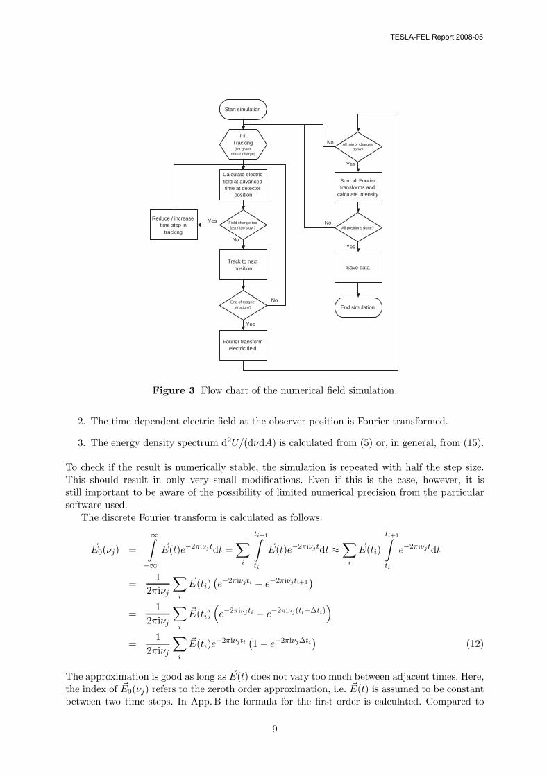
The numerical simulation is implemented in a straightforward manner, see the flow chart inFig. 3. The essential parts of the Matlab implementation are listed in App.D.

1. An electron is tracked through the known magnetic fields with a given step size. The electricfield strength at a given observation position at the future, advanced time given by thecurrent distance is calculated using (1a), see Fig. 4. Depending on the rate of change of thefield in observer time, the tracking step size is adapted. This approach avoids calculationof a retarded time, and allows to evaluate (3) easily.

8


Start simulation

InitTracking(for given

mirror charge)

Calculate electricfield at advancedtime at detector

position

Field change toofast / too slow?

Track to nextposition

End of magnetstructure?

Yes

No

Fourier transformelectric field

All mirror chargesdone?

Sum all Fouriertransforms and

calculate intensity

No

No

No

Reduce / increasetime step in

tracking

Yes

Yes

Yes

All positions done?

Save data

End simulation

Figure 3 Flow chart of the numerical field simulation.

2. The time dependent electric field at the observer position is Fourier transformed.

3. The energy density spectrum d2U/(dνdA) is calculated from (5) or, in general, from (15).

To check if the result is numerically stable, the simulation is repeated with half the step size.This should result in only very small modifications. Even if this is the case, however, it isstill important to be aware of the possibility of limited numerical precision from the particularsoftware used.

The discrete Fourier transform is calculated as follows.

�E0(νj) =

∞∫−∞

�E(t)e−2πiνjtdt =∑

i

ti+1∫ti

�E(t)e−2πiνjtdt ≈∑

i

�E(ti)

ti+1∫ti

e−2πiνjtdt

=1

2πiνj

∑i

�E(ti)(e−2πiνjti − e−2πiνjti+1

)=

12πiνj

∑i

�E(ti)(e−2πiνjti − e−2πiνj(ti+Δti)

)=

12πiνj

∑i

�E(ti)e−2πiνjti(1 − e−2πiνjΔti

)(12)

The approximation is good as long as �E(t) does not vary too much between adjacent times. Here,the index of �E0(νj) refers to the zeroth order approximation, i.e. �E(t) is assumed to be constantbetween two time steps. In App.B the formula for the first order is calculated. Compared to

9


z Position

Time

x P

ositi

on

Direction to Detector

Particle Track

Ele

ctric

Fie

ld a

t Det

ecto

r

Figure 4 Equidistant tracking steps naturally result in non-equidistant spacing of the electricfield during its peak due to the time compression from (3).

the implementation of (fast) Fourier transforms, this direct approach has the advantage of notrequiring equidistant time steps.5

An option is to use directly an expression for the electric field in frequency domain, forexample using a paraxial approximation for rapid computation [Gel05].

3.2 Comparison with analytic results

To check the correct behaviour of the numerical algorithm, its results for two of the analyticallysolved cases are presented in this section. The general parameters for the following calculationsare, as usual, those of a dipole from the first bunch compressor of FLASH.

3.2.1 Circular motion

Results for circular motion are compared in Fig. 5 with the frequency spectrum (6) for twoangles, Θ=0 and Θ=1/γ, and in Fig. 6 with the angular dependence. The agreement is verygood, being limited at low frequencies by the simulation time (the minimum frequency that canbe simulated is about the inverse of the simulation time, 2.3 · 109 Hz in this case) and at highfrequencies by the size of the time steps.

3.2.2 Long-wavelength edge radiation

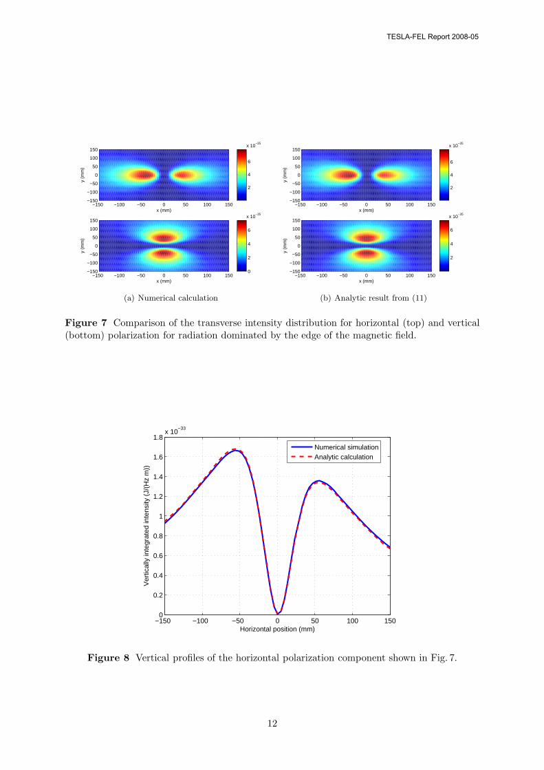
The transverse intensity distribution at 30 mm wavelength along the incoming beam direction at10 m distance as calculated numerically is shown in Fig. 7 together with an analytic calculationusing (11). The required condition for the validity of the analytic formula is fulfilled, and indeedthere is a very good agreement between the two distributions. At such long wavelengths, theedge effect dominates the emitted radiation characteristic. The deflection of the beam for theassumed field polarity is towards negative horizontal offsets.

The transverse distributions are indeed very similar, as can be seen in the vertically integratedprofiles of the horizontal polarization component shown in Fig. 8.

5To use an FFT algorithm, it would be necessary to resample �E(t) at high resolution with equidistant timesteps. The step width must be such that both �E(t) and e−2πiνt do not vary too much for all frequencies of interest.(12) also allows a different number of sample points for the frequency and time axis which is advantageous forfast varying time signals giving a comparatively broad, smooth frequency spectrum.

10


1010

1011

1012

1013

1014

1015

1016

10−38

10−37

10−36

10−35

10−34

10−33

Frequency (Hz)

Inte

nsity

(J/

(Hz

m2 ))

NumericAnalytic

1010

1011

1012

1013

1014

1015

1016

0.96

0.98

1

1.02

1.04

Frequency (Hz)

Ana

lytic

/ N

umer

ic

(a) Θ = 0

1010

1011

1012

1013

1014

1015

1016

10−38

10−37

10−36

10−35

10−34

Frequency (Hz)

Inte

nsity

(J/

(Hz

m2 ))

NumericAnalytic

1010

1011

1012

1013

1014

1015

1016

0.96

0.98

1

1.02

1.04

Frequency (Hz)

Ana

lytic

/ N

umer

ic

(b) Θ = 1/γ

Figure 5 Comparison of the frequency dependence of the numerical algorithm results with (6).The lower plot shows the ratio of analytical and numerical values.

−2 −1.5 −1 −0.5 0 0.5 1 1.5 20

0.5

1

1.5

2

2.5x 10

−36

y (m)

Inte

nsity

(J/

Hz

m2 )

NumericAnalytic

(a) 100 GHz

−0.2 −0.15 −0.1 −0.05 0 0.05 0.1 0.15 0.20

0.5

1

1.5

2

2.5

3

3.5x 10

−34

y (m)

Inte

nsity

(J/

Hz

m2 )

NumericAnalytic

(b) 300 THz

Figure 6 Comparison of the angular dependence of the numerical algorithm results with (6).

11


−150 −100 −50 0 50 100 150−150

−100

−50

0

50

100

150

x (mm)

y (m

m)

2

4

6

x 10−35

−150 −100 −50 0 50 100 150−150

−100

−50

0

50

100

150

x (mm)

y (m

m)

0

2

4

6

x 10−35

(a) Numerical calculation

−150 −100 −50 0 50 100 150−150

−100

−50

0

50

100

150

x (mm)

y (m

m)

2

4

6

x 10−35

−150 −100 −50 0 50 100 150−150

−100

−50

0

50

100

150

x (mm)y

(mm

)

2

4

6

x 10−35

(b) Analytic result from (11)

Figure 7 Comparison of the transverse intensity distribution for horizontal (top) and vertical(bottom) polarization for radiation dominated by the edge of the magnetic field.

−150 −100 −50 0 50 100 1500

0.2

0.4

0.6

0.8

1

1.2

1.4

1.6

1.8x 10

−33

Horizontal position (mm)

Ver

tical

ly in

tegr

ated

inte

nsity

(J/

(Hz

m))

Numerical simulationAnalytic calculation

Figure 8 Vertical profiles of the horizontal polarization component shown in Fig. 7.

12


1010

1011

1012

1013

1014

1015

1016

10−36

10−35

10−34

10−33

10−32

10−31

Frequency (Hz)

Inte

nsity

(J/

(m2 H

z))

Hard edge at t=0Hard edge at first zero crossingHard edge at both zero crossingsSoft edgeCircular motion

Figure 9 Radiation spectrum from a single dipole. For the hard edge cases, the observationpoint is tangentially to the trajectory at the edge, for the soft edge case slightly displaced in thebending direction. Circular motion is from (6).

3.3 Numerical results for a single magnet

Several peculiarities that occur in the spectra if only a magnet of finite length, especially withan edge, is considered can be seen in Fig. 9 in comparison to a spectrum resulting from circularmotion in a constant magnetic field. The observation point is tangentially to the trajectoryat 1 m distance from the entry edge. The hard edge, where the field jumps from 0 to 0.27 Tinstantaneously, is placed such that the acceleration term of the electric field in Fig. 2 is eithercut at t=0 or at the first zero crossing. In the former case, the time integral is still zero6 and thusthe spectrum drops towards long wavelength. The increased intensity at high frequencies is dueto the sharp edge that is introduced in the time-domain electric field. Although the field alreadyhas a very fast rate of change even for circular motion in the vicinity of the spike, an idealedge will of course imply even stronger Fourier components at high frequencies. In practice, bestuse of this effect requires placing the observation point within an angle better than 1/γ of theparticle direction at the magnetic edge, and an edge than rises or falls significantly faster thanthis. For the soft edge case, the actual dependence of the field on the z coordinate as measuredfor a bunch compressor dipole was used.

The maximum low-frequency intensity can be achieved if a magnet that bends the electronby an angle of 2γ is used, as this will cut the electric field in time-domain at its zero crossings,maximizing the integral (see Sec. 2.2.1 and Fig. 2). The achievable intensity in forward directioncan be calculated from the electric field (only the y component contributes):

Ey(ν = 0) =

∞∫−∞

Ey(t) dt = 2

Rβγc∫0

Ey(t′)1 + α2(t′)γ2

2γ2dt′

6The time integral over the electric field pulse from circular motion is zero. Due to the symmetry of the fieldwith respect to t = 0, this applies to either half of the field as well.

13


=2e

4πε0cL

1/γ∫0

β2 sin2 α − β cos α + β2 cos2 α

(1 − β cos α)31 + α2γ2

2γ2dα

=e

4πε0cLγ2

1/γ∫0

β − 1 + α2

2(1 − β + βα2

2

)3

(1 + α2γ2

)dα

=e

4πε0cLγ2

(2γ2

)2 1/γ∫0

α2γ2 − 1(α2γ2 + 1)2

dα

︸︷︷︸=−1/(2γ)

.

From (16), the energy per unit frequency per unit area becomes

d2U

dνdA(ν = 0) =

2μ0c

|Ey(ν = 0)|2 =e2γ2

2π2ε0cL2.

Interestingly, this is independent of the magnetic field itself, though the length of the magnethas to be chosen to give a bend of 2γ. For the parameters taken in Fig. 9, the zero frequencyintensity is 3.2 · 10−32 J/(m2Hz). The length of the radiation pulse in observer time is, from (8),twice the inverse of the critical angular frequency. For frequencies well below ωc, the term νtin the Fourier transform (4) is very small, the exponential close to unity, and consequently theintensity is independent on the frequency in this region.

3.4 Two magnets

Radiation from the exit of the second-last and from the entrance of the last dipole magnet ofthe first FLASH bunch compressor will interfere for the geometry of the synchrotron radiationport, as seen in the particle trajectory in Fig. 10. The resulting electric field and spectrum areshown in Fig. 11.7 The field in time domain shows two spikes of opposite sign and differentamplitude separated by Δt = 5 · 10−13 s. They result from the different bending direction anddifferent distance to the detector of the two magnets. The spectrum has a similar envelope as inthe case of circular motion, but overlaid with an oscillation with minima spaced in frequency by1/Δt = 2·1012 Hz. The integral over the field in time-domain is now nearly zero, so the spectrumdrops towards lower frequencies as for circular motion. The amplitude of the oscillation dependson the relative size of the two spikes in the time-domain electric field.

The interference of the radiation contribution from both magnets is also apparent in thetransverse intensity distribution, as seen in Fig. 12. The observation plane corresponds to theactual view port8, centered on the point indicated in Fig. 10. The top of the figure shows thedistribution if only the radiation from the last magnet is considered, the bottom the fine structurethat appears from the interference. It has to be kept in mind that these are single-electronspectra. The structures will be washed out if a bunch of finite size and divergence is considered.

3.5 Angular dependence of the spectrum

As was already seen in Fig. 5 for synchrotron radiation from circular motion, the spectrumdepends on the observation angle. This is shown for four angles in Fig. 13 for the case of two

7The random-like structures seen in the spectrum at high frequencies are an artifact of the limited number ofdiscrete frequencies for which the Fourier transform is calculated.

8The vacuum window is circular with 60 mm clear aperture, but the vertical dimension is determined by thevacuum chamber height.

14


−1.5 −1 −0.5 0 0.5

−0.4

−0.2

0

0.2

z (m)

x (m

)

D4BC2

D3BC2

Obs.

−1.5 −1 −0.5 0 0.5

−0.2

−0.1

0

0.1

0.2

0.3

z (m)

Mag

netic

fiel

d (T

)

Figure 10 Particle trajectory through the last two magnets of the first bunch compressorof FLASH and the magnetic field. An observation point on the vacuum chamber view port isindicated.

−5 −4 −3 −2 −1 0

x 10−13

−15

−10

−5

0

5

10

Time (s)

Ele

ctric

Fie

ld (

V/m

)

(a) Electric field

1010

1011

1012

1013

1014

1015

1016

10−37

10−36

10−35

10−34

10−33

10−32

10−31

Frequency (Hz)

Inte

nsity

(J/

(Hz

m2 ))

NumericAnalytic (B=0.26 T)

(b) Spectrum

Figure 11 Radiation pulse and spectrum from two magnets. The observation point is alongthe axis defined by the straight part of the trajectory between the dipoles shown in Fig. 10.

15


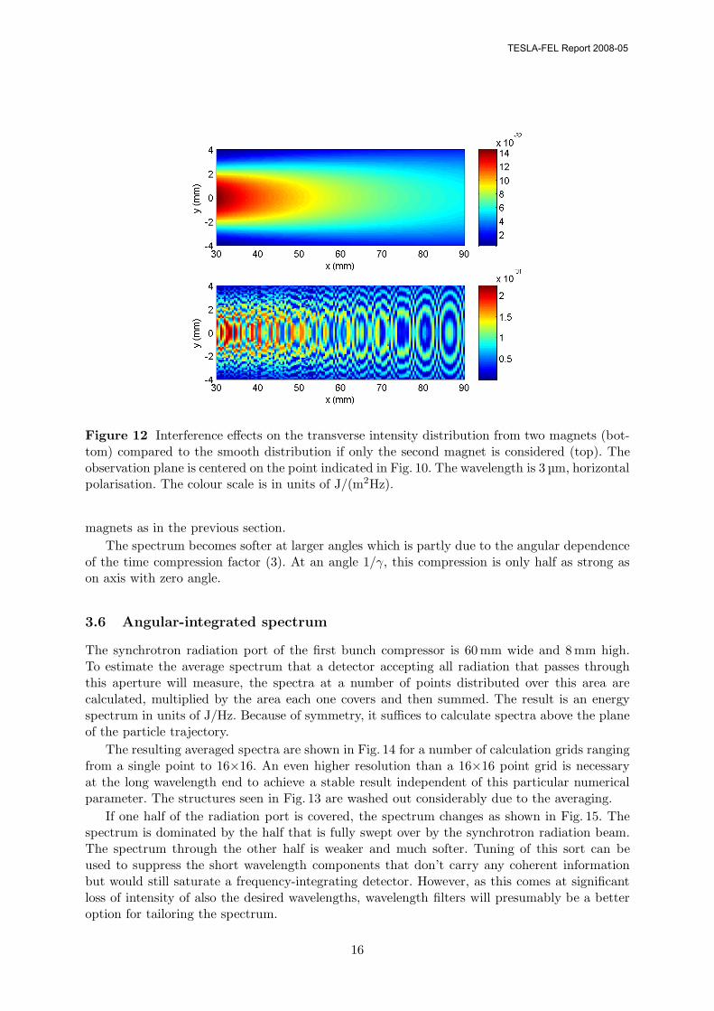
Figure 12 Interference effects on the transverse intensity distribution from two magnets (bot-tom) compared to the smooth distribution if only the second magnet is considered (top). Theobservation plane is centered on the point indicated in Fig. 10. The wavelength is 3 µm, horizontalpolarisation. The colour scale is in units of J/(m2Hz).

magnets as in the previous section.The spectrum becomes softer at larger angles which is partly due to the angular dependence

of the time compression factor (3). At an angle 1/γ, this compression is only half as strong ason axis with zero angle.

3.6 Angular-integrated spectrum

The synchrotron radiation port of the first bunch compressor is 60 mm wide and 8 mm high.To estimate the average spectrum that a detector accepting all radiation that passes throughthis aperture will measure, the spectra at a number of points distributed over this area arecalculated, multiplied by the area each one covers and then summed. The result is an energyspectrum in units of J/Hz. Because of symmetry, it suffices to calculate spectra above the planeof the particle trajectory.

The resulting averaged spectra are shown in Fig. 14 for a number of calculation grids rangingfrom a single point to 16×16. An even higher resolution than a 16×16 point grid is necessaryat the long wavelength end to achieve a stable result independent of this particular numericalparameter. The structures seen in Fig. 13 are washed out considerably due to the averaging.

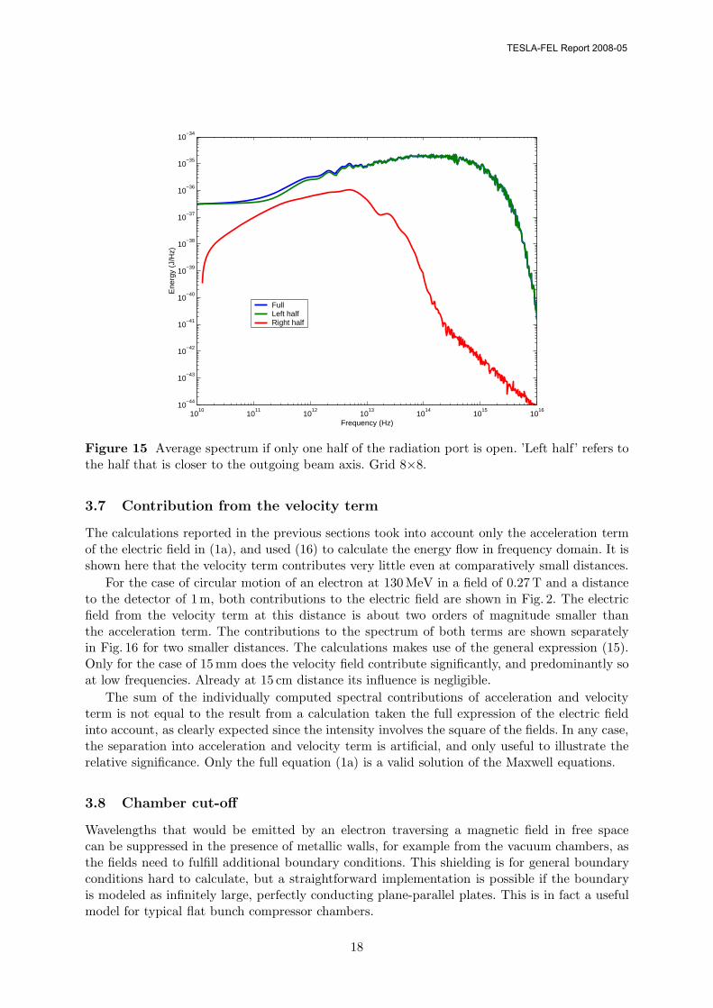
If one half of the radiation port is covered, the spectrum changes as shown in Fig. 15. Thespectrum is dominated by the half that is fully swept over by the synchrotron radiation beam.The spectrum through the other half is weaker and much softer. Tuning of this sort can beused to suppress the short wavelength components that don’t carry any coherent informationbut would still saturate a frequency-integrating detector. However, as this comes at significantloss of intensity of also the desired wavelengths, wavelength filters will presumably be a betteroption for tailoring the spectrum.

16


1010

1011

1012

1013

1014

1015

1016

10−36

10−35

10−34

10−33

10−32

10−31

Frequency (Hz)

Inte

nsity

(J/

(Hz

m2 ))

Θ=01/γ=3.9 mrad4/γ=15.7 mrad9/γ=35.4 mrad

Figure 13 Dependency of the spectrum on the observation angle Θ

1010

1011

1012

1013

1014

1015

1016

10−42

10−41

10−40

10−39

10−38

10−37

10−36

10−35

10−34

Frequency (Hz)

Ene

rgy

(J/H

z)

16x168x84x42x21x1

Figure 14 Dependency of the average spectrum on the calculation grid

17


1010

1011

1012

1013

1014

1015

1016

10−44

10−43

10−42

10−41

10−40

10−39

10−38

10−37

10−36

10−35

10−34

Frequency (Hz)

Ene

rgy

(J/H

z)

FullLeft halfRight half

Figure 15 Average spectrum if only one half of the radiation port is open. ’Left half’ refers tothe half that is closer to the outgoing beam axis. Grid 8×8.

3.7 Contribution from the velocity term

The calculations reported in the previous sections took into account only the acceleration termof the electric field in (1a), and used (16) to calculate the energy flow in frequency domain. It isshown here that the velocity term contributes very little even at comparatively small distances.

For the case of circular motion of an electron at 130 MeV in a field of 0.27 T and a distanceto the detector of 1m, both contributions to the electric field are shown in Fig. 2. The electricfield from the velocity term at this distance is about two orders of magnitude smaller thanthe acceleration term. The contributions to the spectrum of both terms are shown separatelyin Fig. 16 for two smaller distances. The calculations makes use of the general expression (15).Only for the case of 15 mm does the velocity field contribute significantly, and predominantly soat low frequencies. Already at 15 cm distance its influence is negligible.

The sum of the individually computed spectral contributions of acceleration and velocityterm is not equal to the result from a calculation taken the full expression of the electric fieldinto account, as clearly expected since the intensity involves the square of the fields. In any case,the separation into acceleration and velocity term is artificial, and only useful to illustrate therelative significance. Only the full equation (1a) is a valid solution of the Maxwell equations.

3.8 Chamber cut-off

Wavelengths that would be emitted by an electron traversing a magnetic field in free spacecan be suppressed in the presence of metallic walls, for example from the vacuum chambers, asthe fields need to fulfill additional boundary conditions. This shielding is for general boundaryconditions hard to calculate, but a straightforward implementation is possible if the boundaryis modeled as infinitely large, perfectly conducting plane-parallel plates. This is in fact a usefulmodel for typical flat bunch compressor chambers.

18


1011

1012

1013

1014

1015

1016

0

0.2

0.4

0.6

0.8

1

1.2

1.4

1.6

1.8

2

x 10−28

Frequency (Hz)

Inte

nsity

(J/

(m2 H

z))

Both termsAcceleration termVelocity term

(a) 15 mm

1011

1012

1013

1014

1015

1016

10−38

10−36

10−34

10−32

10−30

10−28

Frequency (Hz)

Inte

nsity

(J/

(m2 H

z))

Acceleration termVelocity term

(b) 15 cm

Figure 16 Comparison of spectral contribution of acceleration and velocity term for circularmotion for two distances. For better illustration, one vertical scale is linear, one is logarithmic.The radius of curvature is 1.6 m. In (b), the result with both terms is indistinguishable on thisscale from the acceleration term only.

Figure 17 Infinitely large, perfectly conducting planes (PEC) can be replaced by mirror chargesof alternating sign. Each charge emits synchrotron radiation into identical, finite cones, so onlya limited number will interfere on an observation point between the plates.

In this case, the walls, separated by distance h, can be replaced by mirror charges of alter-nating sign, placed at distance h from each other as depicted in Fig. 17. The mirror charges areoffset vertically from the actual charge, but otherwise are thought of as experiencing exactlythe same magnetic field and thus the same acceleration. Each of these charges has a matchingcharge of opposite sign opposite to either of the two planes, so clearly the condition of verticalelectric field on the boundaries is fulfilled.

The number of mirror charges that needs to be taken into account in practice is limitedby the finite opening angle of the radiation cone and the limited region between the planesover which the field needs to be calculated. For an infinite number of mirror charges, the fielddistribution repeats periodically in the vertical, but according to the model the field is sensiblydefined only between the plates.

19


1010

1011

1012

1013

1014

1015

0

0.2

0.4

0.6

0.8

1

1.2

1.4

Frequency (Hz)

Rel

ativ

e in

tens

ity

1000 mirror charges20 mirror chargesAnalytical calculation

Figure 18 Analytical [Dohl98] and numerical calculation of the chamber cut-off for circularmotion.

In [War90] a typical cut-off wavelength for electrons in circular motion with bending radiusR was determined as 2h

√h/R. For the first bunch compressor, with h=8mm, this cut-off is at

1.1 mm. For much shorter wavelengths the spectrum is unaffected, for much longer ones it iscompletely suppressed. Note, though, that again the condition of circular motion is in realitynot fulfilled.

In [Dohl98], a cut-off function is calculated (also for circular motion) as reproduced in Fig. 18for 10 m observation distance and the parameters of the first bunch compressor. The plot showsalso a comparison with a numerical calculation. The necessary number of mirror charges canbe estimated using the typical opening angle of synchrotron radiation in the far-infrared (10).On the observation plane at 10 m distance this gives a height of 2 m, and therefore the relevantnumber of mirror charges is a few times 2 m/8 mm=250. This is supported by the comparison,which perfectly reproduces the analytical interference structure resulting from the mirror chargesif 1000 such charges are considered, but fails for only 20.

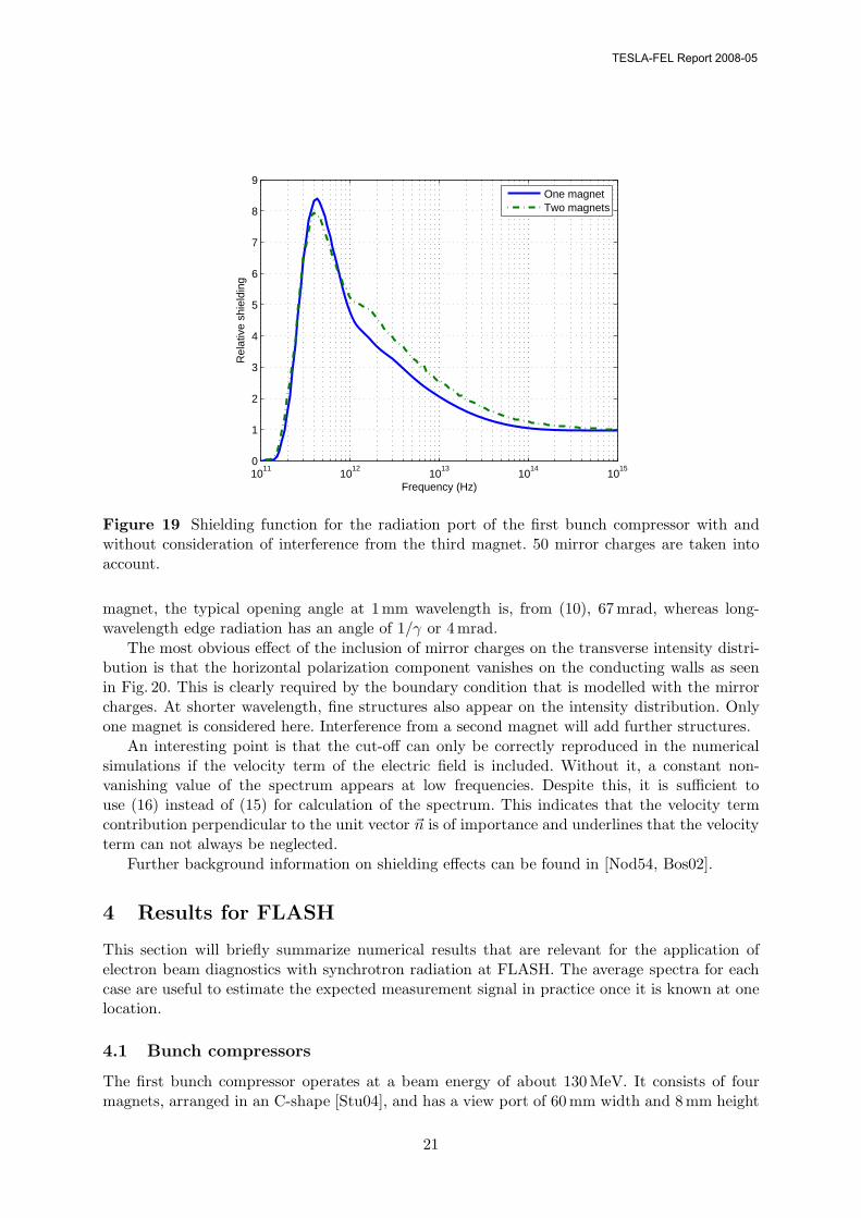
This requires a lot of computation time, as the simple implementation of the numericalcalculation tracks each mirror charge individually and then adds its electric field contribution infrequency domain at a particular observation point. The numerical simulation allows, however,to take into account a flat vacuum chamber for any magnetic field. This can result in verydifferent shielding behaviour than for circular motion, as seen in Fig. 19. The plot shows theratio of the average spectrum through the first bunch compressor view port (calculated witha high resolution of 128×128) with and without mirror charges, that is the shielding functionanalogous to Fig. 18. The shielding results in a concentration of energy close to the cut-off whichis much more pronounced than for circular motion. There is also some significant difference ifthe interference from the third magnet is included in the calculation as well.

The calculation presented in Fig. 19 includes 50 mirror charges above and below the bendingplane, although approximately 15 mirror charges are already enough to well reproduce the cut-offshape. This is very different than for circular motion, where many hundered mirror charges arenecessary. This reflects the much stronger collimation of radiation that is predominatly emittedfrom the edge of a magnetic field: for circular motion and the parameters of a bunch compressor

20


1011

1012

1013

1014

1015

0

1

2

3

4

5

6

7

8

9

Frequency (Hz)

Rel

ativ

e sh

ield

ing

One magnetTwo magnets

Figure 19 Shielding function for the radiation port of the first bunch compressor with andwithout consideration of interference from the third magnet. 50 mirror charges are taken intoaccount.

magnet, the typical opening angle at 1mm wavelength is, from (10), 67 mrad, whereas long-wavelength edge radiation has an angle of 1/γ or 4 mrad.

The most obvious effect of the inclusion of mirror charges on the transverse intensity distri-bution is that the horizontal polarization component vanishes on the conducting walls as seenin Fig. 20. This is clearly required by the boundary condition that is modelled with the mirrorcharges. At shorter wavelength, fine structures also appear on the intensity distribution. Onlyone magnet is considered here. Interference from a second magnet will add further structures.

An interesting point is that the cut-off can only be correctly reproduced in the numericalsimulations if the velocity term of the electric field is included. Without it, a constant non-vanishing value of the spectrum appears at low frequencies. Despite this, it is sufficient touse (16) instead of (15) for calculation of the spectrum. This indicates that the velocity termcontribution perpendicular to the unit vector �n is of importance and underlines that the velocityterm can not always be neglected.

Further background information on shielding effects can be found in [Nod54, Bos02].

4 Results for FLASH

This section will briefly summarize numerical results that are relevant for the application ofelectron beam diagnostics with synchrotron radiation at FLASH. The average spectra for eachcase are useful to estimate the expected measurement signal in practice once it is known at onelocation.

4.1 Bunch compressors

The first bunch compressor operates at a beam energy of about 130 MeV. It consists of fourmagnets, arranged in an C-shape [Stu04], and has a view port of 60 mm width and 8 mm height

21


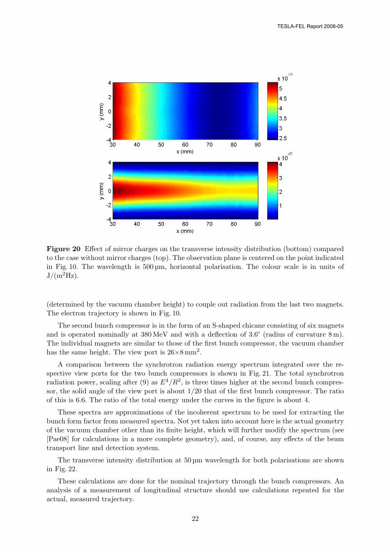
Figure 20 Effect of mirror charges on the transverse intensity distribution (bottom) comparedto the case without mirror charges (top). The observation plane is centered on the point indicatedin Fig. 10. The wavelength is 500 µm, horizontal polarisation. The colour scale is in units ofJ/(m2Hz).

(determined by the vacuum chamber height) to couple out radiation from the last two magnets.The electron trajectory is shown in Fig. 10.

The second bunch compressor is in the form of an S-shaped chicane consisting of six magnetsand is operated nominally at 380 MeV and with a deflection of 3.6° (radius of curvature 8 m).The individual magnets are similar to those of the first bunch compressor, the vacuum chamberhas the same height. The view port is 26×8 mm2.

A comparison between the synchrotron radiation energy spectrum integrated over the re-spective view ports for the two bunch compressors is shown in Fig. 21. The total synchrotronradiation power, scaling after (9) as E4/R2, is three times higher at the second bunch compres-sor, the solid angle of the view port is about 1/20 that of the first bunch compressor. The ratioof this is 6.6. The ratio of the total energy under the curves in the figure is about 4.

These spectra are approximations of the incoherent spectrum to be used for extracting thebunch form factor from measured spectra. Not yet taken into account here is the actual geometryof the vacuum chamber other than its finite height, which will further modify the spectrum (see[Pae08] for calculations in a more complete geometry), and, of course, any effects of the beamtransport line and detection system.

The transverse intensity distribution at 50 µm wavelength for both polarisations are shownin Fig. 22.

These calculations are done for the nominal trajectory through the bunch compressors. Ananalysis of a measurement of longitudinal structure should use calculations repeated for theactual, measured trajectory.

22


1011

1012

1013

1014

1015

1016

0

1

2

3

4

5

6x 10

−35

Frequency (Hz)

Inte

nsity

(J/

Hz)

First bunch compressorSecond bunch compressor

Figure 21 Single electron spectrum through the view ports of the first and second bunchcompressors (130 MeV/18° and 380 MeV/3.6°). 50 mirror charges and interference from last twodipole magnets taken into account.

(a) First bunch compressor (b) Second bunch compressor

Figure 22 Transverse intensity distribution on the view ports of both bunch compressors at50 µm. 50 mirror charges and interference from last two dipole magnets taken into account. Thecolour scale is in units of J/(m2Hz).

23


1011

1012

1013

1014

1015

1016

0.2

0.4

0.6

0.8

1

1.2

1.4

1.6

1.8x 10

−35

Frequency (Hz)

Inte

nsity

(J/

Hz)

40 45 50 55

−10

−8

−6

−4

−2

0

2

4

6

8

10

x (mm)

y (m

m)

2

4

6

8

10

12

x 10−32

Figure 23 Single electron spectrum without shielding integrated over the view port of thesecond energy collimator dipole and transverse intensity distribution at 10 THz. Energy 511 MeV.The colour scale is in units of J/(m2Hz).

4.2 Energy collimator

To remove off-energy electrons from the beam before passing the radiation-sensitive FEL undu-lators, an energy collimator is installed in FLASH. It consists of two dipole magnets, deflectingthe beam by nominally 3.5° in opposite directions, and so offsetting the beam horizontally by40 cm.

The second dipole has a small view port of 22 mm diameter. The spectrum, including inter-ference effects from the first dipole, passing this port at 511 MeV electron energy is shown inFig. 23, as well as the transverse intensity distribution at 10 THz. The interference is weak sincethe separation of the dipoles is 6.5 m. Mirror charges have not been considered, as the vacuumchamber has a height of 34 mm and suppression of the spectrum will only start at about 4 mmwavelength or 75 GHz frequency. The typical synchrotron radiation fan, starting about in themiddle of the view port, becomes apparent at higher frequencies.

4.3 Infrared undulator

The FLASH electromagnetic infrared undulator, installed after the FEL undulators, uses theelectron beam to generate pulses of radiation between 1 µm and 200 µm synchronized to the FELpulses. As undulator radiation is the result of synchrotron radiation emission from a periodicmagnetic structure, the single-electron emission spectrum of the undulator can be calculatedusing the numerical code presented here as well. However, the computation time becomes verylong when using the general time-domain approach.9 The results presented in this subsectionwere therefore calculated using the paraxial approximation from [Gel05], decreasing the com-putation time by more than two orders of magnitude. Beforehand, it was verified that there isagreement with the general approach for several points.

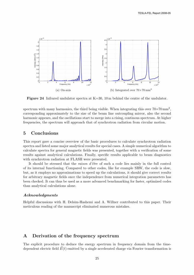
As the undulator has only 9 periods, the harmonics in the spectrum are relatively wide witha bandwidth of about 10%, and pronounced oscillations occur between the peaks, as can be seenin the on-axis spectrum in Fig. 24 calculated for a K value of 30, an electron energy of 511 MeV,and a distance of 10 m behind the centre of the undulator. The high K value results in a wiggler

9The reason is that the formation length is the full undulator, 4.3 m. The procedure to adapt the size of thetime steps and thus reduce computation time does not work efficiently in this case.

24


0 2 4 6 8 10 12

x 1012

0

0.2

0.4

0.6

0.8

1

1.2

1.4

1.6

1.8

2

x 10−32

Frequency (Hz)

Inte

nsity

(J/

(Hz

m2 ))

(a) On-axis

0 2 4 6 8 10 12

x 1012

0

0.5

1

1.5

2

2.5

3

3.5

4

4.5x 10

−35

Frequency (Hz)

Inte

nsity

(J/

Hz)

(b) Integrated over 70×70 mm2

Figure 24 Infrared undulator spectra at K=30, 10 m behind the centre of the undulator.

spectrum with many harmonics, the third being visible. When integrating this over 70×70mm2,corresponding approximately to the size of the beam line outcoupling mirror, also the secondharmonic appears, and the oscillations start to merge into a rising, continous spectrum. At higherfrequencies, the spectrum will approach that of synchrotron radiation from circular motion.

5 Conclusions

This report gave a concise overview of the basic procedures to calculate synchrotron radiationspectra and listed some major analytical results for special cases. A simple numerical algorithm tocalculate spectra for general magnetic fields was presented, together with a verification of someresults against analytical calculations. Finally, specific results applicable to beam diagnosticswith synchrotron radiation at FLASH were presented.

It should be stressed that the raison d’etre of such a code lies mainly in the full controlof its internal functioning. Compared to other codes, like for example SRW, the code is slow,but, as it employs no approximations to speed up the calculations, it should give correct resultsfor arbitrary magnetic fields once the independence from numerical integration parameters hasbeen checked. It can thus be used as a more advanced benchmarking for faster, optimized codesthan analytical calculations alone.

Acknowledgments

Helpful discussions with H. Delsim-Hashemi and A. Willner contributed to this paper. Theirmeticulous reading of the manuscript eliminated numerous mistakes.

A Derivation of the frequency spectrum

The explicit procedure to deduce the energy spectrum in frequency domain from the time-dependent electric field �E(t) emitted by a single accelerated charge via Fourier transformation is

25


shown here. To this end, first the straightforward time-domain expression for the Poynting vectorwill be deduced, then the corresponding frequency-domain expression and its interpretation.Finally, the energy flow for synchrotron radiation is calculated. All calculations are done for freespace, so the relative dielectric constant and permeability are taken as unity.

A.1 Poynting vector in time domain

The Maxwell equations in time domain are

�∇· �E(t) =1ε0

ρ(t), �∇× �E(t) = −∂ �B(t)∂t

,

�∇· �B(t) = 0, �∇× �B(t) = μ0�j (t) + ε0μ0∂ �E(t)

∂t,

(13)

where ρ(t) is the charge density and �j (t) the current density. The mechanical work per unit timeand volume done by the field on the charge density is given by �E(t)·�j (t), and can be expressedas

�E(t)·�j (t) =1μ0

�E(t) ·(

�∇× �B(t) − ε0μ0∂ �E(t)

∂t

)

=1μ0

[�B(t)·

(�∇× �E(t)

)− �∇·

(�E(t)× �B(t)

)− ε0μ0

�E(t)· ∂�E(t)∂t

]

=1μ0

[− �B(t)· ∂

�B(t)∂t

− �∇·(

�E(t)× �B(t))− ε0μ0

�E(t)· ∂�E(t)∂t

]

= − ∂

∂t

(�B2(t)2μ0

+ε0

�E2(t)2

)− 1

μ0

�∇·(

�E(t)× �B(t))

.

Integrating this over a volume V bounded by area A yields, through application of the divergencetheorem (assuming that there are no singularities within the volume), the Poynting theorem∫

V

�E(t)·�j (t)dV = − ∂

∂t

∫V

12μ0

�B2(t) +ε0

2�E2(t)︸︷︷︸

u(t)

dV −∮A

(1μ0

�E(t)× �B(t))

︸︷︷︸S(t)

·d �A.

The surface element d �A is normal to the surface. The left-hand side represents the total mechan-ical work per unit time done on the charges within V , allowing to identify the energy densityu(t) and the power flow �S(t), called the Poynting vector.

A.2 Poynting vector in frequency domain

Defining the Fourier transforms �E(ν), �B(ν), ρ(ν) and �j (ν) according to (4), and inserting into(13) yields the Maxwell equations in frequency domain. As an example,

�∇× �B(t) = �∇×∞∫

−∞

�B(ν)e2πiνt dν = μ0

∞∫−∞

�j (ν)e2πiνt dν + ε0μ0∂

∂t

∞∫−∞

�E(ν)e2πiνt dν.

Interchanging integration and differentiation yields∞∫

−∞

(�∇× �B(ν) − μ0�j (ν) − 2πiε0μ0ν �E(ν)

)e2πiνt dν = 0,

26


which has to hold for all t and therefore requires

�∇× �B(ν) = μ0�j (ν) + 2πiε0μ0ν �E(ν).

Similar for the other equations, yielding the set of Maxwell equations in frequency domain:

�∇· �E(ν) =1ε0

ρ(ν), �∇× �E(ν) = −2πiν �B(ν),

�∇· �B(ν) = 0, �∇× �B(ν) = μ0�j (ν) + 2πiε0μ0ν �E(ν).

Multiplying the rotation equation involving �E(ν) with − �B∗(ν)/μ0, taking the complex conjugaterotation equation involving �B(ν) and multiplying it with �E(ν), and then adding both results in

�E(ν) ·(

�∇× �B∗(ν))− �B∗(ν) ·

(�∇× �E(ν)

)= −�∇·

(�E(ν)× �B∗(ν)

)= 2πiν

(| �B(ν)|2 − ε0μ0| �E(ν)|2

)+ μ0

�E(ν)·�j ∗(ν).

Again through application of the divergence theorem, an integration over a volume V boundedby area A yields∫

V

�E(ν)·�j ∗(ν)dV = 2πiν∫V

ε0| �E(ν)|2 − 1μ0

| �B(ν)|2dV −∮A

(1μ0

�E(ν)× �B∗(ν))

︸︷︷︸S(ν)

·d �A,

defining the frequency-domain Poynting vector �S(ν).�S(ν) is a complex quantity, its significance with respect to energy transport is therefore

not immediately obvious. To clarify the connection, consider that the time-integrated time-domain Poynting vector must yield the same result as a suitably chosen quantity when frequencyintegrated. As frequencies should be non-negative, the relation can be deduced as follows:

∞∫−∞

�S(t) dt =1μ0

∞∫−∞

�E(t)× �B(t) dt =1μ0

∞∫−∞

∞∫−∞

�E(ν)e2πiνtdν×∞∫

−∞

�B(ν ′)e2πiν′tdν ′ dt

=1μ0

∞∫−∞

∞∫−∞

�E(ν)× �B(ν ′)∞∫

−∞e2πi(ν+ν′)tdtdνdν ′

=1μ0

∞∫−∞

�E(ν)× �B(ν ′)δ(ν + ν ′) dνdν ′

=1μ0

0∫−∞

�E(ν)× �B(−ν) dν +1μ0

∞∫0

�E(ν)× �B(−ν)dν

=1μ0

∞∫0

(�E(−ν)× �B(ν) + �E(ν)× �B(−ν)

)dν

=1μ0

∞∫0

(�E∗(ν)× �B(ν) + �E(ν)× �B∗(ν)

)dν by using (4)

27


=2μ0

∞∫0

�{

�E(ν)× �B∗(ν)}

dν = 2

∞∫0

�{

�S(ν)}

dν.

Twice the real part of the frequency-domain Poynting vector gives therefore the desired energyper unit area per unit frequency.

To illuminate the relation from a different side, consider a complex oscillating electric fieldE(t, ν) = �E(ν)e2πiνt, �E(ν) = Er(ν)+iEi(ν), Er(ν) and Ei(ν) real, and similarly for the magneticfield.10 A real time domain field is then, for example,

�E(t, ν) = �{E(t, ν)

}= �

{(Er + iEi)(cos 2πνt + i sin 2πνt)

}= Er(ν) cos 2πνt−Ei(ν) sin 2πνt.

The time-averaged time-domain Poynting vector for the electric and magnetic field thus definedis

�S(t) =1μ0

�E(t, ν)× �B(t, ν) =1

2μ0

(Er(ν) × Br(ν) + Ei(ν) × Bi(ν)

).

The real part of the frequency-domain Poynting vector is

�{�S(ν)} =1μ0

�{

(Er(ν) + iEi(ν)) × (Br(ν) + iBi(ν))}

=12

�S(t).

The real part of the complex frequency-domain Poynting vector is equal to half of the time-averaged time-domain Poynting vector.

A.3 Energy transport for synchrotron radiation

The energy that crosses an area dA per unit time, i.e. the power density d2U/(dtdA) at a certainposition is given by the absolute magnitude of the time-domain Poynting vector �S(t) deducedin Appendix A.1 above. Using the expression (1b) for the magnetic field from an acceleratedcharge, the Poynting vector becomes

�S(t) =1

μ0c�E(t)×

(�n(t′)× �E(t)

)= ε0c

(�E2(t)�n(t′) −

(�E(t)·�n(t′)

)�E(t)

),

where the retarded time t′ = t − R(t′)/c (see Sect. 2). Note that this fully general expressionassures that a stationary charge does not radiate, as then �E(t) and �n(t′) are constant and parallel,and the second term then cancels the first. Due to the retardation, they are still parallel for acharge in uniform motion, assuring also in this case that no energy is radiated.

If only the acceleration term of (1a) is considered (large distance from the source region),�E(t) and �n(t′) are perpendicular, thus in this case

d2U

dtdA=∣∣∣�S(t)

∣∣∣ = ε0c �E2(t). (14)

The units of this quantity are W/m2 = J/(s m2). The direction of power flow, given by thedirection of �S(t), is in general not along �n(t) except under this large distance condition.

The related quantity in frequency domain, the energy density spectrum dU/dν at a givenposition is, following the above calculations,

d2U

dνdA= 2

∣∣∣�{�S(ν)}∣∣∣ = 2

∣∣∣∣�{

1μ0

�E(ν)× �B∗(ν)}∣∣∣∣ . (15)

10These can essentially be though of as individual components of the inverse Fourier transform of (4).

28


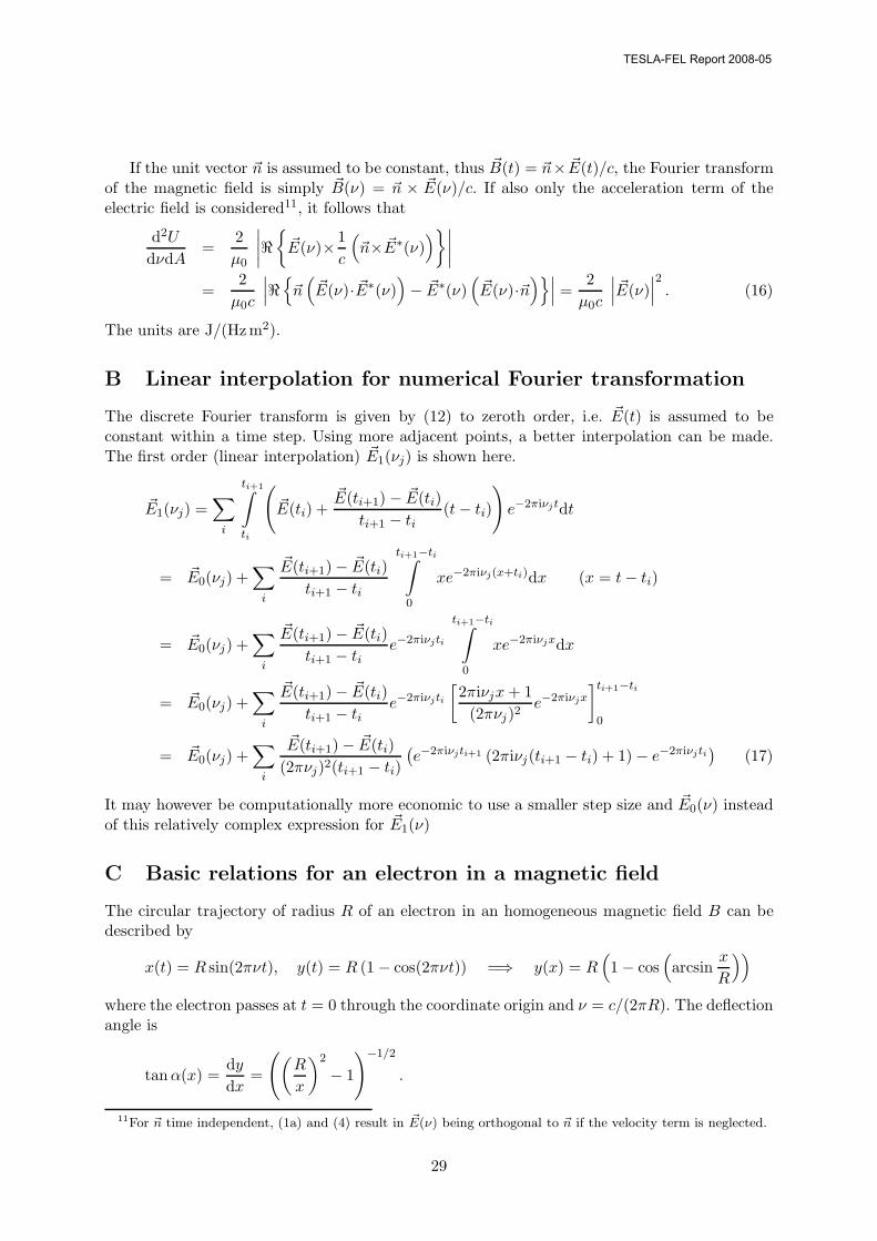
If the unit vector �n is assumed to be constant, thus �B(t) = �n× �E(t)/c, the Fourier transformof the magnetic field is simply �B(ν) = �n × �E(ν)/c. If also only the acceleration term of theelectric field is considered11, it follows that

d2U

dνdA=

2μ0

∣∣∣∣�{

�E(ν)× 1c

(�n× �E∗(ν)

)}∣∣∣∣=

2μ0c

∣∣∣�{�n(

�E(ν)· �E∗(ν))− �E∗(ν)

(�E(ν)·�n

)}∣∣∣ =2

μ0c

∣∣∣ �E(ν)∣∣∣2 . (16)

The units are J/(Hzm2).

B Linear interpolation for numerical Fourier transformation

The discrete Fourier transform is given by (12) to zeroth order, i.e. �E(t) is assumed to beconstant within a time step. Using more adjacent points, a better interpolation can be made.The first order (linear interpolation) �E1(νj) is shown here.

�E1(νj) =∑

i

ti+1∫ti

(�E(ti) +

�E(ti+1) − �E(ti)ti+1 − ti

(t − ti)

)e−2πiνjtdt

= �E0(νj) +∑

i

�E(ti+1) − �E(ti)ti+1 − ti

ti+1−ti∫0

xe−2πiνj(x+ti)dx (x = t − ti)

= �E0(νj) +∑

i

�E(ti+1) − �E(ti)ti+1 − ti

e−2πiνjti

ti+1−ti∫0

xe−2πiνjxdx

= �E0(νj) +∑

i

�E(ti+1) − �E(ti)ti+1 − ti

e−2πiνjti

[2πiνjx + 1

(2πνj)2e−2πiνjx

]ti+1−ti

0

= �E0(νj) +∑

i

�E(ti+1) − �E(ti)(2πνj)2(ti+1 − ti)

(e−2πiνjti+1 (2πiνj(ti+1 − ti) + 1) − e−2πiνjti

)(17)

It may however be computationally more economic to use a smaller step size and �E0(ν) insteadof this relatively complex expression for �E1(ν)

C Basic relations for an electron in a magnetic field

The circular trajectory of radius R of an electron in an homogeneous magnetic field B can bedescribed by

x(t) = R sin(2πνt), y(t) = R (1 − cos(2πνt)) =⇒ y(x) = R(1 − cos

(arcsin

x

R

))where the electron passes at t = 0 through the coordinate origin and ν = c/(2πR). The deflectionangle is

tan α(x) =dy

dx=

((R

x

)2

− 1

)−1/2

.

11For �n time independent, (1a) and (4) result in �E(ν) being orthogonal to �n if the velocity term is neglected.

29


For an electron energy E, the radius of curvature for relativistic energies (γ � 1) is

R =E

ecB=

mcγ

eB.

For a magnet with effective length l and a given angular deflection α

R = l

√1

tan2 α+ 1 (α < 90°).

The required magnetic field is

B =E

ecl

(1

tan2 α+ 1)−1/2

.

As examples, take the first bunch compressor at FLASH: E=130 MeV, l=50 cm, α=18° whichresults in B=0.27 T, R=1.6 m. For the second bunch compressor E=380 MeV, l=50 cm, α=3.6°giving B=0.16 T, R=8.0 m.

The instantaneous acceleration �β(t) = �v(t)/c of an electron by a magnetic field B(t) is giventhrough the Lorentz force as

�β(t) =e

mγ�β(t)× �B(t). (18)

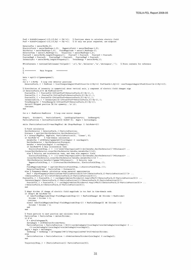
D Listing of the Matlab code

For reference, the essential parts of the SynchroSim Matlab code are listed here. It makes exten-sive use of matrix manipulations to take advantage of their fast computation. The full versionof the code has several cases of interest for FLASH implemented. As this requires an exter-nal magnetic field definition file, these are not reproduced here. The code is available from theauthor.

% Coordinate system as for FLASH, vectors are x y z. Particle trajectory is assumed

% flat (confined to x/z plane). All calculations are done in SI units.

clear; close all;

c0 = 2.99792458e8; m0 = 9.109389e-31;

e0 = -1.602177e-19; epsilon0 = 8.854187e-12;

CalcMode = 0; % 0 time-domain with acc. term, 1 full time-domain, 2 parax. approximation

SimulationCase = 0;

Frequency = logspace(10,16,200);

NumMirror = 50; % Number of mirror charges above orbit plane

Nx = 64; Ny = 64; % Point grid for calculation

deltat = 3.33e-12; % Set according to scale of magnetic field changes

MaxSteps = 200000; % Maximum number of steps for tracking (to avoid infinite loops)

MaxFieldChange = 1e-4; % Maximum change of electric field magnitude in V/m per step

MaxDivider = 64; % Maximum reduction factor of step size if field change too fast

% =========================================================================

% End user data section

% =========================================================================

load MagFieldDef.mat;

switch SimulationCase

case 0 % Circular motion with the viewport midpoint tangent to the arc at z=0

WidthX = 0.06; WidthY = 0.06; % Width and height of viewport

MidPoint = [0 0 1]; ViewportAngle = 0; % Centre position and rotation of viewport

B=0.27; gamma = 254.4; % 130 MeV

InitialAngle = pi/3; % Initial angle and position of particle trajectory

InitialPosition = -m0*c0/e0*gamma/B*[-(1-cos(InitialAngle)) 0 -sin(InitialAngle)];

MagZPos = [InitialPosition(3) -InitialPosition(3)]; MagField = [B B];

otherwise

disp ’Unknow simulation case, terminating...’;

return;

end

30


PosX = WidthX*linspace(-1/2,1/2,Nx) * (Nx~=1); % Positions where to calculate electric field

PosY = WidthY*linspace(-1/2,1/2,Ny) * (Ny~=1); % If only one point requested, use midpoint

DetectorPos = zeros(Nx*Ny,3);

ElectricField = zeros(MaxSteps-1,3); MagneticField = zeros(MaxSteps-1,3);

UnitVector = zeros(MaxSteps-1,3); FieldMagnitude = zeros(1,MaxSteps-1);

DetectorTime = zeros(1,MaxSteps-1); Trajectory = zeros(MaxSteps-1,2);

FourierX = zeros(Nx*Ny,length(Frequency)); FourierY = FourierX; FourierZ = FourierX;

FourierMagX = FourierX; FourierMagY = FourierX; FourierMagZ = FourierX;

IntensityAcc = zeros(Nx*Ny,length(Frequency)); TotalEnergy = zeros(Nx*Ny,1);

MFileContents = textread([mfilename(’fullpath’) ’.m’],’%s’,’delimiter’,’\n’,’whitespace’,’’); % Store contents for reference

%

% +++++++++++ Main Program +++++++++++

%

beta = sqrt(1-1/(gamma*gamma));

tic;

for k = 1:Nx*Ny % Loop over detector positions

DetectorPos(k,:) = MidPoint + [cos(ViewportAngle)*PosX(floor((k-1)/Ny)+1) PosY(mod(k-1,Ny)+1) -sin(ViewportAngle)*PosX(floor((k-1)/Ny)+1)];

% Distribution of intensity is symmetrical about vertical axis, y component of electric field changes sign

if DetectorPos(k,2)>0 && MidPoint(2)==0

FourierX(k,:) = FourierX(k-(2*find(PosY==DetectorPos(k,2))-Ny-1),:);

FourierY(k,:) = -FourierY(k-(2*find(PosY==DetectorPos(k,2))-Ny-1),:);

FourierZ(k,:) = FourierZ(k-(2*find(PosY==DetectorPos(k,2))-Ny-1),:);

IntensityAcc(k,:) = IntensityAcc(k-(2*find(PosY==DetectorPos(k,2))-Ny-1),:);

TotalEnergy(k) = TotalEnergy(k-(2*find(PosY==DetectorPos(k,2))-Ny-1));

fprintf(’Skipped position %d for symmetry...\n’,k);

continue;

end

for m = -NumMirror:NumMirror % Loop over mirror charges

Step=1; Divider=1; ParticleTime=0; LastDisplayTime=toc; IntEnergy=0;

ParticlePosition = InitialPosition+m*[0 WidthY 0]; Angle = InitialAngle;

while (ParticlePosition(3)<=max(MagZPos) && (Step<MaxSteps || CalcMode==2))

% Field calculation

UnitVecDetector = DetectorPos(k,:)-ParticlePosition;

Distance = sqrt(dot(UnitVecDetector,UnitVecDetector));

B = interp1(MagZPos, MagField, ParticlePosition(3), ’linear’, 0);

if CalcMode~=2 % Time-domain calculation

betaDotVec = e0*B*beta/(gamma*m0)*[cos(Angle) 0 -sin(Angle)];

UnitVecDetector = UnitVecDetector/Distance;

betaVec = beta*[sin(Angle) 0 cos(Angle)];

if CalcMode==0 % Only acceleration term

ElectricField(Step,:) = (-1)^m*e0/(4*pi*epsilon0*(1-dot(betaVec,UnitVecDetector))^3*Distance)* ...

(cross(UnitVecDetector,cross(UnitVecDetector-betaVec,betaDotVec))/c0);

else % Velocity and acceleration term, and then also magnetic field

ElectricField(Step,:) = (-1)^m*e0/(4*pi*epsilon0*(1-dot(betaVec,UnitVecDetector))^3*Distance)* ...

(cross(UnitVecDetector,cross(UnitVecDetector-betaVec,betaDotVec))/c0 + ...

(UnitVecDetector-betaVec)/(gamma^2*Distance)); % Velocity term

MagneticField(Step,:) = 1/c0*cross(UnitVecDetector, ElectricField(Step,:));

end

FieldMagnitude(Step) = sqrt(dot(ElectricField(Step,:),ElectricField(Step,:)));

DetectorTime(Step) = ParticleTime + Distance/c0;

else % Frequency-domain calculation using paraxial approximation

PhiT = 2*pi*Frequency*(ParticleTime-ParticlePosition(3)/c0+((DetectorPos(k,1)-ParticlePosition(1))^2+ ...

((DetectorPos(k,2))^2))/(2*c0*(DetectorPos(k,3)-ParticlePosition(3))));

FourierX(k,:) = FourierX(k,:) + cos(Angle)*deltat/Divider*c0.*exp(i*PhiT)/(DetectorPos(k,3)-ParticlePosition(3))* ...

(beta*sin(Angle)-(DetectorPos(k,1)-ParticlePosition(1))/(DetectorPos(k,3)-ParticlePosition(3)));

FourierY(k,:) = FourierY(k,:) + cos(Angle)*deltat/Divider*c0.*exp(i*PhiT)/(DetectorPos(k,3)-ParticlePosition(3))* ...

(-DetectorPos(k,2)/(DetectorPos(k,3)-ParticlePosition(3)));

end

% Adapt divider if change of electric field magnitude is too fast in time-domain mode.

if (Step>1 && CalcMode~=2)

if (abs(FieldMagnitude(Step)-FieldMagnitude(Step-1)) > MaxFieldChange) && (Divider < MaxDivider)

Divider = Divider * 2;

continue;

elseif (abs(FieldMagnitude(Step)-FieldMagnitude(Step-1)) < MaxFieldChange/2) && (Divider > 1)

Divider = Divider / 2;

end

end

% Track particle to next position and calculate total emitted energy

ParticleTime = ParticleTime + deltat/Divider;

if B~=0

R = m0*c0/e0*gamma/B;

deltaAngle = c0/R*deltat/Divider*beta;

ParticlePosition = ParticlePosition + R*[(1-cos(deltaAngle))*cos(Angle)+sin(deltaAngle)*sin(Angle) 0 ...

-(1-cos(deltaAngle))*sin(Angle)+sin(deltaAngle)*cos(Angle)];

Angle = Angle + deltaAngle;

IntEnergy = IntEnergy + e0^4*gamma^2*B^2/(6*pi*epsilon0*m0^2*c0)*deltat/Divider;

else

ParticlePosition = ParticlePosition + c0*deltat*beta/Divider*[sin(Angle) 0 cos(Angle)];

end

Trajectory(Step,:) = [ParticlePosition(1) ParticlePosition(3)];

31


Step = Step + 1;

end % Loop over particle trajectory

if Step==MaxSteps && CalcMode~=2

disp ’*** Attention: Simulation stopped by exceeding maximum number of steps ! ***’

return;

end

Step = Step - 1;

if CalcMode~=2

fprintf(1,’Calculating Fourier spectrum...\r’);

FourierX(k,:) = FourierX(k,:) + 1/(2*pi*i)./Frequency.*(ElectricField(1:Step-1,1).’*(exp(-2*pi*i*(DetectorTime(1:Step-1).’*Frequency)).* ...

(1-exp(-2*pi*i*(diff(DetectorTime(1:Step)).’*Frequency)))));

FourierY(k,:) = FourierY(k,:) + 1/(2*pi*i)./Frequency.*(ElectricField(1:Step-1,2).’*(exp(-2*pi*i*(DetectorTime(1:Step-1).’*Frequency)).* ...


FourierZ(k,:) = FourierZ(k,:) + 1/(2*pi*i)./Frequency.*(ElectricField(1:Step-1,3).’*(exp(-2*pi*i*(DetectorTime(1:Step-1).’*Frequency)).* ...


if CalcMode==1

FourierMagX(k,:) = FourierMagX(k,:) + 1/(2*pi*i)./Frequency.*(MagneticField(1:Step-1,1).’ ...

*(exp(-2*pi*i*(DetectorTime(1:Step-1).’*Frequency)).* (1-exp(-2*pi*i*(diff(DetectorTime(1:Step)).’*Frequency)))));

FourierMagY(k,:) = FourierMagY(k,:) + 1/(2*pi*i)./Frequency.*(MagneticField(1:Step-1,2).’ ...


FourierMagZ(k,:) = FourierMagZ(k,:) + 1/(2*pi*i)./Frequency.*(MagneticField(1:Step-1,3).’ ...


end

end

end % Loop over mirror charges

if CalcMode==2

FourierX(k,:) = -2*pi*i*Frequency*e0/c0^2.*FourierX(k,:)/(4*pi*epsilon0);

FourierY(k,:) = -2*pi*i*Frequency*e0/c0^2.*FourierY(k,:)/(4*pi*epsilon0);

Step = 2; % to avoid error from display commands below

else

TotalEnergy(k) = epsilon0*c0*dot(FieldMagnitude(1:Step-1).^2,diff(DetectorTime(1:Step)));

fprintf(’Total energy in time domain: %.4g J/m^2\n’, TotalEnergy(k));

end

if CalcMode==1

S = cross([FourierX(k,:);FourierY(k,:);FourierZ(k,:)],conj([FourierMagX(k,:);FourierMagY(k,:);FourierMagZ(k,:)]));

IntensityAcc(k,:) = 2*epsilon0*c0^2*sqrt(dot(real(S),real(S)));

else

IntensityAcc(k,:) = 2*epsilon0*c0*(abs(FourierX(k,:)).^2+abs(FourierY(k,:)).^2+abs(FourierZ(k,:)).^2);

end

if length(Frequency)>1

fprintf(’Total energy in frequency domain: %.4g J/m^2\n\n’, dot(IntensityAcc(k,1:length(Frequency)-1),diff(Frequency)));

end

fprintf(’Total emitted energy by electron: %.4g J\n’, IntEnergy);

end % Loop over detector positions

References

[Coı79] R. Coısson, Angular-spectral distribution and polarization of synchrotron radiationfrom a ‘short’ magnet, Phys. Rev. A Vol. 20, No. 2, 524 (1979)

[Chu93] O.V. Chubar, N.V. Smolyakov, Generation of intensive long-wavelength edge radi-ation in high-energy electron storage rings, Proceedings of the 15th IEEE ParticleAccelerator Conference, Washington D.C., 17-20 May 1993, pp. 1626-1628

[Dohl98] M. Dohlus, T. Limberg, Calculation of synchrotron radiation in the TTF-FEL bunchcompressor magnet chicanes, Nucl. Instr. Meth. A 407, 278 (1998)

[Gel03] G. Geloni et al., A method for ultrashort electron pulse-shape measurements usingcoherent synchrotron radiation, DESY 03-031 (March 2003)

[Gel05] G. Geloni et al., Paraxial Green’s function in synchrotron radiation theory, DESY05-032 (February 2005)

[Gri06] O. Grimm, P. Schmuser, Principles of coherent radiation diagnostics, TESLA FEL2006-03 (2006)

[Sal97] E.L. Saldin et al., On the coherent radiation of an electron bunch moving in an arcof a circle, Nucl. Instr. Meth. A 398, 373 (1997)

32


[Jack75] J.D. Jackson, Classical Electrodynamics, John Wiley & Sons, New York (1975)

[Meot99] F. Meot, A theory of low frequency far-field synchrotron radiation, Part. Accel. 62,215 (1999)

[Pae08] A. Paech, Evaluation numerischer Methoden zur Berechnung von Synchrotron-strahlung am ersten Bunchkompressor des Freie-Elektronen-Lasers FLASH, PhDthesis Technische Universitat Darmstadt, February 2008

[Nod54] J.S. Nodvick, D.S. Saxon,Suppression of coherent radiation by electrons in a syn-chrotron, Phys. Rev. 96, 180 (1954)

[Bos02] R.A. Bosch, Shielding of infrared edge and synchrotron radiation, Nucl. Instr. Meth.A 482, 789 (2002)

[War90] R. L. Warnock, Shielded coherent synchrotron radiation and its effect on very shortbunches, SLAC-PUB 5375 (November 1990)

[Stu04] F. Stulle, A Bunch Compressor for small Emittances and high Peak Currents at theVUV Free-Electron Laser, PhD thesis Universitat Hamburg, August 2004

33


synchrotron radiation for beam diagnostics: numerical ... · synchrotron radiation for beam...

Documents