synergy of airborne lidar data and vhr satellite optical - itc

Synergy of Airborne LiDAR data and VHR Satellite Optical Imagery

for Individual Crown and Tree Species Identification

COLLINS BYOBONA KUKUNDA MAY, 2013

ii

Course Title: Geo-Information Science and Earth Observation for Environmental Modelling and Management

Level: Master of Science (MSc) Course Duration: August 2011 – June 2013 Consortium Partners:

Lund University, (Sweden) University of Twente,

Faculty ITC (The Netherlands) University of Southampton, (UK) University of Warsaw, (Poland) University of Iceland, (Iceland)

University of Sydney, (Australia, Associate partner)

iii

Synergy of Airborne LiDAR Data and VHR Satellite Optical Imagery for

Individual Crown and Tree Species Identification

By

COLLINS BYOBONA KUKUNDA Thesis submitted to Faculty of Geo-Information Science and Earth Observation of the University of Twente in partial fulfilment of the requirements for the degree of Master of Science in Geo-information Science and Earth Observation, Specialisation: Environmental Modelling and Management. Thesis Assessment Board Prof. dr. A. K. Skidmore (Chair) Dr. ir. S. J. Oude Elberink (External Examiner, Department of Earth Observation Science, ITC) Dr. Y. A. Hussin (First Supervisor) Dr. H. A. M. J. van Gils (Second Supervisor)

iv

Disclaimer

This document describes work undertaken as part of a programme of study at the Faculty of Geo-Information Science and Earth Observation of the University of Twente. All views and opinions expressed therein remain the sole responsibility of the author, and do not necessarily represent those of the Faculty.

v

Abstract Accurate data on individual tree crowns and their species within stands is still limited affecting many remote sensing studies on allometric equations, timber volume, above ground biomass and carbon exchange. This study evaluated the synergistic use of fine resolution multispectral imagery (WorldView-2, 2 m) and high density LiDAR data (160 points/m-2) for individual crown segmentation and species identification and classification of two conifer species (Scots Pine-Pinus sylvestris L. and Mountain pine-Pinus uncinata Mill. Ex Mirb) in a mountainous area of the southern French Alps. The integration of WorldView-2 multispectral imagery and LiDAR data was considered during image segmentation and subsequent species identification and classification on a premise of complementarity. Three individual crown segmentation and species identification schemes were examined namely; segmentation and species identification based on LiDAR layers, spectral layers and a combination of the two datasets. A region growing segmentation approach was used. For each scheme, individual treetops were identified using a fixed-window local maxima approach and were used as seed pixels to grow individual tree crowns. The individual crown segments were subsequently used to derive one spectral and three physical parameters for species identification and classification. Tree height, crown diameter and the coefficient of variation of LiDAR intensity were the physical parameters derived from LiDAR data whereas the maximum WorldView-2 satellite albedo reflectance was the spectral attribute derived from the optical satellite data. Logistic Regression and Classification and Regression Trees (CART) modelling approaches were used to identify each tree to either Scots or Mountain pine. Quantitative segmentation quality assessment showed that the LiDAR derived segments were superior (Segmentation goodness = 86.4%) to the optical segments. However, given the distortions in the multispectral image, integration of the datasets for individual crown segmentation was not possible. Classification accuracy results showed that the integration of spectral and LiDAR data improved the species identification and classification compared to using either data sources independently. The highest classification accuracy (Kappa = 54%) was acquired when using both spectral and LiDAR derived metrics and a CART approach. This study concluded that although the integration of LiDAR and WorldView-2 was not possible to achieve for this study, it is still conceptually feasible and that the integration of the datasets for individual tree species identification and classification using a regression modelling approach provided increased interpretation capabilities and an opportunity for more reliable results.

vi

Acknowledgements First of all, I would like to thank God for guiding me right from the point I started on the GEM course in August 2011. Many milestones have been turned, wonderful people met, beautiful places seen, various perspectives developed, valuable knowledge earned and the future made brighter. Only God could have made this possible for me. Secondly, I would like to express my heartfelt appreciation to my supervisors for their invaluable guidance and encouragement throughout the thesis period. My sincere gratitude goes to my primary supervisor Dr. Y. A. Hussin who introduced this wonderful research topic to me. The responsibility you entrusted me forced me to take action and develop. Thank you for the fruitful discussions and reviews during the project period. Secondly, I am grateful to my second supervisor Dr. H. A. M. J. van Gils for his motivation and critical criticism. You always had confidence in me and my work which stimulated me to work harder at every stage of this research. The discussions I had with you gave me real insight into the study. I must specifically express my sincere gratitude to both of you (my supervisors) for accompanying me to the field to trek the French Alps and share joyful moments while working. I would like to thank the European Union Erasmus Mundus GEM scholarship program for funding my studies and stay in Europe. It has been a great opportunity to improve my skills, experiences and qualifications on this course and I feel greatly indebted. The opportunity to study at Lund University, Sweden and the University of Twente, Netherlands was life changing. I had an amazing multicultural experience. Special acknowledgement goes to Ms. A. Khosravipour, on whose PhD project I worked. Thank you for allowing me to contribute to your project and for being a friend that stood by me all through the thick-and-thin. My sincere gratitude is directed specifically your contribution and guidance regarding the research structure, analysis and thesis preparation. Your cautious yet friendly spirit kept me on the right track. May the almighty God richly bless you. To all my friends, what would I have done without your moral, academic and spiritual support? I am indebted to your loyalty and pledge to preserve it. My lovely family especially my parents and my brothers Isaac Mwesigwa and Lt. Martin Atuhaire (RIP), Auntie Abooki and family, Grandma, Uncles and Aunties, I cannot thank you enough for your prayers and support, you forever remain close to my heart.

vii

Table of Contents Abstract .................................................................................. vAcknowledgements ................................................................... viList of figures ........................................................................... ixList of tables ............................................................................ xi Chapter 1 ................................................................................ 1

1.1 INTRODUCTION ................................................................ 11.1.1 Background ................................................................ 11.1.2 Segmenting Individual Tree Crowns ............................... 31.1.3 Identification of Tree Species ........................................ 51.1.4 Overview of LiDAR Technology ...................................... 71.1.5 Overview of WorldView-2 Optical Imagery ...................... 91.1.6 Problem Statement .................................................... 101.1.7 General Objective....................................................... 131.1.8 Specific Objectives ..................................................... 131.1.9 Research Questions .................................................... 131.1.10 Research Hypotheses ................................................ 141.1.11 Thesis Outline .......................................................... 14

Chapter 2 ............................................................................... 17

2.1 STUDY AREA, MATERIALS AND METHODS ........................... 172.1.1 Study Area ................................................................ 172.1.2 Materials ................................................................... 212.1.2 Methods.................................................................... 23

Chapter 3 ............................................................................... 43

3.1 RESULTS ........................................................................ 433.1.1 Forest Condition ......................................................... 433.1.2 Individual Tree Detection ............................................ 453.1.3 Tree physical parameters ............................................ 493.1.4 Crown spectral parameter ........................................... 503.1.5 Regression modelling .................................................. 54

Chapter 4 ............................................................................... 57

4.1 DISCUSSION .................................................................. 574.1.1 Field Methods ............................................................ 574.1.2 Forest Condition ......................................................... 584.1.3 Geometric co-registration of datasets ............................ 584.1.4 Treetop Identification.................................................. 594.1.5 Crown segmentation ................................................... 624.1.6 Tree physical parameters ............................................ 634.1.7 Crown spectral parameter ........................................... 644.1.8 Tree species identification ........................................... 64

viii

Chapter 5 ............................................................................... 675.1 CONCLUSION AND RECOMMENDATIONS ............................. 67

5.1.1 Conclusion ................................................................ 675.1.2 Recommendations ...................................................... 68

References .............................................................................. 71Appendices ............................................................................. 81

ix

List of Figures Figure 1: Understanding LiDAR systems and Returns (t stands for Time, I stands for Intensity) Source: (USGS, 2013) ....................... 8Figure 2: WorldView-2 Bands ..................................................... 9Figure 3: Position of House in the images (Left: WV2 Right: LiDAR CHM Below: ortho-photo) before co-registration ........................... 12Figure 4: Shadows of Trees (Highlighted by arrow in bottom Right) 12Figure 5: RGB Orthophoto of the study area within France (Inset). . 18Figure 6: Cones of Scots and Mountain pine................................. 21Figure 7: Workflow for Objective One ......................................... 23Figure 8: Workflow for Objective Two ......................................... 24Figure 9: Bios Noir Land Cover map ........................................... 25Figure 10: Sampling layout ....................................................... 26Figure 11: Top Left: DSM, Top Right: DTM, Bottom Left: CHM viewed in 2D, Bottom Right: CHM viewed in 3D ...................................... 32Figure 12: Left: un-normalized LiDAR point cloud, Right: normalized LiDAR point cloud .................................................................... 33Figure 13: Left: DIM, Right: Ortho-photo (Showing the same position on ground) ............................................................................. 33Figure 14: A 3D view of the panchromatic band (Left) and the CHM (Right) over the same area. ...................................................... 34Figure 15: Boxplots of field measurements .................................. 43Figure 16: Correlation between DBH and Height, DBH and Crown Diameter Top: Scots pine. Bottom: Mountain pine. ....................... 44Figure 17: Spatial profile or surface contour of plots. .................... 45Figure 18: Spatial profile or surface contour of plots (Spectral Bands 1-8). ...................................................................................... 46Figure 19: Gap Masks ............................................................... 46Figure 20: Automatically detected treetops. Left: WorldView-2. Right: LiDAR CHM. Inset: Visualized area highlighted in white ................. 47Figure 21: Segmentation results. Left: LiDAR. Right: WorldView-2 .. 48Figure 22: LiDAR derived Tree Height (Top) and Crown diameter (Bottom). Height with outliers (left), Height without outliers (Right), Crown diameter using a circular model (Left), Crown diameter using an elliptic model (Right) ............................................................ 49Figure 23: Intensity Standard Deviation (SD) and Coefficient of Variation (CoV) of the two pine species ....................................... 50Figure 24: Maximum WorldView-2 DN values per crown and between species. .................................................................................. 51Figure 25: Within crown statistics of WorldView-2 Band 678 composite between species ....................................................... 52Figure 26: Within crown WorldView-2 satellite albedo statistics between species ...................................................................... 53Figure 27: WorldView-2 spectral profiles of the two tree species ..... 54

x

Figure 28: Model accuracy results .............................................. 55Figure 29: Species classification maps. ....................................... 56Figure 30: Topographic distortions. Left: WorldView-2 Image after geometric correction. Right: WorldView-2 Image before geometric correction. .............................................................................. 59Figure 31: Automatically detected treetops from WorldView-2 panchromatic image ................................................................. 60

xi

List of Tables Table 1: Classification specifications for LAS 1.0 & LAS 1.2 formats .. 9Table 2: LiDAR Meta data .......................................................... 22Table 3: Correlation across WorldView–2 bands (Highlighted are the lowest correlation values) ......................................................... 29Table 4: Ortho-rectification Tie points ......................................... 30Table 5: Accuracy of automatically detected treetop (Highlighted are the top three accuracies obtained). Buffer refers to search window size. ...................................................................................... 47Table 6: Variance Inflation Factors across explanatory variables ..... 55

1

Chapter 1

1.1 INTRODUCTION

1.1.1 Background Forests are important earth resources providing both ecosystem products and services (FAO, 2012). For this reason, forests require to be sustainably managed. However, if sustainable management of forests for purposes such as commercial logging, biodiversity management or for meeting wildlife, environmental and recreational goals is to be achieved, forests must be inventoried. Inventory has for long been a common practise for good forest management however, in the recent past, studies on inventory and improved forest management have particularly gained wider attention with the appreciation of global climatic change concepts and development of forest-centred climate change mitigation strategies (Nabuurs, 2007). For example, various developing countries will soon be seeking carbon financing for protecting their forests as part of the evolving (United Nations Framework Convention on Climate Change-Reducing Emissions from Deforestation Degradation) UNFCCC REDD+ negotiations. As a prerequisite to successful baseline, monitoring and accounting of these projects; the UNFCCC expects all REDD+ stakeholders to use methodologies that estimate emissions and removals in a demonstrable, as accurate as possible, complete, comparable, verifiable, and with consistence as stipulated in the Vienna convention for the protection of the ozone layer and the Montreal protocol on substances that deplete the ozone layer (UNEP, 2000). With initiatives such as this, it is clear that forest inventory will remain a core aspect of forest monitoring and management. Therefore techniques that automate the inventory procedures and provide optimally accurate estimates will gain significance. There are different techniques of forest inventory. Traditionally, forest inventory was solely field-plot based but later emerged the manual aerial photographic interpretation of high resolution forest cover data. Then begun analysis of high resolution satellite imagery data and more recently, analysis of terrestrial and airborne photogrammetry data (Tomppo, 2009). Despite this evolution, all techniques aim at extraction of forest variables such as Diameter at Breast Height (DBH), tree density, basal area, tree height, stand volume, species

Introduction

2

dominance, species composition, species diversity etc. (Kaartinen et al., 2012) aiming at improving the understanding of the forests’ growth structures and composition. Although a very useful forest inventory variable like DBH is still difficult to extract from airborne or spaceborne data (Dalponte et al., 2011; Bi et al., 2012), the future points to domination of remote sensing techniques in forest inventory. This is mainly because; (1) remote sensing techniques provide higher accuracies in prediction of many forest variables, (2) data derived is easy to extrapolate over large areas since they are not dependent on stand boundaries, (3) the techniques can be used to relative accuracy in areas of limited access such as mountainous and dense forests (4) data acquisition and processing costs are less and (5) the ability to extract forest resource maps key in forest management (Wang et al., 2004; Tomppo, 2009; Véga & Durrieu, 2011; Kaartinen et al., 2012). The issue of the prediction accuracies often arises in remote sensing studies on forest inventory. Theoretically, forest attributes can be estimated at higher accuracies if remote sensing techniques are integrated than used in isolation. This is because use of multi-sensoral data together with improved integration methods may overcome some of the problems which are faced with single data sets (Koch, 2010). Leckie et al. (2003) demonstrate that Light Detection and Ranging (LiDAR) and high resolution optical imagery indeed complement each other while mapping crowns of individual trees in both open and closed temperate forest stands. They achieved 80%–90% good correspondence with the ground reference tree delineations based on ground data. Shreuder et al. (2008) used an empirical analysis of LiDAR intensity data and found out that this data alone could distinguish broadleaved species from conifers and further distinguish various tree species within these broad groups with classification accuracies ranging between 70%-98%. On the other hand, Sugumaran and Voss (2007), utilized the LiDAR intensity data in integration with high resolution multispectral and hyper-spectral data to create image segments and user defined class rules and found that fusing LiDAR data with optical imageries enhanced the classification accuracies by 10%. Holmgren et al. (2008) combined LiDAR data with optical imagery for individual-tree-based species identification and presented the benefits of integrating very high resolution LiDAR data and high spatial resolution aerial imagery. Straub et al. (2009) and Popescu (2004) provide examples of research which utilized the combination of tree structural features from LiDAR with spectral information of multispectral image to improve biomass and volume estimates. Heinzel and Koch (2012) also investigated comprehensive sets of different types of features

Chapter 1

3

which were derived from LiDAR height metrics, texture, hyperspectral data and color infrared for classifying four tree species. Kim et al. (2010) used fusion of aerial photography and LiDAR data for delineation of individual trees to improve carbon storage estimates. The aforementioned examples provide practical context to possible synergies between LiDAR and fine resolution optical imagery. The general idea in this study is that while LiDAR offers high geometric detail (peaks and valleys) to explain the height, structure and size of individual tree canopies (Chen et al., 2006), the lack of spectral signature remains an important limitation of this data in forest inventory studies (Leckie et al., 2003; Lim et al., 2003; Deng et al., 2007; Suratno et al., 2009b; Swatantran et al., 2011). Consequently, foresters continue to rely on field survey and a priori knowledge of vegetation distributions and to some extent passive remote sensing to generate species data (Cho et al., 2011). Therefore, by utilizing LiDAR vertical structural and intensity data as well as the optical imagery spectral data, output accuracies for individual tree crown segmentation and species identification may improve.

1.1.2 Segmenting Individual Tree Crowns Segmentation of individual trees and extraction of relevant tree structure information from remotely sensed data is very useful in a variety of forest applications (Chen et al., 2006). For example, to estimate the stem volume, segmenting individual tree crowns and extracting relevant tree structure parameters is prerequisite (Erikson, 2004). To obtain such individual tree parameters, the initial process is to isolate individual trees and delineate tree crown boundaries. Measuring precise crown segmentation is a challenging task, because the irregularity of many crown shapes is difficult to capture using standard forestry field equipment (Kato et al., 2009). Therefore, intensive research has been done on automated tree detection and crown delineation using remotely sensed data. Earlier remotely sensed data from space are not suitable for tree crown segmentation because the pixel size is usually much larger than a typical tree crown size. Strahler (1986) referred to spatial resolution of these images with respect to object size as low-resolution. Due to the limitation in pixel resolution of earlier remote sensing data from space, a significant amount of work extracting tree crown size was based on high spatial resolution aerial photos (Brandtberg & Walter, 1998). Pitt et al. (1997) concluded that only the very high-resolution capabilities of aerial photography and digital cameras would be suitable. Automatic tree crown detection from

Introduction

4

aerial photos requires the pixel size to be much smaller than the tree crown size in order to define tree crown boundaries. However, high spatial resolution increases variation in within-crown brightness, making tree crown identification difficult (Song et al., 2010). Automatic detection often assumes that each tree has a distinct boundary with no overlap between adjacent crowns, but such overlap is common. Therefore, validation shows that direct delineation of tree crowns on high spatial resolution aerial photos can lead to significant errors in both the number of crowns and the crown size on a tree-by-tree basis (Brandtberg & Walter, 1998). With the emergence of very high spatial resolution satellite images such as IKONOS and QuickBird, the pixel and spectral resolution gap which existed between satellite images and aerial photographs has decreased (Carleer & Wolff, 2004). They commend a more object-oriented image analysis paradigm, one that shift from pixel-based techniques towards the delineation of individual tree crowns (Gougeon & Leckie, 2006). The object-oriented approach will reduce the local spectral variation caused by crown textures, gaps and shadows. In addition, any type of spatially distributed data such as elevation, intensity and population density can be used as input to image segmentation to produce image objects (Ke et al., 2010). Moreover, to detect and delineate individual tree crowns several algorithms can be applied on imagery including, the valley- following (Gougeon, 1995), edge detection using scale-space theory (Brandtberg and Walter, 1998), template matching (Pollock, 1996), local transect analysis (Pouliot et al., 2002), watershed segmentation (Wang et al., 2004), local maxima filtering with fixed or variable window sizes (Wulder et al., 2000), 3D modelling (Gong et al., 2002), marker-controlled watershed segmentation (Meyer & Beucher, 1990). These algorithms are mostly based on the assumption that there are “peaks” of reflectance around the treetops and “valleys” along the canopy edges. However, the “peaks” and “valleys” are not always distinct since canopy reflectance is affected by various factors such as illumination conditions, canopy spectral properties, and complex canopy structure (Chen et al., 2006). Palace et al. (2008) developed an automatic tree crown detection and delineation algorithm using IKONOS image, and found that the automatic algorithm was not able to detect understory trees and overestimated the size and frequency of large trees. Wulder et al. (2004) compared an IKONOS image with an airborne image collected at the same spatial resolution and found that the 1 m panchromatic IKONOS image can be used to identify 85% of tree crowns, but with a 51% commission error.

Chapter 1

5

Recently, researchers have begun to apply LiDAR data in individual tree isolation crown extraction (Persson et al., 2002). Compared with passive imaging, LiDAR has the advantage of directly measuring the three-dimensional coordinates of canopies. Therefore, the geometric, rather than spectral, “peaks” and “valleys” can be detected (Chen etal., 2006). Several studies have extended methods developed for optical imagery and aerial photos into LiDAR data for tree detection (Hyyppa et al., 2001; Koch et al., 2006). Brandtberg et al. (2003) extended the scale-space theory to detect individual crown segments. Chen et al. (2006) applied the marker-controlled watershed segmentation into LiDAR data to avoid the over-segmentation problems. However, the studies have shown that over-estimation problems remain (Kim et al., 2010). Nevertheless, a few studies have tried to combine fine resolution optical imagery with LiDAR data for crown segmentation. In theory, a major limitation of the automated tree detection of spectral imagery has been the lack of tree height information (Leckie et al., 2003). If high-resolution data from spectral imagers and LiDAR systems can be combined, individual tree height information may be extractable along with the species and other tree attributes derived from multispectral images (Kim et al., 2010). Therefore, combination of high-resolution spectral imagery and LiDAR data for automated individual tree crown detection offers large potential benefits. For example, Leckie et al. (2003) applied the valley-following algorithm into both LiDAR data with digital camera imagery. They found that the LiDAR can easily eliminate most of the commission errors that occur in the open stands with optical image, whereas the optical image produced a better segmentation in the more dense stands. There is a complementarity in the two data sources that may help in individual tree crown segmentation.

1.1.3 Identification of Tree Species Accurate tree species information is needed in several fields in forest management (Erikson, 2004). For example, to estimate the stem volume using species-specific stem volume equations, individual trees species must be identified. Conventionally, reliable methods for tree species recognition depend mainly on costly, time-consuming, and labor-intensive inventory in the field or on interpretation of fine resolution aerial photographs (Gong et al., 1997). However, the use of these methods is frequently limited by cost and time and is therefore not applicable to large areas (Puttonen et al., 2010).

Introduction

6

Species identification from multispectral images can be relatively well achieved at the stand level as reported by Carleer and Wolff (2004), but for individual trees complications such as shaded crowns and variability of spectral signatures between trees of the same species combined with poor distinction of individual trees reduce classification performance (Heinzel and Koch, 2012; Leckie et al., 2003). Pixel-based classifications, which rely on the concept of a “spectral signature”, often translate into poor classification accuracy for individual tree species (Franklin et al., 2001) because they can result in salt-and-pepper noise in the classification output (Yu et al., 2006). As an alternative to pixel-based approaches, object-based classification was introduced and has been widely used to solve the problems associated with the high spatial resolution domain for classification (Hay et al., 2005; Liu et al., 2006; Sugumaran & Voss, 2007). In theory, the object-based approach will reduce the local spectral variation caused by crown textures, gaps, and shadows. In addition, with spectrally homogeneous segments of images, both spectral values and spatial properties, such as size and shape, can be explicitly utilized as features for further classification (Yu et al., 2006). In the case of individual tree species classification, the object-based image classifiers allow researchers to treat a crown as one object (Wang et al., 2004; Martinez Morales et al., 2008). As a result, it has been successfully applied to forest species classification using high resolution multispectral images (Thomas et al., 2003) or combined with ancillary topographic data (Yu et al., 2006). However, some studies have indicated that there are serious commission errors (false trees isolated) mostly related to sunlit ground vegetation using high resolution images (Leckie et al., 2003). The advent of LiDAR data coincided relevantly with fine resolution multispectral satellite imagery, which provides new sources for individual tree segmentation as well as forest species identification (Kim et al., 2009a; Suratno et al., 2009a). Structural features of the tree crowns and tree height can be derived from LiDAR height measurements and such features might be considered for tree species identification. The basic idea behind using structural features for tree species identification is that different species have different crown properties and different tree height distribution (Ørka et al., 2009). Recent studies have shown that the LiDAR intensity data is also useful in distinguishing between tree species, particularly when used in conjunction with structural variables (Kim et al., 2009; Suratno etal., 2009). For example, Ørka et al. (2009) combined intensity and structural features for identifying coniferous and deciduous tree species which resulted in an overall accuracy of 70%. Suratno et al.

Chapter 1

7

(2009) also used both features for identifying individual trees in mixed coniferous forest and reported an overall accuracy of 50%. These studies indicated that the coarse resolution LiDAR data may cause the poor classification accuracy because low-posting-density LiDAR data has been largely limited to the extraction of topographic variables and structural features (Ke et al., 2010), which however are important for improving classification accuracy of forest species (Kosaka et al., 2005). Moreover, lack of spectral signature is also considered as an important limitation of LiDAR data in identifying tree species (Deng et al., 2007; Leckie et al., 2003; Lim et al., 2003; Suratno et al., 2009; Swatantran et al., 2011). The integration of high spatial resolution multispectral imagery and LiDAR data may produce more effective and efficient multi-scale forest classification. For example, Ke et al. (2010) combined low-posting-density LiDAR data and Quickbird image for forest species classification using an object-based approach and has resulted in high identification accuracy with a Kappa of 0.91. In the case of individual tree classification, the information on the vertical structure of individual trees from the LiDAR data complements the spectral information from the optical imagery (Leckie et al., 2003).

1.1.4 Overview of LiDAR Technology LiDAR stands for Light Detection and Raging. In its most common form, it is an active remote sensing technology that emits pulses of near infra-red and measures scattered light to find range and other information on a distant target resulting into a 3-dimensional point cloud (Ben-Arie et al., 2009). LiDAR technology exists in various forms namely; airborne discrete-return, airborne profiling, airborne waveform, satellite and ground-based LiDAR (Chen et al., 2012). In air-borne discrete LiDAR, as available for this study, a laser pulse is emitted from a device called a pulsing laser, the emitted light reflects off of canopy materials such as leaves and branches or the ground. The returned energy is collected back at the detector by a telescope while a global position system records locations of both the laser and the antennae (Figure 1). The range to an object is determined by measuring the time delay between transmission of a pulse and detection of a reflected signal known as returns (Jensen, 2007).

Introduction

8

Apart from locating target features, the point cloud conveys information on elevation, structural geometry and intensity. Intensity is the measure of the signal strength associated with each return. It provides a measure of the peak amplitude of return pulses as they are reflected back from the target to the detector of the LiDAR system. There is no specific intensity signature but values vary depending on the flight height, atmospheric conditions, directional reflectance properties, reflectivity of the target and the laser settings (Shreuder et al., 2008; Suratno et al., 2009b). Depending on the method used to capture the data, the density of the resultant point cloud can be high (above five points per square meter) or low (below one point per square meter). Once the point cloud is collected, filtering and classification of points is often done. Standard specifications for classification exist (Table 1) and different LiDAR data storage formats are available of which the .LAS and .LAZ formats are most common.

Figure 1: Understanding LiDAR systems and Returns (t stands for Time, I stands for Intensity)

Source: (USGS, 2013)

Chapter 1

9

Table 1: Classification specifications for LAS 1.0 & LAS 1.2 formats

Classification Value Description 0 Created (Never classified) 1 Unclassified 2 Ground 3 Low Vegetation 4 Medium Vegetation 5 High Vegetation 6 Building 7 Low points (Noise) 8 Model Key Point (Mass point) 9 Water

Source: (ESRI, 2011)

1.1.5 Overview of WorldView-2 Optical Imagery The WorldView-2 satellite was launched in October 2009 and is the first high-resolution 8-band multispectral commercial satellite. Operating at an altitude of 770 km, WorldView-2 provides 46 cm panchromatic resolution and 1.85 m multispectral resolution. WorldView-2 has an average revisit time of 1.1 days and is capable of collecting up to 1 million square kilometer of 8-band imagery per day. The 8 multispectral bands of this imagery include; four standard colours (red, green, blue, and near-infrared 1) and four new bands (coastal/400 - 450 nm, yellow/585 - 625 nm, red edge/705 - 745 nm, and near-infrared 2 / 860 - 1040 nm) (Figure 2). The coastal band supports vegetation identification, analysis and bathymetric studies based upon its chlorophyll and water penetration characteristics. The yellow band is used to identify "yellow-ness" characteristics of targets, important for vegetation applications. The red edge band aids in the analysis of vegetation condition and enhances biomass studies (Mutanga & Skidmore, 2004). The near-

Figure 2: WorldView-2 Bands

Introduction

10

infrared 2 band overlaps the NIR 1 band but is less affected by atmospheric influence. It supports vegetation analysis and biomass studies (Digital-Globe, 2013)

1.1.6 Problem Statement Accurate data on individual tree crowns and their species within stands is still limited affecting many remote sensing studies on allometric equations, timber volume, above ground biomass and carbon exchange. Individual tree crown segmentation and species identification are still challenging to be done accurately from either LiDAR or high resolution optical datasets used in isolation (Koch et al., 2006; Shreuder et al., 2008; Kim et al., 2009b; Jing et al., 2012). This is probably because a single species may exhibit variable physical structures limiting the usefulness of only structural variables in its identification or a species may exhibit low spectral separability with another species limiting its distinction if spectral attributes alone are utilized. Similarly, the forest canopy may exhibit the same reflectance characteristics as the understory, which appear as continuous or one big canopy in optical satellite imagery. Without height information, distinction of individual tree crowns becomes thus far difficult. Moreover, local spectral variation caused by crown textures, gaps, or shadows may affect individual crown delineation in optical imagery a problem that LiDAR derived canopy height imagery may alleviate. A fused approach may therefore provide increased interpretation capabilities and more reliable results since data with different characteristics are combined (Pohl & Van Genderen, 1998; Kim et al., 2010; Puttonen et al., 2010; Swatantran et al., 2011). LiDAR height, structural and intensity metrics may complement the spectral characteristics from optical data improving accuracies for both individual crown segmentation and species classification. In a multisource approach, some confounding factors related to the integration of geometry and spectral characteristics of the datasets may affect the process of extracting accurate crown segments and later identifying the tree species. For example, accurate pixel grouping is faced with challenges of how to define precise segmentation parameters or rules that are based on two datasets of varying geometric precision for tree crowns of varying size, shape and spatial distribution. The geometrical errors between the datasets (Figure 3) present a challenge of misalignment of segment boundaries between both data sets and in turn affect the spectral quality since they lead to different grey level values or digital numbers than the ones actually corresponding to the determined geographical position (Valbuena et al., 2011). This would affect

Chapter 1

11

accuracies of both crown segmentation and species identification especially if accurate co-registration is not achieved. The challenge, therefore, is how to geometrically co-register two datasets of different spatial resolutions without getting either geometric or radiometric distortions in either datasets. The high signal to noise ratio in optical imagery affects the spectral quality while blurring crown edges due to illumination shadows affect the geometric quality of resultant image segments. Blurring edges in optical imagery are due to contradictions between spatial and spectral resolutions (Liu, 2000). In mountainous terrain, topographic discontinuities and distortions exacerbate blurring in optical imagery; owing from direct feature illumination shadows especially if the scene is taken during sunny conditions (Figure 4) (Dorren et al., 2003). This problem is not faced with high density LiDAR imagery, as the forest canopy features are of very high geometric precision and do not have illumination shadows (Figure 4). As a result of blurring, canopy boundaries are expected to misalign geometrically between LiDAR and Worldview-2 imagery affecting output crown segmentation and species identification accuracy. Using an object-based approach, Lui and Yamazaki (2012) demonstrate that shadows in Worldview-2 scenes of an urban environment could be detected and eliminated. However, whether this challenge can be overcome in forest environments still requires to be studied. This study explores methods that may overcome these confounding factors and addresses the explicit research problem on whether the combination of LiDAR and WorldView-2 imagery would enhance the identification of individual tree crowns and their species on the basis of complementarity.

Introduction

12

Figure 3: Position of House in the images (Left: WV2 Right: LiDAR CHM Below: ortho-photo) before co-registration

Figure 4: Shadows of Trees (Highlighted by arrow in bottom Right)

Chapter 1

13

1.1.7 General Objective To compare and integrate high density airborne LiDAR data and fine resolution WorldView-2 satellite imagery for individual tree crown segmentation and species identification of Bois noir (Black Wood) forest, Barcelonnette, South French Alps.

1.1.8 Specific Objectives 1. To compare and integrate high density airborne LiDAR data and

fine resolution WorldView-2 satellite imagery for individual tree crown segmentation

2. To compare and integrate high density airborne LiDAR data and

fine resolution WorldView-2 satellite imagery for individual trees species identification and classification

1.1.9 Research Questions 1. Is there any statistically significant difference in accuracy

between the results of airborne LiDAR data and WorldView-2 satellite imagery approaches for individual tree crown segmentation?

2. Is there any statistically significant difference in accuracy between the results of airborne LiDAR data and WorldView-2 satellite imagery approaches for species identification and classification?

3. Does the combination of airborne LiDAR data and WorldView-2 satellite imagery significantly improve the individual tree crown segmentation, when compared to LiDAR data or WorldView-2 satellite imagery used in isolation?

4. Does the combination of airborne LiDAR data and WorldView-2 satellite imagery significantly improve individual tree species identification and classification, when compared to LiDAR data or WorldView-2 satellite imagery used in isolation?

Introduction

14

1.1.10 Research Hypotheses 1. The accuracy of individual tree crown segmentation using

airborne LiDAR data and WorldView-2 satellite imagery based approaches is similar when using segmentation goodness measures described by (Clinton et al., 2010).

2. The accuracy of individual tree species identification and classification using airborne LiDAR data and WorldView-2 satellite imagery based approaches is similar, when using kappa statistics.

3. The accuracy of individual crown segmentation produced in integration of airborne LiDAR data and WorldView-2 satellite imagery based approaches is similar to either outputs of LiDAR data and the optical imagery based approaches used in isolation assessed via segmentation goodness measures described by (Clinton et al., 2010).

4. The accuracy of individual species identification and classification done in integration of airborne LiDAR data and WorldView-2 satellite imagery based approaches is similar to either classifications of LiDAR and the optical imagery based approaches used in isolation, when using kappa statistics.

1.1.11 Thesis Outline This thesis report has been divided into five chapters. Chapter One introduces the study with a synthesis of advances, strengths, weaknesses, challenges and opportunities of LiDAR and optical satellite imagery approaches in tree crown and species identification. The research problem, objectives, questions and hypotheses have also been highlighted in this chapter. Chapter Two describes the study area, materials, methods and analysis undertaken to answer the study’s research questions. In Chapter Three, the results of the study are presented and have been discussed in Chapter Four. The study’s conclusions and recommendations have been presented in Chapter Five.

Chapter 1

15

Introduction

16

17

Chapter 2

2.1 STUDY AREA, MATERIALS AND METHODS

2.1.1 Study Area The study site is located in the South Eastern part of France in the district of Barcelonnette at the Italian border; around latitude 44 25’ 22.87’’ N and longitude 6 40’ 22.43’’ E. The site is about 1.3 km2. It is a part of a larger Bois noir Forest, located on the south-facing slope of the Barcelonnette Basin, 2.5 km to the South-East of Jausier (Alpes de Haute-Provence, France) (Saez et al., 2012). ‘Bois noir’ is a French word that figuratively translates to ‘Black Wood’ in English probably relating to the dark-bark of mountain pine, the dominant species of the forest. The Barcelonnette basin is a steep forested basin, extending from 1100 to 3000 m a.s.l. and about 26 km long (Buma, 2000; Maquaire et al., 2003). The basin is a catchment in the greater L’Ubaye river valley, a tourist hotspot, commonly known for winter holidays, ski games, mountain biking and paragliding flights. Figure 5 shows the location of the study site.

ClimateThe Barcelonnette basin lies in the dry intra-Alpine zone characterized by mountainous Mediterranean climate (Razak et al., 2011; Saez et al., 2012; Saez et al., 2013). Rainfall varies significantly inter-annually. At a gridded point close to Bois Noir (44°25 N, 6°45 E) it is 1,015±179 mm yr-1 for the period 1800–2004 (Saez et al., 2012) whereas it is 707 mm yr–1 for a period between 1928– 2010 at another close station (44°38 N, 6°65 E)(Saez et al., 2013). Razak et al. (2011) and Flageollet et al. (1999) report the general annual rainfall to vary between 400 and 1400 mm. The showers can be at times violent, with intensities >50 mm h–1, especially during frequent summer storms (Saez et al., 2013). Beside rainfall, the vegetation in this area accesses more water from melting snow that usually persists between December and March (Flageollet et al., 1999). Mean annual temperature is 7.5 °C with 130 days yr–1 of freezing (Maquaireet al., 2003; Malet et al., 2008).

Study Area, Materials and Methods

18

f

Figure 5: RGB Orthophoto of the study area within France (Inset).

Chapter 2

19

Geomorphology and Landslides Many studies that have been carried out in the Barcelonnette basin have been in the area of disaster management especially landslides (Buma, 2000; Maquaire et al., 2003; Thiery et al., 2007; Razak et al., 2011; Remaitre et al., 2011; Saez et al., 2012). This follows after three slope failures in the basin during the 20th century (Maquaire et al., 2003) and earth flows in 2003 and 2008 (known from a picture exhibition on the conservation of the Ubaye valley at Seolane Association Centre, Barcelonnette, from the 21st -23rd of September 2012). The Bois Noir slope segment is characterized by an irregular topography with slope gradients ranging between 10° and 35° (Thiery et al., 2007). The area has a 15 meter thick top soil layer of morainic colluvium, underlain by autochthonous Callovo–Oxfordian black marls (Flageollet et al., 2000; Maquaire et al., 2003) highly susceptible to weathering and erosion (Saez et al., 2012). The southern part of the Bois Noir slope segment has outcrops of limestone in the summit crest and is characterized by steep slopes of up to 70°, with extensive scree slopes (Saez et al., 2012). Figure 10 and 11 show the steep slopes within the study area. The mentioned geomorphic factors compounded by climatic factors predispose the area to landslides. In their study, Thiery et al. (2007) attribute landslides in this area to not only climatic conditions but also observed that slope instability can occur after relatively dry periods whether or not preceded by heavy rainfalls or earthquakes. Earthflows mainly occur during the summer and spring. In the summer, the slides are caused by hortonian runoff from heavy storms whereas in the spring, the marl is soaked by snow melting causing another type of erosion that Maquaire et al. (2003) describe as pellicular solifluction. The earth movements in this area affect the physical growth of vegetation hitherto; hence the forest is characterized by small, retarded, slanted or drunken and fallen trees.

Vegetation The Barcelonnette basin has had forested slopes for just over a century although the advent of tree planting activities is not well documented. Saez et al. (2012) report that the oldest tree cored at Bois noir shows 173 annual tree rings at sampling height (AD 1837), while 50 growth rings (AD 1958) were counted in the youngest tree. They report that altogether, the trees showed a mean age of 100 years with a standard deviation of 23 years. Over the years, Bios Noir forest has had minor silvi-culture and almost no studies have been published on the botanic aspects of the forest including: tree density,


20

diversity and composition. This study’s field data (Appendix 1) shows that mono-species stands of conifers dominate the study area with varied patches of mixed and broadleaved. Scots pine (Pinus sylvestris L.) and Mountain pine (Pinus uncinata (Mill. Ex Mirb)) are the dominant species of the forest. Norway spruce Picea abies ((L.) H.Karst.) and European Larch Larix decidua (Mill.) were the other conifers encountered. Various broad leaved species were also met during field work however these were not differentiated. This study focuses on distinction of Mountain and Scots pine - the dominant conifer species - and their brief descriptions are presented in the following paragraphs. The Scots pine is 15-30 meters tall at maturity, consisting of a single trunk and a rather broad irregular crown. The trunk is often crooked, but sometimes is straight. The crown can be conical-ovoid to ovoid in shape with widely spreading to ascending lateral branches. The density of these branches varies with the growth of the tree. Trunk bark at the base is reddish gray and shallowly furrowed or fissured, while the thin bark of the upper trunk and major branches is orange-red and flaky. Young twigs are light brown and covered with needle-like leaves, but they become more gray and scaly in appearance with age. The needle-like leaves occur in clusters of 2 along the twigs; they are 3–9 centimeter long, gray-green or blue-green, and twisted. The leaves are evergreen, remaining on the tree for 2-7 years (a shorter period of time for warm climates as opposed to cold climates). The upper surface of each leaf is slightly concave, while the lower surface is convex; there are 4-6 white lines that run along the length of the lower surface (Hilty, 2012). The Scots pine is distinguishable from the other pines by its orange and peeling bark in the upper half of the stem and female cones are symmetrical with an umbo centered on a thin apophysis or scale (Figure 6 A). The mountain pine is also called Swiss Mountain pine and is naturally found at the tree line. Mountain pine can grow from 12 to 20 m tall at maturity, consisting of a single trunk. The crown is conical with narrow spreading lateral branches. The density of these branches varies with the growth of the tree but generally more dense and continuing to a much lower crown base height compared to Scots pine. The entire trunk bark is greyish black and is shallowly furrowed or fissured. The needle-like leaves occur in clusters of 2 along the twigs; they are 3–7 centimeter long. Fauvart et al. (2012) observed that the distinction of Scots pine from Mountain pine can be doubtful based on stomata and cuticle characteristics of their needles especially in areas where the pine species are sympatric. The authors go ahead to use a morphometric method based on cones to

Chapter 2

21

distinguish the species. Unlike Scots pine, the female cones of Mountain pine are asymmetrical with a hook-shaped umbo at the apophysis apex (Figure 6 B). However, the concave face of the cones (right side of the design) generally presents an umbo centered on a thin apophysis.

2.1.2 Materials The LiDAR and WorldView-2 datasets were acquired during leaf-on and snow free conditions in June of 2009 and September of 2010 respectively. Table 2 shows additional meta-data for the LiDAR dataset.

LiDARThe LiDAR dataset was collected primarily for a geomorphological study on terrain model quality (Razak et al., 2011). The data was collected using a helicopter flying at an altitude of 300m above the ground by Helimap Company SA. The Company used the RIEGL VQ-480 laser scanner system with a pulse repetition rate of up to 300 kHz to record the data (Table 2). The spatial positioning was done

Figure 6: Cones of Scots and Mountain pine Source: (Fauvart et al., 2012)


22

using a Topcon Legacy GGD capable of tracking GPS and GLONASS positioning satellites. The orientation of the aircraft was determined using the iMAR FSAS inertial measurement unit (IMU). In total, seven flight lines were achieved resulting into a cloud of 213.7 million points and a very high mean density of 160 points m-2 and 113 points m-2 for all and last return records respectively. The system recorded a maximum of five returns per pulse, each pulse with the respective intensity value. The point cloud was stored in the LAS 1.0 format including four classes i.e. Never classified (204 million points), Unclassified (2926 points), Ground (9.3 million points) and Noise (772 points).

WorldView-2 Imagery WorldView-2 Imagery was purchased in August of 2012 from DigitalGlobe Inc., Longmont CO USA, in GeoTiFF format, as part of a broader (PhD) project on integration of LiDAR and multi-spectral imagery for assessing forest inventory and biophysical parameters. This Imagery was acquired during bright and cloud free conditions at 10:40:30 hours on the 13th September of 2010. At the time of acquisition, the average sun elevation and azimuth angles were 48.1 and 161.7 degrees and the average satellite elevation and azimuth angles were 74.8 and 55.0 degrees respectively. The imagery consist a 16-bit panchromatic and eight 16-bit multispectral bands collected at 46 cm and 185 cm ground sample distance and resampled to 50cm and 200cm, respectively. Level 2a of image pre-processing had been done by the vendor on receipt of the image. This pre-processing entailed, standard ortho-correction using base elevation from a digital elevation model, nearest neighbour resampling using standard kernel filters and standard radiometric correction. The imagery was received in WGS84 Universal Transverse Mercator (UTM), zone 32N projection with local coordinates. Table 2: LiDAR Meta data

Measurement rate Up to 150 000 s-1 Beam divergence 0.3 mrad Laser beam footprint 75mm at 250 m Field of view 60 Scanning method Rotating multi-facet mirror Source: Razak et al. (2011)

Chapter 2

23

2.1.2 Methods

Work Flow Figures 7 and 8 show the work flow for objective one on crown segmentation and objective two on species identification and classification, respectively.

Figure 7: Workflow for Objective One Abbreviation key: WV- WorldView-2, MS- Multispectral, CHM- Canopy Height Model, DEM- Digital Elevation Model, DSM- Digital Surface Model, DIM- Digital Intensity Model, DBH- Diameter at Breast Height


24

Figure 8: Workflow for Objective Two Abbreviation key: WV- WorldView-2, MS- Multispectral DBH- Diameter at Breast Height, CPA-Crown Projection Area, CBH- Crown Base Height, SD- Standard Deviation

Chapter 2

25

Sampling Design A stratified-random sampling design based on plots was used; however, the sampling unit was an individual tree. Stratification was done using a land cover map obtained from the French Forest Service (Office National des Forest, 2000), with the intention of spreading the sampling units across the study area. The land use map divided the study area into five strata (i.e. Scots pine, Mountain pine, broad leaved, mixed forest and bare rock) as shown in Figure 9. Using a spatial random point generator available in ArcGiS©, one hundred and fifty plots were spread across the study area (Figure 10). All points whose positions were randomly placed in the closed canopy were shifted to the nearest gap. This was done to enable accurate GPS recordings of plot centres during field work. Figure 9: Bios Noir Land Cover map

Source: (Office National des Forest, 2000)


26

Figure 10: Sampling layout

Chapter 2

27

Forty-eight plots were surveyed proportionately and serendipitously from the 150 plots shown in Figure 10 due to time available for this phase. Effort was made to sample as widely as possible in the study area. All trees within the plots were measured for various physical parameters as elaborated in the field work section. A total of 671 individual trees of known location were achieved. Ancillary data collected in 2011 using the same sampling and field techniques provided extra 287 individual trees of known location. Together, 958 individual trees of known location were available for this study as a validation dataset.

Field Work

Field work for this study was done during the first month of autumn in September 2012. This time corresponded with the period of acquisition for the LiDAR and WorldView-2 datasets but with a three and two year lag, respectively. The inter-date variability in the remote sensing data acquisition and field work was not a significant problem for this study. This is because the forest exhibits a very slow growth rate explained by shallow soils along the mountain slopes, has a high tree density, no thinning has been done and also because no timber forest products are harvested. Therefore, aside tree or branch fall due to senescence and the ‘drunken nature’ of the forest, Bois noir’s physical structure has remained unaltered. The iPAQ was used to navigate into the selected plots until about ten meters shy of the plot centre. It was equally impossible to navigate using a Differential Global Positioning System receiver (DGPS) to the precise plot centres. The positioning error in both GPS receivers owed from poor satellite visibility due to canopy obstructions and cloud cover (Andersen et al., 2009). The plot centres were therefore determined using a new method that involved interpretation of the LiDAR-based canopy height model (CHM) and local ground distance measurements and triangulation. The accuracy and feasibility of this approach remains a new area of this study that requires further investigation. However, the feasibility of its application in this study’s setting is well justified as discussed in Chapter 4. Plot centres were therefore located using the following technique: while facing north at the approximate plot centre (as indicated by the iPAQ), at least two landmark features within the vicinity of the centre as seen on the CHM were identified. Using the distance from and the bearing of each land mark, each plot centre was determined by ground measurement using the CHM scale and a DGPS used to record the geographic coordinate for validation. The commonly used land


28

marks were: isolated trees and canopy gaps. We found out that the reflection of a canopy gap on the spherical densiometer as seen from the plot centre is similar in shape to the said gap as seen on the CHM; a secondary method we used to validate plot centres during field work. From each plot centre, a 500 m2 circular plot was laid after slope correction. Slope correction was done for all plots with a general slope larger than five degrees. The Suunto© PM5 clinometer was used to measure the slope and ground distance was corrected for using a slope correction table. The detailed slope correction procedure is as described in FAO (1998). Within each plot, all trees of Diameter at Breast Height (DBH) larger than 7 cm were recorded by species. Canopy width (630 trees) and individual tree height (494 trees) were measured for all trees that could be located on ground as seen on the canopy height model i.e. trees whose precise geographic locations were known (671 trees). DBH was measured using a DBH calliper at an average height of 1.3 m above the ground. Canopy width was measured in the North to South and East to West directions with a measuring tape. Individual tree height was measured using Haga. Plot canopy cover was measured using a spherical densiometer from five locations within the plot representative of the plot’s crown cover.

WorldView-2 Pre-processingThe WorldView-2 imagery was delivered after atmospheric and radiometric correction. Image pre-processing involved three steps; pan sharpening, image enhancement and geometric correction. Pan-sharpening is a type of data fusion that refers to the process of combining the lower resolution colour pixels with the higher resolution panchromatic pixels to produce a high resolution colour image. If the pan sharpening transformation is perfect, then the resulting imagery obtains same sharpness as the original panchromatic image as well as the same colours as the respective original multispectral images (Padwick et al., 2010). This step was done in ERDAS© software for Windows using the HCS resolution merge algorithm described by Padwick et al. (2010). The HCS resolution merge algorithm requires smoothing filters and therefore five dimension filters (3x3, 5x5, 7x7, 9x9 and 11x11) were varied outputting five pan-sharpened images. Visual interpretation was used to select the image with the least spatial artefacts (i.e. ghosting and blurring). The image pan-sharped with the dimension 7x7 convolution filter was chosen for further pre-processing analysis.

Chapter 2

29

Image enhancement involved; false colour compositing, and contrast stretching. The selection of bands for false colour compositing was done using the following criteria: (1) the bands with high vegetation spectral response information, (2) correlation between the band spectral values as shown in Table 3. Band combinations with the least correlation were selected for composition so as to enhance feature distinction in the false colour image. Bands 7, 5, 1 and 8, 5, 1 (highlighted in Table 3) in the red, green and blue colour guns respectively viewed using a standard deviation contrast stretch gave the optimal composite for this study. Table 3: Correlation across WorldView–2 bands (Highlighted are the lowest correlation values) 1 2 3 4 5 6 7 8

1 1 0.99 0.98 0.95 0.92 0.85 0.81 0.80 2 1 0.99 0.97 0.95 0.86 0.82 0.81 3 1 0.99 0.98 0.91 0.86 0.86 4 1 0.99 0.90 0.84 0.84 5 1 0.88 0.81 0.81 6 1 0.98 0.98 7 1 0.99 8 1

Geometric correction was performed in two phases; (1) sensor-specific geometric correction without ground control points and (2) ortho-rectification using ground control points. The challenge here was to match the 0.15 m resolution LiDAR CHM with the 0.5 m resolution WorldView-2 image. In the first stage, the WorldView-2 rational polynomial coefficients model (WorldView-2 RPC) available in ERDAS© LPS Tools for Windows was used. This step required the .RPB file supplied with the imagery to make a transformation from image coordinates to earth surface coordinates using the supplied Rational Polynomial Coefficients (RPCs). RPCs are simple empirical mathematical models relating the image space (i.e. line and column positions) to latitude, longitude and surface elevation. The model is expressed as the ratio of two cubic polynomials with one computing line position and one computing for the column position and with the coefficients of these two polynomials computed by the image provider from the satellite orbital position, orientation and the rigorous physical sensor model (Digital-Globe, 2010).


30

Using this method, both the panchromatic and multispectral bands were shifted individually from their original position up to an average positional root mean square error of 12 meters i.e. using the aerial ortho-photo as the reference image. Ortho-rectification using ground control points and a 0.5 m resolution DEM was done in the second step using ERDAS© LPS Tools for Windows. The availability of a high resolution full colour aerial ortho-image collected as the same time as the LiDAR dataset improved orientation around the study area for the image matching exercise. Image matching between the aerial ortho-photo and the optical composite was achieved using six tie points well spread across the study area - Table 4. This procedure output an ortho image with positional root mean square error of one pixel (0.5 m). Figure 3 illustrates the final result of geometric correction. Table 4: Ortho-rectification Tie points (Projection: UTM Zone 32N, WGS 84) Point ID X Y Elevation (m) 1 321474.33 4917891.64 1595.000 2 321430.55 4917706.62 1640.311 3 321816.94 4918239.60 1479.827 4 321179.19 4917668.62 1669.711 5 320851.50 4917259.18 1795.038 6 321158.48 4918125.23 1578.033

LiDAR Pre-processing LiDAR pre-processing involved the generation of the Digital Terrain (DTM)/Digital Elevation (DEM), Digital Surface (DSM), Digital Intensity (DIM), and Canopy Height (CHM) Models. Many different software packages are available to resample point clouds into 2-D grids. This study utilized LAStools© software for Windows. Resolution of LiDAR Surfaces

Point clouds are more often resampled to uniform grids in many forestry applications. Various surface interpolation methods are involved in the rasterization (Gurram et al., 2013). The resultant cell size influences the quality of 2D-models generated. Too fine a cell size results in many ‘no data’ cells whereas too coarse a cell size results in loss of detail. In ESRI (2011) a rule-of-thumb of four times the average point spacing is given. The point cloud available to this study had average inter-point spacing of 10 cm and therefore a cell size of 40 cm could be considered optimal. However, a 40 cm spatial resolution would be too low relative to the size of tree crowns in the

Chapter 2

31

study area. The mean crown diameter measured in the field was 2.9 m with the smallest crown at 50 cm diameter. Pouliot et al. (2002) suggested an alternative method where the pixel size is chosen relative to the image object size. We therefore chose a grid size of 15 cm giving at least 11 pixels to the smallest crown in the area and falling within the ratio range proposed by Pouliot et al. (2002). DTM, DSM, CHM & DIM Generation

Digital Terrain Models are a digital representation of variables relating to topographic surfaces, such as elevation (DEM), gradient, aspect, horizontal curvature or other topographic attributes (Florinsky, 1998). LiDAR DTMs are generated by interpolation of ground returns with the assumption that terrain changes gradually (McCullagh, 1988). In total, 9.4 million returns in the point cloud were classified as ground returns. The entire point cloud was delivered in 17 blocks and for purposes of easier management during rasterization, it was retiled to 6 blocks using the LAStile© tool for Windows. When performing the retiling procedure, we made sure the output tile area was a composite number of the output resolution so as to enable fitting of a uniform grid. A 25m buffer was added to each tile so as to reduce the boundary/edge effect (i.e. to enable use of boundary points in the interpolation) during interpolation (Brandtberget al., 2003). LASgrid© tool for Windows was used to generate the DTM, keeping ground returns only, highest elevation and a fill of 2 pixels. The fill function determines the number of pixels to be considered in the prediction of ‘no data’ pixels based on the neighbourhood during rasterization. Figure 11 (Top Right) shows the DTM. The DSM is similar to a DTM but envelopes the surface of features on the landscape without including pixels where pulses have penetrated the foliage and hit the ground or within the tree as shown in Figure 11 (Top Left). The DSM pixels show elevation relative to the sea level i.e. ground elevation plus feature height. The DSM was generated using the same algorithm as used to generate the DTM using LASgrid© tool for Windows. However, the highest elevation of first returns and 2 pixel fill was kept. The CHM or the normalized DSM represents the absolute height of all aboveground features, Figure 11 (Bottom). To get the absolute object height from the raw points, the influence of terrain must be eliminated in a normalization step as illustrated in Figure 12. LASheight© tool for Windows was used to normalize the point cloud while dropping all the noise points (i.e. point with height below 0 and


32

above 40 meters). No tree up to 40 m in height was encountered during fieldwork and therefore all points above 40 meters were dropped as noise. LASgrid© tool for Windows was used to generate the CHM from the normalized point cloud keeping; the highest elevation of first returns and a 2 pixel fill. Each point in the cloud conveys X, Y, Z and intensity data. The DIM (Digital Intensity Model) is a gridded representation of the intensity data generated from the intensity signal of each return. Song et al. (2002) used inverse distance weighted average and Kriging interpolations to grid intensity. On the other hand, different researchers have previously opted to analyse intensity based on the raw cloud, a process that requires isolation of individual tree points (Shreuder et al., 2008; Suratno et al., 2009b). We opted to rasterize the point cloud so as to fit our data integration techniques. The Intensity raster was generated in LASgrid© tool for Windows; keeping

Figure 11: Top Left: DSM, Top Right: DTM, Bottom Left: CHM viewed in 2D, Bottom Right: CHM viewed in 3D

Chapter 2

33

the highest first return intensity as recommended by Shreuder et al. (2008) and a 2 pixel fill. Figure 13 (Left) shows the intensity image derived.

Individual Tree Detection

Individual tree detection, in this study, refers to the procedure of identifying individual tree locations by treetops and demarcation of their respective crown segments. Treetop identification is particularly a crucial step towards individual crown isolation (Persson et al., 2002; Pouliot et al., 2002; Kim et al., 2010; Kaartinen et al., 2012), especially when using a region growing image segmentation approach. Detection of individual treetops also provides the

Figure 12: Left: un-normalized LiDAR point cloud, Right: normalized LiDAR point cloud

Figure 13: Left: DIM, Right: Ortho-photo (Showing the same position on ground)


34

advantage of better precision in the prediction of many forest variables (Kaartinen et al., 2012; Kumar, 2012). Various individual tree detection methods have already been reviewed in this study’s background.

A local maximum filtering approach was chosen to detect treetops mainly because the method could be applied to both datasets hence a good basis for comparison. The approach assumes that regardless of differences in measurement units, the local maximum pixel brightness value in both datasets represent the tree peak (Figure 14) (Wulder et al., 2000; Pouliot et al., 2002; Véga & Durrieu, 2011).

The panchromatic band and CHM (Figure 14) were the images used for this step. Spatial profiles of each dataset were evaluated to improve understanding of individual tree data contained in the images. Spatial profiles specifically evaluated the position of geometric and spectral peaks in both datasets. The spatial profiles were generated by plotting the pixel values crossed by a 50 m transect line traversing the plot centre in a West to East direction over both open and closed canopy plots. The data peaks (local peaks)

Figure 14: A 3D view of the panchromatic band (Left) and the CHM (Right) over the same area.

Chapter 2

35

were evaluated to check if they corresponded to individual tree peaks.

Different pre-processing filters were used on both images before applying the local maxima algorithm. Five 3X3 mean filters were applied on the CHM using the focal statistics function in ArcGIS©. The mean filter removed data pits (i.e. scattered small dark rectangles or squares without natural symmetry to the neighbourhood) in the CHM based on the local neighbourhood values (Ben-Arie et al., 2009). The filters also resulted in a reduction of height peaks. To replace the peaks, a pixel by pixel comparison was done between the original and smoothed CHM using the conditional function in ArcGIS© (command line: pitfilledCHM=con(smoothedCHM,originalCHM,smoothedCHM). The panchromatic imagery, on the other hand, was smoothed five times using a Gaussian filter of a 5x5 pixel kernel size and a bell shaped Gaussian distribution. Theoretically, Gaussian smoothing increases the value of the maximum, which represents the treetop (Gebreslasie et al., 2011). A 5x5 kernel was chosen to fit the average crown diameter of 2.9 meters measured in the field and also to fit a convex hull on the excessive number of peaks as seen in Figure 14 (left). Forest gaps were masked on both images before local maximum filtering so as to exclude non-tree pixels and differentiate the tree crowns from the background, a step that theoretically minimizes commission errors. Natural break classification was used to define the threshold borderline between tree crowns and non-vegetation areas in the panchromatic imagery. The scene comprised the canopy, shadows, under-storey vegetation, housing and bare soil; hence six natural break classes i.e. including the image background, were used. The slice algorithm in ArcGIS© was used to classify the imagery based on natural breaks. The first and the last classes were assumed to be the non-tree areas and reclassified to gaps (Gebreslasie et al., 2011). Gap masking on the CHM was done using a height threshold of 2m. All pixels below 2m were located using the setnull function in ArcGIS© (Command line: forestgapmask=setnull(pitfilledCHM>2, pitfilledCHM) and later reclassified into a binary mask with zero values at the gaps. A fixed circular window of 1m radius was used to locate maxima among all crown pixels in either imagery. A circular window was preferred so as to fit the base of the cone-shaped crowns whereas the 1m radius corresponds to the mean crown width measured in the field. A maximum focal filter of the said window size was first run on the imageries before locating the treetops using the setnull function in ArcGIS© (the Command line:setnull(maxCHM<2,


36

setnull(maxCHM!=pitfilledCHM,maxCHM)) for the CHM and setnull(maxPAN!=smoothedPAN,maxPAN)) for the panchromatic imagery).

Treetop Detection Accuracy Assessment

Automatically detected peaks were assessed for accuracy using 807 individual tree locations collected during fieldwork in 2011 and 2012. For each known tree location, a single detected apex between a 0.5 m to 2 m buffer was chosen to represent an individual tree and the remainder, if any, were counted as commission errors. Omission errors were counted when no apex was detected within the boundary of a known tree location. The 2m buffer was chosen in congruence with the mean crown diameter considering that the exact position of the treetops is approximated from the field data but within less-than-a-crown margin of error. The overall accuracy of each detection method was defined using an accuracy index:

..Equation 1: Pouliot et al. (2002)

Where: AI is an accuracy index in present, O and C represent the number of omission and commission errors, and n is the total number of trees in the image to be detected. Pouliot et al. (2002) describes the accuracy index as; “counting all errors against the correct number of trees to be detected hence providing a single summary value for comparison of detection results.”

Crown Delineation

A region growing approach was used to spatially partition image pixels from both the panchromatic and CHM imageries using eCognition© version 8.7 software for Windows. Grow region is a unidirectional reshaping or classification-based algorithm that uses information about a class of the neighbouring image objects to be merged or cut while beginning the initial growth cycle with isolated seed image objects (treetops) (Trimble, 2011). The detailed parameter set used for this step are shown in Appendix 1.

The main layers used were the pitfilledCHM for the LiDAR and the panchromatic imagery for the optical dataset. The gap masks and

Chapter 2

37

treetops were added as thematic layers for each dataset, respectively. Treetops defined the seed objects from which tree crowns were grown. The imageries were first split into small square objects using the chessboard algorithm and individual crowns were gradually grown based on the colour and brightness homogeneity criteria. Crown growth was initially controlled by minima so as to prevent neighbouring crowns intruding each other’s space (Kumar, 2012). In the final iteration, the minima were converted back to candidate objects and grown to the most similar adjacent crown based on the homogeneity criterion.

Segmentation Accuracy Assessment

Two segmentation (the LiDAR and the Satellite imagery) results were obtained by this study of which the optimal result had to be chosen for species classification. The closeness index (Equation 4) described by Clinton et al. (2010) was used to obtain a supervised interpretation of both segmentation results based on the ‘goodness of polygon matching’ i.e. relative to size, distribution and context. Over segmentation (Equation 2) and under segmentation (Equation 3) measures were computed (Clinton et al., 2010) which stand for generating too many or too few segments respectively (Möller et al., 2007). The relative area metric proposed by Möller et al. (2007) was used to quantify the topological differences between the segment and reference object areas. These measures range in the following vectors: closeness index, [0, 2.5], over segmentation, [0, 1], under segmentation, [0, 1] and relative area, [0, 1]. Where zero is the perfect match between segments (Möller et al., 2007; Clinton et al., 2010). While computing each accuracy measure, averaging over a set of all reference segments was done to produce a composite for assessing an optimal segmentation.

..Equation 2

..Equation 3


38

..Equation 4

..Equation 5 The reference polygons relative to which segmentation was judged were manually digitized by three study participants, each independently. Desktop computer screens of 1600 x 900 resolutions and a common map scale of 1:50 m were used during manual digitization. Each participant digitized trees randomly within a defined area and strata. Stratification distributed the manually digitized crown polygons across the area, between closed and open canopies, and between low and high vegetation. The CHM was chosen for reference because individual trees were easily recognizable. A total of 1615 individual crown polygons were digitized and used in the assessment of segmentation accuracy. Considering that optimal geometric correction was achieved, polygons digitized from the CHM were also used in validation of the segmentation from the optical dataset.

Extraction of Tree Physical Parameters

Three physical parameters were extracted from the LiDAR data. These are; tree height, crown diameter and crown intensity. In this study, crown intensity was seen as a proxy for the canopy structure (Garcia et al., 2010) given the differential penetration of the laser pulses and hence can be considered a structural parameter. Intensity variability between species is therefore hypothesized (Shreuder et al., 2008). Individual tree height was obtained from the CHM using the Extract-values-to-points algorithm in ArcGIS©. An alternative method was to extract the maximum pixel value of each crown segment using zonal statistics in ArcGIS© or segment statistics in eCognition©. The area of the segments was used to calculate the crown diameter as if the tree crown had the shape of a circle (Persson et al., 2002). The alternative method was computing the mean distance covered by the major and minor axes of a fitted ellipse using ArcGIS©. Mean and standard

Chapter 2

39

deviation (SD) of all-return intensity values were computed for each crown segment as a proxy for canopy structure (Garcia et al., 2010). To compare the variability of intensity among species, coefficient of variation (CV) was computed (Shreuder et al., 2008). The CV, defined as the ratio of the standard deviation to the mean. It is useful when comparing variability between data with different means thus accounting for changes in intensity across the flight lines due to laser power, incidence angle, target reflectivity, and area, atmospheric absorption (Garcia et al., 2010). The estimated tree height and crown diameter were assessed for accuracy by regression against field measurements and goodness of fit (R2) computed. No accuracy assessment was possible for intensity data.

Extraction of Crown Spectral Parameters

Individual crown segments were prerequisite to enable isolation of individual tree spectral data for species classification (Pouliot et al., 2002). The optimal segments were used. Spectral parameters were computed based on the segments and mapped to treetops for regression modelling.

The extraction of spectral parameters aimed at identifying the most appropriate bands, or band combinations, that contained useful information for distinction of the two conifer species. Initially, each individual band was evaluated for spectral distinctiveness using the segments corresponding to 807 trees of known species and locations. Within-crown pixels were evaluated for the following statistics; minimum, maximum, mean, range, standard deviation and median using the zonal statistics tool in ArcGIS© and evaluated against each other based on species distinctiveness. A spectral profile for each species was obtained by plotting means of within crown maximum digital number values among segments. Two band combinations were tested. The first involved summing up all bands to satellite albedo and the other, summing up bands rich in vegetation reflectance i.e. bands 6,7 & 8. This analysis revealed that within-segment maximum pixel values of the bands 6-7-8 composite and satellite albedo provided the best distinction between the two conifer species and were hence chosen as the optimal spectral parameter.

Regression ModellingThis study compared between two parametric modelling methods to classify two conifer species i.e. Logistic Multiple Regression (LMR) and Classification and Regression Trees (CART). These methods were


40

applied in a static and probabilistic way and have been chosen because they can be applied to predict categorical variables. The assumption here was that; there is predictive association between species’ physical and/or spectral characteristics whereby the species’ class is the dependent/response variable and the physical or spectral parameters are the independent/predictor/explanatory variables. This process was implemented in the statistical package R© for Windows and the code is presented in Appendix 2.

Logistic multiple regression relates a categorical response variable with explanatory variables that influence the occurrence of a certain event without assuming the existence of variance homogeneity and residue normality (Hauser-Davis et al., 2012). Logistic Regression fits an S-shaped curve to the data. This curved relationship ensures two things – first, that the predicted values are always between 0 and 1, and secondly, that the predicted values correspond to the probability of the categorical variables being one or another. To achieve this, a regression is first performed with a transformed value of the categorical variable, called the Logit function and later the probabilities for distinguishing the categorical variable are estimated based on equation 6.

..Equation 6

Where P is the probability of the species being Scots pine or Mountain pine and X is the explanatory variable. a and b are coefficients in the equation. Depending on the relationship between the explanatory variables and species classes, the numbers of parameters and coefficients in the exponent of the curves change.

Classification and Regression Trees (Breiman et al., 1984) (CART) is a rule based method that generates a binary tree through binary recursive partitioning. It is a process that splits a node based on yes/no answers about the values of the predictors. Each split is based on a single variable. Some variables may be used many times while others may not be used at all. The rule generated at each step maximizes the class purity within each of the two resulting subsets. Each subset is split further based on entirely different relationships. CART builds an over-grown tree based on the node purity criterion that is later pruned back via cross-validation to avoid over-fitting (Munoz & Felicisimo, 2004).

Chapter 2

41

In order to identify an appropriate model and select variables with the greatest explanatory power from LiDAR metrics, spectral metrics and both combined, a step wise regression was initially carried out, in which the selection of explanatory variables was automatically performed. This method initially included the independent variable showing the highest R2 with the dependent variable. Additional variables were included in the model based on an F-test, under the assumption of normality of the variables.

Considering that stepwise regression is an iterative process, the variables were previously checked for normality. The Variance Inflation Factor (VIF) was investigated to identify the existence of collinearity in the selected models. Although there is no unanimity regarding what values of VIF indicate the existence of collinearity between the explanatory variables, the rule-of-thumb of values above 10 was used to flag multi-collinearity.

The strongest models were selected considering; 1) spectral metrics alone, 2) physical metrics alone and 3) spectral and physical metrics combined. The Area Under Curve (AUC) was computed for all the models to evaluate their predictive power and the classification accuracy across the models was evaluated using Kappa. Since continuous predictions between zero and one were output by the models, a 50% threshold for classification of the two species was considered to distinguish the species. This was chosen based on the assumption that a species can either be one or another without intermediates; hence equal probability of classification.


42

43

Chapter 3

3.1 RESULTS

3.1.1 Forest Condition Histograms of field measured DBH, Height and Crown Diameter (Appendix 3) show slightly negatively skewed distributions due to outliers (Figure 15).

Bois noir is dominated by the two conifer species on which this study focuses. Mountain pine has a relative dominance and abundance of 72% and 56% respectively whereas Scots pine has a relative dominance and abundance of 26% and 33% respectively. Cross correlation between height and DBH and crown diameter and DBH for each species showed Pearson’s correlation values below 0.6. Scots pine had better correlation values compared to Mountain pine (Figure 16). At the time of fieldwork, the trees in Bois noir forest were of pole size and low in timber volume. The basal area relative to the total area sampled was 30 m2/ha.

Figure 15: Boxplots of field measurements

44

Fi

gure

16:

Cor

rela

tion

betw

een

DBH

and

Hei

ght,

DBH

and

Cro

wn

Dia

met

er

Top:

Sco

ts p

ine.

Bot

tom

: M

ount

ain

pine

.

Chapter 3

45

3.1.2 Individual Tree DetectionFigure 17 shows the spatial profiles at two sampling plots (Open and closed canopy) in both LiDAR and WorldView-2 datasets. These spatial profiles are to illustrate the geometric (LiDAR) and spectral (WorldView-2) peaks that hypothetically related to the position of individual trees in the image. Ground pictures of the same plots have been appended (Appendix 4) to improve the reader’s orientation. Whereas only three peaks are seen in the airborne LiDAR image, there are four peaks in the optical satellite image, over the open canopy plot. Three peak exists on ground as seen from the ground photo. Six peaks can be seen in the closed canopy from the LiDAR CHM compared to seven peaks in the panchromatic satellite image. Figure 17 (Top) shows that a reduction in the resolution of the LiDAR (up until 2m) had no effect on the number of local peaks identified in the CHM. Spatial evaluation of the other multispectral bands showed no visual correlation between the spectral peaks and individual tree positions (Figure 18).

Figure 17: Spatial profile or surface contour of plots.

Top: LiDAR. Bottom: WorldView-2 Panchromatic. Left: Open canopy. Right: Closed canopy.

Results

46

Gap Masking

A more detailed gap mask was prepared from the LiDAR CHM compared to the satellite image. Visual interpretation shows that gap boundaries extracted from airborne LiDAR data were of a higher precision than the optical satellite data (Figure 19).

Figure 19: Gap Masks

Figure 18: Spatial profile or surface contour of plots (Spectral Bands 1-8). Left: Open Canopy. Right: Closed Canopy

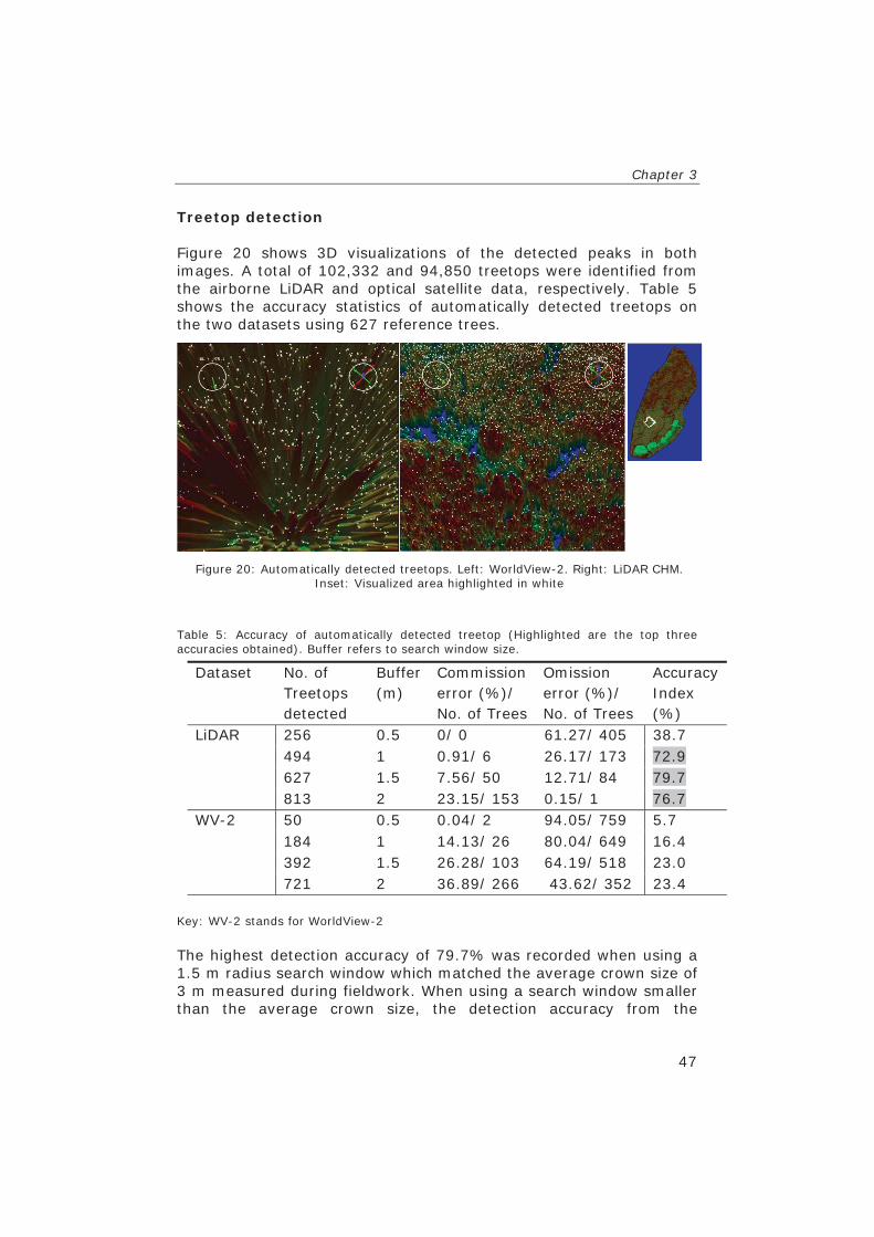
Chapter 3

47

Treetop detection

Figure 20 shows 3D visualizations of the detected peaks in both images. A total of 102,332 and 94,850 treetops were identified from the airborne LiDAR and optical satellite data, respectively. Table 5 shows the accuracy statistics of automatically detected treetops on the two datasets using 627 reference trees.

Table 5: Accuracy of automatically detected treetop (Highlighted are the top three accuracies obtained). Buffer refers to search window size.

Key: WV-2 stands for WorldView-2 The highest detection accuracy of 79.7% was recorded when using a 1.5 m radius search window which matched the average crown size of 3 m measured during fieldwork. When using a search window smaller than the average crown size, the detection accuracy from the

Dataset No. of Treetops detected

Buffer (m)

Commission error (%)/ No. of Trees

Omission error (%)/ No. of Trees

Accuracy Index (%)

LiDAR 256 0.5 0/ 0 61.27/ 405 38.7 494 1 0.91/ 6 26.17/ 173 72.9 627 1.5 7.56/ 50 12.71/ 84 79.7 813 2 23.15/ 153 0.15/ 1 76.7

WV-2 50 0.5 0.04/ 2 94.05/ 759 5.7 184 1 14.13/ 26 80.04/ 649 16.4 392 1.5 26.28/ 103 64.19/ 518 23.0 721 2 36.89/ 266 43.62/ 352 23.4

Figure 20: Automatically detected treetops. Left: WorldView-2. Right: LiDAR CHM. Inset: Visualized area highlighted in white

Results

48

airborne LiDAR data was increasing. The detection accuracy began to decrease when the search window became wider than the average crown size. In the optical satellite data, detection accuracy continued to increase with a wider search window. Individual Crown segmentation

It was hard to visually determine a better segmentation result between LiDAR and WorldView-2 data as shown in Figure 21. However, quantitative accuracy assessment with manually digitized crown data showed that the LiDAR crown delineation was more accurate. Over segmentation error was 11% and 23% in LiDAR and WorldView-2 datasets respectively. Under segmentation error was 32% and 72% in LiDAR and WorldView-2 datasets respectively. Using the closeness index to obtain an overall segmentation accuracy measure, the segmentation from LiDAR data was 86.4% closer to the ideal segmentation in a space defined by the reference polygons. Segmentation from LiDAR had a D-Value score of 0.34. The WorldView-2 segmentation was 69% closer to the reference polygons with a D-Value of 0.76. The LiDAR segmentation output was therefore used to define the individual tree crown boundaries in extraction of the physical and spectral parameters for species identification and classification.

Figure 21: Segmentation results. Left: LiDAR. Right: WorldView-2

Chapter 3

49

3.1.3 Tree physical parameters A linear regression between the image estimated (LiDAR CHM) and ground estimated height showed R2 values of 0.65 and 0.81 before and after removing outliers respectively as shown in Figure 22 (Top). The correlation and R2 values between Image estimated (LiDAR) and ground estimated crown diameter was 0.18 and 0.41 respectively (Figure 22-2Bottom). QQ plots of all the physical parameters (appendix 5) show a normal distribution of the data.

Figure 22: LiDAR derived Tree Height (Top) and Crown diameter (Bottom). Height with outliers (left), Height without outliers (Right), Crown diameter using a circular model

(Left), Crown diameter using an elliptic model (Right)

Results

50

The box plots of within crown standard deviation (SD) and coefficient of variation of intensity show overlap between the species (Figure 23).

Key: PS – Pinus sylvestis PU – Pinus unicinata

3.1.4 Crown spectral parameter Figure 24 shows a species-wise boxplot of within crown maximum Digital Number (DN) values across the WorldView-2 spectral bands. More distinction information based on the mean is available in bands 6, 7 and 8. The spread (distribution) of the DN values, across species, overlaps. The results of other within crown statistics evaluated are presented in Appendix 6.

Figure 23: Intensity Standard Deviation (SD) and Coefficient of Variation (CoV) of the two pine species

Cha

pter

3

51

Key

: PS

_1 –

Pin

us s

ylve

stri

s Ban

d 1

& P

U_1

– P

inus

unc

inat

a Ban

d 1

Figu

re 2

4: M

axim

um W

orld

Vie

w-2

DN

val

ues

per

crow

n an

d be

twee

n sp

ecie

s.

Res

ults

52

Key

: PU

- Pi

nus

unic

inat

a, P

S-

Pinu

s sy

lves

tris

, STD

- Sta

ndar

d de

viat

ion

Figu

re 2

5: W

ithin

cro

wn

stat

istic

s of

Wor

ldVie

w-2

Ban

d 67

8 co

mpo

site

bet

wee

n sp

ecie

s

Cha

pter

3

53

Key

: PU

- Pi

nus

unic

inat

a, P

S-

Pinu

s sy

lves

tris

, STD

- Sta

ndar

d de

viat

ion

Figu

re 2

6: W

ithin

cro

wn

Wor

ldVie

w-2

sat

ellit

e al

bedo

sta

tistic

s be

twee

n sp

ecie

s

Chapter 3

54

Figure 25 shows species-wise boxplots of within crown descriptive statistics of the WorldView-2 spectral Band678 composite. The largest distinction of the species is seen in the within crown maximum DN values of the Band678 and the satellite albedo composites. The boxplot of within crown albedo is shown in Figure 26. A WorldView-2 spectral bands profile of both species was generated based on the mean of the within crown maximum DN values using 807 reference trees (Figure 27). The widest distinction between the species is seen in bands 6, 7 and 8.

3.1.5 Regression modelling The role of Variance Inflation Factor (VIF) in identifying collinearity among predictor variables has already been discussed in chapter 2. VIF values for the individual tree spectral and physical parameters considered in the regression modelling are as shown in Table 6. There was no collinearity between the variables used to predict the species classes.

Figure 27: WorldView-2 spectral profiles of the two tree species

Chapter 3

55

Table 6: Variance Inflation Factors across explanatory variables Variable VIF Height 1.23 Crown Diameter 1.24 Intensity 1.04 Albedo 1.04 The six models evaluated in this study showed similar predictive power ranging from 0.73 to 0.76 of Area Under Curve (AUC) and the map accuracies from 0.44 to 0.54 of Kappa as shown in Figure 28. The best predictive power and map accuracy results were obtained when all the four variables were used as explanatory attributes in both Logistic Regression and CART models (Figure 28). Model coefficients and classification trees have been presented in Appendix 7. The best classification result as obtained from the CART model using both spectral and physical parameters is shown in Figure 29.

Figure 28: Model accuracy results

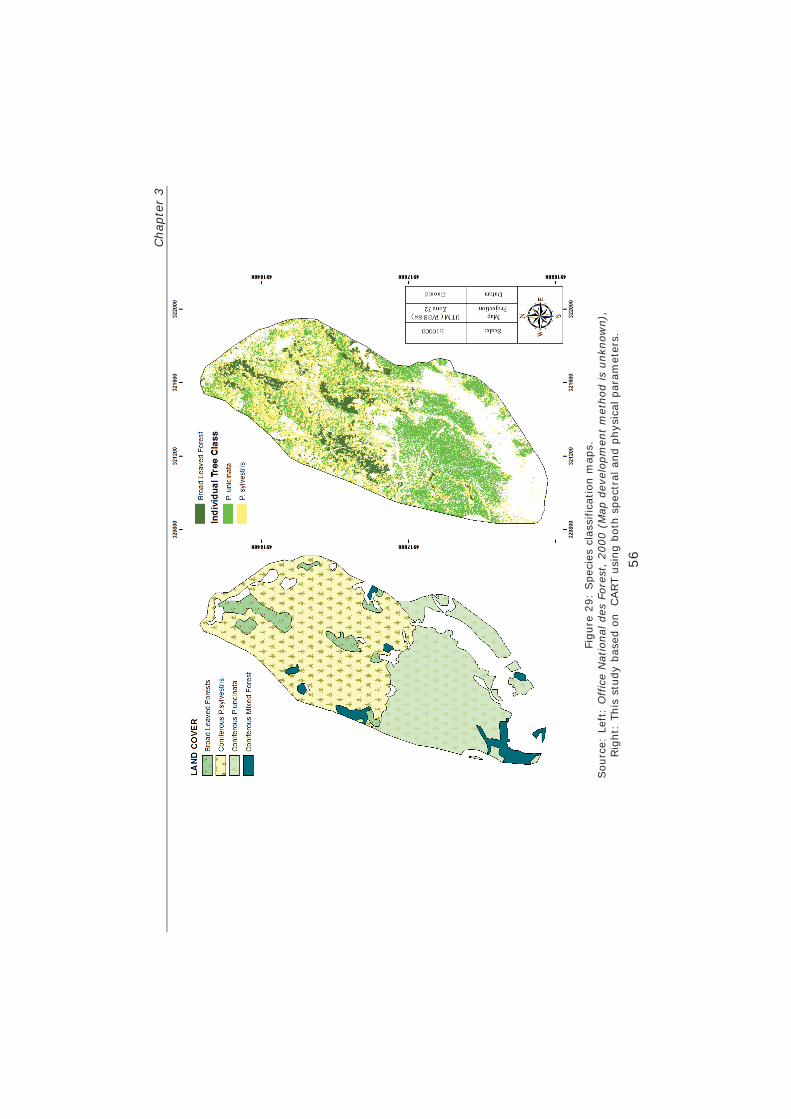
Cha

pter

3

56

Figu

re 2

9: S

peci

es c

lass

ifica

tion

map

s.

Sou

rce:

Lef

t: O

ffic

e N

atio

nal d

es F

ores

t, 2

000

(Map

dev

elop

men

t m

etho

d is

unk

now

n),

Rig

ht:

This

stu

dy b

ased

on

CART

usin

g bo

th s

pect

ral a

nd p

hysi

cal p

aram

eter

s.

57

Chapter 4

4.1 DISCUSSION

4.1.1 Field Methods

This study employed a novel field technique to locate plot centres and identify individual tree locations as has been described in Chapter 2 - field work section. The advantages of this method have been discussed in a section below on individual treetop detection. This method integrated the use of a GPS receiver, the LiDAR CHM, landmarks and ground distance measurements. The technique is well justified given that the accuracy of LiDAR spatial and elevation metrics in forest studies is appreciated (Hodgson & Bresnahan, 2004; Gobakken & Naesset, 2008; Andersen et al., 2009; Kaartinen et al., 2012). LiDAR spatial and elevation errors can still occur especially when associated with system calibration, horizontal displacement, interpolation and the surveyor’s experience (Hodgson & Bresnahan, 2004; Kaartinen et al., 2012). Our CHM showed accurate (Hodgson & Bresnahan, 2004) spatial and elevation information when tested at known locations during reconnaissance and therefore could be used to locate plot centres and individual tree positions in a faster as well as more accurate approach.

However, replication of the aforementioned field technique requires to be done cautiously. This is because our approach does not alleviate the problem of accurately locating treetops during fieldwork at all image scales. Our method is greatly dependent on the image scale in question. At fine image scales, like our 0.15 m LiDAR CHM resolution, it guarantees less than a single crown margin of error. However, its application at larger image scales may introduce errors. In their study, Wang et al. (2004) note that image intensity changes can occur over a wide range of scales. At a fine scale - as in our LiDAR CHM - all branches in a tree crown image are visible thus enabling location of the treetop position near a local ‘geometric peak’. However, at a coarser scale – such as in the WorldView-2 image - a single tree crown may merge with its neighbours, thus introducing errors. This technique will therefore require further investigation specifically regarding the effect of scale and human error in the location of treetops on the CHM and plot centres in the field.

Discussion

58

4.1.2 Forest Condition

The statistics showed that Bois noir forest is growing slowly considering that its documented age is over 100 years. The majority of trees in this forest remain low in DBH (Figure 16). Many tree crowns in the study area are small, overlapping, and with a high crown base height. This structure is indicative of competition for photosynthetic resources. Diameter growth is related to tree support, water absorption and leaf biomass, while the height growth is related to light interception (Sönmez, 2009; Li et al., 2011). The low correlation between DBH and height suggests a trade off in resource allocation which is indicative of either water or temperature stress (Wang et al., 2006). Both stresses appear to be at play in this area as the trees undergo both severe cold during winter and suffer water stress due to shallow soils along the steep slopes. These stresses are compounded by the lack of silvicultural practices like thinning and therefore despite the fact that needle leaved species can escape the harm of winter conductance, excessive branches on the tree stem cause the trees to suffer irreversible loss to water conductance of xylem during winter. Thus more resources are allocated for sap wood growth during the growing season to maintain the necessary water conductance (Wang et al., 2006). However, a few trees of high DBH exist in areas with lower slope and deeper soils, mainly on plateaus and are the outliers seen in Figure 16. On the other hand, the high tree density, could account for low correlations between crown diameter and DBH. While we fitted a linear function, Sönmez (2009) suggests a cubic relationship between crown diameter and DBH for a Pinaceae species (Picea orientalis) which further explains the low correlation values.

4.1.3 Geometric co-registration of datasets

This study achieved a co-registration root mean square error (RMSE) of one pixel (0.5 m) between the LiDAR and WorldView-2 datasets using six ground control points and a LiDAR derived DEM as illustrated in Figure 3. The use of more ground control points could have improved the co-registration accuracy. However, due to variability in the canopy structure, shadow effects (Figure 4) and topographic distortions (Figure 30), addition of tie points resulted in higher RMSE. The steep slopes of varying aspect, sun elevation (48.1) and azimuth (161.7) angles and the average satellite elevation (74.8) and azimuth (55.0) angles explain the shadows on the scene. The ragged landscape explains the geometric distortions. Fuzziness is spread across the image which made precise tying of features in the images impossible. Moreover, unlike man-made structures, natural

Chapter 4

59

landscape features do not often have discrete symmetrical edges (Ben-Arie, 2009) hence introducing uncertainty in positioning of tie points. The use of accurate ground control points (GCP) would alleviate these uncertainties and improve the co-registration result; however this data was not available for this study and can be very time consuming to collect. A faster attempt (i.e. without connection to a local base station) to collect ground control points using a DGPS was made. However, the collected points required post processing to achieve within centimetre accuracy. We were not able to get recordings from a local base station within the time available for this study.

4.1.4 Treetop Identification The spatial profiles generated over the grey scale images (Figures 17) suggested higher commission errors in treetop detection from the satellite imagery than the LiDAR CHM. Our tree detection accuracy assessment results presented in Table 5 confirmed these higher commission errors in WorldView-2. The spectral peaks in the panchromatic image did not necessarily represent topographic peaks (as suggested by Wang et al. (2004)) as did the geometric peaks in the LiDAR data. In some parts of the WorldView-2 satellite imagery, these local peaks represented the colour contrast between the tree crowns and the background an effect brought about by a high signal to noise ratio especially shadows. Figure 31 demonstrates this effect. However, although LiDAR performed better than WorldView-2 in individual tree detection (z-test P=7.9x10-7, =0.05), there are considerable omission and commission errors. There was generally higher omission than commission error recorded in both datasets

Figure 30: Topographic distortions. Left: WorldView-2 Image after geometric correction. Right: WorldView-2 Image before geometric correction.

Discussion

60

(Table 5). These errors can be explained by the effect of a fixed window size based on the mean crown radius. It appears that a fixed window size was not representative of very small as well as very large crowns hence omission and commission errors, respectively. Even though Wulder et al. (2000) show that there is no significant difference between the rate of correct predictions between either the fixed or variable window size of local maximum strategy, they report a reduction in commission error when using variable window sizes. It therefore remains a trade-off between total proportion of trees correctly identified and the level of commission and omission error to be accommodated whereby a larger than optimal window results in higher omission error because it contains multiple tree apexes or a smaller than optimal window size, too many apexes are identified (commission errors) because the small window does not always contain a true tree apex (Pouliot et al., 2002). However, we note that a fixed window size based on mean crown diameter provides a simple and quick alternative to estimate tree positions from high density LiDAR to optimal accuracies even in forest with a complex condition as Bois noir. This study’s tree detection accuracies are hard to compare with other studies given the variation in LiDAR point densities, satellite image resolutions, filtering and detection methods as well as terrain form. As previously mentioned, we employed a simpler and probably less preferred fixed window local maximum filtering approach. Nonetheless, our LiDAR result was good compared to other studies. Persson et al. (2002) had 71% tree detection accuracy employing

Figure 31: Automatically detected treetops from WorldView-2 panchromatic image

Chapter 4

61

variable Gaussian filters and local maximum filtering on a 2 points per m2 dataset at a site supposedly less mountainous. Similarly, Véga and Durrieu (2011) achieved a 73.97% tree detection using multi-level 3x3 Gaussian low pass filtering before employing the local maximum algorithm on a 5 points per m2 dataset and at a site with mountainous terrain. We achieved better accuracy (79.7%) than the mentioned studies. Our ‘good’ treetop detection result from LiDAR data can be partly attributed to precise location of reference trees during fieldwork, a higher point density and a good choice of local maximum filtering window. We were able to accurately locate reference trees in the field a step that enhanced our accuracy assessment. Difficulty associated with identifying tree locations in the field has limited studies in the past to less robust aggregated accuracy assessments (Gougeon, 1995) than individual tree detection accuracy assessments used in this study (Pouliot et al., 2002). Many other studies later in time (Wulder et al., 2000; Pouliot et al., 2002; Wulder et al., 2002; Wulder et al., 2004) have equally recognized this challenge of locating trees in the field as affecting individual tree detection accuracy results. With further investigation of our field method, this challenge of locating trees in the field could be alleviated. On the other hand, higher LiDAR point densities gave this study the upper hand given the reduced generalization of tree crown characteristics in the CHM. It was possible to locate treetops in the grey scale image. Higher height values are visibly brighter than lower values in the image enabling optimal location of treetops. A window size commensurate to the mean tree crown width measured in the field accounted for the challenge of identifying the right kernel in this moving-window procedure hence improving detection accuracies. Treetop detection in the WorldView-2 imagery gave a result similar to other studies despite the high signal to noise ratio, topographic distortions and low resolution in respect to crown sizes. While relating crown radius measured in the field to the proportion of correctly identified trees in 1 m resolution imagery, Wulder et al. (2000) had proportions of trees identified by local maximum filters at 13%, 32% and 51% for three fixed window sizes of 3x3, 5x5 and 7x7 respectively. They attributed the low detection accuracies to generalizations applicable for the object resolution relationship existing between the 1 m spatial resolution image data and the field data under consideration. Bois noir forest is not privy to this as it is characteristic of small crowns (mean crown radius of 3m) and therefore a 0.5m resolution significantly generalizes the crown structure obscuring many peaks (Pouliot et al., 2002). Conversely,

Discussion

62

Wulder et al. (2004) attribute their high proportions of correctly identified trees in IKONOS imagery (80%-92% across ranges of crown radii) to a high sun angle and lack of shadows in the imagery and therefore concluded that IKONOS provides sufficient information on individual tree locations to allow meaningful studies of forest structure. Although WorldView-2 satellite imagery has a finer spatial resolution than IKONOS imagery, its application in a mountainous terrain was not that good. Our individual tree detection result was poor mainly because the scene was greatly affected by off nadir viewing geometric distortions, low resolution in respect to image objects, topographic distortions and a low sun angle leading to shadowing. These factors accounted for a higher signal to noise ratio in the imagery which precluded accurate identification of individual tree locations by their treetop (Figures 30 & 31). Whether both omission and commission error accommodated in this study could be completely eliminated in a synergistic approach using variable window sizes remains a matter that this study could not address given its scope. Similarly, the combined application of LiDAR and WorldView-2 in tree detection was not feasible given the wide range in accuracies between the two datasets. Treetops from both datasets were therefore used independently as seed pixels to grow the individual tree crowns.

4.1.5 Crown segmentation A region growing segmentation method works well if only one seed point in each crown can be detected (Erikson & Olofsson, 2005). We attribute over segmentation and under segmentation errors to commission and omission errors accommodated at the tree detection step, respectively. These errors have been well described by Ke and Quackenbush (2011). As expected, LiDAR derived segments were more accurate than the WorldView-2 when analyzed against 1615 reference individual crown polygons. A segmentation accuracy of 86.4% was achieved from the LiDAR data. Unexpectedly, segmentation accuracy was higher than treetop detection accuracy at 79.7%. This is because segmentation accuracy reported can be misleading due to the potential for accommodated commission and omission errors from the tree detection step to cancel out (Ke & Quackenbush, 2011). The visually distinguishable trees in the image are not always the trees on ground due to overlaps in the canopy. Similarly, some trees may grow in lower canopy strata and are missed in the imagery. This problem of overestimated segmentation accuracy can be tackled in part by using field delineated crowns as reference for accuracy assessment. However, collection of this data

Chapter 4

63

will significantly increase the time required to conduct field work and will still remain inaccurate in the closed canopy. A significantly higher under segmentation error was observed in the WorldView-2 imagery even though the total number of seed pixels identified in both datasets was similar. This finding affirms the significant mislocation of treetops in the WorldView-2 satellite data as illustrated in Figure 31. The low performance of the WorldView-2 satellite imagery in segmentation of individual crowns was mainly due to low resolution in respect to the crown sizes. Individual tree crowns must be visually distinguishable in the image before any thresholding based on colour or shape can be employed successfully. The generalizations coupled with shadows and distortions in the image obscured contrast between the tree crowns and the background which made accurate individual tree crown segmentation infeasible. Crown regions were overgrown leading to higher under segmentation error.

4.1.6 Tree physical parameters

A relatively low goodness of fit (0.65 for height and 0.18 for crown diameter) was achieved when field estimated and LiDAR estimated tree height and crown diameter were compared. This finding was unexpected for height estimates given that studies have showed higher correlations and R2 between tree measurements acquired from LiDAR and those acquired using traditional field methods (Persson et al., 2002; Andersen et al., 2006). However, most studies have compared LiDAR estimated height to field estimated height from laser instruments. In this study, we used a Haga© to estimate tree height in the field which could explain the inconsistence with our findings (Persson et al., 2002; Wing et al., 2004). Moreover, considering that the dominant source of error in LiDAR tree height measurement is due to the difficulty in measuring treetop locations during fieldwork, the existence of pits in the CHM may have led to underestimation of height if a field determined treetop location fell on a pit in the CHM. Ben-Arie et al. (2009) proposed a pit filling algorithm for LiDAR canopy height models to increase their quality. We were not able to employ such a pit filling algorithm in the time available for this study but used mean filters to eliminate pits. This could have introduced errors in estimation. Similarly, the accuracy of LiDAR data in tree height estimation in mountainous terrain also requires to be further investigated. Unlike the high correlation and low root mean square errors recorded in a review by Andersen et al. (2006), Kwak et al. (2007) had a lower goodness of fit (0.74) working in a mountainous area in central South Korea. Whether or

Discussion

64

not there was significant vertical error introduced by our LiDAR data was beyond the scope of this study but cannot be overlooked as having had an effect on the result. On the other hand, the low coefficient of determination between field estimated and LiDAR estimated crown diameter was expected. This is because of the already discussed treetop detection and segmentation errors, the well-known errors in field estimation and errors from the assumed elliptic shape of tree crowns. We opted to restrict our analysis to three physical parameters because a regression modelling approach was to be used for species classification. Predictor variables for regression modelling require to have low collinearity and other parameters like crown volume and crown projection area that could be computed from LiDAR metrics were derivatives of crown diameter and tree height. Other parameters like crown tilt, crown orientation, crown density, local crown gaps percentage could not be used because of issues related to model transferability. Crown intensity was introduced experimentally to evaluate whether it would have a significant contribution to species classification. However, Figure 23 shows that the intensity values between the species were closely related.

4.1.7 Crown spectral parameter

Various statistical summaries of individual crown from WorldView-2 satellite data were evaluated and a spectral signature (Figure 27) was extracted. The signature indicated spectral distinction between the two closely related tree species. Higher distinction information was possible in bands 6, 7 and 8. The maximum within crown values gave better distinction than other statistics evaluated (Figures 25 & 26 and appendix 6). This can be attributed to the high signal to noise ratio in the satellite image. The extraction of maximum spectral values appears to have distinguished the crown reflectance from background reflectance in the image and ‘purified’ the species spectral signal. However, this is a new technique that appears conceptually feasible but requires further investigation on a wider range of species.

4.1.8 Tree species identification

By mapping the extracted within crown spectral and physical parameters to treetops, the integration of LiDAR and satellite data for species classification was possible through regression modelling. The predictive power of the models was similar (Figure 28) despite the classifiers using completely different approaches. This is a promising

Chapter 4

65

finding as it affirms that spectral and physical characteristics are robust predictors of species classes. The low predictive power of the models can be qualified by the quality of the input data as previously discussed. More accurate estimates of predictor variables could result in higher predictive power by the models.

Classifications accuracy has been evaluated using the Kappa coefficient. Kappa was similar across models as well as predictor variables. In this case, the Kappa value is highly dependent on the threshold assigned to distinguish the species. A 50% threshold was used in this study whereby the predicted values below 0.5 were assigned to Pinus uncinata and above 0.5 to Pinus sylvestris. However, using the same dataset to drive the model, variant thresholds would result into significantly different Kappa results. For example, the alternative threshold would be to use field estimated species abundance or dominance considering that these measures indicate the rate of species occurrence. A threshold based on the rate of occurrence could improve model specificity and sensitivity. This was not investigated in this study but can be considered an option for further research.

The combination of LiDAR and spectral attributes showed a marginal increase in species distinction. Appendix 7 shows the model coefficients. The P-values show that all the variables had a significant contribution in the distinction of species. This was expected given the lack of collinearity among predictor variables. Spectral data had the most significant influence in the runs where both datasets were combined and for both model types (Appendix 7). This finding was unexpected, considering the signal to noise ratio in the WorldView-2 spectral data. However, this finding further supports the idea of ‘spectral purification’ using simple statistical summaries and can be considered in future work. We have tested our species classification approach with two basic models using easy to compute statistical variables. The time consuming task was variable extraction, but models run quickly for over 100,000 individual tree data. This approach can be further studied as we have proposed in the recommendations.

Discussion

66

67

Chapter 5

5.1 CONCLUSION AND RECOMMENDATIONS

5.1.1 Conclusion We have examined three individual crown segmentation and species identification and classification schemes i.e. segmentation and species identification and classification based on LiDAR layers, spectral layers and a combination of the two datasets. Using segmentation goodness measures proposed by Clinton et al. (2010) to assess individual crown segmentation quality and Kappa statistics to assess the accuracy of species identification and classification, we have found out that LiDAR derived individual crown segments were superior (Segmentation goodness = 86.4% closer to the reference polygons) to the WorldView-2 optical satellite individual crown segments (Segmentation goodness = 69% closer to the reference polygons). We also conclude that the integration of the datasets for individual tree species identification and classification using a regression modelling approach provided increased interpretation capabilities and an opportunity for more reliable results. The best classification result (Kappa=54%) was obtained from the Classification and Regression Trees model using both the crown spectral parameter derived from WorldView-2 satellite data and tree physical parameters derived from LiDAR data as predictor variables. Although the integration of LiDAR and WorldView-2 was not possible to be achieved for this study, it is still conceptually feasible. The application of WorldView-2 imagery at our mountainous study site was not that good. The poor performance of the WorldView-2 optical satellite imagery owed to the distortions and scale issues as has been discussed. These inconsistences in the WorldView-2 optical satellite data hindered the integration of the two datasets for individual crown segmentation. Both LiDAR and WorldView-2 optical satellite imagery had a similar contribution to individual tree species identification and classification. There was no significant difference in Kappa statistics of individual tree species classification maps obtained from either LiDAR derived tree physical parameters or the WorldView-2 optical satellite spectral parameter used in isolation. However we learn that the crown

Conclusions and Recommendations

68

spectral parameter was marginally stronger than the tree physical parameters in differentiation of the two tree species, a step we have attributed to ‘spectral purification’. Several novel techniques have proposed and experimented with and new findings discovered by this study that will require further investigation as highlighted in the recommendations.

5.1.2 Recommendations

1. This study was conceived on a conceptually firm ground as discussed in the background. However, various bottlenecks related to the quality of the WorldView-2 optical satellite imagery were met along the way. Many of these bottlenecks culminated from the effect of terrain and image sun elevation angle but not all WorldView-2 imagery have these negative effects. We therefore recommend a similar study in a flat terrain and an optimal sun elevation angle so as to eliminate the bias brought about by the high signal to noise ratio in the WorldView-2 optical satellite imagery used in this study. A good alternative will be to test our methods with the 15 cm ortho-photo collected with the LiDAR dataset.

2. Further investigation of the field method used by this study to

identify locations of individual treetops and plot centres in the field will be required so as to evaluate the effect of human error and image scale on the accuracy of the data collected.

3. We proffer further investigation on the effect of variable window sizes in the local maximum filtering strategy to locate treetops on both the LiDAR CHM and the panchromatic WorldView-2 optical satellite imagery. This strategy may further reduce commission and omission errors in tree detection.

4. The effect of a pit filling algorithm on improving the quality of the CHM for treetop detection and individual crown segmentation requires to be further studied. This study tried mean filters and found out that mean filters appear to introduce vertical error in height estimations and that they only reduce than remove the pits completely.

5. There is need to investigate the accuracy of LiDAR height metrics versus field based estimates in mountainous terrain. Our experience using analogue instruments to estimate tree height in the field provides premise to raise suspicion towards

Chapter 5

69

inaccuracies in field based height estimates than LiDAR derived height metrics. However, this requires further investigation.

6. The ability to overcome the optical imagery high signal to noise ratios in a ‘spectral purification’ step using maximum within crown spectral values requires to be further investigated. This will be best done comparing among various tree species. The potential of this method to distinguish closely related species using hyper-spectral data appears promising.

7. This study suffered effects of error propagation in the estimation of both crown spectral and tree physical parameters. Further study can be directed towards understanding the magnitude of error propagated and its effect on the quality of data extracted from both datasets (LiDAR and WorldView-2 optical satellite imagery). Similarly, regression modelling approaches with stronger predictive power like the boosted regression trees can be investigated for better predictive power and Kappa statistics in our species identification approach.

Conclusions and Recommendations

70

71

References Andersen, H.E., Reutebuch, S.E. & McGaughey, R.J. (2006) A

rigorous assessment of tree height measurements obtained using airborne lidar and convetional field methods. Canadian Journal of Remote Sensing, 32, 355-366.

Andersen, H.E., Clarkin, T., Winterberger, K. & Strunk, J. (2009) An acuracy assessment of positions obtained using survey- and recreational-grade Global Positioning System Receivers across a range of forest conditions within the Tanana valley of interior Alaska. West. J. Appl. For., 24, 128-136.

Ben-Arie, J.R., Hay, G.J., Powers, R.P., Castilla, G. & St-Onge, B. (2009) Development of a pit filling algorithm for LiDAR canopy height models. Computers & Geosciences, 35, 1940-1949.

Bi, H., Fox, J.C., Li, Y., Lei, Y. & Pang, Y. (2012) Evaluation of nonlinear equations for predicting diameter from tree height. Canadian Journal of Forest Research, 42, 789-806.

Brandtberg, T. & Walter, F. (1998) Automated delineation of individual tree crowns in high spatial resolution aerial images by multiple-scale analysis. Machine Vision and Applications, 11, 64-73.

Brandtberg, T., Warner, T.A., Landenberger, R.E. & McGraw, J. (2003) Detection and analysis of individual leaf-off tree crowns in small footprint, high sampling density lidar data from the eastern deciduous forest in North America. Remote Sensing of Environment, 85, 290-303.

Breiman, L., Friedman, F., Olshen, R. & Stone, C. (1984) Classification and regression trees Wadsworth, Pacific Grove, CA, US.

Buma, J. (2000) Finding the most suitable slope stability model for the assessment of the impact of climate change on a landslide in southeast France. Earth Surface Processes and Landforms, 25, 565-582.

Carleer, A. & Wolff, E. (2004) Exploitation of Very High Resolution Satellite Data for Tree Species Identification. Photogrammetric Engineering and Remote Sensing, 70, 135-140.

Chen, Q., Baldocchi, D., Gong, P. & Kelly, M. (2006) Isolating individual trees in a savanna woodland using small footprint lidar data. Photogrammetric Engineering and Remote Sensing, 72, 923-932.

Chen, Q., Vaglio Laurin, G., Battles, J.J. & Saah, D. (2012) Integration of airborne lidar and vegetation types derived from aerial photography for mapping aboveground live biomass. Remote Sensing of Environment, 121, 108-117.

References

72

Cho, M.A., Naidoo, L., Mathieu, R. & Asner, G.P. (2011) Mapping savanna tree species using Carnegie Airborne Observatory hyperspectral data resampled to WorldView-2 multispectral configuration.

Clinton, N., Holt, A., Scarborough, J., Yan, L. & Gong, P. (2010) Accuracy Assessment Measures for Object-based Image Segmentation Goodness. Photogrammetric Engineering and Remote Sensing, 76, 289-299.

Dalponte, M., Bruzzone, L. & Gianelle, D. (2011) A system for the estimation of single-tree stem diameter and volume using multireturn LIDAR data. Ieee Transactions on Geoscience and Remote Sensing, 49, 2479-2490.

Deng, F., Li, S. & Su, G. (2007) A methodology for fusion LIDAR and digital images. 67952C-67952C.

Digital-Globe (2010) Radiometric use of WorldView-2 Imagery. In: Technical Note pp. 1-17. Digital-Globe

Digital-Globe (2013) WorldView-2. Available at: http://www.digitalglobe.com/about-us/content-collection#satellites&worldview-2 (accessed 21/01/2013)

Dorren, L.K.A., Maier, B. & Seijmonsbergen, A.C. (2003) Improved Landsat-based forest mapping in steep mountainous terrain using object-based classification. Forest Ecology and Management, 183, 31-46.

Erikson, M. (2004) Species classification of individually segmented tree crowns in high-resolution aerial images using radiometric and morphologic image measures. Remote Sensing of Environment, 91, 469-477.

Erikson, M. & Olofsson, K. (2005) Comparison of three individual tree crown detection methods. Machine Vision and Applications, 16, 258-265.

ESRI (2011) LIDAR analysis in ArcGIS 10 for forestry applications. In. ESRI New York

FAO (1998) A manual for the planning, design and construction of forest roads in steep terrain In. FAO Forestry Department

FAO (2012) State of the World's Forests 2012. Fauvart, N., Ali, A.A., Terral, J.-F., Roiron, P., Blarquez, O. &

Carcaillet, C. (2012) Holocene upper tree-limits of Pinus section sylvestris in the Western Alps as evidenced from travertine archives. Review of Palaeobotany and Palynology, 169, 96-102.

Flageollet, J.C., Malet, J.P. & Maquaire, O. (2000) The 3D structure of the Super-Sauze earthflow: A first stage towards modelling its behaviour. Physics and Chemistry of the Earth Part B-Hydrology Oceans and Atmosphere, 25, 785-791.

References

73

Flageollet, J.C., Maquaire, O., Martin, B. & Weber, D. (1999) Landslides and climatic conditions in the Barcelonnette and Vars basins (Southern French Alps, France). Geomorphology, 30, 65-78.

Florinsky, I.V. (1998) Combined analysis of digital terrain models and remotely sensed data in landscape investigations. Progress in Physical Geography, 22, 33-60.

Franklin, S.E., Maudie, A.J. & Lavigne, M.B. (2001) Using Spatial Co-Occurrence Texture to Increase Forest Structure and Species Composition Classification Accuracy Photogrammetric Engineering and Remote Sensing, 67, 849-855.

Garcia, M., Riano, D., Chuvieco, E. & Danson, F.M. (2010) Estimating biomass carbon stocks for a Mediterranean forest in central spain using LiDAR height and intensity data. Remote Sensing of Environment, 114, 816-830.

Gebreslasie, M.T., Ahmed, F., van Aardt, J.A.N. & Blakeway, F. (2011) Individual tree detection based on variable and fixed window size local maxima filtering applied to IKONOS imagery for even-aged Eucalyptus plantation forests. International Journal of Remote Sensing, 32, 4141-4154.

Gong, P., Pu, R. & Yu, B. (1997) Conifer species recognition: An exploratory analysis of in situ hyperspectral data. RemoteSensing of Environment, 62, 189-200.

Gong, P., Sheng, Y. & Biging, G. (2002) 3D Model-Based Tree Measurement from High-Resolution Aerial Imagery. Photogrammetric Engineering and Remote Sensing, 68, 1203-1212.

Gougeon, F. (1995) Crown-Following Approach to the Automatic Delineation of Individual Tree Crowns in High Spatial Resolution Aerial Images. Canadian Journal of Forest Research, 21, 274-284.

Gougeon, F.A. & Leckie, D.G. (2006) The individual tree crown approach applied to Ikonos images of a coniferous plantation area. Photogrammetric Engineering and Remote Sensing, 72, 1287-1297.

Gurram, P., Hu, S. & Chan, A. (2013) Uniform grid upsampling of 3D lidar point cloud data. SPIE 8650, Three-Dimensional Image Processing (3DIP) and Applications (ed by, p. 86200B.

Hauser-Davis, R., Oliveira, T., Silveira, A., Protázio, J. & Ziolli, R. (2012) Logistic regression and fuzzy logic as a classification method for feral fish sampling sites. Environmental and Ecological Statistics, 19, 473-483.

Hay, G.J., Castilla, G., Wulder, M.A. & Ruiz, J.R. (2005) An automated object-based approach for the multiscale image

References

74

segmentation of forest scenes. International Journal of Applied Earth Observation and Geoinformation, 7, 339-359.

Heinzel, J. & Koch, B. (2012) Investigating multiple data sources for tree species classification in temperate forest and use for single tree delineation. International Journal of Applied Earth Observation and Geoinformation, 18, 101-110.

Hilty, J. (2012) Illinois Wildflowers. Available at: http://www.illinoiswildflowers.info/trees/plants/scots_pine.html (accessed 27/3/2013 2013).

Holmgren, J., Persson, Å. & Söderman, U. (2008) Species identification of individual trees by combining high resolution LiDAR data with multi spectral images. International Journal of Remote Sensing, 29, 1537-1552.

Hyyppa, J., Kelle, O., Lehikoinen, M. & Inkinen, M. (2001) A segmentation-based method to retrieve stem volume estimates from 3-D tree height models produced by laser scanners. Geoscience and Remote Sensing, IEEE Transactions on, 39, 969-975.

Jensen, J.R. (2007) Remote sensing of the environment. An earth resource perspective. Pearson Education Inc., Upper Saddle River, USA.

Jing, L.H., Hu, B.X., Noland, T. & Li, J.L. (2012) An individual tree crown delineation method based on multi-scale segmentation of imagery. ISPRS Journal of Photogrammetry and Remote Sensing, 70, 88-98.

Kaartinen, H., Hyyppä, J., Yu, X., Vastaranta, M., Hyyppä, H., Kukko, A., Holopainen, M., Heipke, C., Hirschmugl, M., Morsdorf, F., Næsset, E., Pitkänen, J., Popescu, S., Solberg, S., Wolf, B.M. & Wu, J.-C. (2012) An International Comparison of Individual Tree Detection and Extraction Using Airborne Laser Scanning. Remote Sensing, 4, 950-974.

Kato, A., Moskal, L.M., Schiess, P., Swanson, M.E., Calhoun, D. & Stuetzle, W. (2009) Capturing tree crown formation through implicit surface reconstruction using airborne lidar data. Remote Sensing of Environment, 113, 1148-1162.

Ke, Y. & Quackenbush, L.J. (2011) A comparison of three methods for automatic tree crown detection and delineation from high spatial resolution imagery. International Journal of Remote Sensing, 32, 3625-3647.

Ke, Y., Quackenbush, L.J. & Im, J. (2010) Synergistic use of QuickBird multispectral imagery and LIDAR data for object-based forest species classification. Remote Sensing of Environment, 114, 1141-1154.

Kim, McGaughey, R.J., Andersen, H.E. & Schreuder, G. (2009a) Tree species differentiation using intensity data derived from leaf-

References

75

on and leaf-off airborne laser scanner data. Remote Sensing of Environment, 113, 1575-1586.

Kim, M., Madden, M. & Warner, T.A. (2009b) Forest Type Mapping using Object-specific Texture Measures from Multispectral Ikonos Imagery: Segmentation Quality and Image Classification Issues. Photogrammetric Engineering and Remote Sensing, 75, 819-829.

Kim, S.-R., Kwak, D.-A., oLee, W.-K., Son, Y., Bae, S.-W., Kim, C. & Yoo, S. (2010) Estimation of carbon storage based on individual tree detection in Pinus densiflora stands using a fusion of aerial photography and LiDAR data. Science China Life Sciences, 53, 885-897.

Koch, B. (2010) Status and future of laser scanning, synthetic aperture radar and hyperspectral remote sensing data for forest biomass assessment. ISPRS Journal of Photogrammetry and Remote Sensing, 65, 581-590.

Koch, B., Heyder, U. & Weinacker, H. (2006) Detection of Individual Tree Crowns in Airborne Lidar Data. Photogrammetric Engineering and Remote Sensing, 72, 357-363.

Kosaka, N., Akiyama, T., Bien, T. & Kojima, T. (2005) Forest type classification using data fusion of multispectral and panchromatic high-resolution satellite imageries. Geoscienceand Remote Sensing Symposium, 2005. IGARSS '05. Proceedings. 2005 IEEE International (ed by, pp. 2980-2983.

Kumar, V. (2012) Forest inventory parameters and carbon mapping from airborne LIDAR. MSc Thesis University of Twente Faculty of Geo-Information and Earth Observation (ITC), Enschede.

Kwak, D.-A., Lee, W.-K., Lee, J.-H., Biging, G. & Gong, P. (2007) Detection of individual trees and estimation of tree height using LiDAR data. Journal of Forest Research, 12, 425-434.

Leckie, D., Gougeon, F., Hill, D., Quinn, R., Armstrong, L. & Shreenan, R. (2003) Combined high-density lidar and multispectral imagery for individual tree crown analysis. Canadian Journal of Remote Sensing, 29, 633-649.

Li, L., Wang, X., Zerbe, S., Zhang, L. & Fang, J. (2011) Altitudinal patterns of stand structure and herb layer diversity of Piceasckrenkiana forests in the central Tianshan Mountains, Northwest China. . Journal of Arid Land, 3, 254-250.

Lim, K., Treitz, P., Wulder, M., St-Onge, B. & Flood, M. (2003) LiDAR remote sensing of forest structure. Progress in Physical Geography, 27, 88-106.

Liu, J.G. (2000) Smoothing Filter-based Intensity Modulation: a spectral preserve image fusion technique for improving spatial details. International Journal of Remote Sensing, 21, 3461-3472.

References

76

Liu, Y., Li, M., Mao, L., Xu, F. & Huang, S. (2006) Review of remotely sensed imagery classification patterns based on object-oriented image analysis. Chinese Geographical Science, 16, 282-288.

Lui, W. & Yamazaki, F. (2012) Object-Based Shadow Extraction and Correction of High-Resolution Optical Satellite Images. IEEEJournal of Selected Topics in Applied Earth Observation and Remote sensing, 5, 1296-1302.

Malet, J.P., Remaitre, A., Maquaire, O., Durand, Y., Etchevers, P., Guyomarc'h, G., Deque, M. & van Beek, L.P.H. (2008) Assessing the influence of climate change on the activity of landslides in the Ubaye Valley Journees Alea Gravitaire (JAG), 8

Maquaire, O., Malet, J.P., Remaitre, A., Locat, J., Klotz, S. & Guillon, J. (2003) Instability conditions of marly hillslopes: towards landsliding or gullying? The case of the Barcelonnette Basin, South East France. Engineering Geology, 70, 109-130.

Martinez Morales, R., Miura, T. & Idol, T. (2008) An assessment of Hawaiian dry forest condition with fine resolution remote sensing. Forest Ecology and Management, 255, 2524-2532.

McCullagh, M. (1988) Terrain and surface modelling systems: theory and practice. The photogrammetric record 12, 747-779.

Meyer, F. & Beucher, S. (1990) Morphological Segmentation. Visual Communication and Image Representation, 1, 21-46.

Möller, M., Lymburner, L. & Volk, M. (2007) The comparison index: A tool for assessing the accuracy of image segmentation. International Journal of Applied Earth Observation and Geoinformation, 9, 311-321.

Munoz, J. & Felicisimo, A.M. (2004) Comparison of statistical methods commonly used in predictive modelling. Journal of Vegetation Science, 15, 285-292.

Mutanga, O. & Skidmore, A.K. (2004) Narrow band vegetation indices overcome the saturation problem in biomass estimation. International Journal of Remote Sensing, 25, 3999-4014.

Nabuurs, G.J.O.M., K. Andrasko, P. Benitez-Ponce, R. Boer, M. Dutschke, E. Elsiddig, J. Ford-Robertson, P. Frumhoff, T. Karjalainen, O. Krankina, W.A. Kurz, M. Matsumoto, W. Oyhantcabal, N.H. Ravindranath, M.J. Sanz Sanchez, X. Zhang (2007) Forestry in Climate Change: Mitigation. In: Fourth Assessment Report of the Intergovernmental Panel on Climate Change (ed. O.R.D. B. Metz, P.R. Bosch, R. Dave, L.A. Meyer). Cambridge University Press, Cambridge, United Kingdom and New York, NY, USA.

Ørka, H.O., Næsset, E. & Bollandsås, O.M. (2009) Classifying species of individual trees by intensity and structure features derived

References

77

from airborne laser scanner data Remote Sensing of Environment, 113, 1163-1174.

Padwick, C., Deskevich, M., Pacifici, F. & Smallwood, S. (2010) WorldView-2 Pan-Sharpening. In: ASPRS 2010 Annual Conference, San Diego, California

Palace, M., Keller, M., Asner, G.P., Hagen, S. & Braswell, B. (2008) Amazon Forest Structure from IKONOS Satellite Data and the Automated Characterization of Forest Canopy Properties. Biotropica, 40, 141-150.

Persson, A., Holmgren, J. & Soderman, U. (2002) Detecting and measuring individual trees using an airborne laser scanner. Photogrammetric Engineering and Remote Sensing, 68, 925-932.

Pitt, D.G., Wagner, R.G., Hall, R.J., King, D.J., Leckie, D.G. & Runesson, U. (1997) Use of remote sensing for forest vegetation management: A problem analysis. ForestryChronicle, 73, 459-477.

Pohl, C. & Van Genderen, J.L. (1998) Review article Multisensor image fusion in remote sensing: Concepts, methods and applications. International Journal of Remote Sensing, 19, 823-854.

Pollock, R. (1996) The automatic recognition of individual trees in aerial images of forests based on synthetic tree crown image model. Doctoral Dissertation,

Popescu, S.C., Wynne, R. H., Scrivani, J. A. (2004) Fusion of small-footprint lidar and multispectral data to etimate plot-level volume and biomass in deciduous and pine forests in Virginia, USA. Forest Science 551-565.

Pouliot, D.A., King, D.J., Bell, F.W. & Pitt, D.G. (2002) Automated tree crown detection and delineation in high-resolution digital camera imagery of coniferous forest regeneration. RemoteSensing of Environment, 82, 322-334.

Puttonen, E., Suomalainen, J., Hakala, T., Räikkönen, E., Kaartinen, H., Kaasalainen, S. & Litkey, P. (2010) Tree species classification from fused active hyperspectral reflectance and LIDAR measurements. Forest Ecology and Management, 260, 1843-1852.

Razak, K.A., Straatsma, M.W., van Westen, C.J., Malet, J.P. & de Jong, S.M. (2011) Airborne laser scanning of forested landslides characterization: Terrain model quality and visualization. Geomorphology, 126, 186-200.

Remaitre, A., Malet, J.P. & Maquaire, O. (2011) Geomorphology and kinematics of debris flows with high entrainment rates: A case study in the South French Alps. Comptes Rendus Geoscience, 343, 777-794.

References

78

Saez, J.L., Corona, C., Stoffel, M. & Berger, F. (2013) Climate change increases frequency of shallow spring landslides in the French Alps. Geology, In press

Saez, J.L., Corona, C., Stoffel, M., Astrade, L., Berger, F. & Malet, J.P. (2012) Dendrogeomorphic reconstruction of past landslide reactivation with seasonal precision: the Bois Noir landslide, southeast French Alps. Landslides, 9, 189-203.

Shreuder, G., McGaughey, R.J. & Andersen, H.E. (2008) Individual tree species identification using LIDAR intensity data. ASPRS Annual Conference (ed by. Portland, Oregon.

Song, C.H., Dickinson, M.B., Su, L.H., Zhang, S. & Yaussey, D. (2010) Estimating average tree crown size using spatial information from Ikonos and QuickBird images: Across-sensor and across-site comparisons. Remote Sensing of Environment, 114, 1099-1107.

Song, J.H., Han, S.H., Yu, K. & Kim, Y.L. (2002) Assessing the possibility of land-cover classification using LIDAR intensity data. In: “Photogrammetric Computer Vision” (ed. I.C. Iii), Gerz.

Sönmez, T. (2009) Diameter at breast height-crown diameter prediction models of Picea orientalis. African Journal of Agricultural Research, 4, 215-219.

Strahler, A.H. (1986) On the Nature of Models in Remote Sensing Remote Sensing of Environment, 20, 121-139.

Straub, C., Dees, M., Weinacker, H. & Koch, B. (2009) Using Airborne Laser Scanner Data and CIR Orthophotos to Estimate the Stem Volume of Forest Stands. Photogrammetrie - Fernerkundung - Geoinformation, 2009, 277-287.

Sugumaran, R. & Voss, M. (2007) Object-Oriented Classification of LIDAR-Fused Hyperspectral Imagery for Tree Species Identification in an Urban Environment. Urban Remote Sensing Joint Event, pp.1-6.

Suratno, A., Seielstad, C. & Queen, L. (2009a) Tree species identification in mixed coniferous forest using airborne laser scanning. ISPRS Journal of Photogrammetry and Remote Sensing, 64, 683-693.

Suratno, A., Seielstad, C. & Queen, L. (2009b) Tree species identification in mixed coniferous forest using airborne laser scanning. ISPRS Journal of Photogrammetry and Remote Sensing, 64, 683-693.

Swatantran, A., Dubayah, R., Roberts, D., Hofton, M. & Blair, J.B. (2011) Mapping biomass and stress in the Sierra Nevada using lidar and hyperspectral data fusion. Remote Sensing of Environment, 115, 2917-2930.

References

79

Thiery, Y., Malet, J.P., Sterlacchini, S., Puissant, A. & Maquaire, O. (2007) Landslide susceptibility assessment by bivariate methods at large scales: Application to a complex mountainous environment. Geomorphology, 92, 38-59.

Thomas, N., Hendrix, C. & Congalton, R.G. (2003) A comparison of Urban Mapping Methods Using High Resolution Digital Imagery Photogrammetric Engineering and Remote Sensing, 69, 963-972.

Tomppo, E., Haakana, M., Katila, M., Peräsaari, J. (2009) Multi-source national forest inventory – Methods and applications. Ann. For. Sci., 66, 47.

Trimble (2011) eCognition Version 8.7 User guide UNEP (2000) The Montreal Protocol on substances that deplete the

ozone layer In. UNEP, Nairobi, Kenya. USGS (2013) Airborne Mapping: mapping methods using airborne

sensors Available at: http://coastal.er.usgs.gov/capabilities/airborne/index.html (accessed 21/01/2013 2013).

Valbuena, R., Mauro, F., Arjonilla, F.J. & Manzanera, J.A. (2011) Comparing airborne laser scanning-imagery fusion methods based on geometric accuracy in forested areas. RemoteSensing of Environment, 115, 1942-1954.

Véga, C. & Durrieu, S. (2011) Multi-level filtering segmentation to measure individual tree parameters based on Lidar data: Application to a mountainous forest with heterogeneous stands. International Journal of Applied Earth Observation and Geoinformation, 13, 646-656.

Wang, L., Gong, P. & Biging, G.S. (2004) Individual tree-crown delineation and treetop detection in high resolution aerial imagery. Photogrammetric Engineering and Remote Sensing, 70, 351-357.

Wang, X., Fang, J., Tang, Z. & Zhu, B. (2006) Climatic control of primary forest structure and DBH-height allometry in Northeast China. Forest Ecology and Management, 234, 264-274.

Wing, M.G., Solmie, D. & Kellogg, L. (2004) Comparing digital range finders for forestry applications. Journal of Forestry, 102, 16-20.

Wulder, Niemann, K.O. & Goodenough, D.G. (2000) Local maximum filtering for the extraction of tree locations and basal area from high spatial resolution imagery. Remote Sensing of Environment, 73, 103-114.

Wulder, M., Niemann, K.O. & Goodenough, D.G. (2002) Error reduction methods for local maximum filtering of high spatial

References

80

resolution imagery for locating trees. Canadian Journal of Remote Sensing, 28, 621-628.

Wulder, M., White, J.C., Niemann, K.O. & Nelson, T. (2004) Comparison of airborne and satelitte high spatial resolution data for identification of individual trees with local maxima filtering International Journal of Remote Sensing, 25, 2225-2232.

Yu, Gong, P., Clinton, N., Biging, G., Kelly, M. & Schirokauer, D. (2006) Object-based detailed vegetation classification with airborne high spatial resolution remote sensing imagery. Photogrammetric Engineering and Remote Sensing, 72, 799-811.

App

endi

ces

81

Ap

pen

dic

es

App

endi

x 1:

Reg

ion

grow

ing

para

met

er s

et

App

endi

ces

82 Reg

ion

grow

ing

para

met

er s

et c

ontin

ued

Appendices

83

Appendix 2: Species classification procedure as implemented in R© ## Set Working Directory setwd("C:\\School\\GEM\\MScProject\\Rawdata_RS\\LiDAR Surfaces\\pre_processingLiDAR\\CHM_0.15") a<-read.csv("Training.csv",header=TRUE, sep=",") b<-read.csv("FinalPeaks_AllData_new.csv",header=TRUE, sep=",") c<-read.csv("Validation.csv",header=TRUE, sep=",") library(ROCR) ##Data exploration ## Testing normality of the variables par(mfrow=c(2,2)) qqnorm(b$CHM_Height) qqnorm(b$eHeight) qqnorm(b$Crown_D) qqnorm(b$Crown_D_E) qqnorm(b$IntSD) qqnorm(b$IntCoV) qqnorm(b$S_Albedo) qqnorm(b$Band687) ##Box plots boxplot (a$CHM_Height,a$eHeight,a$Crown_D,a$Crown_D_E, names=c('CHM Height','Ecog Height','Crown Diameter', 'Crown Diameter ellipse'), yaxis=F, ylab='Meters') boxplot (a$IntSD,xlab=('SD'), ylab='Units') boxplot (a$IntCoV,xlab=('CoV'), ylab='Units') boxplot (a$S_Albedo,xlab=('Maximum Satellite Albedo'), ylab='Digital Numbers') boxplot (a$Band687,xlab=('Maximum 678 Composite'), ylab='Digital Numbers') ##Variable colinearity analysis ##Correlation between variables Numeric<-data.frame(a$CHM_Height,a$eHeight,a$Crown_D,a$Crown_D_E, a$IntSD, a$IntCoV,a$S_Albedo,a$Band687) cor(Numeric) ##Compute VIF for each variable model.CHM_Height <-lm(CHM_Height~Crown_D_E+ IntCoV+S_Albedo+Band687, data=b) r2.CHM_Height<-summary(model.CHM_Height)$r.squared VIF.CHM_Height<-1/(1-r2.CHM_Height) model.Crown_D_E <-lm(Crown_D_E~CHM_Height+IntCoV+S_Albedo+Band687, data=b) r2.Crown_D_E<-summary(model.Crown_D_E)$r.squared VIF.Crown_D_E<-1/(1-r2.Crown_D_E) model.IntCoV <-lm(IntCoV~CHM_Height+Crown_D_E+S_Albedo+Band687, data=b) r2.IntCoV<-summary(model.IntCoV)$r.squared VIF.IntCoV<-1/(1-r2.IntCoV) model.S_Albedo <-lm(S_Albedo~CHM_Height+Crown_D_E+IntCoV+Band687, data=b) r2.S_Albedo<-summary(model.S_Albedo)$r.squared VIF.S_Albedo<-1/(1-r2.S_Albedo)

Appendices

84

model.Band687<- lm(Band687~CHM_Height+Crown_D_E+IntCoV+S_Albedo, data=b) r2.Band687<-summary(model.Band687)$r.squared VIF.Band687<-1/(1-r2.Band687) ##Without Band 678 model.CHM_Height <-lm(CHM_Height~Crown_D_E+ IntCoV+S_Albedo, data=b) r2.CHM_Height<-summary(model.CHM_Height)$r.squared VIF.CHM_Height<-1/(1-r2.CHM_Height) model.Crown_D_E <-lm(Crown_D_E~CHM_Height+IntCoV+S_Albedo, data=b) r2.Crown_D_E<-summary(model.Crown_D_E)$r.squared VIF.Crown_D_E<-1/(1-r2.Crown_D_E) model.IntCoV <-lm(IntCoV~CHM_Height+Crown_D_E+S_Albedo, data=b) r2.IntCoV<-summary(model.IntCoV)$r.squared VIF.IntCoV<-1/(1-r2.IntCoV) model.S_Albedo <-lm(S_Albedo~CHM_Height+Crown_D_E+IntCoV, data=b) r2.S_Albedo<-summary(model.S_Albedo)$r.squared VIF.S_Albedo<-1/(1-r2.S_Albedo) ##Read categorical data a$Species_code<-factor(a$Species_code) ##Checking data plots one by one plot(a$CHM_Height, a$Species_code) plot(a$Crown_D_E, a$Species_code) plot(a$IntCoV, a$Species_code) plot(a$S_Albedo, a$Species_code) ##Load Library library(PresenceAbsence) ##Logistic based on only LiDAR data model.small <- glm(Species_code ~ CHM_Height, data=a,family="binomial") model.large <- glm(Species_code ~ CHM_Height+Crown_D_E+ IntCoV,data=a, family="binomial") model.logistic.stepwise <- step(model.small,scope=list(lower=model.small,upper=model.large),direction="both") summary(model.logistic.stepwise) a$LogLiDAR<-predict.glm(model.logistic.stepwise,a,type='response') ##Make prediction for training ##Validation c$LogLiDAR<-predict(model.logistic.stepwise, newdata=c, type='response') ##Make prediction for validation data a$LogLiDARClass<-ifelse(a$LogLiDAR>0.5,1,0) c$LogLiDARClass<-ifelse(c$LogLiDAR>0.5,1,0) combine<-c$Species_code label<-c$LogLiDARClass pred<-prediction(combine,label) perf<-performance(pred,"tpr","fpr") plot(perf,colorize=TRUE)

Appendices

85

performance(pred,"auc")@y.values[[1]] ##Make a prediction for all trees b$LogLiDAR<-predict(model.logistic.stepwise, newdata=b, type='response') ##Make prediction for all trees b$LogLiDARClass<-ifelse(b$LogLiDAR>0.5,1,0) ##Logistic based on only Spectral data Log.Spectral <- glm(Species_code ~ S_Albedo, data=a, family="binomial") summary(Log.Spectral) a$LogSpectral<-predict.glm(Log.Spectral, a,type='response') ##Make prediction for Training ##Validation c$LogSpectral<-predict(Log.Spectral, newdata=c, type='response') c$LogSpectralClass<-ifelse(c$LogSpectral>0.5,1,0) a$LogSpectralClass<-ifelse(a$LogSpectral>0.5,1,0) combine<-c$Species_code label<-c$LogSpectralClass pred<-prediction(combine,label) perf<-performance(pred,"tpr","fpr") plot(perf,colorize=TRUE) performance(pred,"auc")@y.values[[1]] ##Make prediction for all trees b$LogSpectral<-predict(Log.Spectral, newdata=b, type='response') b$LogSpectralClass<-ifelse(b$LogSpectral>0.5,1,0) ##Stepwise Regression Logistic Regression Spectral and LiDAR combined model.small <- glm(Species_code ~ CHM_Height, data=a, family="binomial") model.large <- glm(Species_code ~ CHM_Height+Crown_D_E+ IntCoV+S_Albedo, data=a, family="binomial") model.log.both.stepwise <- step(model.small,scope=list(lower=model.small,upper=model.large),direction="both") a$LogBoth<-predict.glm(model.log.both.stepwise,a,type='response') ##Make prediction for training ##Validation c$LogBoth<-predict(model.log.both.stepwise, newdata=c, type='response') ##Make prediction for all trees a$LogBothClass<-ifelse(a$LogBoth>0.5,1,0) c$LogBothClass<-ifelse(c$LogBoth>0.5,1,0) combine<-c$Species_code label<-c$LogBothClass pred<-prediction(combine,label) perf<-performance(pred,"tpr","fpr") plot(perf,colorize=TRUE) performance(pred,"auc")@y.values[[1]] ##Make predictions for all trees

Appendices

86

b$LogBoth<-predict(model.log.both.stepwise, newdata=b, type='response') ##Make prediction for all trees b$LogBothClass<-ifelse(b$LogBoth>0.5,1,0) ## Classification and regression trees library(rpart) ##creating regression tree model (Spectral data) CART.Spectral<-rpart(Species_code ~ S_Albedo,data=a, method="class") par(xpd=NA) plot(CART.Spectral, uniform=TRUE) text(CART.Spectral, use.n=TRUE) CART.Spectral plotcp(CART.Spectral) a$CARTSpectral<-predict(CART.Spectral, data=a,type='class',na.action=na.fail) ##Make prediction for Training ##Validation c$CARTSpectral<-predict(CART.Spectral, newdata=c, type='class',na.action=na.fail) combine<-c$Species_code label<-c$CARTSpectral pred<-prediction(combine,label) perf<-performance(pred,"tpr","fpr") plot(perf,colorize=TRUE) performance(pred,"auc")@y.values[[1]] ##Make predictions for all trees b$CARTSpectral<-predict(CART.Spectral, newdata=b, type='class',na.action=na.fail) ##Creating regression tree (LiDAR Data) CART.LiDAR<-rpart(Species_code ~ CHM_Height+Crown_D_E+ IntCoV,data=a, method="class") opt <- CART.LiDAR$cptable[which.min(CART.LiDAR$cptable[,"xerror"]),"CP"]; CART.LiDAR.opt <- prune(CART.LiDAR, cp = opt); par(xpd=NA) plot(CART.LiDAR.opt) text(CART.LiDAR.opt) CART.LiDAR.opt plotcp(CART.LiDAR.opt) ##Validation a$CARTLiDAR<-predict(CART.LiDAR.opt, newdata=a, type='class',na.action=na.fail) c$CARTLiDAR<-predict(CART.LiDAR.opt, newdata=c, type='class',na.action=na.fail) combine<-c$Species_code label<-c$CARTLiDAR pred<-prediction(combine,label) perf<-performance(pred,"tpr","fpr") plot(perf,colorize=TRUE) performance(pred,"auc")@y.values[[1]] ##Make a prediction for all the trees

Appendices

87

b$CARTLiDAR<-predict(CART.LiDAR.opt, newdata=b, type='class',na.action=na.fail) ##Creating regression tree (Spectral & LiDAR) CART.Both<-rpart(Species_code ~ CHM_Height+Crown_D_E+ IntCoV+S_Albedo,data=a, method="class") opt <- CART.Both$cptable[which.min(CART.LiDAR$cptable[,"xerror"]),"CP"]; CART.Both.opt <- prune(CART.Both, cp = opt); par(xpd=NA) plot(CART.Both.opt) text(CART.Both.opt) CART.Both.opt plotcp(CART.Both.opt) ##Validation a$CARTBoth<-predict(CART.Both.opt, newdata=a, type='class',na.action=na.fail) c$CARTBoth<-predict(CART.Both.opt, newdata=c, type='class',na.action=na.fail) combine<-c$Species_code label<-c$CARTBoth pred<-prediction(combine,label) perf<-performance(pred,"tpr","fpr") plot(perf,colorize=TRUE) performance(pred,"auc")@y.values[[1]] ##Make a prediction for all the trees b$CARTBoth<-predict(CART.Both.opt, newdata=b, type='class',na.action=na.fail) ###Write out the files for mapping write.table(b, file="FinalPeaks_AllData_predictions.csv") write.table(a, file="Training_predictions.csv") write.table(c, file="Validation_predictions.csv") ##Computing Kappa DATA<-read.csv("Kappa.csv",header=TRUE, sep=",") KappaLogLiDAR<-Kappa(cmx(DATA, which.model = 1)) KappaLogSpectral<-Kappa(cmx(DATA, which.model = 2)) KappaLogBoth<-Kappa(cmx(DATA, which.model = 3)) KappaCARTSpectral<-Kappa(cmx(DATA, which.model = 4)) KappaCARTLiDAR<-Kappa(cmx(DATA, which.model = 5)) KappaCARTBoth<-Kappa(cmx(DATA, which.model = 6)) ## Validation data DATA1<-read.csv("Kappa1.csv",header=TRUE, sep=",") KappaLogLiDAR<-Kappa(cmx(DATA1, which.model = 1)) KappaLogSpectral<-Kappa(cmx(DATA1, which.model = 2)) KappaLogBoth<-Kappa(cmx(DATA1, which.model = 3)) KappaCARTSpectral<-Kappa(cmx(DATA1, which.model = 4)) KappaCARTLiDAR<-Kappa(cmx(DATA1, which.model = 5)) KappaCARTBoth<-Kappa(cmx(DATA1, which.model = 6))

Appendices

88

Appendix 3: Histograms of field measurements Pinus sylvestris Pinus uncinata

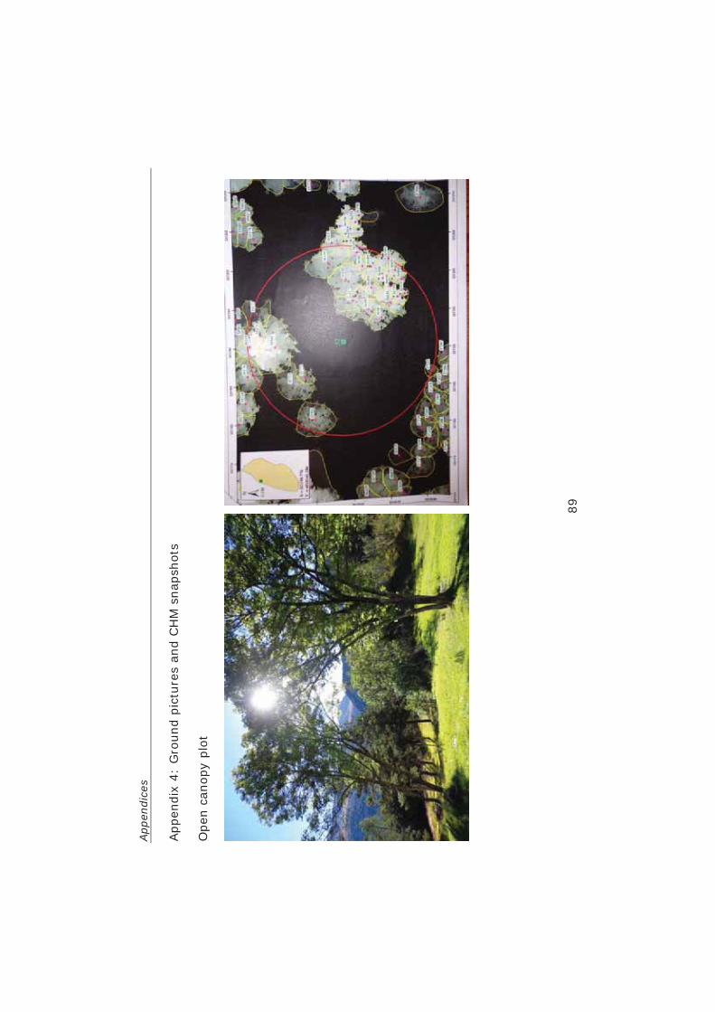
App

endi

ces

89

App

endi

x 4:

Gro

und

pict

ures

and

CH

M s

naps

hots

O

pen

cano

py p

lot

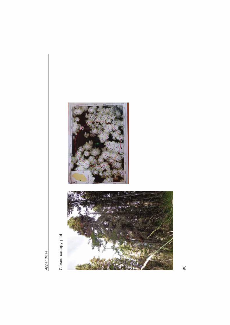
App

endi

ces

90 Clo

sed

cano

py p

lot

Appendices

91

Appendix 5: QQ plots of explanatory variables Clockwise from Top left: Height, Crown Diameter, Intensity coefficient of variation and

Satellite Albedo.

App

endi

ces

92

App

endi

x 6:

With

in-c

row

n sp

ectr

al s

tatis

tics

acro

ss t

he s

peci

es

Key

: PS

_1 –

Pin

us s

ylve

stri

s Ban

d 1

& P

U_1

– P

inus

unc

inat

a Ban

d 1

App

endi

ces

93

Key

: PS

_1 –

Pin

us s

ylve

stri

s Ban

d 1

& P

U_1

– P

inus

unc

inat

a Ban

d 1

App

endi

ces

94

Key

: PS

_1 –

Pin

us s

ylve

stri

s Ban

d 1

& P

U_1

– P

inus

unc

inat

a Ban

d 1

Appendices

95

Appendix 7: Species classification model summaries Logistic Regression based on LiDAR physical parameters glm(formula = Species_code ~ CHM_Height + Crown_D_E + IntCoV, family = "binomial", data = a)

Coefficients: Estimate Std. Error z value Pr(>|z|) (Intercept) 0.64105 0.73191 0.876 0.38110 CHM_Height -0.13769 0.04474 -3.078 0.00209 ** Crown_D_E 0.98795 0.15235 6.485 8.88e-11 *** IntCoV -13.36202 2.22808 -5.997 2.01e-09 *** --- Signif. codes: 0 ‘***’ 0.001 ‘**’ 0.01 ‘*’ 0.05 ‘.’ 0.1 ‘ ’ 1

Logistic Regression based on Spectral parameters glm(formula = Species_code ~ S_Albedo, family = binomial", data = a)

Coefficients: Estimate Std. Error z value Pr(>|z|) (Intercept) -5.6308089 0.7691736 -7.321 2.47e-13 *** S_Albedo 0.0026130 0.0003696 7.070 1.55e-12 *** --- Signif. codes: 0 ‘***’ 0.001 ‘**’ 0.01 ‘*’ 0.05 ‘.’ 0.1 ‘ ’ 1

Logistic Regression based on both physical and spectral parameters glm(formula = Species_code ~ CHM_Height + S_Albedo + IntCoV + Crown_D_E, family = "binomial", data = a)

Coefficients: Estimate Std. Error z value Pr(>|z|) (Intercept) -2.320e+00 1.036e+00 -2.240 0.0251 * CHM_Height -9.912e-02 4.673e-02 -2.121 0.0339 * S_Albedo 1.722e-03 4.158e-04 4.141 3.46e-05 *** IntCoV -1.263e+01 2.289e+00 -5.518 3.43e-08 *** Crown_D_E 6.648e-01 1.691e-01 3.930 8.48e-05 *** --- Signif. codes: 0 ‘***’ 0.001 ‘**’ 0.01 ‘*’ 0.05 ‘.’ 0.1 ‘ ’ 1

Appendices

96

CART based on LiDAR physical parameters

Key: 0 = Pinus uncinata, 1 = Pinus u sylvestris

Key: cp = Complexity point

Appendices

97

CART based on Spectral parameters



Appendices

98

CART based on both physical and spectral parameters



synergy of airborne lidar data and vhr satellite optical - itc

Documents