synthesis a communication network* - … · synthesis of a communication network 349 flows suchthat...

J. Soc. IZCDVST. A,PL. MATH.Vol. 12, No. 2, June, 1964

Printed in U.S.A.

SYNTHESIS OF A COMMUNICATION NETWORK*

R. E. GOMORY AND T. C. HUAbstract. A communication network is a set of nodes connected by arcs.

Every arc has associated with it a nonnegative number called the branchcapacity which indicates the maximum amount of flow that can passthrough the arc. A communication network must have large enough branchcapacities such that all message requirements (which can be regarded asflows of different commodities) can reach their destinations simultaneously.In general, these requirements vary with time. The present paper givesalgorithms for rain-cost synthesis of a communication network which isable to handle simultaneous flows of all time periods.

1. Introduction--Problems of alysis and synthesis the design ocommunication networks. By a communication network we will mean a setof n nodes N and directed arcs linking nodes N and N. Associated withthe arc going from N to N is branch capacity y, and a cost coefficientc,. By a p-q flow, F.q, we will mean the usual flow (see, for example,Ford and Fulkerson [7] with source p and sink q; that is, a set of n(n 1nonnegative numbers x,’q such that

(1) ’ O, ip,q.Xi, Xp’q

(1) of course has the intuitive meaning of requiring that fluid is conservedat all intermediate nodes. The flow value f,q of such a flow is taken to bethe amount of fluid issuing from the source p, so

Xp,s Xr,q

A set of p-q flows will be said to be feasible in a given communication netwith capacity numbers y, if and only if

’q < all i, j.P,q

The two central problems associated with these networks are the prob-lems of analysis and synthesis, both of which involve the notion of require-ment, and which we state first for the case of fixed requirements R,.The problem of analysis" Given a set of n(n 1) nonnegative numbers

R, and a network with capacity numbers y,i, do there exist feasible

Received by the editors September 19, 1963.Thomas J. Watson Research Center, International Business Machines Corpora-

tion, P.O. Box 218, Yorktown Heights, New York. This research was supported inpart by the Office of Naval Research under Contract No. Nonr 3775(00), NR 047040.

348

SYNTHESIS OF A COMMUNICATION NETWORK 349

flows such that

(2) f,q => R,q ?

The problem of synthesis. Given a set of requirements R,q find a net-work having feasible flows satisfying (2) and such that the linear costfunction , ci, yi,. is minimal.

Actually, in a communication net problem there is no one set of require-ments R,q but rather a set R,q(t) varying with a third index, time, thatallows for a changing load on the network. In this article, we will assumethat takes only a finite set of values tl, t2, ts. The degree of difficultyof the problems of analysis and synthesis varies enormously with theassumptions that are made about the R,q(t). The present status of thevarious problems is as follows"

Case 1. R,q independent of t, or all requirements to be met simul-taneously.

Analysis. The basic paper here is Ford and Fulkerson [6]. In this papera linear programming formulation of the problem which resulted in alinear programming problem having an enormous number of columns wasreduced to a reasonable problem by means of a column generating tech-nique which is of the shortest path type. The final problem has m equationsif there are m arcs in the network, and the linear programming is donewith a square m X m matrix. Although the problem treated in [6] is one ofmaximizing total flow rather than meeting a set of requirements, the methodof Ford and Fulkerson requires only minor changes to solve the problemof analysis. A special case where there are only two kinds of flows permitseasy treatment instead of linear programming. See Hu [12].

Synthesis. This problem has an easy solution. Starting with a zerocapacity network, it is only necessary to find the shortest (cheapest) pathbetween the nodes p and q and then give each arc on this path an additionalcapacity R,q. This is repeated for each pair of nodes, the capacities beingadded, to give the minimum cost network. A more economical way ofcarrying out this calculation will be given later in this paper as part ofanother synthesis calculation.

Case 2. Completely time-shared requirements.Here, time is broken up into distinct periods; and during any one period

there is flow between one pair of nodes only. More precisely, there aretimes t,q and R.q(t,q) [.q, and R,q(t,i,) 0 for (i, j) (p, q).

Analysis. This can always be carried out by doing n(n 1) maximumflow calculations of the type of Ford and Fulkerson [5]. However, if thegiven network is symmetric, i.e., y,. y,,, Gomory and Hu [10] showedthat the analysis calculation required only n 1 maximum flow calcula-tions.

350 . :E. GOMORY AND T. C.

Synthesis. A subcase here is especially tractable. If we consider onlysymmetric networks and, in addition, impose a cost function in which allarcs are of equal cost (ci, 1, all i, j), then special rapid methods ofsynthesis become possible; see, for example, Chien [3] and Gomory andHu [10]. However, if the condition ci, 1 is removed, we are again forcedback upon linear programming. The synthesis problem, which can, easilybe posed as a giant linear programming problem involving an enormousnumber of inequalities (rows), was reduced in Gomory and Hu [11] to amore tractable size by means of a row generating technique. Again, itbecame possible to carry out the calculation for an m arc problem using anm m square matrix and auxiliary calculations, that time of the maximalflow type, to produce additional rows when needed.

Case 3. Time varying requirements.Cases 1 and 2 are extreme subcases of this more general problem.Analysis. If we have requirements R,q(t) where is allowed s distinct

values, the problem is merely s distinct repetitions of the analysis problemof Case 1. If the given network can meet the demands R,(t) for eachtime period, then it satisfies the requirements; if it fails at one or moreperiods, it does not meet the requirements.

Synthesis. A special case where the synthesizing network is assumed to bea tree is discussed by Tang [13]. The general case has never been treatedalthough it is, among the problems being reviewed here, the problem ofgreatest practical importance. In this paper we will show that the generaltime varying synthesis problem for an m-arc network can also be reducedto a linear programming calculation involving only one m m squarematrix, plus auxiliary m m linear programming calculations of the Fordand Fulkerson [6] type.

2. Methods of calculation. We will first pose the m-arc synthesis problemwith time varying demands as a completely unwieldy linear programmingproblem. Then we will show how it can be transformed into a problemhaving only m columns, but an enormous number of rows. Finally, we willshow how this enormous number of rows can be dealt with.A) Formulation as a large linear program. Let Y be an m-vector with

each component representing the capacity of an arc in an m-arc networkso that Y represents an entire m-arc network. Let 9Z be an m-vectorrepresenting a network capable of carrying simultaneous flows with flowvalues f,q >- R,q(t). It is easy to show that the networks 9Z form a con-vex (unbounded) po].yhedron in m-space. Consequently, there is a finite listof networks 9z.t such that if 9z can carry the required flows, then

t E i

(3)1 <= hit.


If Y is to meet the requirements for each period, it is necessary and suf-ficient for it to contain a network of the form (3) for each t. So one way ofposing the general synthesis problem is to ask for Y and ki that minimizeC. Y, subject to

X OZi tl t

This formulation involves m(]c -t- 1) rows and an enormous number ofcolumns including one for each 9Zt. To reduce the problem we first use anidea due to Benders [1].B) First reduction. In (4), consider the set of m + 1 inequalities cor-

responding to a particular value t1. Inserting the slack variables to ob-tain equations, we see by Farkas’ theorem that there will exist k satisfyingthe inequalities of (4) for a given Y if and only if

(5) II.(Y, 1) => 0

for all the m -t- 1 vectors II (II, II0) satisfying

(6) n(9k, 1) >_- 0, all i.

Here II1 is a nonnegative m-vector and II0 a nonpositive scalar.The vectors II satisfying (6) also form a convex (unbounded) polyhedron

so that there exists a finite subset IIik, IIq of the II such that all IIsatisfying (5) are positive combinations of these. Consequently, the solva-bility condition (5) which involved all II satisfying (6) can be replaced by

(7) II,.(Y, 1) >_-0, i 1, ..., q(k).

Repeating this for all time periods, we find that a problem formulationequivalent to (4) is

(8) minimize C. Y,

subiect to IIit.(Y, 1) >__ O, i 1, ..., q(t); tl, ..., t,.

This formulation involves only m variables, but generally an enormousnumber of rows, one for each of the IIk.

However, we have not yet specified a computation that will actuallyproduce a finite but adequate list of rows and the actual row coefficients.We turn next to this.

Calculation. We will next consider what is needed to do a calculationusing the formulation (8). We will stress only those parts that are specialto the present problem and will give only a short treatment of the moreroutine simplex steps. A full description is available in [8].We first discuss the dual simplex calculation. This method requires as a

352 i. E. GOMORY AND T. C. HU

preliminary a starting basis that is dual feasible (with its accompanyingnonfeasible Y values) and then the ability to iterate the following steps"

(i) Row selection" Find among the inequalities of (8) one that isnot satisfied by the current Y values.

(9) (ii) Column selection" Use the dual simplex rule.(iii) Gaussian elimination on an inverse matrix only, with the pivot

element the one resulting from the row and column choice in(i) and (ii).

]?’or the primal simplex method we use a starting basis and a Y thatare primal feasible, and the ability to iterate the following steps"

(i) Column selection" Choose for entry in the basis a column thatwill give an improvement.(10) (ii) Row selection" By the primal simplex rule.

(iii) Gaussian elimination on an inverse matrix as in 9(iii).In the dual method, steps (ii) and (iii) are routine steps of the revised

simplex method. (i) requires special consideration. In the primal method,(i) and (iii) are routine with (ii) requiring special treatment. We will con-sider the dual simplex situation first.Dual simplex. Given a fixed dual feasible Y we will solve, for a fixed

tk, the linear programming problem"

Maximize 0 Xk,(11)

subicct to Y __>

If we can solve (11), we will automatically obtain from the simplexcalculation either (i) a 0 >= 1, or (ii) a nonnegative m-vector II1 such that

IIY 0 < 1,(12)

II >= 1, all i.

If in solving 11 we obtain (i) for all t (It 1, s) we have shownthat Y contains a network satisfying the flow requirements for each t.Therefore Y, since it is dual feasible and primal feasible, is the optimalnetwork. If we obtain (ii) for some t; then using the II of 11 to form thevector II (II, -1) we see that

and

II.(Y, 1) < O,

kII. (9, 1) >__ O, all i,

so that we have found in II an unsatisfied inequality of the set (8). Thelist of inequalities II that can be obtained in this way from (11) is finite asthere is one for each basis, yet this list contains an unsatisfied inequality


whenever Y is an infeasible network. Thus the procedure is finite and wedeal with a finite but adequate list of inequalities.Once the inequality has been obtained, the next steps are those of the

ordinary revised dual simplex method. One transforms the inequality bymeans of an inverse, makes the dual simplex column choice by the usualratio test (this is step 9(ii) ), and carries out the Gaussian elimination onlyon the m X m (or with the obiective function (m 1) X (m -[- 1))inverse matrix (step 9 (iii)). One is then ready to iterate by looking for anew unsatisfied inequality.What remains to finish the description of the dual method is to explain

the calculation for solving (11). We do this in a manner closely related tothe method of Ford and Fulkerson [6]. However, instead ot dealing with alinear programming formulation involving a path for each column as in[6], we have a column representing an entire feasible network. This resultsin an economy both in the size of inverse required and in the column generat-ing procedure. To start, we can obtain a feasible solution to (11 using anyfeasible network 9k and kk 0 and then maximize 0. We then obtain forthis problem a set of linear programming prices with an m-vector whosecomponents give a price for each arc. Since we have worked only with9 so far the next question is whether or not there are other feasible net-works 9 which will lead to an increase in 0.Here again, we are facing a very large linear programming problem,

this one having a great many columns, one for each. To select a column,we want to choose the one for which .9 is minimal.

This column can easily be constructed since what we now want is thefeasible network which would most cheaply meet the requirements ofperiod tk if the arc costs were given by II. This is merely the time independentrequirement synthesis problem, and as we remarked in Case 1 of theIntroduction, the synthesis of the cheapest network, which will give usthe new column for the calculation, requires finding the shortest pathbetween each pair of nodes p and q, then using an amount R, of all thearcs of this path, this procedure being repeated for all p, q.However, the path by path construction of the feasible network involves

unnecessary computation since it is overwhelmingly likely that portionsof the same path will be used to connect several different pairs of nodes,and this leads to duplication in the backtracking (or path finding) part ofthe usual shortest path methods. We will next describe a method thatavoids this.As a preliminary, we follow many authors (see, for example, [2]) in

defining as a special matrix product of two m X m matrices Aand B {b,j} the matrix C {c,,j} with

(13) c,. min {a,8 -t- b,,-}.

354 R. :E. GOMORY AND T. C.

For the cheapest feasible network calculation, we first form the m X mmatrix D {d.-} where di.. is the component of giving the price of arci, j. We then form the D2" powers of D by squaring (in the sense of (13))the current power of D and discarding the previous. At the same time, weform and keep successive matrices B, when b.- is an s value for which theminimum in (13) was obtained. After L =< [log2 (n 1)] steps, where [x]indicates the least integer greater than or equal to x, a D2L and accompany-ing BL will be obtained for which 2L ->_ n 1. Of course, the entries inD2L are the shortest path distances from node to node in the network usingdi,. as distance. What we want, however, is a feasible network and forthis we need the B,.Define/L+I {Rp,q(tk)} and define successive/_1 as the matrix that

results from starting with the zero matrix and running through the entriesof/, adding 6,. to the i, /c and lc, j positions of the new matrix. /c is de-termined by b.Then/1 represents the desired cheapest feasible network.To see this, consider the meaning of the various operations involved.

/+ contains the numbers Rp.q(tk) which give the amount of flow theshortest s-step path $ between p and q must carry to satisfy the require-ment./ is derived by adding the amount Rp.q(t) to those two positionsin/ that in the matrix D/2 gave the lengths of the two s/2 step pathswhich combined to form S. Clearly, if S is to carry Rp,q(t), each half of itmust too. This process is then carried back to the halves of the half-paths,etc., until finally the correct weight is assigned to the 1-step paths or arcs.For an example of this calculation, see Tables A1-A5 which treat

5-node example.This is the calculation that is used to generate the improving columns9 for problem 11 ).Primal method. Let us consider the steps outlined under (10) above.

Step (i), column selection, can be done in the usual revised simplex mannerif the Gaussian eliminations on the equations of (8) are recorded as right-multiplications of an (m -t- 1) X (m + 1) matrix. Step (iii) also involvesonly a Gaussian elimination over this matrix. Step (ii), however, involvesfinding out which of the enormous list of inequalities of (7) will be violatedfirst when some currently non-basic variable is increased from its presentlevel of zero.To see how (ii) can be carried out, we first find the effect on the current

values of Y of raising one of the current non-basic variables from its cur-rent value of zero. If we start from (8) and perform Gaussian eliminationsrecorded by right-multiplication of an (m -5 1) X (m -5 1) matrix R,the relation between the (z, Y) and the current non-basic variables T isgiven by (z, Y) R(z, T). If the ith of the non-basic variables is raised to


TABLE A1. Values of [d,’].

@@@@

@ @

0 14 0

2 5

TABLE A2. D and B1

@@@@

[di,i] D

(R)

320

7

(R)

64208

200

@@@@

(R)

01151

0 32 05 31 2

(R)

43401

TABLE A3. D and B2

[di,i] D

(R)

0 25 03 53 5

(R)

54207

@@@@@

(R)

01411

B2

(R)

20512

(R)

24402

a value O, the current Y values Y0 are increased by OY1, where Y1 is the(i A- 1)th column of R. Row selection involves finding the value 0m of0 and the inequality II of (8) which do the following"

(a) Y0 -4- 0m Y1 satisfies all the inequalities of (8) for 0 =< 0 -< 0ma.(b) II.(Y0 zr- OY, 1) < 0 for all0 > 0m.TO find 0 and II we consider for each period the linear programming

problem"

Maximize 0

subject to Yo A- OY >= ii,

356 R.E. GOMORY AND T. C. HU

TABLE A4

(R)(R)(R)(R)

(R)

01010

2

(R)

50001

(R)

40000

(R)

00400

@(R)(R)(R)

TABLE A5

(R)

06000

(R)

00600

which can be rewritten as the problem"

Maximize ’(14) subject to Yo >= OY -!- X’,

1 =< ki.On solving this problem, we will always get a finite maximum for 0 be-

cause an unbounded 0 would give feasible solutions with negative totalcost.On obtaining this finite maximum kOmx by the simplex method, we

automatically get a nonnegative m-vector IIk, and a nonpositive scalarIIok such that

(15) (IIk, IIok) Yo, 1) maxk,and since the scalar product of (-1, II, IIo*) with all the columns on theright of (14) will be nonnegative, we have from the first column

(16) (IIk, II0). Y, O) 1 >__ O.

Multiplying (1.6) by -0 and adding to (15) gives

(17) (II, IIo).[(Yo, 1) + O(Y1,0)] __< Omax .


Yl 4

(a) (b)FIG. 1

FIG. 2

Since, as we remarked above, the scalar product of (IIk, II0k) .9 => 0for all 9, (IIk, II0). (Y, 1) >= 0 is a valid inequality for (8).

All the inequalities of (8) that come from the condition that the networkmust satisfy the requirements of period t are satisfied by Y0 + 0Y1 for0 =< 0 =< 0max, because then Yo + OYI satisfies (14) and so provides afeasible network for time period t. This is a step toward condition (a)above since a portion of the inequalities of (7) are satisfied. Turning nowto the other condition, we see from (17) that

(II,II0).(Y0+0Y, 1) < 0

for 0 > Omx. So condition (b) is fulfilled with II (IIk, II0).If we repeat the calculation (14) for each period tk, and finally choose


Omax min k0max max

then by the reasoning above, condition (a) will be satisfied by Yo - OY1,0 -< 0 __< 0mx, and (IIk, II) is the looked for inequality.

Taking (IIk, II0) as our selected row, we can now proceed with step(iii) of the primal procedure. This completes the description of the primalprocess except for the details of solving (14). However, this is so close tothe procedure for solving (11) as not to require a separate description.

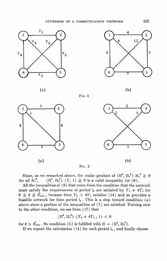
3. Example of the dual method. Consider the network shown in Fig. 1 (a)where the costs c of building unit capacities are as shown in Fig. l(b).There are two time periods with the flow requirements shown in Fig. 2(a)and Fig. 2(b).

In giving the calculation, we will also include a few simple shortcuts inthe calculation. For example, we note in passing that in Fig. l(b), the costof y6 is 12 where the cost of yl and y4 are 4 and 6 respectively. Therefore,the arc y6 will never be used in an optimum solution and we eliminate itfrom the start. This can be done for any arc whose cost equals or exceedsa sum of costs of arcs which form a path connecting the two end nodes ofthe arc.To start the algorithm, we should first test the feasibility of the vector

Y [0, 0, ..., 0] and use the inequality generated by solving (11) tostart the calculation on (8). However, since any inequality, which isnecessary for the network to satisfy, can be used, we can, at the very startof the calculation, get inequalities by utterly simple considerations, thuspostponing the solving of (11) until more refined results are needed. Theinequalities we shall use are that the sum of the branch capacities of arcswhich connect one node to the others must be equal to or greater than thesum of the flow requirements between that node and the others. (This couldalso be done with sets of nodes and sums of requirements.)We start then with Table B1 which represents a portion of (8) and,

except for its top row, will be one inverse. The top row is the cost functionto be minimized, the next five rows are identities, and the last row assertsthat

yly+y-- 8-- v_-> O,

i.e., that node 1 must have arcs totalling at least 8, its requirement sum,connected to it. Note that the positive signs in the top row assure us ofdual feasibility. The notation here is that of [8] and [11].

Using the dual simplex rule, we pivot on the starred element obtainingTable B2 (except for the bottom row). The vl row can now be dropped andreplaced by a new inequality.We next consider node 3, which gives the inequality


TABLE B1

zyl

y.yay4

y5

yl

000000

-8

4-100001"

--y2

50

-10000

700

-1000

6000

-10

-1

40000

--I--I

TABLE B2

z

Yly2

YY4Y5

--3280000

--8

4--10000

50

--i000

-1

700

-100

-1

2100

-10

-y5

01000

-1

-1"

TABLE B3

z

YY2YYYv

--8170701

--8 --1

-y2

01

-11

-10

-2* 1 0 0

(18) --8 -- y: -k Y3 -- Y5 => O.

To express this inequality in terms of the current non-basic variables weturn Table B2 into the inverse by replacing the top row by 1, 0, 0, 0, 0, 0)and then multiply the row vector (- 8, 0, 1, 1, 0, 1 ). This gives (18) in theform needed. It is placed in the position where the vl row was (see TableB2) and another pivot step is then made on the starred element.We proceed in this way, considering nodes 4 and 2, with the obvious asso-

ciated inequalities y q- y 7 3 _-> 0 and y q- y 7 v _-> 0 andobtuin Table B3 (except for the bottom row).

360 . E. GOMORY AND T. C. HU

TABLE B4

zYly2

Y3Y4Y5v6

--8134341

--3

0

01

TABLE B5

z

Yly2

Y3Yy5

--85.5

34

At this point, these simple inequalities are satisfied and we must gothrough the full auxiliary calculation solving (11) to obtain a new in-equality.At the beginning the prices (which appear in the top row of Table C1) are

all zero so any feasible network provides an improving column such asthe one headed 91. After pivoting, we have a nonzero price, and thecheapest network calculation described earlier gives a feasible network,(4, 0, 3, 4, 5), which, expressed in terms of the current variables, gives theleft column in Table C2. We proceed through another pivot step and twomore improving networks as shown in Tables C3 and C4 before reachingTable C5. Then the feasible network calculation shows that for aII (0, , 0, , ) there is no feasible network with II. < 1, althoughIIY < 1. This gives us our new inequality IIY => 1 or equivalently

--9-t-y2-y4y5 v5 >= 0,

which is transformed to become the bottom row of Table B3. After pivot-ing, we obtain Table B4.The auxiliary calculation (11) now shows that the requirements for

period 1 are now met and we must now do the auxiliary calculation for therequirements of period 2. Of course, the Y values in Table B4 which givethe cheapest network satisfying the first period requirements could have


been obtained much more cheaply and easily by a single feasible networkcalculation. However, it is necessary to obtain the inequalities representedby the rest of the matrix if one is to proceed further.

TABLE C1

-i34*341

S Sz

0 00 01 00 10 00 0

000010

TABLE C2

2

-14034*5

S

TABLE C3

-I41"7

--I9

000100

TABLE C4

4

-I70709*

S S

01 -1/40

0 0

S Y

0 00 70 00 70 01 1

362 2. E. GOMORY AND T, C. HU

TABLE C5

7 $3

F. 3

An auxiliary calculation like that of Tables C1-C5 yields pricesII (-r6, 0, o, 0, 1%) and a 0 of only . Hence, the inequality

which is used in Table B4 to obtain Table B5. The auxiliary calculationsfor both periods 1 and 2 give values of 0 >= 1 so this is a feasible, and there-fore optimal, network. Thus, the cheapest network for our requirementsis shown in Fig. 3 and given by

Y= (, , 3, 4, )

with cost 85.5.Primal calculation. We will redo the example using the primal method.

This approach has the advantage of giving a feasible network at all times,so that calculation can be stopped if progress is too slow.The first step is to get a starting feasible solution. This is easily done by

giving the arc connecting nodes i and j a capacity equal to maxt Ri.j(t).Applying this to our example gives a starting solution Y (3, 4, 3, 4, 2, 3 ).However, iust as before, there is no gain in considering an arc such as y6

whose cost is greater than that of an alternate path connecting its endpoints. So we will rule out y6 and fulfill its requirement by adding 3 unitsto the alternate path yly4 to give the starting feasible five-arc networkY (5, 4, 3, 4, 2).

SYNTIIESIS OF A COMMUNICATION NETWORK 363

TABLE D1

Z

yl

y3

y4

y5

-9354342

--410000

--501000

-700100

--600010

--400001

TABLE E1

X1

1000000

0000100

0000010

000000

-1

-1001000

TABLE E2

X1

1 00 10 00 00 00 00 0

0000100

034341

-1

-1001"000

To obtain a starting basis, we introduce the variables u, i 1,which are unrestricted in size and are defined by

,5,

yl 5 Ul, y2 4 u., y3 3 u3,

y4 4- m, and y5 2- us.

This gives the starting array of Table D1. Clearly, a better solution can beobtained by increasing u3 from its current value of 0 to some value 0.We will find the largest possible value of 0 and the limiting inequality bysolving the system (14) with Yo (5, 4, 3, 4, 2) and Y1 (0, 0, 1, 0, 0).


TABLE E3

X2

--300

--33*31

1000000

Sz $4

1 00 00 0

00 10 00 0

334341

--1

TABLE E4

X2

00001"00

Sz $4

1 10 00 01

0 --10

0 70 30 40 70 ---30 --TABLE D2

Z

Yly2

YY4YYl

-93543420

--4

00000

-5010000

-700

001"

--600010

--40000

0

TABLE D3

Z

yl

YY.YY/)2

-9354342

--4100000

--5010001"

700

-100

-1

100

-1

0-1

-4000011


TABLE D4

z

YlY2YaY4y5

--88533420

--4100000

--t2

50

-1000

-1

201

--1001

--401

--1102*

10

--10010

TABLE D5

z

YlY2YY4Y

--8853342

--410000

40

0

20

0

10

-1001

TABLE D6

z

Yly2

YYy5

V5

--88533421

4--i0000

--i

1

00

--h

2

01

4

0--1

--5+1+100

-12

For the solution of (14), which is of course again a linear programmingproblem, we need a starting basis, i.e., for a starting value of 0 (which willbe zero) we need to express Yo nt OY1 as a sum of feasible networks andslacks. This yields the starting Table El.

Pivoting on the starred element now yields an increase in 0 and Table E2.The 0 column now is an improving one so we pivot on that column giving,

except for the left-most column, Table E3. Next, using the linear program-ming prices from the top row, we do the special matrix calculation to get

366 R, Eo GOMORY AND T. C. I-IU

TABLE D7

z

YYYaYYv5

85.5

34

0

1

00

5

FG. 4

5

FIG. 5

5

a cheapest feasible network which turns out to be (3, 4, 0, 7, 4). This, afterbeing enlarged to (0, 3, 4, 0, 7, 4, 1 by adding its coefficients in the top andbottom rows, is updated to become the left-most column in Table E3.Pivoting on the starred element gives Table E4.

cannot be increased any more as our column generating procedureshows. Thus, the inequality

(19) -7 +y3+y4 vl_>- 0

SYNTHESIS OF A COMMUNICATION NETVORK 367

TABLE F1. First period requirements

(9 x(R)(R)(R)(R)(9(R)

(R)@

12X

639X

3963X

45264X

709

1102X

7432663X

3475213

12X

9558914417X

TABLE F2. Second period requirements

(R)

(R)

(R)

@

(R)

X7231870143

X14

15

o17

X672941714

X61223124

X317819

11112

X4197

X43

X8

obtained from the prices appearing in Table E4 is the binding inequalityamong those that insure the continued first period feasibility of our net-work. Ordinarily we would repeat this calculation using second periodfeasible networks to find the binding inequality among those that insuresecond period feasibility and then choose the one with the smaller 0. How-ever, in this case with Om already 0, this second step is unnecessary.

(19) is adjoined to Table D2 and a primal pivot step is made.The result (except for the bottom row) appears in Table D3. Now a

further improving column is (0, 1, 0, 0, 0). To find O and the binding con-straint, the calculation of (14) is repeated with Y0 (5, 4, 3, 4, 2) andY1 (0, 1, 0, 0, 0). This time, both periods are considered and the bind-ing inequality, which comes from the first period requirement, is

(20) -8 +y2 +y3 +y5 v2->_ 0,with Omax 1. Updating this inequality gives the bottom row in TableD3, and a primal pivot step produces the new network of Table D4 andFig. 4.

368 t, l. GOMORY AND T, C. ttU

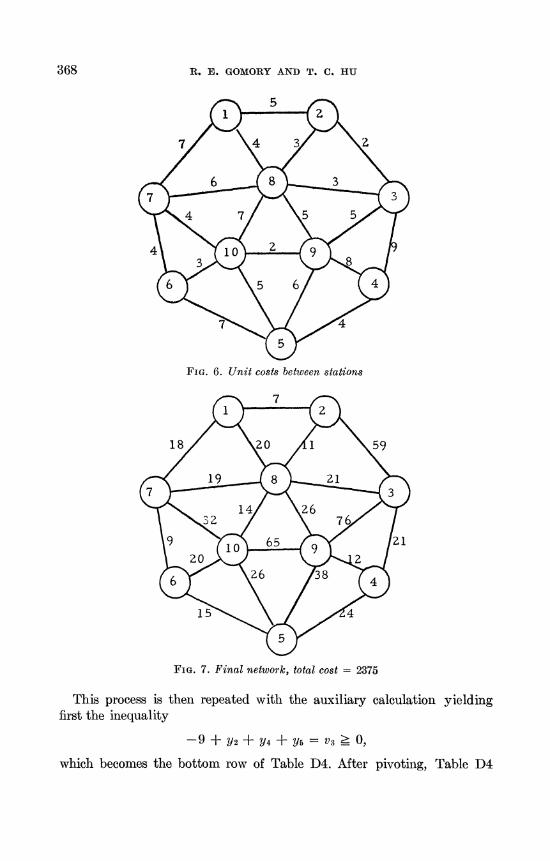
FI. 6. Unit costs between stations

FIG. 7, Final network, total cost 2375

This process is then repeated with the auxiliary calculation yieldingfirst the inequality

--9 --y2+ Y4 -- Y5 va >_- O,

which becomes the bottom row of Table D4. After pivoting, Table D4


becomes Table D5. The auxiliary calculation then yields

-10 - y+ y-t- y- 4_>- 0,

which updated appears in the bottom of Table D5. The next pivot yieldsTable D6. The next inequality is a recurrence of

-7 y -t- y. > 0.

Pivoting yields Table D7. In Table DT, there is no longer any improvingcolumn so the optimal network has been found and is the same as theone given by the dual calculation.

4. A larger example. A ten-node twenty-arc network was considered.Unit costs are given in Fig. 6; the requirements for the two periods involvedappear in Tables F1 and F2. The problem was run on the IBM 7094 usingthe dual method. After a run of ten minutes, the minimum synthesisshown in Fig. 7 was obtained.

REFERENCES

[1] J. F. BENDERS, Partitioning in mathematical programming, Thesis, UtrechtUniversity, 1960.

[2] C. BERGE, Theory of Graphs, trans. Alison Doig, John Wiley, New York, 1962,pp. 138-139.

[3] R. T. CHIEN, Synthesis of a communication net, IBM J. Res. Develop., 4 (1960),pp. 311-320.

[4] J. FARKAS, Uber die Theorie einfachen Ungleichungen, J. Reine Angew. Math.,124 (1901), pp. 1-27.

[5] L. R. FORD, JR., AND D. n. FULKERSON, A simple algorithm for finding maximalnetwork flows and an application to the Hitchcock problem, Canad. J. Math.,9 (1957), pp. 210-218.

[6], A suggested computation for maximal multi-commodity network flows,Management Sci., 5 (1958), pp. 97-101.

[7] ------, Flows in Networks, Princetoa University Press, Princeton, 1962.[8] I. E. GOMORY, An algorithm for integer solutions to linear programs, Recent

Advances in Mathematical Programming, McGraw-Hill (ed. Graves andWolfe), New York, 1963.

[9] --, Large and non-convex problems in linear programming, Proceedings ofSymposia in Applied Mathematics, Vol. 15, Amer. Math. Soc., 1963.

[10] R. E. GOMOttY AND T. C. Hv, Multi-terminal network flows, this Journal, 9 (1961),pp. 551-570.

[11] ------, An application of generalized linear programming to network flows, thisJournul, 10 (1962), pp. 260-283.

[12] T. C. Hu, Multi-commodity network flows, Operations Res., 11 (1963), pp. 344-360.

[13] D. T. TANG, Communication Networks with Simultaneous Flow Requirements,IEEE Trans. Circuit Theory, CT-9 (1962).

synthesis a communication network* - … · synthesis of a communication network 349 flows suchthat...

Documents