system identification of a steam distillation pilotscale

IJRET: International Journal of Research in Engineering and Technology eISSN: 2319-1163 | pISSN: 2321-7308

__________________________________________________________________________________________

Volume: 03 Issue: 01 | Jan-2014, Available @ http://www.ijret.org 144

SYSTEM IDENTIFICATION OF A STEAM DISTILLATION PILOT-

SCALE USING ARX AND NARX APPROACHES

Haslizamri Md Shariff1, Mohd Hezri Fazalul Rahiman2, Ihsan Yassin3, Mazidah Tajjudin4 1Asst. Lecturer, 2, 3, 4Lecturer, Faculty of Electrical Engineering, Universiti Teknologi MARA, Shah Alam Malaysia

Abstract This paper presents steam temperature models for steam distillation pilot-scale (SDPS) by comparing Pseudo Random Binary Sequence (PRBS) versus Multi-Sine (M-Sine) perturbation signal Both perturbation signals were applied to nonlinear steam distillation system to study the capability of these input signals in exciting nonlinearity of system dynamics. In this work, both linear and nonlinear ARX model structures have been investigated. Five statistical approaches have been observed to evaluate the developed steam temperature models, namely, coefficient of determination, R2; auto-correlation function, ACF; cross-correlation function, CCF; root mean square error, RMSE; and residual histogram. The results showed that the nonlinear ARX models are superior as compared to the linear models when M-Sine perturbation applied to the steam distillation system. While, PRBS perturbation exhibit insufficient to model nonlinear system dynamic Keywords: SDPS, PRBS, M-Sine, ARX, R2, ACF, CCF, RMSE

---------------------------------------------------------------------***------------------------------ -------------------------------------------

1. INTRODUCTION

Steam distillation is one of the earlier and common separation techniques in chemical manufacturing [1], [2]. In 1991, estimated that 40,000 distillation columns operate in the United State alone to produce the essential oil, comprising 40% of all energy usage in the refining and commodity chemical manufacturing sector [3]. In Malaysia, the essential oil is produced using steam distillation techniques and the demand of essential oil is increasing every year, nevertheless the production of steam distillation process has not been explored widely [2], [4]. Only few number of research efforts have been reported in improving the oil extraction techniques since the past three decades [2]. In real time process, most of the chemical engineering processes are nonlinear in their dynamics [1], [5], [6], [7], including the behavior of the distillation column [1], [5], [7], [8]. Until today, almost all the works related to identification of steam distillation column still using linear model to represent the process dynamic [1], [2], [9], [10], [11]. Unfortunately, the linear identification is limited for a given input range [7], [12], [13], [14]. In the last decades, there has been a tendency towards nonlinear modeling in various application areas; encourage with technological innovations has resulted less limitations on the computational, memory and data-acquisition level, making nonlinear modeling a more feasible and flexible choices [7], [12], [13], [14] To be more feasible and flexible, a systematic modeling is required to describe a phenomenon of interest with improved understanding for the purposes of simulation, prediction and

control. In order to develop systematic model, system identification is under control engineering field is offer how to build the dynamics of a system as a set of mathematical model based on the observation of input and output data [15], [16]. The mathematical model created is capable of relating the system output for any given input in such a way that it can even predict the future of the system. The primary goal of system identification is to reduce errors between model and true system [17]. The model is capable of facilitating the controller and optimizing the system in which the traditional control technique find a difficult to achieve [12], [14]. 2. SYSTEM IDENTIFICATION

System identification research and applications has been growth up and it was recognized as important tool in numerous fields. Nowadays, system identification is getting more attention owing to widespread development of sophisticated and efficient algorithms, coupled with the advancement of digital processing and computing. The derivation of a relevant ‘system description’ from the observed data is termed as system identification, and the resultant system description as a ‘model’ [1]. Scientifically, system identification deals with the problem of building mathematical models of dynamical systems to describe the underlying mechanism of the observed data of the systems [1]. In order to design and implement high performance of control system the dynamic model is required. The obtained model must be validated to verify whether the model is preciseness before implemented. This is done by comparing the output of the


__________________________________________________________________________________________


obtained model and the output of the plant using part of the experimental data that has been reserved for this purpose [18]. There are two main types of empirical models: linear models and nonlinear models [12]. Linear models provide an appropriate representation of the process in a small neighborhood of an operating point. However, when the process is operated outside this constrained region, the model predictions will not accurate. Other offer is nonlinear model, where tend to capture more accurately the process behavior, making the adequate for controlling a real process in a wide region of operation. The distillation column are widely used in chemical processes and exhibit nonlinear dynamic behavior [6], [19], [20]. In recent year, the has been an increasing interest in modeling of heating process especially in distillation column to extract the essential oil where the linear model become most common in industrial application [21]. Unfortunately, linear approximations are only valid for a given input range [12]. The nature of the chemical industrial itself, economics of operation and the unit operation themselves, imposes additional requirements on process models [7]. The need for improved product quality while maintaining a safe and economical operation requires that plants be operated over a broad range about the nominal operating point [7]. This leads to plant operation close to constraints and excites nonlinearities in system behavior. In distillation column exhibit symmetric output changes to symmetric input changes (reflux ratio) [22]. In addition, reacting system often display nonlinearities arising due to the reaction mechanism or due to the non-isothermal nature of the rate constant [7]. This nonlinear behavior presents a difficulty for linear controller due to their limitations [6]. Thus nonlinearity is integral part of chemical process operation and must be accounted for while developing nonlinear models [7]. From logical perspective it would seem that a nonlinear system would require a nonlinear model to fully exhibit its characteristics [23]. However, common practice most that a linear model will be the first choice with which to identify a model of a nonlinear system process, and that this course of action often leads to satisfactory model fit for its purpose [23]. In the case of approximation linear model of nonlinear system, it can be validate by compare linear and nonlinear model to identify which model display the best result. To ensure the system process able to fully exhibit its characteristics, persistently exciting perturbation signal is required. Otherwise, comparison between both model obtained will not exhibit significant improvement on this effort. The main objective of this research is to reveal a solution to this problem.

3. PERTURBATION SIGNAL

System identification deals with the problem of how to estimate the model of a system from measured input and output signals [24]. The system can be linear or nonlinear depending on type of the system, linear or nonlinear model can be estimated. The most important thing is perturbation signal injected to a system must have sufficient excitation (enough fluctuating) of desired effect in order to measure and describe some property of the system dynamic. In nonlinearity identification of system dynamic, perturbation signal must be persistently exciting (or enough fluctuating) in order to excite the full range of nonlinearity process dynamics [7]. For linear system, deterministic PRBS have been commonly used. However PRBS input is insufficient to exhibit the nonlinearity behavior of dynamic system. It is in agreement with the claimed by [14], [25], [26] that the PRBS consists of only two levels, the resulting data may not provide sufficient information to identify nonlinear behavior [1], [14], [26], [27]. These signal cannot excite certain nonlinearities, so that more input levels in the sequence are necessary [7], [17], [26], [27]. In addition, the magnitude of PRBS is too large may bias in estimation of linear kernel. In this research, NARX model will be developed with persistently exciting required perturbation signal; M-level PRS. The objective of using M-level PRS input is to study this signal capability to excite the nonlinearity of system dynamic. The advantages of these signal operate at many operating levels and provide the possibility of identifying nonlinearities behavior, or of identifying linear behavior in the presence of nonlinearities [25], [26]. 4. MODEL STRUCTURE SELECTION

4.1 ARX Model

An ARX model is one of the linear model in system identification. The ARX model comprising of past output and exogenous input variable is represented as past input data. The ARX model is among the simple models for linear process and it is easy to be implemented. The ARX model is written as [15]:

)()(

1)(

)(

)()( te

qAtu

qA

qBqty nk += −

(1) Where the polynomial A(q) and B(q) are defined by:

nana qaqaqA −− +++= ...1)( 1

1 (2)

nbnbqbqbbqB −− +++= ...)( 1

10 (3)


__________________________________________________________________________________________


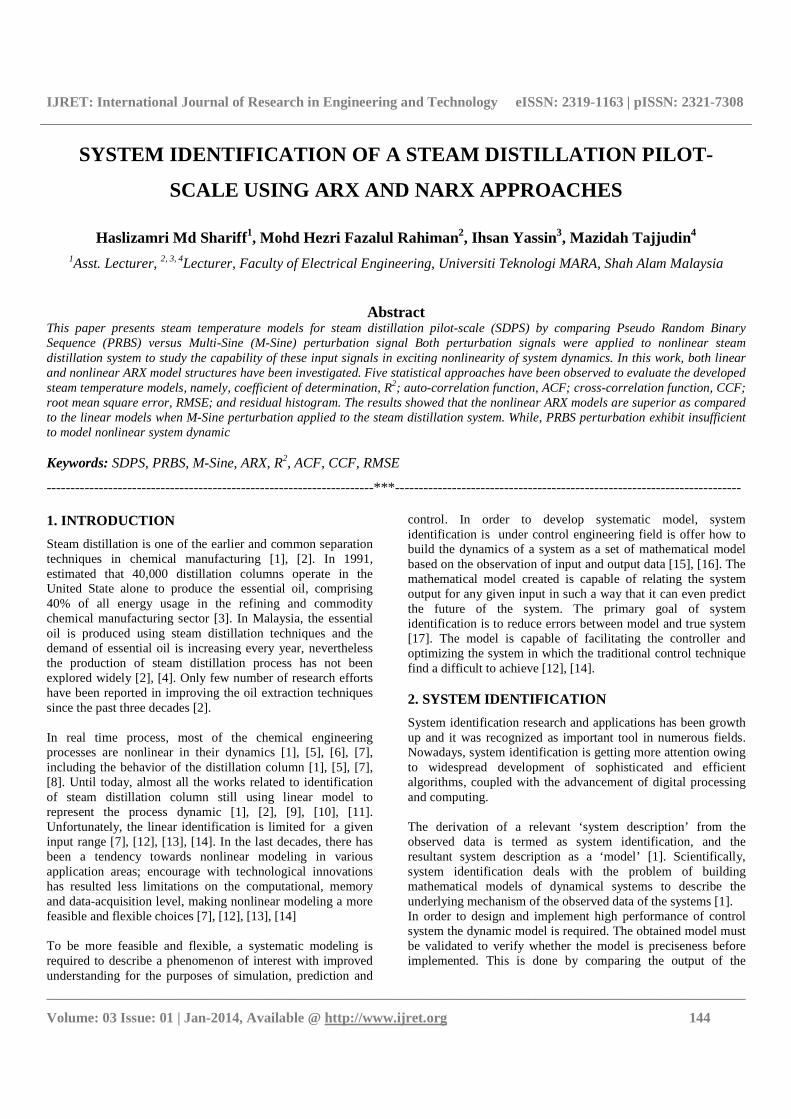
Where A(q) and B(q)to be estimated which represent the overall system dynamic andq-1as time shift operator and this q description is completely equivalent to the Z-transform form i.e. q corresponds to z [15] and the signal flow can be realized as :

Fig 1: The ARX model structure 4.2 NARX Model

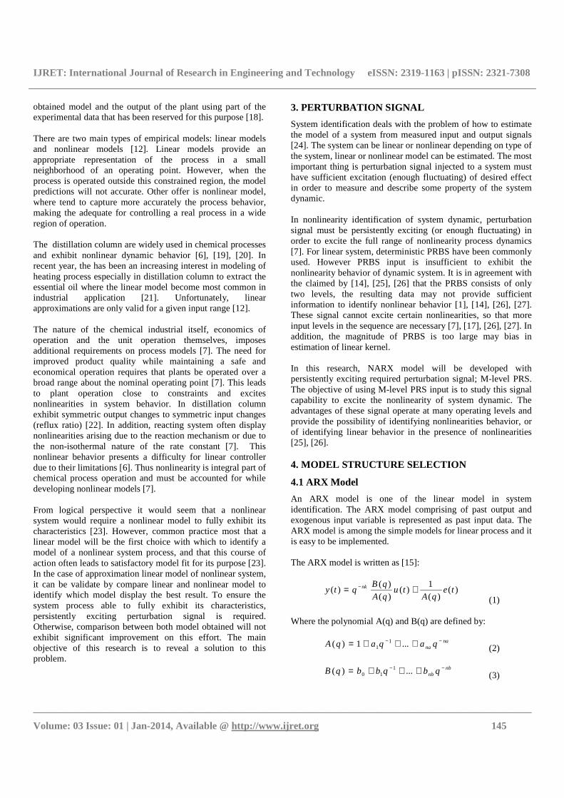
Most dynamical systems can be better represented by nonlinear models [12], [28], where the models are able to describe the global behavior of the system over the whole operating range. It contrast with linear models are only able approximate the system around a given operating point [28]. One of the most frequent studied classes of nonlinear models are called block-oriented models, which consist of the interconnection of linear blocks and nonlinear block [29]. There are many approach of nonlinear system identification methods, where the methods are different owing to varied positioning of interconnection, types of linear and nonlinear functions [28]. One of the method is nonlinear auto regressive with exogenous input (NARX) model, where the nonlinearity estimator block is combine with linear ARX and nonlinear function in parallel, maps the regressor output to the model output. The structure of NARX shown in figure 2:

Fig 2: Structure Of Nonlinear Auto-Regressive With Exogenous Input (NARX)

The equation of NARX model can be written as:

(4)

Where y(t) is output, r are the regressors, u is input and L is an autoregressive with exogenous (ARX) linear function. D is a scalar off-set and g(Q(u-r)) represents output of nonlinear function and Q is projection matrix that makes the calculations well-conditioned. The NARX model is suitable for modeling both the stochastic and deterministic components of a system and is capable of describing wide variety of nonlinear system [2]. 5. MODEL VALIDATION

Model validation is final stage, where the stage is mandatory step to decide the identified model is accepted or not[30]. The purpose of model validation is to verify whether the identified model fulfill the modeling requirement for a particular application. In achieving good estimated model, it is necessary to distinguish between the lack of fit between model and data due to random processes and that due to lack of model complexity.In most statistical tools, a measure of model fit is determine by coefficient of determination, R2 [31]. The R2 given by;

(5) The RMSE is used to assess the forecasting performance of a predictor. As the prediction accuracy increases, the RMSE decreases [32]. The RMSE is given by;

(6) The RMSE also used to evaluate the performance of a predictor over another by calculating the improvement achieved. It is useful especially when calculating the significant improvement achieved by a nonlinear model over a linear model [33]. The improvement calculation is given as follows;

(7) The ACF is a mathematical function that is used frequently in signal processing for analyzing series of values such as time-domains signal [2].Relative to PSD, ACF is its time-domain counterpart [34]. The ACF reveal the strength of relationship between two observation as a function of the time separation between them, or in other words, the cross-correlation of a signal with itself. ACF is useful in investigating repeating patterns in a signal such as determining the presence of a periodic signal which has been buried by noise. This capability makes ACF very important tools in determining the whiteness of stochastic signal. The ACF and CCF respectively given by;

+ +

u y

e

Regressor u(t), u(t-1),… y(t), y(t-1),…

Nonlinear g(.)

linear (LTI)


__________________________________________________________________________________________


(8)

(9)

where the terms of and are the average residuals and

inputs respectively. is the lag and it is common to investigate the ACF and CCF between lag ±20 [35]. The power spectral density (PSD) of a signal is a description of the distribution of the signal power of the signal versus frequency [34]. The PSD is capable of capturing the frequency content of a stochastic process. The unit of PSD is commonly expressed in power/frequency (dB/Hz). The PSD of a signal can be estimated by using periodogram. Residual which is also known as prediction error describes the

error in the fit of the model to the observation . The residuals can be used to provide the information about the

adequacy of the fitted model[31]. Residual of prediction is given

- ;i = 1,2,3,….,N

Where is the observed output, is the predicted output, iis

the sequence and N is the number the data. From a time –series plot of residuals, if the residual is randomly distributed around zero, it indicated that the estimated model describes the observed data well[36]. Histogram is a method to summarize a data distribution into several intervals and the number of data points in each interval is represented as bar length[37]. It is sometimes referred to as frequency distribution[38]. Based on the time-series of

residual ., a histogram can be plotted. The residual are expected to be normally distributed because the normal distribution often provides an adequate approximation to the distribution of many measured quantities. 6. EXPERIMENTAL DESIGN

6.1 Experimental Set-Up

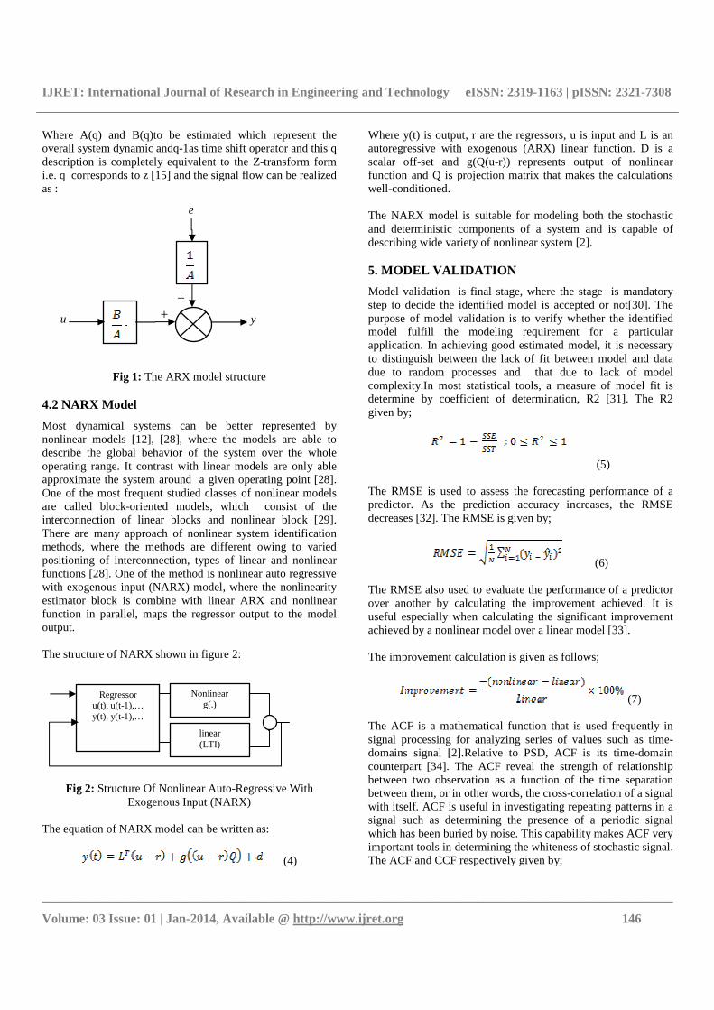
The steam distillation pilot plant using 1500W coil-type heater to generate steam. The heater is immersed in 10liters of water for 2000 seconds. Two (2) resistive temperature detectors (RTD) PT-100 were installed. The primary RTD used to monitor water temperature in the column, and secondary RTD to monitor steam temperature that was installed 30cm from steam outlet. The output from both RTDs is resistance are converting to voltage by using signal converter that produced output within 1V to 5V for temperature range varies from 0°C

to 100°C. Power controller used to control heater are manipulated by providing control signal.

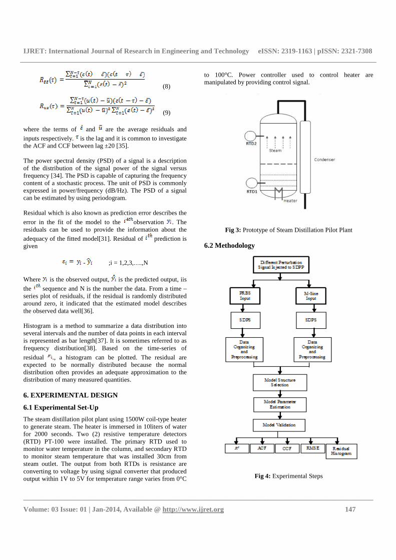
Fig 3: Prototype of Steam Distillation Pilot Plant 6.2 Methodology

Fig 4: Experimental Steps


__________________________________________________________________________________________


6.3 Data Analysis

6.3.1 PRBS Perturbation

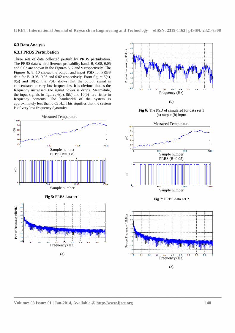
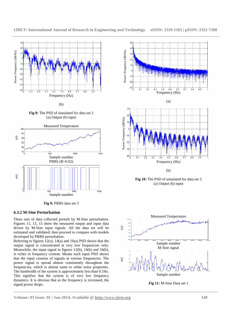
Three sets of data collected perturb by PRBS perturbation. The PRBS data with difference probability band, B; 0.08, 0.05 and 0.02 are shown in the Figures 5, 7 and 9 respectively. The Figures 6, 8, 10 shows the output and input PSD for PRBS data for B; 0.08, 0.05 and 0.02 respectively. From figure 6(a), 8(a) and 10(a), the PSD shows that the output signal is concentrated at very low frequencies. It is obvious that as the frequency increased, the signal power is drops. Meanwhile, the input signals in figures 6(b), 8(b) and 10(b) are richer in frequency contents. The bandwidth of the system is approximately less than 0.05 Hz. This signifies that the system is of very low frequency dynamics.

Measured Temperature

Sample number PRBS (B=0.08)

Sample number

Fig 5: PRBS data set 1

Frequency (Hz)

(a)

Frequency (Hz)

(b)

Fig 6: The PSD of simulated for data set 1

(a) output (b) input



Sample number


Frequency (Hz)

(a)

Po

wer

/ Fre

quen

cy (

dB

/Hz)

y(

t)

u(t

) u(t

) y(

t)

Po

wer

/ Fre

quen

cy (

dB

/Hz)

Po

wer

/ Fre

quen

cy (

dB

/Hz)


__________________________________________________________________________________________


Frequency (Hz)

(b)


(a) Output (b) input



Sample number


Frequency (Hz)

(a)

Frequency (Hz)

(b)



6.3.2 M-Sine Perturbation

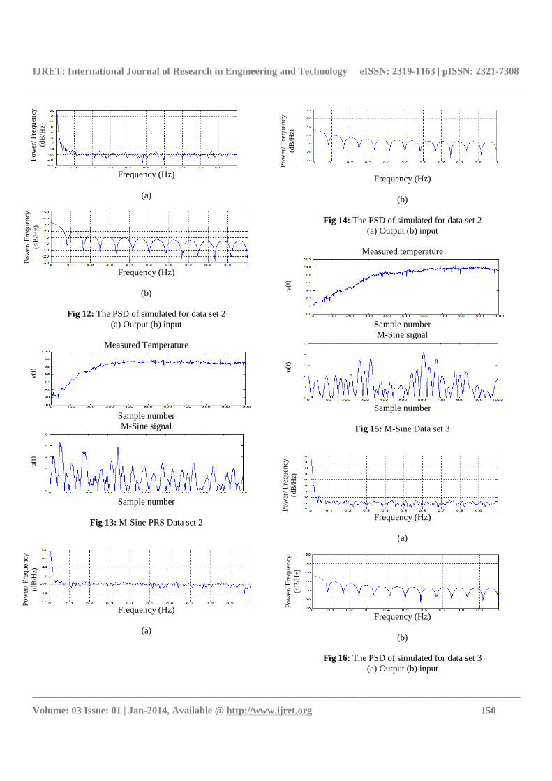
Three sets of data collected perturb by M-Sine perturbation. Figures 11, 13, 15 show the measured output and input data driven by M-Sine input signals. All the data set will be estimated and validated; then proceed to compare with models developed by PRBS perturbation. Referring to figures 12(a), 14(a) and 16(a) PSD shows that the output signal is concentrated at very low frequencies only. Meanwhile, the input signal in figures 12(b), 14(b) and 16(b), is richer in frequency content. Means each input PSD shows that the input consists of signals at various frequencies. The power signal is spread almost consistently throughout the frequencies, which is almost same to white noise properties. The bandwidth of the system is approximately less than 0.1Hz. This signifies that the system is of very low frequency dynamics. It is obvious that as the frequency is increased, the signal power drops.


Sample number M-Sine signal

Sample number

Fig 11: M-Sine Data set 1

Po

wer

/ Fre

quen

cy (

dB

/Hz)

Po

wer

/ Fre

quen

cy (

dB

/Hz)

Po

wer

/ Fre

quen

cy (

dB

/Hz)

y(t)

u

(t)

y(t)

u

(t)


__________________________________________________________________________________________


Frequency (Hz)

(a)

Frequency (Hz)

(b)





Sample number

Fig 13: M-Sine PRS Data set 2

Frequency (Hz)

(a)

Frequency (Hz)

(b)

Fig 14: The PSD of simulated for data set 2 (a) Output (b) input

Measured temperature


Sample number

Fig 15: M-Sine Data set 3

Frequency (Hz)

(a)

Frequency (Hz)

(b)



Po

wer

/ Fre

quen

cy

(dB

/Hz)

Po

wer

/ Fre

quen

cy

(dB

/Hz)

Po

wer

/ Fre

quen

cy

(dB

/Hz)

u

(t)

y(t)

u

(t)

Po

wer

/ Fre

quen

cy

(dB

/Hz)

P

ow

er/ F

requ

ency

(d

B/H

z)

Po

wer

/ Fre

quen

cy

(dB

/Hz)

y(

t)


__________________________________________________________________________________________


7. RESULTS

7.1 Results for PRBS Data

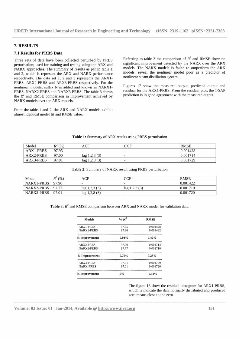
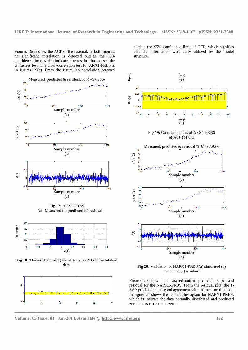
Three sets of data have been collected perturbed by PRBS perturbation; used for training and testing using the ARX and NARX approaches. The summary of results as per in table 1 and 2, which is represent the ARX and NARX performance respectively. The data set 1, 2 and 3 represents the ARX1-PRBS, ARX2-PRBS and ARX3-PRBS respectively. For the nonlinear models, suffix N is added and known as NARX1-PRBS, NARX2-PRBS and NARX3-PRBS. The table 3 shows the R2 and RMSE comparison in improvement achieved by NARX models over the ARX models. From the table 1 and 2, the ARX and NARX models exhibit almost identical model fit and RMSE value.

Referring to table 3 the comparison of R2 and RMSE show no significant improvement detected by the NARX over the ARX models. The NARX models is failed to outperform the ARX models; reveal the nonlinear model poor as a predictor of nonlinear steam distillation system. Figures 17 show the measured output, predicted output and residual for the ARX1-PRBS. From the residual plot, the 1-SAP prediction is in good agreement with the measured output.

Table 1: Summary of ARX results using PRBS perturbation

Model R2 (%) ACF CCF RMSE ARX1-PRBS 97.95 - - 0.001428 ARX2-PRBS 97.00 lag 1,2,3 (3) - 0.001714 ARX3-PRBS 97.01 lag 1,2,8 (3) - 0.001729

Table 2: Summary of NARX result using PRBS perturbation

Model R2 (%) ACF CCF RMSE NARX1-PRBS 97.96 - - 0.001422 NARX2-PRBS 97.77 lag 1,2,3 (3) lag 1,2,3 (3) 0.001710 NARX3-PRBS 97.01 lag 1,2,8 (3) - 0.001720

Table 3: R2 and RMSE comparison between ARX and NARX model for validation data.

______________________________________________________ Models % R2 RMSE

______________________________________________________ ARX1-PRBS 97.95 0.001428 NARX1-PRBS 97.96 0.001422

--------------------------------------------------------------------------------- % Improvement 0.01% 0.42%

--------------------------------------------------------------------------------- ARX2-PRBS 97.00 0.001714 NARX2-PRBS 97.77 0.001710

--------------------------------------------------------------------------------- % Improvement 0.79% 0.23%

--------------------------------------------------------------------------------- ARX3-PRBS 97.01 0.001729 NARX-PRBS 97.01 0.001720

--------------------------------------------------------------------------------- % Improvement 0% 0.52%

______________________________________________________

The figure 18 show the residual histogram for ARX1-PRBS, which is indicate the data normally distributed and produced zero means close to the zero.


__________________________________________________________________________________________


Figures 19(a) show the ACF of the residual. In both figures, no significant correlation is detected outside the 95% confidence limit, which indicates the residual has passed the whiteness test. The cross-correlation test for ARX1-PRBS is in figures 19(b). From the figure, no correlation detected

outside the 95% confidence limit of CCF, which signifies that the information were fully utilized by the model structure.

Measured, predicted & residual. % R2=97.95%

Sample number

(a)

Sample number

(b)

Sample number

(c)

Fig 17: ARX1-PRBS (a) Measured (b) predicted (c) residual.

ε(t)

Fig 18: The residual histogram of ARX1-PRBS for validation

data.

Lag (a)

Lag (b)

Fig 19: Correlation tests of ARX1-PRBS

(a) ACF (b) CCF

Measured, predicted & residual % R2=97.96%

Sample number

(a)

Sample number

(b)

Sample number

(c)

Fig 20: Validation of NARX1-PRBS (a) simulated (b) predicted (c) residual

Figures 20 show the measured output, predicted output and residual for the NARX1-PRBS. From the residual plot, the 1-SAP prediction is in good agreement with the measured output. In figure 21 shows the residual histogram for NARX1-PRBS, which is indicate the data normally distributed and produced zero means close to the zero.

y-ha

t (˚C

)

Rµε

(t)

ε(

t)

Rεε

(t)

y(

t) (

˚C)

y-

hat (

˚C)

Fre

que

ncy

y(t)

(˚C

)

ε(t)


__________________________________________________________________________________________


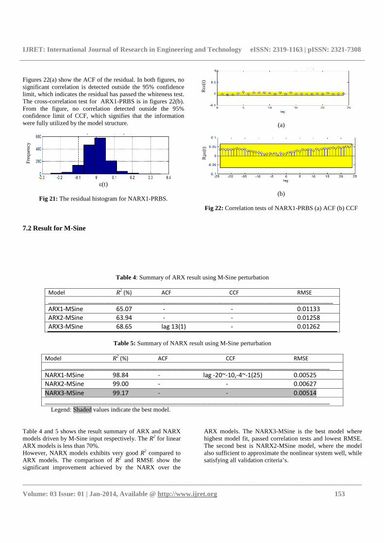
Figures 22(a) show the ACF of the residual. In both figures, no significant correlation is detected outside the 95% confidence limit, which indicates the residual has passed the whiteness test. The cross-correlation test for ARX1-PRBS is in figures 22(b). From the figure, no correlation detected outside the 95% confidence limit of CCF, which signifies that the information were fully utilized by the model structure.

ε(t)

Fig 21: The residual histogram for NARX1-PRBS.

7.2 Result for M-Sine

(a)

(b)

Fig 22: Correlation tests of NARX1-PRBS (a) ACF (b) CCF

Table 4: Summary of ARX result using M-Sine perturbation

Model R2 (%) ACF CCF RMSE

___________________________________________________________________________________________

ARX1-MSine 65.07 - - 0.01133

ARX2-MSine 63.94 - - 0.01258

ARX3-MSine 68.65 lag 13(1) - 0.01262

Table 5: Summary of NARX result using M-Sine perturbation

Model R2

(%) ACF CCF RMSE

___________________________________________________________________________________________

NARX1-MSine 98.84 - lag -20~-10,-4~-1(25) 0.00525

NARX2-MSine 99.00 - - 0.00627

NARX3-MSine 99.17 - - 0.00514

___________________________________________________________________________________________

Legend: Shaded values indicate the best model.

Table 4 and 5 shows the result summary of ARX and NARX models driven by M-Sine input respectively. The R2 for linear ARX models is less than 70%. However, NARX models exhibits very good R2 compared to ARX models. The comparison of R2 and RMSE show the significant improvement achieved by the NARX over the

ARX models. The NARX3-MSine is the best model where highest model fit, passed correlation tests and lowest RMSE. The second best is NARX2-MSine model, where the model also sufficient to approximate the nonlinear system well, while satisfying all validation criteria’s.

Rεε

(t)

R

µε(t

)

Fre

que

ncy


__________________________________________________________________________________________


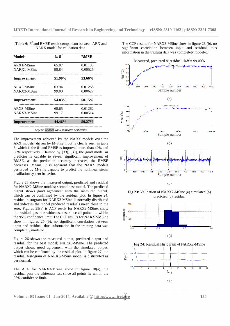
Table 6: R2 and RMSE result comparison between ARX and NARX model for validation data.

____________________________________________ Models % R2 RMSE ____________________________________________ ARX1-MSine 65.07 0.01133 NARX1-MSine 98.84 0.00525

------------------------------------------------------------------ Improvement 51.90% 53.66%

------------------------------------------------------------------ ARX2-MSine 63.94 0.01258 NARX2-MSine 99.00 0.00627

------------------------------------------------------------------ Improvement 54.83% 50.15%

------------------------------------------------------------------ ARX3-MSine 68.65 0.01262 NARX3-MSine 99.17 0.00514

------------------------------------------------------------------ Improvement 44.46% 59.27%

------------------------------------------------------------------ Legend: Shaded value indicates best result.

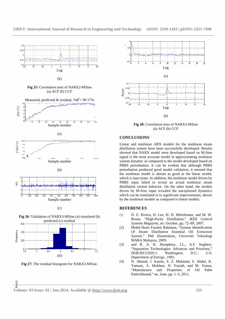
The improvement achieved by the NARX models over the ARX models driven by M-Sine input is clearly seen in table 6, which is the R2 and RMSE is improved more than 40% and 50% respectively. Claimed by [33], [39], the good model or predictor is capable to reveal significant improvement of RMSE, as the prediction accuracy increases, the RMSE decreases. Means, it is apparent that the NARX models perturbed by M-Sine capable to predict the nonlinear steam distillation system behavior. Figure 23 shows the measured output, predicted and residual for NARX2-MSine models; second best model. The predicted output shows good agreement with the measured output, which can be confirmed by the residual plot. In figure 24, residual histogram for NARX2-MSine is normally distributed and indicates the model produced residuals mean close to the zero. Figures 25(a) is ACF result for NARX2-MSine, show the residual pass the whiteness test since all points lie within the 95% confidence limit. The CCF results for NARX2-MSine show in figures 25 (b), no significant correlation between input and residual, thus information in the training data was completely modeled. Figure 26 shows the measured output, predicted output and residual for the best model; NARX3-MSine. The predicted output shows good agreement with the simulated output, which can be confirmed by the residual plot. In figure 27, the residual histogram of NARX3-MSine model is distributed as per normal. The ACF for NARX3-MSine show in figure 28(a), the residual pass the whiteness test since all points lie within the 95% confidence limit.

The CCF results for NARX3-MSine show in figure 28 (b), no significant correlation between input and residual, thus information in the training data was completely modeled.

Measured, predicted & residual, %R2= 99.00%

Sample number

(a)

Sample number

(b)

Sample number

(c)

Fig 23: Validation of NARX2-MSine (a) simulated (b)

predicted (c) residual

ε(t)

Fig 24: Residual Histogram of NARX2-MSine

Lag

(a)

y-ha

t (˚C

)

ε(t)

Rµε

(t)

ȳ(t

) (˚

C)

Rεε

(t)

Fre

que

ncy


__________________________________________________________________________________________


Lag

(b)

Fig 25: Correlation tests of NARX2-MSine

(a) ACF (b) CCF

Measured, predicted & residual, %R2= 99.17%

Sample number

(a)

Sample number

(b)

Sample number

(c)

Fig 26: Validation of NARX3-MSine (a) simulated (b)

predicted (c) residual

ε(t)

Fig 27: The residual histogram for NARX3-MSine.

Lag

(a)

Lag

(b)

Fig 28: Correlation tests of NARX3-MSine

(a) ACF (b) CCF CONCLUSIONS

Linear and nonlinear ARX models for the nonlinear steam distillation system have been successfully developed. Results showed that NARX model were developed based on M-Sine signal is the most accurate model in approximating nonlinear system dynamic as compared to the model developed based on PRBS perturbation. It can be evident that although PRBS perturbation produced good model validation, it seemed that the nonlinear model is almost as good as the linear model, which is inaccurate. In addition, the nonlinear model driven by PRBS input failed to reveal an actual nonlinear steam distillation system behavior. On the other hand, the models driven by M-Sine input revealed the unexplained dynamics which can be translated in to significant improvements, shown by the nonlinear models as compared to linear models. REFERENCES

[1] D. E. Rivera, H. Lee, H. D. Mittelmann, and M. W. Braun, “High-Purity Distillation,” IEEE Control Systems Magazine, no. October, pp. 72–89, 2007.

[2] Mohd Hezri Fazalul Rahiman, “System Identification Of Steam Distillation Essential Oil Extraction System.” Phd Dissertation, Universiti Teknologi MARA Malaysia, 2009.

[3] and R. A. K. Humphrey, J.L., A.F. Segibert, “Separation Technologies: Advances and Priorities,” DOE/ID/12920-1. Washington, D.C.: U.S. Department of Energy., 1991.

[4] N. Ahmad, J. Kasim, S. Z. Mahmud, S. Abdul, K. Yamani, A. Mokhtar, N. Yuziah, and M. Yunus, “Manufacture and Properties of Oil Palm Particleboard,” no. June, pp. 1–3, 2011.

y-ha

t (˚C

)

Rµ ε

(t)

Rεε

(t)

F

req

uen

cy

ȳ(t

) (˚

C)

ε(t)


__________________________________________________________________________________________


[5] M. L. L. W.L.Luyben, “Essential of Process Control,” Singapore;McGraw-Hills, 1997.

[6] A. A. Bachnas, “Linear Parameter-Varying Modeling of a High-Purity Distillation Collumn,” Master Science dissertation, no. System And Control At Delft University Of Technology, 2012.

[7] A. S. . Soni, “CONTROL-RELEVANT SYSTEM IDENTIFICATION USING NONLINEAR VOLTERRA AND VOLTERRA-LAGUERRE MODELS,” PhD Thesis, University of Pittsburgh , Submitted to the Graduate Faculty of the Science, 2006.

[8] Alina-Simona Baiesu, “Modeling a Nonlinear Binary Distillation Column,” CEAI, vol. 13, no. 1, pp. 49–53, 2011.

[9] N. Ismail, N. Tajjudin, M. Hezri, F. Rahiman, M. N. Taib, and U. T. Mara, “Modeling of Dynamic Response of Essential Oil Extraction Process,” pp. 298–301, 2009.

[10] M. H. A. Jalil, Z. Yusuf, N. N. Nordin, N. Kasuan, M. N. Taib, M. H. Fazalul, and U. T. Mara, “A Simulation Study of Model Reference Adaptive Control on Temperature Control of Glycerin Bleaching Process,” pp. 8–10, 2013.

[11] Z. Muhammad, Z. M. Yusoff, M. H. F. Rahiman, and M. N. Taib, “Steam temperature control for steam distillation pot using model predictive control,” IEEE 8th International Colloquium on Signal Processing and its Applications, pp. 474–479, Mar. 2012.

[12] J. Paduart, L. Lauwers, J. Swevers, K. Smolders, J. Schoukens, and R. Pintelon, “Identification of nonlinear systems using Polynomial Nonlinear State Space models,” Automatica, vol. 46, no. 4, pp. 647–656, Apr. 2010.

[13] Ir. Johan Paduart, “Identification of nonlinear systems using Polynomial Nonlinear State Space models,” Doctor of Engineering, Vrije Universiteit Brussel., 2010.

[14] Oliver Nelles, “Nonlinear System Identification, From Classical Approaches To Neural Networks and Fuzzy Models.” Springer Verlag, Heidelberg, Germany, 2000.

[15] L. Ljung, System Identification Theory for User. 2nd Edition,Prentice Hall, 1999.

[16] L. Ljung, “Perspectives on system identification,” Annual Reviews in Control, vol. 34, no. 1, pp. 1–12, Apr. 2010.

[17] L. Hyunjin, “A Plant-Friendly Multivariable System Identification Framework Based on Identification Test Monitoring,” PhD Dissertation, Arizona State University USA, no. December, 2006.

[18] M. H. F. Rahiman, M. N. Taib, R. Adnan, and Y. M. Salleh, “Analysis of weight decay regularisation in NNARX nonlinear identification,” 2009 5th International Colloquium on Signal Processing & Its Applications, pp. 355–361, Mar. 2009.

[19] I. Yunan, I. M. Yassin, S. Farid, S. Adnan, M. Hezri, and F. Rahiman, “Identification of Essential Oil Extraction System using Radial Basis Function ( RBF ) Neural Network,” IEEE 8th International Colloquium on Signal Processing And its Application, pp. 495–499, 2012.

[20] F. Q. Elizabeth, K. Beauchard, F. Ammouri, and P. Rouchon, “Stability and asymptotic observers of binary distillation processes described by nonlinear convection / diffusion models,” 2012 American Control Conference, pp. 3352–3358, 2012.

[21] A. N.-R. C.Bordons, “Model Based predictive control of an olive oil mill,” Journal of food Engineering, vol. 84, pp. 1–11, 2008.

[22] F. J. D. I. R.K.Pearson, B.A.Ogunnaike, “Identification of Discrete Convolution Models For Nonlinear Process,” IEEE Trans.,Acous.,Speech and Signal Processing, 1995.

[23] K. R. Thompson, “Implementation of Gaussian Process models for Nonlinear System Identification,” PhD Dissertation, Glasgow University, 2009.

[24] E. Martin, Linear Models of Nonlinear Systems, Linkoping., no. 985. Department of Electrical Engineering, Linkoping University, Sweden, 2005.

[25] K. Godfrey, “Perturbation Signals For System Identification.” Prentice Hall Internation (UK) Limited Hertfordshire UK, 2000.

[26] M. W. Braun, D. E. Rivera, A. Stenman, W. Foslien, and C. Hrenya, “Identification of a RTP Wafer Reactor Multi-level Pseudo-Random Signal Design and ‘ Model-on-Demand ’ Estimation Applied to Nonlinear Identification of a RTP Wafer Reactor,” LiTH-ISH-R-2156, ACC’99, San Diego, 1999.

[27] M. Deflorian and S. Zaglauer, “Design of Experiments for nonlinear dynamic system identification,” The 18th IFAC Congress Milano (Italy), pp. 13179–13184, 2011.

[28] N. Patcharaprakiti, K. Kirtikara, D. Chenvidhya, V. Monyakul, and B. Muenpinij, “Modeling of Single Phase Inverter of Photovoltaic System Using System Identification,” 2010 Second International Conference on Computer and Network Technology, pp. 462–466, 2010.

[29] T. Hatanaka, K. Uosaki, and M. Kogat, “Block Oriented Nonlinear Model Identification by Evolutionary Computation Approach.”

[30] G. Z. Ioan D.Landau, Digital Control Systems. Springer-Verlag London Limited, 2005.

[31] N. F. H. D.C.Montgomery, G.C. Runger, “Engineering Statistics,” 3rd.Edition, John Wiley & Sons, 2004.

[32] H.Demuth, “Neural Network Tollbox User Guides,” 4th.Edition Natick,USA, 2005.

[33] J.Sjoberg, “Non-linear Systen Identification with Neural Networks,” Ph.D Dissertation, Linkoping University, Linkoping, Sweden, 1995.


__________________________________________________________________________________________


[34] M.J.Roberts, “Signals ans systems: Analysis using transform methods and MATLAB,” 1st. edition New York; McGraw-Hill, 2013.

[35] L. K. H. Magnus Noorgard, O.Ravn, N.K.Poulsen, “Neural Network for modeling and control of dyanamics system,” London: Springer-Verlag London Ltd, 2000.

[36] M. I. Natick, MA, “Curve Fitting Toolbox User’s Guide, Release 2007a,” 2007.

[37] A. B. D.Kundu, “Statisticl Computing -Existing Methods And Recent Developments,” Harrow; U.K, Alpha Science Internation Ltd., 2004.

[38] C. C. J.K. Taylor, “Statistical technologies for Data Analysis,” 2nd Edition, Florida,U.S.A: Chapman and Hall/CRC, 2004.

[39] M. H. H.Demuth, M.Beale, “Neural Network Toolbox User’s Guide.” 2005.

system identification of a steam distillation pilotscale

Documents