system model representationfaculty.uml.edu/pavitabile/22.451/dynamic_systems_system... · system...
TRANSCRIPT

1 Dr. Peter AvitabileModal Analysis & Controls Laboratory22.451 Dynamic Systems – System Representation
System Model Representation
Peter AvitabileMechanical Engineering DepartmentUniversity of Massachusetts Lowell

2 Dr. Peter AvitabileModal Analysis & Controls Laboratory22.451 Dynamic Systems – System Representation
System Model Representation
System models can be developed in a variety of forms. Once the governing equations are developed, then the system characteristics and response can be determined.
Consider a simple mechanical system subjected to initial conditions
and oo xx & m
c
k
x(t)
f(t)

3 Dr. Peter AvitabileModal Analysis & Controls Laboratory22.451 Dynamic Systems – System Representation
System Model Representation
The governing differential equation (chap 4) describing the motion is
Note that there is only one generalized coordinate to describe the motion – x
00 x)0(x;x)0(x && ==0kxxcxm =++ &&& with
Note if a force is applied instead of an initial condition, there is still only one generalized equation
)t(fkxxcxm =++ &&&

4 Dr. Peter AvitabileModal Analysis & Controls Laboratory22.451 Dynamic Systems – System Representation
State-Space Representation
Another approach commonly used is to represent the system as a larger system of equations – The second order ODE with two variables to describe the “state” of the system rather than one variable
The number of state variable depends on the number of possible initial conditions
For the 2nd order ODE
00 x&xIC)t(fkxxcxm &&&& =++
has two state variables –displacement and velocity

5 Dr. Peter AvitabileModal Analysis & Controls Laboratory22.451 Dynamic Systems – System Representation
Example
00 x&xIC)t(fkxxcxm &&&& =++
The system is described by
The two mutual conditions of are required to completely describe the “state” of the system. Hence there are two state variables.
00 & xx &
m
c
k
x(t)
f(t)

6 Dr. Peter AvitabileModal Analysis & Controls Laboratory22.451 Dynamic Systems – System Representation
Example – State Space
In order to solve this, there are three mutual conditions required namely )0(x),0(x),0(x 121 &
Assume 0xxxx 2111 =−++ &&&
0xx2x 212 =++&

7 Dr. Peter AvitabileModal Analysis & Controls Laboratory22.451 Dynamic Systems – System Representation
State Space – General Formulation
State-variable equations
Where x is a state variableu is an inputf is some function
)t;u...u;x...,x(fx m1n122 =&
)t;u...u;x...,x(fx m1n111 =&
)t;u...u;x...,x(fx m1n1nn =&M

8 Dr. Peter AvitabileModal Analysis & Controls Laboratory22.451 Dynamic Systems – System Representation
System Outputs
State variables can be expressed as
System variables can be expressed as
)t;u...u;x...,x(hy m1n12 =
)t;u...u;x...,x(hy m1n11 =
M
Note that f and h can be general nonlinear functions
)t,u,x(fx =&
)t,u,x(hy =
State Space – General Formulation

9 Dr. Peter AvitabileModal Analysis & Controls Laboratory22.451 Dynamic Systems – System Representation
For a linear system, this simplifies to
Linear State Variable
mm1111nn11n1 ub...ubxa...xax ++++=&
M
mm2121nn21212 ub...ubxa...xax ++++=&
mnm11nnnn11nn ub...ubxa...xax ++++=&
Linear Outputs
mm1111nn11111 ud...udxc...xcy +++++=
Mmm2121nn21212 ud...udxc...xcy +++++=
mpm11pnpn11pn ud...udxc...xcy +++++=
State Space – General Formulation

10 Dr. Peter AvitabileModal Analysis & Controls Laboratory22.451 Dynamic Systems – System Representation
=
n
2
1
x
xx
xM
State Vector Input VectorOutput Vector
=
p
2
1
y
yy
yM
=
m
2
1
u
uu
uM
State Space – General Formulation

11 Dr. Peter AvitabileModal Analysis & Controls Laboratory22.451 Dynamic Systems – System Representation
→
↓→
↓=
nn1n
n111
aa
aaA
State Matrix
Output Matrix
Input Matrix
Transmission Matrix
→
↓→
↓=
mm1m
m111
bb
bbB
→
↓→
↓=
nn1n
n111
cc
ccC
→
→↓=
mm1m
m111
dd
ddD
State Equation
Output Equation
{ } [ ]{ } [ ]{ }uBxAx +=&
{ } [ ]{ } [ ]{ }uDxCy +=
State Space – General Formulation

12 Dr. Peter AvitabileModal Analysis & Controls Laboratory22.451 Dynamic Systems – System Representation
Example – State Space
Governing Equation
)t(fkxxcxm =++ &&&
The state variables are
In order to rewrite the governing equation as 2 first order ODE, the following relationship exists
xx&xx 21 &==
21 xx =&
m
c
k
x(t)
f(t)

13 Dr. Peter AvitabileModal Analysis & Controls Laboratory22.451 Dynamic Systems – System Representation
Substituting into the governing equation21 xx =&
)t(fkxcxxm 122 =++&
[ ])t(fkxcxm1x 122 +−−=&
which is
Now the state variables equations are:
[ ])t(fkxcxm1x
xx
122
21
+−−=
=
&
&
Example – State Space

14 Dr. Peter AvitabileModal Analysis & Controls Laboratory22.451 Dynamic Systems – System Representation
This can be written in matrix form as:
)t(f0
xx10
xx
m1
2
1
mc
mk
2
1
+
−−
=
&
&
[ ] u0xx
01y2
1 ⋅+
=
which is:
Example – State Space

15 Dr. Peter AvitabileModal Analysis & Controls Laboratory22.451 Dynamic Systems – System Representation
{ } [ ]{ } [ ]{ }uBxAx +=&
)t(f0
xx10
xx
m1
2
1
mc
mk
2
1
+
−−
=
&
&
{ } [ ]{ } [ ]{ }uDxCy +=
[ ] u0xx
01y2
1 ⋅+
=
Example – State Space

16 Dr. Peter AvitabileModal Analysis & Controls Laboratory22.451 Dynamic Systems – System Representation
Example – Electrical Circuit
Source: Dynamic Systems – Vu & Esfandiari

17 Dr. Peter AvitabileModal Analysis & Controls Laboratory22.451 Dynamic Systems – System Representation
Example – Electrical Circuit
Source: Dynamic Systems – Vu & Esfandiari

18 Dr. Peter AvitabileModal Analysis & Controls Laboratory22.451 Dynamic Systems – System Representation
Example – Electrical Circuit
Source: Dynamic Systems – Vu & Esfandiari

19 Dr. Peter AvitabileModal Analysis & Controls Laboratory22.451 Dynamic Systems – System Representation
Input-Output EquationsAnother common form is the input-output equation. A single Diff Eq with time derivatives
( ) ( ) yaya...yay n1n1n
1n ++++ −
− &
( ) ( ) ubub...ubub m1m1m
1m
0 ++++= −− &
Note: y(n) is the nth derivativea and b are constant coefficientsy is system outputu is system input
These equations are normally cumbersome and a Laplace Transform is used resulting in a set of algebraic equations.

20 Dr. Peter AvitabileModal Analysis & Controls Laboratory22.451 Dynamic Systems – System Representation
Example – I/O Equation
Source: Dynamic Systems – Vu & Esfandiari

21 Dr. Peter AvitabileModal Analysis & Controls Laboratory22.451 Dynamic Systems – System Representation
Example – I/O Equation
Source: Dynamic Systems – Vu & Esfandiari

22 Dr. Peter AvitabileModal Analysis & Controls Laboratory22.451 Dynamic Systems – System Representation
System Transfer FunctionOnce again, consider the linear time-invariant differential equation as:
( ) ( ) yaya...yay n1n1n
1n ++++ −
− &
( ) ( ) ubub...ubub m1m1m
1m
0 ++++= −− &
Assuming the initial conditions are zero, the Laplace Transform yields:
( ) )s(yasa...sas n1n1n
1n ++++ −
−
( ) )s(Ubsb...sbsb m1m1m
1m
0 ++++= −−

23 Dr. Peter AvitabileModal Analysis & Controls Laboratory22.451 Dynamic Systems – System Representation
System Transfer Function
So that the system transfer function is
n1n1n
1n
m1m1m
1m
0
asa...sasbsb...sbsb
)s(U)s(Y)s(G
++++++++
==−
−−
−
This is the system transfer function for a single input-single output (SISO). If there are other inputs and outputs to consider, then the problem becomes a multiple input-multiple output (MIMO)

24 Dr. Peter AvitabileModal Analysis & Controls Laboratory22.451 Dynamic Systems – System Representation
Relationship between state space and system transfer function
State space
Transfer function
DuCxyBuAxx
+=+=&
)s(U)s(Y)s(G =
Laplace Transform of State equation (w/IC = 0) )s(DU)s(CX)s(Y
)s(BU)s(AX)s(sX+=+=
( ))s(DU)s(CX)s(Y)s(BU)s(XAsI
+==−
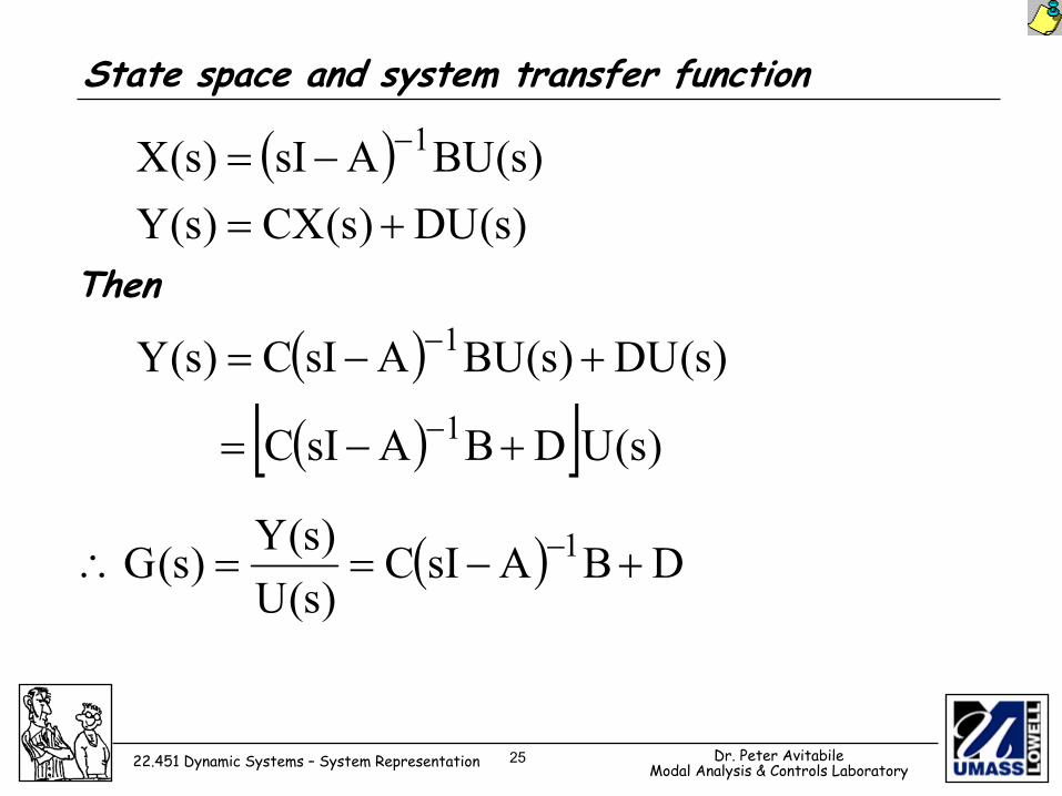
25 Dr. Peter AvitabileModal Analysis & Controls Laboratory22.451 Dynamic Systems – System Representation
State space and system transfer function
( ))s(DU)s(CX)s(Y)s(BUAsI)s(X 1
+=−= −
Then
( ) )s(DU)s(BUAsIC)s(Y 1 +−= −
( )[ ] )s(UDBAsIC 1 +−= −
( ) DBAsIC)s(U)s(Y)s(G 1 +−==∴ −

26 Dr. Peter AvitabileModal Analysis & Controls Laboratory22.451 Dynamic Systems – System Representation
State space and system transfer function
Realizing that ( ) ( )( )AsIdet
AsIadjAsI 1
−−
⇒− −
So that( )( ) D
AsIdetBAsICadj)s(G +
−−
=

27 Dr. Peter AvitabileModal Analysis & Controls Laboratory22.451 Dynamic Systems – System Representation
Example – State Space Representation
The SDOF state equation:DuCxyBuAxx
+=+=&
=
−−
=
=
m1
mc
mk
2
1
0B
10A
xx
x
[ ]
0D
01C
)t(fu
=
=
=

28 Dr. Peter AvitabileModal Analysis & Controls Laboratory22.451 Dynamic Systems – System Representation
Now
( )
+−
=−mc
mk s
1sAsI
( ) ( )
+−
++=− −
mc
mk
mk
mc
1s1s
ss1AsI
Then
[ ] ( )
+−
++=
m1
mc
mk
mk
mc
0s1s
ss101)s(G
( ) [ ] ( )( )
+++=
mc
m1
m1
mk
mc s
01ss1
Example – State Space Representation

29 Dr. Peter AvitabileModal Analysis & Controls Laboratory22.451 Dynamic Systems – System Representation
which is the system transfer function. State space representation can also be obtained from the input-output equation.
kcsms1)s(G 2 ++
=⇒
( ) m1
ss1
mk
mc ⋅++
=
Example – State Space Representation

30 Dr. Peter AvitabileModal Analysis & Controls Laboratory22.451 Dynamic Systems – System Representation
LinearizationMany times the equations describing a system may be non-linear. Often, these equations can be “linearized” to determine an acceptable solution. The basic approach is to perform a Taylor Series Expansion about some “operating” point to find an equivalent linear set of equations with the assumption that the system will operate around this point.

31 Dr. Peter AvitabileModal Analysis & Controls Laboratory22.451 Dynamic Systems – System Representation
Graphical InterpretationThe function can be evaluated in the vicinity of and causes to result.
Considering a small variation of ∆x results in ∆f. In this region, the slope is approximated
by
x f
xxdxdfm ==
Thus xmf)xx(mff ∆=∆⇒−=−

32 Dr. Peter AvitabileModal Analysis & Controls Laboratory22.451 Dynamic Systems – System Representation
Taylor Series ExpansionThe analytical counterpart to the graphical representation is performed.The Taylor Series Expansion about the pointfor a non-linear function
x)x(f
K+−′′+−′+= ==2
xxxx )xx()x(f!21)xx()x(f)x(f)x(f
In the event that is small then higher order terms can be negligible. Thus
)xx( −
)xx()x(f)x(f)x(f xx −′+≈ =
x)x(fyy xx ∆′+≈ =
OR as done graphically:

33 Dr. Peter AvitabileModal Analysis & Controls Laboratory22.451 Dynamic Systems – System Representation
Example - Linearization
Source: Dynamic Systems – Vu & Esfandiari

34 Dr. Peter AvitabileModal Analysis & Controls Laboratory22.451 Dynamic Systems – System Representation
Example - Linearization
Source: Dynamic Systems – Vu & Esfandiari

35 Dr. Peter AvitabileModal Analysis & Controls Laboratory22.451 Dynamic Systems – System Representation
Mount Stiffness
Example
Car Suspension

36 Dr. Peter AvitabileModal Analysis & Controls Laboratory22.451 Dynamic Systems – System Representation
Example – Nonlinear Spring
Source: Dynamic Systems – Vu & Esfandiari

37 Dr. Peter AvitabileModal Analysis & Controls Laboratory22.451 Dynamic Systems – System Representation
Example – Nonlinear Spring
Source: Dynamic Systems – Vu & Esfandiari

38 Dr. Peter AvitabileModal Analysis & Controls Laboratory22.451 Dynamic Systems – System Representation
Example – Nonlinear Spring
Source: Dynamic Systems – Vu & Esfandiari

39 Dr. Peter AvitabileModal Analysis & Controls Laboratory22.451 Dynamic Systems – System Representation
Example – Nonlinear Spring
Source: Dynamic Systems – Vu & Esfandiari

40 Dr. Peter AvitabileModal Analysis & Controls Laboratory22.451 Dynamic Systems – System Representation
Example – Nonlinear Spring
Source: Dynamic Systems – Vu & Esfandiari

41 Dr. Peter AvitabileModal Analysis & Controls Laboratory22.451 Dynamic Systems – System Representation
Example – Nonlinear Spring
Source: Dynamic Systems – Vu & Esfandiari