System of Linear Equations

Nattee Niparnan

LINEAR EQUATIONS

Linear Equation

• An Equation– Represent a straight line– Is a “linear equation” in the variable x and y.

• General form– ai a real number that is a coefficient of xi

– b another number called a constant term

System of a Linear Equation

• A collection of several linear equations– In the same variables

• What about– A linear equation• in the variables x1, x2 and x3

– Another equation• in the variables x1, x2,x3 and x4

– Do they form a system of linear equation?

Solution

• A linear equation

• Has a solution

• When

• It is called a solution to the system if it is a solution to all equations in the system

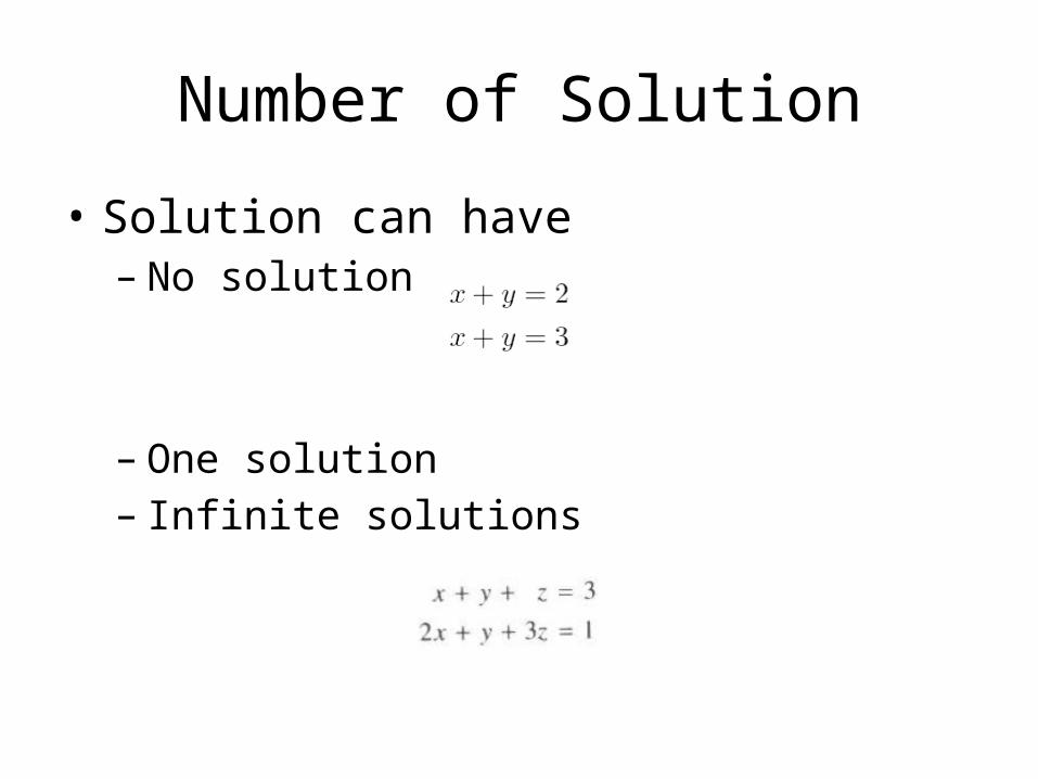
Number of Solution

• Solution can have– No solution

– One solution– Infinite solutions

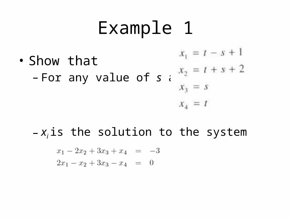
Example 1

• Show that– For any value of s and t

– xi is the solution to the system

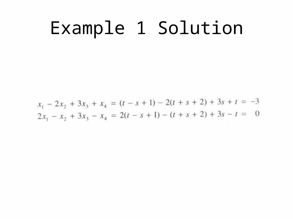
Example 1 Solution

Parametric Form

• Solution of the system in Equation 1 is described in a parametric form– It is given as a function in parameters s and t– It is called a general solution of the system

• Every linear equation system having solutions– Can be written in parametric form

Try another one

• Solve it using parametric form

• In term of x and z

• In term of y and z

There are several general

solutions

Geometrical Point of View

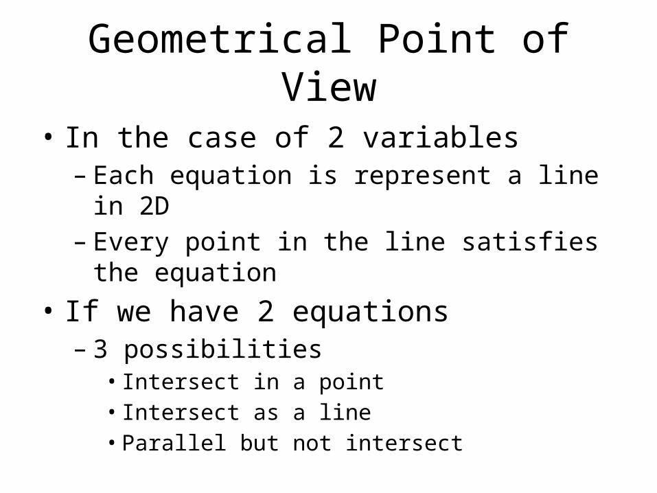
• In the case of 2 variables– Each equation is represent a line in 2D– Every point in the line satisfies the equation

• If we have 2 equations– 3 possibilities• Intersect in a point• Intersect as a line• Parallel but not intersect

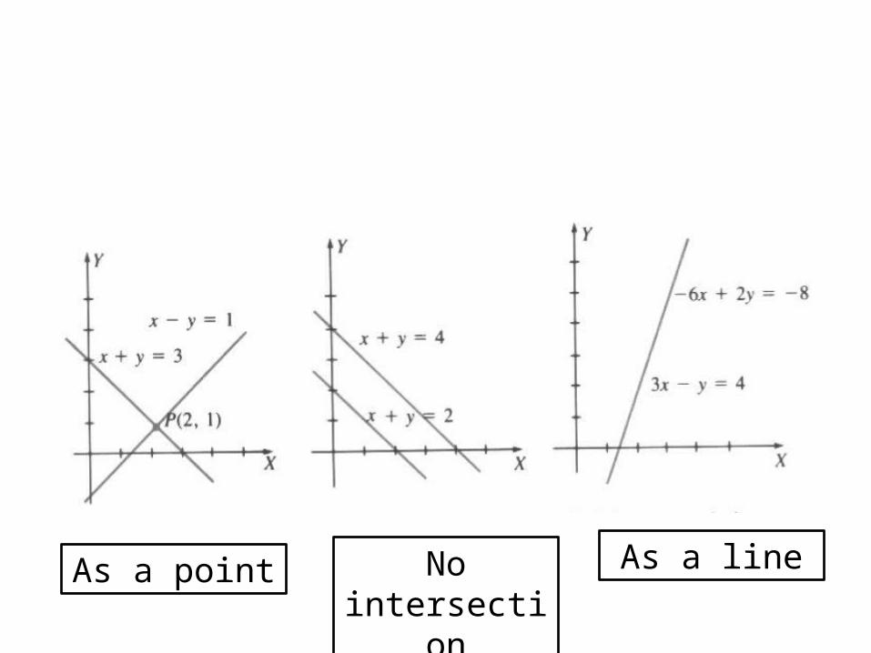
As a point No intersection

As a line

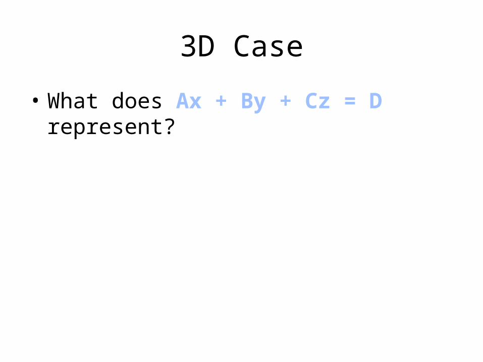
3D Case

• What does Ax + By + Cz = D represent?

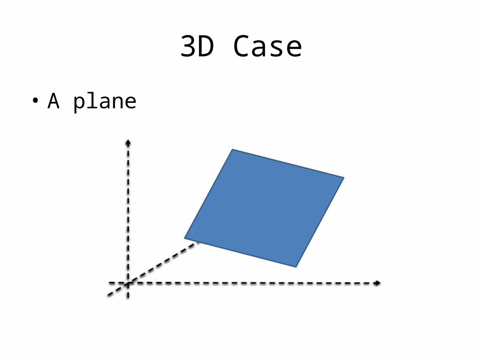
3D Case

• A plane

Higher Space?

• Somewhat difficult to imagine– But Linear Algebra will, at least, provides some

characteristic for us

Cogito, ergo sum

I also speak Calculus

MANIPULATING THE SYSTEM

Augmented Matrix

Augmented matrix

Coefficient matrix

Constantmatrix

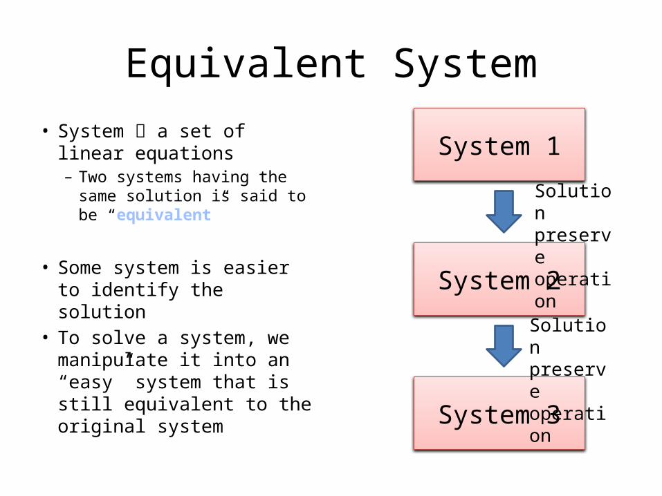
Equivalent System

• System a set of linear equations– Two systems having the same

solution is said to be “equivalent”

• Some system is easier to identify the solution

• To solve a system, we manipulate it into an “easy” system that is still equivalent to the original system

System 1

System 2

System 3

Solution preserve operation

Solution preserve operation

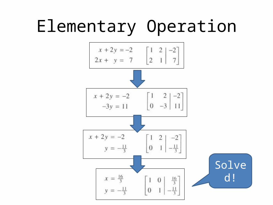
Elementary Operation

Solved!

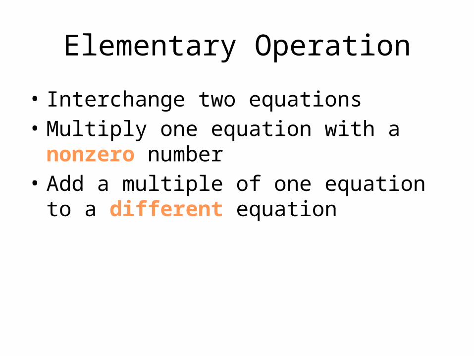
Elementary Operation

• Interchange two equations• Multiply one equation with a nonzero number• Add a multiple of one equation to a different

equation

Theorem 1

• Suppose that an elementary operation is performed on a linear equation system– Then, there solution are still the same

Proof

Elementary Row Operation

• We don’t really do the elementary operation• We write the system as an augmented matrix

and then perform “elementary row operation” on that matrix

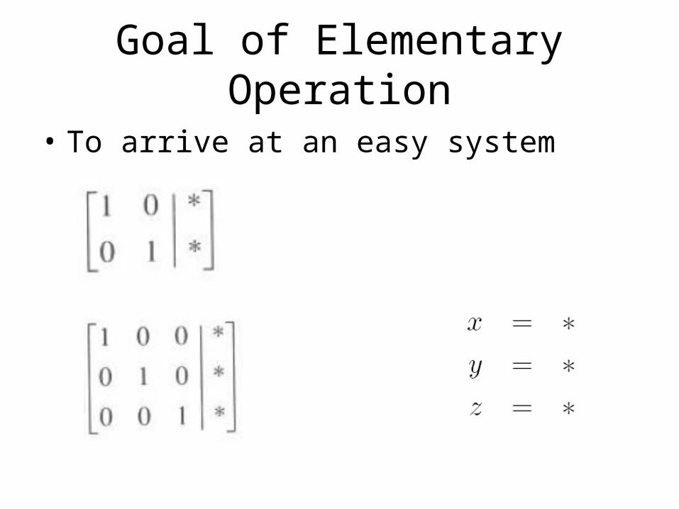
Goal of Elementary Operation

• To arrive at an easy system

GAUSSIAN ELIMINATION

Gaussian Elimination

• An algorithm that manipulate an augmented matrix into a “nice” augmented matrix

Row Echelon Form

• A matrix is in “Row Echelon Form” (called row echelon matrix) if– All zero rows are at the bottom– The first nonzero entry from the left in each

nonzero row is 1 • (that 1 is called a leading 1 of that row)

– Each leading 1 is to the right of all leading 1’s in the row above it

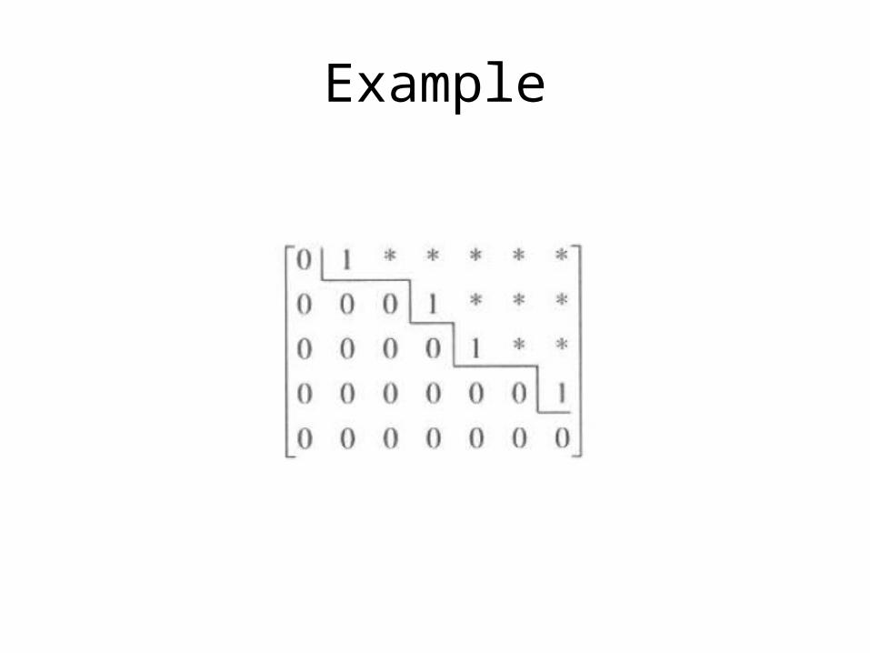
Example

Echelon?

• Diagonal Formation

Reduced Row Echelon

• The leading 1 is the only nonzero element in that column

row echelon

Reduced row echelon

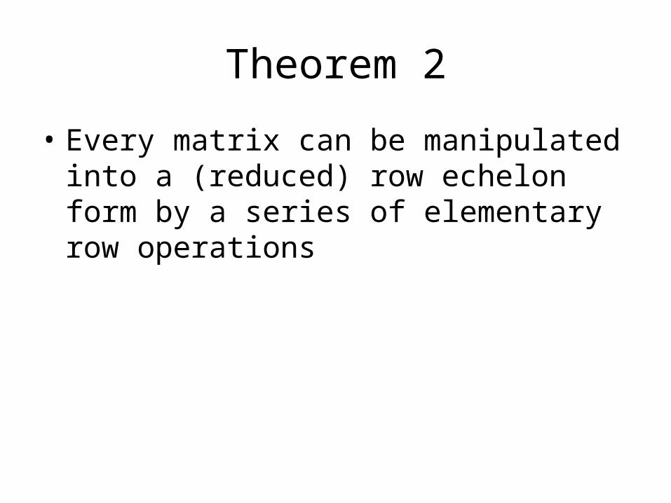
Theorem 2

• Every matrix can be manipulated into a (reduced) row echelon form by a series of elementary row operations

Using (Reduced) Row Echelon Form

Using (Reduced) Row Echelon Form

No solution

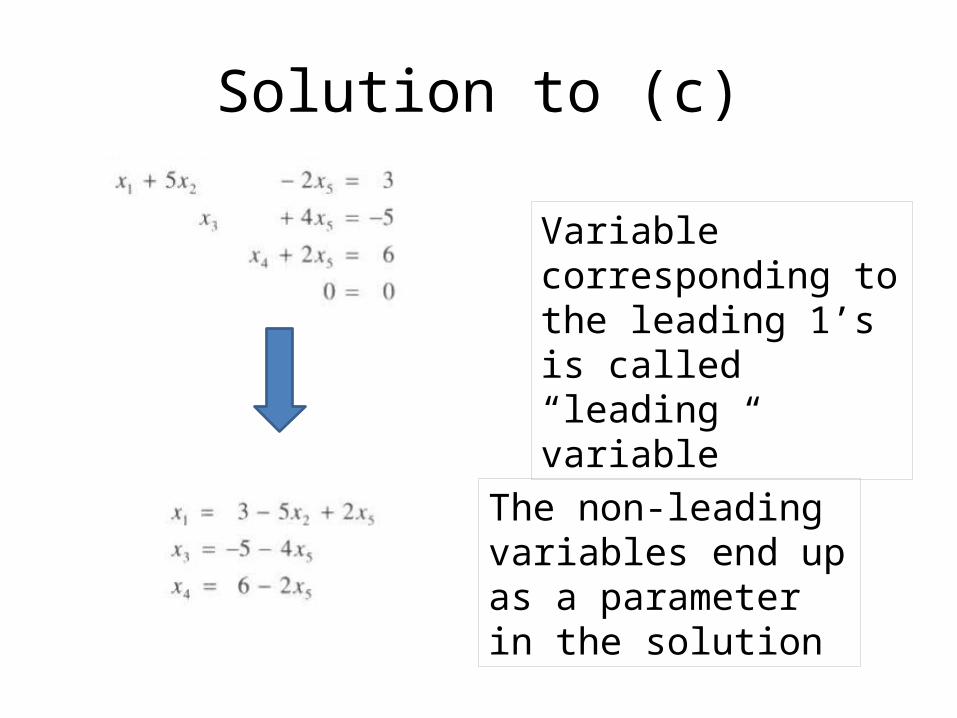
Solution to (c)

Variable corresponding to the leading 1’s is called “leading variable”

The non-leading variables end up as a parameter in the solution

Gaussian Elimination

• If the matrix is all zeroes stop• Find the first column from the left containing a

non zero entry (called it A) and move the row having that entry to the top row

• Multiply that row by 1/A to create a leading 1• Subtract multiples of that row from rows below

it, making entry in that column to become zero• Repeat the same step from the matrix consists of

remaining row

Gauss?

Redundancy

Subtract 2 time row 1 from row 2AndSubtract 7 time row 1 from row 3

Subtract 2 time row 2 from row 1AndSubtract 3 time row 2 from row 3

Redundancy

redundancy

Observe that the last row is the triple of the second row

Back Substitution

• Gaussian Elimination brings the matrix into a row echelon form– To create a reduced row echelon form• We need to change step 4 such that it also create zero

on the “above” row as well• Usually, that is less efficient

• It is better to start from the row echelon form and then use the leading 1 of the bottom-most row to create zero

Example

Example

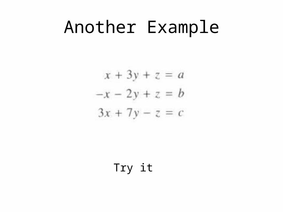
Another Example

Try it

Solution

Must be 0

Rank

• It is (later) shown that, for any matrix A, it has the same “Reduced row echelon form”– Regardless of the elementary row operation performed

• But it s not true for “row echelon form”– Different sequence of operations leads to different row

echelon matrix• However, the number of leading 1’s is always the same

– Will be proved later• Hence, the number of leading 1’s depends on A• The number of leading 1’s is called rank of A

Theorem 3

• Suppose a system of m equation on n variables has a solution, if the rank of the augmented matrix is r – the set of the solution involve exactly n-r

parameters

Homogeneous Equation

When b = 0What is the solution?

Homogeneous Linear System

• Xi = 0 is always a solution to the homogeneous system– It is called “trivial” solution

• Any solution having nonzero term is called “nontrivial” solution

Existence of Nontrivial Solution to the homogeneous system

• If it has non-leading entry in the row echelon form– The solution can be described as a parameter

• Then it has nonzero solution!!!– Nontrivial

• When will we have non-leading entry?– When we have more variable than equation

GEOMETRICAL VIEW OF LINEAR EQUATION

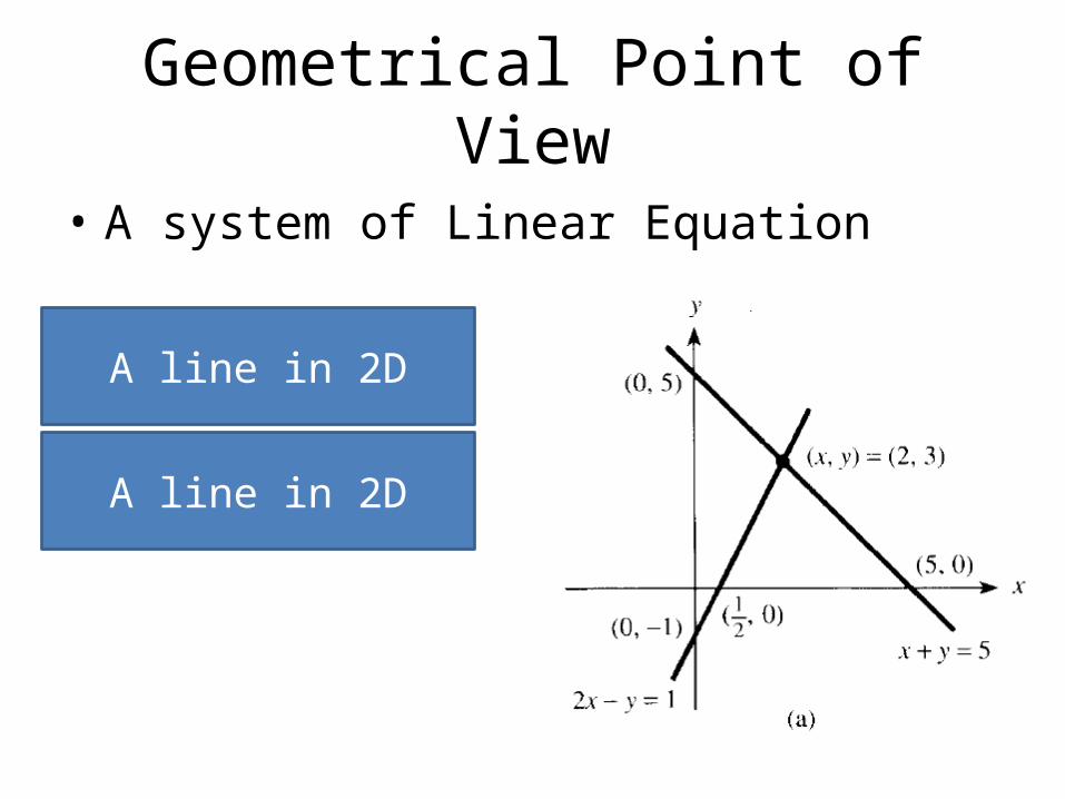
Geometrical Point of View

• A system of Linear Equation

A line in 2D

A line in 2D

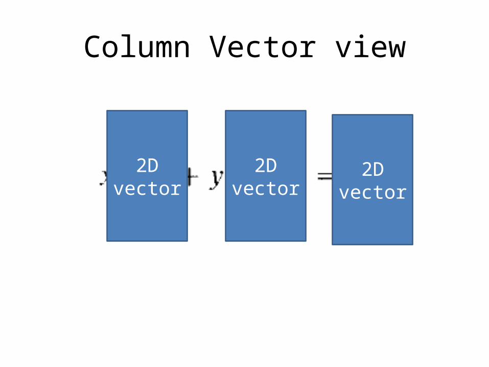
Column Vector view

2D vector

2D vector

2D vector

Network Flow Problem

• A graph of traffic– Node = intersection– Edge = road– Do we know the flow at each road?

Network Flow Problem

• Rules– For each node, traffic in equals traffic out

Formulate the System

• Five equations, six vars

Solve it