SERI/TR-253-2694UC Category: 62DE85016892

System Performance andCost SensitivityComparisons of StretchedMembrane HeliostatReflectors with CurrentGeneration Glass/MetalConcepts

L. M. MurphyJ. V. AndersonW. ShortT. Wendelln

December 1985

Prepared under Task No. 5111.31FTP No. 510

Solar Energy Research InstituteA Division of Midwest Research Institute

1617 Cole BoulevardGolden, Colorado 80401

Prepared for the

U.S. Department of EnergyContract No. DE-AC02-83CH10093

NOTICE

This report was prepared as an account of work sponsored by the United States Government. Neither theUnited States nor the United States Department of Energy, nor any of their employees, nor any of theircontractors, subcontractors, or their employees. makes any warranty, expressed or implied, or assumes anylegal liability or responsibility for the accuracy, completeness or usefulness of any information. apparatus,product or process disclosed, or represents that its use would not infringe privately owned rights.

Printed in the United States of AmericaAvailable from:

National Technical Information ServiceU.S. Department of Commerce

5285 Port Royal RoadSpringfielc;i, VA 22161

Price: Microfiche A01Printed Copy AD5

Cooes IHe used for pricing all publications. The code is determined by the number of pages in the publication.rntormauon pertainIng 10 the prrcing codes can be found in the current issue of the following publications,wrucn are generally available in most libraries: Energy Research Abstracts, (ERA): Government ReportsAnnounclJments and Index (GRA and I): Scientific and Tochnical Abstract Reports (STAR): and publication,NTIS-PR·360 available from NTIS at the above address.

TR-2694

PREFACE

The research and development described in this document was conducted withinthe u.s. Department of Energy's Solar Thermal Technology Program. The goal ofthis program is to advance the engineering and scientific understanding ofsolar thermal technology and to establish the technology base from whichprivate industry can develop solar thermal power production options forintroduction into the competitive energy market.

Solar thermal technology concentrates the solar flux using tracking mirrors orlenses onto a receiver where the solar energy is absorbed as heat andconverted into electricity or incorporated into products as process heat. Thetwo primary solar thermal technologies, central receivers and distributedreceivers, employ various point and line-focus optics to concentratesunlight. Current central receiver systems use fields of heliostats (two-axistracking mirrors) to focus the sun's radiant energy onto a single, tower­mounted receiver. Point focus concentrators up to 17 meters in diameter trackthe sun in two axes and use parabolic dish mirrors or Fresnel lenses to focusradiant energy onto a receiver. Troughs and bowls are line-focus trackingreflectors that concentrate sunlight onto receiver tubes along their focallines. Concentrating collector modules can be used alone or in a multimodulesystem. The concentrated radiant energy absorbed by the solar thermalreceiver is transported to the conversion process by a circulating workingfluid. Receiver temperatures range from lOOoC in low-temperature troughs toover 15000C in dish and central receiver systems.

The Solar Thermal Technology Program is directing efforts to advance andimprove each system concept through solar thermal materials, components, andsubsystems research and development and by testing and evaluation. Theseefforts are carried out with the technical direction of DOE and its network offield laboratories that works with private industry. Together they haveestablished a comprehensive, goal-directed program to improve performance andprovide technically proven options for eventual incorporation into theNation's energy supply.

To successfully contribute to an adequate energy supply at reasonable cost,solar thermal energy must be economically competitive with a variety of otherenergy sources. The Solar Thermal Program has developed component sandsystem-level performance targets as quantitative program goals. These targetsare used in planning research and development activities, measuring progress,assessing alternative technology options, and developing optimal components.These targets will be pursued vigorously to ensure a successful program.

This report presents work supported by the Division of Solar ThermalTechnology of the U.S. Department of Energy (DOE) as part of the Solar EnergyResearch Institute research effort on innovative concentrators. Research onstretched membrane heliostat modules has been emphasized as part of theinnovative concentrator effort for some time because of their potentialcost/performance benefits over the current technology for heliostats.However, the potential of stretched membrane heliostats from a systemsperspective over a wide range of design and operational parameters has notbeen studied until this time. The purpose of this report is to document and

iii

TR-2694

present the findings of a study comparing stretched membrane and glass/metalheliostats from a systems perspective. In this study, we have investigatedthe sensitivity of the relative performance and cost of fields of heliostatsto a fairly large number of parameter variations, including system size anddelivery temperature, along with heliostat module size, reflective surfacespeculari ty, hemispherical reflectance, and macroscopic surface qual i ty forboth focused and unfocused stretched membrane modules.

The authors would like to thank both Martin Scheve and Frank Wilkins of theU.S. Department of Energy for their support in this effort. The authors wouldalso like to note that this work builds upon an extensive information base onthe optical performance of solar concentrators that has been developed for theDOE Solar Thermal Program by the Sandia National Laboratories.

Engineer

Approved for

SOLAR ENERGY RESEARCH INSTITUTE

~ Q,Qlk:~P. Thornton, ManagerThermal Systems and Engineering Branch

L. J.Solar

annon, Directorat Research Division

iv

TR-2694

SUMMARY

In this report we compare stretched membrane heliostats with state-of-the-artglass/metal heliostats from a systems perspective. We have investigated thesensitivity of the relative performance and cost of fields of heliostats to alarge number of parameter variations, including system size, delivery tempera­ture, heliostat module size, surface specularity, hemispherical reflectance,and macroscopic surface quality for both focused and unfocused stretched mem­brane modules.

Effort in this project has been directed in two major areas:

• Assessing the performance of individual modules based on the findings ofcurrent structural analyses for stretched membrane modules, including thereview of existing assumptions and practices for analyzing heliostats

• Conducting systems sensitivity studies of fields of heliostats on whichthe parameter variations are performed.

The performance comparisons are based on the annual delivered energy. Thesystem designs are optimized for performance only. Cost sensitivities arebased on assumed costs for these performance optimized systems.

A major feature of this study is that it brings together into a unifiedpresentation a large number of results and definitions from systems, struc­tural, and optical materials investigations conducted for DOE by SandiaNational Laboratories (SNLL) and the Solar Energy Research Institute (SERl).

Gaamm KULES AHD MAJOR ASSUMPTIONS

Some of the ground rules and major assumptions used in this study are listedbelow.

Heliostats

• 100-m2 glass/metal heliostats were used as the baseline standard of com­parison AS in DeLaquil and Anderson [11]. Each heliostat has 12 mirrorpanels in a 2 x 6 ft array focused in 2 directions and canted on-axis.

• Both focused and unfocused stretched membrane heliostats usi~g the ~ouble

membr~ne construction were studied. They were sized at 25 m , 50 m , and100 m •

• The focused stretched membrane heliostats were assumed to use thevacuum/pressure active control of the reflector surface proposed by SNLL.

• All deformations in the unfocused stretched membrane heliostats were mea­sured relative to a perfectly flat reference plane.

• We have utilized standard documented approaches in considering reflectorsurface error effects. Specifically, in the analysis and the discussionswe assumed that specular reflectivity can be represented as the product

v

TR-2694

of two independent functions; i.e., the total hemispherical reflectivitytimes a geometric function of the cone angle containing the scatteredreflective beam. We considered independent variations in both the hemis­pherical reflectivity and the variance of the cone angle about the spec­ular directions. In addition, macroscopic surface quality effects causedby wind-, weight-, and manufacturing-induced errors are cons idered asreflected-beam broadening effects along with the microscopic specularityvariations about the specular direction.

Balance of System

• Only single cavity, open aperture receivers coupled to north fields wereconsidered.

• The study investigated IPH systems with delivery temperatures of 450°,750°, and 10500 e for pl/nt sizes of 7~ MWt h and 450 MWt h (field sizes ofapproximately 100,000 m and 700,000 m ).

• No storage was considered for any of the cases.

rIBDIBCS ABD COBCLUSIOBS

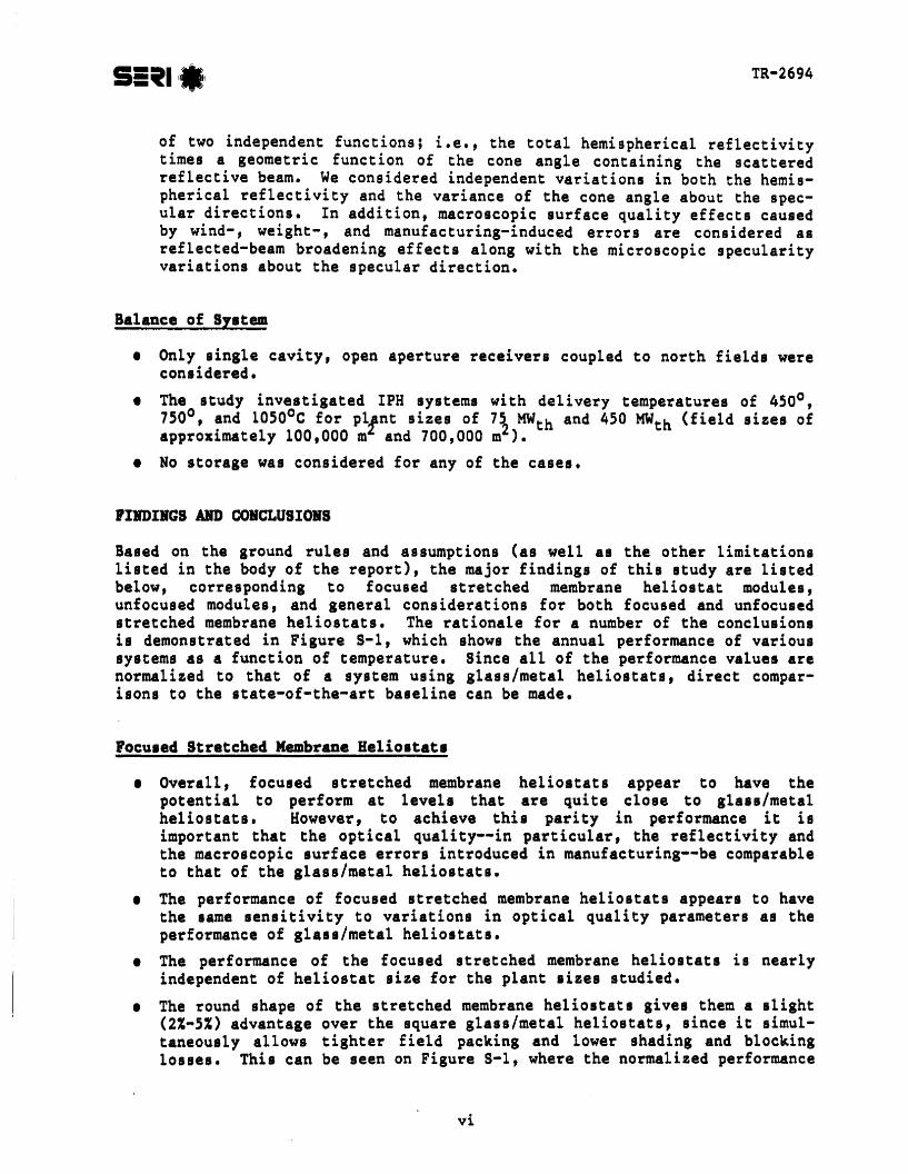
Based on the ground rules and assumptions (as well as the other limitationslisted in the body of the report), the major findings of this study are listedbelow, corresponding to focused stretched membrane heliostat modules,unfocused modules, and general considerations for both focused and unfocusedstretched membrane heliostats. The rationale for a number of the conclusionsis demonstrated in Figure 8-1, which shows the annual performance of varioussystems as a function of temperature. Since all of the performance values arenormalized to that of a system using glass/metal heliostats, direct compar­isons to the state-of-the-art baseline can be made.

rocused Stretched Membrane Heliostats

• Overall, focused stretched membrane heliostats appear to have thepotential to perform at levels that are quite close to glass/metalheliostats. However, to achieve this parity in performance it isimportant that the optical quality--in particular, the reflectivity andthe macroscopic surface errors introduced in manufacturing--be comparableto that of the glass/metal heliostats.

• The performance of focused stretched membrane heliostats appears to havethe same sensitivity to variations in optical quality parameters as theperformance of glass/metal heliostats.

• The performance of the focused stretched membrane heliostats is nearlyindependent of heliostat size for the plant sizes studied.

• The round shape of the stretched membrane heliostats gives them a slight(2%-5%) advantage over the square glass/metal heliostats, since it simul­taneously allows tighter field packing and lower shading and blockinglosses. This can be seen on Figure S-l, where the normalized performance

vi

TR-2694

----

x····················································· , ,..~ .., , , , , )(

----

Go---- _ ------ ---e. ...

----

;;:-._._.~:=:=~=~~~=~=~=~=_.=~=~:

---->o~C7)0~.,c:

WID

-a 0.,,~

a ....Eo~

oZ

----------------------------~~

i

I I I

350 550 750 950 1150

Delivery T~mperature COe)c 75 MW, Unf 25 m ~~ MW .... Unf lOO m

2

_"'_.~.LM W.\....JlllL.~.m2 __~ ~~.Q ~.Yt.'_.JJ.lJt_JQ_Q '!'_~

...~.......7..'.....M.W.......f..q,~ ....JQ.Q m.~

.q

O-+-------,......-----.....,..------"'T"""-------..01

Figure S-I. ADDual BnerlY Delivery for Several Stretched Membrane HelioltatSystems Hormalized by the EnerlY Delivered by a Glass/MetalHeliostat System as a Function of the Delivery Temperature. Theresults are for both 75 MW- and 450-MW plants, using two sizesof unfocused heliostats and a single size of focused heliostats.

of the focused system lies several percentage points above 1.0. Thisadvantage might be reduced by cl i pping the corners of the glas s Imeta1heliostats to approximate a circle.

Unfocused Stretched Membrane Heliostats

• A reasonable upper bound has been established for the surface errors cor­responding to the axisymmetric deformations of the reflector membranecaused by wind and weight loading. It has also been established thatthese errors are inversely proportional to the design tension levels anddirectly proportional to the diameter of the module, and are thus con­trollable by appropriate design.

• Heliostat diameter is a very important parameter when consideringunfocused stretched membrane heliostats because:

the size of the image at the receiver is strongly dependent on theheliostat size for the unfocused modules

it appears that it will be possible to achieve lower levels of surfacenormal errors with smaller diameter heliostats.

This conclusion is also supported by Figure S-l. The curves for the100-m2 u¥focused stretched membrane heliostats always lie below those forthe 25-m units at the same plant size.

vii

TR-2694

General ConsideratioDs

• In general, the performance sensitivity of central receiver systems topoorer optical quality in the heliostats tends to increase with highertemperatures and smaller plant sizes. This conclusion is borne out bythe curves in Figure 8-1.

• Focusing seems quite desirable if a single heliostat design is to havethe largest range of applicability. Based on the performance analyses,focusing is especially beneficial for small plant sizes and high tempera­tures. However, as the plant size increases and/or the temperaturedecreases, the benefit of focusing rapidly diminishes.

• For the baseline assumptions we found that the sensitivity of system per­formance to variations in specularity errors was much less than that cor­responding to variations in either hemispherical reflectivity or surfacenormal errors. For the range of systems studied, the specularity half­cone angle that includes 90% of the reflected energy can be as large asabout 6 mrad (from a baseline of 1 mrad) while producing a less than 5%decrease in annual system performance. This insensitivity to specularityerrors is due primarily to the dampening effect provided by the othererror sources.

• Underestimation of the heliostat optical surface error used in the opti­mization of the system will lead to system designs that reduce deliveredenergy levels significantly below those that might be produced by asystem designed at the actual or higher optical error levels.

viii

TR-2694

TABLE OF COHTEBTS

1.0 Introduction••••••••••••••••••••••••••••••••••••••••••••••••••••••••• 1

2.0 Individual Module Performance........................................ 3

2.1 Optical Quality and Sources of Error............................. 32.2 Macroscopic Surface Accuracy in Wind and Weight Environments..... 52.3 Assumptions for Individual Modules............................... 8

3.0 Systems Studies on the Focused Stretched Membrane Module••••••••••••• 11

3.1 Assumptions and Ground Rules ••••••••••••••••••••••••••••••••••••• 113.2 Results for Focused Membrane Modules••••••••••••••••••••••••••••• 123.3 Impact of Optical Error Uncertainties •••••••••••••••••••••••••••• 22

4.0 Systems Analysis of Unfocused Stretched Membrane Heliostats •••••••••• 25

4.1 Assumptions •••••••••••••••••••••••••••••••••••••••••••••••••••••• 254.2 Results for Unfocused Stretched Membrane Systems ••••••••••••••••• 26

5.0 Conclusions.... ••• ••••• ••• ••• ••• ••• ••••• ••• ••••• ••• ••••••• ••••••• •••• 33

6.0 References ••••••••••••••••••••••••••••••••••••••••••••••••••••••••••• 35

Appendix A Differences between Probabilistic and DeterministicSurface Errors •••••••••••••••••••••••••••••••••••••••••••••••• 37

Appendix B Anticipated Loading and the Resulting Surface Errors forIndividual Stretched Membrane Modules ••••••••••••••••••••••••• 50

Appendix C Performance Optimized Central Receiver Design Process ••••••••• 62

Appendix 0 Performance Optimization versus Cost/PerformanceOptimization •••••••••••••••••••••••••••••••••••••••••••••••••• 69

Appendix E Specularity and Cone Size Relations ••••••••••••••••••••••••••• 71

Appendix F Receiver Configuration•••••••••••••••••••••••••••••••••••••••• 74

ix

TR-2694

LIST or FIGURES

S-l Annual Energy Delivery for Several Stretched Membrane HeliostatSystems Normalized by the Energy Delivered by a Glass/Metal HeliostatSystem as a Function of the Delivery Temperature •••••••••••••••••••• vii

2-1 Definition of the Specularity Cone in Terms of the Angle aboutthe Nominal Reflected Ray........................................... 7

2-2 Specularity Errors vs. Surface Normal Errors for aGiven Level of .Total Surface Error Showing the Tradeoffbetween Specularity and Surface Errors.............................. 8

3-1 Annual Delivered Energy per m2 of Hel~ostat for Focused StretchedMembrane Heliostats and Current 100-m Glass/Metal Heliostatsat Two Plant Sizes as a Function of Temperature ••••••••••••••••••••• 13

3-2 Annual Energy Delivered as a Function of Focused StretchedMembrane Heliostat Area............................................. 14

3-3 Annual Energy Delivered by Stretched Membrane Heliostat Systemswith Various Levels of Surface Error, Normalized by theAnnual Energy Delivered by State-of-the-Art Glass/Metal HeliostatSystem for a 75-MWt h Plant •••••••••••••••••••••••••••••••••••••••••• 15

3-4 Annual Energy Delivered by Stretched Membrane Heliostat Systemswith Various Levels of Surface Error, Normalized by theAnnual Energy Delivered by State-of-the-Art Glass/Metal HeliostatSystem for a 450-MWt h Plant......................................... 16

3-5 Levelized Annual Energy Cost as a 'Function of Surface Error for the75-MW Plant at Two Delivery Temperatures and Two Heliostat COlts ••• 17

3-6 Levelized Annual Energy Cost as a Function of Surface Error forthe 450-MW Plant at Two Delivery Temperatures and Two HeliostatCos t s • • • • • • • • • • • • • • • • • • • • • • • • • • • • • • • • • • • • • • • • • • • • • • • • • • • • • • • • • • • • • • • 18

3-7 Normalized Annual Energy Delivery from Focused Stretched MembraneHeliostats as a Function of the Standard Deviation of theSpecularity Errors for a 75-MW Plant at Three DeliveryTemperatures. • • • • • • • • • • • • • • • • • • • • • • • • • • • • • • • • • • • • • • • • • • • • • • • • • • • • • • • 18

3-8 Levelized Annual Energy Cost as a Function of the StandardDeviation of the Specularity Errors for the 7S-MW Plantat Two Delivery Temperatures and Two Heliostat Costs................ 19

TR-2694

LIST OF FIGURES (Continued)

3-9 Allowable Heliostat Cost as a Function of the Specularity HalfCone Angle for Several Le2ela of Levelized Energy Cost for a75-MWt h Plant Using 100-m Focused Stretched Membrane Heliostatsat a Delivery Temperature of 750oC •••••••••••••••••••••••••••••••••• 20

3-10 Normalized Annual Energy Delivery from Focused Stretched MembraneHeliostats as a Function of the Hemispherical Reflectivityfor a 75-MW Plant at 750°C Delivery Temperature •••••••••••••••••••• 20

3-11 Levelized Annual Energy Cost as a Function of the HemisphericalReflectivity, for a 75-W Plant with a Delivery Temperatureof 750°C and Two Heliostat Costs •••••••••••••••••••••••••••••••••••• 21

3-12 A Comparison of the Relative Effects of Several OpticalParameters on the Annual Energy Delivery for a 75-MW Plant UsingFocused Stretched Membrane Heliostats ••••••••••••••••••••••••••••••• 22

3-13 A Comparison of the Relative Effects of Several OpticalParameters ~n the Levelized Energy Cost for a 75-MW PlantUsing $50/m Focused Stretched Membrane Heliostats •••••••••••••••••• 23

3-14 Normalized Annual Delivered Energy vs. Copt Corresponding toThree Optimization Procedures ••••••••••••••••••••••••••••••••••••••• 24

4-1 Comparison of the Baseline Cases for Glass/Metal and Focused andUnfocused Stretched Membrane Heliostats ••••••••••••••••••••••••••••• 26

4-2 Ratio of Annual Energy Delivery for the Unfocused StretchedMembrane Heliostats to That for the Focused Stretched MembraneHeliostats as a Function of Delivery Temperature for 3Heliostat Sizes and a 75-MW Plant ••••••••••••••••••••••••••••••••••• 27

4-3 Ratio of Annual Energy Delivery for the Unfocused StretchedMembrane Heliostats to That for the Focused Stretched MembraneHeliostats as a Function of Delivery Temperature for 3Heliostat Sizes and a 450-MW Plant •••••••••••••••••••••••••••••••••• 28

4-4 Allowable Cost of Focusing as a Function of Delivery Temperaturefor a 75-MW Plant at Several Heliostat Sizes and Total SurfaceErrors.............................................................. 29

4-5 Allowable Cost of Focusing as a Function of Delivery Temperaturefor a 450-MW Plant at Several Heliostat Sizes and Total SurfaceErrors. • • • • • • • • • • • • • • • • • • • • • • • • • • • • • • • • • • • • • • • • • • • • • • • • • • • • • • • • • • • • • 30

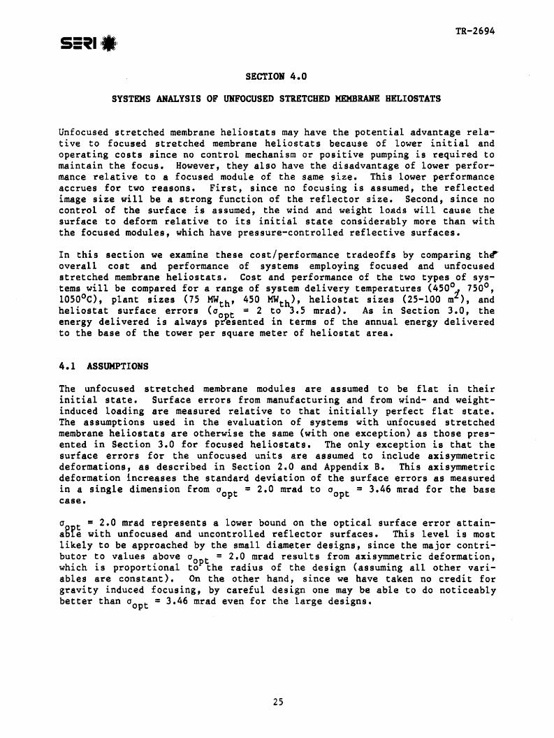
4-6 Effect of Surface Errors on the Annual Energy Delivery forSeveral Sizes of Unfocused Stretched Membrane Heliostats in a75-MW Plant at 7500C Delivery Temperature ••••••••••••••••••••••••••• 31

xi

TR-2694

LIST OF FIGURES (Continued)

4-7 Effect of Surface Errors on the Annual Energy Delivery forSeveral Sizes of Unfocused Stretched Membrane Heliostats in a450-MW Plant at 7500 c Delivery Temperature •••••••••••••••••••••••••• 31

A-l Definition of the Surface Normal Error •••••••••••••••••••••••••••••• 38

A-2 Comparison of the Deterministic Surface Normal Error Distributionand a Circular Normally Distributed Approximation forn • 3and b= 0..................................................... 42

A-3 Comparison of the Density and Distribution Functions forn • 2, 3, and 4, when b =0••••••••••••••••••••••••••••••••••••••••• 42

A-4 Comparison of the Deterministic Surface Normal Error Distributionand a Circular Normally Distributed Approximation for c = 0••••••••• 44

8-1 Assumed Uniform Pressure Loading on the Double MembraneCollector........................................................... 52

8-2 Effective Expected Module Load Corresponding to AxisymmetricMembrane Deformation as a Function of Zenith Angle forSeveral Membrane Designs •••••••••••••••••••••••••••••••••••••••••••• S4

B-3 Effective RMS Surface Error as a Function of PAX forSeveral Model Designs ••••••••••••••••••••••••••••••••••••••••••••••• 55

8-4 Average Load Corresponding to Asymmetric Loading for SeveralModel Designs ••••••••••••••••••••• ~ ••••••••••••••••••••••••••••••••• 56

8-5 Effective Expected Module Area Load Corresponding toAsymmetric Deformation as a Function of Zenith Angle forSeveral Module Weights •••••••••••••••••••••••••••••••••••••••••••••• 57

8-6 Example of Module Construction•••••••••••••••••••••••••••••••••••••• 58

8-7 Torsional and Flexural Rigidity as a Function of Frame HalfHeight ••••••••••••••••••• '. • • • • • • • • • • • • • • • • • • • • • • • • • • • • • • • • • • • • • • • • • • 59

8-8 Maximum Frame Deflection as a Function of Frame Half Height forSeveral Construction Types •••••••••••••••••••••••••••••••••••••••••• 60

8-9 RMS (Surface Averaged) Error as a Function of Frame Half Height..... 60

8-10 RMS (Surface Averaged) Error as a Function of Total Module Weightper Unit of Reflector Area •••••••••••••••••••••••••••••••••••••••••• 61

C-1 Flowchart of Design Procedure ••••••••••••••••••••••••••••••••••••••• 62

xii

TR-2694

LIST OF FIGURES (Concluded)

C-2 Variation of System Performance with Tower Height ••••••••••••••••••• 64

C-3 (a) Expanded Layout and (b) Isometric View of the Baseline ReceiverCavity Configuration •••••••••••••••••••••••••••••••••••••••••••••••• 66

E-l Cone Containing Scattered Beam about the Specular Direction••••••••• 71

E-2 Fraction of Reflected Energy in a Given Cone Size ••••••••••••••••••• 73

F-1 Isometric View of Alternate Receiver Cavity ConfigurationAllowing Larger Aperture Sizes •••••••••••••••••••••••••••••••••••••• 75

F-2 Fractional Change in Delivered Energy as a Result of theLonger Aperture Sizes Possible with the Reconfigured Cavityfor a 75-MW ~ Plant with 100-m2 Unfocused StretchedMembrane Hefl0stats ••••••••••••••••••••••••••••••••••••••••••••••••• 76

xiii

TR-2694

LIST OF TABLES

9-1 Baseline Surface Quality Assumptions................................. 9

3-1 Levelized Energy Cost Assumptions for Focused Stretched Membrane andGlass/Metal Heliostat •••••••••••••••••••••••••••••••••••••••••••••••• 12

3-2 Error Parameters of Figures 3-3 and 3-4 •••••••••••••••••••••••••••••• 16

A-l Errors Introduced by the Assumption of a Normally DistributedBeam Width when b :II 0•••••••••••••••••••••••••••••••••••••••••••••••• 43

A-2 Root-Mean-Square Error Results ••••••••••••••••••••••••••••••••••••••• 47

A-3 Error Introduced in a Single Dimension by a Normal Approximationwhen b • 0, n =2.................................................... 49

8-1 Selected Wind Velocity Characteristics for Several Locations ••••••••• 54

xiv

TR-2694

SECTION 1.0

IHTRODUCTIOH

This report compares, from a systems perspective, the cost/performance poten­tial for stretched membrane heliostat concepts relative to that of matureglass/metal heliostat concepts. In addition to providing- this comparison, thesystem study perspective is required to improve the accuracy of previous esti­mates of the annual energy delivered by a field of such concentrators. Thisreport also documents the sensitivity of stretched membrane heliostat fieldperformance to variations in numerous system parameters such as applicationtemperature, field size, heliostat module size, reflector surface quality, andfocusing capability.

This work is important in that it puts the glass/metal heliostat and thestretched membrane heliostat on a comparable basis so that research decisionsand priorities can be set for the development of the stretched membrane con­cept. This work will also help us to define and quantify the benefits ofspecific research issues and to identify the critical research and developmentefforts required on the stretched membrane concept.

The need for heliostats with dramatically improved cost and performance isdiscussed by Murphy [1] and is supported by the value-based cost goal analysisdeveloped by a joint industry and DOE cost goal committee [2]. The studiesshow that for initial cost competitiveness in regions with relatively highannual insolation, mass-produced heliostats that have performance levels clos~

to those of the current glass/metal heliostats and cost about $100/minstalled are needed. For more widespread competitiveness with ~ broad rangeof conventional fuels, the required cost is about $50-$60/m installed.Further, the need for and use of low-cost heliostat technology is not limitedto solar thermal power applications but potentially may benefit large-scalephotovoltaic applications as wel~ as daylight applications, where large, low­cost, two-axis tracking platforms can greatly enhance the cost/performance of"such systems.

When mass produced, the glass/metal heliostats may reach t~e $lOO/m2 level,but another approach may be required to reach the $50-$60/m level. Becauseof the promise indicated in earlier DOE studies [1,3], research on thestretched membrane heliostat concept has been under way for some time and hasrecently become a focus of DOE development. In this concept, a high-strengthstructural membrane coated with a highly reflective surface is stretched uni­formly on a structural frame (typically a lightweight, hollow, toroidal struc­ture). The stretched membrane concept is a structurally efficient method ofattaining and supporting a large, optically accurate surface. By supportingthe optical surface with a membrane structure, more of the material can bestressed to higher average levels, resulting in both lighter weight and lowercost structures. Further, the stretched membrane can provide a reflectivesurface that tends to smooth out and attenuate surface irregulari ties ema­nating at the supports as well as other surface perturbations inside theperiphery of the supports. This concept also appears to be especially suit­able for the use of polymer reflectors and polymer structural membranes, whichmay further reduce weight and cost and improve handling at the factory, in thefield, and in transport.

1

TR-2694

Following a presentation and discussion on the anticipated accuracy bounds forindividual stretched membrane heliostat modules, the system evaluations aredescribed.

2

TR-2694

SECTION 2.0

INDIVIDUAL MODULE PERFORMANCE

In this section, we provide a brief overview of performance predictions forindividual modules based on analysis findings from a number of previousstudies. The structural analysis performed to date addresses the likelyeffects of wind and weight-loading environments on the structural/opticalperformance of simple stretched membrane modules as well as some of theimpacts of initial imperfections. Much more detail on the supporting analysisof individual modules can be found in Murphy and Sallis [4], Murphy [5], andMurphy et all [6]. We provide here only a summary of these findings and theassociated impacts relating to the macroscopic optical surface accuracy ofindividual modules.

A significant, though not complete, knowledge base has been developed to pre­dict the structural deformation/response of stretched membrane modules underspecified loading conditions [4,5,6]. It is felt that reasonably accuratepredictions of the optical accuracy for individual modules can be made forspecific configurations and loading on the modules using this knowledge base.It should be noted however, that an optimum configuration has not been definedand that, as with the glass/metal heliostats, the loading environment on con­centrators is never fully deterministic since the wind flow approaching thefield typically can be described only in a statistical manner. The nature ofthe wind environment within the field is not well understood because of theextremely complex turbulent flow that exists there. However, performanceestimates of individual modules can be made by defining some average antici­pated loading and then determining the response of the stretched membranemodules to those defined conditions.

Though the major structural response mechanisms have been studied, numerousissues such as module support effects, dynamic effect details, and the effectof anticipated manufacturing tolerances have not been investigated thoroughly.With respect to manufacturing tolerances and initial imperfections, previousanalyses have addressed the amplification effects corresponding to initialimperfections [5] but not the levels that can be anticipated in an actualmanufacturing environment; this issue is currently being addressed throughdevelopment contracts being managed by the Sandia National Laboratories atLivermore (SNLL). This same development activity should also lead to a betterdefinition of the ultimate costs that might be attained with the stretchedmembrane concept. In addition, various static and dynamic structural responseissues are being experimentally investigated. These ongoing activities shouldhelp better define the exact performance of specific designs in the future.

2.1 OPTICAL QUALITY AND SOURCES OF ERROR

The optical quality of a reflector can be defined as the ability of thereflector to redirect incident solar beam radiation in a specular manner to agiven specified target area. A number of error sources that limit that abil­ity are associated with the concentrator. Major sources of error inclUde themacroscopic surface waviness effects, speculari ty effects, tracking errors,

3

TR-2694

pointing errors, loss of hemispherical reflectivity, and the finite sunsize.*' All of the above effects, except for loss of hemispherical reflec­tivity, can be viewed as broadening or scattering effects of the redirectedradiation.

Macroscopic surface waviness gives rise to variations in the direction of thesurface normal and can be induced by a large number of phenomena. Theseinclude the inherent variations in the smoothness of the material surface,structural deformations caused by wind and weight loading, and variations inthe thicknes s of one or more component layers (such as the adhesives) thattypically make up the reflective surface.

The macroscopic surface waviness is impacted in numerous ways by the manufac­turing process. For instance, the accuracy with which the component parts,such as the frame and membrane, can be fabricated before their assembly iscompleted is extremely important in determining the optical quality of theassembled product (e.g., the planarity of the frame before attaching themembrane to it, or the flatness of the strips that compose the elements of themembrane before being seamed to form the final large sheet). Moreover, theuniformity of the thickness of the material stock in the basic membrane mate­rial can also have a significant impact, as can anisotropic material pro­perties in the sheet material. In addition, the method of assembly and mate­rials used in joining the component elements into the final product are ofconcern. For instance, the way the frame is compressed and constrained duringthe attachment of the membrane to it can affect the level to which initialimperfections are amplified by the membrane tension.

As noted above, these questions are now being addressed in development con­tracts managed by SNLL. We are encouraged initially at the prospects for goodmacroscopic optical quality, since the current contractors are optimisticabout their ability to manufacture high quality optical surfaces. We are alsoencouraged that the simple nature of the reflector, the low number of parts tobe assembled, and the inherently forgiving nature of the structure will leadto good macroscopic surface quality for the manufactured module.

Microscopic surface specularity effects cause scattering such that an incomingbeam is not reflected in a single ray but rather as a cone of rays whose sizedepends on the microscopic surface qualities. In good reflectors most of thereflected energy is confined within a very small cone (usually a few milli­radians in width) about the nominal reflected ray (specular direction). How­ever, even for fairly good reflectors, a small amount of energy can be scat­tered at very large angles, resulting in a loss of energy at the receiver.Loss of hemispherical reflectance is caused by absorption of the incoming raysat the surface so that a finite portion of the incoming beams is not specu­14rly reflected or scattered but rather is absorbed.

*These issues have been discussed extensively in numerous prior studies[7,8,9] • Another common term often used in the 1i terature is specularreflectivity, which can be defined, as in Pettit et ale [7], as the productof total hemispherical reflectance (a constant) times a geometric distri­bution function that gives the percent of the total reflected energy within agiven cone angle about the specular directions (see Appendix E).

4

TR-2694

Tracking and pointing errors arise because of limitations in positioning thereflector in exactly the desired direction; these errors represent limitationsto the collection system, but are not fundamentally surface quality limita­tions. Similarly, the finite sun image size always causes the reflected imageof the sun to be fini te even if the reflector were otherwi se perfect, andrepresents a fundamental limitation on the concentration of any concentrator.

In this study, we look at macroscopic variations in surface waviness, specu­larity effects, and hemispherical reflectivity (solar averaged reflectivity)effects. Since the anticipated errors caused by surface waviness effects area function of the individual concentrator type and design, we examine themboth in terms of the performance of individual he1iostat modules (Section 3.0)and from a systems perspective. However, since specularity and hemisphericalreflectivity effects are not primarily dependent on the concentrator concept,but rather on the microscopic reflective surface material quality, we look atthese issues only in the systems analysis sections (Sections 4.0 and 5.0). Inthe systems analysis we look at variations from the baseline values assumedfor glass/metal heliostats. In all our analyses all other error sources,including those not associated with the concentrator, such as tower sway (amoving target), tracking errors and foundation motion are assumed to be thesame as for the glass/metal heliostat~.

2.2 MACROSCOPIC SUllFACE ACCURACY 1M WIND AIm WEIGHT ERVIRONMEHTS

We describe the optical accuracy of stretched membrane modules in terms of themacroscopic surface quality of the stretched membrane surface. A measure ofthis macroscopic surface quality is given by the deviation (~) of the surfacenormals from their desired direction. A convenient definition for our pur­poses is the surface-averaged root mean square (RMS) surface slope error givenby

RMS = <;2> 1/2 = [-f41::Af / 2 •

where dA is the differential surface area.

(2-1)

This measure was chosen for two reasons: it is a convenient way to describe,in an average sense, the macroscopic surface quality of the entire collectorsurface; and it can be related to the probabilistic reflected beam scatteringerror measures typically used in analysis tools such as DELSOL2 [10]. InAppendix A we compare the normally distributed error models of tools such asDELSOL2 [10] with the deterministic distribution of errors over the stretchedmembrane surface. The comparison is made by assuming that the RMS surfaceslope error modeled by a circular normal probability distribution is equal tothe RMS surface slope error as calculated from the deterministic approach.Appendix A shows that the circular normal distribution approximation isadequate for our purposes since we are trying only to bound the anticipatedsurface errors. The adequacy of this approach is reinforced by the fact thatthe wind and weight load induced surface errors are probablistic with time andare combined with numerous other errors that are also assumed to be circularnormally distributed. For such situations, the Central Limit Theorem statesthat the distribution of a random variable equal to the sum of independentrandom variables (not all necessarily normally distributed> approaches anormal distribution.

5

TR-2694

The cumulative distribution function, F(~) (the probability that the opticalscattering angle is less than ~), of the circular normal probability distri­bution approximation is

F(d =l" l 12 exp -I- ~: ) q,dq,de , (2-2)o ,0 2noopt \2 cropt

where 00pt is the standard deviation of the optical scattering angle asmeasured 1n one dimension (i.e., as measured along a line intersecting andorthogonal to the normal from a perfect he1iostat surface). The circularnormal distribution implicitly assumes that the scattering angle in this onedimension is normally distributed with mean zero and standard deviation cr t(see Appendix A). It can also be shown that for the circular normal dist~f­bution aMS = 12 00pt (see Appendix A). Since we are considering bothspeculari'ty effects and surface ~lope errors in our analysis of individualheliostat module performance, cropt must incorporate both these effects, asfollows:

cropt = ~2 + (2 ad)2 , (2-3)*

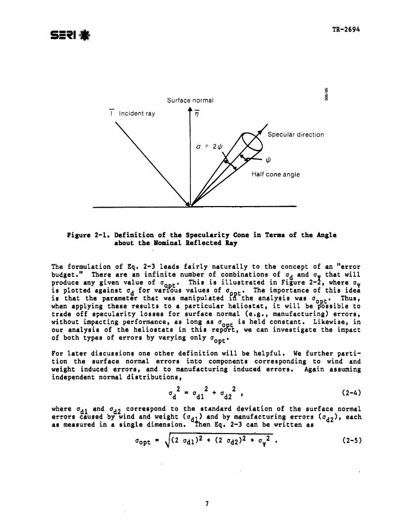
where 0, is the standard deviation of the beam width described by the halfcone angle' (see Figure 2-1) corresponding to specularity effects measured ina single dimension, and ad is the standard deviation of the surface normalerror caused by surface deformation measured in a single dimension.** Thefactor of 2 multiplying ad results from the fact that a surface normal erroris measured from the actual surface normal to the ideal surface normal, andthus produces twice as large an error in the reflected ray. As will be shownin Sections 3 and 4, this factor of 2 produces greater sensitivity of thedelivered energy to surface normal errors than to specularity errors.

In this report , is the half cone angle as measured from the nominal reflectedbeam (see Figure 2-1). The precise defini tion of the angle , is important.Because different conventions are sometimes used in analysis and experimentalwork, the definition of , can lead to confusion. Data from experimentalmeasurements are typically given for the full cone angle a (= 2'). Thisdifference in conventions has evolved since analytical models normally employprobability distributions in which the half cone angle is the random variable,whereas many two-dimensional experiments measure the energy within the fullcone angle. (See Appendix E for more information on specularity and cone sizerelations.)

*We have defined 00 t in this way since the parameters in Eq. 2-3 are theoptical beam spreaating effects, which we vary in this study. Other errorssuch as tower sway and tracking errors are convolved in an analogous manner,and normal values suggested in DELSOL2 were assumed and used throughout.Further sun size effects and collector size effects that also give rise tobeam broadening are handled separately in DELSOL2.

**OELSOL2 requires that surface normal slope errors and specularity errors becombined and expressed in terms of the standard deviations of the surfacenormal error in the two principal heliostat surface dimensions, a~ and a~.

Thus for a circular normal distribution 0opt/2 = a~ = o~.

6

TR-2694

Surface normal

Incident ray

Specular direction

Half cone angle

Figure 2-1. Definition of the Specularity Cone in Terms of the Angleabout the Hominal Reflected Ray

The formulation of Eq, 2-3 leads fairly naturally to the concept of an "errorbudget," There are an infinite number of combinations of 0d and 0, that willproduce any given value of 00 t' This is illustrated in Figure 2-2, where a,is plotted against 0d for varfous values of 0ppt' The importance of this ideais that the parameter that was manipulated 1ft the analysis was 00 t' Thus,when applying these results to a particular heliostat, it will be ~ssible totrade off specularity losses for surface normal (e,g" manufacturing) errors,without impacting performance, as long as CoPt is held constant, Likewise, inour analysis of the heliostats in this rep~rt, we can investigate the impactof both types of errors by varying only Copt'

For later discussions one other definition will be helpful, We further parti­tion the surface normal errors into components corresponding to wind andweight induced errors, and to manufacturing induced errors. Again assumingindependent normal distributions,

(2-4)

where adl and ad2 correspond to the standard deviation of the surface normalerrors caused by wind and weight (adl) and by manufacturing errors (od2)' eachas measured in a single dimension, Then Eq. 2-3 can be written as

(2-5)

7

TR-2694

-.\

\

---

.....-"'C0.0L.e-

~1I'l

b

~ ....0L.L.

WC"')

>....'i: N0

"'5ue-e,

.."

0

0 1 :2 3

Surface Normal Errors, (j d' (mrad)(j opt • 2,0 ----2'..U t_ .~_~.!•.o__

~.uL.~~.JL._

Figure 2-2. Specularity Errors VI. Surface Bormal Error. for a GivenLevel of Total Surface Error Showing the Tradeoff betweenSpecularity and Surface Errors

2.3 ASSUMPTIOIlS FOil INDIVIDUAL MODULES

The basic configurations and characteristics of the individual heliostatmodules considered in the system studies are described below, and the corre­sponding optical performance parameters used in the systems studies are sum­marized in Table 2-1.

The !i-ass/metal heliostat used as the baseline standard of comparison is a100-m rectangular design with twelve facets which are assumed to be focusedand canted at the slant range. In previous systems studies [11] that con­sidered this heliostat, the standard deviation corresponding to the combinedeffects of wind, weight, specularity lost, and manufacturing error is assumedto be given by a t = 2.0 mrad. If we use a baseline assumption ofa, :I 0.5 mrad per 'ittit et ale [7], Eq. 2-3 implies ad :I 0.968 mrad. Thisvalue then accounts for the combined effects of wind, weight, and manufac­turing errors.

The optical performance parameters for the stretched membrane modules arebased on the analyses of "typical tt (adequate, but not optimal) designs withthe structural response characteristics defined by Murphy et ale [4,6]. Ananalysis of the optical performance using these structural response charac­teristics is presented in Appendix B. The results show that the response tothe expected pressure and weight loading drives the design, and also theanticipated optical performance. Appendix B also shows that this response isdifferent for the focused and unfocused modules. The total module weight isshown to be the major design consideration for the asymmetric deformation

8

Table 2-1.

Error Source

TR-2694

Baseline Surface Quality Assumptions

2 2 100-m2 Unfocused100-m 100-m FocusedGlass/Metal Stretched Membrane (Ideally Flat)

Stretched Membrane

0, Hemisphericalreflectivitya

0opt' Wind & Weightmanufacturing/assemblyspecularity (mrad)

0.89

2.0

0.89

2.0

0.89

aAssumes a 0.05 allowance for average dirt accumulation. The reflectance for aclean mirror is assumed to be 0.94.

bAssumed relative to the perfectly flat state.

induced by noncontinuous supports. However, for the axisymmetric membranedeformation of the unfocused module, the wind effect is the major designdriver. This axisymmetric deformation, however, can be eliminated throughactive control in focused modules, which is an important assumption used forthe focused modules.

For the focused module we found the RMS value of the slope corresponding towind- and weight-induced errors to be about 0.50 mrad (see Ap2endix B). Thisresults in a corresponding standard deviation of adl =0.50//2. This wouldimply by Eq. 2-5, assuming a value of 00 t =2.0 mrad and 0 = 0.5 mrad, thatthe standard deviation of manufacturinl errors is 0 2 = 0.927 mrad , Thisappears quite reasonable relative to the glass metal heYlostats where the com­posite ad = 0.968 mrad, since the bulk of the surface errors can be allocatedto the manufacturing error~

For the unfocused modules, which are assumed to be flat in their perfect con­dition, we found (see Appendix B) the upper bound of the RMS value of theslope error corresponding to wind and weight induced errors to be about2.06 mrad.* This results in a corresponding adl = 2.06/ /2 = 1.46 mrad. Ifwe then assume a, =0.5 mrad, and the same manufacturing error as that corre­sponding to the focused modules, (ad2· 0.927 mrad), then a t = 3.46 mrad.This was used as the baseline value for the unfocused designs ?~ee Table 2-1).

Consistent with the analyses provided in Murphy [5] and Murphy et all [6] andin Appendix S, the following assumptions are made:

• The stretched membrane concepts are assumed to be of the double membranedesign, to have a circular shape, and to have three evenly spaced supportsaround the circumference whether the module is focused or not. The doublemembrane selection for the unfocused design is consistent with thestructural efficiency arguments in Murphy [5] and Murphy et all [6].

*RMS2 =RMSix + RMSls = 22 + (0.5)2, where the subscripts AX and AS correspondto the axisymmetric and asymmetric contributions, respectively.

9

TR-2694

• Various module sizes are consi~ered for the stretched membrane conceptbut the baseline assumed is 100 m (11.28-m diameter). It should be notedthat the error approximations established in Appen1ix B and noted inTable 2-1 are based on extensive analyses of a 78-m (lO.O-m diameter)design. It is not anticipated that these approximations should changesignificantly with the 11.28-m design. However, for sizes significantlysmaller the current error estimates will be conservative. This is espe­cially true for the axisymmetric deformations considered with the non­focused designs.

• Designs using steel for both the frame and membranes were assumed sinceit is the most common construction material. However, the lighter mate­rials appear to offer some advantage, and the error approximations givenhere may be somewhat high for these lighter designs.

• For the unfocused design the error caused by the axisymmetric deformationof the reflector membrane must be considered, and is added in quadrature tothe asymmetric error caused by the out-of-plane frame distortion. Areasonable upper bound estimate for this axisymmetric error is assumed tobe RMSAX = 2 mrad per the analysis presented in Appendix B. The error isassumecr-to be measured relative to a perfectly flat condition, and thus nocredit for the weight induced focusing of the reflector membrane isconsidered. Since a number of other conservative assumptions are also madein Appendix B, the performance appears to be bounded by considering RMSAXto be between zero and 2 mrad for the axisymmetric displacements.

• For the focused stretched membrane heliostat, the control scheme proposedby SNLL is assumed to be operative, and is further assumed to be effectivein controlling the axisymmetric membrane deformations to negligiblelevels. In the SNLL approach, an actively controlled pressurel deformationmechanism controls the pressure level within the plenum chamber separatingthe two parallel membranes, such that the axisymmetric deformation in thereflector membrane caused by wind induced pressure is exactly balanced bythe internal pres sure within the chamber. Thus in thi sease, only theasymmetric deformation caused by the frame deformation between the supportsis considered (i.e., RMSAX = 0 and the error corresponding to wind andweight loading is assumed to be RMS =RMSAS = 0.5 mrad).

10

TR-2694

SECTION 3.0

SYSTEMS STUDIES ON THE FOCUSED STRETCHED MEMBRANE MODULE

In this section we describe the systems tr~deoffs for the focused stretchedmembrane heliostats relative to the 100-m, second-generation glass/metalheliostats. The performance issues we investigate include the sensitivity ofsystem cost and performance to (1) stretched membrane module size, (2) surfacenormal errors on the stretched membrane reflective surface, (3) loss of specu­larity on the stretched membrane reflective film, (4) loss of reflectivity forthe stretched membrane module, and (5) cost of the stretched membrane module.The tradeoffs between focused and unfocused modules are discussed in Section4.0.

3.1 ASSUMPTIONS AND GROUND RULES

In many of the comparisons we normalize the energy delivered by the stretchedmembr~ne heliostat with the energy delivered by the corresponding baseline100-m glass/metal he1iostat. The energy delivered is always described on anannual basis and given per square meter of the heliostat being considered.Only IPH systems are considered, and system temperature refers to the temper­ature of the energy delivered at the base of the tower, which is assumed to bethe same temperature as that at the outlet of the receiver. In addition thefollowing assumptions are made.

••

•

•

•

•

The he1iostat optical performance characteristics are as described inSection 2.0.

We consider system sizes of 75, 225, and 450 MWt h with the correspondi~g

approximate field sizes of 100,000, 300,000, and 700,000 m ,respectively.

Average absorber temperatures of 3000, 600°, and 900°C were used in the

analysis. Fur the gurpose of comparison, these are listed as deliverytemperatures of 450 , 7S00 , and 10S00C, respectively. These deliverytemperatures assume a nominal temperature rise of 300°C across theabsorber.

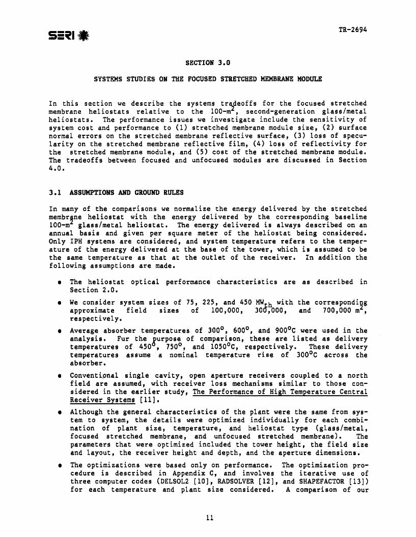
Conventi.onal single cavity, open aperture receivers coupled to a northfield are assumed, with receiver loss mechanisms similar to those con­sidered in the earlier study, The Performance of High Temperature CentralReceiver Systems [11].

Although the general characteristics of the plant were the same from sys­tem to system, the details were optimized individually for each combi­nation of plant size, temperature, and heliostat type (glass/metal,focused stretched membrane, and unfocused stretched membrane). Theparameters that were optimized included the tower height, the field sizeand layout, the receiver height and depth, and the aperture dimensions.

The optimizations were based only on performance. The optimization pro­cedure is described in Appendix C, and involves the i terat i ve use ofthree computer codes (DELSOL2 [10], RADSOLVER [12], and SHAPEFACTOR [13])for each temperature and plant size considered. A comparison of our

11

TR-2694

optimization procedure with a combined cost/performance optimization ispresented in Appendix D.

• The field performance parameters required by DELSOL2, but not describedwith respect to the optical performance characteristics above, areassumed to be the DELSOL2 default values. These parameters include errorestimates for tower sway tracking errors, and sun angle effects.

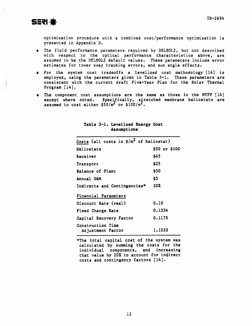
• For the system cost tradeoffs a levelized cost methodology [14] isemployed, using the parameters given in Table 3-1. These parameters areconsistent with the current draft Five-Year Plan for the Solar ThermalProgram [14].

• The component cos t as sumptions are the same as those in the MYPP [14]except where noted. Specifically, stretched membrane heliostats areassumed to cost either $50/m2 or $lOO/m2•

Table 3-1. Levelized Energy CostAssumptions

Costs Call costs in $/m2 of heliostat}

He1iostats

Receiver

Transport

Balance of Plant

Annual O&M

Indirects and Contingencies*

Financial Parameters

Discount Rate (real)

Fixed Charge Rate

Capital Recovery Factor

Construction TimeAdjustment Factor

$50 or $100

$45

$25

$50

$5

20%

0.10

0.1334

0.1175

1.1033

*The total capital cost of the system wascalculated by summing the costs for theindividual components, and increasingthat value by 20% to account for indirectcosts and contingency factors [14].

12

TR-2694

~-r--------------------------.,

3.2 RESULTS FOR FOCUSED MEMBRANE MODULES

In this section we present sensitivity results for the numerous heliostatpar ame t er s and system costs. For each parameter examined we first addressperformance issues and then introduce the cost/performance sensitivities.

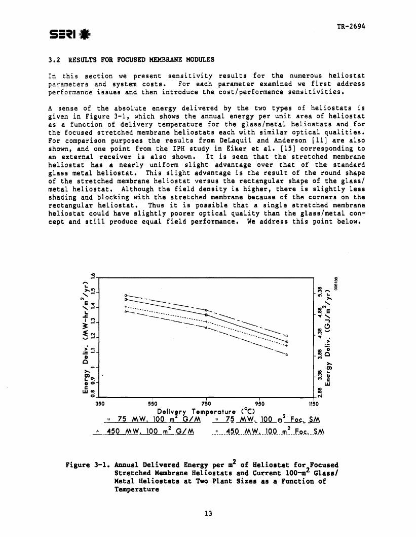
A sense of the absolute energy delivered by the two types of heliostats isgiven in Figure 3-1, which shows the annual energy per unit area of heliostatas a function of delivery temperature for the glass/metal heliostats and forthe focused stretched membrane he1iostats each with similar optical qualities.For comparison purposes the results from DeLaquil and Anderson [11] are alsoshown, and one point from the IPH study in Eiker et all [15] corresponding toan external receiver is also shown. It is seen that the stretched membraneheliostat has a nearly uniform slight advantage over that of the standardglass metal heliostat. This slight advantage is the result of the round shapeof the stretched membrane heliostat versus the rectangular shape of the glass/metal heliostat. Although the field density is higher, there is slightly lessshading and blocking with the stretched membrane because of the corners on therectangular heliostat. Thus it is possible that a single stretched membraneheliostat could have slightly poorer optical quality than the glass/metal con­cept and still produce equal field performance. We address this point below.

~

= ~M _

an ;.......

lC'le.,; ........,co"M-~ .

>='i~c

>-.

>-. =~e- ~ ~GO W

~= Io ........ ----r ...,- ------4-N

350 550 750 950 1150

Dellv!ry Temperature Cae)D 75 MW, 100 m G/M ~~ MW,- 100 ~2 Foc~ SM

_A.~.<LMW.----lO~~.GI.M __~_~_~~.O. __~_W_I._JO_Q I!\_~ __fJ~_~~ __SM

Figure 3-1. Annual Delivered Energy per m2 of Heliostat for FocusedStretched Membrane Heliostats and Current lOO-m2 GlasslMetal Helioltats at Two Plant Sizes as a Function ofTemperature

13

TR-2694

In Figure 3-2 the annual energy delivery for the focused stretched membraneheliostats is normalized to that for the glass/metal heliostats and plotted asa function of the stretched membrane heliostat area.* These results show thatwithin the limitations of the DELSOL2 [10]** code and the range of plant sizesstudied, there is no significant size effect for the focused stretched mem­brane heliostat. This finding was used to simplify our subsequent analysisand comparisons in which we consider only lOO-m2 focused stretched membraneheliostats. (It should be noted that size is an important consideration forthe unfocused stretched membrane. This is discussed in Section 4.0.)

12525 SO 75 100Hellostat Size (m2

)73 loA W Plant ~O_ loA W -Plant _

~~e .NO

"0EN.. .0°4-----.....,-----......-----_----_-------'Z 0

>-'N.. ...:~--------------------------.....,e ~

~ ~-;C_

>-.CD..e.~o

Figure 3-2. Annual Energy Delivered as a Function of Focused StretchedMembrane Heliostat Area. The delivered energy results arenormalized with the 100-m2 glass/metal focused heliostat.

*This is a common form of pee sentat.Lon in this report. The resulting ratiowill be referred to as the "Normalized Annual Energy Delivery."

**OELSOL2 [10] does not handle the astigmatic effect correctly. However, whe~

the focused stretched membrane is of the same order of size as the 100-mglass/metal concepts, the relative effects should be similar in magnitude forthe two concepts. For smaller sizes of stretched membranes there may beanother slight advantage for the stretched membrances when compared to theglass/metal concepts.

There is evidence in an earlier report [11] that for very small plant sizes(5 MW) the size of focused heliostats does have a somewhat greater effect onthe performance.

14

TR-2694

Figures 3-3 and 3-4 show the performance sensitivity of the stretched membranesystew as the surface error is increased beyond the bas! line levels. For the100-m focused stretched membrane heliostats and 100-m glass/metal modules,Figures 3-3 and 3-4 show the normalized annual energy as a function of thestretched membrane heliostat surface error for several values of the deliverytemperature. Figure 3-3 is for a 75-MWt h plant, and Figure 3-4 for a 450-MWt hplant. Both plant sizes show a signiflcant performance drop-off as the totalsurface error is increased from the nominal value of C t = 2.0 to a t =4.80. Note that although there is much less effect witCW temperature pgr agiven value of Co t' the high temperature systems are more sensitive to adecrease in the op~lcal quality than the lower temperature systems. This isbecause of the tighter focusing requirements caused by the smaller aperturesrequired at higher temperatures.

The values of Copt in Figures 3-3 and 3-4 correspond to the RMS error levelsshown in Table j-2. Table 3-2 also shows the corresponding value of Cd' thestandard deviation due to surface deformation (computed from Eq. 2-2, assumingthe standard deviation due to specularity, cy ' is 0.5 mrad). A comparison ofthe first two cases (co t = 2.0 mrad, the base case, and Co t = 3.46 mrad )indicates that a 77% in~rease (1.712/0.968) in the standard 1eviation of thesurface slope error, ad' yields only a small decrease «5%) in the annualenergy delivered.

~.~.

2 3 ~

Surface Errors. (j opt:. (mrad)lJ 450 °c _o_/~O °c

_~.lQ.~JL.oC

>"C"l"- ...:......----------------------------,~ g> ~

1)C>.....:C)"­~e

w

"'E-~ec

-e~o:~o

.~

"'Ee,,-coo ci-+-----------r------~-----.....,.---------4Z

Figure 3-3. Annual Energy Delivered by Stretched Membrane Heliostat Systemswith Various Levels of Surface Error, Normalized by the AnnualEnergy Delivered by State-of-the-Art Glass/Metal Heliostat Systemfor a 75-MWt h Jlant. Both heliostat types and had reflectiveareas of 100 m , appt for the glass/metal heliostat was assumedto be 2.0 mrad. The surface errors are assumed to include bothsurface waviness and specularity effects.

15

TR-2694

52 3 ~

Surface Errors. (j ope. (mrad)c -450 °c _o_'~O °c

_6_.lQ.~~.oC

>-'N... ..:,....--------------------------: ;- ~"iQ

>-...:en...•C

w

'0-:::JCC

-<"'00:.0.~o&..... .o 0-1-------.,.--------,-------.,..--------4Z

Figure 3-4. Annual Energy Delivered by Stretched Membrane Heliostat Systemswith Various Levels of Surface Error Rormalized by the AnnualEnergy Delivered by State-of-the-Art Glass/Metal Heliostat Systemfor a 4S~-MWth Plant. Both heliostat types had reflective areasof 100 m , and "0 for the glass/metal he1iostat was assumedto be 2.0 mrad. ~fie surface errors are assumed to include bothsurface waviness and specularity effects.

Table 3-2. Error Parametersa ofFigures 3-3 and 3-4

RMS " c'1'

2.003.464.80

2.834.896.79

0.9681.71212.387

0.502.874.39

aAll errors are expressed in mi1liradians.

bAssumes a, = 0.5 mrad.

cAssumes ad = 0.968 mrad.

In Figure 3-5 the levelized energy cost (LEC) is shown as a function of "oPtfor a 75-MW h plant at 750°C and 1050oC. Simi lar informat ion is shown InFigure 3-6 Eor a 45S-MWth plant. Here two values of stretched membraneheliostat cost ($50/m and $lOO/m2) are used, and for comparjson the LEC costassuming the baseline glass/metal heliostats (at $lOO/m and 750°C) isshown. It is seen that the surface error (as measured by "opt) can be

16

TR-2694

increased nearly 73% relat~ve to the glass/metal value, and stretched membraneheliostats costing $lOO/m would still be cost effective relati2e to theglass/metal units. Further, for stretched membranes costing $50/m , surfaceerror increases of more than 240% relative to the glas s /metal values wouldstill result in cost effectiveness for the stretched membrane concept.

In Figure 3-7 the normalized annual energy (relative to the glass/metalsystem) from a 75-MWt h plant is shown as a function of the standard deviationof the specularity errors, aV ' of the stretched membrane heliostats. InFigure 3-8 the levelized cost o~ energy is shown as a function of a~ for twostretched membrane costs ($lOO/m and $50/m2) and the same plant consldered inFigure 3-7. In both of these plot s the basel ine surface normal errors ofad = 0.968 mrad are assumed to be constant. It is seen that the system ismuch more tolerant of specularity error than of surface deformation asexpressed by ad' which follows from Eq. 2-3. For instance at 6000C increasingthe specularity error standard deviation from 0', = 0.5 mrad to 4.00 mrad whileholding ad = 0.968 mrad has the same effect as changing ad = 0.968 mrad toad = 2.21 mrad while holding a, constant at 0.5 mrad.

-----+

8

--------+---_.. ----

-'--'- ---E:l__ ._" ---Ir -- ---" ______

~ - -'- ---e-- - ------ -------cr--- -

234

Surface Errors, a0 t, (mrad)Cl SM, 750°C, $50/m2 ~M. 1050_oCr $5Q/m2

. ,l._. SM2q~CJ100/m2 ..~_ ..~M/JQ~9__~~t_$1Q_QIJTI~....~ GlM.,..7qO.. ~.C., ..$1.QQ/m.2

r-----------------------------,~ Sl~ ~

...I"'-IO--------.....,.------..,..---------r-------+..t

5

Figure 3-5. Levelized Annual Energy Cost as a Function of Surface Error forthe 75-MW Plant (as in Figure 3-3) at Two Delivery Temperaturesand Two Heliostat Costs. The LEC for the baseline glass/metalheliostat system (at 7500C and $100/m2) is shown for comparison.

17

TR-2694

_,--to-'- ~-1!r"'-'- __

~,--,-,-'-' -­_------e--cr--- -

--+---------

--

.--

-e-

.:«:

.-.- .• -+--_ ........ -

.---------------------------, ;t,...~ Sl

§

~~t.90-......

enoU

'It >"": ~IX) (I)

Lfi~~... "": isco >

.s

Figure 3-6. Levelized Annual Energy Cost as a Function of Surface Error forthe 450-MWPlant (as in Figure

23-4)at Two Delivery Temperatures

and Two Heliostat Costs ($50/m and $lOO/m2). The LEe for thebaseline glass/metal heliostat system (at 7500 C and $lOO/m2) isshown for comparison.

2 3Specularlty Errors a,;j (mrad)

c 450 °c _O_/~O °c_6_.lQ.~JL.oC

o

0-~.

~o

.!:!-0E e... .o 0 -.+------r------,..------r-----....,.------fZ

>.oN... -~--------------------------.,~ ~

~ i"io>.0­D)...~cw ~,~.

~--~-----0-~

cc

-e

Figure 3-7. Normalized Annual Energy Delivery from Focused Stretched Mem­brane Heliostats as a Function of the Standard Deviation ofthe Specularity Errors for a 75-MW Plant at Three DeliveryTemperatures

18

TR-2694

5

-' -+.-­-'-- - - - - - - - --+- --

___ El

___ - __,--,-6______ --e-- -, __ --

~--- _,--tr.---,-'­~-'-'-

+--------

; 2 3 ~

Specularity Errors a (rnrad)a SM, $50/m 2

, 750 °c ~ty1, $100jm 2, 759 °c

_I> . SMJ~.QLm':J050~ __~ ~M~_.sJQQlro~~JQ~O __~~

.,x.. ""GI.M.L$JO'Q/m.~,~..790 ..~.G

V

-+-----...,....----.....,..------r-----,......----+~

-C")

~-...a:l~~........~~...en0

U

~CJ)~

Q)r::w

"C.§ ,...1)>Q)

...J

It)

0

....- --..,v

""~

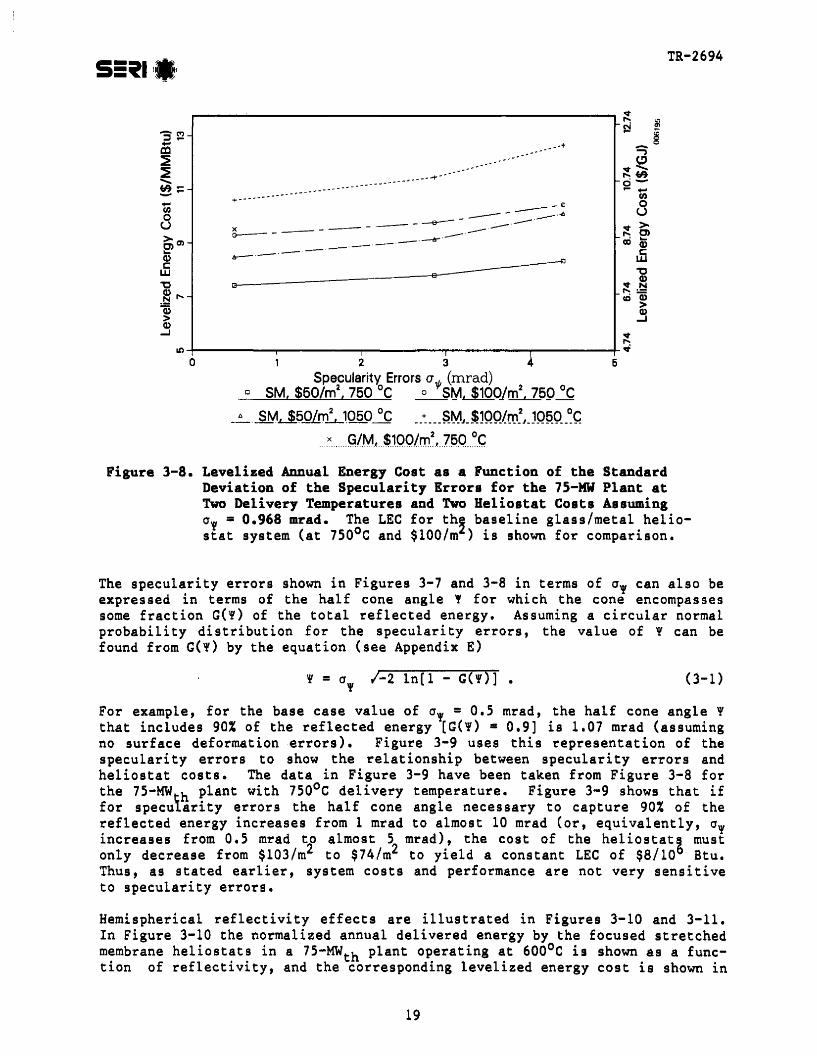
Figure 3-8. Levelized Annual Energy Cost as a Function of the StandardDeviation of the Specularity Errors for the 7S-MW Plant atTwo Delivery Temperatures and Two Heliostat Costs Assumingay = 0.968 mrad. The LEC for th~ baseline glass/metal helio­stat system (at 7500 C and $lOO/m ) is shown for comparison.

The specularity errors shown in Figures 3-7 and 3-8 in terms of a, can also beexpressed in terms of the half cone angle " for which. the cone encompassessome fraction G(,) of the total reflected energy. Assuming a circular normalprobability distribution for the specularity errors, the value of '¥ can befound from G('¥) by the equation (see Appendix E)

(3-1)

For example, for the base case value of a~ = 0.5 mrad, the half cone angle'that includes 90% of the reflected energy [G(Y) = 0.9] is 1.07 mrad (assumingno surface deformation errors ). Figure 3-9 uses this representation of thespeculari ty errors to show the relationship between speculari ty errors andheliostat costs. The data in Figure 3-9 have been taken from Figure 3-8 forthe 75-MW h plant with 7500C delivery temperature. Figure 3-9 shows that iffor speculari ty errors the half cone angle necessary to capture 90% of thereflected energy increases from 1 mrad to almost 10 mrad (or, equivalently, cr,increases from 0.5 mrad t

20 almost 5 mrad ) , the cost of the heliostat~ must

only decrease from $103/m to $74/m2 to yield a constant LEe of $8/10 Btu.Thus, as stated earlier, system costs and performance are not very sensitiveto specularity errors.

Hemispherical reflectivity effects are illustrated in Figures 3-10 and 3-11.In Figure 3-10 the normalized annual delivered energy by the focused stretchedmembrane he1iostats in a 75-MWt h plant operating at 6000 C is shown as a func­tion of reflectivity, and the corresponding 1eve1ized energy cost is shown in

19

TR-2694

- ..- ........ _--t-

-------"---­---- - ----a--

+-._--._----. - -.. ......... -....... -.... --._-._--+••••_-.-..........

-'-'-'- --.-----.._-'--0_,_,_,_-'"""-6

°~I-------------------------~

i

11102 3 4 6 e 789Half Cone Angle, 1/1 (Gy = 0.90)

c LEC == $10/MMBtu ~~C = $9jMMBty

_6,. LEe =,te!MMBtu __-+: k~C_:::__$71MMe.t~

o-t---,..--r--"'I"'---r---r---r----r--..,.---,...----,----1o

rigure 3-9. Allowable Reliostat Cost as a runction of the Specularity BalfCone Anale for Several Lelels of Levelized Energy Cost for a75-MWt h Plant UsiOI 100-. Focused Stretched Membrane Beliostatlat a Delivery Temperature of 7S0oC. This is the heliostat costthat allows you to maintain the given LEe despite increasingspecularity errors.

O.9SO.BSHemispherical Reflectivity

O.7S

>'N~ ...:....,....-----------------------......,e ~

~ i"io>....:CD~

ec

w

'0-:::JCC

-c"'t:'D:eO.~'0E

ID~ .o 0-4-----------"T"""""---------r-------I

Z

Figure 3-10. Normalized Annual Energy Delivery from Focused Stretched M~brane Beliostats as a Function of the Hemispherical Reflectivityfor a 7S-MW Plant at 7S0oC Delivery Temperature

20

TR-2694

r--------------------------__ ~~

A---e-.- _

---~

;!IO-r---------~----------,._----.L~

0,75 0,85 0,95

Hemispherical Reflectivityo SM Hel Cost = $50/m

2~~ Hel Cgst = $jOO/m 2

_t>_. Ba~eline G/M Hel Cos~ =$100/m~

Figure 3-11. Levelized Annual Energy Cost as a Function of the HemisphericalReflectivity for a 75-MW Plant with 750°C Delivery Temperatureand Two Heliostat Costs. The LEC for the baseline glass/metalheliostat system is included for comparison.

Figure 3-12 for the two assumed stretched membrane heliostat costs of $50/m2and $100/m. As might be expected, the decrease in delivered energy is nearlyproportional to the decrease in hemispherical reflectivity.

In the base case the hemispherical reflectivity assumed is the same as that ofthe glass/metal heliostat. However, it may be that environmental degradationof the polymer surface due to ultraviolet radiation, temperature cycles,moisture, and dirt will be more severe than that of a glass/metal surface.The results in Figures 3-10 and 3-11 illustrate the sensitivity to suchdegradation.

The sensitivity of the annual energy delivery and the LEe to changes in thesurface normal, specularity, and reflectivity parameters is shown in Fig­ures 3-12 and 3-13 for two delivery temperatures. Both figures show theresults for a 7S-MW system using 100-m2 focused stretched membrane heliostats.Figure 3-12 shows the sensitivity of the energy delivered per unit area ofhelio~tat (E/A), and Figure 3-13 shows the sensitivity of the LEC assuming$50/m heliostat costs. Clearly, the biggest effect is with variations inhemispherical reflectivity, and the next largest effect is caused by surfacenormal effects. It is seen that receiver temperature causes only moderateeffects. Noting the scale on the ordinate of these plots shows that, in fact,rather dramatic changes in ad and cry have only small «10%) changes in E/A,LEC, and the energy delivered per unit of heliostat area.

21

TR-2694

0.-- ----.Sl§

.!: 0o•enc:o

.J:U

O~c: O.2 I-UoL.

U.

N

tfT----....,-----r------r----~---.....,.---~o 2 3 ~ 5 6

Ratio to Nominal Valuee fJ d for 750°(. fJ '/I • .5 ~!t .19.L L0500C L~ _ .5

_6_.~ ...1.2r___l.50~~.CL!!...~.96~ __: g_'J!__ J9!:. __1Q.~_O_~~l __g_Ij__~ __ !9..6_e...~ R.,JI !;J'.VJ.ty,.~ J?.

'igure 3-12. A Comparison of the Relative Effects of Several Optical Param­eters on the Annual lneraY Delivery for a 75-MW Plant Usina'ocused Stretched Membrane Reliostats. The ordinate shows thefractional change in the energy delivered relative to the base­line, while the abscissa represents the ratio of the independentparameter to its baseline value. The independent parameters arethe surface normal errors, ad (assuming a, = 0.5 mrad), thespecularity errors, a, (assuming ad =0.968 mrad), and thehemispherical reflectivlty, p.

3.3 IMPACT 0' OPTICAL ERROR UHCERTAINTIES

The results presented in Section 3.2 for focused stretched membrane he1iostatsand in Section 4.2 for unfocused stretched membrane he1iostats presume thatthe optical error as represented by aoot is accurately estimated. To derivethese results the energy delivered by rhe system was calculated as a functionof aopt only after the system configuration--fie1d layout, receiver aperturesize, etc.--had been optimized at the assumed error level ao t. If theoptical errors have been misestimated or if they change over tim~, it is pos­sible that the energy delivered by the system will vary considerably from theresults in Sections 3.2 and 4.2.

To investigate the sensitivity of the delivered energy to the uncertainty inthe optical error estimates (i.e., to ao~t)' we conducted a limited number ofsimulations in which the system config\!ration was optimized at one opticalerror level and performance was estimated at a second error level. Theresults of these simulations are illustrated in Figure 3-14, where for a 75-MWplant delivering thermal energy at 4500C we show the sensitivity of systemperformance to optical errors for several optimization assumptions. Theuppermost curve corresponds to the approach used in all of the other analyses

22

No

uW-Jc:.~.- 0

CDC)CCtI..co~OCtICo',p

~"":... 0

U. I

.:-:

_._._.-_.--.-.-

ooNCOoo

TR-2694

N

9-t-------"""T'"--------,-------.,..--------fo 234

Ratio to Nominal Valueo ad for 750°C, a1/; = .5 ~'.! for lO_50oC,

ajl = .5

_A_.!li for 750~.9"d= .968 __~ Q-y,_J9.rJQQQ_o_c;J_~g_:=__:~J?~

x R~fl~G~iyitYr.P

Figure 3-13. A Comparison of the Relative Effects of Several Optical Par~eters on the Levelized Energy Cost for a 75-MW Plant Using$50/m2 Focused Stretched Membrane Heliostats. The ordinateshows the fractional change in the LEe relative to the baseline,while the abscissa represents the ratio of the independentparameter to its baseline value. The independent parameters arethe surface normal errors, ad (assuming a, = 0.5 mrad), thespecularity errors, Of (assuming ad = 0.968 mrad), and thehemispherical reflectivlty, ~.

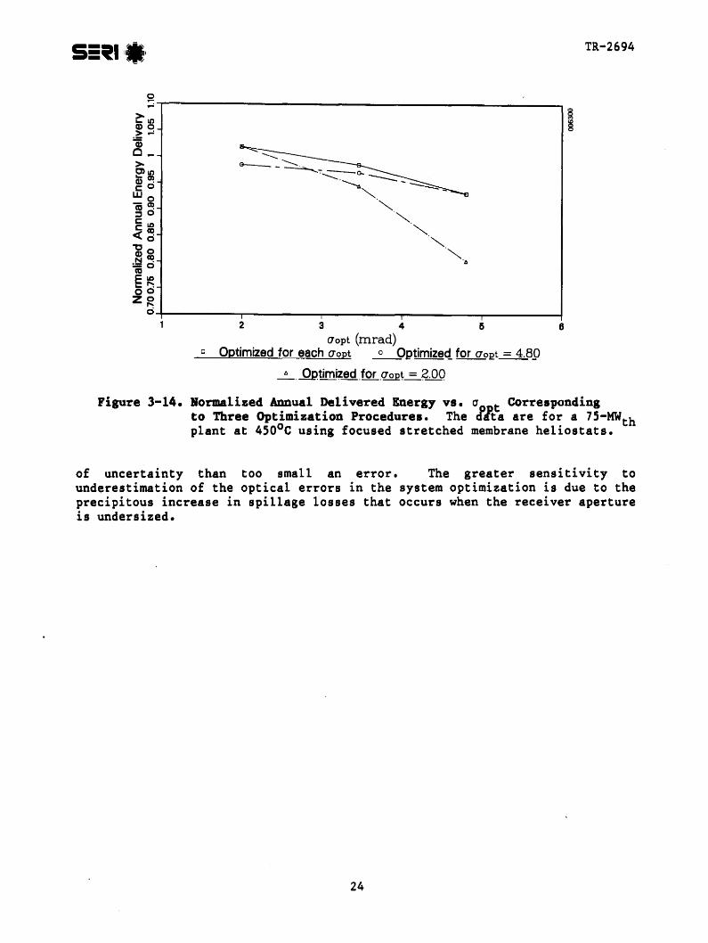
presented in this work (i.e., the system is performance optimized for eachspecific known error). The second curve, which is coincident with the firstcurve at a value of (J p = 4.8 mrad, corresponds to a system configurationthat has been optimizeS for an optical error of (Jopt = 4.8 mrad, after whichthe performance was evaluated at lower optical errors. The third curve, whichhas the steepest slope and is coincident with the upper curve at ao t = 2,corresponds to a system configuration that has been optimiz~d for00Pt = 2 mrad. This same configuration is then held constant while the actualoptlcal error is increased and system performance determined.

Several conclusions can be drawn from this figure. As expected, the systemwith the best performance is that which considers the field/receiver config­uration to be performance optimized at each optical error level (first curve).The performance sensitivity to optical surface errors is greatest for systemsoptimized for too low an error estimate (third curve); the least sensitivityis seen to occur for the system optimized for too high an error (secondcurve) • Thus the penal ty for as sumi.ng too small an error is in generalsignificantly greater than for assuming too large an error. Hence from adesigner's perspective it is better to design for a larger error in the face

23

3.-------------------------_--.~It)CDO>-=

13C_>­C>It)

C5~LEoo

16~::::1 0Cit)Ceo«0"Co~cq

"co 0

E~00zg

O-+-------r------r-----......,.-----..,...- ~23466

Oopt (rnrad)tl Optimized for each Oopt ~ptimizec!for Oopt = 4.8.9

_l>_.J2ptimi~ed ,tor .Cl£12t-=-~.OQ

TR-2694

Figure 3-14. Normalized Annual Delivered Energy vs. a t Correspondingto Three Optimization Procedures. The iita are for a 75-MWt hplant at 450°C using focused stretched membrane heliostats.

of uncertainty than too small an error. The greater sensitivity tounderestimation of the optical errors in the system optimization is due to theprecipitous increase in spillage losses that occurs when the receiver apertureis undersized.

24

TR-2694

SECTION 4.0

SYSTEMS ANALYSIS OF UNFOCUSED STRETCHED MEMBRANE HELIOSTATS

Unfocused stretched membrane heliostats may have the potential advantage rela­tive to focused stretched membrane heliostats because of lower initial andoperating costs since no control mechanism or positive pumping is required tomaintain the focus. However, they also have the disadvantage of lower perfor­mance relative to a focused module of the same size. This lower performanceaccrues for two reasons. First, since no focusing is assumed, the reflectedimage size will be a strong function of the reflector size. Second, since nocontrol of the surface is assumed, the wind and weight loads will cause thesurface to deform relative to its initial state considerably more than withthe focused modules, which have pressure-controlled reflective surfaces.

In this section we examine these cost/performance tradeoffs by comparing thEroverall cost and performance of systems employing focused and unfocusedstretched membrane heliostats. Cost and performance of the two types of sys­tems will be compared for a range of system delivery temperatures (450 0

t 1500 ,

1050 0 C) , plant sizes (15 MWt h, 450 MWt h) , heliostat sizes (25-100 m ), andheliostat surface errors (00 t = 2 to 3.5 mrad}, As in Section 3.0, theenergy delivered is always pr~sented in terms of the annual energy deliveredto the base of the tower per square meter of heliostat area.

4.1 ASSUMPTIONS

The unfocused stretched membrane modules are assumed to be flat in theirinitial state. Surface errors from manufacturing and from wind- and weight­induced loading are measured relative to that initially perfect flat state.The assumptions used in the evaluation of systems with unfocused stretchedmembrane heliostats are otherwise the same (with one exception) as those pres­ented in Section 3.0 for focused heliostats. The only exception is that thesurface errors for the unfocused units are assumed to include axisymmetricdeformations, as described in Section 2.0 and Appendix B. This axisymmetricdeformation increases the standard deviation of the surface errors as measuredin a single dimension from Gopt = 2.0 mrad to 00pt = 3.46 mrad for the basecase.

° t = 2.0 mrad represents a lower bound on the optical surface error attain­agfe with unfocused and uncontrolled reflector surfaces. This level is mostlikely to be approached by the small diameter designs, since the major contri­butor to values above 00pt = 2.0 mrad results from axisymmetric deformation,which is proportional to the radius of the design (assuming all other vari­ables are constant). On the other hand, since we have taken no credit forgravity induced focusing, by careful design one may be able to do noticeablybetter than 00pt = 3.46 mrad even for the large designs.

25

TR-2694

4.2 RESULTS FOR UNFOCUSED STRETCHED MEMBRANE SYSTEMS

Figure 4-1 presents a performance comparison of the three heliostat types con­sidered--glass/metal, focused stretched membrane, and unfocused stretched mem­brane--for the base-case assumptions and delivered energy temperatures from4500 to 10500C and for a 75-MWt h plant size. The top two curves representingthe focused stretched membrane and glass/metal heliostats present the sameresults shown in Figure 3-1. Although the base-case assumptions for thefocused and unfocused results of Figure 4-1 are the same except for the sur­face errors, the system configuration has been reoptimized for each case basedon performance for each heliostat type. The bottom curve r.epresenting theunfocused case indicates that the higher surface errors (aop~ = 3.46) assumedfor this case together with the size effect for the 100-1n flat unfocusedheliostats reduce the delivered energy by 15% to 30% relative to the focusedcase. The greatest reduction occurs at the higher delivered energy temper­,tures because the receiver aperture is smaller and focusing more important.

In Figure 4-2 the annual energy delivered per square meter by a 75-MW unfo­cused stretched membrane heliostat system has been normalized by the annualenergy delivered from a system using 100-m2 focused stretched membrane belio­stats with a t = 2.0 mrad. The energy delivered by the unfocused systemsmare closelyO~pproaches tbat from a focused system (the ratio approaches 1.0)

~----------------------------,

------------...

>-~o:eoc ~w~ ~o+-----.....,r--------,-------r--------t-"

>-eo

350 550 750 950 1150

D.I~v.ry T.mperature ~oC)100 m G/II\ 100_m......£o_c 511\,_<10,.- _2.0 m-:ad

_l()JL.~. Unt_..i~.~~~~.4~__!!!.rad._

Figure 4-1. Comparison of the Baseline Cases for Class/Metal and Focusedand Unfocused Stretched Meaabrane Heliostats. ' The total sur­face errors, a , are 2.00 mrad for the glass/metal and thefocused stretcgCa membrane heliostats, and 3.46 mrad for theunfocused stretched membrane heliostats.

26

TR-2694

-- ..... -- -- -+.

... ---+- ------

-_.- __ t ..· .

._'-._.~

---.---. ---, ---.---.---.~

uo .... ...,..----------------------------,u..

"'­uo~

Co­=>0

1150350

c:~

c: O+------"""""T------~-----__r_---------!-< I

550 750 950

2 Delivery Temperature <;C)[J 25 m Hel.. cropt· 2.00 mrad ~~-.ID..-H_e~o.pt· 3.~t6 mrag

2 2~. 50._m_ti-!.L~--£.~~,~~.mrad __~ ]QQ __m tj~l._.__ 5~_O.P_~~ 3~~~ __mCQ~

Figure 4-2. Ratio of Annual Energy Delivery for the Unfocused StretchedMembrane Heliostats to That for the Focused Stretched Mem­brane Heliostat as a Function of Delivery Temperature for3 Heliostat Sizes and a 75-MW Plant. The total surfaceerrors, 00 t' of 3.46 mrad represent the baseline for theunfocused ~ystems, while the curve for aopt of 2.00 mrad isan upper bound on the reduction in surface errors possiblewith smaller heliostat sizes.

as the size of the unfocused modules is decreased. This illustrates that asthe area (diameter) of an unfocused stretched membrane heliostat is reducedthe losses caused by lack of focusing (heliostat size errors) are reduced.

Note that the delivery temperature also has a significanf effect on the rela­tive performance. At lower temperatures even the lOO-m unfocused stretchedmembrane heliostats can produce about 88% as much energy per unit area as thefocused modules. This is because the lower temperature systems have rela­tively larger apertures and lower thermal losses per unit area of aperture.Therefore, the fractional increase in the optimized aperture area is smaller,and the penalty for increasing the aperture size is also smaller.

Figure 4-3 shows that the heliostat size effect is also much less influentialfor larger plant sizes. The reason for this difference is that, as with thelower temperature systems, the larger plants have intrinsically larger aper­tures, and the fractional increase in the required optimum aperture size isaccordingly smaller.

The bottom three curves in Figures 4-2 and 4-3 are all for a constant value ofao t (= 3.46 mrad). This is equivalent to assuming that a decrease in theheflostat size affects only the size error (the error introduced by the finite

27

TR-2694

~- --:.. -~:----_:-:=----:-~-~:~:=_~:::==-=~.. -........

El8

u

a.f -r----c1f=================s:==::::::=========::;----,.......uo­Co-

::;) 0-I

o:;OGO~ 0-

..C

1150350

c-qc 0-t--------,-------r--------,r-------~-e

rigure 4-3. Ratio of Annual Energy Delivery for the Unfocu8ed StretchedMembrane Belio8tat to That for the Focused Stretched Mem­brane Belio8tat as a runction of Delivery Temperature for3 Belio8tat Sizes and a 450-MW Plant. The total surfaceerrors, 0opt' of 3.46 mrad represent the baseline for theunfocused systems, while the curve for 00 t of 2.00 mrad isan upper bound on the reduction in surfacK errors possiblewith smaller heliostat sizes.

size of the unfocused heliostat) and not the surface errors. In fact, asdescribed in Section 2.0, the surface errors will also probably decrease withdecreasing heliostat size. The top curve in both figures presents a likelyupper bound on the performance improvement possible with smaller unfocusedheliostats. since it incorporates a reduction of the surface errors to thesame level as that assumed for the base-case focused heliostats(oopt. = ~.OO mrad). Note that in this case the decrease in performance forthe 25-m unfocused heliostats relative to the focused heliostats is onlyabout 3% for the 75-HW system operating at 4500C, and less than 1% for the4S0-HW system. Thus, if these errors could be achieved, the performance ofsmaller unfocused heliostats could effectively equal that of the state-of-the­art glass/metal heliostats.

The results presented in Figures 4-2 and 4-3 are transformed into a comparisonof the relative economics of focused-versus-unfocused stretched membraneheliostats in Figures 4-4 and 4-5 (i.e., how much more one could afford to payfor focused heliostats without increasing the levelized cosi of deliveredenergy). The unfocused heliostats were assumed to cost $50/m , and the eco­nomic assumptions were taken from the current Multiyear Program Plan [14]. Inessence, Figures 4-4 and 4-5 show that, depending on the situation, unfocusedheliostats begin to be advantageous if the incremental cost of the focusing

28

TR-2694

~...,.------------------------~--....,

--------­_ ----e-------..­--'..-..-

ojo - -'

.....--,.....--.~

.....-- ......--'.....-­.....--'

-'~'-'-'-----o...J-,--......,..---~--"""T'"---.,----r-----,.---.,.-----t

360 460 660 660 760 860 960 1060 1160

2 Delivery Temperature (°9Cl 25 m , aopt= 2,00 rnrad ~g rrLJ!qpt= 3.4.9 rnraq

2 2_"'_, 50.m...cQ.QRt= ,3.46_rnrad __~ __JQ~Lm_J __q9.E~::_~·:Htmrs:!g

Figure 4-4. Allowable Cost of Focusing as a Function of DeliveryTemperature for a 75-MW Plant at Several HeliostatSizes and Total Surface Errors. The allowable cost offocusi2g is the increase in the cost of the he1iostats(per m ) you could afford for focusing without increas-ing the 1evelized energy cost. These va1~es are based on aconstant unfocused heliostat cost of $50/m •

(above the cost of comparable unfocused heliostat) exceeds about $4-$5/m2 forthe cases with the larger surface errors (ao t = 3.46). However, if thesurface errors on the unfocused he1iostats caW be reduced to those of thefocu~ed module (oQpt_= 2) the allowable cost of focusing drops to less thanSlIm for the 450-MWt h plant. As with the earlier results, the figuressupport the conclusion that the unfocused heliostats appear to be advantageousfor larger plants, lower temperatures, and for smaller heliostat sizes.

One assumption implicit in the analysis behind Figures 4-4 and 4-5 is thatheliostat cost per square meter is independent of heliostat size. Clearlythis assumption ignores the increase in the number of supports, trackingmechanisms, and controls that accompany a decrease in the size of the helio­stat (and a corresponding increase in the number of heliostats).*

*Additionally, it could be argued that some extra controls would be requiredfor emergency defocusing of the unfocused heliostats. This is because in anemergency (e.g., loss of fluid in the absorber) the beam from the focusedhe1iostats can be quickly dispersed merely by eliminating the vacuum (or evenpressurizing) in the space between the membranes. However, with the unfocusedstretched membrane heliostats (as with the glass/metal heliostats currently inuse) the heliostats must actually move off their aim point in order to defocusthe field.

29

TR-2694

~ .....----------------------------.

":LD5 ....U

••••••• --+........

I I

4150 15150 660 760 860 960 10150 1160

2 Delivery Temperature (°9o 25 m , Gopt= 2.00 mrad ~Q~~t= 3.41> mrag

2 2_11_. 50,l!L, Gopt= .3.49 mrad __~ __ JQQJII_J_.Q'PJ2t:::_9A-{tmr~g

Figure 4-5. Allowable Cost of Focusing as a FunctioD of DeliveryTemperature for a 450-MW Plant at Several Helio.tatSizes and Total Surface Errors. The allowable cost offocusi~g is the increase in the cost of the heliostats(per m ) you could afford for focusing without increas­ing the levelized energy cost. These values are based ona constant unfocused heliostat cost of $SO/m2•

Nonetheless, the results presented should be useful as guidelines as long asthe total installed cost per square meter is used in the comparison.,

Although the size error introduced by unfocused stretched membrane heliostatscan be large relative to the surface. normal and specularity errors, the per­formance of a system with unfocused heliostats is essentially just as sensi­tive to surface normal and specularity errors as a system with focusedheliostats. Figures 4-6 and 4-7 compare the decrease in performance for thesetwo types of heliostats as a function of the combined surface normal andspecularity errors COopt) for several sizes of unfocused heliostats.

The results for the 75-MW system in Figure 4-6 show that the difference inheliostat size errors nearly overwhelms any difference caused by the surfaceerrors. However, in Figure 4-7 the resul ts for the 450-HW system indicatethat the two error sources cause about the same magnitude of decrease in per­formance for the ranges studied.

The results presented here indicate that smaller plant sizes are significantlymore sensi tive to decreases in the optical qual i ty of the reflected beam(caused by either surface errors or size effects) than larger plants. To someextent, this increase in sensitivity is exaggerated because the receiver usedin all of the cases presented in Sections 3.0 and 4.0 was a general cavity

30

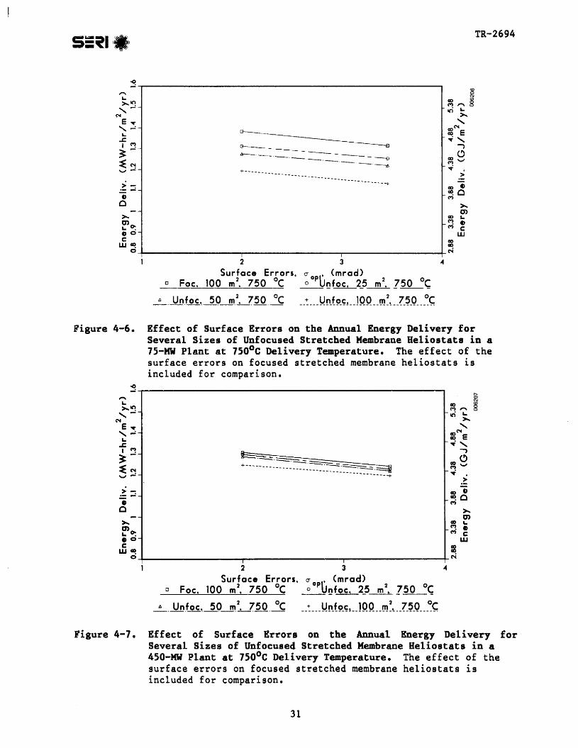
SL.-~I ."- II II- "_7

TR-2694

~-r-------------------------------.-L>-~­,-

N

e~, ...:-L

.s:I ~_

~-

~ ~-

>­= ~-

~___ --S

I!:r---. _~_._, ---=-~ - --£)

-'-'-- -'-+---- -. ----- --------------t

<0

~

~",,8lri ;..

<,~Ne~,...,CID"M-~ .

>CID G)~OM

I I

234

Surface Errors, cr p' (mrad)[J Foe, 100 m2, 750 °c ~~~2_5~ 750 0c;

_t._,JlD,foc~~O---.m,~50, °c __~ __ J.htt9_~!_JQ~L_m~Ll_~_Q ~<;

>--- ~>- CID L

~~ ~ G)CJO- L.5c CIDW~ CIDO-+- ~--------_.,..--------___+_N

Figure 4-6. Effect of Surface Errors on the Annual Energy Delivery forSeveral Sizes of Unfocused Stretched Membrane Beliostats in a75-MW Plant at 750°C Delivery Temperature. The effect of thesurface errors on focused stretched membrane heliostats isincluded for comparison.

I I

2 3

Surface Errors, cropt'. (mrad)[J Foe, 100 m2, 750 °c _o__u~foc, 2_5~750 0<;

_A_. Un,foc~~O_.ID,~50.°c __~ __J.htt9_~1_JQQ __m~Ll_~_Q ~~

~-r------------------------------,~ 8~M_

f-lri ;..,~tef-~,...,

1100

(")-

~ .>

~"i~oM

.~ a."io ~-- ~~ 110 L.

~o: f-~ ~It 0- W

~~ io+- --po ---, +N

""L>-1l1_,-

N

e~, ~-

L..s;

i ~-

~ C"!_--

Figure 4-7. Effect of Surface Errors on the Annual Energy Delivery forSeveral Sizes of Unfocused Stretched Membrane Heliostats in a450-MW Plant at 750°C Delivery Temperature. The effect of thesurface errors on focused stretched membrane heliostats isincluded for comparison.

31

TR-2694

configuration originally designed for high temperatures and relatively highabsorber plane flux levels.

Unfortunately, a single receiver configuration cannot cover the entire rangeof potential applications. In this case, the particular geometry chosen couldnot simultaneously accommodate both the desired absorber flux levels and thelarge apertures required to optimize the unfocused, poor optical qualitycases. Because of this limitation, another receiver design was brieflyinvestigated that outperformed the base-case receiver for these cases. Thegeometry of this receiver and an example of the potential improvements inperformance are given in Appendix F.

Even with this exaggerated decrease in performance at the smaller plant size,the unfocused stretched membrane heliostats demonstrate a remarkable level ofperformance, competing well with both the focused stretched membrane helio­stats and the glass/metal heliostats in a significant number of cases. Thechoice of focused-versus-unfocused designs for a system designer will clearlydepend strongly on the particular application. In terms of the Solar ThermalProgram, the focused stretched membrane heliostats show a promise for applica­bility over a broader range of applications, and would probably be favored onthat basis.

32

TR-2694

SECTIOII 5.0

CONCLUSIONS

In these systems comparisons of stretched membrane heliostats with glass/metalconcepts we have investigated a wide range of system and component parameters,including variations in system operating temperature, system size, heliostatsize, macroscopic surface normal errors, specularity, and hemisphericalreflectivity. Considering the range of temperatures and system sizes investi­gated, the current study provides information on a larger range of sensitivityvariations than any other previous documented study of heliostats, whetherglass/metal or stretched membrane.

In support of the systems studies, the major findings from recent and ongoingstructural and optical response investigations of individual stretched mem­brane modules are cast in terms of performance parameters needed to describecollector field performance. As such, the current study integrates a largenumber of results and definitions from systems, structural, and optical mate­rials studies into a single unified presentation.

Based on the range of parameters described above, it appears that focusedstretched membrane heliostats may have performance levels that are quite closeto and possibly slightly better than the corresponding glass/metal heliostats.This is due to their apparent ability to maintain good macroscopic surfacequality under anticipated wind and weight induced loading and their roundshape, which leads to reduced blocking and shading and tighter packing whencompared to the rectangular shape of glass/metal heliostats. Further, theredoes not appear to be any particular performance advantage of one concept overthe other when variations in either temperature or system size are considered.

Wind- and weight-induced surface errors on the focused stretched membranehe1iostats appear to be potentially quite small if the vacuum/pressure controlon the reflector surface, which eliminates the axisymmetric membrane defor­mation, works effectively. In fact, the macroscopic surface qualities of thestretched membrane modules appear to be quite close to (and maybe slightlybetter than) those corresponding to glass/metal heliostats under the antic­ipated wind- and weight-loading environments. We have not directly evaluatedcases where the surface control is not totally effective, which might Occurwhen the nonuniform pressure loading on the reflective surface is considered.Further, good macroscopic surface quality also assumes that the manufacturingerrors can be controlled to reasonable levels that are also on the order ofthose currently found in glass/metal heliostats. This is a major assumptionthat is being evaluated in the current development program by SNLL.

When the stretched membrane heliostat is focused, module size does not appearto be an important parameter with respect to performance. Thus the cost asso­ciated with other design parameters and sube1ements will dictate the appro­priate size to consider. This was found to be true over the range of systemsizes and delivery temperatures considered in this study.

Glass/metal mirrors typically have a high degree of specularity, with 90% ofthe energy reflected in a half-cone angle, 'ii, of about 1.0 mrad. With the

33

TR-2694

advent of polymeric coatings for reflective surfaces, the surface specularityhas become an issue for concern. The results presented here do not give anexplicit limit on the allowable specularity errors. Rather, they demonstratethe effect of an increase in the overall surface errors, which also includethe effects of surface normal errors and other surface phenomena that affectthe size of the reflected beam.

Within this context, we can say that if the other surface errors are roughlythe same for the stretched membrane heliostats as for the glass/metal (i.e.,ad = 0.968 mrad), then even if the specularity half-cone angle, 'l', thatincludes 90% of the reflected energy were to increase to 6 mrad, the perfor­mance would falloff only about 5% for the 75-HW h plant size, and even lessfor larger plants. Since the range from 1 to l mrad encompasses the rangecurrently being reported for polymer coated reflective surfaces [16}, itappears that specularity effects will probably not be a major issue in theacceptance of stretched membrane heliostats.

For focused heliostat modules the biggest impact on performance appears to bepotential variations in hemispherical reflectivity (similar sensitivity wouldbe seen with the glass/metal concepts). The next largest impact on perfor­mance appears to be due to surface normal errors and then to specularity. Infact, nothing in this study has indicated sensitivities that would be dif­ferent from those anticipated for glass/metal heliostats. However, this isnot the case for unfocused stretched membrane heliostats.

With unfocused modules, heliostat size effects can have a significant impacton system performance. This is because for large modules the effectivereflected flux cylinder size for the module is directly proportional to modulesize. In many cases the diameter of the reflected flux cylinder due to helio­stat size can be as large as the other reflective beam broadening effects suchas the finite sun size.

In general, the benefit of focusing increases with increases in module sizeand system operating temperature, but decrefses with plant size. Forinstance, for a 7S-MWth plant size, the lOO-m unfocused heliostats deliver13% less energy at 450vC and about 28% less energy at l0500C when compared tothe focused heliostats. For a 450-MWt h plant the corre~ponding numbers are 8%and 13% respectively. On the other hand, the 2S-m unfocused heliostatsdeliver only 6% less energy at 4500 C (13% less at l0500 C) for the 75-MWt hplant.

It appears to be prudent to pursue the focused designs in the near term, togive these collectors the widest range of applicabilities (field size andapplication temperature) in the limited number of systems to be built.However, in the long term this decision should be reviewed if the futureapplications focus on low-temperature IPH systems, large plant sizes, couplingto external receivers, or small he1iostat sizes.

34

TR-2694

SECTION 6.0

REFERENCES

1. Murphy, L. M., _T..;;;.e..;;;.c.;.;;.hn;;.;;.;.;;,.ic~a;;;;.l~~~~~~_~~ __~.--:~-:--_=--,--_-=-__--:­Membrane He1iostats, SERlInstitute, May 1983.

2. Edlestein, R. B., Solar Thermal Cost Goals, SERI/TP-633-1063, Golden,co: Solar Energy Research Institute, January 1981.

3. Mavis, C. L., et a1., A Description and Assessment of Solar CentralRecei vel' Systems Technology, SAND 82-8023 , Livermore, CA: SandiaNational Laboratories, forthcoming.

4. Murphy, L. M., and D. V. Sallis, Analytical Modeling and StructuralResponse of a Stretched Membrane Reflecti ve Module, SERI/TR-253-2101,Golden, CO: Solar Energy Research Institute, May 1984.

5. Murphy, L. M., A Variational Approach for Predicting the Load DeformationResponse of a Double Stretched Membrane Reflector Module,SERI/TR-252-2626, Golden, co: Solar Energy Research Insti tute, draft,February 1985.

6. Murphy, L. M., D. V. Sallis, and D. Simms, Structural Design Considera­tions for Stretched Membrane Heliostat Reflector Modules with Stabilityand Ini tial Imperfection Considerations, SERl ITR-253-2338, Golden, co:Solar Energy Research Institute, draft, May 1985.

7. Pettit, R. B., C. N. Vittitoe, and F. Biggs, "Simplified CalculationalProcedure for Determining the Amount of Intercepted Sunlight in anImaging Solar Concentrator," Journal of Solar Energy Engineering,Vol. 105, February 1983.

8. Rab1, A., "Concentrating Collectors," in Solar Energy Technology Hand-book: Part A, Engineering Fundamental s, Dickenson and Chermisenoff,eds., Marcel Dekker, Inc., 1980.

9. Vittitoe, C. N., F. Biggs, and R. E. Lighthi1l, Helios - A Computer Pro­gram for Modeling the Solar Thermal Test Faci1i ty, SAND76-0346, June1977; and G. M. Schrenk, Analysis of Solar Reflectors: MathematicalTheory and Methodology for Simulation of Real Reflectors,GMC-AD-EDR-3693, December 1963.

10. Dellin, T. A., et al., A User's Manual for DELSOL2: A Computer Code forCalculating the Optical Performance and Optimal System Design for SolarThermal Central Receiver Plants, SAND81-8237, Sandia NationalLaboratories, August 1981.

35

TR-2694

11. DeLaqui1, P., and J. V. Anderson, The Performance of High-TemperatureCentral Receiver Systems, SAND84-8233, Sandia National Laboratories,1984.

12. Abrams, M., RADSOLVER - A Computer Program for Calculating SpectrallyDependent Radiative Heat Transfer in Solar Cavity Receivers, SAND81-8248,Sandia National Laboratories, September 1981.

13. Emery, A. F., Instructional Manual for the Program "Shapefactor",SAND80-8027, Sandia National Laboratories, October 1980.

14. Sandia National Laboratories, National Solar Thermal Technology Program ­Five Year Research and Development Plan 1985-1989, Draft, Livermore, CA,December 1984. Also, personal communication from Tom Williams of PacificNorthwest Laboratories.

15. Eicker, P. J., et al., Design, Cost and Performance Comparisons ofSeveral Solar Thermal Systems for Process Heat, SAND 79-8283, Livermore,CAl Sandia National Laboratories, Vols. I through V, April 1981.

16. Schissel, P., Solar Energy Research Institute, Materials Research Branch,personal communication.

17. Randall, P. E., and N. R. Grandjean, Correlation of Insolation and WindData for SOLMET Stations, SAND82-0094, Albuquerque, NM: Sandia NationalLaboratories, April 1982.

18. McDonnell Douglas Astronautics Co., Optimization of the Second GenerationHeliostat and Specification, Contractor Report MDC9762, Sandia ReportSAND82-8181, prepared for Sandia National Laboratories, Livermore, CA,May 1982.

19. Schaeffer, H. G., Msc/NASTRAN PRIMER - Static and Normal Mode Analysis:A Study of Computerized Technology, Mount Vernon, NH: SchaefferAnalysis, Inc., 1979.

20. Kraabel, J. S., and D. L. Siebers, Estimating Convective Energy Lossesfrom Solar Central Receivers, SAND84-8717, Sandia National Laboratories,April 1984.

21. Battleson, K. W., Solar Power Tower Desi n Guide: Solar Thermal CentralReceiver Power Systems, a Source of Electricity and or Process Heat,SAND81-8005, Sandia National Laboratories, April 1981.

22. Pettit, R. B., and E. P. Roth, "Solar Mirror Materials: Their Propertiesand Uses in Solar Concentrating Collectors," in Solar Materials Science,Academic Press, 1980.

23. Pettit, R. B., "Characterization of the Reflected Beam Profile of SolarMirror Materials," Solar Energy, Vol. 19, 1977, p. 733.

24. Biggs, F., and C. N. Vittitoe, The Helios Model for the Optical Behaviorof Reflecting Solar Concentrators, SAND76-0347, Sandia NationalLaboratories, March 1979.

36

TR-2694

APPEHDIX A

RELATING PROBABILISTIC ABD DETEllMIIlISTIC SURFACE ERRORS

Optical scattering from a reflecting solar concentrator results from specu­larity imperfections in the mirror material, deformation of the mirror sur­face, tracking errors, and the concentrator size cone. In many analyses thesescattering effects are assumed to be probabilistic in nature and well approx­imated in a single dimension by normal probability distributions [7] withstandard deviations 0'" O'd' O't' and as' respectively. As such the sum ofthese effects can also be represented as a normal probability distributionwith standard deviation O'refl calculated as shown*:

r, 2 2 2 2J 1/2ar ef l = LO" + (2 O'd) + (2 O't) + O's •

For the stretched membrane heliostat, Eq. A-l [6] provides a deterministicexpression for the deformation of the surface in terms of the polar radial (r)and circumferential (e) coordinates:

[1 - (!V1+ I ak [121Tk

w(r,e) = - (!:) P 21rk8 Jaoa \ k-1 a cos P

..J

21Tkm(!.) p 21Tke+

i.k'O bk cos (A-l)a p

This expression corresponds to a circular membrane of radius a mounted on aframe that is supported at evenly spaced circumferential angular intervals ofP radians. As shown in Figure A-l, the norm of the gradient of this deforma­tion provides an estimate of the surface normal error, ~, due to the defor­mation. By integrating the norm of the gradient over the surface of thestretched membrane, a deterministic distribution of the surface normal errorcan be computed. Because the convolution of the deterministic distributionfrom surface deformation with the other three sources of error can beextremely cumbersome, it may be advantageous to continue to approximate thisdistribution with a normally distributed random variable. This appendixinvestigates the validity of such an approximation.

Earlier analysis [4] has shown that the first term (k = 1) in the summationsof Eq. A-l can be used by itself to provide a reasonably good estimate of thesurface deformation within a few percent. Hence for this evaluation we omitterms with k > 1 and express Eq. A-l more simply as

w (r,9) = b (!.)2 + c (!.)n cos ne + d ,a a (A-2)

*The factor of two has been included for the surface deformation and trackingerrors as these errors are essentially doubled by reflecting surfaces inapplications where the receiver is fixed in space.

37

TR-2694

---------~ ........~------.....j'---- Perfect surface

Figure A-I. Definition of the Surface Normal Error (~)

where, by comparing Eqs. A-1 and A-2,

b =-ao defines the axisymmetric deformation

c = lb1 - a1 defines the asymmetric deformation

d = ao + a1 + tbo

n = ;n is the number of equally spaced membrane supports.

The gradient of w(r,8) is

(2b en r n- 1 cn r n-1 ~Vw = - r + ccsns , sin ne •a2 an an

Since we are interested in t~e slope in only the direction of steepestdescent, we define the norm of the gradient IVwl:

I I = f(aw)2 + (aw )2Vw V ar rae'

therefore

IVwl = 4b2r 2 + 4 bc n rncosne + c2 n2 r 2n-2

a4 an+2 a2n

38

TR-2694

As shown in Figure A-l the surface normal error, ~, corresponding to thi sdeformation and slope is

~ =arctan Ivwl •

Assuming the surface deformation to be small everywhere on the surface of thestretched membrane, we have

4 bc nrn cos nS +an+2

(A-3)

(A-4)

Case 1: b =0 (no axisymmetric deformation)

We now seek to find the deterministic distribution of q, over the stretchedmembrane surface. We begin by considering the simple case in which b = O. Inthis case,

~ = Icnrn-ll •an

Let F(~ S z) be the fraction of the area of the stretched membrane for which $is less than z. Without loss of generality we assume c > 0, so that

1

F(, s z) = F (cnrn- lS z) = F [r S (zan)n-1]

an cn

= F (r S h(z» ,(A-5)

where

thus

h(z)1n-= (!!-)n-l

cn

21fJ

r ar as

2= (!!)n-l •

cn(A-6)

(A-1)

The analog of a probability density function, fq,(z), can be found by differen­tiating F(~ S z) with respect to z:

f~(z) =a F(z) 2__ (!-)2/n-l 3-n~ az - n-1 cn z n-1

39

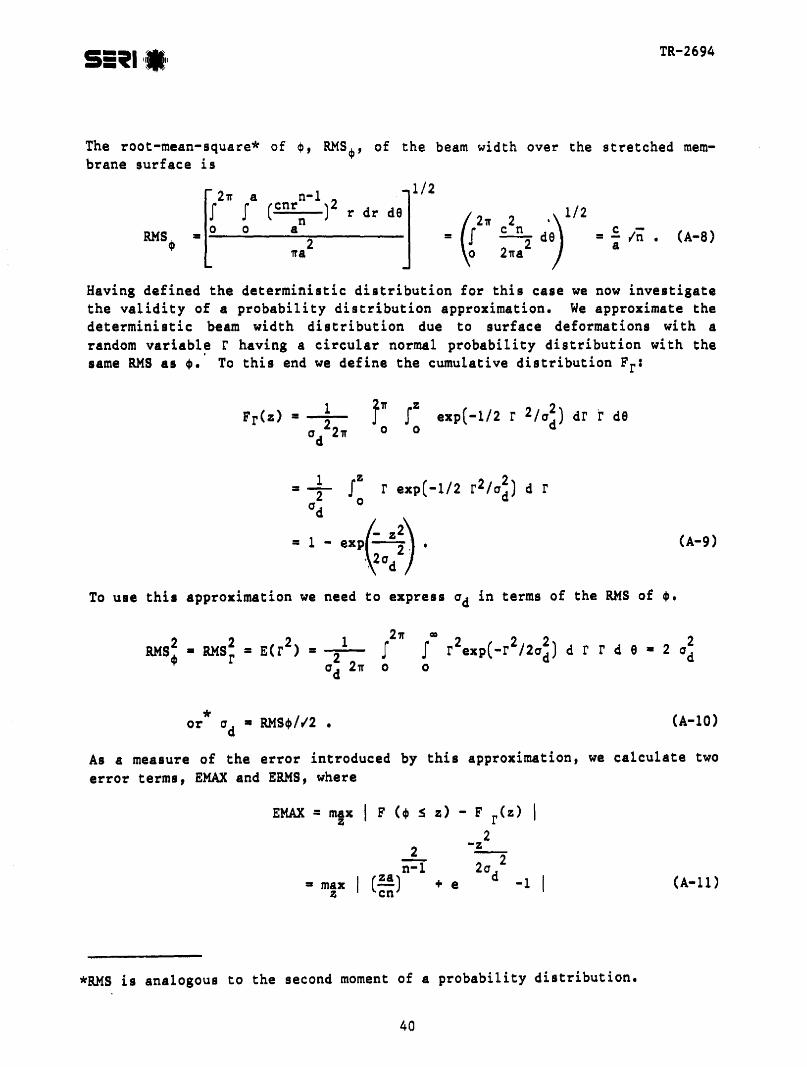
TR-2694

The root-mean-square* of ~, RMS~, of the beam width over the stretched mem­brane surface is

(

211' 2 ,)1/2J c n2 de = s Ino 211'a a

(A-B)

Having defined the deterministic distribution for this case we now investigatethe validity of a probability distribution approximation. We approximate thedeterministic beam width distribution due to surface deformations with arandom variable r having a circular normal probability distribution with thesame RMS as ~.' To this end we define the cumulative distribution Fr :

Fr(z) = --- J: exp(-1/2 r 2Ia~) dr r de

=_

1__ JZ ( 2 2)r exp -1/2 r lad d r2 0

=:d_ exp(.- z~,\ .'\2ad :J

(A-9)

To use this approximation we need to express ad in terms of the RMS of ,.

Im

2 ( 2 2) 2r exp -r 12ad d r r d e = 2 ado

(A-lO)

As a measure of the error introduced by this approximation, we calculate twoerror terms, EMAX and ERMS, where

F (, :s z)

2n=r(.!!) + ecn

EMAX = maxZ

=maxZ

- F r(z)2-z

--22ad -1 (A-II)

*RMS is analogous to the second moment of a probability distribution.

40

TR-2694

and

(A-12)

= cnla,

Substituting x z into Eqs. A-11 and A-12 gives=-O'd

2 r x2

EMAX = max I(.!..)n-1 + e-r - 11x In

and 2[;2,J/n-l x+ e '2 -1

ERMS =0 12n

Thus when b = 0 the error introduced by the normal approximation is inde­pendent of the values of a and c.

Figure A-2 graphically presents the density functions and the cumulative dis­tribution functions for both the circular normal approximation and the deter­ministic distributions for n = 3. Figure A-2 shows that although the densityfunction of ~he approximation may be very dissimilar in shape to that of thedeterministic distribution when n =3, the cumulative distribution functionsare nonetheless very close. Figure A-3 compares the deterministic distri­bution functions for n = 2, 3, and 4. From Figures A-2 and A-3 it is apparentthat the circular normal probability distribution best approximates the n = 3case. This is corroborated by the results in Table A-l.

Case 2: b > 0, C = o (no asymmetric deformation)

As in the preceding case we begin by defining the deterministic distribution.For this case by Eq. A-3,

*If we express r in terms of Cartesian coordinates we have RMS2 = E (r2) =E (rx2 + ry2) = E (rx2) + E (ry2) = ax2 + 0' 2 r, but since r has a circular

normal di i but i d 2 !Therefore ad =lstrl utlon ax = ay an RMS r = 20'd • a = ayeX

lt1

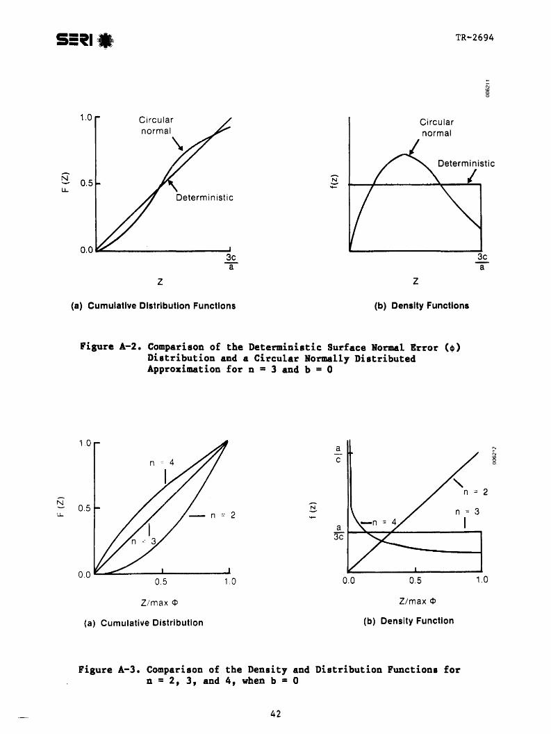
TR-2694

N<Coo

1.0

N""-' 0.5L1..

0.0 .....---------.....3ca

z

E-

Circularnormal

z

(a) Cumulative Distribution Functions (b) Density Functions

Figure A-2. Comparison of the Deterministic Surface Normal Error ($)Distribution and a Circular Normally DistributedApproximation for n = 3 and b = 0

1.00,50.01,00.50.0 ~~-----------

1,0 a '"- NC

<Ca0

= 2N

0,5 Eu, 2 n = 3

a I3c

Z/max ¢ Z/max ep

(a) Cumulative Distribution (b) Density Function

Figure A-3. Comparison of the Density and Distribution Functions forn =2, 3, and 4, when b = 0

42

Table A-i. Errors Introduced by theAssumption of a NormallyDistributed Surface NormalError when b = 0

n ERMS EMAX

2 0.098 0.153

3 0.055 0.087

4 0.104 0.198

TR-2694

(A-13)

Given our earlier definition of F(~ ~ z), we have

F(~ ~ z) = F (2 ~r ~ z) = F (r 5 Z2~2)a

= F r ~ h(z) ,

(A-14)

where

Thus h(z)Io

21Ta

r dr de

(A-lS)

The analog of the probability density function, f,(z}, is again found by dif­ferentiating F(, ~ z) with respect to z:

(A-16)

The root-mean-square, RMS, of the surface normal error over the stretched mem­brane surface is

RMS

(2b2r)2

r dr da21Ta

43

/2 b=--a (A-17)

TR-2694

The distribution of ~ in this case has the same form as the case consideredearlier in which b = 0 and n = 2 (compare Eqs. A-6 and A-lS as well asFigures A-3 and A-4 for n = 2). Therefore the errors ERMS and EMAX introducedby the circular normal probability distribution approximation are independentof both a and b and are equal to 0.097 and 0.153, respectively. These largeerrors are not surprising given the difference in the density functions shownin Figure A-4b.

Case 3: b > 0, C > 0 (both axisymmetric and asymmetric deformation exist)

As in the previous two cases we begin by defining the deterministic distri­bution. Let Fr(, S z) denote the fraction of the time that, is less than orequal to z on a circle of radius r centered at the center of the circularheliostat. By solving Eq. A-3 for 9 in terms of " we can express Fr (, S z)in terms of 9.

(A-lS)

NLL

1.0

z

(a) Cumulative distribution

N-

a-b

z

(b) Density function

2ba

Figure A-4. ComparisoD of the Deterministic Surface Normal Error (,)Distribution and a Circular Normally Distributed Approxi­mation for c = 0

44

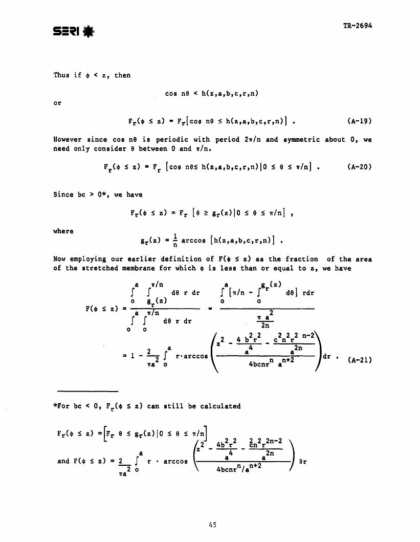
TR-2694

Thus if ~ < z, then

cos nB < h(z,a,b,c,r,n)or

Fr(, S z) = Fr[cos nB S h(z,a,b,c,r,n)] • (A-19)

However since cos nB is periodic with period 2w/n and symmetric about 0, weneed only consider 9 between 0 and win.

Fr(, S z) =Fr [cos nBS h(z,a,b,c,r,n)IO S 9 S wIn] •

Since bc > 0*, we have

(A-20)

wheregr(Z) =1 arccos [h(z,a,b,c,r,n)] •

n

Now employing our earlier definition of F(, S z) as the fraction of the areaof the stretched membrane for which, is less than or equal to z, we have

a win a g (z)J J dB r dr J [wIn - I r dB] rdr0 g (z) 0 0

FC, S z) = rwIn =a 2

J J dB r dr 'If a2n

0 0

r.arccos ~24 b

22 2 2 2 n-

2:lr c n r

-~Ia - 4 - 2n

= 1 a a dr4b n n+2 (A-2l)wa 0 enr a

*For bc < 0, FrC, S z) can still be calculated

Fr(, S z) = [Fr B S gr (a) los B S win]~2 _ 4b2r2 _ ~n2r2n-2

) 3ra 4 2n

and F(, S z) =_2 J r • arccos a a4b nl n+22 0 cnr awa

45

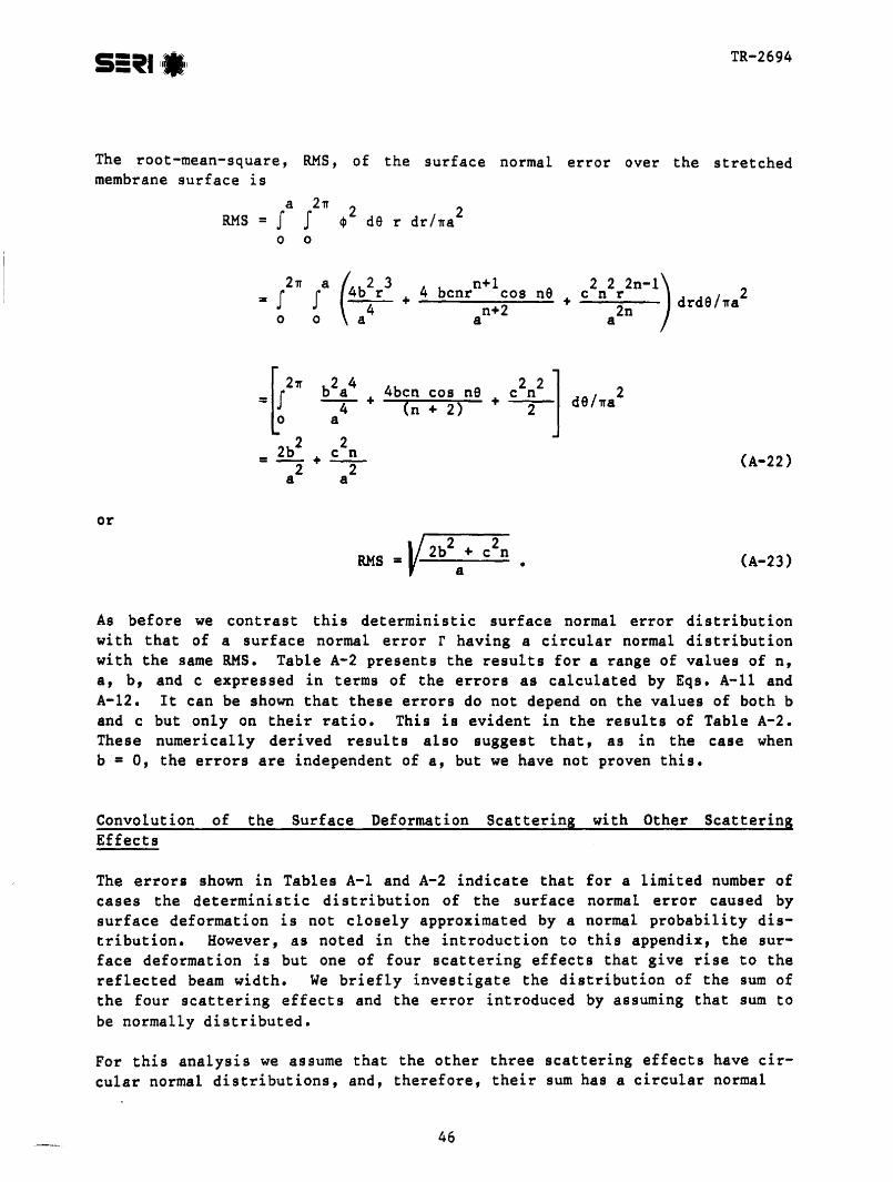
TR-2694

The root-mean-square, RMS, of the surface normal error over the stretchedmembrane surface is

a 21T 2 2RMS= J J 4» de r dr/1Ta0 0

21T a(-4::r

3+ 4

bcnrn+1 2 2 2n-l)= J J cos n6 + c na;n drd6/wa2n+20 0 a

[ 2w b2 4 4bcn cos ne 2 2 ]= J __a_ ++ c ~ de/1Ta24 (n + 2)

0 a

2b2 2c n (A-22)=-- + -2-2a a

or

=V- 2b2

a+2

RMSc n (A-23)

As before we contrast this deterministic surface normal error distributionwith that of a surface normal error r having a circular normal distributionwith the same RMS. Table A-2 presents the results for a range of values of n,a, b, and c expressed in terms of the errors as calculated by Eqs. A-ll andA-12. It can be shown that these errors do not depend on the values of both band c but only on their ratio. This is evident in the results of Table A-2.These numerically derived results also suggest that, as in the case whenb =0, the errors are independent of a, but we have not proven this.

Convolution of the Surface Deformation Scattering with Other ScatteringEffects

The errors shown in Tables A-l and A-2 indicate that for a limited number ofcases the deterministic distribution of the surface normal error caused bysurface deformation is not closely approximated by a normal probability dis­tribution. However, as noted in the introduction to this appendix, the sur­face deformation is but one of four scattering effects that give rise to thereflected beam width. We briefly investigate the distribution of the sum ofthe four scattering effects and the error introduced by assuming that sum tobe normally distributed.

For this analysis we assume that the other three scattering effects have cir­cular normal distributions, and, therefore, their sum has a circular normal

46

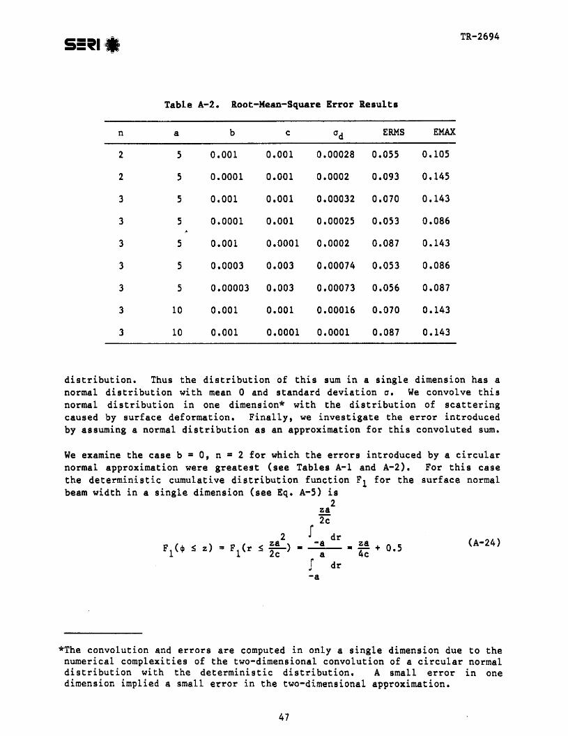
Table A-2. Root-Mean-Square Error Results

n a b c ad ERMS EMAX

2 5 0.001 0.001 0.00028 0.055 0.105

2 5 0.0001 0.001 0.0002 0.093 0.145

3 5 0.001 0.001 0.00032 0.070 0.143

3 5 0.0001 0.001 0.00025 0.053 0.086

3 5 0.001 0.0001 0.0002 0.087 0.143

3 5 0.0003 0.003 0.00074 0.053 0.086

3 5 0.00003 0.003 0.00073 0.056 0.087

3 10 0.001 0.001 0.00016 0.070 0.143

3 10 0.001 0.0001 0.0001 0.087 0.143

TR-2694

distribution. Thus the distribution of this sum in a single dimension has anormal distribution with mean 0 and standard deviation a. We convolve thisnormal distribution in one dimension* with the distribution of scatteringcaused by surface deformation. Finally, we investigate the error introducedby assuming a normal distribution as an approximation for this convoluted sum.

We examine the case b = 0, n = 2 for which the errors introduced by a circularnormal approximation were greatest (see Tables A-1 and A-2). For thi seasethe deterministic cumulative distribution function F1 for the surface normalbeam width in a single dimension (see Eq. A-5) is

2za2c

2 I drF

1( lj) S z) = F1(r < !!....) = -a = !! + 0.5 (A-24)

- 2c a 4cJ dr-a

*The convolution and errors are computed in only a single dimension due to thenumerical complexities of the two-dimensional convolution of a circular normaldistribution with the deterministic distribution. A small error in onedimension implied a small error in the two-dimensional approximation.

47

TR-2694

and the corresponding density function is

(A-25)

Since the scattering error introduced by surface deformation of a reflectingsurface is approximately twice the size of the surface norma1

2err~r, the

maximum scattering effect caused by surface deformation is 2 x -£ =.-£ anda athe corresponding density function is

a _ ax - - - •4c 8c (A-26)

Convoluting this density with that of a normal distribution with mean 0 andstandard deviation a yields the single dimension density function, h(y), ofthe sum:

hey) •

4c2"I _1 e

-4c al21f

2

2(y-z)

202!- dz •Bc (A-27)

The probability that the scattering beam width is less than x is found fromthe cumulative distribution function:

-x

.!... + 4co aa

Hex) =Ix

hey) dy =~ I4c x

a4caa

N(v) dv - 1 , (A-28)

where N(v) is the cumulative normal distribution function with mean 0 andsTandard deviation of one. The standard deviation of this convoluted sum,ar ef1' is

, (16C2 2)1/2ar ef1 = 3a2 + a (A-29)

We can now compare the distribution of this convoluted sum ~ith a normallydistributed approximation with mean 0 and standard deviation aref1. Table A-3shows the errors introduced by the normal approximation for several values ofa, c, and a. Although the error term, EHAX, was calculated using Eq. A-II, itshould be noted that this error is not strictly comparable to those calculatedearlier because it is measured in only a single dimension. Nonetheless, asshown by the results in Table A-3, convolution with a normal distribution witha ~ c significantly dampens any errors introduced by a normal approximationfor the scattering effects caused by surface deformation.

48

Table A-3. Error Introduced in a SingleDimension by a Normal Approx-imation when b = 0, D = 2

a c a EMAX

5 0.001 0.001 <0.015 0.001 0.0005 0.0155 0.001 0.0001 0.103

10 0.001 0.001 <0.0110 0.001 0.0001 0.0765 0.002 0.001 0.015

TR-2694

Conclusions

A circular normal approximation for the deterministic distribution of surfacedeformation scattering effects can be in error by a significant amount forsome cases. However, when the surface deformation scattering effects areadded to the scattering effects caused by the mirror material, trackingerrors, and concentrator size cone, the error introduced by the normal approx­imation is considerably dampened.

49

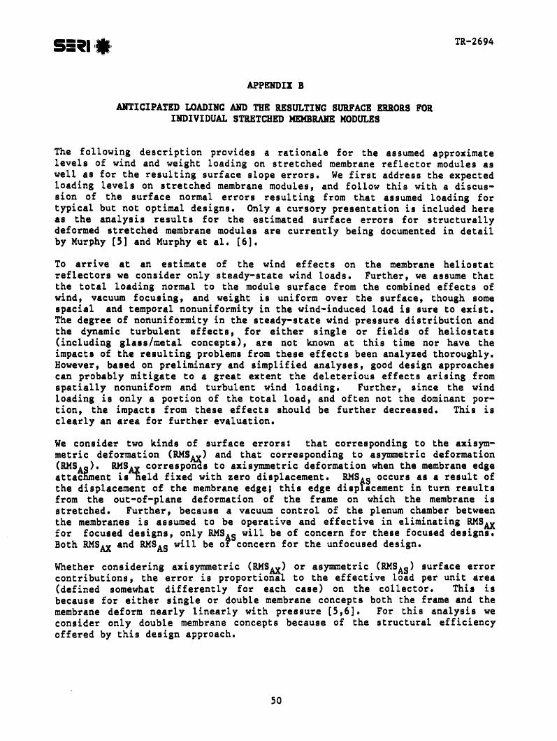
TR-2694

APPENDIX B

ANTICIPATED LOADING AND THE RESULTING SURFACE Buoas FORIllDIVIDUAL STRETCHED MEMBRANE MODULES

The following description provides a rationale for the assumed approximatelevels of wind and weight loading on stretched membrane reflector modules aswell as for the resulting surface slope errors. We first address the expectedloading levels on stretched membrane modules, and follow this with a discus­sion of the surface normal errors resul t ing from that assumed loading fortypical but not optimal designs. Only a cursory presentation is included hereas the analysis results for the estimated surface errors for structurallydeformed stretched membrane modules are currently being documented in detailby Murphy [5] and Murphy et ale [6].

To arrive at an estimate of the wind effects on the membrane heliostatreflectors we consider only steady-state wind loads. Further, we assume thatthe total loading normal to the module surface from the combined effects ofwind, vacuum focusing, and weight is uniform over the surface, though somespacial and temporal nonuniformity in the wind-induced load is sure to exist.The degree of nonuniformity in the steady-state wind pressure distribution andthe dYnamic turbulent effects, for either single or fields of heliostats(including glass/metal concepts), are not known at this time nor have theimpacts of the resulting problems from these effects been analyzed thoroughly.However, based on preliminary and simplified analyses, good design approachescan probably mitigate to a great extent the deleterious effects arising fromspatially nonuniform and turbulent wind loading. Further, since the windloading is only a portion of the total load, and often not the dominant por­tion, the impacts from these effects should be further decreased. This isclearly an area for further evaluation.

We consider two kinds of surface errors: that corresponding to the axisym­metric deformation (RMSAX) and that corresponding to asymmetric deformation(RMSAS). RMSAX corresponds to axisymmetric deformation when the membrane edgeattacnment isneld fixed with zero displacement. RMSAS occurs as a result ofthe displacement of the membrane edge; this edge dispracement in turn resultsfrom the out-of-plane deformation of the frame on which the membrane isstretched. Further, because a vacuum control of the plenum chamber betweenthe membranes is assumed to be operative and effective in eliminating RMSAXfor focused designs, only RMSAS will be of concern for these focused designs.Both RMSAX and RMSAS will be of concern for the unfocused design.

Whether considering axisymmetric (RMSAX) or asymmetric (RMSAS) surface errorcontributions, the error is proportional to the effective load per unit area(defined somewhat differently for each case) on the collector. This isbecause for either single or double membrane concepts both the frame and themembrane deform nearly linearly with pressure [5,6]. For this analysis weconsider only double membrane concepts because of the structural efficiencyoffered by this design approach.

50

TR-2694

For the axisymmetric contribution, the expression for the root mean squaresurface error RMSAX in terms of the load per unit aperture area of collectorPAX' is given, from simple linear membrane deformation analysis, by theapproximation*

(8-1)

where C1 is defined by

(B-2)

To is the total tension load on frame applied by the two membranes (each isassumed to have the same tension).

PAX is described as

1PAX = Wm cos ez + 2 (PNW) (B-3)

where PNW' the wind-induced pressure normal to the surface, is approximated by

(B-4)

W is the weight/area of the front reflector membrane and a is the radius oft~e membrane. CN is the loading coefficient which we have assumed to be 1.0.For a single isolated heliostat the value of CN may be as high as 1.5, but forfields of heliostats recent data indicate that Cu may be considerably below1.0. q is defined as the dynamic wind pressure (= 1/2 p2). e is the col­lector zenith angle as' shown in Figure B-1. The expression for) (and P S'which is defined below) assumes that the wind angle of attack isAfhe compte­ment of the 'collector zenith angle ez" but not the yaw angle (rotation aboutthe vertical axis in Figure B-1), which is assumed to be zero.

PAX is composed of two contributions, the weight on the reflector membrane,and that caused by the wind velocity induced pressure on the reflector sur­face. Two points are worthy of note. First, only the reflector membrane isconsidered in the weight contribution since only the reflector is of concernin the axisymmetric contributions (we do not really care how the rear membranedistorts). Second, the total pressure load on the collector caused by wind isassumed to be made up of two contributions of equal magnitude; i.e., apositive increase on the windward side of the collector and a negative

*This approximation is valid whether the displacement increment is measuredfrom an initially curved shape or from an initially flat condition. For theunfocused heliostats we will be returning to deviations from the flatcondition and will actually be penalizing the system for a benefit whichresults from gravity focusing.

51

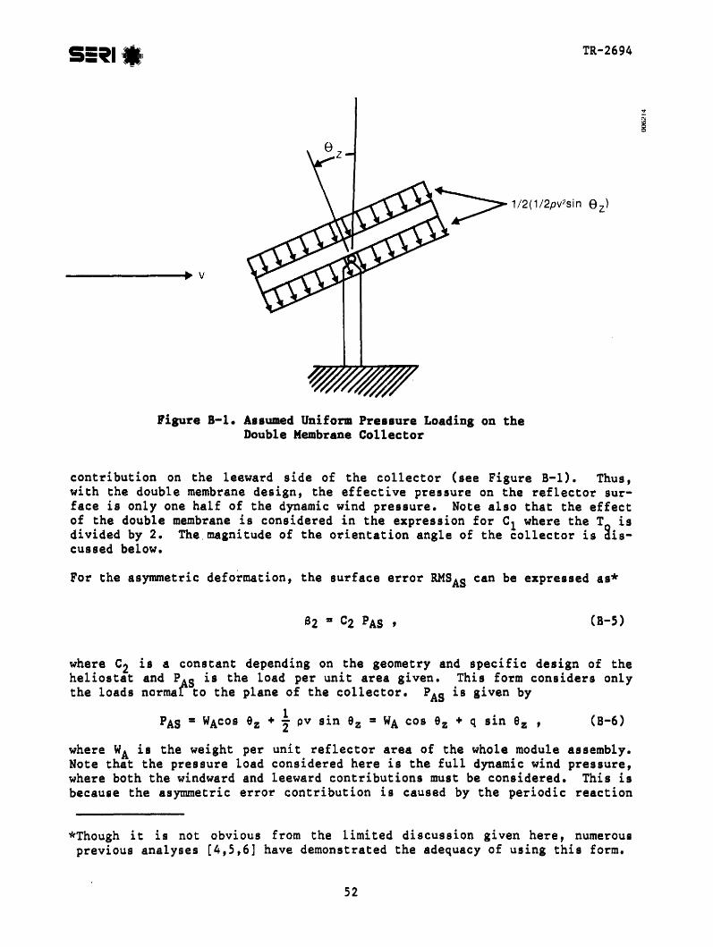
--------..... v

TR-2694

Figure 8-1. Assumed Uniform Pressure Loadinl on theDouble Membrane Collector

contribution on the leeward side of the collector (see Figure 8-1). Thus,with the double membrane design, the effective pressure on the reflector sur­face is only one half of the dynamic wind pressure. Note also that the effectof the double membrane is considered in the expression for Cl where the T isdivided by 2. The magnitude of the orientation angle of the collector is ais­cussed below.

For the asymmetric deformation, the surface error RMSAS can be expressed as*

(8-5)

where C2 is a constant depending on the geometry and specific design of theheliostat and PAS is the load per unit area given. This form considers onlythe loads normal to the plane of the collector. PAS is given by

PAS = WAcOS ez + t pv sin ez = WA cos ez + q sin 9z , (8-6)

where WA is the weight per unit reflector area of the whole module assembly.Note that the pressure load considered here is the full dYnamic wind pressure,where both the windward and leeward contributions must be considered. This isbecause the asymmetric error contribution is caused by the periodic reaction

*Though it is not obvious from the limited discussion given here, numerousprevious analyses [4,5,6] have demonstrated the adequacy of using this form.

52

TR-2694

forces, which must oppose the entire wind and weight load normal to the planeof the reflector.

A value for the wind-induced pressure must be determined. One measure forthat quantity, which is used in this analysis, is the expected value of thewind-induced pressure; i.e., the dynamic pressure weighted average of the windprobability distribution. Such wind probability distributions are availablefor selected locations [17,18] from previous studies. In these studies, thetotal amount of insolation corresponding to a specified velocity interval isgiven, and so the probability density of insolation as function of velocity,f(v), can be determined.* Then the expected value of the wind induced pres­sure q can be determined from

q = .!. p2

JClQ v2 f(v)dv =o

1 p v22" (B-7)

where it is assumed that the air density p is constant (i.e., not dependent onthe velocity v at the site).

Thus, for a given value of collector attitude, the expected values of PAX andPAS can be determined by

PAX JClQ PAX f(v)dv WM cos 9z + 1 - sin 9z= = - q0 2

and

PAS = JCD PAS f(v)dv = WA cos 8z+ q sin 8z .a

(B-8)

(B-9)

q is easily evaluated with Eq. B-7 along with the field data from McDonnellDouglas [18]. The results of this evaluation along with some other informa­tive statistics are given in Table B-1 for several locations and a "strawman"composite site, which is synthesized by averaging the insolation density func­tions for the seven sites considered in the study [18].

It is interesting to note from Table 8-1 that when using (v 2)1/2 as the mea­sure of velocity in the cumulative distributions, nominally 70% of the insola­tion at a given location occurs at or below this velocity whereas using theaverage velocity v the respective insolation level is approximately 60%.

RMSa and RMSAS can now be determined for a particular design using the abovedeflnition of q along with Eqs , B-7 and 8-8, known weight properties of themodule, and a given angle of attack.

PAX is shown a9 a function of 8 for Barstow for several membrane designs inFlgure B-2. At low angles of attack (9 small), weight is the primary contri­bution to PAX' while for large values (8 near 900

) , PAX is primarily due to

*Another description for f(v)dv is the fraction of solar energy that occursfor wind velocities in. the range of v and v + dv.

53

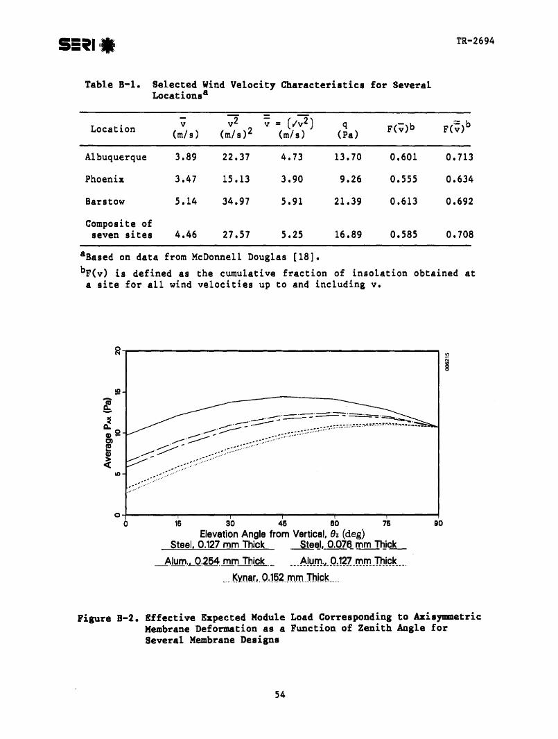
55'1 1

•

1TR-2694

Table 8-1. Selected Wind Velocity Characteristics for SeveralLocationsa

Location v y2 y = (/v2) q F(v)b F(~)b(m/s) (m/s)2 (m/s) (Pa)

Albuquerque 3.89 22.37 4.73 13.70 0.601 0.713

Phoenix 3.47 15.13 3.90 9.26 0.555 0.634

Barstow 5.14 34.97 5.91 21.39 0.613 0.692

Composite ofseven sites 4.46 27.57 5.25 16.89 0.585 0.708

aBased on data from McDonnell Douglas [18].

bF(v) is defined as the cumulative fraction of insolation obtained ata site for all wind velocities up to and including v.

~"""'-------------------------ltl~

9016 30 46 80 76Elevation Angle from Vertical, 9z (deg)

Steel, 0.127 mm Thick Ste~, O.076_mm 11Jj~

~lurn.~ ..264 ml1l Thick ._ ___~!I:IJn..I_QJ~Z_mm_ThlQ~ ....."Kyn.~r,.. ,Q~19.~ ...mm..TbJqk.... ,.

O-f-----r----~----r__---..,....--- ......---.....jo

Figure 8-2. Effective Expected Module Load Corresponding to AxisymmetricMembrane Deformation as a Function of Zenith Angle forSeveral Membrane Designs

54

TR-2694

wind pressure loading. It is noted that the wind-induced pressure on thereflector membrane is only one half of the expected value of the dynamic windpressure at the Barstow site since the module is a two membrane design. Fordesigns with heavy membranes (i.e" thick steel concepts), the weight will bethe dominant factor in determining the effective load for a wide range ofangles of attack. On the other hand, if the membrane is thin or of a light­weight material, such as aluminum or polymer, then the effective load will bedominated by the wind effect. In fact, a reasonable design pressure limit for"good" unfocused designs would appear to be the effective pressure load corre­sponding to the wind only.

Fig~re B-3 shows the RMS axisymmetric error contribution, RMSAX, as a functionof PAX for several module designs. Here it is seen that once the effectiveload is determined, the RMS error depends only on the membrane module radiusgeometry and tension level. If we use as the measure of effective pressureload, the value corresponding to wind only effects, then a reasonable upperlevel of error for RMSAX, corresponding to "good" design, is about 2 mrad forthe Barstow location. From the data in Table B-1 it is seen that for theother locations and for the "composite" site the corresponding level will besomewhat lower. Further, for advanced designs there may be the potential todesign for error levels that are considerably lower than the 2 mrad.

The situation for the !asymmetric load contribution PAS is considerably dif­ferent than that for PAX since the weight of module, though very low whencompared to glass/metal concepts, will in general be considerably greater than

...

.. " ..- .. .......

Cl ........I::,,;~-----T""------__........_----...,.------......fo 5 10 15 20

Average P.u (Pa)Rad. • 5 m. T. • 8750 N/m ~d~~_m~_· 8759 N/m_

---.R.ad..~.L~...!-T.L-~--2500~/m._ ___R~_d.! __~ __~ __~h __I! __~_JZ.~_Q.Q_J~!-,!,-

.. , ).Q.l7. p..~ ,~., w!.I1.q q.!:'J.y ,1.~.~.g .

Figure B-3. Effective RMS Surface Error as a Function of PAX for SeveralModel Designs

55

TR-2694

the reflector membrane only. Typical steel module designs with areal weightsof around 100 Pa (2.09 lb/ft 2) have been configured, while reflector membraneswell below 20 Pa (0.42 lb/ft 2) appear feasible. Figure B-4 illustrates thesepoints where the expected areal load for the module, corresponding to asym­metric deformation, is shown as a function of collector elevation angle forseveral assumed mod~le weight s (15, 100, and 125 Pa corresponding to 1.51,2.09, and 2.61 lb/ft). The lowest curve for 33 Pa shown in Figure B-4 corre­sponds to an aluminum design that is similar in construction to the 100-Pasteel designs. The weight is clearly the dominant factor for all of thesecases corresponding to the Barstow wind data. Hence, this led us to select areasonable lower limit of 300 for the zenith angle for the asymmetric loaddesign criteria (this will tend to result in conservatively high weightloads).

In making the surface error structural analysis comgutations corresponding tothe asymmetric error effects, a zenith angle of 30 (cos 300 = 0.81) and anapplied pressure of 10 Pa (corresponding to a mean dynamic pressureof - pv =10/sin230 =20 Pa at ez =300 ) were selected. It was felt that thiscom~ination represented a reasonable average total load corresponding to asym­metric deformation •

• ~'~'-="'""'-=-'~'-_.~=~. ~~--=-- ~.-- ..............---.-- -......... ....'-- .............. '

'--. "<,............... ....'- '".........................

....................................................................... ~~::::~..

0+----....,.----....,------,.----.,.....---.....,.-----1o 16 30 46 60 76, 90

Elevation Angle from Vertical, 8z (deg)Steel Design. Wit. - 126 Pa Ste~ Desigl}, Wit. -_ 100 Pa__

j.teel. De.1Qn. W~~£§..P.L. . __A!IJJn.._O_Q'jQ."L_~~_~ __3_~.P.'. __

Figure 8-4. Average Load Corresponding to Asymmetric Loadingfor Several Model Designs

56

S=!!!SI !l.~~!-~'-~

TR-2694

The asymmetric error level associated with these assumed loads (seeFigure B-5) is described next. The results illustrated in Figures B-7 throughB-I0 show typical structural analysis results as calculated with the NASTRANfinite element method [19] and with a more simple analytical approach asdescribed in [5]. The phenomena leading to these results are described muchmore extensively in Murphy et ale [5] and Murphy [6]. Furthermore, theresults demonstrate that these load induced error levels can potentially becontrolled to quite low levels. The modules considered are shown inFigure B-6; i.e., steel construction, 5-m radius, O.254-mm-thick membranes,2h x 76.0-mm frames with 3.048-mm-thick walls. Figure B-7 shows how thebending and torsional rigidity vary with frame height for the selected framedesign.

Figure B-8 illustrates for several module designs how the peak frame deflec­tion (midway between the supports) varies as a function of frame height forthe assumed loading on the module. The curve with the highest deformationcorresponds to a single membrane design, and the next lower curve correspondsto a double membrane design with attachments that can slide circumferentiallybut not radially. The lowest overall deflection curve corresponds to a doublemembrane design with hard at tachments (bounds or welds) to the frame. Themechanics of why these modules behave so differently will not be discussedhere (see Murphy et ale [6]). However, it is clearly seen that module perfor­mance can be dramatically improved with different design approaches, and very

10 PA

Figure 8-5. Effective Expected Module Area Load Corresponding to AsymmetricDeformation as a Function of Zenith Angle for Several ModuleWeights

57

(a) Perspective view - stretched-membrane reflective module;pin supported at three equidistant circumferential points

W

2W

R ': 5.0 ma 4,96 m2W - 76,2 mm

(b) Top view - stretched-membrane reflective module

TR-2694

Single-membrane design

l'2h

(Viall th ickness= 3.048 mm

Double-membrane design

(c) Cross-section view for steel frame/membranecombination considered In analysis discussion

Figure 8-6. Esample of Module Construction

58

TR-2694

small deformation limitations appear possible. The way in which these defor­mations translate into surface errors is seen in Figures B-9 and B-10, wherethe asymmetric error contribution (RMS~ ) for the three designs discussed inFigure B-7 are plotted as a function of irame half-heights (in Figure B-9) andthen as a function of total module areal weight (in Figure B-10). It is seenthat the asymmetric error, RMSAS' can potentially be controlled to better thanabout 0.5 mrad (rms) at a module areal weight of about 100 Pa for the steeldesign shown. It might also be noted that for aluminum designs the same errorlimitation appears attainable for about 1/3 the weight [6].

Based on these findings the macroscopic surface shape for the focusedstretched membrane modules appears to be potentially as good as that corre­sponding to the state-of-the-art glass/metal heliostats when only the asymme­tric error contribution is considered. More specifically our calculationsshow the potential to limit wind- and weight-induced deformations to about0.5 mrad rms total for the asymmetric portion, and this appears to be at leastas good as typical glass/metal designs. It is assumed that the axisymmetriccontribution caused by uniform pressure is negligible. However, the controlof the plenum chamber may fall significantly short of this goal when nonuni­form pressure loads are considered. This area remains a significant unknown.

On the other hand, the surface errors for the unfocused stretched membraneheliostats can potentially be larger because of the axisymmetric contributionwhich is not considered to exist in the focused controlled stretched membrane

2-------------------------------.(7)~

-0C'ol ltIe -.

IZ

ltI00-0--

270120 150 180 210 2~0

Half Height (mm)c Flexural EI ~9rllonal GK

90o .......---~~--~--- __---_---_---~-----'

60

Figure B-7. Torsional and Flezural Rigidity as a Functionof Frame Half Height

59

TR-2694

- S ...-------------------------___. !i::e N

~ 8

270

\ ,-,

'<; "-"-., ~

~'-- ----'-- ...'a--._. ~ - ---e-~-'-' --€I--......_._'"""A

90 120 150 180 210 2~0

Half Height (mrn)Cl Single Membrane ~9uble/_Radial Fix

_"'_. Do.ubl,L.Rac;lJ.g1.~.Clr~um.B~

e::INe';(e~o_+_--__,.---_,_--___,---_r_---~--....,...--___f

60

ee0'"..

LL.

CGO,2-u.s';-0o

Figure 8-8. Mazimum Frame Deflection as a Function of Frame Half Heightfor Several Construction Types

N..-----------------------------,~

..o....

w

euo-..::J

1nVJ oVJ

~AI!:

\o~

'" "~ ~............. ...'a.- ~'-- ... ---.--bt----._ 'El _

'-,'-.-::::::--=.. ~

27090 120 150 180 210 2.040

Half Height (mm)Cl Single Membrane ~9ublel_Radial Fix

_"'_..Q.g.ubl,L.Rac;lJ.g1.~.Clr~um.B~

o-+----.,.----or-----......r----.......,.---.....,..---""""I"""---460

Figure 8-9. RMS (Surface Averaged) Error as a Function of Frame Half Height.Asymmetric error portion. In double membrane designs theasixymmetric error portion is assumed to be eliminated.

60

TR-2694

\\

\\

\-, ~,

.')..-...... ....-....... ---........" ..~

--.--. - --e-~'-'-'--' - --"'€l'-.--.--ta

Itl

~-r-----------------------------,!,...."eL.-E

'-J

150100 125

Total Weight/Reflector Area (N/m2)

c Single Membrane ~guble {RadiaL Fix

_1>_. Do.ubl,-'Rac;fJ.g1 ..!....Clr~um.B~

O-+---------..,...---------.,..-----------t75

Figure 8-10. RMS (Surface Averaged) Error as a Function of Total ModuleWeight per Unit of Reflector Area. Asymmetric error portion.

concept. We have established a reasonable bound on these errors of about 2mrad rms total in addition to the surface errors corresponding to the glassmetal concepts. This bound is based on assumed good design practice and couldpotentially be less than this level, especially for smaller radius designs.Of course, it is possible to do considerably worse than this, by inappropriatedesign of the unfocused module. For example, low initial tension levels andheavy (thick) membranes can push the error dramatically beyond the 2.0 mradlevel if care is not exercised.

It should be' emphasized that neither the focused nor the unfocused designs areoptimal, but are rather "typical" in that it is known that a number ofimprovements relative to the design considered here are possible. Forinstance, the frame thickness assumed in the analysis presented by Figures B-7through 8-10 is believed to be too thick for optimal conditions, and more thanthree supports may be desirable from a cost/performance perspective.

One final note of importance is that in designing an unfocused module, theprocess is more complex than merely taking a focused module and leaving offthe controls and vacuuming subsystem. For instance, the desired operatingtension would be considerably higher than typically assumed by SNLL for theircontrolled modules. Second, the lighter and thinner membranes of the unfo­cused module are also much more desirable in terms of performance consider­ations. In addition, it appears that different tension levels in the frontand back membranes may be desirable (the higher tension being in the frontmembrane with the reflective surface on it). Further, different tensionlevels in the membranes need not mean unbalanced moments on the frame sincethe height above the frame torsional shear center might be varied to accountfor this.

61

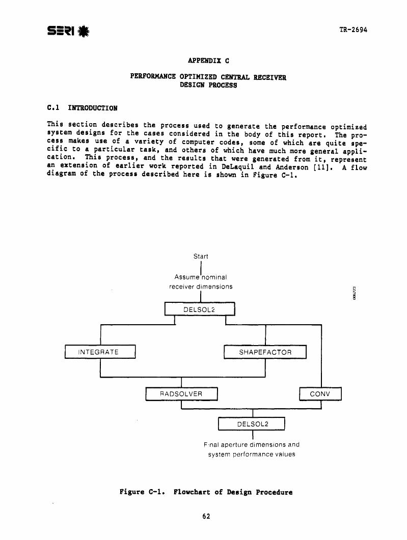
TR-2694

APPEllDIX C

PERFORMANCE OPTIMIZED CENTRAL RECEIVERDESIGH PROCESS

C.l I HTKODUCTIOR

This section describes the process used to generate the performance optimizedsystem designs for the cases considered in the body of this report. The pro­cess makes use of a variety of computer codes, some of which are quite spe­cific to a particular task, and others of which have much more general appli­cation. This process, and the results that were generated from it, representan extension of earlier work reported in DeLaqui1 and Anderson [11]. A flowdiagram of the process described here is shown in Figure C-l.

Start

AssumJnominalreceiver dimensions

INTEGRATE SHAPEFACTOR

Final aperture dimensions and

system performance values

Figure C-l. Flowchart of Desigo Procedure

62

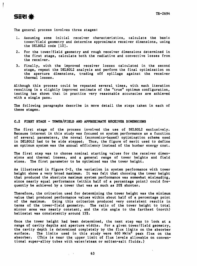
TR-2694

The general process involves three stages:

1. Assuming some initial receiver characteristics, calculate the basictower/field geometry and determine approximate receiver dimensions, usingthe DELSOL2 code [10].

2. For the tower/field geometry and rough receiver dimensions determined inthe first stage, calculate both the radiative and convective losses fromthe receiver.

3. Finally, with the improved receiver losses calculated in the secondstage, repeat the DELSOL2 analysis and perform the final optimization onthe aperture dimensions, trading off spillage against the receiverthermal losses.

Although this process could be repeated several times, with each iterationresulting in a slightly improved estimate of the "true" optimum configuration,testing has shown that in practice very reasonable accuracies are achievedwith a single pass.

The following paragraphs describe in more detail the steps taken in each ofthese stages.

C.2 FIRST STAGE - TOWER/FIELD AND APPROXIMATE RECEIVER DIMEHSIOHS

The first stage of the process involved the use of DELSOL2 exclusively.Because interest in this study was focused on system performance as a functionof several parameters, the normal (economics-based) optimization scheme usedin DELSOL2 had to be side stepped. Thus, the figure of merit used to definean optimum system was the annual efficiency instead of the busbar energy cost.

The first step was to choose nominal starting values for the receiver dimen­sions and thermal losses, and a general range of tower heights and fieldsizes. The first parameter to be optimized was the tower height.

As illustrated in Figure C-2, the variation in system performance with towerheight shows a very broad maximum. It was felt that choosing the tower heightthat produced the absolute maximum system performance was somewhat misleading,since nearly equal performance (within half of a percentage point) could fre­quently be achieved by a tower that was as much as 20% sho~ter.

Therefore, the criterion used for determining the tower height was the mlnlmumvalue that produced performance values within about half of a percentage pointof the maximum. Using this criterion produced very consistent results interms of the tower-field geometry. The ratio of the tower height to totalmirror area was nearly constant, and the rim angle to the farthest (north)heliostat was consistently around 15%.

Once the tower height had been determined, the next step was to look at arange of cavity depths and aperture widths. For a given tower/field geometry,the cavity depth is determined completely by the flux li~its on the absorbersurface. The limits used in this study were 600 MW/m peak flux on theabsorber. (This is near the upper limit of flux levels allowable on conven­tional super-alloy tubes with water/steam or molten-salt fluids.>

63

TR-2694

....c-----------------------------. ~~

~>-,0 -ue.!.~-It'\- .we

3S0I

2S0Tower Height em)

200lS0

CO!

e ........------~-----......,------__r-------I

Figure C-2. Variation of System Performance with Tower Height

The aperture dimensions are determined by trading off spillage (the amount ofradiation incident upon the aperture plane that does not pass through theaperture) against thermal (both radiative and convective) losses from thereceiver. As the aperture dimensions increase for a given receiver, the spil­lage will decrease and the thermal losses will increase.

Obviously, the outcome of this tradeoff depends on a number of factors,including receiver parameters such as geometry and operating temperature, aswell as field characteristics such as focusing and canting of the heliostatsand the size and shape of the field (both of which influence the compositeimage).

DELSOL2 optimizes the aperture dimensions by scaling the receiver thermallosses directly with the aperture area. Since in this first stage of thedesign process only approximate values of the losses are available, the heightand width of the aperture are not varied independently, but rather the ratioof the height to the width is held constant and the losses and spillage arecalculated for a range of aperture sizes.

Once the approximate aperture dimensions have been determined, DELSOL2 hasenough information to produce a Itmaplt of the flux levels on the absorber wall.Then the receiver depth and height, the approximate aperture dimensions, andthe absorber flux map can be passed to the second stage of the design process.

64

rTR-2694

C.3 SECOND STAGE - RECEIVER LOSSES

The second stage of the design process involves calculating the receiverlo~ses for the cavity geometry and aperture dimensions that were determined inthe first stage. This calculation takes place in two parts: the radiativelosses (both reflected and emitted) are calculated, and then the convectivelosses are calculated.

An isometric view of the receiver used in this study is shown in Figure C-3a.To calculate the radiative losses, the interior of the receiver is dividedinto a number of zones, each of which acts as an independent surface inreceiving and emitting radiation. Although most of the inactive surfaces inthe receiver are modeled with a single zone per wall, the absorber surface wassubdivided into a number (on the order of 20 to 30) of smaller zones, as shownin Figure C-3b, because of the variation in the solar flux levels on it.

The ultimate calculation of the radiative losses is done by a program calledRADSOLVER [12], which was also written at Sandia National Laboratories,Livermore. RADSOLVER requires three sets of information to do itscalculations:

1. The incoming solar flux profiles as calculated by DELSOL2

2. A description of the geometry of the receiver, in the form of a table ofshape (or configuration) factors and the surface areas for each zone

3. The boundary conditions of the zones within the receiver (i.e., the tem­perature of--or heat flux through--that surface).

The values reported in the flux map output by DELSOL2 are local values calcu­lated for a matrix of points on the absorber surface. For RADSOLVER to usethem, this matrix of point values must be integrated and averaged over each ofthe zones in the radiative model. This is accomplished in a program that com­putes the double integral over each of the zone using a bicubic spline inter­polant to "fit" the matrix of point values from DELSOL2. These integratedvalues are averaged over the zones, and then output from the program alongwith the total flux incident on the absorber.

The tables of shape factors and zone areas are output from a program namedSHAPEFACTOR [131, which was originally developed at the University ofWashington. It uses a geometric description of the vertices (corners) of eachof the zones to assemble a model of the interior of the receiver and calculatehow much of the radiation leaving a particular zone will strike each of theother zones (i.e., the extent to which each zone can "see" each of the otherzones). It also calculates the areas of each of the zones.

In the terms used in this problem, the boundary condition information gen­erally describes whether the zone in question is an active (heat-absorbing)surface or an inactive one. Since the inactive surfaces are assumed to bewell insulated, with negligible conduction losses (since we are ignoring theinteraction between radiation and convection), they are described to the modelas adiabatic (zero net heat transfer). The active surfaces are, of course,

65

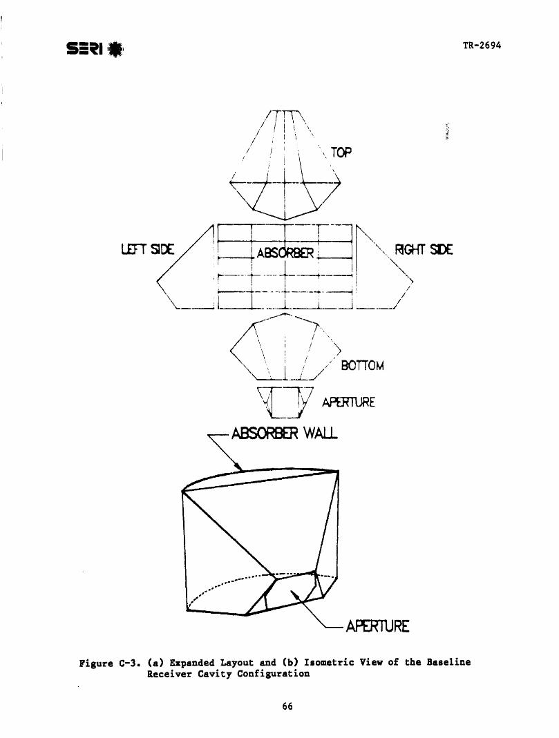
TR-2694

~]7 AffiffiJRE

~ ABSORBER WIill-

APERlURE

Figure C-3. (a) Expanded Layout and (b) Isometric View of the BaselineReceiver Cavity Configuration

66

,TR-2694

absorbing an as yet unknown amount of energy, so it is not possible to specifythe net heat flux through them. We do know, however, what temperature we wantthem to be operating at, and this provides the requisite boundary condition.

The other type of information that could loosely be classified as a boundarycondition and is required by the model is the hemispherical reflectivity ofeach of the zones. For the study reported here, the active surfaces weregiven a reflectivity of 0.1, while the inactive surfaces were assigned a valueof 0.4.

Once these three pieces of information have been gathered, they form the inputto RADSOLVER. Although RADSOLVER is capable of performing the radiativeexchange calculations on a number of spectral bands, the single-band or gray­body approximation was used. This is a cornmon "first order" approximation,which significantly reduces the required amount of calculational effort.Since the situation being modeled was quite generic, the minor loss of accu­racy associated with using this approximation was judged to be well within theuncertainty with which the multiband surface properties would be known.

The convective losses are calculated using a correlation proposed by Kraabeland Siebers [20] of Sandia National Laboratory. The correlation is:

where

h = (C-l)

h = the overall heat transfer coefficient based on the totalinterior of the cavity (W/m2 °C)

= the interior wall temperature (Oe)

= the ambient temperature (oe)

=the interior area of the cavity below the top of the aperture(including the floor)

the total interior area of the cavity.

The wall temperatures in Kraabel's tests were nearly isothermal. In a realreceiver, of course, there are significant variations in the wall temperaturesbetween surfaces, especially between the active surfaces and the inactive sur­faces. This situation is particularly acute for direct absorbtion receivers,where the absorbing fluid may be entering the top of the cavi ty 4000-5000C

colder than it leaves at the bottom. The approach taken here is to calculatean area-weighted average interior surface temperature based on the temper­atures calculated in the radiative model. This area-weighted average is thenused in Eq. e-1 to calculate the convective losses.

One drawback of the scheme used here for calculating the receiver losses isthat the convective and radiative losses are calculated independently.Although these two mechanisms are not truly independent, this approximation isquite good as long as the receiver loss fractions are reasonably small.

67

TR-2694

However, the procedure would lead to increasing overprediction of the lossesat high loss fractions.*

C.4 THIRD STAGE - APERTURE OPTIMIZATION AND PERFORMANCE ANALYSIS

The third stage of the analysis again uses DELSOL2. In this stage, the aper­ture dimensions are optimized. As before, a range of aperture dimensions istested, and the combination of width and height that produces the best annualsystem performance is chosen. This analysis is conducted with the other sys­tem parameters (e.g., field/tower geometry and cavity depth) that were deter­mined in the earlier analysis. Obviously, if the newly optimized aperturedimens ions are radically different from the originally as sumed values, thesecond stage should be repeated to determine better loss values. However, itis usually possible to choose the original dimensions close enough to thefinal ones so that such iteration is not necessary.

Finally, once the aperture dimensions for optimum performance have been deter­mined, a final DELSOL2 run is made to calculate a detailed summary of both thedesign point and the annual system performance.

*In order to correctly account for this interaction, it would be necessary tobe able to predict the convective losses from each wall individually. Thenthe convective and radiative losses could be calculated iteratively, aprocedure that would probably converge fairly quickly. Unfortunately, thereis no well-verified method now available for predicting convective lossesfrom individual surfaces in the complex flow situation found inside thereceiver. Additionally, the error associated with this approximation forsmall loss fractions is probably no worse than the inaccuracies associatedwith a number of the parameters or models used in the analysis. For thesereasons, the losses are calculated without including this interaction, andthis fact is simply noted.

68

TR-2694

(0-1)

APPENDIX D

PERFORMANCE OPTIMlZATIOH VERSUS COST/PERFORMANCE OPTIMIZATIOH

In the system analysis portion of this study, the system is designed solely onthe basis of performance. The optimum design 0 is assumed to be the one thatmeets the preselected annual delivered energy (E) and temperature requirementswith the highest efficiency; i.e., the design yielding the highest deliveredenergy per square meter of heliastat.

E EAc(D) =~x Ac(O) ,

where Ac(O) is the field area for design O.

In 'reality, the optimum design is the design that Mlnlmlzes system cost whilestill meeting the preselected delivered energy and temperature requirements.The system cost Cs comprises the costs of the individual components in thesystem.

(0-2)

where

Ca = the cost per square meter of heliostat

CT(h) = the cost of a tower of height h

Ca = the cost of the receiver

Cc • the cost of the controls

CBOS = sum of all additional costs necessary to deliver energy tothe base of the tower.

In selecting the optimal design three principal parameters are varied--thefield area, tower height, and receiver aperture size. Since the cost of con­trols and balance of system do not vary appreciably with any of these threeparameters, they need not be considered in a cost/performance optimization.Thus Eq. 0-2 can be reduced to

(0-3)

where K't is a constant cost and all other costs are a function of the designO.

Current knowledge of the sensitivity of the cost of a single cavity receiverto changes in the aperture size is extremely limited. Furthermore, our per­formance optimizations using DELSOL2 indicate that the optimum receiver con­figuration is insensitive to the characteristics of the different types ofheliostats that we examine in this study. Therefore in the cost/performanceoptimization the receiver cost can be considered to be a constant equal to thereceiver cost in the base case configuration, and Eq. D-3 reduces to

(0-4)

69

TR-2694

Earlier studies [21] have shown that tower cost CT is highly uncertain butsensitive to tower height. However, as shown in Figure C-2 of Appendix C,system performance is highly insensitive to tower height. Therefore for allpractical purposes the tower height can be assumed to be a constant, andEq. D-4 reduces to

(D-5)

Thus our cost/performance optimization has been reduced to the followingproblem:

(D-6)

subject to the constraint that E(D) = E where E(D) is the annual energydelivered to the base of the tower by design D. But this is equivalent tomaximizing the annual energy delivered per square meter of heliostat. Thusthe optimal design 0 is such that

(D-7)

and a cost/performance optimization yields the same optimal design and optimalsystem cost as the performance optimization performed in this study (compareEqs. D-l and D-7).

To arrive at this conclusion concerning the essential equivalence of a perfor­mance optimization and a cost/performance optimization, we made some simpli­fying assumptions concerning the cost of receivers and the performance sensi­tivity to tower height. We intend to examine these assumptions in the futureas more cost data become available.

70

TR-2694

APPEJiDIX B

SPECULARITY AIm COIlE SIZE IlELATIOHS

The analysis presented below provides a simple approximation for describingand relating specular reflectance, specular cone size and the total amount ofenergy reflected within that cone size.

As discussed by Pettit et ale [7,22,23,24], an incoming collimated beam oflight t is reflected from a reasonably good solar reflector not as a simpleperfectly specular beam but rather as scattered light about the nominalreflected ray defined as the specular direction 1 in a fairly narrow cone (seeFigure E-l). Further, it is shown that the intensity of the reflected beam,measured with respect to the specular direction, is proportional to the prod­uct of the total solar averaged hemispherical reflectance*, Ps' and a geo­metric factor G(!), which is a function of the half cone angle, !, measuredfrom the specular direction. Their data also shows that the scatter of thereflected light about the specular direction can often be accurately repre­sented by a normal or Gaussian probability distribution.

Surface normal

Incident ray

Specular direction

Half cone angle

Figure 1-1. Cone Containing Scattered Beam about the Specular Direction

*Averaged over the entire range of wave lengths in the solar spectrum.

71

TR-2694

If we assume that the distribution is a simple circular Gaussian* distribution

about the specular direction, then the fraction, p (V), of the incomingTS

radiation that is reflected within a cone about the specular direction, havinga half angle V, is given by

(E-l)**

G(V) is the cumulative distribution function corresponding to the circularGaussian distribution and is defined by

I (L )2V 2 - 1 2G(t) = 1 - e- 1/ 2 (;-) • 1- r2w rt -1- e a, d,dz , (E-2)

'I' 21T 6 6 2a,where a~ is the standard deviation of the half-cone angle'. With the abovedefinitlons G(t) can be interpreted as the ratio of the total specular reflec­tivity corresponding to a given cone angle size to the total hemisphericalreflectivity.

It is important to note that , is the half-cone angle whereas the data fromtests are typically given for a full-cone angle a (= 2'). This difference inconventions has evolved since analytical models usually employ probabilitydistributions in which the half-cone angle is the random variable, whereasmany two-dimensional experiments measure the energy within the full-coneangle.

Figure E-2 shows the fraction of energy (G) within a given half-cone angle asa function of ,Ia,. It is seen that for half-cone angles of , = 0 , 20 , and3a" the corresponding energies within the cone are about 40%, 901, and 99%,respectively. We can use Figure E-2 to determine, for given values of G('I')and " the corresponding value of o!' Alternately the standard deviation of ,can be determined by inverting Eq. E-2 to give

(1-3)***

(J

21-2 1n(1 - G('f»

'fa =--------- • ---------'f 1-2 In(l - G('f»

*The uniform circular Gaussian distribution assumes that distribution about thespecular direction l is axisymmetric, Nonaxisymmetric situations can be con­sidered if sufficient data are available [9],

**This form assumes that a single circular normal distribution is sufficient todescribe the scattering. Pettit describes cases in which two such distribu­tions are linearLy superimposed. In most cases, however, a single distribu­tion provides a very good approximation,

***This of course assumes that a single circular normal distribution adequatelydescribes the scattering.

72

TR-2694

32.520.5

o~d

eo;u.,Lto~.r;;::;.....-...,..---___,r__---...,......---"'""'T""---......,---___t

o

... -_.__------------------------=::====t ~

o ~

>0.0mit!L.OI»C

W

Figure B-2. Fraction of Reflected EnerlY in a Given Cone Size

The form of Eqs. E-l and E-2 can also be used to incorporate other beam broad­ening effects in addition to specularity in the calculation of the fraction,PTS C' ) , of the incoming radiation, which is reflected within a cone with halfangle ,. Let 9r ef l be the half-cone angle that includes not only specularitybut also n other beam broadening effects, 9k (k = 1, 2,--,n)

n

9r ef l =, + kb1 9k • (E-4)

If these other effects can be assumed to be independent and circular normallydistributed, then the distribution of 9 efl found by convolving the distri­butions of the different effects will afso be circular normally distributed.The standard deviation of 9r ef l in a sinlle dimension, 0refl' is then given by

n

(E-S)

2= Ps {i - exp[ -1/2 (+-) ]}

refl

Thus by Eq. E-2,

and by Eq. E-1,

G(9) =- 1 - exp2

[-1/2 ( 9 ) ] ,°refl

(E-6)

73

TR-2694

APPENDIX F

RECEIVER CONFIGURATION

One of the areas of central receiver design that seems the least developed isthat of the cavity receiver configuration*. Although the effect of the over­all configuration of the cavity on radiative losses is readily apparent, cur­rent evidence [19] indicates that the convective losses are also dependent onthe configuration, particularly on the amount of hot interior surface area andthe placement of the aperture.

The cavity configuration used to generate the results presented in the body ofthis report is shown in Figure C-3 in Appendix C. It was originally designedfor a study of high-temperature systems at fairly high flux levels [11].Although it performs quite well for this range of parameters, a major limita­tion of this design is that it can accommodate only a limited aperture widthbefore the inactive side walls begin to face outward through the apertureinstead of inward at the absorber.

Unfortunately, for some of the systems that used the larger sizes of unfocusedstretched membrane heliostats at the small plant size, the optimum aperturedimensions were larger than could be accommodated by this original config­uration. In these cases, the results presented in the body of the report weregenerated using the largest aperture possible with this configuration.

To establish how far off the optimum these results were, another configurationwas briefly investigated. An isometric of this new configuration is shown inFigure F-l. This new design allows much larger aperture sizes, but has somedisadvantages in terms of the amount of hot inactive surface area.

The results from this new configuration did show an improvement in performancefor .systems requi ring larle aperture areas. The resul t s are compared inFigure F-2 for the lOO-m unfocused stretched membrane heliostats at thebaseline surface errors (oopt = 3.46). The maximum difference is almost 10%at the lower temperature, while the difference nearly disappears at thehighest temperature. It appears from this data that there is a crossoverpoint somewhere; on one side of this point the original receiver configurationwill perform better, while on the other side the new design will be better.

*In this discussion, the cavity configuration refers to the overall geometry,including the shape of the absorber, the shape and angle of inclination of theaperture, and the geometry of the inactive surfaces that connect the apertureto the absorber. The particular dimensions of a configuration, including theheight and depth of the cavity and the aperture dimensions, are optimized foreach case considered. See Appendix C for a discussion of this optimizationprocess.

74

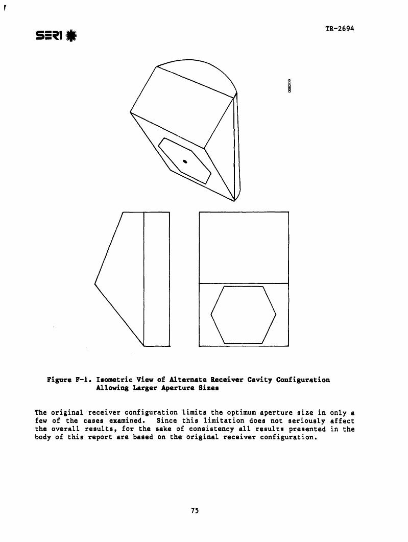
TR-2694

Figure r-l. Isometric View of Alternate Receiver Cavity ConfigurationAllowing Larger Aperture Sizes

The original receiver configuration limits the optimum aperture size in only afew of the cases examined. Since this limitation does not seriously affectthe overall results, for the sake of consistency all results presented in thebody of this report are based on the original receiver configuration.

75

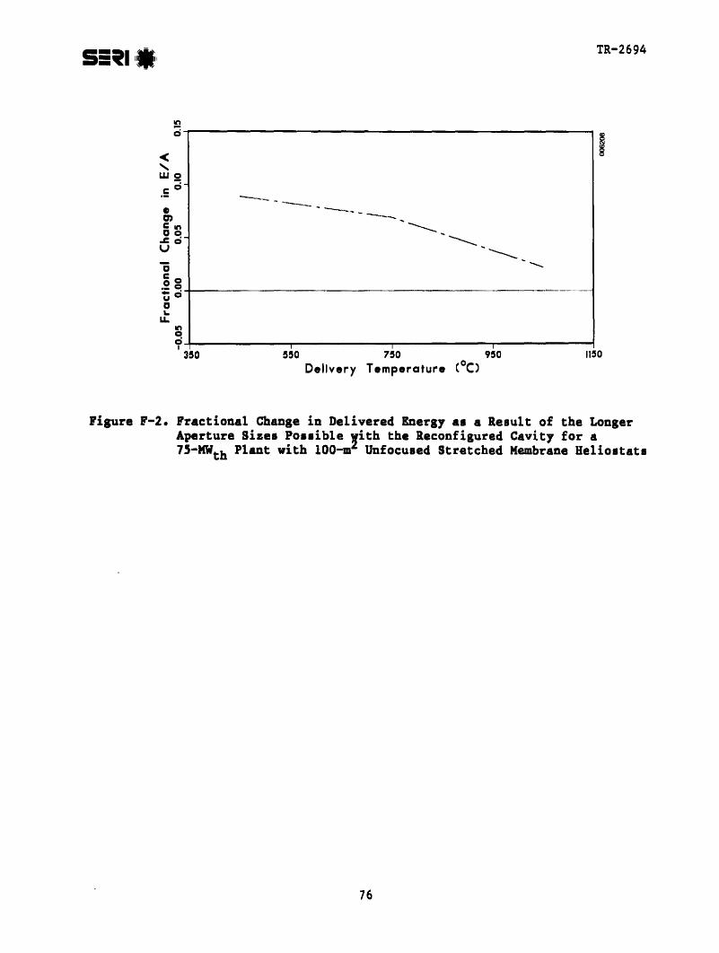
TR-2694

---------------

!!l0--------------------------. !<......wi!.S 0

Ino

~-+--------------.,....------~-----~350 nee

figure f-2. Fractional Change in Delivered EnerlY al a Relult of the LonlerAperture Sizes Poslible lith the Reconfigured Cavity for a75-MWt h Plant with lOO-m Unfoculed Stretched Membrane Helio8tatl

76

Acurex Solar Corporation485 Clyde Ave.Mt. View, CA 94042Mr. Don Duffy

Arizona Public Service CompanyP.O. Box 21666Phoenix, AZ 85036Mr. Eric Weber

BDM Corporation1801 Randolph SEAlbuquerque, NM 87106

Battelle Pacific NW LaboratoryP.O. Box 999Richland, WA 99352Dr. Ben JohnsonMr. Tom WilliamsDr. Kevin Drost

Bechtel CorporationP.O. Box 3965San Francisco, CA 94119Mr. Pascal DeLaquil

Black and Veatch ConsultingEngineers

1500 Meadow Lake ParkwayKansas City, MO 64114Dr. Charles Grosskreutz

Brumleve, Dr. TomConsultant1512 N. Gate RoadWalnut Creek, CA 94598

Colorado State UniversityERCFt. Collins, CO 80523Dr. John Peterka

Dan-Ka Products, Inc.1135 S. Jason StreetDenver, CO 80223Mr. Daniel Sallis

TR-2694

DISTRIBUTION LIST

Department of Energy/HQ1000 Independence Ave., SWWashington, DC 20585Dr. H. ColemanMr. S. GronichMr. C. MangoldMr. M. ScheveMr. Frank Wilkins

El Paso ElectricP.O. Box 982El Paso, TX 79960Mr. James E. Brown

Electric Power Research InstituteP.O. Box 10412Palo Alto, CA 94303Mr. Donald Augenstein

Entech, IncorporatedP.O. Box 612246DFW Airport, TX 75261Mr. Walter Hesse

Falconer Glass Industries, Inc.500 South Work StreetFalconer, NY 14733-1787Mr. Jack South

Georgia Institute of TechnologyAtlanta, GA 30332Dr. Tom Brown

LaJet Energy CompanyP.O. Box 3599Abilene, TX 79604Mr. Monte McGlaun

Martin MariettaP.O. Box 179Denver, CO 80201Mr. Tom Tracey

McDonnell Douglas AstronauticsCompany5301 Bolsa Ave.Huntington Beach, CA 92647Mr. Jim Rogan

77

Meridian Corporation5113 Leesburg PikeSuite 700Falls Church, VA 22041Mr. Oinesh Kumar

Midwest Research Institute425 Volker Blvd.Kansas City, MO 64110Mr. R. L. MartinMr. Jim Williamson

NASA Lewis Research Center21000 Brookpark RoadCleveland, OH 44135Dr. Dennis Flood

NASA-Johnson Space CenterNASA Road One - EPSHouston, TX 77058Mr. William Simon

New Mexico State UniversityMechanical Engineering Dept.P.O. Box 3548Las Cruces, NM 88003Dr. George Mulhollard

Pacific Gas and Electric CompanyMr. Gerry BraunMr. Joe Iannucci3400 Crow Canyon Rd.San Ramon, CA 94583

Rockwell InternationalEnergy Systems Group8900 De Soto Ave.Canoga Park, CA 91304Mr. Tom H. Springer

Sandia National LaboratoriesSolar Department 8453Livermore, CA 94550Mr. J. C. SwearengenMr. A SkinroodMr. R. A. Rinne

Sandia National LaboratoriesSolar Energy Department 6220P.O. Box 5800Albuquerque, NM 87185Mr. John OttsMr. James LeonardMr. Donald Schuler

78

TR-2694

Science Applications, Inc.10401 Rosselle StreetSan Diego, CA 92121Dr. Barry Butler

Solar Energy Industries Association1717 Massachusetts Ave. NW No. 503Washington, DC 20036Mr. Carlo LaPortaMr. David GorenMr. Hal Seilstad

Solar Energy Research Institute1617 Cole Blvd.Golden, CO 80401Mr. B. P. GuptaDr. L. J. ShannonMr. Floyd BlakeMr. John P. ThorntonDr. Meir CarassoDr. David JohnsonDr. Paul SchisselDr. Gordon Gross

Solar Kinetics, Inc.P.O. Box 47045Dallas, TX 75247Mr. Gus Hutchison

Southern California Edison2244 Walnut Grove Ave.Rosemead, CA 91770Mr. Joe Reeves

University of ArizonaCollege of EngineeringTucson, AZ 95721Dr. Kumar Ramohalli

University of ChicagoEnrico Ferni Institute5640 S. Ellis Ave.Chicago, IL 60637Dr. R. WinstonDr. J. Gallagher

University of Houston4800 Calhoun106 SPA BuildingHouston, TX 77004Dr. Alvin HildebrandtDr. Lorin Vant-Hull

207-1W-083M Corporation3M Center Building,St. Paul, MN 55101Mr. David HillMr. Burton A. Benson

79

TR-2694

Document Control r', SERI Report No, 12, NTIS Accession No.

Page SERI/TR-253-26944. Title and SUbtitle

System Performance and Cost Sensitivity Comparisonsof Stretched Membrane Heliostat Reflectors withCurrent Generation Glass/Metal Concepts

7. Author(s) L. M. Murphy, J. V. Anderson, \11. Short,T. Wendelin

9. Performing Organization Name and Address

Solar Energy Research InstituteA Division of Midwest Research Institute1617 Cole BoulevardGolden, Colorado 80401-3393

12. Sponsoring Organization Name and Address

15. Supplementary Notes

3. Recipient's Accession No.

5. Publication Date

December 19856,

8. Performing Organization Rept. No,

10. Project/Task/Work Unit No,

5111.3111, Contract (C) or Grant (G) No.

(C)

(G)

13. Type of Report & Period Covered

Technical Report14.

16. Abstract (Limit: 200 words) He l t ostat costs have long been recogni zed as a major factor 1 nthe cost of solar central receiver plants. Research .on stretched membrane heliostatshas been emphasized because of their potential as a cost-effective alternative tocurrent glass/metal designs. However, the cost and performance potential of stretchedmembrane heliostats from a system perspective has not been studied until this time.The optical performance of individual heliostats is predicted here using results es­tablished in previous structural studies. These performance predictions are used tocompare ·both focused and unfocused stretched membrane heliostats .with state-of-the­art glass/metal heliostats from a systems perspective. We investigated the sensitiv­ity of the relative cost and performance of fields of heliostats to a large numberof parameter variations, including system size, delivery temperature, heliostat mod­ule size, surface specularity, hemispherical reflectance, and macroscopic surfacequality. The results indicate that focused stretched membrane systems should havecomparable performance levels to those of current glass/metal heliostat systems. Further, because of their relatively lower co~t, stretched. membrane heliostats shouldprovide an economically attractive alternative to current glass/metal heliostats overessentially the entire range of design parameters studied. Unfocused stretched mem­brane heliostats may also be attractive fo~ a somewhat more limited range of applica+inn~ ;nr111r1;",I't +h'a ,~·,.."oV' n'~n+ ~;'7t:1~ a nn lnwpr 'delivery temoeratures.17. Document Analysis ....

a. Descriptors Cost ; Heliostats ; Mirrors ; "Optical Systems ; Performance

b. Identifiers/Open-Ended Terms Stretched membrane heliostats

c. UC Categories

62

18, Availability Statement

National Technical Information ServiceU.S. Department of Commerce5285 Port Royal RoadSpringfield, Virginia 22161

Form No.0089 (3-25-82)

19. No. of Pages

96

20, Price

ADS