system stability improvement through optimal control ... gtd... · system stability improvement...

System Stability Improvement through Optimal Control

Allocation in VSC HVDC Links

Journal: IET Generation, Transmission & Distribution

Manuscript ID: GTD-2011-0828.R1

Manuscript Type: Research Paper

Date Submitted by the Author: n/a

Complete List of Authors: Pipelzadeh, Yousef; Imperial College London, Electrical and Electronic Engineering Chaudhuri, Nilanjan Ray; Imperial College London, Electrical and Electronic Engineering; Chaudhuri, Balarko; Imperial College London, Electrical and Electronic Engineering

Green, T.; Imperial College London, Department of Electrical Engineering

Keyword: POWER SYSTEMS, DAMPING, STABILITY, POWER CONTROL, POWER ELECTRONICS

IET Review Copy Only

IET Generation, Transmission & Distribution

System Stability Improvement through Optimal Control

Allocation in VSC HVDC Links

Yousef Pipelzadeh, Nilanjan Ray Chaudhuri, Balarko Chaudhuri, Tim C Green ∗

∗Y Pipelzadeh, N R Chaudhuri, B Chaudhuri and T C Green are with Imperial College London, Lon-don, UK (e-mail: [email protected], [email protected], [email protected],

[email protected])

Page 1 of 31



Abstract

Control of both active and reactive power in voltage source converter (VSC) based High

Voltage Direct Current (HVDC) links could be very effective for system stability improve-

ment. The challenge, however, is to properly allocate the overall control duty among the

available control variables in order to minimize the total control effort and hence allow use

of less expensive converters (actuators). Here relative gain array (RGA) and residue anal-

ysis are used to identify the most appropriate control loops avoiding possible interactions.

Optimal allocation of the secondary control duty between the two ends of the VSC HVDC

link is demonstrated. Active and reactive power modulation at the rectifier end, in a certain

proportion, turns out to be the most effective. Two scenarios, with normal and heavy load-

ing conditions, are considered to justify the generality of the conclusions. Subspace-based

multi-input-multi-output (MIMO) system identification is used to estimate and validate

linearized state-space models through pseudo random binary sequence (PRBS) probing.

Linear analysis is substantiated with non-linear simulations in DIgSILENT PowerFactory

with detailed representation of HVDC links.

1 Introduction

Modulation of the active power order of an High Voltage Direct Current (HVDC) link [1, 2]

could be extremely effective for damping low frequency power oscillations, thereby increasing

the transfer capacity of an AC transmission system. Network operators like WECC have

considered this in 1970s to improve their system dynamic performance [3]. Over the past few

decades a lot of research attention was focused on identifying ways to maximize the impact

of HVDC modulation control on AC system stability [4, 5, 6, 7]. In the recent past, with

an increasing number of HVDC installations around the world, especially in countries with

long transmission corridors like Brazil, China and India, there has been a renewed interest

in this area [8, 9, 10, 11]. Even in smaller countries, such as the U.K. the HVDC links would

increase the stability limits in addition to direct expansion of transmission capacity.

Most of the work on HVDC control to damp oscillations, including those mentioned

2

Page 2 of 31



above, have primarily focused HVDC systems based on Line Commutated Converter (LCC)

based HVDC technology. This, of course, is a proven and mature technology and constitutes

the bulk of the HVDC installations around the world especially, at higher power levels.

Since the first commercial installation of the Voltage Source Converter (VSC) based HVDC

system in the late nineties, its size and use has grown due to its advantages over its LCC

counterpart [1, 2, 12, 13]. Some of the larger VSC installations that are either already

commissioned or about to be in near future include the 400 MW Transbay project in the

US [14], 400 MW BorWin 1 offshore link north of Germany and 600 MW Caprivi link (with

both poles operational) in Namibia [15].

A VSC HVDC link allows independent modulation of both the active and reactive power

(or voltage) at both ends and hence offers more flexibility than LCC systems whereby only

the active power can be modulated. There is tremendous potential for VSC HVDC systems

to contribute towards improvement in AC system dynamic performance as discussed in

[16, 17, 18]. For power oscillation damping through supplementary modulation of active

and/or reactive power in a VSC-HVDC link, the converters dynamic ratings (MVA) are set

not only according to their steady-state values, but also their expected range of modulation

(‘headroom’) during dynamic conditions. There exist multiple control options within a VSC

HVDC in damping inter-area oscillations, which is not well reported in the literature. The

primary objective of this paper is to highlight the importance of allocating the secondary

control duty appropriately among the available options in terms of reducing the overall

control effort (energy). The motivation behind control energy minimization is to invoke

lesser excursion on the control variables around their steady-state values by ensuring that the

control effort demanded from the actuators is optimal. This translates into lower converter

dynamic rating/headroom required and hence, lower associated converter costs since it

would be very expensive to increase a converter station rating to incorporate secondary

controls.

The main research question addressed is: How to optimally allocate the control duty

among the multiple control options that exist within a VSC HVDC for supplementary

damping control, in terms of reducing the overall control energy, and hence, minimizing the

dynamic ratings of the expensive converters?

3

Page 3 of 31



The paper begins by presenting a case study (see Section 2) with a VSC HVDC link

added in parallel with the existing AC tie-lines of a multi-machine test system [19] modelled

in DIgSILENT PowerFactory [20]. In Section 3, linearized state-space model of the system

was estimated by measuring system responses to injecting pseudo random binary sequence

(PRBS) probing signal at the VSC HVDC control inputs, since DIgSILENT does not provide

a linear model directly. This has been a common practice for model validation in field

at WECC and other systems [21]. Numerical algorithm for subspace state-space system

identification (N4SID) [22] which is a proven technique for obtaining linearized state-space

models using input/output data was used. N4SID is particularly useful tool for high-order

multi-variable systems [23]. This technique has been shown to provide accurate linear

models for the SE Australian test system [24]. VSC HVDC offers multiple control-loop

options through modulation of active power (at the rectifier end) and reactive power (at

both ends). In Section 4, residue analysis and relative gain array (RGA) and were used to

identify the most appropriate control-loops avoiding possible interactions [25].

In Section 5, optimal allocation of the secondary control duty between the two ends of

the VSC HVDC link was formulated as a constrained optimization problem. Since it is not

straightforward to solve such a problem analytically [26], a simulation-based design of ex-

periment (DoE) [27] approach which is widely used in industries was adopted to identify an

optimal combination of control options in VSC HVDC. The overall control energy require-

ment was expressed as a function of allocation factors in order to determine the appropriate

combination. Dynamic simulations are presented in Section 6 for two scenarios considering

normal and heavy loading conditions to justify the generality of the conclusions.

2 Test Cases in DIgSILENT PowerFactory

The AC part of the test system considered here is the well known 4-machine, 2-area test

system in [19]. There are four generators (G1, G2 and G3, G4), two in each area (marked

West and East) as shown in Fig. 3. The generators were represented by sub-transient models

and equipped with IEEE DC1A excitation systems [28]. The active component of the loads

at buses 7 and 9 have constant current characteristics, while the reactive components have

4

Page 4 of 31



constant impedance characteristics. The power-flow and dynamic data for the system are

given in [19].

A point-to-point VSC-based HVDC link was added in parallel to the AC corridor be-

tween buses 7 and 9. A single-line diagram for both the LCC system (see Fig. 1) and VSC

HVDC (see Fig. 2) systems with their associated parameters are provided in the Appendix.

The converter and the line ratings of the both DC links were chosen in line with those of

the LCC system in [19]. The AC-DC system was modelled in DIgSILENT PowerFactory

after verifying the AC part against the results in [19].

Out of several operating scenarios considered, two different loading conditions are pre-

sented here. Under normal loading, the power transfer through the 230 kV AC corridor

from West to East is approximately 400 MW. The loads at buses 7 and 9 were adjusted

to simulate a heavy loading scenario with 600 MW tie-line flow. Under both scenarios, the

steady-state active power order for the rectifier was fixed at 200 MW. The reactive power

order was set to maintain close to unity power factor at the terminal AC buses, 7 and 9.

Standard current control strategy in the d− q reference frame was used for the primary

control loops because of the obvious advantages over voltage control strategy [29]. The

limits on direct and quadrature axes current for both the converters were set at 7.5 and

3.75 kA, respectively with standard current limiting logic (from DIgSILENT) in place.

Secondary modulation (control) of Pr , Qr, Vdci and Qi were studied in terms of their

effectiveness to damp inter-area oscillations. All nodes were considered as potential sites

for Phasor Measurement Unit (PMU) feedback, providing time-synchronized phase angle

measurements. The most effective signals were identified and made available at the control

centers at either end of the VSC HVDC link. Appropriate feedback signals for modulating

each of the secondary control variables were chosen systematically as described later in the

paper.

3 Linear Model Estimation and Validation

It is not possible to obtain the linearized system models directly from DIgSILENT. There-

fore, a system identification technique was used to estimate the linear model from the

5

Page 5 of 31



simulated outputs in response to appropriate probing signals at the inputs. Here, the linear

model has 4 control inputs; Pr, Qr, Vdci and Qi, for the VSC HVDC and 11 possible phase

angle measurements available from the PMUs. Identification of such MIMO systems is quite

challenging and gets further complicated with increase in number of output signals [30].

3.1 Probing Signal

Selection of an appropriate probing signal plays an important role in system identification.

Different probing signals, such as repeated pulses, band-limited gaussian white noise, PRBS,

Fourier sequence, have been reported in the literature [30], [31]. Here PRBS was chosen

due to its richer spectrum [30].

At every time step, one of the two pre-specified binary values was generated randomly

by rounding the magnitudes of a complex combination of transcendental functions. The

amplitude of the PRBS was chosen to be high enough to sufficiently excite the critical modes

without pushing the responses into nonlinear behaviour. Persistent excitation of at least the

model order of interest was provided. Moreover, the probing sequence for different inputs

were ensured to be uncorrelated [31]. Typical PRBS injection signals used for probing the

test system are shown in Fig. 4.

3.2 MIMO Subspace Identification

The discrete state space model of the MIMO system with m inputs and l outputs can be

expressed as:

x(k + 1) = Adx(k) + Bdu(k) + w(k)

y(k) = Cdx(k) + Ddu(k) + v(k)(1)

where, Ad ∈ ℜn×n, Bd ∈ ℜn×m, Cd ∈ ℜl×n are the matrices to be estimated and w(k) ∈ ℜn×1

and v(k) ∈ ℜl×1 are non-measurable observation and process noise vector sequences. Here,

the input vector u(k) ∈ ℜ4×1 is the set of PRBS injection signals at the 4 control inputs

of VSC HVDC and the simulated output responses y(k) ∈ ℜ11×1 are the phase angles of

voltage measured from the 11 PMUs.

Using the input probing signal ui(0), ui(1), ...ui(N ), i = 1, 2, ...4 and output responses

yi(0), yi(1), ...yi(N ), i = 1, 2, ...11 the matrices Ad, Bd, Cd and Dd were calculated such

6

Page 6 of 31



that the simulated (actual) data resembled the responses from the estimated (identified)

linear model. The estimated model in discrete domain was converted to continuous domain

for linear analysis and control design. N4SID [22] was used to estimate the above matrices.

A model order of 45 was found to be appropriate for both load scenario.

3.3 Model Validation

To validate the estimated linear model of the MIMO system, pulses of 0.5 s duration were

applied at the 4 control inputs separately and in all possible combinations. The blue (black

in grey-scale) traces in Fig. 5 show the simulated responses from DIgSILENT against the

red (grey in grey-scale) ones which were obtained from the identified linear model. Very

close correlation between the red and blue traces in all cases (only a few representative cases

are shown here) confirms the accuracy of the estimated linear models. These models were

used for eigen value analysis, control loop selection and control allocation described later.

4 Control Loop Selection

4.1 Residue Analysis

Residues provide a combined measure of controllability and observability of the modes of

interest of a linearized system model which can be expressed in state-space form as:

∆x

∆y

=

A B

C D

∆x

∆u

; G(s) ,

A B

C D

(2)

Applying an appropriate transformation, (2) can be transformed into a modal (normal

or decoupled) form [32] as:

z

∆y

=

Λ Φ−1B

CΦ D

z

∆u

(3)

where Λ = Φ−1AΦ is a diagonal matrix and Φ =

[

φ1 φ2 ... φn

]

is the right eigen

vector (or modal) matrix comprising the right eigen vectors (φ1, φ2, ..) corresponding to

7

Page 7 of 31



each mode.

Modal observability Obij of the ith mode in the jth output is obtained by multiplying

the jth row vector of C with the ith column of Φ. Similarly, modal controllability Coik of

the ith mode in the kth control input is the product of the jth row vector of Φ−1 and the

kth column of B.

Coik =[

Φ−1]

i× [B]k (4)

Obij = [C]j × [Φ]i (5)

The product of modal controllability and observability gives the residue Resi−kj =

Coik × Obij which indicates the extent to which mode i can be observed and controlled

through input k and output j. The elements of an eigen vector are complex numbers,

in general, and as such modal controllability Coij, modal observability Obik and residue

Resi−kj are all complex numbers with a magnitude and a phase angle component.

Once the residues corresponding to all possible input-output combinations are calculated

and sorted in descending order of magnitude, the appropriate ones are chosen from the top

(with highest residues) to ensure minimum control effort. For single-input-single-output

(SISO) systems the phase angle of the residue is not important. However, for single-input-

multiple-output (SIMO) or MIMO systems, the phase angle could be critical when choosing

appropriate inputs and outputs [33]. RGA can be an addition to the residue analysis for

a systematic application in large power system studies. It measures two-way interactions

between a determined input and output [34].

4.2 Relative Gain Array (RGA)

RGA provides a measure of interaction between several loops in the case of decentralized

control [35]. For a non-singular square system G(s), the RGA at a particular frequency ω

is a square matrix defined as:

RGA(G(ω)) , Υ(G(ω)) = G(ω)× (G(ω)−1)T (6)

8

Page 8 of 31



where × denotes element-by-element multiplication (the Hadamard or Schur product)

[23]. For non-square systems, the concept can be generalized using the pseudo-inverse.

Suppose that the jth input uj of a MIMO system G(s) is used to control the ith output

yi. This leads to two extreme cases: i) all the other control loops are open, i.e., uk =

0, ∀k 6= j and ii) all other control loops are closed, i.e., with perfect control under steady

state (reasonable approximation for frequencies within the bandwidth) yk = 0, ∀k 6= i. It

can be shown that [23]:

gij ,

(

∂yi

∂uj

)

uk=0,k 6=j

= [G(ω)]ij (7)

gij ,

(

∂yi

∂uj

)

yk=0,k 6=i

= [G(ω)−1]ji (8)

The ijth element of the RGA [Υ(G)]ij captures the ratio υij between the gains gij and

gij, corresponding to the two extremes, and thus provide a useful measure of interaction.

υij ,gij

gij

= [G(ω)]ij[G(ω)−1]ji = [Υ(G(ω))]ij (9)

For an m×m MIMO system with m inputs and m outputs there are m! ways in which

the control loops can be arranged. Looking at the RGA and following the rules stated below,

appropriate control loops can be selected in a systematic way avoiding the ones which are

likely to cause adverse interaction.

1. Choose to pair those inputs and outputs for which the RGA element in the crossover

frequency range is close to 1.

2. In order to minimize adverse interactions, avoid input-output pairing where the RGA

elements calculated at low frequency (steady-state) are negative.

In this paper, the second criterion is used to select appropriate input-output pairs for

the two terminals of a VSC HVDC system.

9

Page 9 of 31



5 Control Allocation

For a MIMO system G(s) with m-inputs and m-outputs, the overall control duty can be

allocated (distributed) amongst individual input-output pairs resulting in a diagonal m-

input, m-output controller K(s). The control allocation is said to be ‘optimal’ when the

overall control effort (control energy) is minimum. Such an optimal control allocation

problem can be expressed mathematically as follows:

G(s) ,

A B

C 0

; A ∈ ℜn×n, B ∈ ℜn×m, C ∈ ℜm×n (10)

The objective is to determine the control allocation factors αi and a stable diagonal con-

troller K(s),

K(s) ,

Ak Bk

Ck Dk

=

Ak1 0 . 0 Bk1 0 . 0

0 Ak2 . 0 0 Bk2 . 0

. . . . . . . .

0 0 . Akm 0 0 . Bkm

Ck1 0 . 0 0 0 . 0

0 Ck2 . 0 0 0 . 0

. . . . . . . .

0 0 . Ckm 0 0 . 0

(11)

Akj ∈ ℜnk×nk, Bkj ∈ ℜnk×1, Ckj ∈ ℜ1×nk, j = 1, 2, · · · , m

which minimizes the cost function J:

minJK(s),αi

=

∞∫

0

m∑

i=1

∆u2i dt (12)

10

Page 10 of 31



such that the following constraints are satisfied:

m∑

i=1

αi = 1 (13)

K(s) ∈ S (14)

∆λc

A BiCki

BkiCi Ak

∈ (λd − λo)αi ∀ i = 1, · · · , m (15)

λc

A BCk

BkC Ak

∈ λd (16)

nk ≪ n (17)

where, ∆ui: dynamic variation of ith control input, λc(·): critical eigen values, ∆λc(·): shift

of critical eigen values towards left of the complex plane, λo = λc[G(s)]: critical eigen values

of the open loop system G(s), S: set of stable controllers and λd: desired region for the

critical eigen values. Bi : ith column of the plant input matrix B, Ci : ith row of the plant

output matrix C, Bki : ith column of the controller input matrix Bk, Cki : ith row of the

controller output matrix Ck.

The objective in (12) represents minimization of overall control energy. Constraint (13)

indicates that the sum of all the control allocation factors αi should be 1. Each control input

i would contribute to the overall shift of the critical eigen values (λd − λo) in proportion

to the control duty αi allocated to it, which is captured in constraint (15). Constraint

(16) represents the placement of the critical closed-loop eigen values (with all control loops

closed) at desired location (λd) with a diagonal (decentralized) controller.

It is not straightforward to analytically solve the constrained optimization problem de-

scribed above to determine αi and K(s). Here the solution was sought through a simulation

based design of experiments (DoE) approach [27]. A number of scenarios with random com-

binations of control allocation factors αi ∈ 0 : 1, Σαi = 1 were generated. A decentralized

controller K(s) was designed for each combination to satisfy (14). The cost function J was

evaluated from simulation results for each case. Using the data from several trials, J was

expressed as a function of αi from which the optimum control allocation factors and the

11

Page 11 of 31



corresponding controller K(s) could be synthesized. Moreover, pareto of each control input

i on the overall control energy (indicated by cost function J) could also be evaluated.

6 Results and Discussions

6.1 Eigen value Analysis

The linear model of the system was identified using a subspace identification technique

(N4SID) described in Section 3.2. Table 1 shows the damping ratios and frequencies of the

critical modes of the system under normal loading (400 MW tie-flow) and heavy loading

(600 MW tie-flow) conditions.

Table 1: Damping ratios and frequencies of critical modes. VSC HVDC operates in P − Q

control on the rectifier end, and Vdc −Q control on the inverter end. LCC HVDC operates

in P control on the rectifier end, and Vdc control on the inverter end. See Appendix.Loading AC system only with VSC HVDC with LCC HVDC

Condition ζ, % f, Hz ζ, % f, Hz ζ, % f, Hz

Normal 0.6 0.519 1.5 0.568 1.4 0.578

8.5 1.058 8.4 1.062 9.3 1.055

8.3 1.089 7.9 1.097 9.2 1.086

Heavy -7.8 0.401 0.7 0.54 0.9 0.548

8.4 1.076 8.6 1.06 8.0 1.0718.9 1.05 7.7 1.092 5.4 1.112

Under the normal condition and with the DC link removed, one poorly-damped inter-

area mode at 0.52 Hz and two local modes at 1.06 and 1.09 Hz are present. With the

introduction of the VSC HVDC link, the frequency of the inter-area mode increases to

0.568 Hz while the damping ratio improves from 0.6% to 1.5%. As the DC link takes a

200 MW share of the total tie-flow, the power angle across the corridor decreases, thereby

increasing the synchronizing torque coefficient and in turn, the frequency [19].

Under the heavy loading condition, the AC system alone is unstable but the inclusion of

VSC HVDC stabilizes the system (damping ratio increases from -7.8% to 0.7%) by taking

200 MW of the tie-flow and giving reactive power support at each end. As expected, an

increase in the frequency of the inter-area mode from 0.4 Hz to 0.54 Hz is also observed.

A comparison with the inclusion of a LCC HVDC link with same rating as in [19] shows

that the frequency under normal and heavy loading scenarios increases to 0.578 Hz and

12

Page 12 of 31



0.548 Hz, respectively, see Table 1. In all cases the system is better damped with HVDC.

6.2 Control Loop Selection

In this work a decentralized control framework is used at the rectifier and inverter end

control centers, see Fig. 3. There are 4 possible control (modulation) inputs Prmod, Qrmod,

Vdcimod and Qimod, and 11 possible outputs ( the phase angles measured by the PMUs

installed at 11 buses). Residues were calculated for all possible input-output combinations.

The magnitudes and phase angles of the residues under normal loading condition are shown

in Table 2.

Table 2: Residues with measured phase angles of voltages at 11 buses and 4 control inputs

of the VSC HVDC under normal loading conditionbus Prmod Qrmod Vdcimod Qimod

no. mag ang mag ang mag ang mag ang

1 1.0 -87 0.64 88 0.06 12 0.67 -99

2 0.91 -88 0.59 88 0.06 12 0.61 -99

4 0.17 -106 0.11 70 0.01 -5 0.11 -117

5 0.95 -88 0.61 88 0.06 12 0.64 -99

6 0.86 -88 0.55 88 0.05 12 0.57 -100

7 0.77 -88 0.50 87 0.05 11 0.52 -100

8 0.47 -91 0.30 84 0.03 8 0.32 -103

9 0.21 -102 0.13 74 0.01 -1 0.14 -114

10 0.18 -104 0.12 72 0.01 -3 0.13 -115

11 0.15 -108 0.10 67 0.01 -8 0.10 -120

Since Vdcimod has very small residue, only Prmod, Qrmod, and Qimod were considered for

secondary control. Three measured outputs - phase angles at buses 1, 2 and 5 (marked in

bold) - were chosen for reliability in order of descending residue magnitudes.

RGA at steady-state (see Section 4.2) was used to form appropriate input-output pair

among Prmod, Qrmod, and Qimod and phase angles at buses 1,2 and 5. Any input-output

pair with negative RGA element were discarded to avoid adverse interactions. Based on

the RGA elements in Table 3 for normal loading condition, bus angle 5 was chosen for

Prmod, bus angle 2 for Qimod and 1 for Qrmod to form a 3-input, 3-output decentralized

control structure. Similarly, for heavy loading condition, bus angles 5, 1 and 2 were paired

to Qrmod, Prmod and Qimod, respectively. The RGA elements corresponding to the chosen

input-output pairs are marked in bold in Table 3.

13

Page 13 of 31



Table 3: RGA for possible input-output combinationsbus Normal Loading Heavy Loading

no. Prmod Qrmod Qimod Prmod Qrmod Qimod

1 -10.93 12.48 -0.54 216.86 -222.33 6.46

2 -24.84 11.76 4.08 399.34 -431.38 33.04

5 36.78 -23.24 -12.53 -615.20 654.71 -38.50

6.3 Control Allocation

As previously discussed in Section 5, the objective here is to optimally allocate/distribute

the overall control duty between the rectifier and inverter end variables such that the overall

control energy required is minimum. Only Prmod, Qrmod and Qimod are considered leaving

out Vdcimod due to low residues, see Table 2.

Parameters α1, α2 represents the fraction of the control duty allocated to Prmod and

Qrmod, respectively while α3 = 1− (α1 + α2) is the share of Qimod. A design of experiment

(DoE) with several random (but permissible) combinations of αi ∈ 0, 1; Σαi = 1 was

conducted. A diagonal 3-input, 3-output controller was designed in each case with the

appropriate control loops described in Section 6.2. The specification for control design was

to ensure a minimum settling time Ts = 10.0 s for the critical inter-area mode. Non-linear

simulations in DIgSILENT PowerFactory were carried out to calculate the overall control

energy J from time variations of Prmod, Qrmod and Qimod, see Fig. 13, in each case:

J =

∞∫

0

[

Prmod(t)2 + Qrmod(t)

2 + Qimod(t)2]

dt (18)

A three phase self-clearing fault near bus 9 (the inverter bus) was considered for the heavy

loading condition, whereas under the normal loading scenario fault near bus 8 was simulated.

Using the simulation based DoE results, a function relating J to the two independent

variables α1, α2 was constructed as:

J = (α1, α2) ∀α1, α2 ∈ 0, 1; (α1 + α2) ≤ 1 (19)

A representative result is shown in Fig 6 for the heavy loading condition (see Section 6).

More control energy is required towards either extreme 0 : 1 of α2 axis indicating the fact

14

Page 14 of 31



that an appropriate combination of control variables at both ends could be more effective

than exercising only the rectifier or inverter end options. For both normal and heavy loading

similar trends were observed. However, the control energy required for the heavy loading is

much more than for the normal loading condition because of the larger power transfer and

the fault near the inverter bus (bus 9).

The bar graphs in Figs 7 and 8 show the minimum control energies for the following

options:

Pr: P control at rectifier end only, α1 = 1, α2 = 0;

Qr: Q control and rectifier only, α1 = 0, α2 = 1;

Qi: Q control at inverter only, α1 = 0, α2 = 0;

Pr−Qr : P and Q control at rectifier only, α1 = α1opt, α2 = α2opt ∀α1, α2 ∈ 0, 1; (α1+α2) =

1;

Pr − Qi: P at rectifier and Q control at inverter, α1 = α1opt, α2 = 0;

Qr − Qi: Q control at both rectifier and inverter, α1 = 0, α2 = α2opt;

Pr − Qr − Qi: P, Q at rectifier and Q control at inverter, α1 = α1opt, α2 = α2opt.

7 Simulation Results

This Section shows a representative set of time-domain simulation results in DIgSILENT

PowerFactory for the cases considered in Figs 7 and 8.

7.1 Normal Loading Condition

The dynamic performance of the system for different secondary control loop combinations

is shown in Figs 9 and 10.

A three-phase fault at bus 8 that self-clears after 5 cycles is considered. Note that the

legends marked on the top right corner of the figures indicate the control loop combinations

while the plotted variables are described below each subplot.

In all cases the desired settling time of around 10.0 s is achieved. With Pr control, see

subplots 9(a), 9(b), 9(c), 9(d), Idr varies while Iqr is nearly zero to maintain unity power

factor. For Qr and Qi control Iqr and Iqi are seen to vary in subplots 9(f), 9(h). The high

15

Page 15 of 31



frequency components are due to successive hitting of the current limits immediately after

the large disturbance. Fig. 10 shows the dynamic performance with more than one control

loop. For Pr − Qr pairing, see subplots 10(a), 10(b), both Idr and Iqr changes. In all the

cases Vdci is kept constant - a representative plot is shown for the case with Pr −Qi pairing,

see subplot 10(d).

7.2 Heavy Loading Condition

Figs 11 and 12 show the dynamic behavior of the system following a three-phase self-clearing

fault for 5 cycles near the inverter bus (bus 9).As expected a settling time of about 10.0 s

is achieved under this heavy loading condition with a 600 MW tie flow, see subplot 11(a).

During the fault, the dc bus voltages at both the ends increase sharply due to reduction of ac

side power transfer. This is followed by oscillations in Vdcr due to the dc link dynamics while

the Vdci is regulated to a constant value, see subplots 11(c), 11(d). Dynamic performance of

the system with a combination of control loops is shown in Fig. 12. Because of the severity

of the fault close to inverter bus Idr and Iqr are seen to violate their respective limits, see

subplots 12(a), 12(b).

Fig. 13 shows the outputs of the controllers for different combinations of secondary con-

trol loops. These plots confirm that the control effort needed with modulation of Pr is much

less compared to Qr modulation. Similarly control effort required for Qr − Qi combination

is larger than other alternatives except Qi. Interestingly, Pr−Qr−Qi combination demands

higher control energy as compared to the Pr −Qr and Pr −Qi cases. The range of variation

of the system variables is higher in Figs 11 and 12 compared to Figs 9 and 10 because of

heavy loading condition and fault close to the inverter bus. To summarize, similar dynamic

performance (10.0 s settling time in this case) can be obtained through different combina-

tions of rectifier and inverter end control parameters (Pr, Qr and Qi). However, less control

energy is required when control duty is allocated/distributed in a proper way.

16

Page 16 of 31



8 Conclusions

In this paper, the importance of properly allocating the secondary control duty at both

ends of a VSC HVDC link is highlighted. For the case study presented, active and reactive

power modulation at the rectifier end (in a certain proportion) is shown to be the most

effective in terms of minimum overall control energy (effort) required. This was true for

both normal as well as heavy loading conditions with short-circuit faults at various locations.

However, this need not be a general conclusion for other systems and would depend on the

type and distribution of loads with respect to the HVDC terminals and also the power

flow patterns. Nonetheless, the significance of considering the control allocation aspect in

order to reduce the overall control energy and hence the headroom required from expensive

actuators (terminal converters in this case) is demonstrated.

Although the test system used for this study is relatively small, it is widely reported in

the literature for inter-area oscillations studies. It is used as a first step for developing a

basic understanding of the proposed concept. The simulation-based design of experiment

(DoE) approach is popular in industries and is used here to demonstrate that there exists

an optimal combination of control options in VSC HVDC. This paper thus should set the

motivation for future work on systematic and elegant control design techniques to address

this problem on larger networks with many controllable devices. With increasing penetra-

tion of controllable power electronics in the form of FACTS, HVDC, wind generators etc.

appropriate control allocation is going to be crucial in future.

Acknowledgment

The authors would like to acknowledge the suggestions received from Dr Rajat Majumder

at Siemens Energy, USA and from the DIgSILENT support team.

17

Page 17 of 31



Appendix

LCC HVDC Model

A single-line diagram representing the LCC HVDC, as modelled in PowerFactory DIgSI-

LENT is shown in Fig. 1. The system parameters are provided in Table 4. The converter

and the line ratings of the LCC HVDC link were chosen in line with those of the LCC

system in [19].

Xc

RL LL

dc line

Smoothing

Reactor, L

Xc

Reactive PowerSupport

dc

filter

dcI

Vdc 2

PinvQinv

Qrated Vdc

2

Vt Vdc PVPCC

Figure 1: Single-line diagram of the bipolar LCC HVDC system

Table 4: LCC HVDC parametersName Parameter Value

Rectifier control mode Rec, control P

Inverter control mode Inv, control Vdc

Converter rating Srating 224 MVA

DC line voltage Vdc 56 kV

DC line current Idc 3.6 kA

DC line resistance RL 0.15 Ω

DC line inductance LL 100 mH

Commutating reactance Xc 0.57 Ω

Smoothing reactor L 50 mH

Rated reactive power Qrated 125 MVAr

Terminal ac voltage Vt 30 kV

Terminal PCC voltage (grid) VPCC 230 kV

Firing angle set-point α 15 deg

Extinction angle (gamma) set-point γ 25 deg

18

Page 18 of 31



VSC HVDC Model

A single-line diagram representing the VSC HVDC system, as modelled in PowerFactory

DIgSILENT is shown in Fig. 2. The system parameters are provided in Table 5. The

converter and the line ratings of the VSC HVDC link were chosen to match those of the

LCC system.

iac, abc

Idc

RL

Vdc -QP-QC

C

C

C

recP

RL LL

Rc Lc Rc Lc

Qrec

Vdc 2

Vdc 2

PinvQinv

LL

VPCC Vt

Figure 2: Single line diagram of the VSC HVDC system

Table 5: VSC HVDC parametersName Parameter Value

Rectifier control mode Rec, control P − Q

Inverter control mode Inv, control Vdc − Q

Converter rating Srating 224 MVA

DC line voltage Vdc 56 kV

DC line current Idc 3.6 kA

Capacitor C 1 mF

DC line resistance RL 0.15 Ω

DC line inductance LL 100 mH

Series reactor inductance Lc 269 mH

Series reactor resistance Rc 0.0 Ω

Terminal ac rated voltage Vt 30 kV

Terminal PCC voltage (grid) VPCC 230 kV

19

Page 19 of 31



References

[1] J. Arrillaga, Y. H. Liu, and N. R. Watson, Flexible power transmission: the HVDC

options. John Wiley, 2007.

[2] V. K. Sood, HVDC and FACTS controllers: applications of static converters in power

systems. Boston; London: Kluwer Academic Publishers, 2004.

[3] R. L. Cresap, W. A. Mittelstadt, D. N. Scott, and C. W. Taylor, “Operating expe-

rience with modulation of the pacific HVDC intertie,” IEEE Transactions on Power

Apparatus and Systems, vol. PAS-97, no. 4, pp. 1053–1059, 1978.

[4] D. E. Martin, W. K. Wong, D. L. Dickmander, R. L. Lee, and D. J. Melvold, “Increas-

ing WSCC power system performance with modulation controls on the intermountain

power project HVDC system,” IEEE Transactions on Power Delivery, vol. 7, no. 3,

pp. 1634–1642, 1992.

[5] T. Smed and G. Andersson, “Utilizing HVDC to damp power oscillations,” IEEE

Transactions on Power Delivery, vol. 8, no. 2, pp. 620–627, 1993.

[6] C. W. Taylor and S. Lefebvre, “HVDC controls for system dynamic performance,”

IEEE Transactions on Power Systems, vol. 6, no. 2, pp. 743–752, 1991.

[7] K. W. V. To, A. K. David, and A. E. Hammad, “A robust co-ordinated control scheme

for HVDC transmission with parallel ac systems,” IEEE Transactions on Power De-

livery, vol. 9, no. 3, pp. 1710–1716, 1994.

[8] M. Xiao-ming and Z. Yao, “Application of HVDC modulation in damping electrome-

chanical oscillations,” in proceedings of IEEE Power Engineering Society General Meet-

ing, 2007, pp. 1–6.

[9] J. He, C. Lu, X. Wu, P. Li, and J. Wu, “Design and experiment of wide area HVDC sup-

plementary damping controller considering time delay in china southern power grid,”

IET Generation, Transmission & Distribution, vol. 3, no. 1, pp. 17–25, 2009.

20

Page 20 of 31



[10] P. Li, X. Wu, C. Lu, J. Shi, J. Hu, J. He, Y. Zhao, and A. Xu, “Implementation of

CSG’s wide-area damping control system: Overview and experience,” in proceedings of

IEEE/PES PSCE Power Systems Conference and Exposition, 2009, pp. 1–9.

[11] L. Li, X. Wu, and P. Li, “Coordinated control of multiple HVDC systems for damping

interarea oscillations in CSG,” in proceedings of IEEE PowerAfrica Power Engineering

Society Conference and Exposition in Africa, 2007, pp. 1–7.

[12] L. Zhang, H. Nee, and L. Harnefors, “Analysis of stability limitations of a vsc-hvdc link

using power-synchronization control,” IEEE Transactions on Power Systems, no. 99,

pp. 1–1, 2011.

[13] L. Zhang, L. Harnefors, and H. Nee, “Interconnection of two very weak ac systems

by vsc-hvdc links using power-synchronization control,” IEEE Transactions on Power

Systems, no. 99, pp. 1–12, 2010.

[14] HVDC PLUS. [Online]. Available: www.siemens.com

[15] HVDC Light. [Online]. Available: www.abb.com

[16] L. Zhang, L. Harnefors, and P. Rey, “Power system reliability and transfer capability

improvement by VSC-HVDC,” in proceedings of Cigre Regional Meeting 20007, 2007.

[17] H. F. Latorre, M. Ghandhari, and L. Soder, “Use of local and remote information in

POD control of a VSC-HVDC,” in proceedings of PowerTech, 2009 IEEE Bucharest,

2009, pp. 1–6.

[18] R. Si-Ye, L. Guo-Jie, and S. Yuan-Zhang, “Damping of power swing by the control of

VSC-HVDC,” in proceedings of IPEC 2007 International Power Engineering Confer-

ence, 2007, pp. 614–618.

[19] P. Kundur, Power system stability and control, ser. The EPRI power system engineering

series. New York; London: McGraw-Hill, 1994.

[20] Digsilent. [Online]. Available: http://www.digsilent.de/

21

Page 21 of 31



[21] J. F. Hauer, W. A. Mittelstadt, K. E. Martin, J. W. Burns, H. Lee, J. W. Pierre, and

D. J. Trudnowski, “Use of the wecc wams in wide-area probing tests for validation of

system performance and modeling,” IEEE Transactions on Power Systems, vol. 24,

no. 1, pp. 250–257, 2009.

[22] P. v. Overschee and B. L. R. d. Moor, Subspace identification for linear systems :

theory, implementation, applications. Boston ; London: Kluwer Academic, 1996.

[23] S. Skogestad and I. Postlethwaite, Multivariable feedback control: analysis and design.

Chichester: Wiley, 1996.

[24] Y. Pipelzadeh, B. Chaudhuri, and T. Green, “Coordinated damping control through

multiple hvdc systems: A decentralized approach,” in 2011 IEEE Power and Energy

Society General Meeting,. IEEE, 2011, pp. 1–8.

[25] L. Zhang, P. X. Zhang, H. F. Wang, Z. Chen, W. Du, Y. J. Cao, and S. J. Chen,

“Interaction assessment of FACTS control by RGA for the effective design of FACTS

damping controllers,” IEE Proceedings Generation, Transmission and Distribution,,

vol. 153, no. 5, pp. 610–616, 2006.

[26] B. Chaudhuri and B. Pal, “Robust damping of multiple swing modes employing global

stabilizing signals with a TCSC,” in IEEE Power Engineering Society General Meeting,

vol. 2, 2004, p. 1709.

[27] D. C. Montgomery, Design and analysis of experiments, 7th ed. Hoboken: John Wiley

& Sons, 2009.

[28] “IEEE std 421.5 - 2005, IEEE recommended practice for excitation system models for

power system stability studies,” pp. 1–85, 2006.

[29] C. Schauder and H. Mehta, “Vector analysis and control of advanced static var com-

pensators,” IEE Proceedings on Generation, Transmission and Distribution, vol. 140,

no. 4, pp. 299–306, 1993.

[30] P. E. Wellstead and M. B. Zarrop, Self-tuning Systems. Control and Signal Processing.

John Wiley & Sons, 1991.

22

Page 22 of 31



[31] T. C. Hsia, System identification: least-squares method. [S.l.]: Lexington Books, 1977.

[32] T. Kailath, Linear systems. Englewood Cliffs; London: Prentice-Hall, 1980.

[33] S. Ray, B. Chaudhuri, and R. Majumder, “Appropriate signal selection for damping

multi-modal oscillations using low order controllers,” in proceedings of IEEE Power

Engineering Society General Meeting, 2008, Pittsburgh, 2008.

[34] J. Milanovic and A. Duque, “Identification of electromechanical modes and placement

of psss using relative gain array,” IEEE Transactions on Power Systems, vol. 19, no. 1,

pp. 410–417, 2004.

[35] E. H. Bristol, “Dynamic effects of interaction,” in proceedings IEEE Conference on

Decision and Control, vol. 16, 1977, pp. 1096–1100.

23

Page 23 of 31



List of captions

Figure 1 Single line diagram of the LCC HVDC system

Figure 2 Single line diagram of the VSC HVDC system

Figure 3 4-machine, 2-area test system with a VSC HVDC link. Secondary control loops

with PMU signals are shown.

Figure 4 Typical PRBS injection used for system identification

Figure 5 Linear model validation with a pulse at different input pairings. Legends in top

right corner of the plots show the secondary control loops used. Legends below the

plots show the variables plotted.

Figure 6 Overall control energy required for different control allocation levels under heavy

loading

Figure 7 Minimum control energy required for each control loop pairing under normal

loading

Figure 8 Minimum control energy required for each control loop pairing under heavy load-

ing

Figure 9 Dynamic performance of the system under normal loading. Legends on top right

corner show the secondary control loops used. Plotted variables described below each

subplot

Figure 10 Dynamic performance of the system under normal loading. Legends on top right

corner show the secondary control loop combinations used.Plotted variables described

below each subplot.

Figure 11 Dynamic performance of the system under heavy loading. Legends on top right


subplot.

24

Page 24 of 31



Figure 12 Dynamic performance of the system under heavy loading. Legends on top right


subplot.

Figure 13 Control effort for different control loop combinations under heavy loading. Leg-

ends on top right corner show the secondary control loops used. Plotted variables

described below each subplot.

25

Page 25 of 31



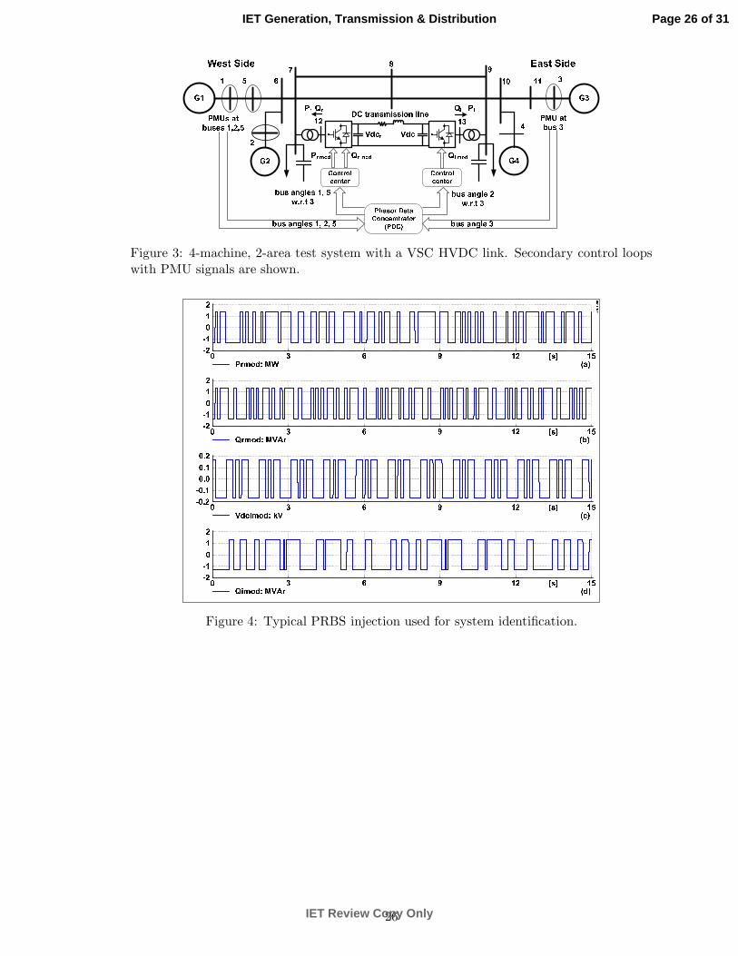
Figure 3: 4-machine, 2-area test system with a VSC HVDC link. Secondary control loopswith PMU signals are shown.

Figure 4: Typical PRBS injection used for system identification.

26

Page 26 of 31



15129630 [s]

1.10.70.2

-0.2-0.7-1.1

Identified model: bus1 - bus3, deg (a)

Actual model: bus1 - bus3, deg (a)

15129630 [s]

0.70.40.1

-0.1-0.4-0.7

Identified model: bus8 - bus3, deg (b)

Actual model: bus8 - bus3, deg

15129630 [s]

0.3

0.2

0.1

-0.1

-0.2

-0.3

Identified model: bus9 - bus3, deg (d)


15129630 [s]

0.6

0.4

0.1

-0.1

-0.4

-0.6

Identified model: bus2 - bus3, deg (c)


15129630 [s]

1.50.90.3

-0.3-0.9-1.5

Identified model: bus6 - bus3, deg (e)


15129630 [s]

2.41.40.5

-0.5-1.4-2.4

Identified model: bus1 - bus3, deg (f)


15129630 [s]

1.50.90.3

-0.3-0.9-1.5

Identified model: bus 2- bus3, deg (h)


15129630 [s]

0.30.20.1

-0.1-0.2-0.3

Identified model: bus7 - bus3, deg (g)


Pr Pr

Pr-Qr-Qi-UiQr-Qi

Pr-Qi Pr-Qi

Qr Qr

400MW 600MW

DIg

SIL

EN

T

Figure 5: Linear model validation with a pulse at different input pairings. Legends in topright corner of the plots show the secondary control loops used. Legends below the plots

show the variables plotted.

0

0.5

1

00.5

1

1.5

2

2.5

3

3.5

4

α2

600 MW tie flow

α1

co

ntr

ol e

ne

rgy,

MV

A2−

s

2

2.5

3

3.5x104

x104

Figure 6: Overall control energy required for different control allocation levels under heavyloading.

27

Page 27 of 31



Pr Qr Qi Pr−Qr Pr−Qi Qr−QiPr−Qr−Qi1000

1500

2000

2500

3000

min

imum

contr

ol energ

y, M

VA2

−s

400 MW tie−flow

7094 6807

Figure 7: Minimum control energy required for each control loop pairing under normal

loading.

Pr Qr Qi Pr−Qr Pr−Qi Qr−QiPr−Qr−Qi15000

20000

25000

min

imum

contr

ol energ

y, M

VA2

−s

600 MW tie−flow

37030 38378

Figure 8: Minimum control energy required for each control loop pairing under heavy

loading.

28

Page 28 of 31



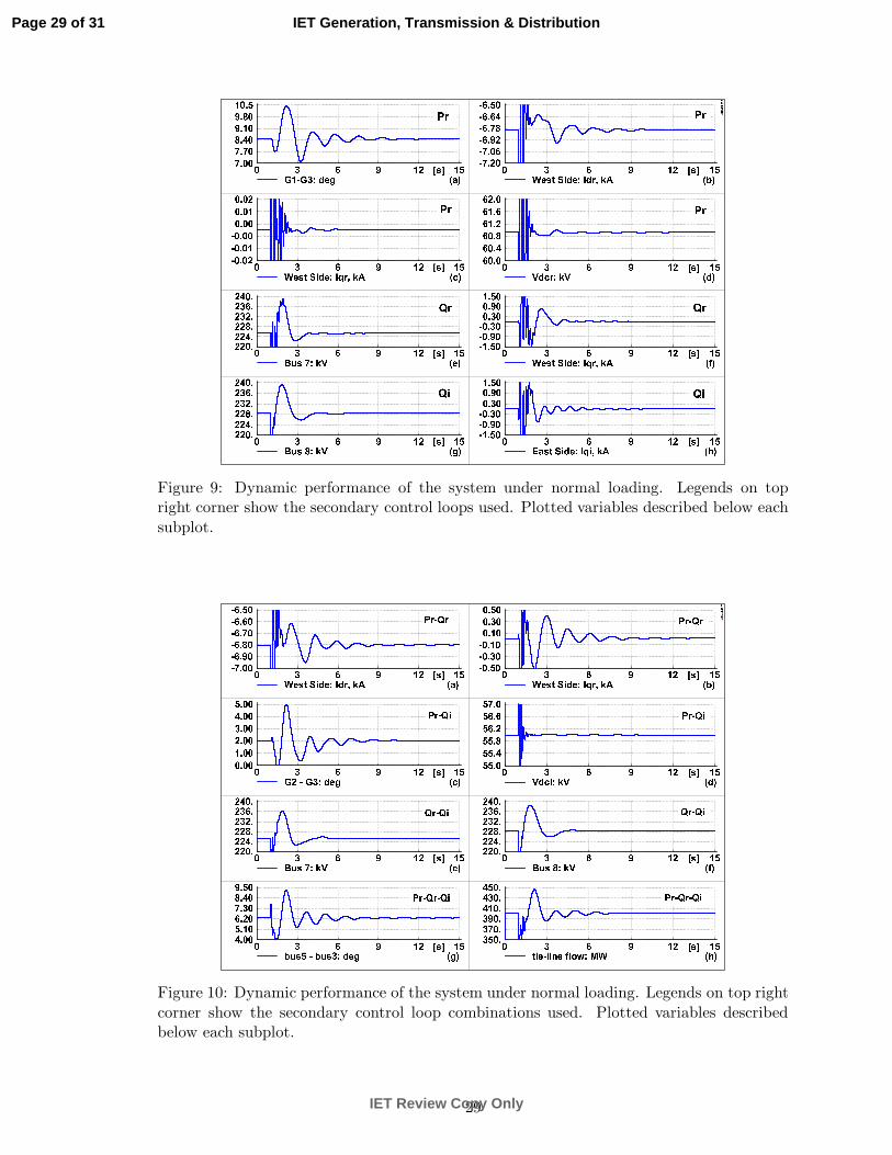
Figure 9: Dynamic performance of the system under normal loading. Legends on topright corner show the secondary control loops used. Plotted variables described below each

subplot.

Figure 10: Dynamic performance of the system under normal loading. Legends on top right

corner show the secondary control loop combinations used. Plotted variables describedbelow each subplot.

29

Page 29 of 31



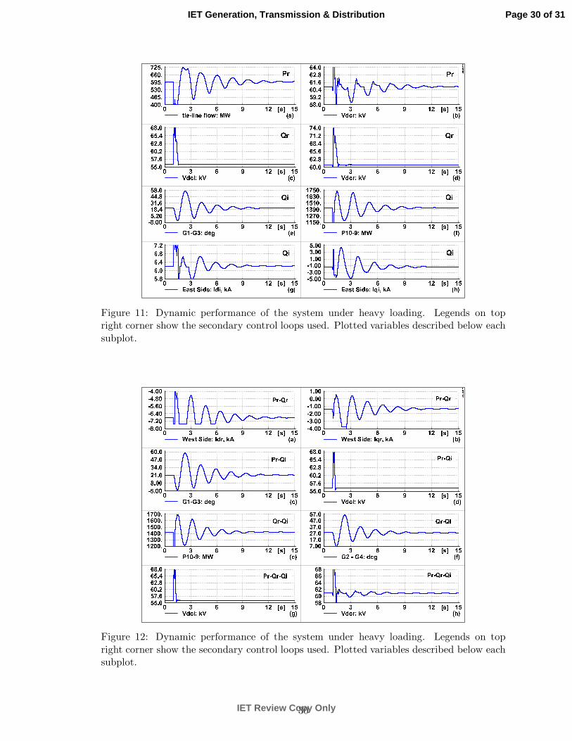
Figure 11: Dynamic performance of the system under heavy loading. Legends on topright corner show the secondary control loops used. Plotted variables described below each

subplot.

Figure 12: Dynamic performance of the system under heavy loading. Legends on top

right corner show the secondary control loops used. Plotted variables described below eachsubplot.

30

Page 30 of 31



Figure 13: Control effort for different control loop combinations under heavy loading. Leg-

ends on top right corner show the secondary control loops used. Plotted variables describedbelow each subplot.

31

Page 31 of 31



system stability improvement through optimal control ... gtd... · system stability improvement...

Documents