systematic assessment of terrestrial biogeochemistry in ...systematic assessment of terrestrial...

Systematic assessment of terrestrial biogeochemistry incoupled climate–carbon models

J A M E S T . R A N D E R S O N *, F O R R E S T M . H O F F M A N w , P E T E R E . T H O R N T O N z, § ,

N A T A L I E M . M A H O WA L D } , K E I T H L I N D S AY z, Y E N - H U E I L E E z,C Y N T H I A D . N E V I S O N *, k, S C O T T C . D O N E Y **, G O R D O N B O N A N z,R E T O S T O C K L I w w , zz, C U R T I S C O V E Y § § , S T E V E N W. R U N N I N G } } and I N E Z Y. F U N G kk*Department of Earth System Science, Croul Hall, University of California, Irvine, CA 92697, USA, wOak Ridge National

Laboratory, Computational Earth Sciences Group, PO Box 2008, Oak Ridge, TN 37831, USA, zClimate and Global Dynamics,

National Center for Atmospheric Research, PO Box 3000, Boulder, CO 80307, USA, §Oak Ridge National Laboratory,

Environmental Sciences Division, PO Box 2008, Oak Ridge, TN 37831, USA, }Department of Earth and Atmospheric Sciences,

2140 Snee Hall, Cornell University, Ithaca, NY 14850, USA, kInstitute for Arctic and Alpine Research (INSTAAR), University of

Colorado, Boulder, CO 80309, USA, **Department of Marine Chemistry and Geochemistry, MS 25, Woods Hole Oceanographic

Institution, Woods Hole, MA 02543, USA, wwDepartment of Atmospheric Sciences, Colorado State University, Ft Collins, CO

80523, USA, zzMeteoSwiss, Climate Service, Federal Office of Meteorology and Climatology, CH-8044 Zurich, Switzerland,

§§Program for Climate Model Diagnosis and Intercomparison, 7000 East Avenue, Bldg. 170, L-103, Livermore, CA 94550-9234,

USA, }}Numerical Terradynamic Simulation Group, College of Forestry & Conservation, University of Montana, Missoula, MT

59812, USA, kkDepartment of Earth and Planetary Science and Department of Environmental Science, Policy, and Management,

307 McCone, Mail Code 4767, University of California, Berkeley, CA 94720, USA

Abstract

With representation of the global carbon cycle becoming increasingly complex in climate

models, it is important to develop ways to quantitatively evaluate model performance

against in situ and remote sensing observations. Here we present a systematic frame-

work, the Carbon-LAnd Model Intercomparison Project (C-LAMP), for assessing terres-

trial biogeochemistry models coupled to climate models using observations that span a

wide range of temporal and spatial scales. As an example of the value of such

comparisons, we used this framework to evaluate two biogeochemistry models that are

integrated within the Community Climate System Model (CCSM) – Carnegie-Ames-

Stanford Approach0 (CASA0) and carbon–nitrogen (CN). Both models underestimated

the magnitude of net carbon uptake during the growing season in temperate and boreal

forest ecosystems, based on comparison with atmospheric CO2 measurements and eddy

covariance measurements of net ecosystem exchange. Comparison with MODerate

Resolution Imaging Spectroradiometer (MODIS) measurements show that this low bias

in model fluxes was caused, at least in part, by 1–3 month delays in the timing of

maximum leaf area. In the tropics, the models overestimated carbon storage in woody

biomass based on comparison with datasets from the Amazon. Reducing this model bias

will probably weaken the sensitivity of terrestrial carbon fluxes to both atmospheric CO2

and climate. Global carbon sinks during the 1990s differed by a factor of two

(2.4 Pg C yr�1 for CASA0 vs. 1.2 Pg C yr�1 for CN), with fluxes from both models compa-

tible with the atmospheric budget given uncertainties in other terms. The models

captured some of the timing of interannual global terrestrial carbon exchange during

1988–2004 based on comparison with atmospheric inversion results from TRANSCOM

(r 5 0.66 for CASA0 and r 5 0.73 for CN). Adding (CASA0) or improving (CN) the

representation of deforestation fires may further increase agreement with the atmo-

spheric record. Information from C-LAMP has enhanced model performance within

CCSM and serves as a benchmark for future development. We propose that an open

source, community-wide platform for model-data intercomparison is needed to speed

Correspondence: Jim Randerson, tel. 1 949 824 9030,

fax 1 949 824 3874, e-mail: [email protected]

Global Change Biology (2009) 15, 2462–2484, doi: 10.1111/j.1365-2486.2009.01912.x

2462 r 2009 Blackwell Publishing Ltd

mailto:[email protected]

model development and to strengthen ties between modeling and measurement com-

munities. Important next steps include the design and analysis of land use change

simulations (in both uncoupled and coupled modes), and the entrainment of additional

ecological and earth system observations. Model results from C-LAMP are publicly

available on the Earth System Grid.

Keywords: ameriflux, atmospheric tracer transport model intercomparison project (TRANSCOM),

community land model, free air carbon dioxide enrichment (FACE), net primary production (NPP),

surface energy exchange

Received 24 September 2008 and accepted 5 December 2008

Introduction

A robust finding of coupled climate–carbon models is

that the capacities of the ocean and the terrestrial bio-

sphere to store anthropogenic carbon will weaken in the

21st century from climate warming (Cox et al., 2000;

Friedlingstein et al., 2001; Fung et al., 2005; Denman

et al., 2007). This positive feedback whereby warming

further increases atmospheric CO2 has important im-

plications for climate mitigation policies designed to

stabilize greenhouse gas levels. It implies that to achieve

stabilization, trajectories of emissions reductions (e.g.,

Barker et al., 2007) will, themselves, depend on the

amount of future warming. Within terrestrial ecosys-

tems, the reductions in sink capacity with climate

warming are caused by at least two classes of feedback

mechanisms in current models: slowing of net primary

production (NPP) in tropical ecosystems with warming

and drying, and secondarily, faster carbon cycling and

decomposition of wood, detrital material and soil car-

bon (Friedlingstein et al., 2006; Matthews et al., 2007). In

models with dynamic vegetation decreases in NPP may

trigger species redistributions that amplify carbon loss

and regional warming (Betts et al., 2004; Cox et al., 2004).

Other factors that affect the strength of the terrestrial

biosphere–climate feedback include the climate sensi-

tivity (e.g., the temperature change for a CO2 doubling)

and the sensitivity of terrestrial carbon storage to atmo-

spheric composition changes. Models that store large

amounts of carbon on land in response to elevated

levels of atmospheric CO2, for example, have a smaller

positive climate–carbon feedback than models with a

lower CO2 storage sensitivity (Friedlingstein et al., 2003;

Matthews, 2007). This is because greater terrestrial

carbon storage causes CO2 to accumulate more slowly

in the atmosphere, and as a consequence, there is less

warming for a given trajectory of anthropogenic emis-

sions. Deforestation, in contrast, works to enhance the

climate–carbon feedback because a loss of forest cover

reduces the potential of the biosphere to store carbon in

woody pools in response to elevated levels of CO2 (Gitz

& Ciais, 2004). Deforestation and land use are coupled

with climate in other ways, including land manager

responses to drought (e.g., van der Werf et al., 2008), but

parameterizations of this have not been developed yet

for global models.

For the first generation of climate–carbon models, the

overall sensitivity of the land sink to warming varies by

a factor of 7 and the gain of the climate–carbon cycle

feedback varies by a factor of 5 (Friedlingstein et al.,

2006). While this range includes the climate sensitivities

of the parent climate models, their land carbon storage

sensitivity (averaging 1.4 � 0.5 Pg C ppm�1 CO2) varies

by a factor of 10 in the absence of climate change

(Denman et al., 2007). This range could expand further

as new classes of mechanisms are integrated within the

models (e.g., Field et al., 2007), including land use (e.g.,

Hurtt et al., 2006) and climate effects on nitrogen cycling

(e.g., Thornton et al., 2007). To reduce this uncertainty

and improve the models, comprehensive means are

needed for assessing model performance against avail-

able observations.

The testing requirements for the land component of

coupled climate–carbon models are unique from other

types of models such as land surface models (LSMs) or

stand-alone terrestrial biogeochemical models for sev-

eral reasons. First, the biogeochemistry, ecology, and

biophysics must be fully integrated. Ecological control

of leaf area by carbon and nutrient availability, for

example, subsequently influences evapotranspiration

and surface energy fluxes that in turn regulate climate

and ecosystem dynamics. This contrasts with many (but

not all) LSMs that have prescribed leaf area. Second, a

key application for these models is to characterize

carbon–climate feedbacks from preindustrial times

through the end of the 21st century, information that

then can be used in the design of realistic emissions

scenarios for stabilization. In this context, the models

must operate at scales that span minutes to centuries. To

capture feedbacks on decadal and centennial time

scales, the models must realistically simulate longer

lived carbon pools in trees and soils as well as their

sensitivity to changes in atmospheric composition and

climate. Relevant ecosystem–climate interactions that

E VA L U AT I N G T E R R E S T R I A L B I O G E O C H E M I S T R Y M O D E L S 2463

r 2009 Blackwell Publishing Ltd, Global Change Biology, 15, 2462–2484

shape this sensitivity include physiological and canopy-

scale processes such as photosynthesis, decomposition,

leaf phenology, and allocation. Of equal importance are

processes that often operate on wider spatial and tem-

poral scales such as disturbance, recruitment, mortality,

migration, and management. These latter processes

play important roles in regulating community composi-

tion and diversity and their sensitivity to global change.

Past work to validate coupled climate–carbon models

has included comparison with ice core CO2 observa-

tions during the 19th and 20th centuries (Berthelot et al.,

2002), the mean annual cycle of atmospheric CO2 (Do-

ney et al., 2006) and its changing shape (Berthelot et al.,

2002), the contemporary carbon budget (Matthews,

2007) and measurements of the sensitivity of NPP to

elevated CO2 from free air carbon dioxide enrichment

(FACE) experiments (Matthews, 2007). These tests of

coupled models build upon an extensive intercompar-

ison and evaluation history within the terrestrial bio-

geochemistry and land modeling communities (Schimel

et al., 1997; Cramer et al., 2001; McGuire et al., 2001;

Dargaville et al., 2002; Morales et al., 2005). However, a

systematic framework evaluating the coupled behavior

of the land carbon system as well as the interaction

between climate and land biogeochemistry has been

lacking, and is needed to reduce and assess uncertain-

ties associated with future climate change projections.

Such an evaluation is hampered also by the lack of

global, multitemporal gridded datasets of terrestrial

carbon pools and fluxes, such as National Centers for

Environmental Prediction (NCEP) or European Centre

for Medium-Range Weather Forecast ERA-40 reanalysis

products currently available for atmospheric variables.

Here we present the first part of a systematic frame-

work for evaluating the land component of coupled

climate–carbon models, using observations we have

compiled that span multiple temporal and spatial

scales. We use these observations to evaluate two bio-

geochemistry models that are coupled to the Commu-

nity Climate System Model (CCSM) version 3.1

Community Land Model (CLM). The two terrestrial

biogeochemical modules are: (1) Carnegie-Ames-Stan-

ford Approach0 (CASA0; Fung et al., 2005; Doney et al.,

2006) and (2) carbon–nitrogen (CN; Thornton & Zim-

mermann, 2007; Thornton et al., 2007). In our analysis,

we develop a scoring system that weights the informa-

tion derived from different data streams. We conclude

by identifying directions for model improvements and

gaps in existing model-data intercomparison systems.

Methods

We first describe CLM, CASA0, and CN models. We

then describe the model simulation protocols and the

observations that we used to evaluate model perfor-

mance. In this first phase of the Carbon-LAnd Model

Intercomparison Project (C-LAMP), we forced the mod-

els in an uncoupled mode with atmospheric reanalysis

observations and atmospheric CO2 and N-deposition

trajectories during the 20th century to allow for direct

comparison with several different sets of interannually

varying observations. In a second (future) phase of C-

LAMP we will use partly-coupled models (land com-

ponent coupled with an interactive atmosphere climate

model) to evaluate other aspects of model performance.

Model description

The two biogeochemistry models described below were

directly coupled with a modified version of the CLM

version 3 (Dickinson et al., 2006). This meant that energy

and water exchange and gross primary production

(GPP) were estimated by CLM at each time step,

providing boundary conditions (including soil moisture

and temperature) for the biogeochemistry models.

Based on local resource availability and carbon ex-

change, the biogeochemistry models, in turn, prognos-

tically estimated leaf area that was used by CLM in the

following time step. Both biogeochemical models utilize

the same plant functional types (PFTs) and their geo-

graphical distribution as in CLM, except as noted as

follows for CN.

This version of CLM deviates from CLM3 in that

canopy leaf area and radiation interception includes

explicit treatment of sunlit and shaded canopy frac-

tions, as well as an analytical solution for vertical

canopy gradients of specific leaf area (Thornton &

Zimmermann, 2007). The photosynthetic parameter

Vcmax is calculated based on leaf nitrogen concentration

and leaf physiological parameters. This canopy integra-

tion scheme interacts with the nitrogen cycle in CN, but

is unconstrained for nitrogen availability in CASA0.

Additionally, vegetation and soil hydrology parameter-

izations were modified to improve evapotranspiration

partitioning and to reduce the dry soil bias in CLM3

(Lawrence et al., 2007). Many of these model changes

were implemented in CLM3.5 (Oleson et al., 2008). CN

additionally has unique hydrological parameterizations

that differ from CLM. CLM was configured to run with

a 20-min time step using a standard T42 Gaussian grid

with a resolution of approximately 2.81� 2.81.

CASA0

CASA0 is derived from the off-line land biogeochemis-

try model CASA (Potter et al., 1993; Randerson et al.,

1997) and tracks the flow of carbon through live vegeta-

tion, litter, and soil organic matter pools. A primary

2464 J . T . R A N D E R S O N et al.


difference between the two models is that CASA esti-

mates monthly NPP from satellite observations of the

fraction of absorbed photosynthetically active radiation

(fAPAR), while CASA0 assumes NPP is 50% of the

instantaneous GPP calculated from CLM. CASA0

was used by Fung et al. (2005) to examine feedbacks

during the 21st century and by Doney et al. (2006) to

explore the dynamics of global climate–carbon cycle

interactions during a period without anthropogenic

forcing.

In CASA0, allocation of NPP to leaves, wood, and fine

roots depends on water availability and light limitation

following Friedlingstein et al. (1999). Leaf area is then

determined from the leaf carbon and specific leaf area

estimates described by Dickinson et al. (1998). Mortality

rates of leaves, wood, and fine roots are PFT dependent

and generate a flow of carbon into leaf, coarse woody

debris, and fine root litter pools. Heterotrophic respira-

tion and carbon flow in litter and soil organic matter

pools vary with soil temperature and moisture and

tissue chemistry. Altogether there are three living and

nine dead carbon pools, including four soil organic

matter pools that represent soil carbon fractions with

turnover times ranging from months to centuries. A

more detailed description of the model is provided by

Doney et al. (2006).

CN

CN is the result of merging the biophysical framework

of CLM with the fully prognostic carbon and nitrogen

dynamics of the terrestrial biogeochemistry model

Biome-BGC (version 4.1.2) (Thornton et al., 2002,

Thornton & Rosenbloom, 2005). The resulting model

(Thornton et al., 2007) is fully prognostic with respect to

all carbon and nitrogen state variables in vegetation,

litter, and soil organic matter, and retains all prognostic

quantities for water and energy in the vegetation–

snow–soil column from CLM. Vegetation pools include

leaf, respiring and nonrespiring woody components of

stem and coarse roots, and fine roots. Plant storage

pools allow carbon and nitrogen acquired in one grow-

ing season to be retained and then distributed as new

growth in subsequent years. Prognostic leaf phenology

is based on classification of PFTs as evergreen, seasonal

deciduous, or stress-deciduous, while prognostic leaf

area index (LAI) is based on the prognostic leaf carbon

pool and an assumed vertical gradients of specific leaf

area (Thornton & Zimmermann, 2007). The hetero-

trophic model includes carbon and nitrogen storage

and fluxes for a coarse woody debris pool, three litter

pools and four soil organic matter pools, arranged as a

converging trophic cascade (Thornton et al., 2005). A

prognostic treatment of fire is included based on the

model of Thonicke et al. (2001). Detailed descriptions for

all biogeochemical components of CN, and for those

aspects of the biophysical framework modified to ac-

commodate prognostic vegetation structure, are given

in Thornton et al. (2007).

CN uses the same PFTs as CLM except that it ex-

cludes temperate broadleaf deciduous trees from tropi-

cal regions and reclassifies these as tropical deciduous

trees. CN also removes the exponential decline in root-

ing distribution with depth used in CLM, replacing this

with a linearly decreasing rooting distribution that has a

shallower bottom rooting depth for grasses than for

shrubs and trees.

Model simulations

In the set of experiments presented here we forced the

models with an improved NCAR/NCEP atmospheric

reanalysis dataset in which temperature and precipita-

tion values were adjusted using monthly mean gridded

observations (Qian et al., 2006). The goal of these un-

coupled simulations was to allow for direct comparison

with interannually varying observations obtained dur-

ing the last few decades. Model simulations are sum-

marized in Table 1. Both models were spun up for

approximately 4000 years forced with repeated cycling

of the first 25 years of the reanalysis climate (1948–1972)

and fixed, preindustrial atmospheric CO2. The initial

500-year phase of the CN model spin-up employed an

accelerated decomposition technique (Thornton & Ro-

senbloom, 2005). At the end of model spin up (experi-

ment 1.1), a control simulation (experiment 1.2) was

performed for the period 1798–2004 using the same

repeating 25-year reanalysis climate forcing. A varying

climate simulation (experiment 1.3), branched from the

control in year 1948 and was forced by the full reana-

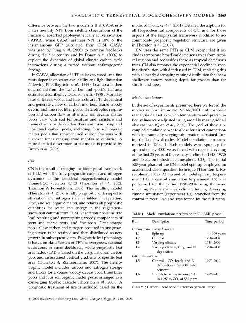
Table 1 Model simulations performed in C-LAMP phase 1

Run Description Time period

Forcing with observed climate

1.1 Spin-up � 4000 years

1.2 Control 1798–2004

1.3 Varying climate 1948–2004

1.4 Varying climate, CO2, and N

deposition

1798–2004

FACE simulations

1.5 Control – CO2 levels and N

deposition after 2004 held

constant

1997–2010

1.6 Branch from Experiment 1.4

in 1997 to CO2 at 550 ppm

1997–2010

C-LAMP, Carbon-LAnd Model Intercomparison Project.



lysis time series from 1948 to 2004. Both experiments 1.2

and 1.3 also had fixed, preindustrial atmospheric CO2.

A second transient simulation (experiment 1.4) started

from the end of model spin up and ran for the period

1798–2004. This simulation had a prescribed, time-vary-

ing atmospheric CO2 time series starting in 1798. For

CN, a nitrogen deposition climatology was used as a

model driver before 1890 followed by a prescribed

nitrogen deposition time series from 1890 to 2004.

Climate forcing in experiment 1.4 was the same as the

control from 1798 to 1947 and as experiment 1.3 from

1948 to 2004. No land use change or dynamic vegetation

simulations were included in this first C-LAMP analy-

sis: land cover was prescribed with preindustrial (year

1798) distributions using the dataset developed by

Feddema et al. (2005). This was done so that future

C-LAMP simulations could branch from this point with

transient land cover change.

The prescribed global atmospheric CO2 time series

was from the C4MIP reconstruction from Friedlingstein

et al. (2006), extended through 2004. The nitrogen de-

position climatology and 1890–2004 time series were

developed as part of the SANTA FE project (Lamarque

et al., 2005). Two additional simulations (experiments

1.5 and 1.6) were designed to test the response of the

models to a sudden increase in atmospheric CO2, fol-

lowing a protocol similar to FACE experiments. These

two latter experiments branched from experiment 1.4 in

1997, with CO2 levels abruptly increasing from 362 to

550 ppm in experiment 1.6. In experiment 1.5, CO2

levels followed atmospheric observations from 1997 to

2004 and then remained constant thereafter at

379.1 ppm. We extended these two simulations to 2010

to explore carbon sink dynamics during the time of

ongoing FACE experiments. More detailed information

about the spin up and simulation protocol is available

in Hoffman et al. (2008) and at http://www.climatemo

deling.org/c-lamp/protocol/protocol.html.

Metadata standards for terrestrial biosphere model

output were developed as part of the C-LAMP protocol.

Proposed as extensions to the netCDF Climate and

Forecast (CF) conventions (Eaton et al., 2008), these

naming conventions will be needed to support output

of model results coming from earth system models

performing simulations for the Intergovernmental

Panel on Climate Change (IPCC) Fifth Assessment

Report (AR5). The proposed extensions are described

at http://www.climatemodeling.org/c-lamp/protocol/

model_output.php. Model results from C-LAMP are

publicly available through the Earth System Grid Cen-

ter for Enabling Technologies (ESG-CET; Ananthakrish-

nan et al., 2007) under the same terms as the database

of physical climate model output used in the IPCC

AR4 (Meehl et al., 2007). The Earth System Grid (ESG;

http://www.earthsystemgrid.org/) is a distributed sys-

tem that allows registered users to download model

output, code, and ancillary data over the Internet

(Bernholdt et al., 2005). A new ESG node has been

deployed at ORNL to support C-LAMP.

Metrics

Multiple sets of observations exist for evaluating terres-

trial biogeochemistry model performance on a range of

temporal and spatial scales (supporting information

Fig. S1). Combining information from these different

data streams to evaluate model performance requires

consideration of the primary objective(s) of the model

simulations, an understanding of the uncertainties as-

sociated with each type of observation, and the degree

to which scaling issues influence the comparison. We

describe below the different observations used in our

analysis.

Leaf area

We compared model estimates with MODerate Resolu-

tion Imaging Spectroradiometer (MODIS) LAI observa-

tions (MOD15A2 collection 4; Myneni et al., 2002) with

additional adjustments to interpolate across periods of

cloud contamination as described by Zhao et al. (2005).

We specifically evaluated the models against three

aspects of the observations: the timing or phase of

maximum LAI (as a diagnostic of seasonality), max-

imum monthly LAI, and annual mean LAI. For the

mean and maximum, biases may exist in the satellite-

derived estimates from errors in atmospheric and ca-

nopy radiative transfer models used in the retrieval.

The metric of the seasonality, based on the month of

maximum LAI, should be less sensitive to these types of

biases, and thus probably has a lower overall level of

uncertainty. In our analysis, we compared 2000–2004

monthly mean MODIS values with model estimates

from experiment 1.4 sampled during the same time

period.

In climate–carbon models, leaf area is a key prognos-

tic variable that couples biophysics, hydrology, and

biogeochemistry. To account for different levels of un-

certainty in our scoring system we gave more weight to

the comparison of LAI phase than to the maximum or

mean. For the phase, we computed the temporal offset

(in months) between model and observations in each

cell, normalized this amount by a maximum possible

offset (6 months), and then averaged this quantity for all

the grid cells in each biome. A quantitative description

of this metric and our scoring approach for LAI is

provided in the supporting information [including

Eqn (s1)]. For the maximum and annual mean LAI



http://www.climatemodeling.org/c-lamp/protocol/protocol.html



http://www.climatemodeling.org/c-lamp/protocol/model_output.php







http://www.earthsystemgrid.org/






comparisons, we estimated the absolute difference be-

tween the model and satellite observations at each grid

cell, normalized this quantity by the sum of model and

observations, and then averaged this quantity for all the

grid cells in a biome [Eqn (s2) in the supporting

information].

NPP

Even though considerable uncertainty exists with field-

based measurement approaches, we included NPP as

one of our metrics because it is a fundamental quantity

that determines the availability of food, fuel, and fiber

resources for humans. It also regulates carbon storage in

long-lived pools (such as wood) that, in turn, deter-

mines the magnitude of terrestrial sinks and sources in

response to various drivers of global change. We used

two data sources for our comparisons: compilations of

NPP observations from the Ecosystem Model Data

Intercomparison (EMDI) (Olson et al., 2001) and spatial

patterns of NPP derived using MODIS satellite observa-

tions (Zhao et al., 2005, 2006). To extract information

from these two datasets, we designed four different

comparisons. Using the EMDI observations, we made

(1) point-by-point comparisons of observations and

corresponding model grid cells and (2) histograms of

NPP vs. precipitation for both the observations and the

models. We evaluated model performance using Eqn

(s2) in the supporting information in grid cells where

EMDI observations were available. Separate compari-

sons were made for EMDI observations classified as

high quality (81 sites; class A) and intermediate quality

(933 sites; class B). NPP observations were compared

with mean annual NPP averaged during 1975–2000

from experiment 1.4.

A large mismatch in spatial scale between the site-

level EMDI observations and the size of an individual

model grid cell probably compromises the value of this

dataset for evaluating model performance. In contrast,

MODIS NPP estimates are based on high resolution

(1 km) satellite measurements of the fAPAR across the

entire domain of a model grid cell, potentially limiting

errors associated with scaling. Here we used the

MOD17A3 collection 4.5 product (Heinsch et al., 2003).

Biases could exist, however, in MODIS NPP if there are

errors associated with the underlying algorithms that

convert satellite radiances to fAPAR or with the con-

version of APAR to NPP using a light use efficiency

model. To try to avoid these biases in our scoring

system (but still maintaining access to the rich spatial

information from the satellite observations), we com-

puted the square of the Pearson correlation coefficient

(r2) between MODIS NPP and the models using all

model grid cells and, separately, using the latitudinal

zonal means.

The annual cycle of atmospheric carbon dioxide

Measurements of the annual cycle of atmospheric CO2

from NOAA’s Global Monitoring Division (GMD) and

other networks (Globalview; Masarie & Tans, 1995)

provide a means to evaluate model fluxes of monthly

NEE for biomes in the northern part of the northern

hemisphere. Seasonal NEE fluxes are controlled by both

the magnitude and timing of NPP and the temperature

sensitivity of heterotrophic respiration (Kaminski et al.,

2002; Randerson et al., 2002). Measurements of the

annual cycle are a robust constraint at a large spatial

scale on the combined set of processes regulating NEE

because (1) ocean and fossil fuel fluxes contribute only

weakly to seasonal variations in CO2 in the northern

hemisphere (Randerson et al., 1997; Heimann et al., 1998;

Nevison et al., 2008) and (2) the CO2 measurements are

precise (Conway et al., 1994). These data-model com-

parisons are sensitive, however, to biases in the atmo-

spheric model–particularly with respect to convection,

planetary boundary layer mixing, and other processes

that regulate vertical mixing (Stephens et al., 2007; Yang

et al., 2007).

To compare with the Globalview observations, we

combined CASA0 and CN surface CO2 fluxes with

monthly atmospheric impulse functions from the At-

mospheric Tracer Transport Model Intercomparison

Project (TRANSCOM) phase 3 level 2 experiments

(Gurney et al., 2004) to construct simulated annual

cycles of atmospheric CO2. Using techniques applied

in interannual inversions, the response functions were

used to fill a matrix (the H matrix defined in Baker et al.,

2006). Monthly NEE fluxes from CASA0 and CN 1.4

experiments for 1988–2000 were aggregated within each

of the 11 TRANSCOM land basis regions. The aggre-

gated fluxes were multiplied by the H matrix to con-

struct modeled 1991–2000 interannual CO2 mixing time

series at observation stations. We computed an annual

cycle for each of the 13 TRANSCOM atmospheric

models and report the model mean. For our scoring

system, we estimated model performance in three dif-

ferent latitude bands in the northern hemisphere. We

computed the square of the Pearson correlation coeffi-

cient (as a metric of phase) and the ratio of model to

observed amplitudes (as a metric of magnitude) for

each Globalview station. Each station was weighted

equally in constructing the zonal means. We assigned

a higher number of possible points to the 90–601N and

30–601N latitude zones than to the EQ – 301N band

because the signal to noise ratio of the observed annual

cycle is higher at mid and high latitudes and because



the contribution in these bands from other fluxes (from

ocean and fossil fuel fluxes) is substantially lower.

Eddy covariance measurements of energy and carbon

Eddy covariance measurements provide a powerful

constraint on surface energy exchange (Stockli et al.,

2008), the seasonal dynamics of NEE (Falge et al., 2002)

and GPP (Falge et al., 2002; Heinsch et al., 2006). Prog-

nostic leaf area from the biogeochemical model must be

integrated with other aspects of the LSM to predict, for

example, the flow of available energy into latent and

sensible heat. Here we compared the models with

available gap-filled Ameriflux level 4 data (http://public.

ornl.gov/ameriflux/available.shtml). We made specific

comparisons against monthly mean fluxes of (1) NEE,

(2) GPP, (3) latent heat, and (4) sensible heat. We

sampled the model grid cells (from experiment 1.4)

during each year that the observations were available

to build a multiyear set of mean monthly fluxes through

2004. We estimated model-data agreement using Eqn

(s2) in the supporting information at each site using the

monthly means, and weighted information from each

site equally in constructing our overall score. We as-

signed fewer scoring points to the GPP and NEE

comparisons based on a subjective assessment that

these fluxes had higher measurement and scaling un-

certainties, respectively, than concurrent latent and

sensible heat fluxes (see text in supporting information).

We present specific site-level comparisons for Sylva-

nia Wilderness (Desai et al., 2005), Harvard Forest

(Barford et al., 2001), and Walker Branch (Wilson &

Baldocchi, 2001). For our overall scoring system, how-

ever, we used information for each variable from all

available Ameriflux sites. This included information

from 74 sites, ranging from arctic tundra at Atqasuk

(701N) to pine forests at the Kennedy Space Center

(281N). A primary source of uncertainty in the model-

data comparison for eddy covariance observations is

the spatial scale mismatch. This may be improved in

future by forcing the models directly with site-level

climate observations and with PFT distributions that

match the observed distribution within the tower foot-

print (e.g., Stockli et al., 2008).

Aboveground biomass stocks and fluxes

Aboveground carbon in contemporary forests is a large

and vulnerable carbon pool that is sensitive to both land

use and climate change. The size of this pool is one of

the primary uncertainties associated with estimates of

contemporary carbon loss from deforestation. Within

the Amazon basin, considerable effort has gone into

developing methods to measure and extrapolate forest

biomass to basin-wide inventories (Fearnside, 1992;

Houghton et al., 2001). In Brazil’s Amazonian forests,

estimates of total live and dead biomass (including

coarse roots) range between 39 and 93 Pg C, with a mean

and standard error of 70 � 8 Pg C (Houghton et al., 2001).

To compare with model estimates, we used the map of

contemporary (ca. 2000) aboveground live biomass

developed by Saatchi et al. (2007). This map was devel-

oped using 540 plot measurements of biomass, includ-

ing the 44 measurements summarized by Houghton

et al. (2001), and a decision tree classification approach

based on multiple satellite data sets. Within the Amazon

basin, mean forest biomass (including live, dead, and

belowground wood) was 158 Mg C ha�1 for a total of

86 Pg C within the study domain of 5.46� 106 km2

(Saatchi et al., 2007). For our scoring metric we used

Eqn (s2) in the supporting information. We specifically

compared model output for the year 2000 from experi-

ment 1.4 with the observations at each grid cell.

Sensitivity of NPP to increasing levels ofatmospheric CO2

To characterize the sensitivity of model NPP to elevated

levels of CO2 we performed two model simulations

described above (experiments 1.5 and 1.6) to mimic

control and treatment plots in FACE experiments. We

made a direct comparison of temperate forest grid cell

NPP increases with site level averages from Norby et al.

(2005) – estimating the percent increases in NPP sepa-

rately for grid cells corresponding to each of the four

FACE sites. The model-data differences for the four sites

were used with Eqn (s2) in the supporting information

to generate a scoring metric. We also report the zonal

mean responses of the two models.

We computed the biotic growth factor, bfert, as:

bfert ¼ðNPPf �NPPiÞ=NPPf

lnðCf=CiÞð1Þ

where NPPi was the mean NPP from the control during

1997–2001 (exp. 1.5) and NPPf was the mean NPP from

the FACE simulation (exp. 1.6) for this same period.

Ci and Cf were the control (�365 ppm) and FACE

(550 ppm) atmospheric CO2 mixing ratios.

Interannual variability in carbon fluxes

We compared model estimates of interannual variabil-

ity in NEE with flux estimates from TRANSCOM (Baker

et al., 2006). The TRANSCOM fluxes were obtained

using Globalview CO2 measurements and the same

impulse–response functions described above. The

inversion was based on observations from 78 flask



http://public.ornl.gov/ameriflux/available.shtml

















stations and a Bayesian approach with seasonally vary-

ing a priori uncertainties for land regions, time-invariant

prior uncertainties for the ocean, and a diagonal error

covariance matrix which was comprised of the variance

of the observations measured at each station. Fluxes

from Baker et al. (2006) spanned the 1988–2003 period.

For comparison with C-LAMP models, they were ex-

tended by Baker through 2004 using the same station

network and inversion approach (D. Baker, personal

communication, March 2008). Our scoring metric com-

bined information about (1) the correlation between the

global annual mean model fluxes and the observations

during 1988–2004 and (2) the magnitude of model

variability as compared with that in the observations.

Fire emissions were assessed by comparing CN with

the Global Fire Emissions Database version 2 (GFEDv2)

(van der Werf et al., 2006). The version of CASA0

evaluated here did not predict fires. GFEDv2 estimates

of burned area were constructed by combining MODIS

active fire observations with MODIS burned area tiles

(where available) using a regression tree approach

(Giglio et al., 2006). We used Eqn (s2) in the supporting

information with globally averaged monthly fluxes

during 1997–2004 to estimate model performance.

We note that both the TRANSCOM and GFEDv2

fluxes were obtained using models as key intermediary

steps in transforming raw observations to fluxes. Un-

certainties in these models – including biases in atmo-

spheric transport for TRANSCOM and biases in fuel

loads and combustion completeness for GFEDv2 are

difficult to quantify. As a result, the total number of

points we assigned to these comparisons in our scoring

system was lower than for other classes of constraints in

the transient dynamics section. We expect the quality of

both these time series to improve in future with new

satellite observations (e.g., Crisp et al., 2004) and data

assimilation systems.

Results

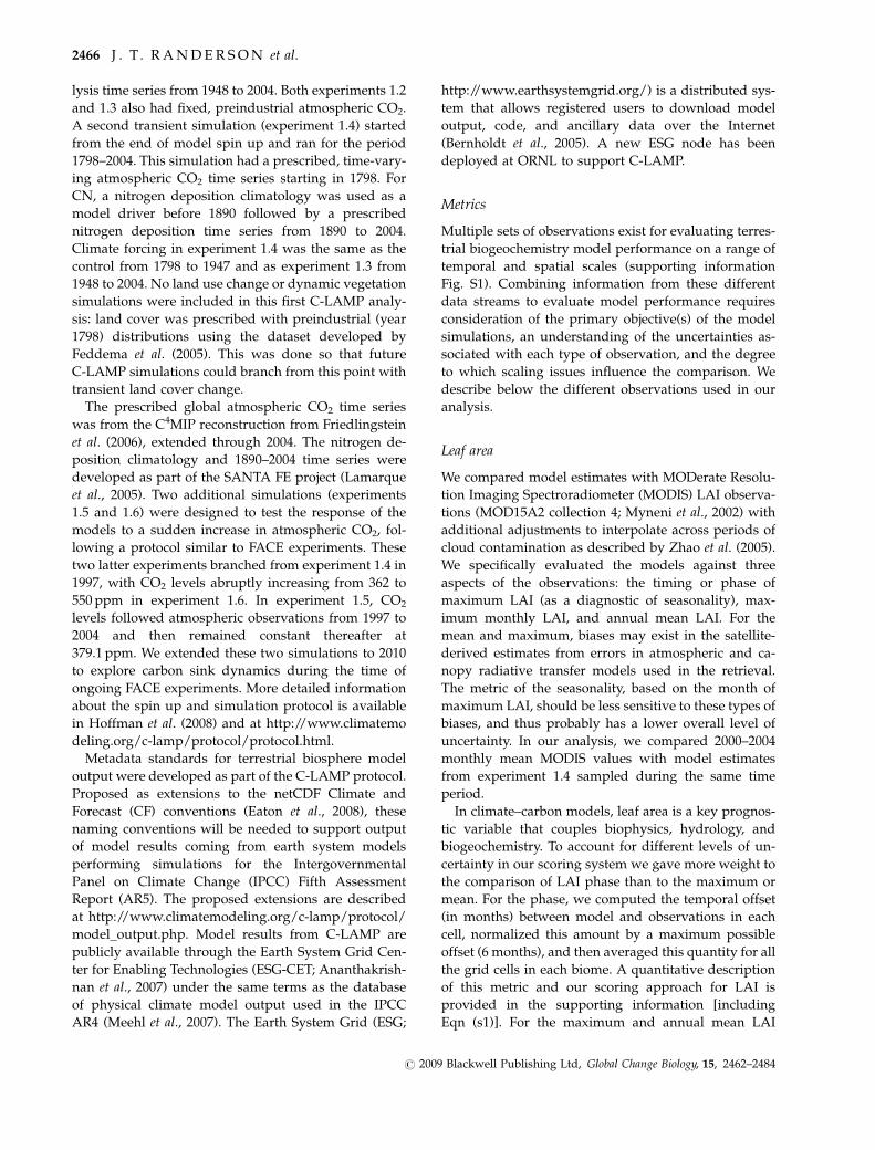
Comparison with MODIS LAI showed that for both

models, the timing of maximum leaf area lagged behind

the observations by 1–2 months (Fig. 1). In many boreal

and arctic ecosystems, for example, maximum observed

LAI occurred in July, whereas in the models the max-

imum occurred in August (CASA0) or September (CN).

These lags also occurred in moisture-limited savanna

ecosystems, although CN matched observed patterns

reasonably well in southern hemisphere South America

and CASA0 performed reasonably well in Africa. The

systematic nature of these timing delays suggests that

the prognostic leaf area schemes for both models may

underestimate carryover pools of carbohydrates from

one growing season to the next – and thus the potential

for rapid leaf expansion at the onset of the growing

season. For other aspects of LAI, including mean and

maximum levels, the models performed reasonably well

in most biomes (data not shown). One exception was

that LAI was low in CN in many boreal and arctic

regions. This bias was partly a consequence of the

coupling to the hydrology model that did not adequately

capture freeze-thaw dynamics (Lawrence et al., 2007).

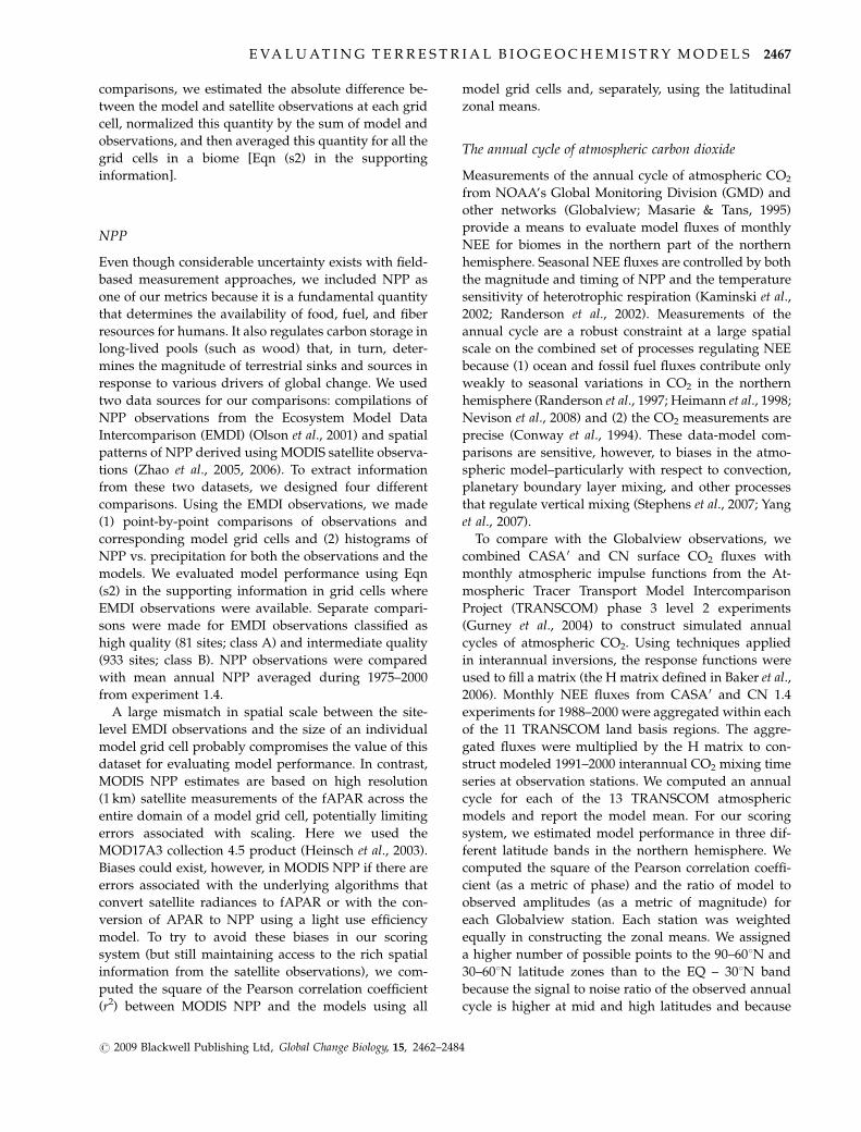
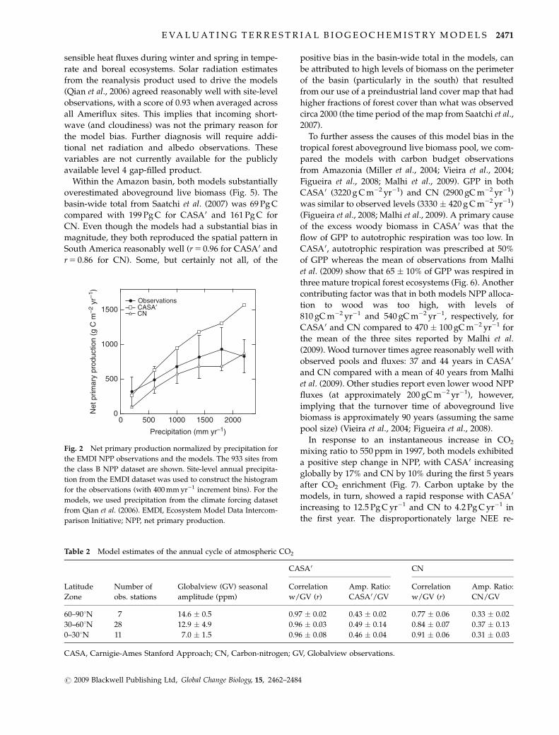
Direct comparison with EMDI site-level NPP showed

that CASA0 was higher than the observations in inter-

mediate and high productivity areas, whereas CN was

lower than the observations in low productivity areas

(supporting information Fig. S2). This pattern of bias

remained the same when the models were compared as

a function of precipitation level (Fig. 2) and latitude

(supporting information Fig. S3). Specifically, CASA0

had a high bias in high precipitation and tropical areas,

whereas CN had a low bias of similar relative magni-

tude in boreal and arctic ecosystems.

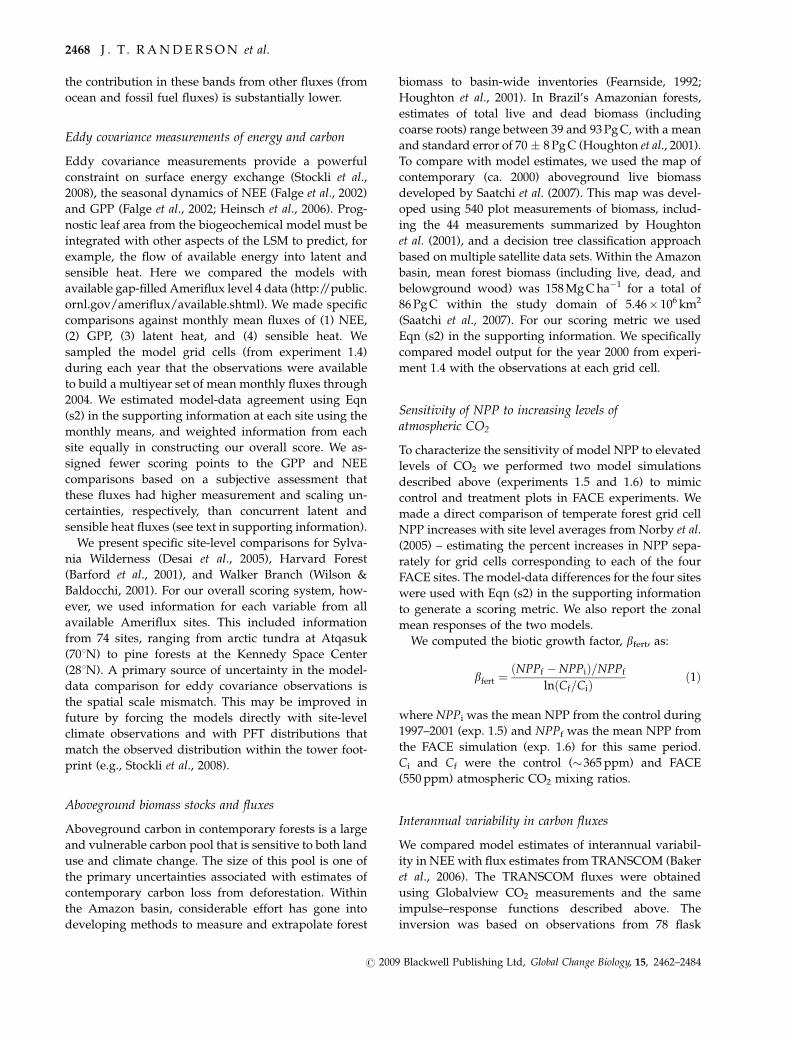
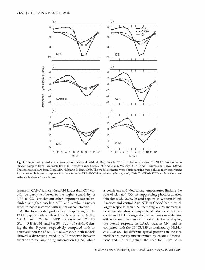
Both models substantially underestimated the seaso-

nal amplitude of CO2 in the northern hemisphere –

CASA0 by a factor of �2 and CN by a factor �3 (Table 2).

CN also had a phase offset with the observations, with

drawdown of CO2 in spring occurring 1–3 months

earlier than in the observations (Fig. 3). For CASA0 the

smaller amplitude was probably caused by either a

temperature sensitivity of heterotrophic respiration

(e.g., a Q10 factor) that was too high in northern eco-

systems or a seasonal distribution of NPP that was not

concentrated enough during the middle part of the

growing season. In contrast, for CN the low NPP in

ecosystems north of 401N (supporting information Fig.

S3) also reduced the magnitude of heterotrophic re-

spiration and thus the magnitude of seasonal variations

in NEP.

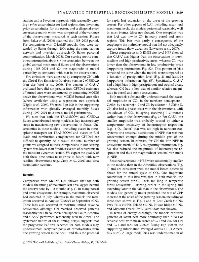
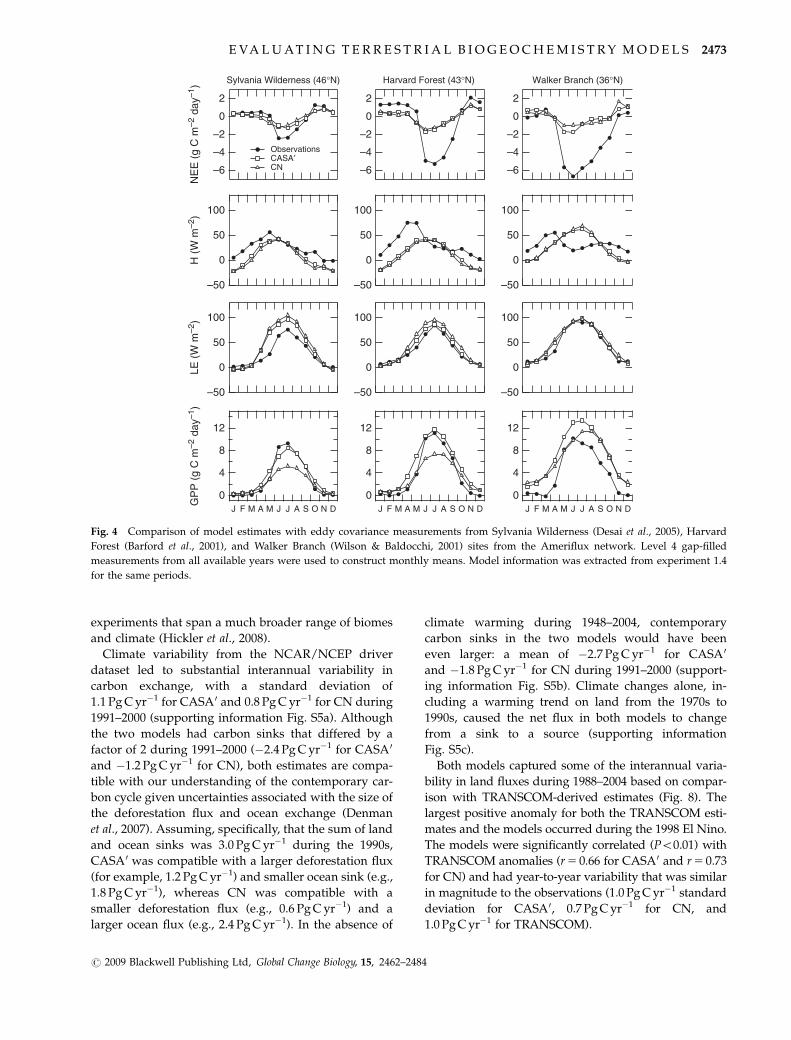
Seasonal variations in NEE were substantially smaller

in the models than in the Ameriflux observations (Fig.

4) and are consistent with the model biases described

above for the annual cycle of CO2. One important

contributor to this bias was that in both models, the

growing season for GPP was too long in temperate

forest ecosystems – starting earlier in the spring and

extending later in the fall than in the observations. The

models also generally under predicted the rate of GPP

increase at the onset of the growing season, including at

three sites shown in Fig. 4 and at Lost Creek (461N),

Park Falls (461N), Toledo (421N), Niwot Ridge (401N),

and Missouri Ozark (391N) sites (data not shown).

In terms of energy exchange, the models captured

patterns of latent heat more accurately than fluxes of

sensible heat, with mean scores of 0.71 and 0.52 for CN

and 0.71 and 0.54 for CASA0 [using Eqn (s2) in the

supporting information averaged across all L4 Ameri-

flux sites]. A large model bias was underestimation of



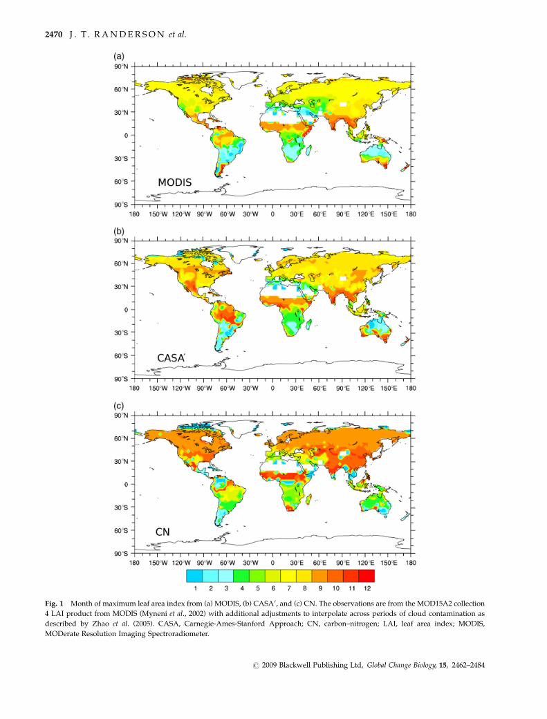
Fig. 1 Month of maximum leaf area index from (a) MODIS, (b) CASA0, and (c) CN. The observations are from the MOD15A2 collection

4 LAI product from MODIS (Myneni et al., 2002) with additional adjustments to interpolate across periods of cloud contamination as

described by Zhao et al. (2005). CASA, Carnegie-Ames-Stanford Approach; CN, carbon–nitrogen; LAI, leaf area index; MODIS,

MODerate Resolution Imaging Spectroradiometer.



sensible heat fluxes during winter and spring in tempe-

rate and boreal ecosystems. Solar radiation estimates

from the reanalysis product used to drive the models

(Qian et al., 2006) agreed reasonably well with site-level

observations, with a score of 0.93 when averaged across

all Ameriflux sites. This implies that incoming short-

wave (and cloudiness) was not the primary reason for

the model bias. Further diagnosis will require addi-

tional net radiation and albedo observations. These

variables are not currently available for the publicly

available level 4 gap-filled product.

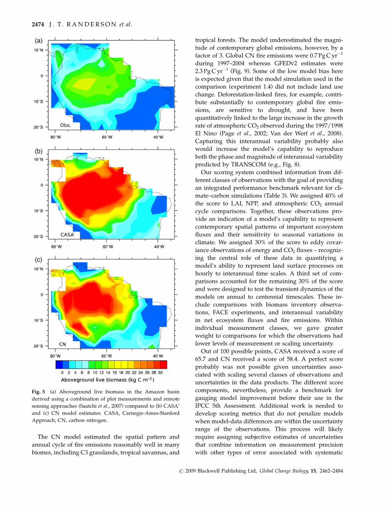
Within the Amazon basin, both models substantially

overestimated aboveground live biomass (Fig. 5). The

basin-wide total from Saatchi et al. (2007) was 69 Pg C

compared with 199 Pg C for CASA0 and 161 Pg C for

CN. Even though the models had a substantial bias in

magnitude, they both reproduced the spatial pattern in

South America reasonably well (r 5 0.96 for CASA0 and

r 5 0.86 for CN). Some, but certainly not all, of the

positive bias in the basin-wide total in the models, can

be attributed to high levels of biomass on the perimeter

of the basin (particularly in the south) that resulted

from our use of a preindustrial land cover map that had

higher fractions of forest cover than what was observed

circa 2000 (the time period of the map from Saatchi et al.,

2007).

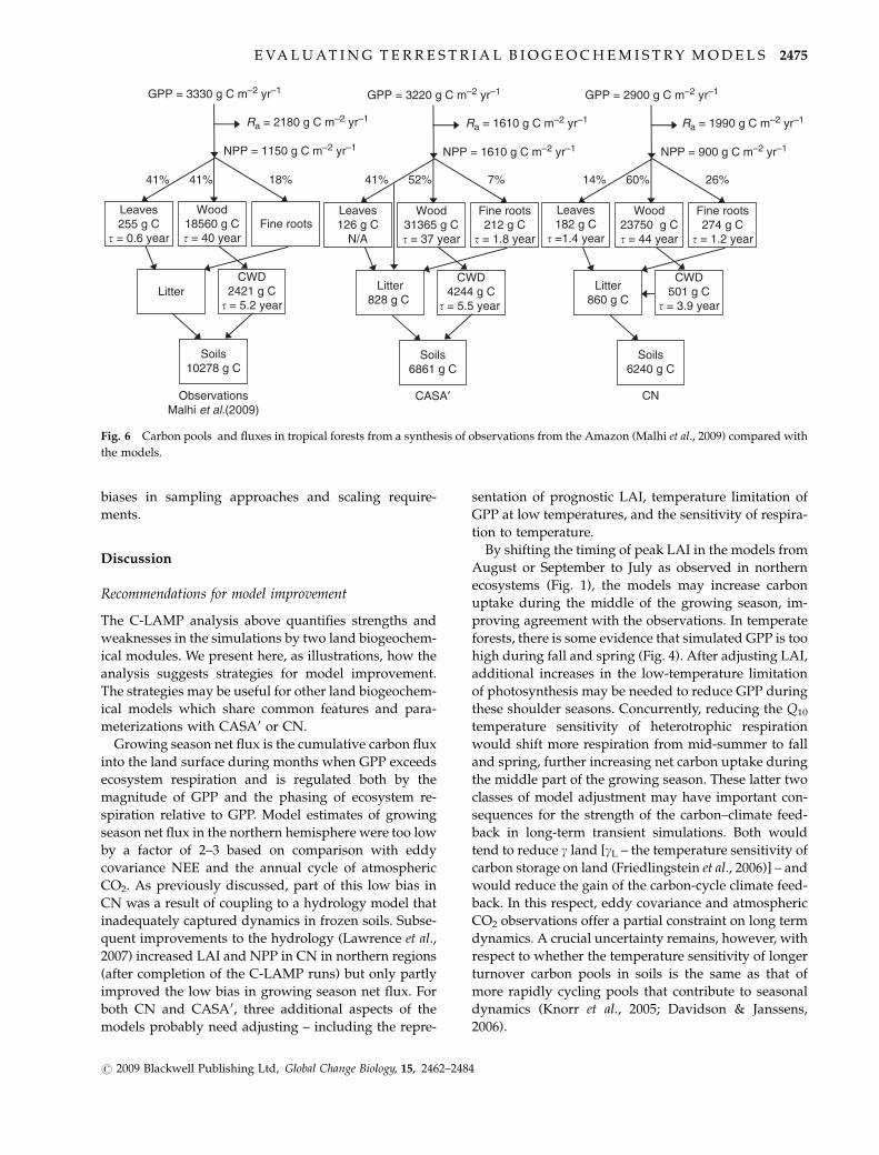
To further assess the causes of this model bias in the

tropical forest aboveground live biomass pool, we com-

pared the models with carbon budget observations

from Amazonia (Miller et al., 2004; Vieira et al., 2004;

Figueira et al., 2008; Malhi et al., 2009). GPP in both

CASA0 (3220 g C m�2 yr�1) and CN (2900 gC m�2 yr�1)

was similar to observed levels (3330 � 420 g C m�2 yr�1)

(Figueira et al., 2008; Malhi et al., 2009). A primary cause

of the excess woody biomass in CASA0 was that the

flow of GPP to autotrophic respiration was too low. In

CASA0, autotrophic respiration was prescribed at 50%

of GPP whereas the mean of observations from Malhi

et al. (2009) show that 65 � 10% of GPP was respired in

three mature tropical forest ecosystems (Fig. 6). Another

contributing factor was that in both models NPP alloca-

tion to wood was too high, with levels of

810 gC m�2 yr�1 and 540 gC m�2 yr�1, respectively, for

CASA0 and CN compared to 470 � 100 gC m�2 yr�1 for

the mean of the three sites reported by Malhi et al.

(2009). Wood turnover times agree reasonably well with

observed pools and fluxes: 37 and 44 years in CASA0

and CN compared with a mean of 40 years from Malhi

et al. (2009). Other studies report even lower wood NPP

fluxes (at approximately 200 gC m�2 yr�1), however,

implying that the turnover time of aboveground live

biomass is approximately 90 years (assuming the same

pool size) (Vieira et al., 2004; Figueira et al., 2008).

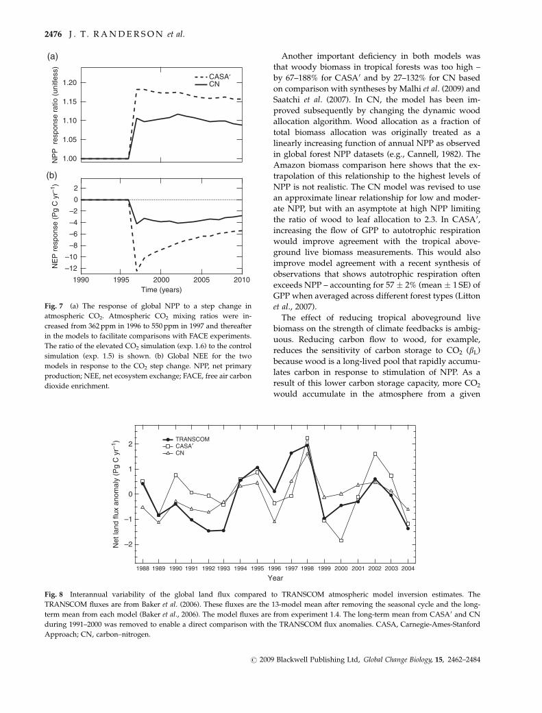
In response to an instantaneous increase in CO2

mixing ratio to 550 ppm in 1997, both models exhibited

a positive step change in NPP, with CASA0 increasing

globally by 17% and CN by 10% during the first 5 years

after CO2 enrichment (Fig. 7). Carbon uptake by the

models, in turn, showed a rapid response with CASA0

increasing to 12.5 Pg C yr�1 and CN to 4.2 Pg C yr�1 in

the first year. The disproportionately large NEE re-

1500

1000

500

02000150010005000

ObservationsCASA′CN

Precipitation (mm yr–1)

Net

prim

ary

prod

uctio

n (g

C m

–2 y

r–1)

Fig. 2 Net primary production normalized by precipitation for

the EMDI NPP observations and the models. The 933 sites from

the class B NPP dataset are shown. Site-level annual precipita-

tion from the EMDI dataset was used to construct the histogram

for the observations (with 400 mm yr�1 increment bins). For the

models, we used precipitation from the climate forcing dataset

from Qian et al. (2006). EMDI, Ecosystem Model Data Intercom-

parison Initiative; NPP, net primary production.

Table 2 Model estimates of the annual cycle of atmospheric CO2

Latitude

Zone

Number of

obs. stations

Globalview (GV) seasonal

amplitude (ppm)

CASA0 CN

Correlation

w/GV (r)

Amp. Ratio:

CASA0/GV

Correlation

w/GV (r)

Amp. Ratio:

CN/GV

60–901N 7 14.6 � 0.5 0.97 � 0.02 0.43 � 0.02 0.77 � 0.06 0.33 � 0.02

30–601N 28 12.9 � 4.9 0.96 � 0.03 0.49 � 0.14 0.84 � 0.07 0.37 � 0.13

0–301N 11 7.0 � 1.5 0.96 � 0.08 0.46 � 0.04 0.91 � 0.06 0.31 � 0.03

CASA, Carnigie-Ames Stanford Approach; CN, Carbon-nitrogen; GV, Globalview observations.



sponse in CASA0 (almost threefold larger than CN) can

only be partly attributed to the higher sensitivity of

NPP to CO2 enrichment; other important factors in-

cluded a higher baseline NPP and similar turnover

times in pools involved with initial carbon storage.

At the four model grid cells corresponding to the

FACE experiments analyzed by Norby et al. (2005),

CASA0 and CN had NPP increases of 17 � 2%

(bfert 5 0.43 � 0.04) and 7 � 3% (bfert 5 0.18 � 0.09) dur-

ing the first 5 years, respectively, compared with an

observed increase of 27 � 2% (bfert 5 0.67). Both models

showed a decreasing trend in NPP response between

401N and 701N (supporting information Fig. S4) which

is consistent with decreasing temperatures limiting the

role of elevated CO2 in suppressing photorespiration

(Hickler et al., 2008). In arid regions in western North

America and central Asia NPP in CASA0 had a much

larger response than CN, including a 28% increase in

broadleaf deciduous temperate shrubs vs. a 12% in-

crease in CN. This suggests that increases in water use

efficiency may be a more important factor in shaping

the overall response in CASA0 than in CN (and as

compared with the LPJ-GUESS as analyzed by Hickler

et al., 2008). The different spatial patterns in the two

models are mostly unconstrained by existing observa-

tions and further highlight the need for future FACE

Month Month

Det

rend

ed C

O2

mix

ing

ratio

(pp

m)

MBC ICE

CARR 6K AZR

MID KUM–6

–4

–2

0

2

4

121110987654321

–6

–4

–2

0

2

4

121110987654321

–6

–4

–2

0

2

4

–6

–4

–2

0

2

4

–10

–5

0

5 Obs.CASA′CN

–10

–5

0

5

(a) (b)

(c) (d)

(e) (f)

Fig. 3 The annual cycle of atmospheric carbon dioxide at (a) Mould Bay, Canada (761N), (b) Storhofdi, Iceland (631N), (c) Carr, Colorado

(aircraft samples from 6 km masl; 411N), (d) Azores Islands (391N), (e) Sand Island, Midway (281N), and (f) Kumakahi, Hawaii (201N).

The observations are from Globalview (Masarie & Tans, 1995). The model estimates were obtained using model fluxes from experiment

1.4 and monthly impulse response functions from the TRANSCOM experiment (Gurney et al., 2004). The TRANSCOM multimodel mean

estimate is shown for each case.



experiments that span a much broader range of biomes

and climate (Hickler et al., 2008).

Climate variability from the NCAR/NCEP driver

dataset led to substantial interannual variability in

carbon exchange, with a standard deviation of

1.1 Pg C yr�1 for CASA0 and 0.8 Pg C yr�1 for CN during

1991–2000 (supporting information Fig. S5a). Although

the two models had carbon sinks that differed by a

factor of 2 during 1991–2000 (�2.4 Pg C yr�1 for CASA0

and �1.2 Pg C yr�1 for CN), both estimates are compa-

tible with our understanding of the contemporary car-

bon cycle given uncertainties associated with the size of

the deforestation flux and ocean exchange (Denman

et al., 2007). Assuming, specifically, that the sum of land

and ocean sinks was 3.0 Pg C yr�1 during the 1990s,

CASA0 was compatible with a larger deforestation flux

(for example, 1.2 Pg C yr�1) and smaller ocean sink (e.g.,

1.8 Pg C yr�1), whereas CN was compatible with a

smaller deforestation flux (e.g., 0.6 Pg C yr�1) and a

larger ocean flux (e.g., 2.4 Pg C yr�1). In the absence of

climate warming during 1948–2004, contemporary

carbon sinks in the two models would have been

even larger: a mean of �2.7 Pg C yr�1 for CASA0

and �1.8 Pg C yr�1 for CN during 1991–2000 (support-

ing information Fig. S5b). Climate changes alone, in-

cluding a warming trend on land from the 1970s to

1990s, caused the net flux in both models to change

from a sink to a source (supporting information

Fig. S5c).

Both models captured some of the interannual varia-

bility in land fluxes during 1988–2004 based on compar-

ison with TRANSCOM-derived estimates (Fig. 8). The

largest positive anomaly for both the TRANSCOM esti-

mates and the models occurred during the 1998 El Nino.

The models were significantly correlated (Po0.01) with

TRANSCOM anomalies (r 5 0.66 for CASA0 and r 5 0.73

for CN) and had year-to-year variability that was similar

in magnitude to the observations (1.0 Pg C yr�1 standard

deviation for CASA0, 0.7 Pg C yr�1 for CN, and

1.0 Pg C yr�1 for TRANSCOM).

Sylvania Wilderness (46°N) Walker Branch (36°N)

GP

P (

g C

m–2

day

–1)

LE (

W m

–2)

H (

W m

–2)

NE

E (

g C

m–2

day

–1)

–6

–4

–2

0

2

12

8

4

0

100

50

0

–50

100

50

0

–50

100

50

0

–50

100

50

0

–50

12

8

4

0

–6

–4

–2

0

2

12

8

4

0

100

50

0

–50

100

50

0

–50

–6

–4

–2

0

2

ObservationsCASA′CN

DNOSAA MM JJJ FDNOSAA MM JJJ FDNOSAA MM JJJ F

Harvard Forest (43°N)

Fig. 4 Comparison of model estimates with eddy covariance measurements from Sylvania Wilderness (Desai et al., 2005), Harvard

Forest (Barford et al., 2001), and Walker Branch (Wilson & Baldocchi, 2001) sites from the Ameriflux network. Level 4 gap-filled

measurements from all available years were used to construct monthly means. Model information was extracted from experiment 1.4

for the same periods.



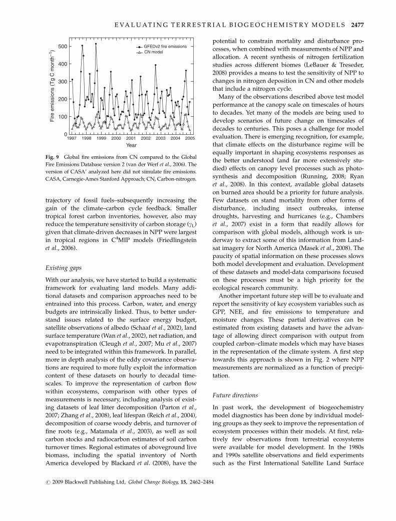
The CN model estimated the spatial pattern and

annual cycle of fire emissions reasonably well in many

biomes, including C3 grasslands, tropical savannas, and

tropical forests. The model underestimated the magni-

tude of contemporary global emissions, however, by a

factor of 3. Global CN fire emissions were 0.7 Pg C yr�1

during 1997–2004 whereas GFEDv2 estimates were

2.3 Pg C yr�1 (Fig. 9). Some of the low model bias here

is expected given that the model simulation used in the

comparison (experiment 1.4) did not include land use

change. Deforestation-linked fires, for example, contri-

bute substantially to contemporary global fire emis-

sions, are sensitive to drought, and have been

quantitatively linked to the large increase in the growth

rate of atmospheric CO2 observed during the 1997/1998

El Nino (Page et al., 2002; Van der Werf et al., 2008).

Capturing this interannual variability probably also

would increase the model’s capability to reproduce

both the phase and magnitude of interannual variability

predicted by TRANSCOM (e.g., Fig. 8).

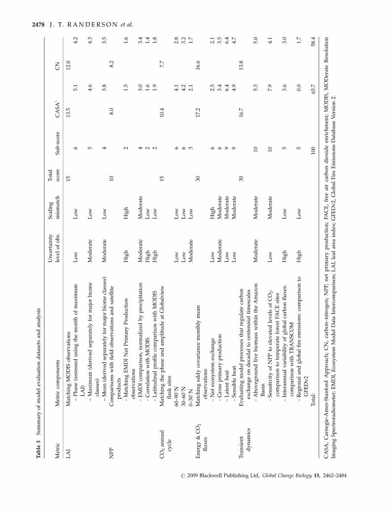
Our scoring system combined information from dif-

ferent classes of observations with the goal of providing

an integrated performance benchmark relevant for cli-

mate–carbon simulations (Table 3). We assigned 40% of

the score to LAI, NPP, and atmospheric CO2 annual

cycle comparisons. Together, these observations pro-

vide an indication of a model’s capability to represent

contemporary spatial patterns of important ecosystem

fluxes and their sensitivity to seasonal variations in

climate. We assigned 30% of the score to eddy covar-

iance observations of energy and CO2 fluxes – recogniz-

ing the central role of these data in quantifying a

model’s ability to represent land surface processes on

hourly to interannual time scales. A third set of com-

parisons accounted for the remaining 30% of the score

and were designed to test the transient dynamics of the

models on annual to centennial timescales. These in-

clude comparisons with biomass inventory observa-

tions, FACE experiments, and interannual variability

in net ecosystem fluxes and fire emissions. Within

individual measurement classes, we gave greater

weight to comparisons for which the observations had

lower levels of measurement or scaling uncertainty.

Out of 100 possible points, CASA received a score of

65.7 and CN received a score of 58.4. A perfect score

probably was not possible given uncertainties asso-

ciated with scaling several classes of observations and

uncertainties in the data products. The different score

components, nevertheless, provide a benchmark for

gauging model improvement before their use in the

IPCC 5th Assessment. Additional work is needed to

develop scoring metrics that do not penalize models

when model-data differences are within the uncertainty

range of the observations. This process will likely

require assigning subjective estimates of uncertainties

that combine information on measurement precision

with other types of error associated with systematic

Fig. 5 (a) Aboveground live biomass in the Amazon basin

derived using a combination of plot measurements and remote

sensing approaches (Saatchi et al., 2007) compared to (b) CASA0

and (c) CN model estimates. CASA, Carnegie-Ames-Stanford

Approach; CN, carbon–nitrogen.



biases in sampling approaches and scaling require-

ments.

Discussion

Recommendations for model improvement

The C-LAMP analysis above quantifies strengths and

weaknesses in the simulations by two land biogeochem-

ical modules. We present here, as illustrations, how the

analysis suggests strategies for model improvement.

The strategies may be useful for other land biogeochem-

ical models which share common features and para-

meterizations with CASA0 or CN.

Growing season net flux is the cumulative carbon flux

into the land surface during months when GPP exceeds

ecosystem respiration and is regulated both by the

magnitude of GPP and the phasing of ecosystem re-

spiration relative to GPP. Model estimates of growing

season net flux in the northern hemisphere were too low

by a factor of 2–3 based on comparison with eddy

covariance NEE and the annual cycle of atmospheric

CO2. As previously discussed, part of this low bias in

CN was a result of coupling to a hydrology model that

inadequately captured dynamics in frozen soils. Subse-

quent improvements to the hydrology (Lawrence et al.,

2007) increased LAI and NPP in CN in northern regions

(after completion of the C-LAMP runs) but only partly

improved the low bias in growing season net flux. For

both CN and CASA0, three additional aspects of the

models probably need adjusting – including the repre-

sentation of prognostic LAI, temperature limitation of

GPP at low temperatures, and the sensitivity of respira-

tion to temperature.

By shifting the timing of peak LAI in the models from

August or September to July as observed in northern

ecosystems (Fig. 1), the models may increase carbon

uptake during the middle of the growing season, im-

proving agreement with the observations. In temperate

forests, there is some evidence that simulated GPP is too

high during fall and spring (Fig. 4). After adjusting LAI,

additional increases in the low-temperature limitation

of photosynthesis may be needed to reduce GPP during

these shoulder seasons. Concurrently, reducing the Q10

temperature sensitivity of heterotrophic respiration

would shift more respiration from mid-summer to fall

and spring, further increasing net carbon uptake during

the middle part of the growing season. These latter two

classes of model adjustment may have important con-

sequences for the strength of the carbon–climate feed-

back in long-term transient simulations. Both would

tend to reduce g land [gL – the temperature sensitivity of

carbon storage on land (Friedlingstein et al., 2006)] – and

would reduce the gain of the carbon-cycle climate feed-

back. In this respect, eddy covariance and atmospheric

CO2 observations offer a partial constraint on long term

dynamics. A crucial uncertainty remains, however, with

respect to whether the temperature sensitivity of longer

turnover carbon pools in soils is the same as that of

more rapidly cycling pools that contribute to seasonal

dynamics (Knorr et al., 2005; Davidson & Janssens,

2006).

GPP = 2900 g C m–2 yr–1

NPP = 900 g C m–2 yr–1

Ra = 1990 g C m–2 yr–1

Leaves182 g C

� =1.4 year

Wood23750 g C� = 44 year

Fine roots274 g C

� = 1.2 year

Soils6240 g C

Litter860 g C

CWD501 g C

� = 3.9 year

GPP = 3220 g C m–2 yr–1

NPP = 1610 g C m–2 yr–1

Ra = 1610 g C m–2 yr–1

Leaves126 g C

N/A


Fine roots212 g C

� = 1.8 year

Soils6861 g C

Litter828 g C

CWD4244 g C

� = 5.5 year

GPP = 3330 g C m–2 yr–1

NPP = 1150 g C m–2 yr–1

Ra = 2180 g C m–2 yr–1

Leaves255 g C

� = 0.6 year


Fine roots

Soils10278 g C

LitterCWD

2421 g C� = 5.2 year

ObservationsMalhi et al.(2009)

CASA′ CN

41% 41% 18% 14% 60% 26%41% 52% 7%

Fig. 6 Carbon pools and fluxes in tropical forests from a synthesis of observations from the Amazon (Malhi et al., 2009) compared with

the models.



Another important deficiency in both models was

that woody biomass in tropical forests was too high –

by 67–188% for CASA0 and by 27–132% for CN based

on comparison with syntheses by Malhi et al. (2009) and

Saatchi et al. (2007). In CN, the model has been im-

proved subsequently by changing the dynamic wood

allocation algorithm. Wood allocation as a fraction of

total biomass allocation was originally treated as a

linearly increasing function of annual NPP as observed

in global forest NPP datasets (e.g., Cannell, 1982). The

Amazon biomass comparison here shows that the ex-

trapolation of this relationship to the highest levels of

NPP is not realistic. The CN model was revised to use

an approximate linear relationship for low and moder-

ate NPP, but with an asymptote at high NPP limiting

the ratio of wood to leaf allocation to 2.3. In CASA0,

increasing the flow of GPP to autotrophic respiration

would improve agreement with the tropical above-

ground live biomass measurements. This would also

improve model agreement with a recent synthesis of

observations that shows autotrophic respiration often

exceeds NPP – accounting for 57 � 2% (mean � 1 SE) of

GPP when averaged across different forest types (Litton

et al., 2007).

The effect of reducing tropical aboveground live

biomass on the strength of climate feedbacks is ambig-

uous. Reducing carbon flow to wood, for example,

reduces the sensitivity of carbon storage to CO2 (bL)

because wood is a long-lived pool that rapidly accumu-

lates carbon in response to stimulation of NPP. As a

result of this lower carbon storage capacity, more CO2

would accumulate in the atmosphere from a given

Time (years)

NE

P r

espo

nse

(Pg

C y

r–1)

NP

P r

espo

nse

ratio

(un

itles

s)(a)

(b)

–12

–10

–8

–6

–4

–2

0

2

20102005200019951990

1.20

1.15

1.10

1.05

1.00

CASA′CN

Fig. 7 (a) The response of global NPP to a step change in

atmospheric CO2. Atmospheric CO2 mixing ratios were in-

creased from 362 ppm in 1996 to 550 ppm in 1997 and thereafter

in the models to facilitate comparisons with FACE experiments.

The ratio of the elevated CO2 simulation (exp. 1.6) to the control

simulation (exp. 1.5) is shown. (b) Global NEE for the two

models in response to the CO2 step change. NPP, net primary

production; NEE, net ecosystem exchange; FACE, free air carbon

dioxide enrichment.

–2

–1

0

1

2

20042003200220012000199919981997199619951994199319921991199019891988

TRANSCOMCASA′CN

Net

land

flux

ano

mal

y (P

g C

yr–1

)

Year

Fig. 8 Interannual variability of the global land flux compared to TRANSCOM atmospheric model inversion estimates. The

TRANSCOM fluxes are from Baker et al. (2006). These fluxes are the 13-model mean after removing the seasonal cycle and the long-

term mean from each model (Baker et al., 2006). The model fluxes are from experiment 1.4. The long-term mean from CASA0 and CN

during 1991–2000 was removed to enable a direct comparison with the TRANSCOM flux anomalies. CASA, Carnegie-Ames-Stanford

Approach; CN, carbon–nitrogen.



trajectory of fossil fuels–subsequently increasing the

gain of the climate–carbon cycle feedback. Smaller

tropical forest carbon inventories, however, also may

reduce the temperature sensitivity of carbon storage (gL)

given that climate-driven decreases in NPP were largest

in tropical regions in C4MIP models (Friedlingstein

et al., 2006).

Existing gaps

With our analysis, we have started to build a systematic

framework for evaluating land models. Many addi-

tional datasets and comparison approaches need to be

entrained into this process. Carbon, water, and energy

budgets are intrinsically linked. Thus, to better under-

stand issues related to the surface energy budget,

satellite observations of albedo (Schaaf et al., 2002), land

surface temperature (Wan et al., 2002), net radiation, and

evapotranspiration (Cleugh et al., 2007; Mu et al., 2007)

need to be integrated within this framework. In parallel,

more in depth analysis of the eddy covariance observa-

tions are required to more fully exploit the information

content of these datasets on hourly to decadal time-

scales. To improve the representation of carbon flow

within ecosystems, comparison with other types of

measurements is necessary, including analysis of exist-

ing datasets of leaf litter decomposition (Parton et al.,

2007; Zhang et al., 2008), leaf lifespan (Reich et al., 2004),

decomposition of coarse woody debris, and turnover of

fine roots (e.g., Matamala et al., 2003), as well as soil

carbon stocks and radiocarbon estimates of soil carbon

turnover times. Regional estimates of aboveground live

biomass, including the spatial inventory of North

America developed by Blackard et al. (2008), have the

potential to constrain mortality and disturbance pro-

cesses, when combined with measurements of NPP and

allocation. A recent synthesis of nitrogen fertilization

studies across different biomes (LeBauer & Treseder,

2008) provides a means to test the sensitivity of NPP to

changes in nitrogen deposition in CN and other models

that include a nitrogen cycle.

Many of the observations described above test model

performance at the canopy scale on timescales of hours

to decades. Yet many of the models are being used to

develop scenarios of future change on timescales of

decades to centuries. This poses a challenge for model

evaluation. There is emerging recognition, for example,

that climate effects on the disturbance regime will be

equally important in shaping ecosystems responses as

the better understood (and far more extensively stu-

died) effects on canopy level processes such as photo-

synthesis and decomposition (Running, 2008; Ryan

et al., 2008). In this context, available global datasets

on burned area should be a priority for future analysis.

Few datasets on stand mortality from other forms of

disturbance, including insect outbreaks, intense

droughts, harvesting and hurricanes (e.g., Chambers

et al., 2007) exist in a form that readily allows for

comparison with global models, although work is un-

derway to extract some of this information from Land-

sat imagery for North America (Masek et al., 2008). The

paucity of spatial information on these processes slows

both model development and evaluation. Development

of these datasets and model-data comparisons focused

on these processes must be a high priority for the

ecological research community.

Another important future step will be to evaluate and

report the sensitivity of key ecosystem variables such as

GPP, NEE, and fire emissions to temperature and

moisture changes. These partial derivatives can be

estimated from existing datasets and have the advan-

tage of allowing direct comparison with output from

coupled carbon–climate models which may have biases

in the representation of the climate system. A first step

towards this approach is shown in Fig. 2 where NPP

measurements are normalized as a function of precipi-

tation.

Future directions

In past work, the development of biogeochemistry

model diagnostics has been done by individual model-

ing groups as they seek to improve the representation of

ecosystem processes within their models. At first, rela-

tively few observations from terrestrial ecosystems

were available for model development. In the 1980s

and 1990s satellite observations and field experiments

such as the First International Satellite Land Surface

Year

Fire

em

issi

ons

(Tg

C m

onth

–1)

500

400

300

200

100

0200520042003200220012000199919981997

GFEDv2 fire emissionsCN model

Fig. 9 Global fire emissions from CN compared to the Global

Fire Emissions Database version 2 (van der Werf et al., 2006). The

version of CASA0 analyzed here did not simulate fire emissions.

CASA, Carnegie-Ames Stanford Approach; CN, Carbon-nitrogen.



Tab

le3

Su

mm

ary

of

mo

del

eval

uat

ion

dat

aset

san

dan

aly

sis

Met

ric

Met

ric

com

po

nen

ts

Un

cert

ain

ty

lev

elo

fo

bs.

Sca

lin

g

mis

mat

ch

To

tal

sco

reS

ub

-sco

reC

AS

A0

CN

LA

IM

atch

ing

MO

DIS

ob

serv

atio

ns

1513

.512

.0

–P

has

e(a

sses

sed

usi

ng

the

mo

nth

of

max

imu

m

LA

I)

Lo

wL

ow

65.

14.

2

–M

axim

um

(der

ived

sep

arat

ely

for

maj

or

bio

me

clas

ses)

Mo

der

ate

Lo

w5

4.6

4.3

–M

ean

(der

ived

sep

arat

ely

for

maj

or

bio

me

clas

ses)

Mo

der

ate

Lo

w4

3.8

3.5

NP

PC

om

par

iso

ns

wit

hfi

eld

ob

serv

atio

ns

and

sate

llit

e

pro

du

cts

108.

08.

2

-M

atch

ing

EM

DI

Net

Pri

mar

yP

rod

uct

ion

ob

serv

atio

ns

Hig

hH

igh

21.

51.

6

-E

MD

Ico

mp

aris

on

,n

orm

aliz

edb

yp

reci

pit

atio

nM

od

erat

eM

od

erat

e4

3.0

3.4

-C

orr

elat

ion

wit

hM

OD

ISH

igh

Lo

w2

1.6

1.4

-L

atit

ud

inal

pro

file

com

par

iso

nw

ith

MO

DIS

Hig

hL

ow

21.

91.

8

CO

2an

nu

al

cycl

e

Mat

chin

gth

ep

has

ean

dam

pli

tud

eat

Glo

bal

vie

w

flas

ksi

tes

1510

.47.

7

60–9

01N

Lo

wL

ow

64.

12.

8

30–6

01N

Lo

wL

ow

64.

23.

2

0–30

1N

Mo

der

ate

Lo

w3

2.1

1.7

En

erg

y&

CO

2

flu

xes

Mat

chin

ged

dy

cov

aria

nce

mo

nth

lym

ean

ob

serv

atio

ns

3017

.216

.6

-N

etec

osy

stem

exch

ang

eL

ow

Hig

h6

2.5

2.1

-G

ross

pri

mar

yp

rod

uct

ion

Mo

der

ate

Mo

der

ate

63.

43.

5

-L

aten

th

eat

Lo

wM

od

erat

e9

6.4

6.4

-S

ensi

ble

hea

tL

ow

Mo

der

ate

94.

94.

7

Tra

nsi

ent

dy

nam

ics

Ev

alu

atin

gm

od

elp

roce

sses

that

reg

ula

teca

rbo

n

exch

ang

eo

nd

ecad

alto

cen

ten

nia

lti

mes

cale

s

3016

.713

.8

-A

bo

veg

rou

nd

liv

eb

iom

ass

wit

hin

the

Am

azo

n

Bas

in

Mo

der

ate

Mo

der

ate

105.

35.

0

-S

ensi

tiv

ity

of

NP

Pto

elev

ated

lev

els

of

CO

2:

com

par

iso

nto

tem

per

ate

fore

stFA

CE

site

s

Lo

wM

od

erat

e10

7.9

4.1

-In

tera

nn

ual

var

iab

ilit

yo

fg

lob

alca

rbo

nfl

ux

es:

com

par

iso

nw

ith

TR

AN

SC

OM

Hig

hL

ow

53.

63.

0

-R

egio

nal

and

glo

bal

fire

emis

sio

ns:

com

par

iso

nto

GF

ED

v2

Hig

hL

ow

50.

01.

7

To

tal:

100

65.7

58.4

CA

SA

,C

arn

egie

-Am

es-S

tan

ford

Ap

pro

ach

;C

N,

carb

on

–nit

rog

en;

NP

P,n

etp

rim

ary

pro

du

ctio

n;

FAC

E,

free

air

carb

on

dio

xid

een

rich

men

t;M

OD

IS,

MO

Der

ate

Res

olu

tio

n

Imag

ing

Sp

ectr

ora

dio

met

er;

EM

DI,

Eco

syst

emM

od

elD

ata

Inte

rco

mp

aris

on

;L

AI,

leaf

area

ind

ex;

GF

ED

v2,

Glo

bal

Fir

eE

mis

sio

ns

Dat

abas

eV

ersi

on

2.



Climatology Project Field Experiment and the Boreal

Ecosystem – Atmosphere Study provided key ecosys-

tem-scale observations for land model development.

This situation is rapidly evolving with expanding net-

works of atmospheric and land surface observations,

including over 900 site-years of eddy covariance obser-

vations from FLUXNET and the development and ar-

chiving of multiple datasets from more recent field

campaigns such as the Large-Scale Biosphere – Atmo-

sphere Experiment. Model intercomparison projects

(MIPs) have used these observations, but often sample

them incompletely or using only a subset of available

data streams because of time and human resource

limitations. The traditional approach has been that

modeling teams or intercomparison groups retrieve

data sets as needed from existing data centers.

Projection of future changes in ecosystems and their

role in climate change is an urgent challenge. The

physical climate modeling groups have a successful

system where a keystone set of climate model output

from IPCC simulations is archived at the Program on

Climate Model Diagnosis and Intercomparison center

and made available to the community for analysis

(Meehl et al., 2007). We argue here that a comparable

system is urgently needed for climate–carbon modeling.

To start, an important next step is to build a common

infrastructure for climate–carbon model-data intercom-

parison that would extend across different MIPs. This

would allow for a more thorough assessment of model

uncertainties and would speed model development. It

would also stimulate greater interaction between mod-

eling and measurement communities, with the potential

for intellectual breakthroughs in both arenas. In the

context of future IPCC assessment reports, it would

present an objective framework for assessing climate-

carbon models and their projections of future changes

in the carbon cycle.

The needed infrastructure would have five elements:

(1) a series of well-defined model simulation protocols,

(2) a common set of variable declarations for model

output and data archiving, (3) a coordinated archival

system for web-accessing of observations and model

output including climate variables, (4) capability to

extract information remotely from data centers via

autonomous query, and (5) web-accessible software

enabling model-data comparison, including the genera-

tion of diagnostics and scoring systems for different

science objectives. The first three elements have been

implemented multiple times in different MIPs, but

rarely with standardization that extends across MIPs.

The fifth element would require the most human capital

– and to succeed internationally would require a well-

defined architecture and support from multiple model-

ing centers.

The advantage of such a system to modeling groups

would be that with some investment in simulation and

formatting of model output, they would have access to

a comprehensive set of diagnostics, the scope of which

would be difficult to replicate without considerable

effort. For the experimental and observational commu-

nities, the comparison process would provide a means

for evaluating data quality. Access to multiple model

output archives also would provide the measurement

community with a quantitative measure of model un-

certainty at study sites and would allow for the design

of new initiatives and networks that target uncon-

strained variables or spatial gaps.

Several components of C-LAMP described here may

serve as a proto-type for such an intercomparison system

(supporting information Fig. S6). A first step at a naming

convention for terrestrial biogeochemistry model vari-

ables follows that for physical climate models and is

available at http://www.climatemodeling.org/c-lamp/

protocol/model_output.php. A software package that

extracts model output stored with this naming conven-

tion, retrieves the corresponding observations, and then

generates a series of figures, tables, and cost functions

is shown at: http://www.climatemodeling.org/c-lamp/

results/diagnostics/CN_vs_CASA/.

Integration of land use change and dynamic vegeta-

tion within many of the C4MIP models is an important

next step for accurately simulating climate–carbon feed-

backs (Gitz & Ciais, 2004). As a focus for future model-

data intercomparison, output from a land use change

MIP may serve as a useful pilot project for developing

the software system described above. A crucial science

objective would be to understand how biophysical vs.

biogeochemical tradeoffs vary with land cover change

in different latitude zones (Bala et al., 2007; Bonan,

2008).

Conclusions

To demonstrate a new system for assessing climate–

carbon models, we compared two land biogeochemical

modules CASA0 and CN coupled to CLM using nine

different classes of observations (Table 3). Uncertainty

levels associated with the different data streams varied

considerably. We used information about measurement

and scaling uncertainty in a qualitative way to weight

the contribution of different data-model comparisons to

the overall model score. Both models underestimated

the magnitude of carbon uptake during the growing

season in northern biomes. In tropical ecosystems, both

models overestimated carbon storage in trees. Other

model biases included delayed seasonal peak leaf area,

too high NPP estimates in CASA0, and too low predic-

tions of leaf area and fire emissions by CN. The models



http://www.climatemodeling.org/c-lamp/protocol/common_fields.html






http://www.climatemodeling.org/c-lamp/results/diagnostics/cn_vs_casa

http://www.climatemodeling.org/c-lamp/results/diagnostics/cn_vs_casa

/

captured some of the interannual variability in the land-

atmosphere net CO2 flux during 1988–2004 based on

comparison with TRANSCOM atmospheric CO2 inver-

sion estimates.

The scoring system we developed attempted to gauge

the relevance of different observations for improving

model performance with respect to at least two diver-

ging classes of carbon–climate model objectives. These

were (1) assessing the strength of the feedback between

the carbon cycle and climate system (and thus future

emissions requirements for greenhouse gas stabiliza-

tion) and (2) assessing climate change impacts on

ecosystem function.

The evaluation process provides a means for the

broader scientific community to gain understanding of

the strengths and weaknesses of biogeochemical algo-

rithms. It also provides a benchmark for prioritizing

future model improvement and gauging model projec-

tions. We propose that a critical next step in this process

is for the international community to develop common

software and variable protocols that enable data com-

parison modules to be shared among different MIPs

and data centers. This would also allow for more

sophisticated model diagnostics tools that could be

used to speed model development and to identify data

gaps. It would also provide a new approach for critical

assessment of observations in the context of other data

streams and model results.

Acknowledgements

We thank R. Cook from the Oak Ridge National Laboratory(ORNL) Distributed Active Archive Center and T. Boden fromthe ORNL Carbon Dioxide Information and Analysis Center forhelp accessing and interpreting the NPP and Ameriflux observa-tions. We thank Ameriflux colleagues for making the level 4observations publicly available and NOAA GMD for the atmo-spheric CO2 observations. We thank D. Baker for sharing theTRANSCOM interannual flux time series (and for providingupdates through 2004) and Y. Malhi for sharing a preprint ofhis Amazon synthesis paper. This research was partially spon-sored by the Climate Change Research Division (CCRD) of theOffice of Biological and Environmental Research (OBER) and theComputational Science Research and Partnerships (SciDAC)Division of the Office of Advanced Scientific Computing Re-search (OASCR) within the US Department of Energy’s Office ofScience. This research used resources of the National Center forComputational Science at ORNL, which is managed by UT-Battelle, LLC, for the US Department of Energy under ContractNo. DE-AC05-00OR22725. Part of this work was performedunder auspices of the Office of Science, U.S. Department ofEnergy, at Lawrence Livermore National Laboratory underContract No. DE-AC52-07NA27344. The National Center forAtmospheric Research (NCAR) is sponsored by the U.S. Na-tional Science Foundation (NSF). Randerson, Mahowald, Doney,and Fung received support from NSF’s Carbon and WaterInitiative. The Global Fire Emissions Database (GFEDv2) wasdeveloped with support from NASA NNG04GK49G.

References

Ananthakrishnan R, Bernholdt DE, Bharathi S et al. (2007)

Building a global federation system for climate change re-

search: the earth system grid center for enabling technologies

(ESG-CET). Journal of Physics: Conference Series, 78, 012050.

Baker DF, Law RM, Gurney KR et al. (2006) TransCom 3 inver-

sion intercomparison: impact of transport model errors on the

interannual variability of regional CO2 fluxes, 1988–2003.

Global Biogeochemical Cycles, 20 GB1002, doi: 1010.1029/

2004GB002439.

Bala G, Caldeira K, Wickett M, Phillips TJ, Lobell DB, Delire C,

Mirin A (2007) Combined climate and carbon-cycle effects of

large-scale deforestation. Proceedings of the National Academy of

Sciences of the United States of America, 104, 6550–6555.

Barford CC, Wofsy SC, Goulden ML et al. (2001) Factors control-

ling long- and short-term sequestration of atmospheric CO2 in

a mid-latitude forest. Science, 294, 1688–1691.

Barker T, Bashmakov I, Bernstein L et al. (2007) Technical

summary. In: Climate Change 2007: Mitigation. Contribution of

Working Group III to the Fourth Assessment Report of the Inter-

governmental Panel on Climate Change (eds Metz B, Davidson

OR, Bosch PR, Dave R, Meyer LA), pp. 25–94. Cambridge

University Press, UK and New York, NY, USA.

Bernholdt D, Bharathi S, Brown D et al. (2005) The Earth System

Grid: supporting the next generation of climate modeling

research. Proceedings of the IEEE, 90, 485–495, doi: 410.1109/

JPROC.2004.842745.

Berthelot M, Friedlingstein P, Ciais P, Monfray P, Dufresne JL, Le

Treut H, Fairhead L (2002) Global response of the terrestrial

biosphere to CO2 and climate change using a coupled climate-

carbon cycle model. Global Biogeochemical Cycles, 16, 1084, doi:

1010.1029/2001GB001827.

Betts RA, Cox PM, Collins M, Harris PP, Huntingford C, Jones

CD (2004) The role of ecosystem–atmosphere interactions in

simulated Amazonian precipitation decrease and forest die-

back under global climate warming. Theoretical and Applied

Climatology, 78, 157–175.

Blackard JA, Finco MV, Helmer EH et al. (2008) Mapping U.S.

forest biomass using nationwide forest inventory data and

moderate resolution information. Remote Sensing of Environ-

ment, 112, 1658–1677.

Bonan GB (2008) Forests and climate change: forcings, feed-

backs, and the climate benefits of forests. Science, 320, 1444–

1449.

Cannell MGR (1982) World Forest Biomass and Primary Production

Data. Academic Press, London.

Chambers JQ, Fisher JI, Zeng HC, Chapman EL, Baker DB, Hurtt

GC (2007) Hurricane Katrina’s carbon footprint on U.S. Gulf

Coast forests. Science, 318, 1107–1107.

Cleugh HA, Leuning R, Mu QZ, Running SW (2007) Regional

evaporation estimates from flux tower and MODIS satellite

data. Remote Sensing of Environment, 106, 285–304.

Conway TJ, Tans PP, Waterman LS, Thoning KW (1994) Evidence

for interannual variability of the carbon-cycle from the Na-

tional-Oceanic-and-Atmospheric-Administration Climate-

Monitoring-and-Diagnostics-Laboratory Global-Air-Sam-

pling-Network. Journal of Geophysical Research-Atmospheres,

99, 22831–22855.



410.1109/JPROC.2004.842745

410.1109/JPROC.2004.842745

1010.1029/2001GB001827

Cox PM, Betts RA, Collins M, Harris PP, Huntingford C, Jones

CD (2004) Amazonian forest dieback under climate–carbon

cycle projections for the 21st century. Theoretical and Applied

Climatology, 78, 137–156.

Cox PM, Betts RA, Jones CD, Spall SA, Totterdell IJ (2000)

Acceleration of global warming due to carbon-cycle feedbacks

in a coupled climate model. Nature, 408, 184–187.

Cramer W, Bondeau A, Woodward FI et al. (2001) Global re-

sponse of terrestrial ecosystem structure and function to CO2

and climate change: results from six dynamic global vegeta-

tion models. Global Change Biology, 7, 357–373.

Crisp D, Atlas RM, Breon FM et al. (2004) The orbiting carbon

observatory (OCO) mission. Advances in Space Research, 34,

700–709.

Dargaville RJ, Heimann M, McGuire AD et al. (2002) Evaluation

of terrestrial carbon cycle models with atmospheric CO2

measurements: results from transient simulations considering

increasing CO2, climate, and land-use effects. Global Biogeo-

chemical Cycles, 16, 1092, doi: 1010.1029/2001GB001426.

Davidson EA, Janssens IA (2006) Temperature sensitivity of soil

carbon decomposition and feedbacks to climate change. Nat-

ure, 440, 165–173.

Denman KL, Brasseur G, Chidthaisong A et al. (2007) Couplings

between changes in the climate system and biogeochemistry.

In: Contribution of Working Group I to the Fourth Assessment

Report of the Intergovernmental Panel on Climate Change (eds

Solomon S, Qin D, Manning M et al.), pp. 499–588. Cambridge

University Press, Cambridge, UK and New York, NY, USA.

Desai AR, Bolstad PV, Cook BD et al. (2005) Comparing net

ecosystem exchange of carbon dioxide between an old-growth

and mature forest in the upper Midwest, USA. Agricultural and

Forest Meteorology, 128, 33–55.

Dickinson RE, Oleson KW, Bonan G et al. (2006) The Community

Land Model and its climate statistics as a component of the

Community Climate System Model. Journal of Climate, 19,

2302–2324.

Dickinson RE, Shaikh M, Bryant R, Graumlich L (1998) Inter-

active canopies for a climate model. Journal of Climate, 11,

2823–2836.

Doney SC, Lindsay K, Fung IY, John J (2006) Natural variability

in a stable, 1000-yr global coupled climate–carbon cycle simu-

lation. Journal of Climate, 19, 3033–3054.

Eaton B, Gregory J, Drach B et al. (2008) NetCDF Climate and

Forecast (CF) metadata conventions. Technical Specifications Ver-

sion 1.3, Program for Climate Model Diagnosis and Intercomparison

report. Available at: http://cf-pcmdi.llnl.gov/documents/cf-

conventions (72 pp) (accessed 12 July 2008).

Falge E, Baldocchi D, Tenhunen J et al. (2002) Seasonality of

ecosystem respiration and gross primary production as de-

rived from FLUXNET measurements. Agricultural and Forest

Meteorology, 113, 53–74.

Fearnside PM (1992) Forest biomass in Brazilian Amazonia –

Comment. Interciencia, 17, 19–27.

Feddema J, Oleson K, Bonan G, Mearns L, Washington W, Meehl

G, Nychka D (2005) A comparison of a GCM response to

historical anthropogenic land cover change and model sensi-

tivity to uncertainty in present-day land cover representations.

Climate Dynamics, 25, 581–609.

Field CB, Lobell DB, Peters HA, Chiariello NR (2007) Feedbacks

of terrestrial ecosystems to climate change. Annual Review of

Environment and Resources, 32, 1–29.

Figueira AMES, Miller SD, de Sousa CAD et al. (2008) Effects of

selective logging on tropical forest tree growth. Journal of

Geophysical Research - Biogeosciences, 113, G00B05, doi:

10.1029/2007JG000577.

Friedlingstein P, Bopp L, Ciais P et al. (2001) Positive feedback

between future climate change and the carbon cycle. Geophy-

sical Research Letters, 28, 1543–1546.

Friedlingstein P, Cox P, Betts R et al. (2006) Climate–carbon cycle

feedback analysis: results from the (CMIP)-M-4 model inter-

comparison. Journal of Climate, 19, 3337–3353.

Friedlingstein P, Dufresne JL, Cox PM, Rayner P (2003) How

positive is the feedback between climate change and the

carbon cycle? Tellus Series B – Chemical and Physical Meteorology,

55, 692–700.

Friedlingstein P, Joel G, Field CB, Fung IY (1999) Toward an

allocation scheme for global terrestrial carbon models. Global

Change Biology, 5, 755–770.

Fung IY, Doney SC, Lindsay K, John J (2005) Evolution of carbon

sinks in a changing climate. Proceedings of the National Academy

of Sciences of the United States of America, 102, 11201–11206.

Giglio L, van der Werf GR, Randerson JT, Collatz GJ, Kasibhatla

P (2006) Global estimation of burned area using MODIS active

fire observations. Atmospheric Chemistry and Physics, 6, 957–974.

Gitz V, Ciais P (2004) Future expansion of agriculture and

pasture acts to amplify atmospheric CO2 levels in response

to fossil-fuel and land-use change emissions. Climatic Change,

67, 161–184.

Gurney KR, Law RM, Denning AS et al. (2004) Transcom 3

inversion intercomparison: model mean results for the estima-

tion of seasonal carbon sources and sinks. Global Biogeochemical

Cycles, 18, GB1010, doi: 1010.1029/2003GB002111.

Heimann M, Esser G, Haxeltine A et al. (1998) Evaluation of

terrestrial carbon cycle models through simulations of the

seasonal cycle of atmospheric CO2: first results of a model

intercomparison study. Global Biogeochemical Cycles, 12, 1–24.

Heinsch FA, Reeves M, Votava P et al. (2003) User’s Guide GPP and

NPP (MOD17A2/A3) Products NASA MODIS Land Algorithm.

Version 2.0. University of Montana, Missoula, MT.

Heinsch FA, Zhao MS, Running SW et al. (2006) Evaluation of

remote sensing based terrestrial productivity from MODIS

using regional tower eddy flux network observations. IEEE

Transactions on Geoscience and Remote Sensing, 44, 1908–1925.

Hickler T, Smith B, Prentice IC, Mjofors K, Miller P, Arneth A,

Sykes MT (2008) CO2 fertilization in temperate FACE experi-

ments not representative of boreal and tropical forests. Global


Hoffman FM, Randerson JT, Fung IY et al. (2008) The carbon-land

model intercomparison project (C-LAMP): a protocol and

evaluation metrics for global terrestrial biogeochemistry mod-

els. In: International Congress on Environmental Modeling and

Software 4th Biennial Meeting on Integrating Science and Informa-

tion Technology for Environmental Assessment and Decision Mak-

ing (eds Sanchez-Marre M, Begar J, Comas J, Rizzoli A,

Guariso G), International Environmental Modelling and Soft-

ware Society, Barcelona, Spain.



1010.1029/2001GB001426

http://cf-pcmdi.llnl.gov/documents/cf-conventions (72 pp)

http://cf-pcmdi.llnl.gov/documents/cf-conventions (72 pp)

Houghton RA, Lawrence KT, Hackler JL, Brown S (2001) The

spatial distribution of forest biomass in the Brazilian Amazon:

a comparison of estimates. Global Change Biology, 7, 731–746.

Hurtt GC, Frolking S, Fearon MG et al. (2006) The underpinnings

of land-use history: three centuries of global gridded land-use

transitions, wood-harvest activity, and resulting secondary

lands. Global Change Biology, 12, 1208–1229.

Kaminski T, Knorr W, Rayner PJ, Heimann M (2002) Assimilat-

ing atmospheric data into a terrestrial biosphere model: a case

study of the seasonal cycle. Global Biogeochemical Cycles, 16,

1066, doi: 1010.1029/2001GB001463.

Knorr W, Prentice IC, House JI, Holland EA (2005) Long-term

sensitivity of soil carbon turnover to warming. Nature, 433,

298–301.

Lamarque JF, Kiehl JT, Brasseur GP et al. (2005) Assessing future

nitrogen deposition and carbon cycle feedback using a multi-

model approach: analysis of nitrogen deposition. Journal of

Geophysical Research–Atmospheres, 110, Art. No. D19303. doi:

19310.11029/12005JD005825.

Lawrence DM, Thornton PE, Oleson KW, Bonan GB (2007)

The partitioning of evapotranspiration into transpiration, soil

evaporation, and canopy evaporation in a GCM: impacts on

land–atmosphere interaction. Journal of Hydrometeorology, 8,

862–880.

LeBauer DS, Treseder KK (2008) Nitrogen limitation of net

primary production in terrestrial ecosystems is globally dis-

tributed. Ecology, 89, 371–379.

Litton CM, Raich JW, Ryan MG (2007) Carbon allocation in forest

ecosystems. Global Change Biology, 13, 2089–2109.

Malhi Y, Aragao LEOC, Metcalfe DB et al. (2009) Comprehensive

assessment of carbon productivity, allocation, and storage in

three Amazonian forests. Global Change Biology, doi: 10.1111/

j.1365-2486.2008.01780.x.

Masarie KA, Tans PP (1995) Extension and integration of atmo-

spheric carbon-dioxide data into a globally consistent mea-

surement record. Journal of Geophysical Research-Atmospheres,

100, 11593–11610.

Masek JG, Huang C, Wolfe R, Cohen W, Hall F, Kutler J, Nelson P

(2008) North American forest disturbance mapped from a

decadal Landsat record. Remote Sensing of Environment, 112,

2914–2926.

Matamala R, Gonzalez-Meler MA, Jastrow JD, Norby RJ, Schle-

singer WH (2003) Impacts of fine root turnover on forest NPP

and soil C sequestration potential. Science, 302, 1385–1387.

Matthews HD (2007) Implications of CO2 fertilization for future

climate change in a coupled climate–carbon model. Global


Matthews HD, Eby M, Ewen T, Friedlingstein P, Hawkins BJ

(2007) What determines the magnitude of carbon cycle–cli-

mate feedbacks? Global Biogeochemical Cycles, 21, GB2012, doi:

2010.1029/2006GB002733.

McGuire AD, Sitch S, Clein JS et al. (2001) Carbon balance of the

terrestrial biosphere in the twentieth century: analyses of CO2,

climate and land use effects with four process-based ecosys-

tem models. Global Biogeochemical Cycles, 15, 183–206.

Meehl GA, Covey C, Delworth T et al. (2007) The WCRP CMIP3

multimodel dataset: a new era in climate change research.

Bulletin of the American Meteorological Society, 88, 1383–1394.

Miller SD, Goulden ML, Menton MC, da Rocha HR, de Freitas

HC, Figueira A, de Sousa CAD (2004) Biometric and micro-

meteorological measurements of tropical forest carbon bal-

ance. Ecological Applications, 14, S114–S126.

Morales P, Sykes MT, Prentice IC et al. (2005) Comparing and

evaluating process-based ecosystem model predictions of car-

bon and water fluxes in major European forest biomes. Global


Mu Q, Heinsch FA, Zhao M, Running SW (2007) Development of

a global evapotranspiration algorithm based on MODIS and

global meteorology data. Remote Sensing of Environment, 111,

519–536.

Myneni RB, Hoffman S, Knyazikhin Y et al. (2002) Global

products of vegetation leaf area and fraction absorbed PAR

from year one of MODIS data. Remote Sensing of Environment,

83, 214–231.

Nevison CD, Mahowald NM, Doney SC et al. (2008) Contribution

of ocean, fossil fuel, land biosphere and biomass burning

carbon fluxes to seasonal and interannual variability in atmo-

spheric CO2. Journal of Geophysical Research – Biogeoscience, 113,

G01010, doi: 10.1029/2007JG000408.

Norby RJ, DeLucia EH, Gielen B et al. (2005) Forest response to

elevated CO2 is conserved across a broad range of productiv-

ity. Proceedings of the National Academy of Sciences of the United

States of America, 102, 18052–18056.

Oleson KW, Niu GY, Yang ZL et al. (2008) Improvements to the

Community Land Model and their impact on the hydrological

cycle. Journal of Geophysical Research-Biogeosciences, 113,

G01021, doi: 10.1029/2007JG000563.

Olson RJ, Scurlock JMO, Prince SD, Zheng DL, Johnson KR

(2001) NPP Multi-Biome: NPP and Driver Data for Ecosystem

Model-Data Intercomparison. Available online [http://

www.daac.ornl.gov] from the Oak Ridge National Laboratory

Distributed Active Archive Center, Oak Ridge, Tennessee,

USA.

Page SE, Siegert F, Rieley JO, Boehm HDV, Jaya A, Limin S (2002)

The amount of carbon released from peat and forest fires in

Indonesia during 1997. Nature, 420, 61–65.

Parton W, Silver WL, Burke IC et al. (2007) Global-scale simila-

rities in nitrogen release patterns during long-term decom-

position. Science, 315, 361–364.

Potter CS, Randerson JT, Field CB, Matson PA, Vitousek PM,

Mooney HA, Klooster SA (1993) Terrestrial ecosystem produc-

tion – a process model based on global satellite and surface

data. Global Biogeochemical Cycles, 7, 811–841.

Qian TT, Dai AG, Trenberth KE, Oleson KW (2006) Simulation

of global land surface conditions from 1948 to 2004. Part I:

forcing data and evaluations. Journal of Hydrometeorology, 7,

953–975.

Randerson JT, Still CJ, Balle JJ et al. (2002) Carbon isotope

discrimination of arctic and boreal biomes inferred from

remote atmospheric measurements and a biosphere–atmo-

sphere model. Global Biogeochemical Cycles, 16, 1028,

doi:1010.1029/2001GB001435.

Randerson JT, Thompson MV, Conway TJ, Fung IY, Field CB

(1997) The contribution of terrestrial sources and sinks to

trends in the seasonal cycle of atmospheric carbon dioxide.

Global Biogeochemical Cycles, 11, 535–560.



1010.1029/2001GB001463

19310.11029/12005JD005825

http://www.daac.ornl.gov





1010.1029/2001GB001435

Reich PB, Uhl C, Walters MB, Prugh L, Ellsworth DS (2004) Leaf

demography and phenology in Amazonian rain forest: a

census of 40 000 leaves of 23 tree species. Ecological Mono-

graphs, 74, 3–23.

Running SW (2008) Climate change – ecosystem disturbance,

carbon, and climate. Science, 321, 652–653.

Ryan M, Archer S, Birdsey R et al. (2008) Land resources. In: The

Effects of Climate Change on Agriculture, Land Resources, Water

Resources, and Biodiversity. A Report by the US Climate Change

Science Program and the Subcommittee on Global Change Research,

pp. 75–120. US Department of Agriculture, Washington, DC,

USA.

Saatchi SS, Houghton RA, Alvala R, Soares JV, Yu Y (2007)

Distribution of aboveground live biomass in the Amazon

basin. Global Change Biology, 13, 816–837.

Schaaf CB, Gao F, Strahler AH et al. (2002) First operational

BRDF, albedo nadir reflectance products from MODIS. Remote

Sensing of Environment, 83, 135–148.

Schimel DS, Emanuel W, Rizzo B et al. (1997) Continental scale

variability in ecosystem processes: models, data, and the role

of disturbance. Ecological Monographs, 67, 251–271.

Stephens BB, Gurney KR, Tans PP et al. (2007) Weak northern and

strong tropical land carbon uptake from vertical profiles of

atmospheric CO2. Science, 316, 1732–1735.

Stockli R, Lawrence DM, Niu GY et al. (2008) Use of FLUXNET in

the community land model development. Journal of Geophysical

Research-Biogeosciences, 113, G01025, doi: 01010.01029/02007

jg000562.

Thonicke K, Venevsky S, Sitch S, Cramer W (2001) The role of fire

disturbance for global vegetation dynamics: coupling fire into

a Dynamic Global Vegetation Model. Global Ecology and Bio-

geography, 10, 661–677.

Thornton PE, Lamarque JF, Rosenbloom NA, Mahowald NM

(2007) Influence of carbon-nitrogen cycle coupling on land

model response to CO2 fertilization and climate variability.

Global Biogeochemical Cycles, 21, GB4018, doi: 4010.1029/

2006GB002868.

Thornton PE, Law BE, Gholz HL et al. (2002) Modeling and

measuring the effects of disturbance history and climate on

carbon and water budgets in evergreen needleleaf forests.

Agricultural and Forest Meteorology, 113, 185–222.

Thornton PE, Rosenbloom NA (2005) Ecosystem model spin-up:

estimating steady state conditions in a coupled terrestrial

carbon and nitrogen cycle model. Ecological Modelling, 189,

25–48.

Thornton PE, Zimmermann NE (2007) An improved canopy

integration scheme for a land surface model with prognostic

canopy structure. Journal of Climate, 20, 3902–3923.

van der Werf GR, Dempewolf J, Trigg SN et al. (2008) Climate

regulation of fire emissions and deforestation in equatorial

Asia. Proceedings of the National Academy of Sciences of the

United States of America, 105, 20350–20355, doi_10.1073_

pnas.0803375105.

van der Werf GR, Randerson JT, Giglio L, Collatz GJ, Kasibhatla

PS, Arellano AF (2006) Interannual variability in global bio-

mass burning emissions from 1997 to 2004. Atmospheric Chem-

istry and Physics, 6, 3423–3441.

Vieira S, de Camargo PB, Selhorst D et al. (2004) Forest structure

and carbon dynamics in Amazonian tropical rain forests.

Oecologia, 140, 468–479.

Wan ZM, Zhang YL, Zhang QC, Li ZL (2002) Validation of the

land-surface temperature products retrieved from Terra Mod-

erate Resolution Imaging Spectroradiometer data. Remote Sen-

sing of Environment, 83, 163–180.

Wilson KB, Baldocchi DD (2001) Comparing independent esti-

mates of carbon dioxide exchange over 5 years at a deciduous

forest in the southeastern United States. Journal of Geophysical

Research – Atmospheres, 106, 34167–34178.

Yang Z, Washenfelder RA, Keppel-Aleks G et al. (2007) New

constraints on Northern Hemisphere growing season net flux.

Geophysical Research Letters, 34, L12807, doi: 12810.11029/

12007GL029742.

Zhang D, Hui D, Luo Y, Zhou G (2008) Rates of litter decom-

position in terrestrial ecosystems: global patterns and control-

ling factors. Journal of Plant Ecology, 1, 85–93, doi: 10.1093/jpe/

rtn1002.

Zhao M, Running SW, Nemani RR (2006) Sensitivity of Moderate

Resolution Imaging Spectroradiometer (MODIS) terrestrial

primary production to the accuracy of meteorological reana-

lyses. Journal of Geophysical Research – Biogeosciences, 111,

G01002, doi: 10.1029/2004JG000004.

Zhao MS, Heinsch FA, Nemani RR, Running SW (2005) Improve-

ments of the MODIS terrestrial gross and net primary pro-

duction global data set. Remote Sensing of Environment, 95,

164–176.



10.1073_pnas.0803375105

10.1073_pnas.0803375105

10.1093/jpe/rtn1002

10.1093/jpe/rtn1002

10.1029/2004JG000004

Supporting Information

Additional Supporting Information may be found in the online version of this article:

Figure S1. Conceptual diagram of observations available for testing carbon-climate models. Ice core measurements of the

atmospheric CO2 record provide constraints on the sum of ocean and land carbon fluxes when this information is combined

with fossil fuel inventory time series. Isotope measurements from ice cores allow for similar constraints but including gross

exchanges and reservoir turnover times. Contemporary atmospheric CO2 observations from flask networks (NOAA GMD) and

satellites (e.g., the Orbiting Carbon Observatory) provide information about the seasonal dynamics of net ecosystem exchange and

continental-scale fluxes on timescales of years to decades. Biomass inventories are sparse but crucial for constraining allocation, tree

mortality, and the mass of carbon vulnerable to deforestation. Satellite observations of leaf area index and other ecosystem variables

provide global coverage at a high temporal resolution for a period of almost three decades, although cross-platform calibrations

introduce considerable uncertainty. Free-Air Carbon dioxide Enrichment (FACE) experiments have quantified elevated CO2 effects on

ecosystem processes in temperate ecosystems, but less information exists for tropical forest and boreal biomes that account for most

of terrestrial GPP and aboveground carbon storage.

Figure S2.Comparison of net primary production for a) CASA’ and b) CN models with class A observations from the Ecosystem

Model Data Intercomparison Initiative (EMDI). The same comparison for class B observations is shown in c) and d).

Figure S3. Zonal mean net primary production from MODIS satellite-based estimates compared with the models. We used the

MOD17A3 collection 4.5 product from MODIS for this comparison (Heinsch et al., 2003). We show the 200-2004 zonal mean and

compare this model experiment 1.4 during the same period.

Figure S4. The zonal mean response of NPP to a step change in atmospheric CO2 following the FACE experimental protocol. The

model NPP response was averaged over the first 5 years after enrichment.

Figure S5. a) The global net land flux from experiment 1.4. This simulation includes climate variability and time-varying atmospheric

CO2 and nitrogen deposition. Climate for a 25-year span (1948-1972) was cycled until 1948, the beginning of the NCAR/NCEP

reanalysis period. b) The difference in flux between experiments 1.4 and the climate only simulation (experiment 1.3). This panel

shows the fluxes caused solely from the atmospheric CO2 and nitrogen deposition forcing. c) The land flux driven solely by climate

(experiment 1.3) during 1973-2004.

Figure S6. Conceptual diagram showing how a climate ecosystem data-model intercomparison system (CEDMIS) might function in

the context of existing data centers and model archiving capabilities. CEDMIS would extract information from archived data sets and

models to generate intercomparison diagnostics, using a series of scoring, visualization, and data extraction software tools. A key

goal would be make the intercomparison diagnostics into modules that could be reused in multiple model-intercomparison projects

(MIPs) in an open source format. This system could be used in a stand alone mode for individual model development or as the basis

for community wide MIPs. Key data sources would include the Carbon Dioxide Information and Analysis Center (CDIAC), NASA’s

Oak Ridge National Lab (ORNL) and Land Processes (LP) Distributed Active Archiving Centers (DAACs), NOAA’s Global

Monitoring Division trace gas archives (including retrieved fluxes by means of atmospheric inversions such as TRANSCOM and

CarbonTracker), and NSF’s Long Term Ecological Research (LTER).

Please note: Wiley-Blackwell are not responsible for the content or functionality of any supporting materials supplied by the authors.

Any queries (other than missing material) should be directed to the corresponding author for the article.



systematic assessment of terrestrial biogeochemistry in ...systematic assessment of terrestrial...

Documents