systematic component of monetay policy in open economy svar's: a new agnostic identification...
TRANSCRIPT

Introduction Econometric Methodology Identification Strategy Estimation Results
Systematic Component of Monetay Policy inOpen Economy SVAR’s:
A New Agnostic Identification Procedure
Adrian Ifrim and Onundur Pall Ragnarsson
July 16, 2015

Introduction Econometric Methodology Identification Strategy Estimation Results
Introduction - the aim of our thesis
• Time series analysis using an SVAR model to study monetarypolicy in the context of international macroeconomics
• New approach to the identication of monetary policy shocksin SVARs, which is a combination of previously introducedmethods
• Contribution to empirical research on exchange rate dynamics,initiated by the Dornbusch (1976) model
Introduction Econometric Methodology Identification Strategy Estimation Results
Motivation
• Uhlig (2005) introduced agnostic identification of SVARmodels
• Found no clear effect of U.S. monetary policy on real GDP
• Using an improved methodology, Arias et al. (2015) recoverthe real effects of monetary policy

Introduction Econometric Methodology Identification Strategy Estimation Results
Motivation II
• Scholl and Uhlig (2007) study the effects of monetary policy inan open economy SVAR using the Uhlig (2005) methodology
• Find substantial evidence of delayed overshooting
• This motivates us to apply the Arias et al. (2014) method toa similar setting as Scholl and Uhlig
• Motivating questions:
• Does delayed overshooting still appear?
• Do the two identification methods yield plausible results?
• Do they correctly identify monetary policy shocks?

Introduction Econometric Methodology Identification Strategy Estimation Results
Literature review
• Dornbusch (1976) model exchange rate dynamics: The longterm depreciation, following expansionary shocks to monetarypolicy, it overshot on impact
• The initial overshooting is followed by a monotoneadjustment to the new depreciated value
• Empirical studies: Gradual appreciation, followed by gradualdepreciation before converging on a long term value: delayedovershooting
• Eichenbaum and Evans (1993): Peak response delay 1-3 years
• Clarida and Gali (1994): Peak response delay 6-12 months
• Grilli and Roubini (1996): Peak response delay several months
• Scholl and Uhlig (2007): Peak response delay 1 to 2 years

Introduction Econometric Methodology Identification Strategy Estimation Results
Overshooting

Introduction Econometric Methodology Identification Strategy Estimation Results
The Model
The reduced form VAR(p) model:
yt = c +
p∑l=1
Blyt−l + ut , E(u′tut) = Σ = PP
′(1)
⇔
yt = B+xt + ut (2)
where B+ = (B1 . . .Bp c) and x′t = (y
′t−1 . . . yt−p 1).
The structural model is:
yt′A0 = x
′tA+ + ε
′t (3)
where A0 = (P−1)′, A+ = B
′+(P−1)
′and ε
′t = u
′t(P−1)
′.
Introduction Econometric Methodology Identification Strategy Estimation Results
The Model II
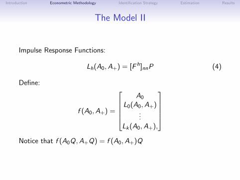
Impulse Response Functions:
Lh(A0,A+) = [F h]nnP (4)
Define:
f (A0,A+) =
A0
L0(A0,A+)...
Lk(A0,A+),
Notice that f (A0Q,A+Q) = f (A0,A+)Q

Introduction Econometric Methodology Identification Strategy Estimation Results
The Model III
• (A0,A+) and (A0Q,A+Q) are observationally equivalent
• sign and zero restrictions are satisfied if:
1. Zj f (A0,A+)Qej = 0
2. Sj f (A0,A+)Qej > 0
• How to choose the Q matrix?

Introduction Econometric Methodology Identification Strategy Estimation Results
Sign and Zero Restrictions: Intuition
• Recall the WOLD decomposition Theorem:
yt = B(L)PQQ′P−1ut
• we have to find an orthonormal matrix Q that satisfies thesign and zero restrictions
• construct a random matrix Q such that it satisfies the zerorestrictions
• check if the sign restrictions are also satisfied
• if yes keep the matrix Q and the structural parameters A0,A+
• if no, discard it and draw another Q

Introduction Econometric Methodology Identification Strategy Estimation Results
Constructing the matrix Q
Reformulate the Gram-Schmidt recursive algorithmDefine:
Rj(A0,A+) =
[Zj f (A0,A+)
Q′j−1
]where Qj−1 = [q1 . . . qj−1] and qj = Qej .
Theorem
1. Let j = 1.
2. Find a matrix Nj−1 whose columns form an orthonormal basisfor the null space of Rj(A0,A+).
3. draw xj from a standard normal distribution on Rn.
4. qj = Nj−1(N′j−1xj/ ‖ N
′j−1xj ‖).
5. If j = n stop; otherwise let j = j + 1 and move to step 2.

Introduction Econometric Methodology Identification Strategy Estimation Results
Algorithm for Sign and Zero Restrictions
1. Draw (B′+,Σ) from the posterior distribution of the reduced
form parameters.
2. Draw Q such that the structural parameters ((P−1)′Q,B
′+(P−1)
′Q)
satisfy the zero restrictions.
3. Keep the draw if Sj f (P−1)′,B′+(P−1)
′)qj > 0, where qj repre-
sents the j ′th column of Q.
4. Return to Step 1 until the required number of draws from theposterior distribution conditional on the sign and zero restric-tions has been obtained.

Introduction Econometric Methodology Identification Strategy Estimation Results
Baseline Identification I
We adopt the EE(1993) specification: (yt , y∗t , pt , nbrxt , rert , i
∗t , it)
Identification 1.
1. The federal funds rate is the monetary policy instrument andit reacts contemporaneously only to output and prices.The re-sponse coefficients of output and prices are non-negative.
2. For k periods the responses of prices and reserves are non-positive while the response of interest rates is non-negative.

Introduction Econometric Methodology Identification Strategy Estimation Results
Baseline Identification II
Label the first equation of the SVAR as the monetary policyequation:
yt′a0,1 = x
′tal ,1 + ε1t
⇔it = φyyt + φy∗y
∗t + φppt + φnbrxnbrxt + φrer rert + φi∗ i
∗t + a−1
0,71ε1t
Part 1 of our identification implies:
it = φyyt + φppt + a−10,71ε1t with φy > 0 and φp > 0.
For Part II we selected an horizont of 12 months

Introduction Econometric Methodology Identification Strategy Estimation Results
Baseline Identification II
Label the first equation of the SVAR as the monetary policyequation:
yt′a0,1 = x
′tal ,1 + ε1t
⇔
it = φyyt + φy∗y∗t + φppt + φnbrxnbrxt + φrer rert + φi∗ i
∗t + a−1
0,71ε1t
Part 1 of our identification implies:
it = φyyt + φppt + a−10,71ε1t with φy > 0 and φp > 0.
For Part II we selected an horizont of 12 months

Introduction Econometric Methodology Identification Strategy Estimation Results
Baseline Identification II
Label the first equation of the SVAR as the monetary policyequation:
yt′a0,1 = x
′tal ,1 + ε1t
⇔it = φyyt + φy∗y
∗t + φppt + φnbrxnbrxt + φrer rert + φi∗ i
∗t + a−1
0,71ε1t
Part 1 of our identification implies:
it = φyyt + φppt + a−10,71ε1t with φy > 0 and φp > 0.
For Part II we selected an horizont of 12 months

Introduction Econometric Methodology Identification Strategy Estimation Results
Baseline Identification II
Label the first equation of the SVAR as the monetary policyequation:
yt′a0,1 = x
′tal ,1 + ε1t
⇔it = φyyt + φy∗y
∗t + φppt + φnbrxnbrxt + φrer rert + φi∗ i
∗t + a−1
0,71ε1t
Part 1 of our identification implies:
it = φyyt + φppt + a−10,71ε1t with φy > 0 and φp > 0.
For Part II we selected an horizont of 12 months

Introduction Econometric Methodology Identification Strategy Estimation Results
Long-Run Multipliers
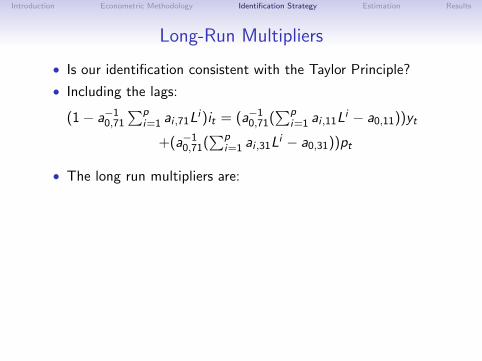
• Is our identification consistent with the Taylor Principle?
• Including the lags:
(1− a−10,71
∑pi=1 ai ,71L
i )it = (a−10,71(
∑pi=1 ai ,11L
i − a0,11))yt
+(a−10,71(
∑pi=1 ai ,31L
i − a0,31))pt
• The long run multipliers are:
Φy =∂i∗
∂y∗=
(a−10,71(
∑pi=1 ai ,11 − a0,11))
1− a−10,71(
∑pi=1 ai ,71)
(5)
Φp =∂i∗
∂p∗=
(a−10,71(
∑pi=1 ai ,31 − a0,31))
1− a−10,71(
∑pi=1 ai ,71)
(6)
Introduction Econometric Methodology Identification Strategy Estimation Results
Long-Run Multipliers
• Is our identification consistent with the Taylor Principle?
• Including the lags:
(1− a−10,71
∑pi=1 ai ,71L
i )it = (a−10,71(
∑pi=1 ai ,11L
i − a0,11))yt
+(a−10,71(
∑pi=1 ai ,31L
i − a0,31))pt
• The long run multipliers are:
Φy =∂i∗
∂y∗=
(a−10,71(
∑pi=1 ai ,11 − a0,11))
1− a−10,71(
∑pi=1 ai ,71)
(5)
Φp =∂i∗
∂p∗=
(a−10,71(
∑pi=1 ai ,31 − a0,31))
1− a−10,71(
∑pi=1 ai ,71)
(6)

Introduction Econometric Methodology Identification Strategy Estimation Results
Alternative Identifications
1. Scholl & Uhlig (2008): For 12 periods, the responses of pricesand reserves are non-positive while the response of interest ratesis non-negative.
2. Arias, Caldara, Rubio-Ramirez (2015): The federal fundsrate is the monetary policy instrument and it reacts contempo-raneously only to output and prices. The response coefficientsof output and prices are non-negative.

Introduction Econometric Methodology Identification Strategy Estimation Results
Estimation
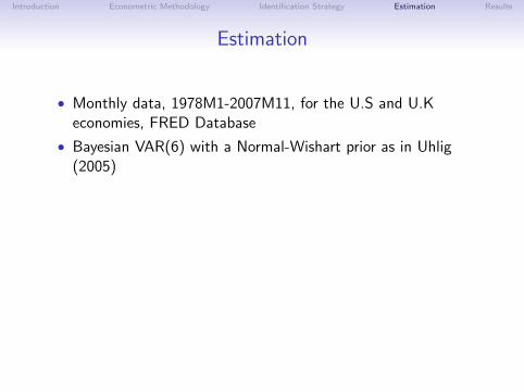
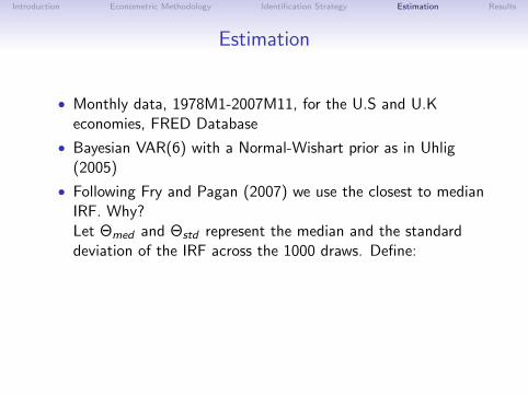
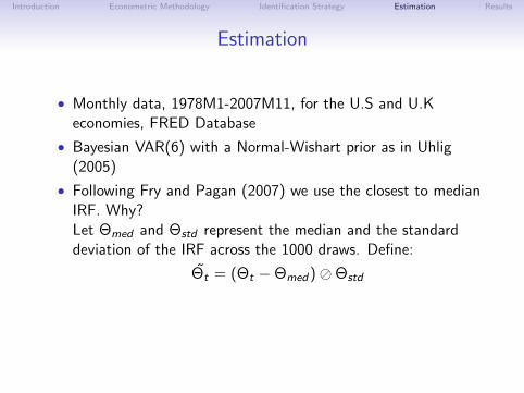
• Monthly data, 1978M1-2007M11, for the U.S and U.Keconomies, FRED Database
• Bayesian VAR(6) with a Normal-Wishart prior as in Uhlig(2005)
• Following Fry and Pagan (2007) we use the closest to medianIRF. Why?Let Θmed and Θstd represent the median and the standarddeviation of the IRF across the 1000 draws. Define:
Θt = (Θt −Θmed)�Θstd
Closest to Median IRF:
min vec(Θt)′vec(Θt)

Introduction Econometric Methodology Identification Strategy Estimation Results
Estimation
• Monthly data, 1978M1-2007M11, for the U.S and U.Keconomies, FRED Database
• Bayesian VAR(6) with a Normal-Wishart prior as in Uhlig(2005)
• Following Fry and Pagan (2007) we use the closest to medianIRF. Why?Let Θmed and Θstd represent the median and the standarddeviation of the IRF across the 1000 draws. Define:
Θt = (Θt −Θmed)�Θstd
Closest to Median IRF:
min vec(Θt)′vec(Θt)

Introduction Econometric Methodology Identification Strategy Estimation Results
Estimation
• Monthly data, 1978M1-2007M11, for the U.S and U.Keconomies, FRED Database
• Bayesian VAR(6) with a Normal-Wishart prior as in Uhlig(2005)
• Following Fry and Pagan (2007) we use the closest to medianIRF. Why?
Let Θmed and Θstd represent the median and the standarddeviation of the IRF across the 1000 draws. Define:
Θt = (Θt −Θmed)�Θstd
Closest to Median IRF:
min vec(Θt)′vec(Θt)
Introduction Econometric Methodology Identification Strategy Estimation Results
Estimation
• Monthly data, 1978M1-2007M11, for the U.S and U.Keconomies, FRED Database
• Bayesian VAR(6) with a Normal-Wishart prior as in Uhlig(2005)
• Following Fry and Pagan (2007) we use the closest to medianIRF. Why?Let Θmed and Θstd represent the median and the standarddeviation of the IRF across the 1000 draws. Define:
Θt = (Θt −Θmed)�Θstd
Closest to Median IRF:
min vec(Θt)′vec(Θt)

Introduction Econometric Methodology Identification Strategy Estimation Results
Monetary Policy Shocks under Scholl & Uhlig (2008)
10 20 30 40 50 60
0
0.1
0.2
0.3
0.4
Fed Funds
10 20 30 40 50 60
−0.25
−0.2
−0.15
−0.1
−0.05
0
0.05
U.K Output
10 20 30 40 50 60
−0.1
−0.08
−0.06
−0.04
−0.02
U.S CPI
10 20 30 40 50 60
−0.35
−0.3
−0.25
−0.2
−0.15
−0.1
−0.05
0Non−borrowed/Total reserves
10 20 30 40 50 60
−0.7
−0.6
−0.5
−0.4
−0.3
−0.2
−0.1
0
0.1
Real Exchange rate U.K/U.S
10 20 30 40 50 60−0.3
−0.2
−0.1
0
0.1
U.K interbank rate
10 20 30 40 50 60
−0.1
−0.05
0
0.05
0.1
0.15
U.S Output

Introduction Econometric Methodology Identification Strategy Estimation Results
IRFs from a Monetary Policy Shock under Arias etal.(2015)
10 20 30 40 50 60
−0.25
−0.2
−0.15
−0.1
−0.05
0
U.S Output
10 20 30 40 50 60
−0.04
−0.02
0
0.02
0.04
0.06
0.08
U.K Output
10 20 30 40 50 60−0.12
−0.1
−0.08
−0.06
−0.04
−0.02
0
U.S CPI
10 20 30 40 50 60
−0.2
−0.15
−0.1
−0.05
0
0.05
0.1
Non−borrowed/Total reserves
10 20 30 40 50 60−0.4
−0.3
−0.2
−0.1
0
0.1
Real Exchange rate U.K/U.S
10 20 30 40 50 60
−0.05
0
0.05
0.1
0.15U.K interbank rate
10 20 30 40 50 60
−0.2
−0.1
0
0.1
0.2
0.3
0.4
Fed Funds

Introduction Econometric Methodology Identification Strategy Estimation Results
FEVD of the MP Shock under Arias et al.(2015)
10 20 30 40 50 600
5
10
15
20
25U.S Output
10 20 30 40 50 600
0.5
1
1.5
2U.K Output
10 20 30 40 50 600
10
20
30
40
50U.S CPI
10 20 30 40 50 600
0.5
1
1.5
2
2.5Non−borrowed/Total reserves
10 20 30 40 50 600
0.5
1
1.5
2Real Exchange rate U.K/U.S
10 20 30 40 50 600
0.5
1
1.5
2
2.5
3
3.5U.K interbank rate
10 20 30 40 50 600
2
4
6
8
10
12
14Fed Funds

Introduction Econometric Methodology Identification Strategy Estimation Results
Long-run multipliers under Arias et al.(2015)
−16000−14000−12000−10000 −8000 −6000 −4000 −2000 0 2000 40000
1
2
3
4
5
6
7
8x 10
−4 Inflation Long−Run Multipliers: Φp
−4000 −3500 −3000 −2500 −2000 −1500 −1000 −500 0 500 10000
0.02
0.04
0.06
0.08
0.1
0.12
0.14
0.16
0.18
Output Long−Run Multipliers: Φy
.
i P(Φi > 0) P(Φi > 1) P(Φi > 20) P(Φi > 50) P(Φi > 100) P(Φi > 150) P(Φi > 200)
Φp 0.995 0.943 0.226 0.101 0.059 0.038 0.029
Φy 0.994 0.860 0.073 0.033 0.014 0.009 0.006

Introduction Econometric Methodology Identification Strategy Estimation Results
Is this plausible?
Scholl & Uhlig(2008) Identification:
• A contractionary monetary policy shock raises output inthe short-term (Is it expansionary?)
Arias et al.(2015) Identification:
• No significant effect of the identified monetary policy shockon the Federal Funds rate
• The shock explains only 13% on impact and 2% in thelong-run from the variations in Fed Funds
• 0.2% increase in interest rates causes output to fall by1-1.2%
• Probability of an inflation multiplier ≥ 50 or 100 is 10% and6% respectively
• Hard to justify the presence of an inflation multiplier of 100.

Introduction Econometric Methodology Identification Strategy Estimation Results
IRFs from a Monetary Policy shock under the BaselineIdentification
We restrict both the systematic component of monetary policy andthe IRFs
10 20 30 40 50 60
−0.15
−0.1
−0.05
0
0.05
U.S Output
10 20 30 40 50 60
−0.06
−0.04
−0.02
0
0.02
0.04
0.06
0.08
U.K Output
10 20 30 40 50 60
−0.12
−0.1
−0.08
−0.06
−0.04
−0.02
U.S CPI
10 20 30 40 50 60−0.25
−0.2
−0.15
−0.1
−0.05
0
Non−borrowed/Total reserves
10 20 30 40 50 60
−0.4
−0.3
−0.2
−0.1
0
Real Exchange rate U.K/U.S
10 20 30 40 50 60
−0.05
0
0.05
0.1
0.15
0.2
U.K interbank rate
10 20 30 40 50 60
0
0.1
0.2
0.3
0.4
0.5
Fed Funds

Introduction Econometric Methodology Identification Strategy Estimation Results
The MP Shock under the Baseline Identification
Jul78 Mar80 Nov81 Jul83 Mar85 Nov86 Jul88 Mar90 Nov91 Jul93 Mar95 Nov96 Jul98 Mar00 Nov01 Jul03 Mar05 Nov06
−2
−1.5
−1
−0.5
0
0.5
1

Introduction Econometric Methodology Identification Strategy Estimation Results
FEVD under the Baseline Identification
10 20 30 40 50 600
5
10
15
20U.S Output
10 20 30 40 50 600
0.5
1
1.5
2U.K Output
10 20 30 40 50 600
5
10
15
20
25
30U.S CPI
10 20 30 40 50 600
2
4
6
8Non−borrowed/Total reserves
10 20 30 40 50 600
2
4
6
8
10
12
14Real Exchange rate U.K/U.S
10 20 30 40 50 600
2
4
6
8
10U.K interbank rate
10 20 30 40 50 600
10
20
30
40
50
60Fed Funds

Introduction Econometric Methodology Identification Strategy Estimation Results
Long-run multipliers under Baseline Identification
0 5 10 15 20 25 30 35
0.02
0.04
0.06
0.08
0.1
0.12
Inflation Long−Run Multipliers: Φp
0 1 2 3 4 5
0.05
0.1
0.15
0.2
0.25
0.3
0.35
0.4
0.45
0.5
0.55
Output Long−Run Multipliers: Φy
i P(Φi > 0) P(Φi > 1) P(Φi > 5) P(Φi > 10) P(Φi > 20) P(Φi > 50)
Φp 1 0.9960 0.7650 0.2650 0.0390 0
Φy 1 0.5820 0 0 0 0

Introduction Econometric Methodology Identification Strategy Estimation Results
Conclusions
• We propose a new agnostic identification for open economySVARs...
• ...restricting both the systematic component of monetarypolicy and the IRFs
• this method yields more plausible results than the approches itbuilds on
• we find that an increase of 0.4-0.5% increase in interest ratescauses output to contract by 1.2% in the long-run
• exchange rate exhibits delayed overshooting